Leonardo Dias Pereira Minimizing Drill String Torsional ...
93
Leonardo Dias Pereira Minimizing Drill String Torsional Vibration Using Surface Active Control DISSERTA¸ C ˜ AO DE MESTRADO DEPARTAMENTO DE ENGENHARIA MEC ˆ ANICA Programa de P´os-gradua¸ c˜ ao em Engenharia Mecˆ anica Rio de Janeiro April de 2017
Transcript of Leonardo Dias Pereira Minimizing Drill String Torsional ...

Leonardo Dias Pereira
Minimizing Drill String TorsionalVibration Using Surface Active
Control
DISSERTACAO DE MESTRADO
DEPARTAMENTO DE ENGENHARIA MECANICA
Programa de Pos-graduacao em Engenharia
Mecanica
Rio de JaneiroApril de 2017
DBD
PUC-Rio - Certificação Digital Nº 1612778/CA

Leonardo Dias Pereira
Minimizing Drill String Torsional VibrationUsing Surface Active Control
Dissertacao de Mestrado
Dissertation presented to the Programa de Pos-Graduacao emEngenharia Mecanica of PUC-Rio in partial fulfillment of therequirements for the degree of Mestre em Engenharia Mecanica.
Advisor: Prof. Hans Ingo Weber
Rio de JaneiroApril de 2017
DBD
PUC-Rio - Certificação Digital Nº 1612778/CA

Leonardo Dias Pereira
Minimizing Drill String Torsional VibrationUsing Surface Active Control
Dissertation presented to the Programa de Pos-Graduacao emEngenharia Mecanica of PUC-Rio in partial fulfillment of therequirements for the degree of Mestre em Engenharia Mecanica.Approved by the undersigned Examination Committee.
Prof. Hans Ingo WeberAdvisor
Departamento de Engenharia Mecanica – PUC-Rio
Prof. Rubens Sampaio FilhoDepartamento de Engenharia Mecanica – PUC-Rio
Profa. Roberta de Queiroz LimaDepartamento de Engenharia Mecanica – PUC-Rio
Dr. Romulo R. AguiarSchlumberger Servicos de Petroleo – SLB
Prof. Marcio da Silveira CarvalhoVice Dean of Graduate Studies
Centro Tecnico Cientıfico – PUC-Rio
Rio de Janeiro, April 25th, 2017
DBD
PUC-Rio - Certificação Digital Nº 1612778/CA

All rights reserved.
Leonardo Dias PereiraThe author graduated in Mechanical Engineering at Univer-sidade Federal do Para (UFPA) at Belem, in 2011 and com-pleted a year of academic exchange in Mechanical and EnergyEngineering at the Istituit National Polytechnique de Grenoble(Grenoble INP - Ense3), France, in 2009. In 2013, he startedto work as Drilling and Completion Consultant at Hallibur-ton where he stayed for four years . There, he developed a re-markable experience working and communicating with multi-disciplinary and international/multi-cultural teams achievedby the Halliburton Advanced Fast Track Program in Houston,TX, in 2014. In 2015, he won the Strive for Excellence awardas the best Drilling and Completion project at Halliburton,using the relevant business acumen to implement WellheadMovement analysis for the Petrobras casing and tubing de-sign. In March 2016, the author started his master researchin the Laboratory of Dynamic and Vibration at the Depar-tamento de Engenharia Mecanica at PUC-Rio under the su-pervision of Hans Ingo Weber. The result of this research arepresented in this dissertation and focus on applying control ofstick-slip vibrations in drilling system.
Bibliographic dataPereira, Leonardo Dias
Minimizing Drill String Torsional Vibration Using SurfaceActive Control / Leonardo Dias Pereira ; advisor: Hans IngoWeber. – 2017.
v., 92 f.: il. ; 29.7 cm
Dissertacao (mestrado) – Pontifıcia Universidade Catolicado Rio de Janeiro, Departamento de Engenharia Mecanica.
par Inclui referencias bibliografias.
1. Engenharia Mecanica – Teses. 2. perfuracao depocos de petroleo. 3. controle de vibracao. 4. colunade perfuracao. 5. stick-slip. 6. vibracao torsional. I.Weber, Hans Ingo. II. Pontifıcia Universidade Catolica doRio de Janeiro. Departamento de Engenharia Mecanica. III.Tıtulo.
CDD: 621
DBD
PUC-Rio - Certificação Digital Nº 1612778/CA

To my parents, brothers and to my wife Jahnne Brandao for all the supportduring this period.
DBD
PUC-Rio - Certificação Digital Nº 1612778/CA

Acknowledgments
The author would like to acknowledge the Department of Mechanical Engi-
neering of PUC-Rio for the partnership that generating the support for this
research. Special acknowledgments to the Laboratory of Dynamics and Vi-
brations for permission to work and developed the study using its resources
and dependencies and specially to Wagner Epifanio for his strong support over
these years. The author would like to recognize Bruno Cayres, Fernanda Ohashi
and Abel Arieta for their contribution during the development of the technical
and conceptual part of this dissertation. Finally, the author also would like
to thank Prof. Hans Weber for his careful review of the manuscript and great
contribution and motivation to finalize this study.
DBD
PUC-Rio - Certificação Digital Nº 1612778/CA

Abstract
Pereira, Leonardo Dias; Weber, Hans Ingo (Advisor). Minimi-zing Drill String Torsional Vibration Using Surface Ac-tive Control . Rio de Janeiro, 2017. 92p. Dissertacao de Mestrado- Departamento de Engenharia Mecanica, Pontifıcia UniversidadeCatolica do Rio de Janeiro.
Part of the process of exploration and development of an oil field
consists of the drilling operations for oil and gas wells. Particularly for deep
water and ultra deep water wells, the operation requires the control of a very
flexible structure which is subjected to complex boundary conditions such as
the nonlinear interactions between drill bit and rock formation and between
the drill-string and borehole wall. Concerning this complexity the stick-slip
phenomenon is a major component, related to the torsional vibration and
it can excite both axial and lateral vibrations. That may cause premature
failure of drill-string components. So, the reduction and avoidance of stick-
slip oscillations are very valuable items in terms of savings and exploration
time. With these intentions, this study has the main goal of confronting
the torsional vibration problem using a real-time robust control strategy.
The approach is obtained following some steps such as: Open-loop analysis
of the drilling system considering a top-drive actuator and the drill-string
system; Design of a novel controller using different angular velocity setpoints
in a closed-loop system; Control of the torsional vibration considering the
nonlinearity due to friction interaction in the wall and in the donwhole
system; valuate a non-stop control system while drilling; Verification by
numerical simulations. In this presentation the theoretical basis behind the
drilling system will be given, as well examples of numerical results providing
a stable and satisfactory controlled drilling operation.
Keywordsoilwell drilling; vibration control; drill string ; stick-slip; torsi-
onal vibration.
DBD
PUC-Rio - Certificação Digital Nº 1612778/CA

Resumo
Pereira, Leonardo Dias; Weber, Hans Ingo. Minimizacao daVibracao Torcional em uma Coluna de Perfuracao Uti-lizando Controle com Acionamento na Superfıcie . Riode Janeiro, 2017. 92p. Dissertacao de Mestrado - Departamento deEngenharia Mecanica, Pontifıcia Universidade Catolica do Rio deJaneiro.
Parte do processo de exploracao e desenvolvimento de um campo de
petroleo consiste nas operacoes de perfuracao de pocos de petroleo e gas.
Particularmente para pocos de aguas profundas e ultra-profundas, a opera-
cao requer o controle de uma estrutura muito flexıvel que e sujeita a condi-
coes de contorno complexas, tais como as interacoes nao-lineares entre broca
e formacao rochosa ou entre a broca e a parede de poco. Quanto a esta com-
plexidade, o fenomeno stick-slip e um componente primordial relacionado a
vibracao torsional. Este pode excitar vibracoes tanto axiais quanto laterais.
Isso pode causar falha prematura de componentes de corda de perfuracao.
Assim, a reducao e eliminacao de oscilacoes do tipo stick-phase sao itens
muito valiosos em termos de economia financeira e de tempo de exploracao.
Com este proposito, este estudo tem como principal objetivo confrontar o
problema de vibracao torsional simulando uma estrategia de controle ro-
busto em tempo real. A abordagem e obtida seguindo alguns passos, tais
como: analise em malha aberta do sistema de perfuracao considerando um
atuador top drive e o sistema de coluna de perfuracao; concepcao de um
novo controlador que utiliza diferentes velocidades angulares de referencia
num sistema de controle de malha fechada; controle da vibracao torsional
considerando a nao-linearidade devida a interacao de atrito na parede do
poco e no fundo do poco; avaliar por meio de simulacoes sistemas de con-
trole ininterruptos durante a perfuracao; validacao dos modelos por meio
de simulacoes numericas. Esta dissertacao apresenta a base teorica por tras
do sistema de perfuracao, bem como exemplos de resultados numericos que
proporcionam uma operacao de perfuracao controlada estavel e satisfatoria.
Palavras–chaveperfuracao de pocos de petroleo; controle de vibracao; coluna de
perfuracao; stick-slip; vibracao torsional.
DBD
PUC-Rio - Certificação Digital Nº 1612778/CA

Table of contents
1 General introduction 181.1 Oilwell drilling overview 181.2 Motivation and objectives 231.3 Methodology 241.4 Outline of the dissertation 25
2 Literature review and preliminary concepts 272.1 Introduction 272.2 Literature review on active drill string control techniques 282.2.1 Classical control strategy 282.2.2 Robust control strategy 302.3 Preliminary concepts 332.3.1 Basic control definitions 332.3.1.1 Dynamical system 332.3.2 Open-loop and closed-loop systems 352.3.2.1 Open-loop system 352.3.2.2 Closed-loop system 362.3.3 Automatic control systems 382.3.4 Proportional, integral and derivative actions and controllers 392.3.4.1 Proportional action 392.3.4.2 Integral action 392.3.4.3 Derivative action 392.3.4.4 Proportional and integral controller (PI) 402.3.4.5 Proportional, integral and derivative controller (PID) 402.3.5 Model predictive control (MPC) 41
3 Mathematical modeling of the dynamical drilling system 453.1 Introduction 453.2 Dynamic modeling 453.2.1 Modeling approach: two degrees of freedom 453.2.1.1 Lower system: torsional pendulum 463.2.1.2 Upper system: DC motor 493.2.2 State-space equation of the electromechanical system 503.2.3 Friction torque modeling 50
4 Control design: open-loop and closed-loop approaches 534.1 Introduction 534.2 The open-loop analysis 534.2.1 Mathematical simplifications for the open-loop analysis 564.3 Closing the loop 574.3.1 Mathematical simplifications for the closed-loop control 584.4 Controlling nonlinear disturbance in drilling system 584.5 Stick-slip severity (SSS) 58
DBD
PUC-Rio - Certificação Digital Nº 1612778/CA

5 Analysis of the results 605.1 Introduction 605.2 Simulation results of the open-loop systems 605.3 Simulation results of the closed-loop system without disturbance 655.4 Simulation results of the closed-loop system with disturbance 675.4.1 Proportional and integral controller (PI) 675.4.2 Proportional, integral and derivative controller (PID) 725.4.3 Model predictive controller (MPC) 765.4.4 MPC and PID controllers (MPC+PID) 80
6 General conclusions and future works 836.1 Conclusions 836.2 Recommendations for future research 85
Bibliography 92
DBD
PUC-Rio - Certificação Digital Nº 1612778/CA

List of figures
1.1 Components of an oilwell drilling system. (Source: State of California,
2005) 201.2 Types of drill string vibrations. Source: Lopez, [1]. 211.3 Simulated Stick-Slip phenomenon. (Ω1− drill bit / Ω2− top drive). 22
2.1 Block diagram representing a general System. 332.2 Block diagrams of open-loop systems. 36
2.2(a)Open-loop system with feedforward control 362.2(b)Open-loop system without feedforward control 36
2.3 General block diagrams of a closed-loop system. 372.4 Major steps in model-based control design. (Adapted from Seborg
(2004) [2]). 422.5 Block diagram for MPC. (Adapted from Seborg (2004) [2]). 432.6 Basic concept for MPC. (Adapted from Seborg (2004) [2]). 44
3.1 Schematic of modern drilling system. 463.2 A drill string system modeled as a torsional pendulum. 473.3 Electrical equivalent circuit of armature. 493.4 Static + Coulomb + Negative damping friction model. 52
4.1 Block diagram of the closed-loop drilling system. 544.2 Process of opening the loop of the drilling system. 554.3 Block diagram of the open-loop DC motor. 554.4 Block diagram of the open-loop drill string. 554.5 Block diagram of the closed-loop drilling system without disturbance. 574.6 Stick-slip severity curves for the four control strategies. 59
5.1 The iterative open-loop flowchart used in the analysis. 615.2 Angular velocity and torque responses 63
5.2(a)(2kN ·m− 10kN ·m) 635.2(b)(12kN ·m− 20kN ·m) 635.2(c)(2kN ·m− 10kN ·m) 635.2(d)(12kN ·m− 20kN ·m) 63
5.3 Stick-slip severity curve for open-loop system without control. 655.3(a) 3D map 655.3(b) 2D map 65
5.4 Angular velocity responses for PID controller. 655.4(a) (2kN ·m− 10kN ·m) 655.4(b) (12kN ·m− 20kN ·m) 65
5.5 Calculated SSS and Bifurcation diagrams for PI controller. 685.5(a) 3D map 685.5(b) 2D map 685.5(c) Ωref = 79, 36 rpm 685.5(d) WOB = 160 kN 68
5.6 Closed-loop simulation of a top drive system (Case 1). 69
DBD
PUC-Rio - Certificação Digital Nº 1612778/CA

5.7 Closed-loop simulation of a top drive system (Case 2). 705.8 Closed-loop simulation of a top drive system (Case 3). 705.9 Closed-loop simulation of a top drive system (Case 4). 715.10 Closed-loop simulation of a top drive system (Case 5). 715.11 Calculated SSS and Bifurcation diagrams for PID controller. 72
5.11(a)3D map 725.11(b)2D map 725.11(c)Ωref = 79, 36 rpm 725.11(d)WOB = 160 kN 72
5.12 Nonlinear angular velocity responses for PID controller. 735.13 Nonlinear response of a PID Closed-loop system. 745.14 Calculated SSS and Bifurcation diagrams for MPC controller. 76
5.14(a)3D map 765.14(b)2D map 765.14(c)Ωref = 79, 36 rpm 765.14(d)WOB = 160 kN 76
5.15 Nonlinear angular velocity responses for MPC. 785.16 Nonlinear response of a MPC Closed-loop system. 785.17 80
5.17(a)3D map 805.17(b)2D map 805.17(c)Ωref = 79, 36 rpm 805.17(d)WOB = 100 kN 80
5.18 Nonlinear angular velocity responses for MPC+PID controller. 815.19 Nonlinear response of a MPC+PID Closed-loop system. 82
DBD
PUC-Rio - Certificação Digital Nº 1612778/CA

List of tables
3.1 Friction factors values used in the friction modeling. 52
5.1 Simulation parameters values. 625.2 Drill string and DC Motor open-loop results. 635.3 Attributes of the drill string step responses. 645.4 Attributes of the DC motor step responses. 645.5 PID controller parameters tuned. 655.6 Attributes of the drill string step responses. 665.7 Drill-string and Closed-loop simulation performance. 665.8 PI controller parameters tuned. 675.9 Cases of transition functions. 695.10 Attributes of the drill string step responses with PID. 745.11 Drill string with PID simulation performance. 755.12 Attributes of the drill string step responses with MPC. 775.13 Drill string with MPC simulation performance. 795.14 Attributes of the drill string step responses with MPC+PID. 815.15 Drill string with MPC + PID simulation performance. 82
DBD
PUC-Rio - Certificação Digital Nº 1612778/CA

Nomenclature
List of abbreviations
Peak first maximum value reached by y
ADS active damping system
BHA bottom hole assembly
D-OSKIL drilling oscillation killer
DC drill collars
DC motor direct current motor
DOF degrees of freedom
DRPM downhole RPM
DTF data transmission frequencies
DWOB downhole WOB
FEM finite element methods
GA genetic algorithms
GUI graphical user interface
HWDP heavy weight drill pipe
KSEPL Koninklijke/Shell Exploratie en Produktie Laboratoruim
MPC model predictive controller
N/A Not Applied
NMPC nonlinear model predictive controller
OPEC Organization of the Petroleum Exporting Countries
OSKIL oscillation killer
PI proportional and integral controller
PID proportional, integral and derivative controller
ROP rate of penetration
RPM rotations per minute
SRPM surface RPM
SSS stick-slip severity
STOR surface torque
DBD
PUC-Rio - Certificação Digital Nº 1612778/CA

STRS soft torque rotary system
TFC torque feedback control
TOB torque on bit
WOB weight on bit
List of symbols
%OS Overshoot – percentage overshoot (relative to yfinal)
y(kt) predicted outputs
µ constant friction coefficient
ν Poisson ratio
Ωmax1 maximum angular velocity of the drill bit
Ωmin1 minimum angular velocity of the drill bit
Ω1 angular velocities measured at the downhole (DRPM)
Ω2 angular velocities measured at the surface (SRPM)
Ωdyn final speed of the sticking regime
Ωref reference angular velocity
ρbha BHA mass density
ρdp drill string mass density
τp Peak time – time at which this peak is reached
τr Rise time – time to first reach the steady-state value
τs Settling time – time to reach and remain above the steady-statevalue
ϕ1 angular displacements of the BHA
ϕ2 angular displacements of the top drive
C1 equivalent viscous damping coefficient of downhole
C2 equivalent viscous damping coefficients of surface
Dr damping factor of the mud
E Young’s modulus
e control error (e = [r(t)− ym(t)])
E(t) control error (E(t) = [Ωref − Ω2])
ec stability error criterion
DBD
PUC-Rio - Certificação Digital Nº 1612778/CA

I armature current
Ibha area moment of inertia for the BHA
Idp area moment of inertia for the drill pipe
IDbha BHA inner diameter
IDdp drill string inner diameter
J1 equivalent mass moment of inertia of the BHA
J2 equivalent mass moment of inertia of the surface
k equivalent torsional stiffness coefficient of the drill pipe
kt actual sampling instant
kd derivative gain, (kd = kpTd)
ke electromotive force constant
ki integral gain, (ki = kp
Ti)
kp proportional gain
kt motor torque constant
L electrical inductance
Lbha BHA length
Ldp drill string length
ODbha BHA outer diameter
ODdp drill string outer diameter
Pf−c Coulomb factor
Pf−nd negative damping approximation
Pf−neg “negative” friction factor when the angular velocity reaches nega-tive values
Pf−s static factor
Pf (Ω1) velocity-dependent proportional friction factor
R electrical resistance
r manipulated variable
Sinput input signal of the controller
SSS stick-slip severity - instability criterion
Tm torque input signal of the drilling system
DBD
PUC-Rio - Certificação Digital Nº 1612778/CA

T1 nonlinear function representing the downhole TOB
Td derivative time constant
Ti integral time constant
Tol speed tolerance
u(kt) actual input
uc control signal
Um voltage input signal of the actuator / motor input voltage
Vemf back-electromotive force (back-emf)
Vinput voltage input signal of the actuator
y output angular velocity of the drill string
ym controlled variable
A1 set parameters coefficient matrix
A2 input parameter vector
A3 output parameter matrix
C matrix of damping
J matrix of inertia
K matrix of stiffness
q′ first derivative of the state vector
T torque disturbance vector
y output vector
u scalar control law
q state vector
DBD
PUC-Rio - Certificação Digital Nº 1612778/CA

Excellence is an art won by training and habit-uation. We do not act rightly because we havevirtue or excellence, but rather we have thosebecause we have acted rightly. We are what werepeatedly do. Excellence, then, is not an actbut a habit.
Aristotle, The Story of Philosophy.
DBD
PUC-Rio - Certificação Digital Nº 1612778/CA

1General introduction
1.1Oilwell drilling overview
Over the last 20 years, the world has watched the volatility on global
supply/demand mechanism and on the oil and gas market expectations.
Demand for oil is related to economic activity, so the higher the economic
activity the higher oil demand. As to the seasonal aspects, it spikes for example
during winter time in the northern hemisphere. On the other hand, supply is
determined by weather (can affect production) and by geopolitical issues (can
affect the crude oil price) [3].
For example, in the mid-2000s, global demand for crude oil was rising.
This situation resulted in a tight market and steep price increases [4]. However,
global oil prices have fallen sharply over the past two years, resulting in one of
the most dramatic declines in the price of oil in recent history. The oil prices
have collapsed from around $114 in June 2014 to $28 in February 2016 [3].
To be more specific, between December 2010 and July 2014, oil barrel
prices were quoted, on average, above 100 dollars [3]. Then, still in 2014, the
Organization of the Petroleum Exporting Countries (OPEC) - responsible for
supplying 40% of the world’s crude oil - increased its oil production by the
largest volume in almost three years. Meanwhile, the US continued to increase
its shale production. As a result, the global production increased faster than
its demand, creating a long market [4].
To make the shale oil exploration economically viable, the United States
has invested in several resources, such as an advanced oil exploration and
production infrastructure. The unconventional technologies used for shale
extraction could be used to boost the production of existing conventional oil
fields globally [3].
The use of increasingly sophisticated drilling techniques and huge im-
provements in cost efficiencies has not only reduced the costs associated with
the production of shale oil, but it has also made the extraction resemble a
manufacturing process. In other words, the quantity produced can be altered
in response to price changes with relatively ease. This is not the case for conven-
DBD
PUC-Rio - Certificação Digital Nº 1612778/CA

Chapter 1. General introduction 19
tional oil extraction which requires large capital expenditure and lead times.
The drilling time for shale oil continues to become increasingly more ef-
ficient. Two years ago, it took six weeks to drill a single well. Today, it takes
approximately two weeks. Cost-saving technologies include more efficient ex-
ploration methods, onsite automation systems, and intelligent production mon-
itoring software. Beyond cheaper hardware, the next saving opportunity lies
in advances including more automation: intelligent control systems requiring
less physical workforce, less downtime and improving yields of existing wells.
It is worth mentioning that due to the current advances in shale oil production
it now takes only 20 days and $10 million to drill for shale while it takes $10
billion and five to ten years to launch a deep water oil project [3].
The example of shale recovery history demonstrates that the actual
organizational model of oil and gas industry is no longer sustainable with
oil prices below $50 a barrel. Christopher et al. (2016) [5] describes what
they call the “potentially game-changing disruptions that may lead oil and
gas companies to rethink their operating models fundamentally”. Here, two of
the main reasons are pointed to elucidate what this study intends to emphasize:
1. “A world of resource abundance is leading to sustained lower oil prices
and a focus on cost, efficiency, and speed. Talent is no longer scarce,
exploration capability is less of a differentiator, mega-projects are not
the only way to grow and market opportunities may only be economical
for the earliest movers in a basin. Meanwhile, conventional, deep water,
unconventional, and renewable assets each require a distinct operating
model that cannot be delivered optimally from a single corporate center”.
2. “Profound technological advances are disrupting old ways of working and
enabling steep changes in productivity. Jobs, including knowledge work,
are being replaced by automation on a large scale, and those that remain
require increased human-machine interaction. Data generation continues
to grow exponentially, as every physical piece of equipment wants to
connect with the cloud. This explosion of data - combined with advanced
analytic and machine learning to harness it -creates opportunities to
fundamentally re-imagine how and where work gets done”.
Then, to address these challenges, this study focuses its efforts on the
conventional drilling operations. These are an important part of a process
of exploration and development of oilfields. In this context, the rotary drilling
system is considered the most used drilling technique in the petroleum industry.
This process involves rock failure by a rotating drill bit. To rotate this drill
bit from the top-end position (surface), the drilling rig’s power source is used
DBD
PUC-Rio - Certificação Digital Nº 1612778/CA

Chapter 1. General introduction 20
to turn a rotary table. A mechanism, composed of the master bushing and
kelly, is used to transmit the rotation from the rotary table to the drill string.
An electric or hydraulic top drive unit is used as an alternative to
the conventional arrangement on modern rigs. In this situation, the rotational
energy is transmitted directly from the rig’s power source to the drill string.
The subsurface component through which torque is transmitted from the
surface to the bottom of the drilling system (downhole) is the drill string. The
drill string consists of connected lengths of drill pipes, the bottom hole
assembly (BHA), and the drill bit. The BHA is the portion of the drill
string between the drill pipe and the drill bit. It is made up, primarily, of drill
collars (DC) and heavy weight drill pipe (HWDP). These components,
shown in the Fig.1.1, are responsible for the open hole creation.
Figure 1.1: Components of an oilwell drilling system. (Source: State of California,
2005)
The operational sequences to drill a hole section are based on standard
drilling procedures. Of course, they may change over the years. But they are
always monitored by a driller who can adjust critical drilling parameters from
a control device in the rig floor. For example, the driller may set up the top
DBD
PUC-Rio - Certificação Digital Nº 1612778/CA

Chapter 1. General introduction 21
drive to rotate at a constant revolution (rotations per minute - RPM).
Also, the driller may adjust the amount of hook load applied [that reflects
on the weight on bit (WOB)]. Other parameters, such as torque on bit
(TOB) and the rate of penetration (ROP), also allow the driller to be
informed of any potential problem [6, 7, 8].
Particularly for deep water and ultra-deep water wells, the operation
described above requires the control of a very flexible structure (the drill string
length may be up to 5 km for ultra deep water whereas its diameter is typically
less than 150 mm) which is subjected to complex boundary conditions. The
complexity may be due to the nonlinearity between drill bit and rock formation
and between the drill string and borehole wall. Hence, dynamic drilling systems
can present complex vibrational states and there is a strong need to understand
them in order to better control the drilling operation and improve the ROP.
Previous studies have identified three types of vibrations that may occur
during drilling operations, as illustrated in Fig. 1.2. They are classified as
[9, 10]:
Torsional - large amplitude fluctuations of the angular velocity due to
large torsional flexibility of the drilling assembly.
Axial - motion of drilling components along its own longitudinal axis.
Lateral - whirl motion due to the out-of-balance of the drill string.
Figure 1.2: Types of drill string vibrations. Source: Lopez, [1].
According to some authors [10, 11] the stick-slip behavior of the drill
string represents one of the most severe case (in terms of oscillation amplitudes
DBD
PUC-Rio - Certificação Digital Nº 1612778/CA

Chapter 1. General introduction 22
and drill string life cycle reduction) of torsional vibration and instability on
the drilling system dynamics. More specifically, the torque applied at the bit is
governed by the bit-rock interaction law [12, 13] and depends on the angular
velocity at the rock-bit interface. Basically, the nonlinearity in the relationship
between the pair WOB, RPM defines the behavior of the system: the stick-
slip is observed at low RPM or high WOB; and it does not observed at high
RPM and low WOB [13].
In recent years, several controlled systems were designed to maintain an
angular velocity nearly a constant value at the surface. But this situation does
not assure the same condition at the drill bit. That happens because the stick-
slip phenomenon may drive the system to a highly oscillating angular velocity
at the bottom. In extreme cases, this oscillation may lead to a complete arrest of
the drill bit (stick phase), while the drill string is still being torqued-up. Then,
the drill bit rotation is released (slip phase) and it rotates at a much higher
angular velocity than the desired (up to 5 times the adjusted velocity). Fig. 1.3
illustrates the stick-slip behavior when theWOB = 120 kN and Ωref = 60 rpm.
350 400 4500
50
100
150
200
250
RPM
Time [s]
Ω1
Ω2
Figure 1.3: Simulated Stick-Slip phenomenon. (Ω1− drill bit / Ω2− top drive).
The stick-slip can be defined as a periodic and stable oscillation of the
angular velocity for several drilling conditions [14]. This oscillation uses the
energy accumulated to self-excite itself and, generally, disappears as the desired
RPM is increased and/or the WOB is reduced under certain drilling conditions.
However, at higher angular velocities, some other complex phenomena appear,
such as lateral vibrations (backward and forward whirling), impacts of drill
string on borehole wall, and parametric instabilities.
DBD
PUC-Rio - Certificação Digital Nº 1612778/CA

Chapter 1. General introduction 23
Therefore, to improve the drilling conditions for relatively low angular
velocities, several studies on drill string dynamics, with focus on dynamical
models and control design, exist in the literature. Some of them will be
presented in section 2.2.
1.2Motivation and objectives
Drilling operation represents an expensive phase of the oil and gas
prospecting. They represent approximately 40% of all exploration and pro-
duction (E&P) costs [15]. Due to its high costs, drilling has become the main
challenge of oil and gas exploration. The drill string vibration is responsible for
a large percentage of failures due to different excitations sources, such as non-
linear bit-rock interactions, mass imbalance, misalignment, mud motor, and
friction between the drill pipe and borehole wall.
Studies focusing on torsional vibrations of drill chords have shown that
stick-slip behavior occurs 50% of the time in drilling processes and can
excite both axial and lateral vibrations. These vibrations can cause premature
equipment failure [16]. Thus, it is clear that the reduction and avoidance of
torsional vibrations (stick phase) are very valuable in terms of savings and
operating time.
Since the vibration problems were detected and identified in the drilling
process, several approaches have been suggested, both in industry and litera-
ture, to model and control these vibrations. Some of the approaches were driven
to the surface system. Most of them dealt with the torsional behavior and the
suppression of the stick-phase in the stick-slip oscillations [17]. Moreover, the
nonlinearity and the system parameter incertitude have been modeled into the
control design process.
Another important consideration to be taken in the system is the time
delay in measurements. They might cause problems while running real-time
controls [18].
The scope of this study is to minimize the torsional vibration problem
of the drill bit using existing control strategies. In addition, evaluation and
confronting their performances will be considered. The specific objectives deal
with:
– Open-loop analysis of the drilling system considering a saturated and a
non-saturated top drive actuator.
– Application of existing control strategies using different torque/velocity
input in a closed-loop system.
DBD
PUC-Rio - Certificação Digital Nº 1612778/CA

Chapter 1. General introduction 24
– Control of the torsional vibration considering the nonlinearity due to
friction interaction with the wall and in the donwhole system.
– Evaluate a non-stop control system while drilling.
– Improvement on a developed experimental reduced setup to future veri-
fication and validation of the models.
1.3Methodology
The methodology required to evaluate the performance of the control
drilling system are based on five steps:
1. The modeling of the mechanical and mathematical representation of the
drilling system is developed.
2. An open-loop analysis is performed to a simplified model using a linear
motor and a two degrees-of-freedom (DOF) system. In this system a
friction model with parameters that generate torsional vibrations at the
bit is proposed, i.e. a settled relation involving WOB, surface torque
(STOR), TOB, and desired input RPM (Ωref ).
3. The state-space environment is designed to reconstruct the states vari-
ables needed to control the bit vibration.
4. The closed-loop analysis starts assuming a set of parameters for different
controllers.
5. Two situations are analyzed concerning the control strategies:
(a) Only surface parameters such as STOR, surface RPM (SRPM), and
WOB are known.
(b) The surface and the downhole measurements (such as TOB, downhole
RPM [DRPM], and downhole WOB [DWOB]) are known.
Another concern is the way to collect the measurements from the surface
or from the downhole to be sent to a control device. In fact, there are
many different data transmission frequencies (DTF) for both cases. The DTF
can be estimated from the type of transmission used in field, i.e. telemetry
signals or wired drill pipe [19]. Thus, for both surface and downhole cases, a
determination must be made as to whether or not it is possible to control the
drilling system for a specific number of DTFs (chosen according to the existing
DFTs).
Finally, the methodology elaborated here can be continuously used
for systems with varying number of DOFs, chosen according to increasing
modeling complexity of the drill string components.
DBD
PUC-Rio - Certificação Digital Nº 1612778/CA

Chapter 1. General introduction 25
One of the most important results of this study is a program performed
in Simulink environment to achieve the explained methodology. The Simulink
software was used because it provides a graphical user interface (GUI) for
building models as block diagrams. Hence, the interface can build models,
simulate and analyze the dynamical drilling system. Then, the proposed model
simulations assume the drill string as a torsional pendulum composed of a
generic number of DOF. In addition, the user can set the number of DOF.
For result analysis of the proposed drilling system, in Simulink environ-
ment, it can plot chosen inputs and outputs parameters. So, it is possible to
predict the dynamic behavior of the model in surface and downhole.
Another important achievement of this study is that it uses the Simulink
to compare different control strategies used to optimize drilling performance.
This comparison aims to determine the most effective control strategy among a
variety of alternatives. For this propose an optimization criterion and a robust
stability criterion of the system are combined using the Simulink toolbox.
Initially, there are four control strategies used in this comparison:
– Proportional and Integral Controller (PI)
– Proportional, Integral and Derivative Controller (PID)
– Model Predictive Controller (MPC)
– Proportional, Integral and Derivative and Model Predictive Controller
(PID + MPC).
In the end, the study will discuss about an experimental test rig con-
structed in the laboratory for future validation and a test of a reduced real-
time model. This system will be further discussed in the section of suggestions
for future studies.
1.4Outline of the dissertation
The dissertation is based on work performed in the Pontifical Catholic
University of Rio de Janeiro (PUC- Rio) for a scientific and technological
graduate program to obtain the Master degree. The dissertation is organized
as following. First, in Chapter 1 the general introduction about the oil and
gas industry and the proposed problem are presented. To understand what
was done in the past the Chapter 2 presented a literature review in control
torsional vibration and ends the Chapter with the preliminary concepts of
the control strategies used in this study. Then, Chapter 3 presented the
Mathematical modeling to describe the problem and further simplifications of
the proposed model. Chapter 4 presented the methodology used to desing the
control strategies adopted. The simulation results and a preliminary analisis
DBD
PUC-Rio - Certificação Digital Nº 1612778/CA

Chapter 1. General introduction 26
are presented in Chapter 5. Finally, the study conclusions and future works
are discussed in Chapter 6.
DBD
PUC-Rio - Certificação Digital Nº 1612778/CA

2Literature review and preliminary concepts
2.1Introduction
The overview about the oilwell industry presented in the last chapter
showed that stick-slip vibration is one of the primary causes of drill string
component failures. For that reason, several studies and actions have been
taken to optimize the drilling operation and/or avoid drill string vibration.
Nevertheless, there is still a giant field to be developed about this concern that
also motivated the current study.
Over the past 70 years, there were hundred of references about the
vibration on drilling systems. Many of them were taken to develop analysis
methodologies, evaluation technologies and control methods for the drill string
vibrations. Moreover, according to the control theory and control engineering
knowledge, these control methods can be divided into passive control, active
control, and semi-active control [20]. However, only in the last 30 years a
significant variety of control actions have been developed to suppress the stick-
slip phenomenon. There are so many options that it is impossible to determine
which approach is the best, as they all have benefits for some drilling conditions
[21].
In this chapter, approaches for stick-slip vibration suppression are focused
on, and the developments in the theoretical background are conducted. First,
the approaches for stick-slip vibration active control are reviewed by grouping
the literature references under two different categories: classical and robust
control strategies. Then, the theoretical basis of control, applied to drilling
systems, is briefly reviewed. Furthermore, additional reviews about drill string
vibration can be found on the references [21, 20].
DBD
PUC-Rio - Certificação Digital Nº 1612778/CA

Chapter 2. Literature review and preliminary concepts 28
2.2Literature review on active drill string control techniques
2.2.1Classical control strategy
Halsey et al. [16] were the very first to model an active control strategy
to eliminate, or at least reduce, self-excited torsional drill string vibrations
occuring due to the stick-slip phenomena. The Torque Feedback Control (TFC)
developed by Halsey et al. had the goal to correct the demanded speed
according to the torque signal measured at the rotary table. They verified
their results by field experimentation on a full-scale research drilling rig and
used accelerometers in the downhole components. They concluded that the
conventional speed controller made the top drive very insensitive to torque load
variations. They also concluded that such a control system leads to smoother
rotation of the bit which can lead to a reduction in axial and lateral vibrations
of the drill string.
In 1992, Sananikone et al. [8] proposed to make a comparison between
the TFC, the combined motor current and acceleration feedback system, and
the motor current only feedback system. Drilling field operations had been
done to evaluate the performance looking at the ”reflection”. This coefficient is
related to the vibration wave. This energy is reflected back down in the drill
string. Some applications which should be added on were addressed in this
study, such as a surface torque limiting system to prevent excessive winding
up of the drill pipe. They concluded that the TFC described has the advantage
of being simpler to install than the simple torque feedback system, reducing
drill string vibrations by 90% and of not requiring ”re-tuning” for different drill
string lengths.
Still in 1992, a modified version of the TFC was developed and field-
tested by Koninklijke/Shell Exploratie en Produktie Laboratoruim (KSEPL)
and Deutag Drilling Inc. of Germany [22, 23]. This system was called Soft
Torque Rotary System (STRS) and relied on a minor modification of the
electronic speed control system on the drive system. If the current of the
rotary drive motor was a measure of the torque at the surface, the current
could be directly used to control the velocity of the motor, thus eliminating
the need for torque measurement at the rig floor [22, 23]. The principles of
the STRS are detailed by Worrall et al. [24] patent. Javanmardi and Gaspard
[23] also commented on the successful field test performed in several top drive
rigs, but they focused primarily on the Mobile Bay application.They observed
that different sizes of drill strings exhibit different vibratory characteristics,
DBD
PUC-Rio - Certificação Digital Nº 1612778/CA

Chapter 2. Literature review and preliminary concepts 29
so the STRS has to be tuned for each drill pipe size used on the rig. They
concluded that the STRS had significantly reduced torque fluctuations (up to
80%), torsional drill string vibrations, and the bit stick-slip motions.
Jansen & van den Steen [25] also explored the idea of the TFC based
on the same principles explained in [16, 8]. In this study Jansen applied an
active damping system (ADS) describing how it strongly reduced a threshold
value of the angular velocity by using feedback control. They highlighted
the nonlinear relation between torque and angular velocity at the bit. This
relation generates the self-excited torsional drilling vibrations. They also used
the electrical variables to perform the ADS such as Sananikone [8] did, but
without the accelerometer at the motor shaft. However, the main contribution
of this article is the ease use of the TFC and the ADS. Jansen concluded the
paper discussing the applicability of such system for different types of motors,
other than DC motors. This application is shown in their other study, reference
[26].
The linear H∞ control design technique proposed by Serrarens [7] aimed
to suppress the stick-slip oscillations and transient behavior of the angular
velocity improved over a PD control system. Serrarens was the first to apply
a robust closed-loop system to treat the nonlinear friction influence. This
paper concluded that the designed controller is sufficiently robust against
variations in the drill string length. The paper also compared the time
domain results of the H∞ to the first-order control system STRS. It brought
significant improvements to the drilling performance because the H∞ controller
suppresses limit cycles for backlash torques which are much higher than those
handled by the STRS controller. These results were proven experimentally and
the numerical simulations showed great resemblance with the experimental
responses.
Kriesels et al. [15] discussed the use of some specific combined technology
and methodology developed to solve drill string torsional vibration and its
effects when using STRS. The control system developed by van den Steen
[6] operated as a small modification of the electric motor and it suppressed
torsional oscillations of the drill string. The article showed how other types of
vibrations could be prevented by using vibration analysis software. It proved
that applying these methods the ROP would increase and equipment damages
would also decrease.
In 1999, Tucker et al. [27] modeled the torsional vibration of a vertical
drill string driven by a controlled torque at the surface top drive and subjected
to torsional friction at the bit. Tucker approached the problem of the volatility
with a classical controller as PI. They explored alternative mechanisms to
DBD
PUC-Rio - Certificação Digital Nº 1612778/CA

Chapter 2. Literature review and preliminary concepts 30
disable the need for repeated retuning as the drilling characteristic varies. The
paper studied the behavior of two continuous models based on axisymmetric
configuration and a simplified forced torsional pendulum. In both cases the
superiority of the proposed torsional rectification method over conventional
control techniques had been demonstrated. Finally, the authors believed that
a more robust controller (in terms of instability) could be constructed by
combining existing speed controllers with torsional rectification control. That
is because the combination of controllers would act on different concerns about
drilling process, such as non-linear controllers and speed linear controllers.
2.2.2Robust control strategy
To compensate the nonlinear friction effect, Abdulgalil & Siguerdidjane
[14] proposed a friction compensation method using in a simple nonlinear
controller for a drill string system. Therefore, the application of a nonlinear
friction model, reported in the reference [14], allowed the authors to study
and suggest a compensation technique for stick-slip combined with the PI
controller. To confirm the proposed method efficiency some simulations were
performed, demonstrating the relevance of the nonlinear friction compensation
method.
In 2005, Abdulgalil & Siguerdidjane [28] proposed another robust strat-
egy based on a nonlinear control design approach called Backstepping control.
The backstepping technique represented a powerful and systematic strategy
that recursively interlaces the choice of a Lyapunov function with the feedback
control design. Afterwards, Abdulgalil & Siguerdidjane [9] presented another
robust PID controller based on sliding surface function. This function worked
in conjunction with an input-state control design capable to deal with a non-
linear drilling system due to uncertainties in the measured signals. The sliding
mode technique is applied by choosing the bit angular velocity error as the
sliding surface. Considering that, Abdulgalil & Siguerdidjane papers may be
considered pioneers in this application even if Serrarens [7] methodology is
used.
A different methodology to eliminate undesired limit cycles in nonlinear
systems was proposed by Canudas-de-Wit et al. [29] in 2005. They named
the Oscillation Killer (OSKIL). This strategy was applied to suppress stick-
slip oscillations in the well drill string system by using the WOB as an
additional control variable to extinguish limit cycles when they occur. They
also created a new strategy: the Drilling Oscillation Killer (D-OSKIL) [30].
The D-OSKIL mechanism permitted elimination of the stick-slip in the drilling
DBD
PUC-Rio - Certificação Digital Nº 1612778/CA

Chapter 2. Literature review and preliminary concepts 31
system without changing the imposed angular velocity. This angular velocity
is fixed by a typical speed controller.
Then, in 2006, Corchero et al. proposed a stability analysis of a variant
of the D-OSKIL mechanism. This analysis has shown that this algorithm is
globally asymptotically stable [31], thus, effectively eliminating the stick-slip
oscillations. Canudas-de-Wit wrote two other papers describing this mechanism
in [32, 33]. The D-OSKIL was also applied by Jijon et al. in 2010. They
combined the control system with an unknown parameter adaptive observer
that measured the angular velocity of the bit. The observer was implemented
in a testbed using a mud-pulse telemetry and an acoustic data transmission
over a drill string.
In 2007, Navaro-Lopes and Cortes proposed to use a nonlinear approach
to reduce and/or avoid the torsional stick-slip phenomenon. The sliding mode
control is the nonlinear approach applied to the multi-DOF drilling system
used to eliminate the bit sticking phenomena [34]. The drilling system consists
of four kinds of elements divided in the top-rotary system, the drill pipes, the
drill collars, and the bit. In their article Navaro-Lopes and Cortes also showed
robustness under parameters variations [34].
In 2009, Karkoub et al. proposed to use PID and lead-leg controllers
combined with genetic algorithms (GA) to control the drilling system. The
reason that made this technique attractive to control systems was its capability
to perform with minimal knowledge of the plant under investigation [35].
The problem is converted to an optimization problem while it selects the
optimum controller parameters. The authors simulated the open-loop dynamics
compared to the closed-loop one. Finally, the controllers were designed using
different objective functions and parameter search limits, concluding that the
results were satisfactory [35].
In 2010, the slide mode control was also applied by Qi-zhi et al. to
a conventional model describing the torsional behavior of a generic vertical
oilwell drill string. In this article the main task was to design a controller that
would drive the bit velocity to the reference as fast as possible and maintain it
without any stick-slip oscillations [36]. They applied three reaching laws in the
sliding mode in the drilling process. Then, the simulation results showed that
the control laws were capable of controlling the bit speed, had faster dynamic
responses and suppressed stick-slip in oil well drill string [36]. After that, Qi-zhi
et al. used the idea of introducing another surface discontinuity and forcing
the system to evolve along this surface [37]. In this study the sliding-mode
control was applied as described in their first article ([36]). They focused the
analysis on a problem of linear time-variant system stability with time-delay.
DBD
PUC-Rio - Certificação Digital Nº 1612778/CA

Chapter 2. Literature review and preliminary concepts 32
Furthermore, some specific relationships between the former observer’s gain
and the delayed term was found with respect to the time delay through the
Lyapunov’s method.
Fubin et al. presented in 2010 the adaptive PID control strategy of the
drilling system to eliminate the stick-slip phenomenon on the bit. The system
is composed of two parts: the linearization method input controller and the
adaptive PID controller [38]. The adaptive controller was designed to reduce
or eliminate the problem caused by the fixed control parameters. Otherwise,
when internal characteristics and external disturbances change in large scale,
the system performance usually falls substantially [38]. Furthermore, the
simulation results showed that this controller had good control characteristics
and fast dynamic response. It could eliminate stick-slip oscillation of the drill
bit and improve the performance of rotary table [38].
The model-based control approach also was largely used as a robust con-
trol strategy to control the drill string vibrations. Puebla and Alvarez-Ramirez
(2008) [39] were one of the first to design a model-based controller. Basically,
they used two control configuration to guarantee the system robustness: the
called cascade control scheme and decentralized control scheme, both applied
to numerical simulations. In their study they considered a 2-DOF system and
several bit-rock interaction models in four different case studies.
Johanessen and Myrvold (2010) [40] seem to be the first to use the MPC
(a model-based controller) to control the stick-slip behavior. They used the
Nonlinear MPC (NMPC) approach to address the problem in a numerical
drilling system. Also, they compared this strategy to the SoftSpeed device
to prove the robustness of the developed system. Breyholtz (2012) [41] also
cited the MPC as a good alternative to control the pressure during drilling
operations. He advocates for its use in other applications. This study was based
on the Modes of Automation, defined as the different levels of automation
strategy using human-machine interactions.
Vromen (2015) [42] affirmed that the existing industrial controllers were
deficient to control systems under the increasingly challenge operational con-
dition. Then, he described two main reasons for this deficiency. First, the in-
fluence of multiple dynamical modes of the drill string for torsional vibrations.
Next, the uncertainty in the bit-rock interaction. Therefore, to eliminate the
vibrational effects in the drilling system controllers were designed and experi-
mentally validated. The dynamic model adopted a bit-rock interaction model,
with severe velocity-weakening effect, and the controller design were based on
a lumped-parameter model, exhibiting the most dominant torsional flexibil-
ity modes and based on a finite-element method representation of a realis-
DBD
PUC-Rio - Certificação Digital Nº 1612778/CA

Chapter 2. Literature review and preliminary concepts 33
tic drilling system with a multi-modal model of the torsional dynamics. Two
controller design methodologies that meet these requirements have been de-
veloped. The first is based on nonlinear observer-based controller synthesis
approach for Lur’e-type systems with discontinuities. The second controller
design strategy is based on the robust H∞-control. Moreover, these active con-
trollers had been applied to an experimental setup designed and realized by
the author. Also, he applied passive down-hole tools for stick-slip suppression.
2.3Preliminary concepts
In this section some basic drilling associated terminologies will be pre-
sented. This terminology and methodology can be used on any other control
strategies. Also, it presents introductory concepts of control systems as they
are applied on further investigation. These control strategies are those that
best fitted the subject of this study. Moreover, brief illustrations on graphical
block diagrams are presented related to each control law.
2.3.1Basic control definitions
2.3.1.1Dynamical system
Several references has minutely described the full control theory for differ-
ent applications and control strategies, such as [43, 44, 45, 46, 2]. Nevertheless,
general elements of control are discussed and presented in this section, such as
the elements of a general system, illustrated in Fig. 2.1.
Process
DisturbanceVariable
ManipulatedVariable
ControlledVariable
Figure 2.1: Block diagram representing a general System.
A system can be, generally, defined as a combination of elements and de-
vices that act together to perform a certain objective. Although the possibility
of applying this concept to many different dynamical phenomena, even ab-
stracts such as those encountered in economics, the current study investigates
the behavior of a dynamical mechanical system: the drilling system.
DBD
PUC-Rio - Certificação Digital Nº 1612778/CA

Chapter 2. Literature review and preliminary concepts 34
The corresponding dynamical system may be described with the physical
elements of the drilling system illustrated in Fig. 1.1. This physical system will
have its behaviors adequately described by mathematical models in Chapter
3.
In this study it is very important to notice that the actual drilling system
is composed of controller plus actuator plus drill string, what strongly differs
from the majority of several other studies.
For simplification, the full dynamical drilling system may be divided in
two subsystems: DC motor subsystem and the drill string subsystem. Both
systems together form a multivariable system that will be presented next.
Moreover, both subsystems can be illustrated in a block diagram as two
separated plants, defined by Ogata [46] as pieces of equipment or only sets of
machine parts functioning together with the purpose of performing a particular
operation.
Nowadays, the main objective of those subsystems/plants is still to
perform the drilling process by means of the driller control action. Even
considering all the innovation developed over the years. However, the driller
has only control over three parameters at surface [47]: the hook-load (generates
WOB); the surface rotary speed (SRPM); and the flow rate. These parameters
are known as manipulated variables, also called control variables.
The driller also observes other three output parameters: the downward
speed of the kelly (top end of the drill string when submitted to rotary table
torque); the motor current of the rotary table or top drive; and the standpipe
pressure. These parameters are the controlled variables that stand for the
quantity or condition that is measured and controlled, usually maintained at
some desired value referred to as setpoint or reference value. Moreover, for
each controlled variable, there is an associated manipulated variable adjusted
by the controller to keep the controlled variable value at or near their setpoint
value.
To finalize the general system discussion, the disturbance variable is
defined as the parameter that tends to drive the controlled variable away from
the desired, reference or setpoint conditions. The disturbance can be internal
(generated within the system) or external (generated outside the system). In
the current case study, the main disturbance variable is the TOB, generated
by the friction interaction between the drill bit and rock surface.
DBD
PUC-Rio - Certificação Digital Nº 1612778/CA

Chapter 2. Literature review and preliminary concepts 35
2.3.2Open-loop and closed-loop systems
There are several distinctions between working with an open-loop drilling
system and working with a closed-loop drilling system. Therefore, in order
to elucidate these differences and other important aspects of the two system
approaches, this section will discuss the details of each.
2.3.2.1Open-loop system
First, the open-loop system and analysis are presented. Despite the
simplicity of this application, it has not received the relevance it deserves over
the last years. Only a few studies in the literature have realized the powerful
tool that this analysis strategy can provide when used to understand behaviors
of an unknown system. When talking about studies on drilling systems the
number of studies is even smaller.
The open-loop system is especially beneficial to users because it provides
more sensitivity and experience about the system being study, so, as conse-
quence, they can develop increasingly robust control systems.
This strategy has notable features, such as the output signal without
influence or effect on the controlled variable. Therefore, the open-loop system
is known as a non-feedback system. This means that once the control strategy
is set up, the output is neither measured nor fed back to compare with the
input signal.
The current drilling process can be a good practical example of open-loop
and manual control system when the driller does not take action on the system
after it is in operation.
The elements of an open-loop system with and without control are
represented in the block diagrams shown in Figs. 2.2.
Generally, there are two open-loop system models: controlled or not
controlled. In other words, for an open-loop analysis in a drilling system, the
process may be equipped with a controller plus an actuator (Fig. 2.2(a)) or
just with an actuator driven by an input signal 2.2(b). For the purpose of this
study, the open-loop system is considered without the controller.
The Sinput is the input signal of the controller in the block diagram of
Fig. 2.2(a). The Vinput and uc are the voltage input signal of the actuator, the
u is the torque input signal of the drilling system. The y is the output angular
velocity of the drill string.
It is evident that if the drilling system is affected by the TOB or any
other disturbance, there is a need for control. Therefore, to prevent errors
DBD
PUC-Rio - Certificação Digital Nº 1612778/CA

Chapter 2. Literature review and preliminary concepts 36
Controller Actuator Systemuc uSinput y
2.2(a): Open-loop system with feedforward control
Actuator SystemuVinput y
2.2(b): Open-loop system without feedforward control
Figure 2.2: Block diagrams of open-loop systems.
from occurring due to disturbances, a control action (manual or automatic)
should be applied. However, the open-loop analysis, to be performed in this
study, will not have any type of disturbance because one of the objectives
of this investigation is to understand the behavior of each dynamical system
without any disturbance.
In summary, the main characteristics of an Open-loop System are defined
as being [48]:
– There is no comparison between actual and reference values.
– An open-loop system has no self-regulation or control action over the
output value.
– Each input setting determines a fixed operating position for the controller.
– Changes or disturbances in external conditions do not result in a direct
output change1.
2.3.2.2Closed-loop system
The drilling process totally depends on the driller to inspect the, previ-
ously defined, controlled variables visually. As a result, he manages the manip-
ulated variables [hook-load (WOB), SRPM, and flow rate] to adjust the process
to achieve the setpoint value of the controlled variable. Therefore, when the
driller takes action, he is manually closing the loop of the system.
The closed-loop system can use the same components presented in
the open-loop system with controller (Fig. 2.2(a)). But the difference is the
addition of one or more feedback loops. These loops may utilize actual angular
velocity signal measurements and compare them with the desired angular
velocity value (setpoint). These measures are called feedback signals and may
be collected by a sensor or a transducer.
The difference between the setpoint and the actual angular velocity (by
mean of feedback signal) generates an error signal. Then, this signal is treated
1Unless the controller setting is altered manually
DBD
PUC-Rio - Certificação Digital Nº 1612778/CA

Chapter 2. Literature review and preliminary concepts 37
by the controller to obtain a control signal, also called the manipulated variable.
Finally, the manipulated variable can be used to stabilize a disturbed dynamic
system.
For this study the closed-loop analysis of the drilling process will be
performed with disturbance and without disturbance. Furthermore, the closed-
loop control system, also known as feedback control system, is represented by
the block diagram shown in Fig. 2.3.
The Ωref is the reference signal of the system to be compared to the
measured angular velocity ym in the block diagram of Fig. 2.3 and generates
the error signal E(t). The Um is the voltage input signal of the actuator, the Tm
is the torque input signal of the drilling system. The y is the output angular
velocity of the drill string.
Controller DC Motor System
Disturbance (T1)
Um Tn
Measurements
Ωref E(t) y
−
ym
Figure 2.3: General block diagrams of a closed-loop system.
The feedback control systems are the most used control methodology of
the industry. A quick literature review on stick-slip vibration control shows
that the most part of the studies about the topic uses the feedback theory for
analysis and design[20, 21, 49]. It is the simplest way to automate the control
process by generating a control action dependent of the comparison between
the output measured signal and the desired signal.
In summary, the main characteristics of Closed-loop Control are defined
as being [50]:
– To reduce errors by automatically adjusting the systems input.
– To improve stability of a disturbed system.
– To increase or reduce the system sensitivity.
– To enhance robustness against external disturbances to the process.
– To produce a reliable and repeatable performance.
DBD
PUC-Rio - Certificação Digital Nº 1612778/CA

Chapter 2. Literature review and preliminary concepts 38
2.3.3Automatic control systems
The previous sections discussed about the manner in which the automatic
and manual controller produce the control signal using the feedback or feedfor-
ward control systems. Now, the control strategies used in the current study are
discussed in more details. Well known industrial closed-loop controllers were
chosen according to their control actions, such as:
– Proportional and integral controller (PI)
– Proportional, integral and derivative controller (PID)
– Model predictive control (MPC)
The cited controllers can be categorized according to general approaches
related to control system design. Thus, this study focus on two of them [2]:
1. Conventional approach. The classical control strategies, such the PID-
types, have been largely applied in oilwell industry using the feedback or
feedforward laws. Therefore, the control system design can be developed
based on this approach in a linear and nonlinear system. Moreover, once
the control system is installed in the plant the controller tuning strategy
can start to be applied.
2. Model-based approach. The model-based approach uses the dynamical
model to predict the behavior of the drilling system by means of a
mathematical model of the process (also called internal model). The
suggested mathematical model has three possible applications: (i) it can
be used as the basis for model-based controller design methods; (ii) it can
be incorporated directly in the control law; (iii) the model can be used
in a computer simulation to evaluate alternative control strategies and to
determine preliminary values of the control settings [2].
Clearly, both approaches have strong industrial application. However,
control strategies under the conventional approach are the most used in
industrial processes. For example, Astrom (1994) [43] determined that more
than 95% of the control loops were of PID type and most of this loops used PI
control. In his turn, Breyholtz (2012) [41] determined that the PID controllers
are by far the most widely used control technology in the oilwell industry.
On the other hand, if a conventional control system can not be satis-
factory, an alternative approach, such as the model-based control, may be
applied. In that case, this study intends to use the MPC as a sophisticated
enough strategy to control the complex dynamical drilling system.
According to what Breyholtz (2012)[41] determined in his study: it is not
necessary completely replacing human resources in the rig floor by autonomous
DBD
PUC-Rio - Certificação Digital Nº 1612778/CA

Chapter 2. Literature review and preliminary concepts 39
systems. However, the automation must improve performance during normal
drilling operations while allowing the driller to intervene in varying degrees in
case of abnormal events.
2.3.4Proportional, integral and derivative actions and controllers
To apply any control action in the closed-loop drilling system, the
Controller box (see Fig. 2.3) can be replaced by a well defined classical strategy
such as P, PI, PD, PID controller (or a combination of them). Each P,I and
D actions and two control strategies (PI and PID) will be presented in this
section to adjust the angular velocity parameter.
Even when referring to stick-slip active control, the PID controller is
said to be the ”bread and butter” of control engineering. Hence, this simple
controller has become a test bench for many new ideas in control and it has
proved its utility with a satisfactory performance when compared with other
developed strategies.
2.3.4.1Proportional action
The Proportional feedback controller is defined as the control signal
made to be linearly proportional to the error signal for small errors. Thus,
the proportional controller can be seen as an amplifier that adjust the gain up
to the desired velocity. However, this controller may cause a static or steady
state error in response to a constant velocity setpoint and may not be capable,
by itself, to eliminate the disturbance completely.
2.3.4.2Integral action
The integral action is the one responsible for improving the steady state
accuracy (by eliminating the error) of a control system under the proportional
action. So, it makes sure that the controlled variable agrees with the velocity
setpoint in steady state. However, at the end of the process the integral action
can cause a worse transient response.
2.3.4.3Derivative action
The derivative action is an important tool to improve the closed-loop
stability. On this action of control the magnitude of the controller signal is
proportional to the rate of range of the actuating error signal. Besides its
DBD
PUC-Rio - Certificação Digital Nº 1612778/CA

Chapter 2. Literature review and preliminary concepts 40
anticipatory characteristics, this action can never anticipate an action that
has not yet taken place.
2.3.4.4Proportional and integral controller (PI)
The principle used in the SoftTorque control system (PI controller) is
based on the proportional and integral control theory. The same used in the
current study. However, the only difference is the use of the DC motor dynamic
on the full scale system modeled here. The PI control strategy is also known as
the standard velocity controller and it is applied to correct the error between
the actual and desired angular velocity of the top drive actuator (rotating
motor) on the drilling system.
So, based on the PI actions described in this section and on the general
block diagram of Fig. 2.3, the mathematical control law has the form:
uc(t) = kp [r(t)− ym(t)] + ki
∫ t
0[r(t)− ym(t)]dt
= kp e(t) + ki
∫ t
0e(t)dt (2-1)
where uc is the control signal, ym is the controlled variable, r is the manipulated
variable and e is the control error (e = [r(t) − ym(t)]). kp is the proportional
gain. ki is the integral gain and can be represented as ki = kp
Ti. Ti is the integral
time constant.
2.3.4.5Proportional, integral and derivative controller (PID)
Several applications of PID control has been applied to the dynamical
drilling system, as seen in the references [38, 36, 41, 51]. But few of them
have used the controller plus actuator in their dynamical system, as is used
in the current study. As discussed before, the PID control has three terms
with specific characteristics that combined provides the classical PID control
strategy. Some of the advantages and disadvantages are:
(P) - Proportional:
Advantage - It reduces error response to disturbance and increase
the speed of response.
Disadvantage - It has a much larger transient overshot [45].
(I) - Integral:
Advantage - It can eliminate the steady-state error.
DBD
PUC-Rio - Certificação Digital Nº 1612778/CA

Chapter 2. Literature review and preliminary concepts 41
Disadvantage - It costs the deterioration in the dynamic response.
(D) - Derivative:
Advantage - It damps the dynamic response and improves the
closed-loop stability.
Disadvantage - It is late in correcting for an error.
In summary, the most used control method provides feedback, eliminates
steady-state error through integral action, and anticipates the future through
derivative action [43].
The mathematical representation of the PID controller is based on the
proportional, integral and derivative actions, described in previous sections,
which has the form:
uc(t) = kp [r(t)− ym(t)] + ki
∫ t
0[r(t)− ym(t)]dt+ kd
d
dt[r(t)− ym(t)]
= kp e(t) + ki
∫ t
0e(t)dt+ kd
d
dte(t) (2-2)
where uc is the control signal, ym is the controlled variable, r is the manipulated
variable and e is the control error (e = [r(t) − ym(t)]). kp is the proportional
gain, ki is the integral gain and kd is the derivative gain. ki = kp
Ti, kd = kpTd.
The Ti is the integral time constant and the Td is derivative time constant.
2.3.5Model predictive control (MPC)
Among the various model-based control laws previously presented (see
section 2.2) this study focuses on the MPC as the strategy to deal with complex
dynamic drilling systems. The strategy works when a reasonable accurate
drilling dynamic model is available. Hence, the MPC design was chosen due to
two main characteristics: it deals naturally with multivariable control problems
and allows the system to operate closer to its constraints [2].
Fig. 2.4 exposes the flowchart with the major steps to design and install
a control system using the model-based approach [2].
The MPC system is illustrated in the block diagram in Fig. 2.5. It
is a feedback control law that uses the outputs of a well-defined dynamic
Model and the current measurements of the drilling Process to predict the
future values of the output variables, such as angular velocity. The comparison
between the actual (Process outputs) and Model outputs generates the feedback
signal called Residuals to feed the Prediction block. The Prediction block uses
an optimization algorithm to predict these variables. This optimization is
DBD
PUC-Rio - Certificação Digital Nº 1612778/CA

Chapter 2. Literature review and preliminary concepts 42
Formulatecontrol
objetives
Information fromexisting operation
(if available)
Managementobjectives
Developprocess model
Computersimulation
Field data(if available)
Physical andmathematical
principles
Devise controlstrategy
Process con-trol theory
Experience withexisting operation
(if available)
Computersimulation
Select controlhardware
and software
Vendor In-formation
Install controlsystem
Adjust con-troller settings
FINAL CON-TROL SYSTEM
= Engineering activity = Information base
Figure 2.4: Major steps in model-based control design. (Adapted from Seborg
(2004) [2]).
performed at each time step with the same horizon and uses the updated
measures/estimates of states and the disturbances. Predicted output values
feed the Setpoint calculations and Control calculation. These boxes generate
the Input variables. Also, system constraints, such as upper and lower limits,
DBD
PUC-Rio - Certificação Digital Nº 1612778/CA

Chapter 2. Literature review and preliminary concepts 43
can be considered at each time step during performance [2, 40].
PredictionControl
Calculation
Set-pointCalculation
Process
Model
PredictedOutputs
Set-point(targets)
ModelOutputs −
ProcessOutputs
Inputs
Residuals
Figure 2.5: Block diagram for MPC. (Adapted from Seborg (2004) [2]).
The MPC system application provides benefits, such as:
– Prevent violations of input and output constraints.
– Directs the output variables to their optimal setpoints while maintaining
other outputs within specified ranges.
– Prevents excessive movement of input variables.
– Controls as many variables as possible when a sensor or actuator is
unavailable.
The control calculations are based on current measurements and pre-
dictions of the future values of the outputs. The predictions are made using,
typically, a linear dynamic model. But for very nonlinear processes, it can be
advantageous to predict future outputs values using a nonlinear dynamic model
[2].
The purpose of the MPC control calculations is to determine a sequence of
control movements to move the predicted response to the setpoint optimally.
An illustration of what occurs when a MPC is applied can be seen in Fig.
2.6. At the moment of current sampling, denoted by kt, the MPC strategy
calculates a set of M values of the input u(kt + i − 1), i = 1, 2, ...,M. The
set consists of the current input u(kt) and M − 1 future inputs. The inputs
are held constant after the M control moves. The inputs are computed so that
the set of P predicted outputs y(kt + i), i = 1, 2, ..., P reaches the setpoint
optimally. The number of predictions P is referred to as prediction horizon
while the number of control moves M is called control horizon [2].
DBD
PUC-Rio - Certificação Digital Nº 1612778/CA

Chapter 2. Literature review and preliminary concepts 44
k − 1 k k + 1 k + 2 k +M − 1 k + P
FuturePastNow
Prediction Horizon, P
Control Horizon, M
Setpoint (target)
Future control action
Past control action
Predicted future output
Past output
Figure 2.6: Basic concept for MPC. (Adapted from Seborg (2004) [2]).
DBD
PUC-Rio - Certificação Digital Nº 1612778/CA

3Mathematical modeling of the dynamical drilling system
3.1Introduction
One of the key role in the model-based control design is the development
of a dynamic model of the drilling process, as mentioned in Fig. 2.4. The
theoretical model is developed based on physical and mathematical principles
to simulate the dynamic torsional system in order to provide insights into
system behavior. This dynamic is based on a simplified drilling system model
(only 2-DOF), considering some assumptions and including operational model
parameters of a realistic full-scale system.
This chapter is concerned with the development of the torsional dynamic
model of the drilling system. For that propose, first, the dynamic modeling and
the corresponding equation of motion are derived. In this step, the influence
of some drilling components, such as top drive unit, drill pipes, BHA and drill
bit, on the system behavior will be considered. Then, the state-space equation
of the electromechanical system is presented as a combination of the torsional
drill string and DC motor dynamic models. Finally, the friction model used to
generate the stick-slip is presented.
3.2Dynamic modeling
3.2.1Modeling approach: two degrees of freedom
The rotary system is the most used method for drilling wells in the oil
and gas industry. In the last few years, the oil industry process development
promoted the top drive unit to the top of the list of the preferred drive systems
used in the drilling operations. A simple schematic of the full scale drilling
system is illustrated in Fig. 3.1.
To simplify the model analysis some considerations will be assumed, e.g.,
the borehole is a vertical trajectory. Also, the lateral and axial motions of the
drill bit will not be considered. Thus, the current study deals only with torsional
vibrations modes of the drill string. Although the various ways to represent the
DBD
PUC-Rio - Certificação Digital Nº 1612778/CA

Chapter 3. Mathematical modeling of the dynamical drilling system 46
top drive
drill pipe
drill bitBHA
Figure 3.1: Schematic of modern drilling system.
dynamic of the drill string (e.g., i - one-mode [12]; ii - beam model with the
finite element method (FEM) [13]; iii - discrete system with one, two or more
DOF [34, 52]) it was chosen for this study a discrete 2-DOF system because
of its intuitive ease to be implemented in a numerical simulation.
The torsional drilling process will be divided in two dynamic subsystems:
the upper system and the lower system. The first part (upper), acting as a
flywheel, is driven by a DC motor, represented by the top drive unit that
delivers torque on the surface. The upper dynamic has a considerable impact
on the full dynamical behavior. On the other hand, the lower part consists of
drill pipes, BHA and a drill bit. Both subsystems are physically connected to
perform the drilling operation. Therefore, both dynamics will be investigated
here.
3.2.1.1Lower system: torsional pendulum
Although the importance given to the upper system modeling in this
study (see section 3.2.1.2), the main physical behavior occurs in the lower
system. For example, the stick-slip phenomenon disturbs measurements done
DBD
PUC-Rio - Certificação Digital Nº 1612778/CA

Chapter 3. Mathematical modeling of the dynamical drilling system 47
by components of the lower system while drilling. Therefore, the torsional
vibration control has a crucial role for the accuracy of the modeling of this
system.
Furthermore, it can be noticed from the literature about stick-slip vibra-
tions that a great part of the studies only consider the lower system in their
dynamical modeling. Those characteristics make this dynamical system the
most relevant part to approach the torsional vibration problem.
Fig. 3.2 illustrates the drill string dynamical model. It assumes that
the lower system behaves as a torsional pendulum when drilling. So, the
torsional drilling dynamics can be modeled as a two DOF system, for simplicity.
Moreover, constant WOB and a reference angular velocity (Ωref ) are imposed
on the surface inertia (J2). The model can be considered very simple in
comparison to the different models presented in literature and since the 2-
DOF represents only few specific realistic situations, but it is an important
step for the purpose of this study.
C1
C2
J1
J2
k
Ω1,ϕ1
Ω2,ϕ2
Tm
T1
Figure 3.2: A drill string system modeled as a torsional pendulum.
The two DOF model was also used by Cayres (2013) [52] in his study.
Thus, the model consists of two damped inertia mechanically coupled by an
elastic drill string where the surface torque (STOR) Tm is imposed by a motor
at the top end, as shown in Fig. 3.2. The drill string is homogenous along its
entire length and considered as a single linear torsional spring with stiffness
coefficient k [38, 36]. The main variables observed for this analysis are the
DBD
PUC-Rio - Certificação Digital Nº 1612778/CA

Chapter 3. Mathematical modeling of the dynamical drilling system 48
Surface RPM (SRPM) Ω2 and the Downhole RPM (DRPM) Ω1 measured on
the top drive and on the BHA, respectively.
The corresponding equations of motion of the drill string system are
represented by the model of torsional dynamics in Eq. 3-1. J1 00 J2
Ω1
Ω2
+
C1 00 C2
Ω1
Ω2
+
k −k−k k
ϕ1
ϕ2
=
−T1
Tm
(3-1)
where ϕ1 and ϕ2 are the angular displacements of the BHA and the top drive,
Ω1 and Ω2 are the angular velocities measured at the downhole and surface
positions. J1 and J2 are the equivalent mass moment of inertia of the BHA
and of the upper system (a combination of the drill pipes and the surface
component such as drive motor, gear box and top drive). C1 and C2 are the
equivalent viscous damping coefficients, k is the equivalent torsional stiffness
of the drill pipe, and T1 is the nonlinear function representing the downhole
torque on bit (TOB).
J1 = ρbha Ibha Lbha (3-2)
J2 = ρdp Idp Ldp (3-3)
where Ldp and Lbha are the lengths of the components. ρbha and ρdp are the
mass densities. Idp and Ibha are the area moments of inertia for the drill pipe
and the BHA, respectively. They can be written as:
Ibha = π
32(OD4bha − ID4
bha) (3-4)
Idp = π
32(OD4dp − ID4
dp) (3-5)
where ODbha and ODdp are the outer diameters. IDbha and IDdp are the inner
diameters.
The equivalent viscous damping coefficients (C1, C2) are written in terms
of the damping factor of the mud Dr,
C1 = DrLbha (3-6)
C1 = DrLdp (3-7)
The torsional stiffness of the drill pipe is:
k = GIdpLdp
(3-8)
DBD
PUC-Rio - Certificação Digital Nº 1612778/CA

Chapter 3. Mathematical modeling of the dynamical drilling system 49
where G is the shear modulus G = E
2(1 + ν) . E is the Young’s modulus and ν
is the Poisson ratio.
For this simple two DOF modeling, the matrix of inertia J, damping
C, and stiffness K from Eq. 3-1 are illustrated as follows:
J =J1 0
0 J2
, C =C1 0
0 C2
, K = k −k−k k
3.2.1.2Upper system: DC motor
The main difference between the model presented in Cayres [52] (and
several other studies) and the model studied here is the implementation of the
electrical equations of the top drive motor, first presented by Jansen et al. [25].
The electric circuit of the armature and the free-body diagram of the rotor are
shown in Fig. 3.3. The behavior of the DC electronic motor has its dynamical
principles represented by two linear models: (1) The mechanical equation of
free-body diagram of the rotor. (2) The electric circuit equation of armature.
Um
RI
L
Vemf
Ω2, Tm
Figure 3.3: Electrical equivalent circuit of armature.
The equation of motion of the rotor has already been presented in Eq.3-
1, but it is modified based on the Kirchhof’s law and Newton’s Second law.
Therefore, it is assumed that the magnetic field is constant and the torque is
directly proportional to the armature current I. By this time, the armature
current is the electric variable of DC motor and the angular velocity is the
mechanical variable as presented in the reduced linear equations below.
L I +RI + Vemf = Um (3-9)
Vemf = ke Ω2 (3-10)
Tm = kt I (3-11)
DBD
PUC-Rio - Certificação Digital Nº 1612778/CA

Chapter 3. Mathematical modeling of the dynamical drilling system 50
where I is defined as armature current. R and L are electrical resistance
and electrical inductance, respectively. Um is the motor input voltage. Vemf
represents the back-electromotive force (back-emf) related to the angular
velocity Ω2. ke and kt parameters are respectively the electromotive force
constant and the motor torque constant.
3.2.2State-space equation of the electromechanical system
By substituting the motor torque and the back-emf (3-10) in the Eqs. 3-1
and 3-9 and rearranging both together, the state-space equation of electrome-
chanical system can be expressed as:
q′ = A1q + A2u+ T (3-12)
y = A3q (3-13)
where q is the state vector, A1 is the set parameters coefficient matrix,
A2 the input parameter vector controlled by the scalar control law u, T is
the torque disturbance vector, A3 is the output parameter matrix, and y is
the output vector.
Thus, the state-variables are written in matrix form as:
q =
ϕ1
ϕ2
Ω1
Ω2
I
, A1 =
0 0 1 0 00 0 0 1 0
−J−1K −J−1C00
0 0 0 −ke/L −R/L
, T =
00
−T1/J1
Tm/J2
0
,
y =
y1
y2
y3
y4
y5
, A2 =
0000
1/L
, A3 =
0 0 0 0 00 0 0 0 00 0 1 0 00 0 0 1 00 0 0 0 0
As the initial conditions of the dynamic system will be considered
only the torsional behavior, the surface and downhole angular velocities and
displacements are zero.
3.2.3Friction torque modeling
The nonlinear resistive torque at the bit properly modeled based on a
cutting process model because of the characteristic of the bit-rock interaction.
DBD
PUC-Rio - Certificação Digital Nº 1612778/CA

Chapter 3. Mathematical modeling of the dynamical drilling system 51
But for simplicity it can be modeled for a friction law T1 depends on the
WOB, the friction coefficient µ and the friction factor Pf (Ω1) (dependent
on the velocity). The function covers static (Pf−s) + Coulomb (Pf−c) +
approximation of negative damping (Pf−nd) regions. The composite function
tries to simulate the friction model based on the nonlinear bit-rock interaction.
In the literature, it is easy to find references of the friction models, such
as cited by Germay et al. [53] and with different degrees of complexity such as
Karnop and LuGre models [54, 55]. Based on that, the most common friction
models are presented below, including:
(a) Velocity weakening laws [56],
(b) Stiction plus Coulomb friction [7, 26],
(c) Stribeck effect1
The corresponding friction law can cause torsional vibrations in the drill
string system. To better emulate this behavior in the model the relation is
assumed to be practical, nonlinear, and suitable for dynamic analysis and
controller synthesis. The practicality of the model is observed when:
– It reproduces the required phenomenon (stick-slip);
– The model presented is as simple as possible and fast to implement on
numerical analysis.
For this reason, the Eq. 3-14 describes how the resistive torque at the
drill bit is modeled based on the following friction law.
T1 = µ ·WOB · Pf (Ω1) (3-14)
where µ is a constant friction coefficient, WOB is the weight on bit, also
constant in the model, and Pf (Ω1) is the velocity-dependent proportional
friction factor.
The set-valued proportional friction factor law is modeled as a compo-
sition of others literature models and has been suited to generate stick-slip
behavior under specific conditions.
Pf (Ω1) =
Pf−s, for Ω1 < Tol
Pf−nd, for Tol ≤ Ω1 < Ωdyn
Pf−c, for Ω1 ≥ Ωdyn
Pf−neg, for Ω1 < 0
(3-15)
1Characterized by a decreasing friction-velocity map localized around zero velocity.
DBD
PUC-Rio - Certificação Digital Nº 1612778/CA

Chapter 3. Mathematical modeling of the dynamical drilling system 52
where Pf−s, Pf−c are described in table 3.1. The negative damping approxima-
tion is described by the general relation Pf−nd = αΩ1 + β (being α = −0.076and β = 1.3). Tol is a stipulated speed tolerance (Tol = 0.01) and Ωdyn is the
final speed of the sticking regime (Ωdyn = 8.5 rad/s) . Pf−neg is a “negative”
friction factor when the angular velocity reaches negative values.
The complete set-valued friction model is shown in Fig. 3.4 and the
coefficients considered, as presented in Eq. 3-15, are defined in Tab. 3.1.
Factor Description Value Setpoints [rad/s]Pf−s Static factor 1.30 0.01Pf−c Coulomb factor 0.65 8.50Pf−neg ”Negative” factor -0.20 ≤ 0
Table 3.1: Friction factors values used in the friction modeling.
−15 −10 −5 0 5 10 15−0.5
0
0.5
1
1.5
rad/s
Pf(
Ω1)
Friction Factor
Static factor Dynamic factor
"Negative" factor
Figure 3.4: Static + Coulomb + Negative damping friction model.
DBD
PUC-Rio - Certificação Digital Nº 1612778/CA

4Control design: open-loop and closed-loop approaches
4.1Introduction
This chapter presents the open-loop and closed-loop systems for a set of
input parameters, analyzing the application of some different types of control
laws used to control the drill string torsional vibration. Thus, the focus of these
control strategies are to mitigate the torsional vibrations acting on surface
to achieve at the drill bit. Additionally, this chapter evaluates which of the
controllers could be “a good choice” for a real-time implementation.
4.2The open-loop analysis
In the stick-slip control literature (in Section 2.2) it is observed that
great part of the cited studies focused on the closed-loop approach. Although
the importance of this closed-loop analysis for the final control design, the
open-loop analysis may be a robust (in terms of control stability) tool to help
decision making in order to improve control performances. Also, it is important
to make a distinction between the actual research from the others: here, the
system is composed of a combination of the electromechanical motor dynamics
and the drill string dynamics.
In this section, the open-loop analysis is performed, first, by un-looping
the feedback system and, then, analyzing both dynamical components sepa-
rately.
Basically, the closed-loop control system (see Fig. 4.1) compares the
measured surface angular velocity Ω2 to the reference angular velocity Ωref
and, then, the error signal E(t) is generated. Next, this signal is manipulated by
the controller to provide the supply voltage Um (control signal) that activates
the DC motor. In its turn, the DC motor delivers the motor Torque Tm that
drives the drilling system by providing rotary motion. The studied closed-loop
system is composed of a controller and two subsystems: DC motor and drill
string.
DBD
PUC-Rio - Certificação Digital Nº 1612778/CA

Chapter 4. Control design: open-loop and closed-loop approaches 54
Controller DC MotorDrill string
Set-up
DisturbanceT1
Um Tm
Measurements
Ωref E(t) q(t)
−
qm
Figure 4.1: Block diagram of the closed-loop drilling system.
The proposed methodology allows a better understanding of how the sub-
system impacts in the dynamics of the full drilling system. Also, this method-
ology provides the system characterization, thoroughly. For that purpose, some
different scenarios will be performed.
Basically, simple open-loop step responses are performed to investigate
the influence of the subsystems described earlier. Consequently, two simple
dynamical models1 are considered separately (based on the Eqs. 3-1-3-11).
The steps in the open-loop analysis are summarized as following:
Step 1 - Ignore any disturbances considered in the system;
Step 2 - Eliminate the comparison between the actual angular velocity
Ω2 and the reference angular velocity Ωref ;
Step 3 - The controller is disregarded from the system once the feedback
measure is eliminated;
Step 4 - The two main subsystems1 are separated.
This methodology is graphically illustrated in Fig. 4.2, resulting in the
two open-loop subsystems.
According to Fig. 4.2, after excluding the feedback loop, the DC motor
actuator is the first open-loop subsystem presented, as seen in Fig. 4.3. In this
case, the motor is modeled as a single electromechanical system composed of
an electric circuit of the armature (Eqs. 3-9-3-11) with the free-body diagram
of the rotor (surface inertia J2). Therefore, the input-output form of the DC
motor system is expressed in terms of the input voltage Um (and its derivative)
and the output is the torque (Tm) delivered by the motor. The torque is related
to the armature current I(t), as explained in the model of Section 3.2.1.2.
1motor actuator model and drill string model
DBD
PUC-Rio - Certificação Digital Nº 1612778/CA

Chapter 4. Control design: open-loop and closed-loop approaches 55
Controller DC MotorDrill string
Set-up
DisturbanceT1
Um Tm
Measurements
Ωref E(t) q(t)
−
qm
Closed-Loop System Combination
DC MotorDrill string
Set-upUm TmTm q(t)
DC Motor Subsystems Drill String Subsystems
Figure 4.2: Process of opening the loop of the drilling system.
DC MotorUm Tm
Figure 4.3: Block diagram of the open-loop DC motor.
Similarly, the open-loop analysis derives the drill string dynamic subsys-
tem. As assumed earlier, the subsystem is not affected by disturbances. Thus,
applying the previous methodology opening the loop, the drill string can be
modeled as a 2-DOF body diagram where the input is the torque action (Tm)on the surface and the output is the angular velocity vector (q(t)), as illus-
trated in Fig. 4.4.
Drill stringSet-up
Tm q(t)
Figure 4.4: Block diagram of the open-loop drill string.
DBD
PUC-Rio - Certificação Digital Nº 1612778/CA

Chapter 4. Control design: open-loop and closed-loop approaches 56
4.2.1Mathematical simplifications for the open-loop analysis
Figs. 4.3 and 4.4 illustrate the equivalent actuator and the plant of the
closed-loop system, seen in Fig. 4.1. Both subsystems have some important
mathematical simplifications that can be done. The drill string dynamic system
is analyzed first, due to the expected contribution of its components on
the full dynamic system performance. However, the only simplification when
performing the analysis on the drill string subsystem is the motor torque Tm
without disturbances. Furthermore, the nonlinear torque on bit T1 is assumed
to be null. On the other hand, the input torque delivered by the DC motor to
the drill string reveals the relevance of the upper system components on the
full system dynamics.
To obtain consistent responses in the simulations, sensitivity analyzes are
performed in both subsystems. These analyzes consist of applying a range of
input torques Tm on the drill string system and observing the angular velocities
achieved. Then, a computer interaction performs the same range of torque (as
reference) in order to achieve the applied supply voltage in the DC motor
subsystem. As a consequence, the surface angular velocity Ω2 achieved on
the drill string is associated to a torque, set in the DC motor subsystem.
Therefore, rewriting the Eqs. 3-1 - 3-11 based on the assumed simplifications,
the equation of motion of the open-loop drill string subsystem in state-space
form is expressed as:φ1
φ2
Ω1
Ω2
=
0 0 1 00 0 0 1
−J−1
k −k−k k
−J−1
C1 00 C2
φ1
φ2
Ω1
Ω2
+
00T1
Tm
(4-1)
y1 =0 0 1 0
0 0 0 1
φ1
φ2
Ω1
Ω2
(4-2)
and the Eq. of motion of the DC motor subsystem is given bellow
I = −1L
[RI + ke Ω2] + Um (4-3)
Tm = kt I (4-4)
Remembering: T1 = 0, Tm is the input torque and Ω2 is the surface angular
velocity.
DBD
PUC-Rio - Certificação Digital Nº 1612778/CA

Chapter 4. Control design: open-loop and closed-loop approaches 57
4.3Closing the loop
It is a consensus that state feedback control improves system performance
if compared with the open-loop implementation. In this sense, the closed-loop
system is, first, performed without disturbances and expecting linear output
responses. In addition, the actuator (DC motor) and the plant (drill string)
are assumed combined in the full system with the feedback controller.
In this study, the objective of the feedback strategy is to control the
angular velocity of the top drive and the BHA. For this propose, the same
methodology explained in the third paragraph of the Section 4.2 is considered
in this analysis. Thus, the current feedback closed-loop control is represented
by the block diagram illustrated in Fig. 4.5.
Controller DC MotorDrill string
Set-upUm Tm
Measurements
Ωref E(t) q(t)
−
qm
Figure 4.5: Block diagram of the closed-loop drilling system without distur-bance.
First, the PID controller (known as the standard top rotary speed
controller[11]) is adopted for comparison with the open-loop results. The goal
of this control action attempts to maintain the angular velocity in a constant
setpoint without disturbances in the system [57].
The control strategy delivery supply voltage to the DC motor using the
following PID control law:
Um(t) = kpE(t) + kpTi
∫ t
0E(t)dt+ kp Td
dE(t)dt
(4-5)
where kp, ki = kp
Ti, and kd = kp Td are, respectively, the proportional and
integral control parameters. Um(t) is the time-defined supply voltage and
E(t) = Ωref − Ω2 is the previously defined error.
DBD
PUC-Rio - Certificação Digital Nº 1612778/CA

Chapter 4. Control design: open-loop and closed-loop approaches 58
4.3.1Mathematical simplifications for the closed-loop control
For mathematical simplification, some assumptions discussed earlier can
be used in the composed full drilling system by substituting the parameter
values in Eqs. 3-12 and 3-13. In the closed-loop system, the disturbance
(resistive bit torque) is T1 = 0 and the torque vector T = [ 0 ]. Moreover,
the control law Um(t) is defined in Eq. 4-5. Thus, the state-space equation of
the closed-loop system is defined as:
q′ = A1q + A2Um (4-6)
y = A3q (4-7)
where q is the state vector and q′ is the first derivative of the state vector, A1is the set parameters matrix, , A2 the input parameter vector controlled by
the scalar control law Um, and A3 is the output parameter vector.
4.4Controlling nonlinear disturbance in drilling system
In this section the TOB is assumed as a nonlinear unmeasured distur-
bance in the drilling system. So, to compensate the nonlinearity generated by
the TOB and to evaluate the performance of the system, four different control
feedback strategies will be applied, such as:
– Proportional and Integral Controller (PI)
– Proportional, Integral and Derivative Controller (PID)
– Model Predictive Controller (MPC)
– Model Predictive Controllers and Proportional, Integral and Derivative
(PID + MPC)
It is important to notice that these strategies are performed to control
the angular velocity by actuating in the upper system, as assumed before. As
a result, the controller generates the supply voltage of the actuator system.
4.5Stick-slip severity (SSS)
The Stick-Slip Severity (SSS) is an instability analysis performed for
the four control strategies presented before based on a stability error criterion
ec = 10%. In this study, the SSS may be presented as a 2D and 3D color map
that plots the relation between WOB and angular velocity (RPM), exposing
limits where the previous defined torsional vibration (stick-slip) becomes severe
DBD
PUC-Rio - Certificação Digital Nº 1612778/CA

Chapter 4. Control design: open-loop and closed-loop approaches 59
according to a criterion. The criterion is to compare the SSS value with the
error ec.
The 2D and 3D color maps illustrate the gravity level of the torsional
vibration in a color diagram. The methodology used to construct these colored
maps varies with a set of WOB (using the previously defined friction model)
for a constant angular velocity, so that the same process is repeated for a set
of angular velocities (RPM).
The Eq. 4-8 evaluates the instability criterion based on the difference
between maximum and minimum downhole measured angular velocity (Ω1)divided by the reference angular velocity (Ωref ). Then, the map is generated
iteratively by comparing the value of SSS with WOB and RPM . The
determined criterion quantifies the response amplitude of the system while
oscillating around the reference velocity, then classify high amplitudes in the
stick-slip regime.
SSS =(
Ωmax1 − Ωmin
12 Ωref
)· 100 if SSS ≥ ec (4-8)
where Ωmax1 and Ωmin
1 are respectively the maximum and minimum angular
velocity of the drill bit. Ωref is the reference angular velocity.
As a result of SSS for the four control strategies, Fig. 4.6 illustrates a
comparison between them all.
20 40 60 80 100 1200
20
40
60
80
100
120
140
160
180
200
RPM
WOB [kN]
MPC1
PID Controller
PI Controller
MPC2
MPC+PID
Figure 4.6: Stick-slip severity curves for the four control strategies.
DBD
PUC-Rio - Certificação Digital Nº 1612778/CA

5Analysis of the results
5.1Introduction
In this section, the results of the computational simulation of different
controllers are depicted for the suppression of the stick-slip oscillations in the
drilling system.
First, a structured sequence of the undisturbed open-loop system will be
performed to calculate the time domain results of two subsystems. Then, nu-
merical simulations assuming certain parameters will be performed to generate
step response results of four control strategies. Finally, comparison analysis are
driven to the proposed controllers.
5.2Simulation results of the open-loop systems
The systematic procedure to evaluate the effectiveness of the open-loop
analysis in control design is presented in the flowchart schematic, in Fig. 5.1.
This procedure considers the defined subsystems, as modeled in Section 4.2.1.
For this propose, certain physical parameters, summarized in Tab. 5.1, are
assumed for both open-loop subsystems.
The open-loop analysis simulates the dynamical behavior of the subsys-
tems (without disturbances) by varying a wide range of inputs previously de-
fined. This approach consists, primarily, in performing a range of input torques
in the drill string subsystem to achieve a range of angular velocities, similarly
to those used in real applications. Then, this correlated range of angular ve-
locities are used in the DC motor simulations to achieve the motor torque
by optimizing the input supply voltage. The motor torques must be the same
previously set as inputs in the drill string system.
The open-loop simulations are performed in a MATLAB code by using
Simulink block diagrams and by regarding the iterative method presented in
Fig. 5.1. The transient response of these simulations may characterize the
dynamics through the following performance indicators:
1. Rise time – (τr) Time to first reach the steady-state value.
DBD
PUC-Rio - Certificação Digital Nº 1612778/CA

Chapter 5. Analysis of the results 61
Starts
T2
InputTorque
Um
InputVoltage
Drill stringSet-up
[ Ω1; Ω2 ]Output Angular
Velocity
Dc motor
Tm
Output Torque
B →Tm = T2?
Stop
A
B No
Yes
Figure 5.1: The iterative open-loop flowchart used in the analysis.
2. Settling time1 – (τs) Time to reach and remain above the steady-state
value.
3. Peak 2– First maximum value reached by y.
4. Peak time – (τp) Time at which this peak is reached.
5. Overshoot – (% OS) Percentage overshoot (relative to yfinal).
The input torque range applied in the drill string Simulink model varies
from 2 kN ·m to 20 kN ·m. These values were chosen based on real observation
of necessary torque to achieve certain angular velocities in drilling operations.
After substituting the parameters of Tab. 5.1 into the Eq. 4-2, a summary
of the open-loop surface and downhole angular velocity responses of the drill
1Usually, the lower and upper thresholds used in the rise time calculation are 0.05 and0.95.
2Settling Maximum
DBD
PUC-Rio - Certificação Digital Nº 1612778/CA

Chapter 5. Analysis of the results 62
Parameter Description Value Unit
ρdp Drill string mass density 7850 kg/m3
Ldp Drill string length 4780 m
ODdp Drill string outer diameter 139.7 (5.5 in) mm
IDdp Drill string inner diameter 118.6 (4.67 in) mm
ρbha BHA mass density 7850 kg/m3
Lbha BHA length 220 m
ODbha BHA outer diameter 209.55 (8.25 in) mm
IDbha BHA inner diameter 71.40 (2.81 in) mm
J1 BHA + 1/3 Drill string inertia 3 322.5 kgm2
J2 top drive effective inertia 4 500 kgm2
C1 BHA damping 417 Nms/rad
C2 top drive damping 50 Nms/rad
k Drill string stiffness 521.70 Nm/rad
R Electrical resistance 0.01 Ohm
L Electrical inductance 0.005 H
ke Electromotive force constant 6 V/rad/s
kt Motor torque constant 6 Nm/Amp
Table 5.1: Simulation parameters values.
string and the DC motor systems, given in respect to time when the torque
varies, are displayed in Tab. 5.2. Moreover, for each constant torque from
2 kN · m to 20 kN · m and the associated results, it is defined a Number
(Num.) varying from 1 to 10, respectively, in the first column of the Tab. 5.2.
The results in Tab. 5.2 show in the last column (from left to right) the
optimal voltage required by the DC motor to achieve the suggested motor
torque. They also illustrated the velocity reached by the upper and lower part
of the drill string when a certain torque is applied at surface. In practical terms,
we may say that the system is “off bottom” due to the absence of the resistive
torque disturbance. The overshoot in the upper and lower part of the system
is due its natural dynamic configurations.
Multiple step responses [Ω2,Ω1] of the drill string system are shown in
Figs. 5.2 and 5.2. Remember that in the open-loop analysis there is no need
to satisfy any control criteria or to make consistent conclusions about steady
state errors, because there is no pre-defined setpoint velocity.
From the step response results, it can be seen that the system exhibits a
3Drill string proportional inertia demonstrated in [25]4Top drive inertia taken from [11]
DBD
PUC-Rio - Certificação Digital Nº 1612778/CA

Chapter 5. Analysis of the results 63
Drill string DC Motor
Num. T inputm [Ω1 & Ω2]settled Ωmax
1 Ωmax2 Um
1 2kN ·m 26.45 rpm 30.40 rpm 32.38 rpm 19.9 V
2 4kN ·m 52.91 rpm 60.80 rpm 64.76 rpm 39.9 V
3 6kN ·m 79.36 rpm 91.21 rpm 97.14 rpm 59.9 V
4 8kN ·m 105.81 rpm 121.61 rpm 129.51 rpm 79.8 V
5 10kN ·m 132.26 rpm 152.01 rpm 161.89 rpm 99.8 V
6 12kN ·m 158.71 rpm 182.41 rpm 194.27 rpm 119.7 V
7 14kN ·m 185.17 rpm 212.81 rpm 226.65 rpm 139.7 V
8 16kN ·m 211.62 rpm 243.22 rpm 259.03 rpm 159.6 V
9 18kN ·m 238.07 rpm 273.62 rpm 291.41 rpm 179.6 V
10 20kN ·m 264.52 rpm 304.02 rpm 323.79 rpm 199.5 V
Table 5.2: Drill string and DC Motor open-loop results.
0 10 20 30 40 50 600
50
100
150
200
Time [s]
RPM
Ω2
Ω1
5
4
3
2
1
5.2(a): (2kN ·m− 10kN ·m)
0 10 20 30 40 50 600
50
100
150
200
250
300
350
Time [s]
RPM
Ω1
Ω2
109876
5.2(b): (12kN ·m− 20kN ·m)
0 2 4 6 8 100
2000
4000
6000
8000
10000
12000
Time [s]
Motor Torque [N.m]
5
4
3
2
1
5.2(c): (2kN ·m− 10kN ·m)
0 2 4 6 8 100
0.5
1
1.5
2
2.5 x 10⁴
Time [s]
Motor Torque [N.m]
109876
5.2(d): (12kN ·m− 20kN ·m)
Figure 5.2: Angular velocity and torque responses
characteristic behavior for the surface and downhole results. It becomes clearer
when we analyze the performance indicators, such as rise time, establishment
time, peak time and overshoot percentage. These quantities are displayed in
Tab. 5.3.
These attributes show that the open-loop drill string system is completely
characterized by the set of assumed parameters, since these attribute values
are repeated in the 10 cases studied.
DBD
PUC-Rio - Certificação Digital Nº 1612778/CA

Chapter 5. Analysis of the results 64
Attributes Ω1 Ω2Rise time [τr(s)] 3.89 2.09
Settling time [τs(s)] 14.75 16.00Peak time [τp(s)] 7.33 4.17Overshoot [% OS] 14.93 22.40
Table 5.3: Attributes of the drill string step responses.
Here, the physical parameters in Tab. 5.1 and the calculated surface
angular velocity (Ω2) are used to solve the DC motor Eqs. 4-3 and 4-4. As a
result, the motor torque step responses are illustrated in Figs. 5.2 and 5.2.
Figs. 5.2 and 5.2 also show that the DC motor does not present response
overshoots and it has a fast response. These is more clear when we analyze the
performance indicators, displayed in Tab. 5.4.
Attributes Tm
Rise time [τr(s)] 1.47Settling time [τs(s)] 1.96
Peak time [τp(s)] 10Overshoot [% OS] 0
Table 5.4: Attributes of the DC motor step responses.
These attributes show that the open-loop DC motor system is also com-
pletely characterized by the set of assumed parameters. Again, the attribute
values are repeated in the 10 cases. Therefore, the DC motor responses are
considered softer than the drill string responses and the overshoot criterion is
completely satisfied.
There are many differences between the DC motor and the drill string
open-loop response. For example, the overshoot percentages illustrate a great
contrast in their dynamics. However, the rise time criterion resembles as it is
not satisfied in both cases. The fact is that the drill string model is described
more detail than the DC motor model.
Finally, even with respect to open-loop analysis, the dynamic behavior of
the drill string is displayed in a SSS curve. The nonlinear torque disturbance
is assumed in a non-controlled system, as shown in Fig. 5.3.
The SSS color maps (Fig. 5.3) clearly show that the transition between
the non-oscillating region (in blue) and the oscillating region (in red) is
extremely abrupt. Cayres [52] described different types of stability criteria,
such as Lyapunov’s theory, which may explain this nonlinear phenomenon.
In practical terms, if the system is operating at constant motor torque
without any type of control and suffers the nonlinear perturbation caused by
DBD
PUC-Rio - Certificação Digital Nº 1612778/CA

Chapter 5. Analysis of the results 65
5.3(a): 3D map
RPM
WOB [kN]
50 100 150 200 250
20
40
60
80
100
120
140
160
180
200
0
10
20
30
40
50
60
70
80
90
100
5.3(b): 2D map
Figure 5.3: Stick-slip severity curve for open-loop system without control.
the bit-rock interaction, there are certain combinations of the pair [WOB,RPM]
for which the resistive torque is grater than the constant input torque.
5.3Simulation results of the closed-loop system without disturbance
After designing the first closed-loop system, the effectiveness of the
strategy can be evaluated through the open-loop system. Therefore, the
undisturbed system, presented in the block diagram in Fig. 4.5, performs
simulations using the physical parameters in Tab. 5.1. A trial and error method
is used to tune the control parameters in Tab. 5.5.
Parameter Description Valuekp Proportional gain 68.56ki Integral gain 71.77kd Derivative gain 15.13
Table 5.5: PID controller parameters tuned.
The PID controller defined in this study uses the established angular
velocity of Tab. 5.2 as the reference value. Accordingly, Figs. 5.3 and 5.3
illustrate time domain results of the compensated system.
0 10 20 30 40 50 600
20
40
60
80
100
120
140
160
180
Time [s]
RPM
1
2
3
4
5
Ω1
Ω2
5.4(a): (2kN ·m− 10kN ·m)
0 10 20 30 40 50 600
50
100
150
200
250
300
350
Time [s]
RP
M
Ω1
Ω2
109876
5.4(b): (12kN ·m− 20kN ·m)
Figure 5.4: Angular velocity responses for PID controller.
DBD
PUC-Rio - Certificação Digital Nº 1612778/CA

Chapter 5. Analysis of the results 66
By comparing the results in Figs. 5.3 and 5.3 with the open-loop results in
Figs. 5.2 and 5.2 improvements can be, provisionally, perceived graphically. For
example, it may be noted that the system stability, the damped behavior, and
the overall velocity of the system responses improve. Performance indicators
displays these quantities in Tab. 5.6.
Attributes Ω1st1 Ω1st
2 Ω5th1 Ω5th
2 Ω10th1 Ω10th
2Rise time [τr(s)] 4.34 0.29 4.15 0.39 4.06 0.40
Settling time [τs(s)] 9.37 1.09 9.45 2.25 9.49 2.51Peak time [τp(s)] 7.57 0.86 7.41 0.89 7.31 0.92Overshoot [% OS] 3.12 2.29 3.47 10.01 3.67 13.84
Table 5.6: Attributes of the drill string step responses.
The attributes of drill string step responses in a closed-loop system have
a different behavior when compared to open-loop attributes. At this point, it
is more difficult to characterize the system under control, due to the nonlinear
environment that is inserted. For example, the rise time and the peak time
decrease while the settling time and the overshoot percentage increase as the
angular velocity increases. This is also probably due to nonlinearity of the
system and a reflection of PID control actions.
Drill stringNum. [Ω1 & Ω2]settled Ωmax
1 Ωmax2
1 26.45 rpm 27.28 rpm 27.06 rpm
2 52.90 rpm 54.64 rpm 56.03 rpm
3 79.36 rpm 82.03 rpm 85.54 rpm
4 105.81 rpm 109.43 rpm 115.38 rpm
5 132.26 rpm 136.86 rpm 145.51 rpm
6 158.71 rpm 164.29 rpm 175.92 rpm
7 185.17 rpm 191.74 rpm 206.65 rpm
8 211.62 rpm 219.22 rpm 237.73 rpm
9 238.07 rpm 246.71 rpm 269.22 rpm
10 264.52 rpm 274.23 rpm 301.13 rpm
Table 5.7: Drill-string and Closed-loop simulation performance.
The simulation information presented in Tab. 5.7 shows how the drilling
system under control may improve its performance for certain parameters. In
the presented system the maximum value of the Ω2 is grater than the maximum
value of the Ω1. However, the time settling time in Ω1 is grater than in Ω2. This
is the characteristics for the chosen control parameters. The settled angular
velocities are the constant after the settling time.
DBD
PUC-Rio - Certificação Digital Nº 1612778/CA

Chapter 5. Analysis of the results 67
5.4Simulation results of the closed-loop system with disturbance
The previous section presented the performance of an undisturbed system
to evaluate the effectiveness of the adopted methodology. This section, how-
ever, focuses on the behavior of the closed-loop system with nonlinear TOB
disturbance. The closed-loop block diagram, shown in Fig. 4.1, will lead to the
simulations for the set of control strategies mentioned in Chapter 1.
5.4.1Proportional and integral controller (PI)
The first strategy adopted in this study is the conventional linear speed
control (PI). The analysis performed in this section intends to understand the
performances of the system when a set of operational procedures are applied.
It is important to advise that this controller may not be sufficient to mitigate
the nonlinear behavior of the system, due to its linear characteristic. However,
the following simulations are intended to investigate if the controller is able to
maintain the speed around a setpoint.
Parameter Description Value
kp Proportional gain 9
ki Integral gain 2
Table 5.8: PI controller parameters tuned.
Based on the system parameters of Tab. 5.1 and the block diagram of Fig.
4.1 a it Simulink model was designed to simulate the drill string dynamics with
a feedback controller and an motor actuator. Then, using Eq. 4-8, the 2D and
3D stability color maps (SSS) are calculated for the drilling system submitted
to a PI controller, as seen in Fig. 5.4.1.
In general, the SSS color maps provide two major regions to discern if
the system is stable or not, as seen in Fig. 5.4.1. In addition, it is important to
analyze the transition region where the dynamics becomes severe (according
to the criterion adopted).
For example, it can be asserted from the color map in Fig. 5.5(a) that
the angular velocity around 80 rpm represents a transition section between
the oscillating and non-oscillating regions. A supercritical Hopf bifurcation
diagram shows that the amplitude of vibration increases as WOB increases,
as shown in Fig. 5.5(c).
Fig. 5.5(c) shows two bifurcation points. The first is around WOB =80 kN and the most severe, around WOB = 160 kN. Among them there is
DBD
PUC-Rio - Certificação Digital Nº 1612778/CA

Chapter 5. Analysis of the results 68
5.5(a): 3D map
RPM
WOB [kN]
20 40 60 80 100 120
20
40
60
80
100
120
140
160
180
200
0
10
20
30
40
50
60
70
80
90
100
5.5(b): 2D map
0 50 100 150 200−20
0
20
40
60
80
100
120
140
160
180
200
WOB [kN]
DR
PM
[R
PM
]
5.5(c): Ωref = 79, 36 rpm
0 20 40 60 80 100 120−20
0
20
40
60
80
100
120
140
160
180
200
Setpoint [RPM]
DR
PM
[R
PM
]
5.5(d): WOB = 160 kN
Figure 5.5: Calculated SSS and Bifurcation diagrams for PI controller.
a transition region where the oscillation increases smoothly without stopping
the angular velocity. Then, after WOB = 160 kN, the system experiences the
most severe stick-slip vibration. This behavior leads the system to a complete
movement standstill and amplitudes approximately 2 times larger than the set
speed (80 rpm).
Further investigations on the dynamic behavior of the downhole system
set a constant WOB = 160 kN and vary the setpoint velocities to generate
the second bifurcation diagram. This diagram compares donwhole and setpoint
angular velocities, as seen in Fig. 5.5(d). It may be noted that it is difficult
to control the system under the established conditions. Controlability is
reestablished when the speed reaches 80 rpm.
Additional numerical simulations are performed, using the PI controller,
for setpoint angular velocity and WOB ranges. It is a numerical and intuitive
study methodology performed for two specific situations:
– Non-Saturated top drive rotary system - the top drive has no torque
limitation provided.
– Saturated top drive rotary system - the top drive has a defined profile
that limits torque provided.
The following simulations evaluate the impact of torque supplied by the
top drive when angular velocity varies. These results are used to generate
practical recommendations for the drilling operation.
DBD
PUC-Rio - Certificação Digital Nº 1612778/CA

Chapter 5. Analysis of the results 69
Basically, a set of angular velocities and WOBs are applied with the
intention of attenuating the torsional vibration of the drilling operation in
combination with the PI controller, as presented in Tab. The procedures use
step or ramp functions to achieve four WOBs (30, 60, 90 and 120 kN). In
parallel, step or ramp functions attempt to achieve three angular velocities
(20, 60 and 100 rpm).
Cases1 2 3 4 5
RPM step-zero5 step ramp ramp ramp + overshoot6
WOB step-zero step-zero step-zero ramp-zero ramp-zero
Table 5.9: Cases of transition functions.
0 100 200 300 400 500 600 700 8000
100
200
RPM
0 100 200 300 400 500 600 700 800
0
1
2x 10
4
[N.m]
0 100 200 300 400 500 600 700 8000
1
2 x 10⁵
[N]
Time [s]
Ω2
Ω1
T1
T2
Figure 5.6: Closed-loop simulation of a top drive system (Case 1).
The donwhole angular velocity, shown in Fig. 5.6, becomes negative at
T = 240 s (it means that the drill string tends to rotate back). This happens
possibly because of the abrupt change in the WOB values and the angular
velocity when both go to zero. In addition, the oscillation starts at T = 60 s
with angular velocity of Ωref = 20 rpm and WOB = 60 kN. The surface results
show that the vibration is not as severe as in the downhole system.
Case 2, shown in Fig. 5.7, shows that the angular velocity does not reach
zero as in the previous case, so the system response becomes softer than before.
Moreover, the drill string does not rotate back at this time, although the stick-
slip oscillations.
5Value goes to zero before reaches a new value.6It is applied an overshoot on the profile.
DBD
PUC-Rio - Certificação Digital Nº 1612778/CA
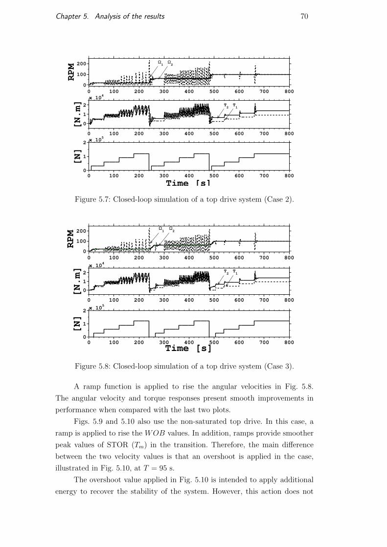
Chapter 5. Analysis of the results 70
0 100 200 300 400 500 600 700 8000
100
200
RPM
0 100 200 300 400 500 600 700 800
0
1
2
x 104
[N.m]
0 100 200 300 400 500 600 700 8000
1
2 x 10⁵
[N]
Time [s]
Ω1
Ω2
T2
T1
Figure 5.7: Closed-loop simulation of a top drive system (Case 2).
0 100 200 300 400 500 600 700 8000
100
200
RPM
0 100 200 300 400 500 600 700 800
0
1
2
x 104
[N.m]
0 100 200 300 400 500 600 700 8000
1
2 x 10⁵
[N]
Time [s]
Ω2
Ω1
T1
T2
Figure 5.8: Closed-loop simulation of a top drive system (Case 3).
A ramp function is applied to rise the angular velocities in Fig. 5.8.
The angular velocity and torque responses present smooth improvements in
performance when compared with the last two plots.
Figs. 5.9 and 5.10 also use the non-saturated top drive. In this case, a
ramp is applied to rise the WOB values. In addition, ramps provide smoother
peak values of STOR (Tm) in the transition. Therefore, the main difference
between the two velocity values is that an overshoot is applied in the case,
illustrated in Fig. 5.10, at T = 95 s.
The overshoot value applied in Fig. 5.10 is intended to apply additional
energy to recover the stability of the system. However, this action does not
DBD
PUC-Rio - Certificação Digital Nº 1612778/CA

Chapter 5. Analysis of the results 71
0 100 200 300 400 500 600 700 8000
100
200RPM
0 100 200 300 400 500 600 700 800
0
1
2
x 104
[N.m]
0 100 200 300 400 500 600 700 8000
1
2 x 10⁵
[N]
Time [s]
Ω1
Ω2
T1
T2
Figure 5.9: Closed-loop simulation of a top drive system (Case 4).
0 100 200 300 400 500 600 700 8000
100
200
RPM
0 100 200 300 400 500 600 700 800
0
1
2
x 104
[N.m]
0 100 200 300 400 500 600 700 8000
1
2 x 10⁵
[N]
Time [s]
T1
T2
Ω1
Ω2
Figure 5.10: Closed-loop simulation of a top drive system (Case 5).
reflect the effectiveness or the controlability of this system.
DBD
PUC-Rio - Certificação Digital Nº 1612778/CA

Chapter 5. Analysis of the results 72
5.4.2Proportional, integral and derivative controller (PID)
In this section, the linear PID controller is designed to improve the PI
response. However, it still does not mitigate completely the stick-pahse for a
grater range due to the nonlinearity characteristic of the problem. But the
controller has established a significant improvement to the drilling system
angular response.
Simulink models the PID based on the parameters of Tab. 5.1 and Tab.
5.5 and in the block diagram of Fig. 4.1. Then, the SSS of the system with
a PID controller is calculated as the first step to characterize this control
strategy, as shown in Fig. 5.4.2.
5.11(a): 3D map
RPM
WOB [kN]
20 40 60 80 100 120
20
40
60
80
100
120
140
160
180
200
0
10
20
30
40
50
60
70
80
90
100
5.11(b): 2D map
0 50 100 150 200−20
0
20
40
60
80
100
120
140
160
180
200
WOB [kN]
DR
PM
[R
PM
]
5.11(c): Ωref = 79, 36 rpm
0 20 40 60 80 100 120−20
0
20
40
60
80
100
120
140
160
180
200
Setpoint [RPM]
DR
PM
[R
PM
]
5.11(d): WOB = 160 kN
Figure 5.11: Calculated SSS and Bifurcation diagrams for PID controller.
The results in Fig 5.4.2 show that the stability transition region is
abruptly different when compared to the open-loop SSS color map for the
chosen criteria. However, if compared to the PI controller SSS curve the
difference is smooth.
Similarly to the PI SSS color map, the angular velocity around 80-90
rpm also represents a transition region where the oscillation become more
severe. A Hopf supercritical bifurcation diagram may show the amplitude of
vibration increasing when different WOB are applied to the current system.
Here, angular velocity of 80 rpm is adopted for future comparison with the
previous simulation. The results are illustrated in Fig. 5.11(c).
DBD
PUC-Rio - Certificação Digital Nº 1612778/CA

Chapter 5. Analysis of the results 73
Fig. 5.11(c) shows two bifurcation points that represent points where
the oscillatory behavior begins or becomes more severe. The first is around
WOB = 80 kN and the most severe, starts around WOB = 150 kN.
It may be noted from these results that PID controller will smoothly lose
operating window when compared to the PI controller.
Next,a constant WOB = 160 kN is chosen for further investigations on
the dynamic behavior of the downhole system, for a setpoint velocity range.
The bifurcation diagram compares donwhole and setpoint angular velocities,
as seen in Fig. 5.11(d).
It can be conclude that the gain of the derivative term does not strongly
affect the system when compared to the PI controller. Consequently, the system
is oscillating with peaks that are slightly larger than that shown in the previous
section (under the same conditions).
Thus, it is assumed the WOB = 80 kN acts under the conditions of
the friction torque modeling (Eq. 3-14) to simulate the nonlinearity bit-rock
interactions.
Although the configuration of the PID parameters has not been made
correctly for a nonlinear system, the parameters in the Tab. 5.5 are still being
used in these simulations. Thus, the numerical calculation is performed using
the angular velocities range of Tab. 5.2, as reference input signals. The time
domain results of the nonlinear system submitted to a linear compensator are
shown in Fig. 5.12.
0 20 40 60 80 100 1200
20
40
60
80
100
120
140
160
180
Time [s]
RPM
Ω2
5
4
3
2
1
Ω1
Figure 5.12: Nonlinear angular velocity responses for PID controller.
The stick-slip phenomenon may happen at low velocity and high WOB.
DBD
PUC-Rio - Certificação Digital Nº 1612778/CA

Chapter 5. Analysis of the results 74
Based on the simulations illustrated in Fig. 5.12 the system attributes are
displayed in Tab. 5.10.
Att. Ω1st1 Ω1st
2 Ω2nd1 Ω2nd
2 Ω3rd1 Ω3rd
2 Ω4th1 Ω4th
2 Ω5th1 Ω5th
2τr(s) 2.36 0.30 1.23 0.36 1.88 0.38 1.95 0.39 2.10 0.39τs(s) N/A 1.06 N/A 1.93 N/A 2.01 12.91 2.11 12.05 2.19τp(s) N/A 0.85 12.03 0.88 9.31 0.89 8.14 0.89 7.59 0.89
% OS 51.40 2.24 280.05 6.31 50.49 7.79 29.91 9.03 20.34 9.99
Table 5.10: Attributes of the drill string step responses with PID.
Thus, the attributes show that in the first three cases (1,2,3) there is
no settling time in the downhole Ω1 (the values are represented by N/A
[Not Applied]). Fig. 5.12 shows that for these three setpoints there is a non-
controlled oscillation that disturbs the system. However, if an angular velocity
Ωref > 80rpm is applied to the system, it begins to exhibit a less severe
behavior, or at least no oscillation.
A more detailed analysis is applied to the velocity of 26, 45 rpm (the
most severe case presented). The analysis shows the angular velocity behave
on the surface and in the drill-bit, the TOB and STOR, and the supply voltage
supplied by the PID controller, as seen in Fig. 5.13.
0 20 40 60 80 100 1200
20
40
60
RPM
0 20 40 60 80 100 1200
1
2 x 10⁴
N.m
0 20 40 60 80 100 1200
20
40
60
Time [s]
Volts
Ω2
Ω1
T2
T1
Figure 5.13: Nonlinear response of a PID Closed-loop system.
A comparison of the actual PID controller with the previous results
(undisturbed PID controller system in Figs. 5.3) shows a loss of quality
performance when the PID compensator is used in a nonlinear environment. An
unstable angular velocity response, an undamped system, and a slow velocity
response are observed, as seen in Fig. 5.13.
DBD
PUC-Rio - Certificação Digital Nº 1612778/CA

Chapter 5. Analysis of the results 75
Tab. 5.11 summarize the simulation performance responses. For example,
the maximum peak of the downhole angular velocity Ω1 increases from an
overshoot of 2.9% to a maximum of 51.3% of the reference value. However,
there is no steady state error and quick response when the controller is able
to mitigate the vibration. This confirms that the PID controller improves the
linear part of control system.
Drill stringNum. Ωref [Ω1 & Ω2]settled Ωmax
1 Ωmax2
1 26.45 rpm N/A 54.31 rpm 27.05 rpm
2 52.90 rpm N/A 95.33 rpm 56.03 rpm
3 79.36 rpm N/A 116.63 rpm 85.53 rpm
4 105.81 rpm 105.81 rpm 137.46 rpm 115.36 rpm
5 132.26 rpm 132.26 rpm 159.16 rpm 145.48 rpm
Table 5.11: Drill string with PID simulation performance.
DBD
PUC-Rio - Certificação Digital Nº 1612778/CA

Chapter 5. Analysis of the results 76
5.4.3Model predictive controller (MPC)
In this section, MPC is the control strategy used specifically to control
the nonlinear behavior of the system. For this reason, the MPC really intends
to mitigate the stick-slip phenomenon regarding the model complexity in the
drilling system.
As usual, the system parameters from Tab. 5.1 and the block diagram of
Fig. 4.1 are considered. In addition, a Simulink modeling is proposed. Thus,
the system color map SSS when subjected to the MPC is illustrated in Fig.
5.4.3.
5.14(a): 3D map
SRPM [RPM]
WO
B [
kN]
20 30 40 50 60 70 80 90 100 110 120
20
40
60
80
100
120
140
160
180
200
0
10
20
30
40
50
60
70
80
90
100
5.14(b): 2D map
0 50 100 150 200−20
0
20
40
60
80
100
120
140
160
180
200
WOB [kN]
DR
PM
[R
PM
]
5.14(c): Ωref = 79, 36 rpm
0 20 40 60 80 100 120−20
0
20
40
60
80
100
120
140
160
180
200
Setpoint [RPM]
DR
PM
[R
PM
]
5.14(d): WOB = 160 kN
Figure 5.14: Calculated SSS and Bifurcation diagrams for MPC controller.
The SSS color maps of the MPC drilling system show a totally new
behavior related to the stick-slip phenomenon. However, it is sensitive to the
criteria adopted, as seen in Fig. 5.4.3. In practice, the MPC controls the stick-
phase for the cases performed, but maintains the oscillations of steady state
with low amplitude in certain.
Further analyses indicated that the blue region corresponding to WOB
between 100 kN and 200 kN and at an angular reference speed between 20rpm and 50 rpm is the completely stopped angular velocity (in fact, velocities
are very close to zero).
The color map diagram shows a larger transition region when compared
to the previous two controllers. Therefore, among several angular velocity
DBD
PUC-Rio - Certificação Digital Nº 1612778/CA

Chapter 5. Analysis of the results 77
values in the transition region the Ωref = 80 rpm is a good option for later
comparison with previous cases
A Hopf supercritical bifurcation diagram may show the amplitude of
vibration increasing when different WOB are applied to the system with MPC
controller, as illustrated in Fig. 5.14(c).
Fig. 5.14(c) shows two bifurcation points. The first is around WOB =85 kN. The most severe starts around WOB = 115 kN. It may be noted from
this diagram that, as the WOB increases, the downhole velocity decreases.
This means that this controller does not maintain the speed at the desired
value but close to it.
Further investigation on the dynamic behavior of the downhole system, at
constant WOB = 160 kN and varying the setpoint velocity, generates another
bifurcation diagram. This diagram compares donwhole angular velocity and
setpoint angular velocity, as seen in Fig. 5.14(d).
Fig. 5.14(d) shows that at low velocity (from 20 rpm to 40 rpm) the
downhole angular velocity is zero. Then, oscillations start and increase in the
system until an angular velocity faster than 100 rpm. This behavior may change
as a different WOB value is chosen.
Simulations using MPC are performed for a system with nonlinearities.
For this, specific parameters were tuned using commercial software it Simulink.
Then, the numerical calculations are performed using the settled angular
velocity of Tab. 5.2, as reference input signal, and system parameters from
Tab. 5.1. The time domain results of the nonlinear compensated system are
presented in Fig. 5.15.
The system attributes, displayed in Tab. 5.12, are based on the simula-
tions performed in Fig. 5.15.
Att. Ω1st1 Ω1st
2 Ω2nd1 Ω2nd
2 Ω3rd1 Ω3rd
2 Ω4th1 Ω4th
2 Ω5th1 Ω5th
2τr(s) 2.20 0.54 2.37 16.64 2.50 23.27 2.59 19.34 2.98 19.52τs(s) N/A N/A 117.39 59.42 85.47 33.26 28.37 26.11 28.51 26.22τp(s) 21.24 1.56 16.10 28.57 13.41 36.86 11.99 87.85 90.26 87.85%OS 68.22 79.49 54.89 4.40 29.09 1.06 10.65 0.002 8.96e-4 0.002
Table 5.12: Attributes of the drill string step responses with MPC.
Thus, the attributes show that in the first two cases (1 and 2) there is
no settling time in the downhole Ω1. Fig. 5.15 shows that for these setpoints
there are non-controlled oscillations that disturb the system. However, if the
angular velocity Ωref > 80rpm is applied in the system, it begins to run without
oscillation, or at least it exhibits less severe vibrational behavior.
By choosing the most critical velocity of the results in Fig. 5.15 a
more effective study can be applied to the pre-determined reference velocity
DBD
PUC-Rio - Certificação Digital Nº 1612778/CA

Chapter 5. Analysis of the results 78
0 20 40 60 80 100 1200
20
40
60
80
100
120
140
Time [s]
RPM
Ω2
Ω1
5
4
3
2
1
Figure 5.15: Nonlinear angular velocity responses for MPC.
26, 45 rpm. Thus, the analysis consists in investigating the behavior of the
angular velocity of the surface and the downhole, the TOB and the STOR,
and the supply voltage, delivered by the MPC, as seen in Fig. 5.16.
0 20 40 60 80 100 1200
20
40
RPM
0 20 40 60 80 100 1200
1
2 x 10⁴
N.m
0 20 40 60 80 100 1200
20
40
Time [s]
Volts
Ω2
T2
T1
Ω1
Figure 5.16: Nonlinear response of a MPC Closed-loop system.
Current MPC responses in the time domain are compared to the PID
response in the undisturbed system (see Fig. 5.3). Thus, a long transient phase
until the system is stable means that the speed response becomes slow when
MPC is applied. The overshoot of the downhole angular velocity Ω1 increases
from 2.9% to 25% of the nominal value. Furthermore, there is a steady state
DBD
PUC-Rio - Certificação Digital Nº 1612778/CA

Chapter 5. Analysis of the results 79
error of about 25% of the nominal value for each setpoint velocity applied.
Drill stringNum. Ωref [Ω1 & Ω2]settled Ωmax
1 Ωmax2
1 26.45 rpm 19.79 rpm 33.29 rpm 35.52 rpm
2 52.90 rpm 46.26 rpm 71,62 rpm 48.29 rpm
3 79.36 rpm 72.68 rpm 93.82 rpm 73.47 rpm
4 105.81 rpm 96.06 rpm 106.30 rpm 96.07 rpm
5 132.26 rpm 117.98 rpm 117.98 rpm 117.98 rpm
Table 5.13: Drill string with MPC simulation performance.
DBD
PUC-Rio - Certificação Digital Nº 1612778/CA
Chapter 5. Analysis of the results 80
5.4.4MPC and PID controllers (MPC+PID)
Designed to improve the behavior of the MPC (alone), this combined
control strategy (MCP+PID) is used not only to control the nonlinearity of
the system, but also to correct the equilibrium error observed in the last system.
Thus, this strategy mitigates the stick-slip phenomenon under some conditions.
In fact, it improves the characteristics of the drilling system by defining a better
operating window.
All the simulations are based on system parameters from Tab. 5.1 and
the block diagram of Fig. 4.1. A Simulink modeling is designed to simulate the
dynamic drilling system with a motor actuator. The torsional vibration map
of the drill string system when subjected to MPC+PID is illustrated in Fig.
5.4.4.
5.17(a): 3D map
RPM
WOB [kN]
20 40 60 80 100 120
20
40
60
80
100
120
140
160
180
200
0
10
20
30
40
50
60
70
80
90
100
5.17(b): 2D map
0 20 40 60 80 100 120 140 160 180 200
0
50
100
150
200
WOB [kN]
DR
PM
[R
PM
]
5.17(c): Ωref = 79, 36 rpm
0 20 40 60 80 100 1200
20
40
60
80
100
120
140
160
180
200
Setpoint [RPM]
DRPM [RPM]
5.17(d): WOB = 100 kN
Figure 5.17:
In this case, also, it is possible to say that the angular velocity around
80 rpm represents a transition region where the oscillation has become more
severe. A Hopf supercritical bifurcation diagram can show the amplitude of
vibration increasing when different WOB are applied to the system with
MPC+PID controller, as illustrated in Fig. 5.17(c).
In Fig. 5.17(c) two points of bifurcation are observed. The first is around
WOB = 90 kN and the most severe is around WOB = 160 kN. However,
investigations are proposed on the dynamic behavior of the downhole system
DBD
PUC-Rio - Certificação Digital Nº 1612778/CA

Chapter 5. Analysis of the results 81
for the constant WOB = 100 kN and a setpoint velocity range. Therefore, the
bifurcation diagram that compares the donwhole angular velocity and setpoint
angular velocity is created, as seen in Fig. 5.17(d).
The general behavior of the nonlinear drilling system, illustrated in Fig.
5.4.4, evaluates the effectiveness of the combined MPC+PID control in the
system. Furthermore, simulations are performed for a system with nonlinearity
and some parameters are tuned to use in the MPC block diagram. The
numerical calculations are performed using the range of angular velocity of
Tab. 5.2, as reference input signal. The time domain results of the combined
nonlinear compensator (MPC+PID) are shown in Fig. 5.18.
0 20 40 60 80 100 1200
20
40
60
80
100
120
140
160
180
Time [s]
RPM
1
Ω1
Ω2
5
4
3
2
Figure 5.18: Nonlinear angular velocity responses for MPC+PID controller.
Att. Ω1st1 Ω1st
2 Ω2nd1 Ω2nd
2 Ω3rd1 Ω3rd
2 Ω4th1 Ω4th
2 Ω5th1 Ω5th
2τr(s) 2.17 0.49 2.21 1.02 2.29 9 11.56 2.48 11.29 3.03 11.32τs(s) 89.73 70.96 86.25 68.97 71.85 8 70.36 72.53 70.14 72.43 70.04τp(s) 17.04 1.65 13.59 16.68 11.96 22.71 26.72 24.71 27.66 25.69%OS 79.05 120.13 66.77 21.70 32.11 16.48 14.67 14.70 13.80 13.84
Table 5.14: Attributes of the drill string step responses with MPC+PID.
A specific analysis, using the critical results of Fig. 5.12, is performed
to generate stick-slip phenomenon for low velocity and high WOB. Thus,
studies are done for setpoint velocity of 26, 45 rpm. The analysis consists of
investigating the behavior of the angular velocity at the surface and the drill-
bit, the TOB and the STOR, and supply voltage delivered by the controller,
as seen in Fig. 5.19.
DBD
PUC-Rio - Certificação Digital Nº 1612778/CA

Chapter 5. Analysis of the results 82
0 20 40 60 80 100 1200
20
40
60
RPM
0 20 40 60 80 100 1200
1
2 x 10⁴
N.m
0 20 40 60 80 100 1200
20
40
Time [s]
Volts
Ω2
Ω1
T1
T2
Figure 5.19: Nonlinear response of a MPC+PID Closed-loop system.
The time domain responses of the combined MPC+PID control are
compared to the response of the nonlinear MPC and of the linear PID
controllers, separately. In addition, the current controller is compared to the
undisturbed PID controller, seen in Fig. 5.3.
Thus, MPC+PID performance enhancements show that the PID compo-
nent (of the combined system) is responsible for a long transient phase until
the system has stabilized and the MPC component is responsible for compen-
sating system nonlinearity. For this reason, both systems should be tuned with
different parameters than those used in previous sections. The first overshoot
of the downhole angular velocity Ω1 are betweeen 15% to 25% of the nominal
value. Furthermore, there is no steady state error of the nominal value for the
chosen setpoint velocities.
Drill stringNum. Ωref [Ω1 & Ω2]settled Ωmax
1 Ωmax2
1 26.45 rpm 26.45 rpm 47.37 rpm 58.23 rpm
2 52.90 rpm 52.90 rpm 88.23 rpm 64.38 rpm
3 79.36 rpm 79.36 rpm 104.84 rpm 92.43 rpm
4 105.81 rpm 105.81 rpm 121.33 rpm 121.37 rpm
5 132.26 rpm 132.26 rpm 150.52 rpm 150.57 rpm
Table 5.15: Drill string with MPC + PID simulation performance.
DBD
PUC-Rio - Certificação Digital Nº 1612778/CA

6General conclusions and future works
6.1Conclusions
Recalling that in the current industry overview presented in Section
1.1, the major interest of the drilling industry is to improve operational
performance and reduce overall operating costs. Among several approaches in
that order, the reduction or elimination of stick-slip vibration is an important
step in that direction.
Note that in the literature (see Section 2.2) it is possible to find numerous
studies related to stick-slip and control topics. However, when looking at the
industry, there is not an ultimate model or methodology used in a practical
way. Therefore, it is not an overestimation of this study to attempt to initiate
such an approach.
Taking the last paragraph in mind, the author stated that the main
objective of this dissertation is to minimize the problem of torsional vibration
of the drill bit using existing control strategies. Also, he considers evaluation
and confronting the performance of the strategies.
The main objective is subdivided into five research objectives. First,
the development of an open-loop analysis of the drilling system considering
a saturated and a non-saturated top drive actuator; second, the application
of existing control strategies using different torque/velocity inputs in a closed-
loop system; third, it is considered the control of the torsional vibration with
nonlinearity due to friction interaction with the wall and in the donwhole
system; fourth, it intends to evaluate a non-stop control system while drilling,
fifth, it intends to implement the improvements of the model in an experimental
reduced setup for future verification and validation of the models.
The main contributions of this dissertation addressing these objectives
can be summarized in terms of contributions on the development of an open-
loop methodology to decouple the actuator and the plant, on the application
of a wide range of inputs to optimize the output of the controller (supply
voltage), on controlling the stick-slip with nonlinearity due to friction in the
downhole system, on the evaluation of the controller performances during
DBD
PUC-Rio - Certificação Digital Nº 1612778/CA

Chapter 6. General conclusions and future works 84
drilling operation.
– The development of an open-loop methodology to decouple the actuator
and the plant: One of the great contributions of this study is part of the
control design methodology proposed in Chapter 4. Opening the loop of
the closed-loop system, with motor actuator and drill string, proved to
be extremely useful in understanding the behavior of the system. The
response of the open-loop drill string system provided an angular velocity
related to an imposed torque. With this information, it is possible to
define the appropriate top drive unit for each demand. Moreover, when
applying a wide range of inputs combined with the open-loop drill string
responses in the open-loop DC motor, the basis to optimize the output
of the controller is provided.
– The application of a wide range of inputs to optimize the output of the
controller (supply voltage): The steps of the interactive open-loop method
for analysis are presented in Chapter 5. The results of the Section 5.2
showed the open-loop response to the imposed inputs and the optimized
supply voltage. This information is important when the signal that would
be controlled has to be chosen. It is also helpful to identify which control
law should be used.
– Controlling the stick-slip with nonlinearity due to friction in the downhole
system: Initially (in Section 4.4), a linear method was used to compensate
the torsional vibrations in the drilling system. The conventional PI rotary
speed control method attenuated and reduced torsional vibration under
certain conditions. However, if the characteristics of the system change, it
is only efficient when the goal is to keep the angular velocity almost stable
around a set point (as in Chapter 5). So, for the linear PI control law to
be defined for the disturbance generated by the stick-slip phenomena, its
parameters (proportional and integral gain) must be chosen intelligently.
Tucker & Wang (2003) [11] demonstrated in their study an efficient way
to choose PID parameters. It is also possible to follow an orientation for
automatic speed controller tuning on paper [58]. But, as applied here, the
torque response generated by nonlinearity shows that this friction torque
can not be efficiently compensated only by using a linear control. A robust
nonlinear controller must be applied to work in conjunction with the PI
rotary speed controller.
That is why the use of a model-based control is one of the most relevant
actions in this study. Although the limitations found in the adopted model
and settings, it is clear the powerful tool this strategy has proven to
be. It was able to confront the nonlinear behavior of the system. It also
DBD
PUC-Rio - Certificação Digital Nº 1612778/CA

Chapter 6. General conclusions and future works 85
controlled and improved other control actions for the set of settings used.
Due to the limitations to properly define the parameters for this, this
strategy was not able to control the nonlinearity and maintain the angular
velocity by itself. But in combination with the PID controller proved to
be a robust strategy.
– The evaluation of the controller performances during drilling operation:
Some of the main contributions of this work are, first, the fact that
it was done on a real-scale configuration with the top drive system
as the actuator. This indicates that the hardware configuration can be
constructed using these parameters as the basis.
The simulation proves that speed feedback control is needed, but not
enough to cure the stick-slip. The speed controller is one way to achieve
the driller’s needs to keep the angular velocity as stable as possible.
The bit-torque friction model used in the initial simulation represents the
observed behavior of the torsional system. Once the systems are stabilized,
the oscillation generated by the stick-slip phenomenon are reduced. Thus,
we can conclude that the oscillations of the system reduce their velocity
amplitude while the motor speed increases.
6.2Recommendations for future research
In this final section, recommendations for future research directions are
given. First, two general recommendations for future research are presented on
the control theory presented in Section 2.3.1. In this section,the basic concepts
of control applied in the oil and gas industry were presented.
– Development of new controller design strategies: The controller design
strategies proposed in this study should consider the active surface control
of the drilling system considering the conventional and model-based
approach.
– Robustness analysis, verification and validation on a experimental reduced
drill-string setup: The reduced drilling string configuration has already
been developed and validated for a dynamic model in the Dynamics and
Vibration Laboratory of the Mechanical Engineering Department of PUC-
Rio. The next steps are the implementation of existing control strategies
on the test rig.
– Development of an optimization of control parameters: The optimization
of the control parameters is essential for this project, since the parameters
used in this study were reached by an error and trial methodology to
DBD
PUC-Rio - Certificação Digital Nº 1612778/CA

Chapter 6. General conclusions and future works 86
approximate the optimized supply voltage. Parameters must be optimized
every time the physical system settings change.
– Controller in real time: It is interesting to also investigate if controllers can
be used in a real-time implementation. Thus, the next step of the project
is to implement the control strategy mentioned in the methodology to
investigate the situations mentioned.
Afterward, a torsional stability diagram of the drilling process should
be drawn to better understand which variables influence the stability of the
system, and then a system with the best way to mitigate the stick-slip should
be developed.
– Apply different models of bit-rock friction: Analyze and perform simula-
tions considering different models of bit-rock friction. This may help to
better represent the behavior of the bit-rock interaction, given by the
friction model. The fact is that the different friction models can represent
different situations of the bit-rock interactions or of the drill pipe-wall
interaction.
– Experimental validation of friction models: Among these different friction
models it is possible to choose which one obtains superior empirical results
during the drilling process. It should be remembered that the drilling
process is not a singular behavior because it could change, for example,
due to the variation of the load, lubrication and roughness of the surface
(nature of the rocks). Thus, it is interesting to apply the control design
to the different situations that have been defined.
Based on the presented methodology other configurations of the system
parameters will be applied in the drilling system to analyze its behavior
when applying different controllers. Settings such as drill string length, DOF
numbers, WOB,Ωref , will be changed in future studies in the next phase of the
work.
DBD
PUC-Rio - Certificação Digital Nº 1612778/CA

Bibliography
[1] E. M. Navarro-Lopez,“Bit-sticking Phenomena in a Multidegree-of-
freedom Controlled drill string,” in Exploration & Production, vol. 8 of
2, pp. 70–75, 2010.
[2] D. E. Seborg, T. F. Edgar, and D. A. Mellichamp, Process Dynamics and
Control. New Jersey: Jonh Wiley and Sons, Inc., 2nd ed., 2004.
[3] M. I. Khan, T. Yasmeen, A. Shakoor, N. B. Khan, and R. Muhammad,“2014
oil plunge: Causes and impacts on renewable energy,”in Renewable
and Sustainable Energy Reviews, vol. 68, pp. 609–622, 2017.
[4] Bonaire Le - Nexant, “Crude-oil’s impact on renewable energy:
energy alternative or energy staple?.” Online; accessed 08-Feb,
2017. http://www.altenergymag.com/article/2015/06/crude-oil’s-impact-
on-renewable-energy-energy-alternative-or-energy-staple/20384/.
[5] C. Handscom, S. Sharabur, and J. Woxholth, “The oil and gas
organization of the future.” Online; accessed 08-Feb, 2017.
http://www.mckinsey.com/industries/oil-and-gas/our-insights/the-oil-
and-gas-organization-of-the-future.
[6] L. Van den Steen, Suppressing Stick-Slip-Induced drill string Oscil-
lations: A Hyperstability Approach. PhD thesis, University of Twente,
Enschede, The Netherlands, 1997.
[7] A. F. A. Serrarens,“H∞ Control as Applied to Torsional drill string
Dynamics,”Master’s thesis, Eindhoven University of Technology, Eindhoven,
The Netherlands, 1997.
[8] P. Sananikone, O. Karnoshirna, and D. B. White, “A Field Method for
Controlling drill string Torsional Vibrations,” in IADC/SPE Drilling
Conference, SPE-23891, (New Orleans, Louisiana), pp. 443–452, February
1992.
[9] F. Abdulgalil and H. Siguerdidjane,“PID Based on Sliding Mode Con-
trol for Rotary Drilling System,”in IEEE/EUROCON The International
Conference on ”Computer as a Tool”, vol. 2, (Serbia & Montenegro, Belgrade),
pp. 262–265, November 2005.
DBD
PUC-Rio - Certificação Digital Nº 1612778/CA

Bibliography 88
[10] A. H. Suleiman, “Modeling of Stick-Slip Drillstring Vibration in
Oilwell Drilling Operation,” tech. rep., Universiti Teknologi MARA
(UiTM), Selangor Darul Ehsan, Malaysia, 2006.
[11] R. W. Tucker and C. Wang, “Torsional Vibration Control and
Cosserat Dynamics of a Drill-Rig Assembly,” in Meccanica, vol. 38,
pp. 143–159, 2003.
[12] A. Yigit and A. Christoforou,“Coupled Torsional and Bending Vibra-
tions of Drillstrings Subject to Impact with Friction,” in Journal
of Sound and Vibrations, vol. 215(1), pp. 167–181, 1998.
[13] T. G. Ritto and R. Sampaio, “Measuring the efficiency of vertical
drill-string: A vibration perspective,”in Mechanics Research Commu-
nications, vol. 52, pp. 32–39, 2013.
[14] F. Abdulgalil and H. Siguerdidjane,“Nonlinear Friction Compensation
Design for Suppressing Stick Slip Oscillations in Oil Well drill
strings,” in 7th IFAC DYCOPS, (Massachusets, USA), July 2004.
[15] P. C. Kriesels, W. J. G. Keultjes, P. Dumont, I. Huneidi, O. O. Owoeye, and
R. A. Hartmann,“Cost Savings through an Integrated Approach to
drill string Vibration Control,” in SPE/IADC Middle East Drilling
Technology Conference, SPE-57555, (Abu Dhabi, United Arab Emirates),
November 1999.
[16] G. W. Halsey, A. Kyllingstad, and A. Kylling, “Torque Feedback Used
to Cure Slip-Stick Motion,” in 63rd Annual Technical Conference and
Exhibition of the Society of Petroleum Engineers, (Houston, TX), pp. 277–
282, October 1988.
[17] M. B. Saldivar, S. Mondie, and J. J. Loiseau, “Reducing Stick-Slip
Oscillations in Oilwell drill strings,”in 6th International Conference on
Electrical Engineering, Computing Science and Automatic Control, (Toluca
de Lerdo, Mexico), pp. 1–6, Jan. 2009.
[18] M. Karkoub, M. Zribi, L. Elchaar, and L. Lamont, “Robust µ-synthesis
controllers for suppressing stick-slip induced vibrations in oil
well drill strings,” in Multibody System Dynamics - Springer, vol. 23,
pp. 191–207, 2010.
[19] R. B. Jijon, C. Canudas-de-Wit, S. Niculescu, and J. Dumon, “Adaptive
Observer Design under Low Data Rate Transmission with Ap-
plications to Oil Well Drill-string,” in American Control Conference,
(Baltimore, Maryland), July 2010.
DBD
PUC-Rio - Certificação Digital Nº 1612778/CA

Bibliography 89
[20] G. Dong and P. Chen, “A Review of the Evaluation, Control, and
Application Technologies for Drill String Vibrations and Shocks
in Oil and Gas Well,” in Shock and Vibration, vol. 2016, p. 7418635,
2016.
[21] X. Zhu, L. Tang, and Q. Yang, “A Literature Review of Approaches
for Stick-Slip Vibration Suppression in Oilwell Drillstring,” in
Advances in Mechanical Engineering, vol. 6, p. 967952, 2014.
[22] K. Javanmardi and D. T. Gaspard, “Soft Torque Rotary System Re-
duces Drillstring Failures,” in Oil & Gas Journal, vol. 90 of 41, 1992.
[23] K. Javanmardi and D. T. Gaspard,“Application of Soft-Torque Rotary
Table in Mobile Bay,” in IADC/SPE Drilling Conference, SPE-23913,
(New Orleans, Louisiana), pp. 645–650, October 1992.
[24] R. N. Worrall, I. P. J. M. Stulemeijer, J. D. Jansen, and B. G. G. Van Wal-
stijn, “Method and system for controlling vibrations in borehole
equipment.” United States Patent, No. US 5117926, June 1992.
[25] J. D. Jansen and L. van den Steen, “Active Damping of Self-Excited
Torsional Vibrations in Oil Well Drillstrings,” in Journal of Sound
and Vibration, vol. 179 of 4, pp. 647–668, 1995.
[26] J. D. Jansen, L. van den Steen, and E. Zachariasen, “Active Damping of
Torsional Drillstring Vibrations With a Hydraulic Top Drive,”in
European Petroleum Conference, (London), pp. 250–254, October 1995.
[27] R. W. Tucker and C. Wang, “On the Effective Control of Torsional
Vibrations in Drilling Systems,” in Journal of Sound and Vibration,
vol. 224, pp. 101–122, 1999.
[28] F. Abdulgalil and H. Siguerdidjane,“Backstepping Design for Control-
ling Rotary Drilling System,” in IEEE Conference on Control Applica-
tions, (Toronto, Canada), pp. 120–124, August 2005.
[29] C. Canudas-de-Wit, J. Aracil, F. Gordillo, and F. Salas, “The Oscillations
Killer: a Mechanism to Eliminate Undesired Limit Cycles in
Nonlinear Systems.,” tech. rep., Grenoble INP, Grenoble, France, 2005.
[30] C. Canudas-de-Wit, M. A. Corchero, F. R. Rubio, and E. M. Navarro-Lopez,
“D-OSKIL: a New Mechanism for Suppressing Stick-Slip in Oil
Well Drill Strings,” in 44th IEEE Conference on Decision and Control,
(Seville, Spain), pp. 8260–8265, December 2005.
[31] M. A. Corchero, C. Canudas-de-Wit, and F. R. Rubio, “Stability of the
D-OSKIL Oscillation Suppression Mechanism for Oil Well Drill-
DBD
PUC-Rio - Certificação Digital Nº 1612778/CA

Bibliography 90
strings,”in 45th IEEE Conference on Decision & Control, (San Diego, USA),
pp. 1846–1851, December 2006.
[32] C. Canudas-de-Wit, F. R. Rubio, and M. A. Corchero,“D-OSKIL: A New
Mechanism for Controlling Stick-Slip Oscillations in Oil Well
Drillstrings,” in IEEE Transactions on Control System Technology, vol. 16
of 06, pp. 1177–1191, 2008.
[33] C. Canudas-de-Wit, J. Aracil, F. Gordillo, and F. Salas, “The Oscillations
Killer: a Mechanism to Eliminate Undesired Limit Cycles in a
Class of Nonlinear Systems,” in International Journal of Robust and
Nonlinear Control, 2008.
[34] E. M. Navarro-Lopez and D. Cortes, “Sliding-mode control of a multi-
DOF oilwell drillstring with stick-slip oscillations,” in The 2007
American Control Conference, (New York City, USA), July 11-13 2007.
[35] M. Karkoub, Y. L. Abdel-Magid, and B. Balachandran, “Drill-String Tor-
sional Vibration Suppression Using GA Optimized Controllers,”
in Journal of Canadian Petroleum Technology, vol. 48 of 12, pp. 32–38, 2009.
[36] Z. Qi-zhi, H. Yu-yao, L. Lin, and R. Nurzat, “Sliding Mode Control
of Rotary Drilling System With Stick Slip Oscillation,” in 2010
2nd International Conference on Computer Engineering and Technology,
(Chengdu, China), April 16-18 2010.
[37] Z. Qi-zhi, H. Yu-yao, L. Lin, and R. Nurzat,“A Double Surfaces Sliding
Mode Control Technique in Rotary Drilling System,” in 2010
2nd International Conference on Computer Engineering and Technology,
(Chengdu, China), April 16-18 2010.
[38] S. Fubin, S. Linxiu, L. Lin, and Z. Qizhi, “Adaptive PID Control of
Rotary Drilling System with Stick Slip Oscillation,” in 2010 2nd
International Conference on Signal Processing Systems (ICSPS), (Chengdu,
China), pp. 289–292, July 5-7 2010.
[39] H. Puebla and J. Alvarez-Ramirez, “Suppression of stick-slip in drill-
strings: A control approach based on modeling error compensa-
tion,” in Journal of Sound and Vibration, vol. 310, pp. 881–901, 2008.
[40] M. K. Johannessen and T. Myrvold, “Stick-Slip Prevention of Drill
Strings Using Nonlinear Model Reduction and Nonlinear Model
Predictive Control,”Master’s thesis, Norwegian University of Science and
Technology, Trondheim, Norway, 2010.
[41] P. Sananikone, O. Karnoshirna, and D. B. White, “A Field Method for
Controlling drill string Torsional Vibrations,” in SPE Americas: Un-
DBD
PUC-Rio - Certificação Digital Nº 1612778/CA

Bibliography 91
conventional Resources Conference, SPE-158109, (Pittsburgh, Pennsylvania),
pp. 443–452, July 2012.
[42] T. G. M. Vromen, Control of stick-slip vibrations in drilling sys-
tems. PhD thesis, Eindhoven University of Technology, Eindhoven, The
Netherlands, 2015.
[43] K. J. Astrom and T. Hagglund, PID Controllers: Theory, Designing,
and Tuning. Instrument Society of America, 2nd ed., 1994.
[44] M. A. P. L. Falb, Optimal Control: An Introduction to the Theory
and Its Applications. New York: McGraw-Hill, Inc., 1st ed., 2004.
[45] A. G. Mutambara, Design and Analysis of Control Systems. Florida:
CRC Press LLC, 2nd ed., 1999.
[46] K. Ogata, Modern Control Engineering. New Jersey: Prentice-Hall,
Inc., 3rd ed., 1997.
[47] J. D. Jansen, Nonlinear Dynamics of Oilwell Drillstrings. PhD thesis,
Delf University, Delf, The Netherlands, 1993.
[48] Electronics Tutorials, “Open-loop System and Open-loop Con-
trol Systems.” Online; accessed 12-Jan”
2017. http://www.electronics-
tutorials.ws/systems/open-loop-system.html.
[49] A. Ghasemloonia, D. Rideout, and S. D.Butt,“A review of drillstring vi-
bration modeling and suppression methods,”in Journal of Petroleum
Science and Engineering, vol. 131, pp. 150–164, 2015.
[50] Electronics Tutorials, “Closed-loop System and Closed-loop Con-
trol Systems.” Online; accessed 12-Jan, 2017. http://www.electronics-
tutorials.ws/systems/closed-loop-system.html.
[51] A. Sassan and B. Halimberdi,“Design of a Controller for Suppressing
the Stick-slip Oscillations in Oil well Drillstring,”in Research Journal
of Recent Sciences, vol. 2(6), pp. 78–82, 2013.
[52] B. Cayres, “Numerical and Experimental Analysis of Nonlinear
Torsional Dynamics of a Drilling System,”Master’s thesis, Pontificia
Universidade Catolica do Rio de Janeiro, Rio de Janeiro, Brazil, 2013.
[53] C. Germay, N. Van de Wouw, H. Nijmeijer, and R. Sepulchre, “Nonlinear
Drillstring Dynamics Analysis,” in Society for Industrial and Applied
Mathematics Journal, vol. 8 of 02, pp. 527–553, 2009.
[54] C. Canudas-de-Wit, K. J. A. H. Olsson, and P. Lischinsky, “A New Model
for Control of Systems with Friction,” in IEEE Transactions on
Automatic Control, vol. 40 of 03, pp. 419–425, 1995.
DBD
PUC-Rio - Certificação Digital Nº 1612778/CA

Bibliography 92
[55] N. Mihajlovic, A. A. van Veggel, N. van de Wouw, and H. Nijmeijer,
“Analysis of Friction-Induced Limit Cycling in an Experimental
Drill-String System,” in Journal of Dynamic Systems, Measurement, and
Control, vol. 126, pp. 709–720, 2004.
[56] J. F. Brett, “The Genesis of Torsional drill string Vibrations,” in
SPE/IADC Drilling Conference, SPE-21943, (Amsterdam, The Netherland),
pp. 168–174, September 1992.
[57] E. M. Navarro-Lopez, “Practical approach to modeling and control-
ling stick-slip oscillations in oilwell drill strings,” in International
Conference on Control Applications, (Taipei, Taiwan), September 2-4 2004.
[58] A. Kyllingstad and P. J. Nessjoen, “A New Stick-Slip Prevention
System,” in SPE/IADC Middle Drilling Conference and Exhibition ,
SPE-119660, (Amsterdam, The Netherlands), March 2009.
DBD
PUC-Rio - Certificação Digital Nº 1612778/CA