Lending on hold: Regulatory uncertainty and bank lending ...

Lending on hold: Regulatory uncertainty

and bank lending standards

Stefan Gissler, Jeremy Oldfather, and Doriana Ruffino ∗

October 2015

Abstract

Does higher regulatory uncertainty constrain credit? This paper focuseson the recent regulation of “qualified mortgages” (QM) and on the effectsof the related rule-making process on bank lending. In 2011, the FederalReserve proposed a set of criteria that would give lenders the presumption ofa borrower’s ability-to-repay a mortgage–and, thus, legal protection should aborrower sue. But the debt-to-income (DTI) ratio criterion–the most bindingin the final rule–was not specified in the proposed rule. The absence of such abright line created high regulatory uncertainty for banks between the proposedand the final rule. Using public comments submitted by banks in response tothe rule proposal, we compute a measure of policy uncertainty at the banklevel. We show that more uncertain banks issued fewer loans (and for smalleramounts) after the rule proposal. To control for general economic uncertainty,we instrument our measure by a bank’s past legal costs. We confirm thatbanks that historically were sued more often cut lending more severely duringthe rule-making process. At a more aggregated level, counties that recorded alarge number of mortgage lawsuits also experienced lower house price growth.

∗Gissler, Oldfather, and Ruffino are at the Federal Reserve Board. E-Mails: [email protected], [email protected], [email protected]. This article repre-sents the views of the authors, and should not be interpreted as reflecting the views of the Boardof Governors of the Federal Reserve System or other members of its staff.

1

1 Introduction

Does higher regulatory uncertainty constrain credit? A growing body of literature

suggests that uncertainty has real effects for the economy–for example, it may in-

crease firms’ cost of capital and decrease investment (Gilchrist, Sim, and Zakrajsek

2014). Investment might be forgone entirely if uncertainty hinders the decision-

making process of corporate boards (Garlappi, Giammarino, and Lazrak 2013). In

addition to these supply-side effects, high uncertainty dampens consumers’ demand

for goods and services in a downturn. During the Great Depression, a large drop

in consumption was associated with high uncertainty (Romer 1990). High uncer-

tainty may cause consumers to be more cautious, for example when purchasing a

car (Eberly 1994).

Government interventions and regulatory policies are leading sources of un-

certainty. Fernandez-Villaverde, Guerron-Quintana, Kuester, and Rubio-Ramırez

(2015) show how fiscal uncertainty about the timing and form of budgetary adjust-

ments reduces investment, employment, and consumption. Baker, Bloom, and Davis

(2013) link the slow recovery from the Great Recession to higher policy uncertainty

during the period 2007 to 2009. But while these papers show that expectations over

future policy changes do affect economic agents’ current decisions—an argument

made famous by Lucas (1976) and Kydland and Prescott (1977)—it has proven

difficult to disentangle the effects of policy uncertainty from other macroeconomic

factors. Furthermore, uncertainty is unobservable, objectively unmeasurable, and

may itself induce policy changes so that any inference must deal with the problem

of reverse causality.

In this paper we assess how uncertainty about mortgage regulations affected

bank lending and house prices. Between 2011 and 2014, the Consumer Financial

Protection Bureau (CFPB) proposed and implemented laws setting minimum re-

quirements for mortgage lenders to consider before extending credit to consumers.

In January 2013, the CFPB established a set of criteria for “qualified mortgages”

(QM). By fulfilling these requirements, a lender proves a borrower’s ability to repay

2

a loan and, in return, receives legal protection. This “safe harbor” significantly

reduces a creditor’s costs and risks of issuing a loan. Among these criteria is a

borrower’s monthly debt-to-income (DTI) ratio of 43 percent or less. Although the

proposed rule of May 2011 listed the DTI ratio among other criteria, it did not

specify a precise ratio. This absence of a bright line during the “due process of

the law” created high uncertainty about the CFPB’s final determination in the 18

months leading up to the final rule. Lenders guessed that the DTI standard even-

tually would be set between 36–the maximum back-end DTI proposed for qualified

residential mortgages (QRM)–and 43–the Federal Housing Administration’s (FHA)

underwriting standard.

Using differences in regulatory uncertainty across banks, we study how opacity

on QM criteria affected bank lending. To measure regulatory uncertainty, we search

for “uncertainty words” in the text of over 2,500 public comment letters submit-

ted by large banks and credit unions after each step of the rule development. Our

search shows that policy uncertainty varied greatly across lenders. When matched

with loan and borrower characteristics by lender, this result allows us to investigate

differential changes in housing credit.

Figure 1 summarizes our findings on aggregate changes in credit. It compares

the share of loans most likely affected by policy uncertainty–loans with DTI ra-

tios greater than 36 and lower than 44–with the safest loans to be originated–loans

with DTI ratios below 21. At the time of uncertainty about the QM definition (be-

tween the red vertical lines), the share of 37-43 DTI loans plummeted 6 percent.

Meanwhile, the share of loans with DTI ratios below 21 rose by 12 percent. As

uncertainty was resolved by the publication of the final rule, the dynamics of the

shares reverted.1 Our main results confirm these findings at the bank level.

Making use of our comment-based measure of uncertainty, we find that if a bank

1Interestingly, policy uncertainty appears to have an immediate effect on portfolio composition:the share of 37-43 DTI declines–and the share of loans with DTI ratios below 21 increases–atthe time of the rule proposal (the left vertical bar). Anecdotal evidence suggests that the costsof adjusting a banks underwriting model, including, for example, the updating of its informationsystem, are high enough to prompt a bank to act quickly in anticipation of the final rule.

3

perceives higher uncertainty than other banks, or if it is more adverse to uncertainty

than other banks, it is less likely to issue loans with DTI ratios between 37 and 43

prior to publication of the final rule. We also find that more uncertain banks is-

sue fewer loans: a one standard deviation increase in uncertainty reduces a bank’s

total monthly originations by 1.57 standard deviations. We obtain these results

from a large sample of banks, including banks that did not submit a comment on

the proposed rule. However, when we restrict the sample to banks that submitted a

comment, the results persist. This way, we address the potential concern that banks

that submitted a comment might differ from banks that did not.

Another concern is that our uncertainty measure may largely reflect general un-

certainty about a bank’s future outlook or business environment. We correct this

bias through banks’ historical legal costs. We reason that the “safe harbor” legal

protection granted under the QM rule is more valuable to banks that have histori-

cally incurred higher legal costs. To estimate these costs, we collect data from the

Public Access to Court Electronic Records (PACER) on court cases opened before

the recent housing boom and bust. In particular, we instrument policy uncertainty

by the number of lawsuits on the subject “Truth in Lending Act” that were ter-

minated before 2004. Banks (defendants) that historically were sued more often

displayed higher uncertainty during the rule-making process between 2011 and 2013

and a larger reduction in lending.

Our estimation strategy allows us to address several identification concerns.

First, since the banking sector as a whole might influence the policy making process,

we use variation across banks to identify the differential impact of uncertainty on

lending. Second, our natural experiment is sufficiently specific to only affect the

bank lending channel.2 By controlling for borrower, lender, and geographical char-

acteristics we can exclude other channels through which policy uncertainty might

affect bank lending.

2In contrast, higher uncertainty about oil prices might affect the behavior of several agentsin the economy. Thus, identifying the transmission channel from higher uncertainty to economicoutcomes is more arduous.

4

Since our results rely on the assumption that banks were uncertain about the

future regulatory DTI ratio, we revisit our uncertainty measure to show that it well

summarizes banks’ sentiment toward the DTI criterion. We uncover hidden topics

in bank comments and find that the DTI ratio was the prevalent topic. Further,

uncertainty remained high and stable throughout the rule-making process and was

resolved at once when the final rule was announced.

We end our analysis by investigating the effect of policy uncertainty on house

prices. We show that there exists a correlation between policy uncertainty (instru-

mented by bank lawsuits) and house prices at the county level. In particular, after

the rule proposal, credit was cut more severely in counties that recorded a larger

number of mortgage lawsuits. In these counties house prices grew less or declined

more than in other counties. Athough more work remains to be done to test and

establish the macro-economic effects of policy uncertainty, we provide some evidence

that regulatory indecision had (unintended) consequences on both lending and house

prices.

Our contribution to past research is threefold. First, we measure the differential

effect of policy uncertainty on bank lending—bypassing the issue of reverse causality

common to the literature on macroeconomic uncertainty. Second, we provide a de-

tailed study of credit cycles that originated solely from prolonged policy uncertainty.

Last, we show that counties that perceived higher policy uncertainty saw a larger

decline in lending and house prices.

Section 2 reviews past research relevant to our study. Section 3 provides detailed

background information on the QM regulatory framework. Section 4 describes the

data. Results on the composition and size of banks’ mortgage portfolios are pre-

sented in section 5. Section 6 shows that these results are robust to endogeneity and

other concerns. Section 7 introduces the geographical analysis and relates policy

uncertainty to changes in house prices. Section 8 concludes.

5

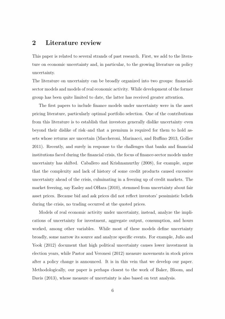
2 Literature review

This paper is related to several strands of past research. First, we add to the litera-

ture on economic uncertainty and, in particular, to the growing literature on policy

uncertainty.

The literature on uncertainty can be broadly organized into two groups: financial-

sector models and models of real economic activity. While development of the former

group has been quite limited to date, the latter has received greater attention.

The first papers to include finance models under uncertainty were in the asset

pricing literature, particularly optimal portfolio selection. One of the contributions

from this literature is to establish that investors generally dislike uncertainty–even

beyond their dislike of risk–and that a premium is required for them to hold as-

sets whose returns are uncertain (Maccheroni, Marinacci, and Ruffino 2013, Gollier

2011). Recently, and surely in response to the challenges that banks and financial

institutions faced during the financial crisis, the focus of finance-sector models under

uncertainty has shifted. Caballero and Krishnamurthy (2008), for example, argue

that the complexity and lack of history of some credit products caused excessive

uncertainty ahead of the crisis, culminating in a freezing up of credit markets. The

market freezing, say Easley and OHara (2010), stemmed from uncertainty about fair

asset prices. Because bid and ask prices did not reflect investors’ pessimistic beliefs

during the crisis, no trading occurred at the quoted prices.

Models of real economic activity under uncertainty, instead, analyze the impli-

cations of uncertainty for investment, aggregate output, consumption, and hours

worked, among other variables. While most of these models define uncertainty

broadly, some narrow its source and analyze specific events. For example, Julio and

Yook (2012) document that high political uncertainty causes lower investment in

election years, while Pastor and Veronesi (2012) measure movements in stock prices

after a policy change is announced. It is in this vein that we develop our paper.

Methodologically, our paper is perhaps closest to the work of Baker, Bloom, and

Davis (2013), whose measure of uncertainty is also based on text analysis.

6

The recent financial crisis spurred a great deal of research on the run-up to the

crisis and what fueled the credit boom, with an emphasis on sub-prime lending. The

lending boom was accompanied by a boom in securitization, which might have led

to lower lending standards (Keys, Mukherjee, Seru, and Vig (2010)).3 Predatory

lending (Agarwal, Amromin, Ben-David, Chomsisengphet, and Evanoff (2014)) and

borrowers’ ability to misreport their income (Garmaise 2015, Jiang, Nelson, and

Vytlacil 2014) or to misstate asset values (Ben-David 2011a) also contributed to

lowering lending standards.

How lower lending standards affected house prices is also the subject of recent

research. Mian and Sufi (2009) find that ZIP codes with a higher share of sub-prime

borrowers pre-crisis recorded a faster increase in house prices during the boom and

more loan defaults during the bust.4 Of course, borrowers lack of sophistication also

contributed to overpaying for properties (Ben-David 2011b) and, overall, to inflated

house prices (Chinco and Mayer 2014).

Finally, several papers investigate the effects of lower lending standards on the

real economy, beyond house prices. Chodorow-Reich (2014) shows that, following

Lehman Brothers’ bankruptcy, firms connected to distressed lenders cut employ-

ment. Greenstone, Mas, and Nguyen (2014) find a similar effect on small busi-

nesses. Post-crisis declines in credit supply also affected investment, especially in

non-tradable sectors (Di Maggio and Kermani 2014).

3 Regulatory framework

Enacted in 1968, the Truth in Lending Act (TILA) established requirements on the

disclosure of terms and costs in consumer credit transactions. In 2010, TILA was

substantially amended with the introduction of the Dodd-Frank Wall Street Reform

3Further evidence on the role of securitization in the expansion of subprime credit is providedby Nadauld and Sherlund (2013).

4The effects of credit supply on house prices are also studied by (Adelino, Schoar, and Severino2012) and Favara and Imbs (2015), among others.

7

and Consumer Protection Act (commonly referred to as Dodd-Frank).5 This section

explains the changes initiated by Dodd-Frank and the introduction of the notion of

qualified mortgages (QM).

Title XIV of Dodd-Frank established that lenders may only issue a mortgage if

they can ensure that borrowers will have the “ability to repay” (ATR) it. Qualified

mortgages under this title were to be fully defined by the Board of Governors of the

Federal Reserve System and would provide the lender with varying degrees of legal

protection should the borrower decide to litigate under the ATR standards.

In May 2011, the Board of Governors of the Federal Reserve System proposed two

alternative definitions for a “general qualified mortgage”. The definitions included

various ATR standards, as well as loan-level characteristics, and ensured that the

lender would receive legal protection in the form of either a conclusive presumption

(ie., “safe harbor”) or a rebuttable presumption.6 Only the rebuttable presumption

alternative included a borrowers debt-to-income ratio as a guideline for qualified

mortgages. However, even this definition lacked a concrete limit. After the rule pro-

posal, the mortgage community was given the opportunity to comment on it three

times: May 11-July 22, 2011, June 5-July 9, 2012, and August 10-October 9, 2012.

In January 2013, the CFPB issued the final rule and resolved the statutory un-

certainty around ATR standards and the legal protection provided by a qualified

mortgage. The rule required lenders to consider a list of eight factors in assessing a

borrower’s ATR, including a monthly DTI ratio less than or equal to 43. Lenders

issuing a qualified mortgage would secure “safe harbor” legal protection.

Anecdotal evidence suggests that lenders were surprised by the final rule on two

5TILA is implemented through Regulation Z, which was issued by the Board of Governors ofthe Federal Reserve System and was subsequently amended by the Consumer Financial ProtectionBureau (CFPB).

6A lender may be sued for breaching TILA regardless of the type of presumption. However, a“safe harbor” would have provided a lender with a clear path for disposing of spurious complaintspre-trial, whereas the precedence of a rebuttable presumption suggested that a case would notbe resolved until the plaintiff was given the opportunity to present evidence in the trial stage.Consequently, a rebuttable presumption was preceived as the more costly alternative and, absenta bright line on DTI, more difficult to defend successfully.

8

fronts.7 First, the rule included a clear DTI cutoff. Prior to the second comment

period, the CFPB had solicited opinions on the inclusion of a DTI cutoff. In re-

sponse, lenders expressed concerns that a DTI ratio too low would constrain credit

excessively. Instead, most lenders favored combining a DTI ratio requirement with

other (less stringent) conditions. Second, the rule fixed the DTI ratio limit at 43.

This limit was the upper bound of lenders’ expectations. Indeed, an early proposal

setting guidelines for qualified residential mortgages (QRM) had indicated a DTI

ratio limit of 36. The Federal Housing Administration’s (FHA) underwriting stan-

dard was, instead, set at 43. As lenders’ uncertainty about the DTI ratio was spread

over the range 37-43, we focus on this range for the analysis that follows.

4 Data

This section details the data and introduces the uncertainty measure.

4.1 Mortgage data

Our analysis utilizes monthly residential mortgage data from the Residential Mort-

gage Servicing Database (RMS). We focus on 30-year fixed rate mortgages originated

between 2010Q1 and 2014Q4 and study loan characteristics (closing date, mortgage

rate, loan type, origination amount, original term, prepayment penalties, and re-

course), collateral characteristics (loan-to-value ratio, appraisal amount, property

type, property state and ZIP Code), and borrower characteristics (debt-to-income

ratio, credit score, occupancy type, documentation, and loan purpose). While RMS

provides comprehensive coverage of newly originated loans, it does not include lender

characteristics. To address this concern, we merge RMS data with regulatory and

confidential data through the Home Mortgage Disclosure Act (HMDA). HMDA

7“The measure has been among the most hotly contested post-financial crisis US rules [...] andfears over the rules have contributed to currently tighter mortgage standards.” From The FinancialTimes: US home loan rules to be unveiled, January 10, 2013.

9

records mortgage applications, whether they were denied, approved, and originated,

as well as lender identifiers for depository institutions. To merge the two datasets,

we match loans by closing date, origination amount, loan purpose, and the Zip Code

Crosswalks for Census geographies from the Department of Housing and Urban De-

velopment (HUD).8 We successfully match 1.86 million loans or 38 percent of the

loans in RMS.

4.2 Uncertainty measure

We measure policy uncertainty by analyzing the text of over 2500 public comments

submitted by banks and credit unions during the “due process of the law” – between

2011 and 2013.9 We search the comments for “uncertainty” and “negative” words

from the sentiment dictionaries by Loughran and McDonald (2011).10 Our measure

of a lender’s uncertainty is the share of uncertainty and negative words over the total

number of words in that lender’s comment. Banks that did not submit a comment

are given uncertainty equal to zero. This specification, however, may bias our esti-

mates. Since it was mostly large banks that submitted comments, we also present

results for the restricted sample of banks that did submit a comment. In addition,

the share of uncertain words summarizes banks’ sentiment toward all the proposed

criteria for qualified mortgages, not solely the debt-to-income criterion. To prove

that the debt-to-income criterion is the source of uncertainty, we conduct further

textual analysis using natural language processing (NPL). Details on our applica-

tion of NPL to the present context and on our results are provided in Subsection 6.2.

8The Zip Code Crosswalks allow us to match loan-level ZIP Codes in RMS to loan-level Countiesin HMDA.

9In particular, comments on the proposed rule were submitted over the periods May 11-July22, 2011, June 5-July 9, 2012 and August 10-October 9, 2012.

10We choose to count negative words because the mere count of uncertainty words would concealthe repeated use of phrases from the rule proposal and, therefore, it could amplify any uncertaintyintroduced by the regulators in the proposal.

10

5 Results

This section studies the effects of policy uncertainty on banks’ lending practices.

First, we show how uncertainty changed the composition of banks’ mortgage portfo-

lios (the intensive margin–Subsection 5.1). Then, we show that total lending shrunk

due to higher policy uncertainty (the extensive margin–Subsection 5.2)

5.1 On the composition of banks’ mortgage portfolios

Between the times the proposed and the final rule were published, the share of 37-43

DTI loans declined by a third. Such decline was more than offset by the sharp rise

in the share of loans with DTI ratios below 21 (Figure 1). But how well did these

aggregate shares summarize the effects of policy uncertainty for individual banks?

We find that banks did not perceive policy uncertainty equally. In particular, banks

that perceived uncertainty more negatively changed their portfolio composition more

drastically. We specify the following bank-level model:

yi,t = β ∗ (proposalt ∗ uncertaintyi) + γi,txi,t + ϵi,t (1)

where yi,t is the ratio of loans featuring a DTI ratio of 37 to 43 over the total number

of loans or over the number of loans featuring a DTI ratio of 20 or less by bank i

during month t. proposalt is a dummy that takes value 1 between May 2011 and

December 2012 and 0 otherwise. uncertaintyi is the share of uncertain and negative

words over the total number of words in bank i’s comment and 0 if a bank has not

submitted a comment, and xi,t includes bank-specific and time-specific fixed effects.

Monthly fixed effects control for market-wide unobserved heterogeneity and bank-

specific fixed effects control for heterogeneity across lenders.

Table 2 shows the results. The first column suggests that at least some of the

changes in portfolio composition seen in Figure 1 are due to policy uncertainty.

More uncertain banks decrease their ratio of 37-43 DTI loans over safer loans with

11

a DTI ratio below 21.11 In particular, if a bank’s uncertainty during the time of the

policy proposal is one standard deviation higher than the mean uncertainty value,

the bank’s share of 37-43 DTI ratio loans relative to loans with a DTI ratio below 21

decreases by 31 percent (column 1). However, uncertainty does not appear to lower

the likelihood of a bank originating a 37 to 43 DTI-ratio loan more than any other

loan: the point estimate in column 2 is negative but insignificant at conventional

statistical levels. This result could be explained by a decrease in the total number

of originations, not only loans with a 37-43 DTI ratio (section 5.2).

These results confirm the compositional portfolio effect of Figure 1. The decrease

in the share of 37-43 DTI ratio loans was mainly offset by an increase in the share

of < 21 DTI ratio loans. This effect persists when we focus on the sub-sample of

banks that submitted a comment following the proposed rule (columns 3 and 4). A

bank perceiving uncertainty that is one standard deviation higher than the mean

uncertainty value, decreases by 20 percent its share of loans with DTI ratio of 37-43

relative to loans with DTI ratio below 21 (column 3). Even within the restricted

group, the decrease in the share of 37-43 DTI ratio loans relative to the overall

portfolio is statistically insignificant (column 4).

Did uncertainty, however, only change the composition of banks’ mortgage port-

folios? Or did it, perhaps, also change their size? We answer these questions in the

next section.

5.2 On the size of banks’ mortgage portfolios

In this section, we consider the size of banks’ mortgage portfolios. We measure the

size of a bank’s mortgage portfolio in two ways: by the logarithm of the total (dollar)

loan amount and by loan issuances (that is, the total number of originations). We

11Here, we deem a loan “safe” if its issuance would impart a creditor low costs or risks.

12

estimate the following model:

yi,t = β ∗ (proposalt ∗ uncertaintyi) + γxi,t + ϵi,t (2)

where yi,t is either measure listed above, computed monthly between May 2011 and

December 2012 for bank i. On the right-hand-side, the variable of interest remains

the interaction term between a bank’s uncertainty and the time dummy over the

proposed rule period. We estimate the model by DTI classes and control for both

bank and time fixed effects, xi,t.

Tables 3 and 4 present the results. Column 4 reports the point estimate for 37-43

DTI ratio loans–the DTI class most likely affected by uncertainty about the DTI

threshold. It shows that if a bank’s uncertainty during the time of the policy pro-

posal is one standard deviation higher than the mean uncertainty value, the bank’s

monthly loan amount decreases by 0.52 standard deviations (column 4, table 3) and

the number of originations decreases by 1.57 standard deviations (column 4, table

4).12 That is, the size of the bank’s portfolio of newly originated loans shrinks as

uncertainty rises. This effect is significant for all DTI classes (in both tables) and its

economic significance persists when we restrict the sample to banks that submitted

a comment (table 5). Indeed, we find that a one standard deviation increase in

uncertainty caused a bank to reduce its total number of monthly originations by

0.15 standard deviations.13 The bank-level results of tables 3, 4, and 5 are even

more important when compared with aggregate lending dynamics. Figure 2 shows

origination amounts by DTI ratio classes before and after the proposed rule (marked

by the left vertical bar) and after the announcement of the final rule (marked by the

12A one standard deviation increase in uncertainty would cause a bank to reduce its total monthlyloan amount by 0.31, 0.43, 0.47, and 0.36 standard deviations for DTI ratio classes < 21 (column1), 21-28 (column 2), 29-36 (column 3), and 44-50 (column 5), respectively. Also, a one standarddeviation increase in uncertainty would cause a bank to reduce its total monthly loan issuances by1.07, 1.64, 1.79, and 0.61 standard deviations for DTI ratio classes < 21 (column 1), 21-28 (column2), 29-36 (column 3), and 44-50 (column 5), respectively.

13Within the restricted sample, a one standard deviation increase in uncertainty would cause abank to reduce its total monthly loan issuances by 0.19, 0.21, 0.21, and 0.18 standard deviationsfor DTI ratio classes < 21 (column 1), 21-28 (column 2), 29-36 (column 3), and 44-50 (column 5),respectively.

13

right vertical bar). Although origination amounts of high DTI ratio loans (> 50)

remained stable between the proposed and the final rule, origination amounts in

all other classes increased more or less conspicuously. In light of this evidence the

differential effect of uncertainty on bank lending appears even more important: as

documented in table 3, higher uncertainty about the rule proposal unambiguously

decreased total origination amounts. Jointly, these results suggest that policy un-

certainty slowed the post-crisis recovery and curbed credit supply.

In the next section we further our analysis, with an eye to endogeneity concerns

that our uncertainty measure might bring about.

6 Robustness

Our main results so far are that banks that perceive higher policy uncertainty (or

that are most adverse to it) change the composition of their mortgage portfolio and

reduce its size. Next, we offer a number of robustness tests to validate these results

and rule out alternative explanatory channels. First, we correct for any endogeneity

that our uncertainty measure might generate (subsection 6.1). Second, we challenge

the assumption that our uncertainty measure represents a bank’s attitude toward the

DTI criterion–and not its attitude toward all criteria proposed in the rule (subsection

6.2).

6.1 On the issue of endogeneity

Our measure of uncertainty about the DTI ratio presents an advantage: by varying

across banks, it allows us to effectively control for macroeconomic uncertainty. We

cannot, however, rule out that this source of uncertainty be correlated with general

uncertainty by the bank (which might also reduce lending). To cope with this possi-

ble endogeneity, we introduce an identification strategy that makes use of new data

on mortgage lawsuits against banks for mortgage-related activities.

14

Although intuitive that a bank’s uncertainty about future underwriting stan-

dards ought to be positively correlated to the bank’s general uncertainty about its

future outlook, the direction in which such correlation might bias our results is un-

clear. On the one hand, banks might shy away from weaker creditors fearing that

tighter regulations might prevent them from eventually selling the risky loans. On

the other hand, banks might rush to originate riskier, higher yielding loans and

make the last “easy” profits in anticipation of future tighter regulations. We aim to

correct this bias through an instrumental variable that identifies only the changes

in (DTI ratio-related) uncertainty that are uncorrelated to general bank uncertainty

during the period 2010-2014.

Our choice of instrument is motivated by a key aspect of the rule proposal: when

issuing a qualified mortgage, the bank secures “safe harbor” legal protection should

the borrower decide to litigate under the ATR standard. Such legal protection might

be more valuable to banks that have needed to defend themselves against mortgage

fraud suits and, possibly, that have been slammed with fees. Such legal protection

might also be embraced by banks predominantly located in areas where borrowers

are more prone to take legal actions, or where the courts have been historically more

lenient toward borrowers. Our conjecture is that uncertainty amplifies declines in

credit by banks that have faced high legal costs for their mortgage activities.

We estimate banks’ legal costs by collecting lawsuits against banks on the sub-

ject to the “Truth in Lending Act”, starting in 2000. We obtain over 9,000 circuit

court cases from Public Access to Court Electronic Records (PACER), provided by

the Federal Judiciary. For each case we save the filing date, the termination date,

the banks name (defendant) and ZIP Code, the plaintiffs ZIP Code, and the demand

and disposition of the case. If the plaintiff is not self-representing, then we save the

ZIP Code of her attorney. The sample include 70 banks, evenly distributed across

district courts.

To satisfy the exclusion restriction, the lawsuits brought against a bank can-

not be correlated with the bank’s general uncertainty over the period of interest

15

(2010-2014). Although the majority of our sample is made of cases either filed or

terminated during the recent financial crisis or in its aftermath, we cannot employ

them for our analysis. If we did, our measure of bank legal costs would only mirror

the risky behavior of some of the banks during the economic boom and, thus, their

more negative attitude toward uncertainty during and post crisis. Instead, we focus

on cases terminated by 2004 (prior to the inception of the sub-prime lending boom).

Our measure of bank legal costs is given by the number of cases where a bank

appeared as the defendant and that were terminated by 2004. Table 6 reports the

correlation coefficients between a bank’s legal costs measure and its lending growth

between 2004 and 2006, computed two ways: by the (percentage) change in total

(dollar) loan amount and by the (percentage) change in total number of loan origi-

nations. We find that our measure is uncorrelated with lending growth, even at the

height of the housing boom. This provides some confidence that we are not simply

measuring bank risk.

To implement our identification strategy we estimate the following model:

proposalt ∗ uncertaintyi = δproposalt ∗ casesi + γxit + ϵi,t. (3)

proposalt is a dummy that takes value 1 between May 2011 and December 2012 and

0 otherwise, uncertaintyi is the share of uncertainty and negative words over the

total number of words in bank i’s comment, and casesi is the number of cases where

a bank appeared as the defendant, and that were terminated by 2004. We only

need to instrument the interaction term of the baseline model (subsection 5.2), as

time and bank fixed effects control for unobservable time-varying and bank-varying

heterogeneity.14 Table 7 reports estimates for different samples, each given by a dif-

ferent DTI class. We find that banks that were sued more often before the housing

boom exhibit higher uncertainty after the rule proposal. Each additional lawsuit be-

14The first-stage regression would deliver the same results if we used the uncertainty measureon the right-hand-side, without conditioning on the proposal period. We choose to present thisregression to be consistent with our previous regressions.

16

fore the housing boom increases by 0.3 percent the number of uncertain or negative

words in a comment, on average (that is, an increase of about one standard devia-

tion). When we restrict the sample to banks that submitted a comment, the point

estimates are still highly significant and larger: an additional lawsuit terminated

before 2004 increases by 1.8 percent the number of uncertain or negative words in

a comment, on average (that is, an increase of 1.2 standard deviations).

Using fitted values of the uncertainty measure, we estimate the following (second-

stage) regression:

yi,t = β ∗ (proposalt ∗ uncertaintyi)IV + γxi,t + ϵi,t (4)

where yi,t is either the total (dollar) loan amount or the total number of loan orig-

inations by bank i in month t, both computed monthly between May 2011 and

December 2012. proposalt is a dummy that takes value 1 between May 2011 and

December 2012 and 0 otherwise. The interaction term (proposalt ∗ uncertaintyi)IV

is given by the fitted values from the first stage regression summarized in Table 7.

xi,t includes bank-specific and time-specific fixed effects. The results are reported in

tables 8, 9, and 10 (restricted sample), by DTI classes.

The two-stage least squared (2SLS) estimates are larger than the corresponding

ordinary least squared (OLS) point estimates (tables 3 and 4). The difference is

particularly large for DTI class 44-50. This difference might indicate that, even if

uncertainty about mortgage requirements reduced a banks propensity to originate

high DTI ratio loans, general uncertainty by the bank did not especially discourage

such loans. This is only partly surprising if we recall that the DTI ratio is only an

imperfect measure of a borrower’s risk. While a borrower’s loan-to-value ratio or

credit score reliably predict loan defaults, the DTI ratio cannot. It is plausible that,

even at times of great general uncertainty, banks would be willing to extend credit

to high-wealth, low-DTI individuals.

Banks that submitted a comment, however, behaved differently. The 2SLS esti-

mates of table 10 are consistently lower than the corresponding OLS estimates (table

17

5). These results suggest that banks that were so uncertain about future mortgage

regulations that they submitted a public comment about it, curbed credit both in

response to regulatory uncertainty and general uncertainty across all DTI classes.

In sum, within the full sample our proposed uncertainty measure provides a

conservative estimate of the effects of regulatory uncertainty on bank lending (OLS

estimates are upward biased). It remains to be determined, however, if such measure

represents a bank’s attitude toward the DTI criterion–and not its attitude toward

other criteria proposed in the rule.

6.2 On the source of uncertainty in public comments

This subsection challenges our assumption that uncertainty in banks’ comments

pertains to the DTI ratio. We show that comments covered a limited number of

topics and that the DTI ratio was predominant among them. We also show that

uncertainty remained stable during the 18 months between the rule proposal and the

final rule. This fact provides support to our treatment of uncertainty as a constant

over the period of interest.

As mentioned in Section 4.2, our proposed uncertainty measure does not only re-

flect banks’ sentiment toward the debt-to-income criterion but also their sentiment

toward all other proposed criteria for qualified mortgages (for example, monthly

payments on simultaneous loans or mortgage-related obligations such as property

taxes). To investigate the topics in banks’ comments we borrow from the natural

language processing (NLP) literature. In short, NPL uncovers words or sentences

that frequently appear in a given context.15 We find over 8,000 unique words and

selectively examine the most pertinent to QM standards. We report selected words

in table 11, along with the number of times each word appears and the total num-

ber of documents in which it appears. The words “dti”, “tdti”, “debt-to-income”,

“residual”, and “income” are used very frequently in comments. There also appear,

15We refer the reader to the appendix for detailed information about NPL and its applicationto the present context.

18

however, words unrelated to the DTI ratio but crucial to the new regulation. For

example, “fees” or “small” might refer to the issues of maximum fees and small

creditors. The next step is to establish whether banks uncertainty pertains to the

DTI ratio, to fees or to any other topic listed in table 11.

We tackle this next step by adapting the Latent Semantic Analysis models of

Deerwester, Dumais, Landauer, Furnas, and Harshman (1990) and Landauer, Foltz,

and Laham (1998). We study how often the words in table 11 are used together

with words from the uncertainty dictionary employed in the construction of our un-

certainty measure. Table 12 summarizes the results. It ranks words from table 11

by their correlation with the uncertainty dictionary. Correlations have a straight-

forward interpretation: high correlation values indicate that a word appears next to

uncertainty words frequently (in the same paragraph or document). In the body of

comments, all and banks-only, words related to the legal protection that could be

secured through QM were highly correlated with uncertainty. Whether such pro-

tection would be in the form of rebuttable presumption or safe harbor was of great

concern to banks. This result also speaks to the relevance of choosing historical

legal costs to instrument for uncertainty (section 6.1). Immediately following words

about banks’ legal protection, are all words about the DTI ratio (rank 4 through

11). Banks rarely use other words, including “fees”, in conjunction with uncertainty

words.

The last step consists of verifying the accuracy of our assumption that uncer-

tainty between the rule proposal and the final rule well proxies uncertainty perceived

during any of the three comment periods. If this were not the case, then our mea-

sure of bank uncertainty (which we hold constant over time) would be inappropriate.

While we cannot provide definitive proof of our assumption, we can measure the ag-

gregate evolution of uncertainty over time (that is, all banks at once) depicted in

figure 3. If the variance of our uncertainty measure did change a little over time,

median uncertainty did not decrease closer to the announcement of the final rule.

While we cannot rule out that bank-specific uncertainty also remained constant,

19

figure 3 provides at least some support to our assumption.

In the next section, we further our analysis at a more aggregate geographical

level. We analyze how house prices moved in counties more susceptible to policy

uncertainty about QM.

7 On the effects of policy uncertainty on house

prices

Past research suggests that banks’ capacity to extend credit can be linked to hous-

ing demand. We take this evidence as our prior and consider the impact of policy

uncertainty on housing demand, through the bank credit channel.

The recent housing boom and bust have spurred a vast literature on the effects

of credit supply on housing. Pre-crisis, the volume of mortgages by banks, as well

as other non-banks financial institutions, increased exponentially. Lending to sub-

prime borrowers increased at an especially fast rate and overall lending standards

worsened (Agarwal, Amromin, Ben-David, Chomsisengphet, and Evanoff 2014). ZIP

codes with a higher share of sub-prime borrowers pre-crisis recorded a higher share

of delinquencies during the crisis (Mian and Sufi 2009). Such changes in lending

practices, in turn, were related to changes in house prices–see Di Maggio and Ker-

mani (2014), among others.

Here, our aim is twofold. First, to document that after the rule proposal credit

was cut more severely in counties that recorded a larger number of mortgage lawsuits

before 2004–our instrument for county-level policy uncertainty. Second, to quantify

the effect of policy uncertainty on house prices in the counties under observation.

To connect policy uncertainty, bank lending, and house prices, we aggregate the

data in our RMS-HMDA merged sample by county. We compute monthly (dollar)

loan amounts in any given county, normalized by county population from the 2010

Census. Similarly, we match banks’ ZIP codes from mortgage lawsuits to corre-

sponding counties and normalize the number of cases terminated prior to 2004 by

20

county population from the 2000 Census.

We estimate two regressions and summarize the results in table 13. First, we

estimate the correlation between the monthly CoreLogic home price index (HPI)

at the county level and the logarithm of the per capita total (dollar) loan amount

originated in county c in month t (column 1). The goal of establishing a causal link

between house prices and lending is beyond our scope. We can confirm, however,

that a positive correlation between the two variables exists (in line with the findings

of several papers, including a few mentioned above). In columns 2 and 3 we provide

the results of the following regression:

yc,t = β ∗ (proposalt ∗ casesc) + γxc,t + ϵc,t (5)

where the dependent variable, yc,t, is the logarithm of the per capita total (dol-

lar) loan amount originated in county c in month t (column 2) or the monthly

CoreLogic home price index at the county level (columns 3). The interaction term

proposalt ∗ casesc is the county-level equivalent of the interaction term in table 7.

That is, proposalt is a dummy that takes value 1 between May 2011 and December

2012 and 0 otherwise, and casesc,t is logarithm of the per capita number of cases

terminated by 2004 in county c per capita. xc,t includes county-specific and time-

specific fixed effects.

We find that counties with higher records of cases pre-crisis, cut credit supply

more severely during the rule-making period (column 2). A one percent increase

in the number of cases pre-crisis (per capita, in a given county) is associated with

a decline in monthly lending by almost three percent. These findings suggest that

the negative effect of policy uncertainty on bank lending (sections 5 and 6) was

significant enough to bring aggregate consequences at the county level.

In column 3, we relate county-level cases (per capita) to house prices. A one

percent increase in the number of cases pre-crisis (per capita, in a given county) is

associated with a decline in house prices by almost one percent in any given month

during the rule-making process.

21

If these results do not establish a causal relationship, they are nonetheless in-

dicative of one macro-economic effect of policy uncertainty. Although more work

remains to be done to test and establish the macro-economic effects of policy un-

certainty, we provide some evidence that regulatory indecision had (unintended)

consequences on both lending and house prices.

8 Conclusion

It took regulators 18 months, between 2011 and 2013, to provide a definition of

“qualified mortgage”. During that period, credit standards tightened and it be-

came increasingly difficult for borrowers to get credit. US President Barack Obama

echoed this reality and warned that “overlapping regulations keep responsible young

families from buying their first home”.16 We provide evidence for this claim.

Merging detailed mortgage data with a bank-specific measure of uncertainty,

we show that banks cut lending in response to prolonged uncertainty about future

regulatory lending standards. We also add to the understanding of how policy un-

certainty can translate to aggregate outcomes including higher volatility, lower em-

ployment, and lower investment (Baker, Bloom, and Davis 2013). In particular, we

provide suggestive evidence that policy uncertainty which reduced lending ultimately

affected house prices–recent research confirms that changes in lending standards can

affect the real economy in various ways (Chodorow-Reich 2014, Greenstone, Mas,

and Nguyen 2014). Further, our estimates of the effects of policy uncertainty on

lending and housing may be quite conservative. Indeed, since our uncertainty mea-

sure is based on comments submitted mostly by large banks, we fail to account

for uncertainty perceived by small and medium-size banks which did not submit a

comment.

Our findings have at least one important implication for policy makers. Sec-

16Remarks by US President Barack Obama in the State of the Union Address, February 12,2013.

22

tors where the adoption of new standards set by regulatory reforms is especially

costly, will anticipate the implementation of such reforms. In the banking sector,

high costs of adjusting underwriting models impacted lending decisions immediately

following the rule proposal. Then, long delays to finalize rules may unintentionally

but severely distort economic activity.

References

Adelino, M., A. Schoar, and F. Severino (2012): “Credit supply and house

prices: evidence from mortgage market segmentation,” NBER Working Paper.

Agarwal, S., G. Amromin, I. Ben-David, S. Chomsisengphet, and D. D.

Evanoff (2014): “Predatory lending and the subprime crisis,” Journal of Fi-

nancial Economics, 113(1), 29–52.

Baker, S. R., N. Bloom, and S. J. Davis (2013): “Measuring economic policy

uncertainty,” Working Paper, (13-02).

Ben-David, I. (2011a): “Financial constraints and inflated home prices during the

real estate boom,” American Economic Journal: Applied Economics, pp. 55–87.

(2011b): “High leverage and willingness to pay: Evidence from the resi-

dential housing market,” Working Paper.

Bird, S., E. Klein, and E. Loper (2009): Natural Language Processing with

Python: Analyzing Text with the Natural Language Toolkit. O’Reilly, Beijing.

Caballero, R., and A. Krishnamurthy (2008): “Knightian uncertainty and

its implications for the TARP,” Financial Times Economists’ Forum.

Chinco, A., and C. Mayer (2014): “Misinformed speculators and mispricing in

the housing market,” NBER Working Paper.

23

Chodorow-Reich, G. (2014): “The employment effects of credit market disrup-

tions: Firm-level evidence from the 2008–9 financial crisis,” The Quarterly Journal

of Economics, 129(1), 1–59.

Deerwester, S. C., S. T. Dumais, T. K. Landauer, G. W. Furnas, and

R. A. Harshman (1990): “Indexing by latent semantic analysis,” JAsIs, 41(6),

391–407.

Di Maggio, M., and A. Kermani (2014): “Credit-induced boom and bust,”

Working Paper, (14-23).

Easley, D., and M. OHara (2010): “Liquidity and valuation in an uncertain

world,” The Journal of Financial Economics, 97(1), 1–11.

Eberly, J. C. (1994): “Adjustment of consumers’ durables stocks: Evidence from

automobile purchases,” Journal of Political Economy, pp. 403–436.

Favara, G., and J. Imbs (2015): “Credit supply and the price of housing,” The

American Economic Review, 105(3), 958–992.

Fernandez-Villaverde, J., P. A. Guerron-Quintana, K. Kuester, and

J. Rubio-Ramırez (2015): “Fiscal volatility shocks and economic activity,”

American Economic Review, forthcoming.

Garlappi, L., R. Giammarino, and A. Lazrak (2013): “Ambiguity in corpo-

rate finance: Real investment dynamics,” Working Paper.

Garmaise, M. J. (2015): “Borrower misreporting and loan performance,” The

Journal of Finance, 70(1), 449–484.

Gilchrist, S., J. W. Sim, and E. Zakrajsek (2014): “Uncertainty, financial

frictions, and investment dynamics,” NBER Working Paper.

Gollier, C. (2011): “Portfolio choices and asset prices: The comparative statics

of ambiguity aversion,” The Review of Financial Studies, 78(4), 1329–1344.

24

Greenstone, M., A. Mas, and H.-L. Nguyen (2014): “Do credit market shocks

affect the real economy? Quasi-experimental evidence from the Great Recession

and normaleconomic times,” NBER Working Paper.

Jiang, W., A. A. Nelson, and E. Vytlacil (2014): “Liar’s loan? Effects

of origination channel and information falsification on mortgage delinquency,”

Review of Economics and Statistics, 96(1), 1–18.

Julio, B., and Y. Yook (2012): “Political uncertainty and corporate investment

cycles,” The Journal of Finance, 67(1), 45–83.

Keys, B. J., T. Mukherjee, A. Seru, and V. Vig (2010): “Did securitization

lead to lax screening? Evidence from subprime loans,” The Quarterly Journal of

Economics, 125(1), 307–362.

Kydland, F. E., and E. C. Prescott (1977): “Rules rather than discretion:

The inconsistency of optimal plans,” The Journal of Political Economy, pp. 473–

491.

Landauer, T. K., P. W. Foltz, and D. Laham (1998): “An introduction to

latent semantic analysis,” Discourse processes, 25(2–3), 259–284.

Lucas, R. E. (1976): “Econometric policy evaluation: A critique,” in Carnegie-

Rochester conference series on public policy, vol. 1, pp. 19–46. Elsevier.

Maccheroni, F., M. Marinacci, and D. Ruffino (2013): “Alpha as ambiguity:

Robust mean-variance portfolio analysis,” Econometrica, 81(3), 1075–1113.

Mian, A., and A. Sufi (2009): “The consequences of mortgage credit expan-

sion: Evidence from the US mortgage default crisis,” The Quarterly Journal of

Economics, 124(4), 1449–1496.

Nadauld, T. D., and S. M. Sherlund (2013): “The impact of securitization

on the expansion of subprime credit,” Journal of Financial Economics, 107(2),

454–476.

25

Pastor, L., and P. Veronesi (2012): “Uncertainty about government policy and

stock prices,” The Journal of Finance, 67(4), 1219–1264.

Ramos, J. (2003): “Using tf-idf to determine word relevance in document queries,”

in Proceedings of the first instructional conference on machine learning.

Romer, C. D. (1990): “The great crash and the onset of the Great Depression,”

The Quarterly Journal of Economics, 105(3), 597–624.

Turney, P. D., P. Pantel, et al. (2010): “From frequency to meaning: Vector

space models of semantics,” Journal of artificial intelligence research, 37(1), 141–

188.

26

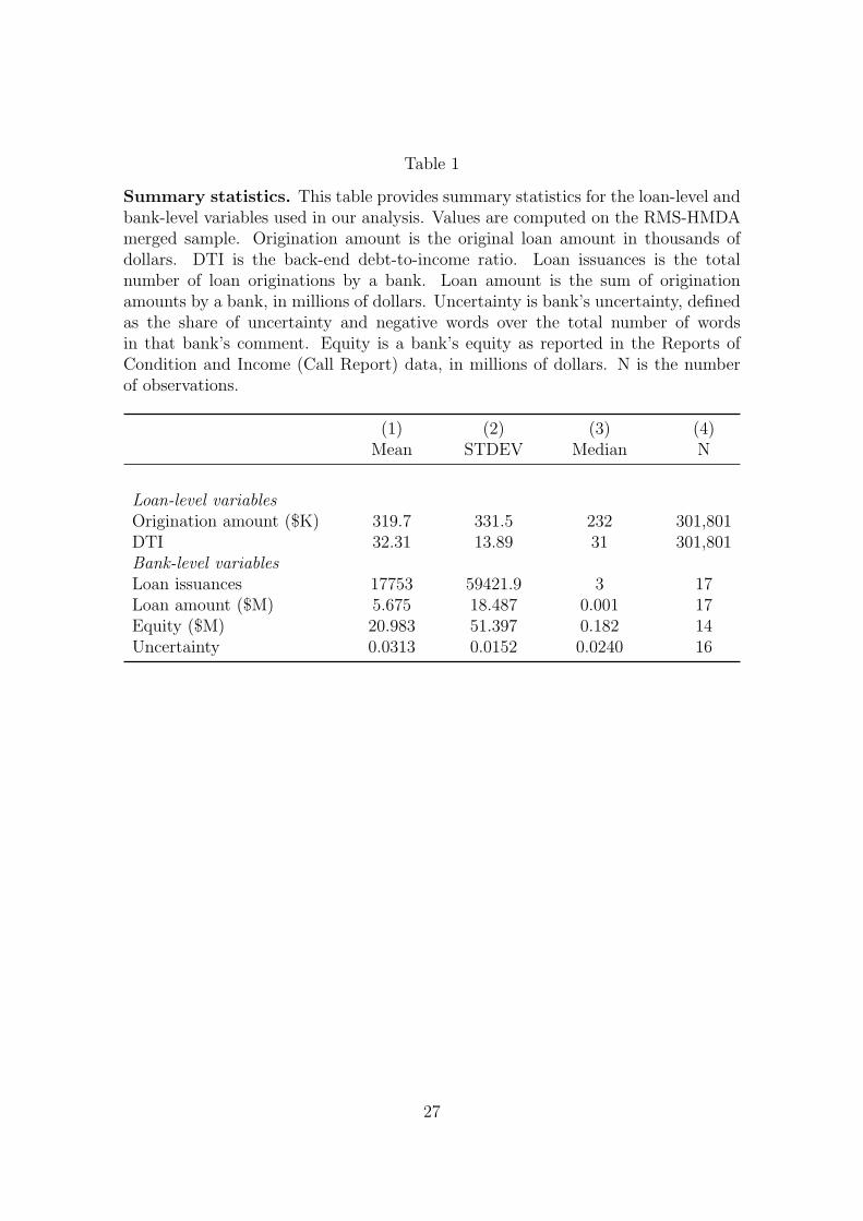
Table 1

Summary statistics. This table provides summary statistics for the loan-level andbank-level variables used in our analysis. Values are computed on the RMS-HMDAmerged sample. Origination amount is the original loan amount in thousands ofdollars. DTI is the back-end debt-to-income ratio. Loan issuances is the totalnumber of loan originations by a bank. Loan amount is the sum of originationamounts by a bank, in millions of dollars. Uncertainty is bank’s uncertainty, definedas the share of uncertainty and negative words over the total number of wordsin that bank’s comment. Equity is a bank’s equity as reported in the Reports ofCondition and Income (Call Report) data, in millions of dollars. N is the numberof observations.

(1) (2) (3) (4)Mean STDEV Median N

Loan-level variablesOrigination amount ($K) 319.7 331.5 232 301,801DTI 32.31 13.89 31 301,801Bank-level variablesLoan issuances 17753 59421.9 3 17Loan amount ($M) 5.675 18.487 0.001 17Equity ($M) 20.983 51.397 0.182 14Uncertainty 0.0313 0.0152 0.0240 16

27

Table 2

Composition of mortgage portfolio. This table provides the results of theregression: yi,t = β ∗ (proposalt ∗ uncertaintyi) + γxi,t + ϵi,t. proposalt is adummy that takes value 1 between May 2011 and December 2012 and 0 otherwise.uncertaintyi is the share of uncertainty and negative words over the total numberof words in bank i’s comment. xi,t includes bank-specific and time-specific fixedeffects. The dependent variable is the log of the ratio of the number of loans with aDTI between 37 and 43 over the number of loans with a DTI below 21 (columns 1and 3) or the log of the ratio of loans featuring a DTI ratio of 37 to 43 over the totalnumber of loans (columns 2 and 4). The first two columns report estimates for thefull bank sample while the last two columns report estimates for the sub-sample ofbanks that submitted a comment.

(1) (2) (3) (4)37−43<21

37−43N

37−43<21

37−43N

proposal*uncertainty -6.783*** -2.027 -14.03** -5.546(-3.11) (-1.36) (-2.03) (-1.23)

time FE Yes Yes Yes Yesbank FE Yes Yes Yes Yes

N 4129 8360 225 261R2 0.568 0.638 0.457 0.567

28

Table 3

Loan amount. This table reports the results of the regression: loanamounti,t = β ∗ (proposalt ∗ uncertaintyi) + γxi,t + ϵi,t. loan amounti,t is thelogarithm of the total (dollar) loan amount originated by bank i in month t, by DTIclasses. proposalt is a dummy that takes value 1 between May 2011 and December2012 and 0 otherwise. uncertaintyi is the share of uncertainty and negative wordsover the total number of words in bank i’s comment. xi,t includes bank-specificand time-specific fixed effects. The results are reported by DTI class as follows:< 21 (column 1), 21-28 (column 2), 29-36 (column 3), 37-43 (column 4), and 44-50(column 5).

(1) (2) (3) (4) (5)< 21 21-28 29-36 37-43 44-50

proposal*uncertainty -11.95** -15.57*** -16.19*** -17.76*** -12.34**(-2.09) (-2.90) (-3.38) (-3.42) (-2.53)

time FE Yes Yes Yes Yes Yesbank FE Yes Yes Yes Yes Yes

N 7165 9051 9297 8360 6136R2 0.823 0.807 0.802 0.793 0.806

29

Table 4

Loan issuances. This table reports the results of the regression: loanissuancesi,t = β ∗ (proposalt ∗ uncertaintyi) + γxi,t + ϵi,t. loan issuancesi,t is thetotal number of loan originations by bank i in month t, by DTI classes. proposalt isa dummy that takes value 1 between May 2011 and December 2012 and 0 otherwise.uncertaintyi is the share of uncertainty and negative words over the total numberof words in bank i’s comment. xi,t includes bank-specific and time-specific fixedeffects. The results are reported by DTI class as follows: < 21 (column 1), 21-28(column 2), 29-36 (column 3), 37-43 (column 4), and 44-50 (column 5).

(1) (2) (3) (4) (5)< 21 21-28 29-36 37-43 44-50

proposal*uncertainty -5375.9** -6480.3** -6420.0*** -4256.0*** -2481.4***(-2.29) (-2.49) (-2.58) (-2.62) (-2.86)


N 7165 9051 9297 8360 6136R2 0.658 0.525 0.489 0.539 0.253

30

Table 5

Loan issuances: Restricted sample. This table reports the results of theregression: loan issuancesi,t = β ∗ (proposalt ∗ uncertaintyi) + γxi,t + ϵi,t. loanissuancesi,t is the total number of loan originations by bank i in month t, by DTIclasses. proposalt is a dummy that takes value 1 between May 2011 and December2012 and 0 otherwise. uncertaintyi is the share of uncertainty and negative wordsover the total number of words in bank i’s comment. xi,t includes bank-specificand time-specific fixed effects. The results are reported by DTI class as follows:< 21 (column 1), 21-28 (column 2), 29-36 (column 3), 37-43 (column 4), and 44-50(column 5). These estimates are generated from the sub-sample of banks thatsubmitted a comment.

(1) (2) (3) (4) (5)< 21 21-28 29-36 37-43 44-50

proposal*uncertainty -9048.8** -10727.0** -10297.0** -5399.6** -3137.4**(-2.09) (-2.32) (-2.32) (-2.01) (-2.02)


N 248 261 258 261 238R2 0.403 0.379 0.396 0.400 0.444

31

Table 6

Correlation matrix: Legal cases and lending growth. This table shows thecorrelation coefficients between the number of cases where a bank appeared asthe defendant, and that were terminated by 2004, and the banks lending growthbetween 2004 and 2006, measured two ways: by the (percentage) change in total(dollar) loan amount and by the (percentage) change in total number of loanoriginations.

cases growth in l. amount growth in l. issuances

cases 1growth in l. amount 0.000264 1growth in l. issuances -0.000143 0.873*** 1

32

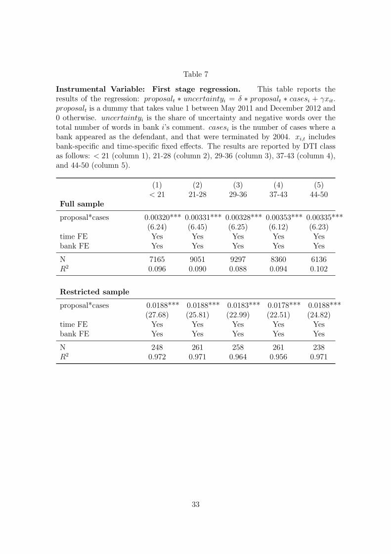
Table 7

Instrumental Variable: First stage regression. This table reports theresults of the regression: proposalt ∗ uncertaintyi = δ ∗ proposalt ∗ casesi + γxit.proposalt is a dummy that takes value 1 between May 2011 and December 2012 and0 otherwise. uncertaintyi is the share of uncertainty and negative words over thetotal number of words in bank i’s comment. casesi is the number of cases where abank appeared as the defendant, and that were terminated by 2004. xi,t includesbank-specific and time-specific fixed effects. The results are reported by DTI classas follows: < 21 (column 1), 21-28 (column 2), 29-36 (column 3), 37-43 (column 4),and 44-50 (column 5).

(1) (2) (3) (4) (5)< 21 21-28 29-36 37-43 44-50

Full sample

proposal*cases 0.00320*** 0.00331*** 0.00328*** 0.00353*** 0.00335***(6.24) (6.45) (6.25) (6.12) (6.23)


N 7165 9051 9297 8360 6136R2 0.096 0.090 0.088 0.094 0.102

Restricted sample

proposal*cases 0.0188*** 0.0188*** 0.0183*** 0.0178*** 0.0188***(27.68) (25.81) (22.99) (22.51) (24.82)


N 248 261 258 261 238R2 0.972 0.971 0.964 0.956 0.971

33

Table 8

Instrumental variable: Loan amount (second stage regression).This table provides the results of the regression: loan amountit =β ∗ (proposalt ∗ uncertaintyi)

IV + γxit + ϵit. loan amountit is logarithm ofthe total (dollar) loan amount originated by bank i in month t, by DTI classes.proposalt is a dummy that takes value 1 between May 2011 and December 2012and 0 otherwise. uncertaintyi is the share of uncertainty and negative wordsover the total number of words in bank i’s comment. The interaction term(proposalt ∗ uncertaintyi)

IV is given by the fitted values from the first stageregression summarized in Table 7. xi,t includes bank-specific and time-specific fixedeffects. The results are reported by DTI class as follows: < 21 (column 1), 21-28(column 2), 29-36 (column 3), 37-43 (column 4), and 44-50 (column 5).

(1) (2) (3) (4) (5)< 21 21-28 29-36 37-43 44-50

proposal*uncertainty -12.33 -43.45*** -36.43*** -33.48*** -21.43**(-1.22) (-4.05) (-3.91) (-3.59) (-2.46)


N 7165 9051 9297 8360 6136R2 0.084 0.071 0.065 0.062 0.042

34

Table 9

Instrumental variable: Loan issuances (second stage regression).This table provides the results of the regression: loan issuancesit =β ∗ (proposalt ∗ uncertaintyi)

IV + γxit + ϵit. loan issuancesit is the totalnumber of loan originations by bank i in month t, by DTI classes. proposalt is adummy that takes value 1 between May 2011 and December 2012 and 0 otherwise.uncertaintyi is the share of uncertainty and negative words over the total numberof words in bank i’s comment. The interaction term (proposalt ∗ uncertaintyi)IV isgiven by the fitted values from the first stage regression summarized in Table 7. xi,t

includes bank-specific and time-specific fixed effects. The results are reported byDTI class as follows: < 21 (column 1), 21-28 (column 2), 29-36 (column 3), 37-43(column 4), and 44-50 (column 5).

(1) (2) (3) (4) (5)< 21 21-28 29-36 37-43 44-50

proposal*uncertainty -11980.7***-14150.6***-13732.2***-10490.7***-10244.0***(-2.95) (-3.15) (-3.30) (-3.53) (-4.27)


N 7165 9051 9297 8360 6136R2 0.016 0.008 0.006 -0.012 -0.012

35

Table 10

Instrumental variable: Loan issuances (second stage regression, re-stricted sample). This table provides the results of the regression: loanissuancesit = β ∗ (proposalt ∗ uncertaintyi)IV + γxit + ϵit. loan issuancesit is thetotal number of loan originations by bank i in month t, by DTI classes. proposalt isa dummy that takes value 1 between May 2011 and December 2012 and 0 otherwise.uncertaintyi is the share of uncertainty and negative words over the total numberof words in bank i’s comment. The interaction term (proposalt ∗ uncertaintyi)

IV

is given by the fitted values from the first stage regression summarized in Table 7.xi,t includes bank-specific and time-specific fixed effects. The results are reportedby DTI class as follows: < 21 (column 1), 21-28 (column 2), 29-36 (column 3),37-43 (column 4), and 44-50 (column 5). These estimates are generated from thesub-sample of banks that submitted a comment.

(1) (2) (3) (4) (5)< 21 21-28 29-36 37-43 44-50

proposal*uncertainty -5733.1* -8893.3** -8613.0** -7027.8*** -2514.2**(-1.78) (-2.46) (-2.36) (-2.68) (-2.16)


N 248 261 258 261 238R2 0.283 0.258 0.273 0.259 0.280

36

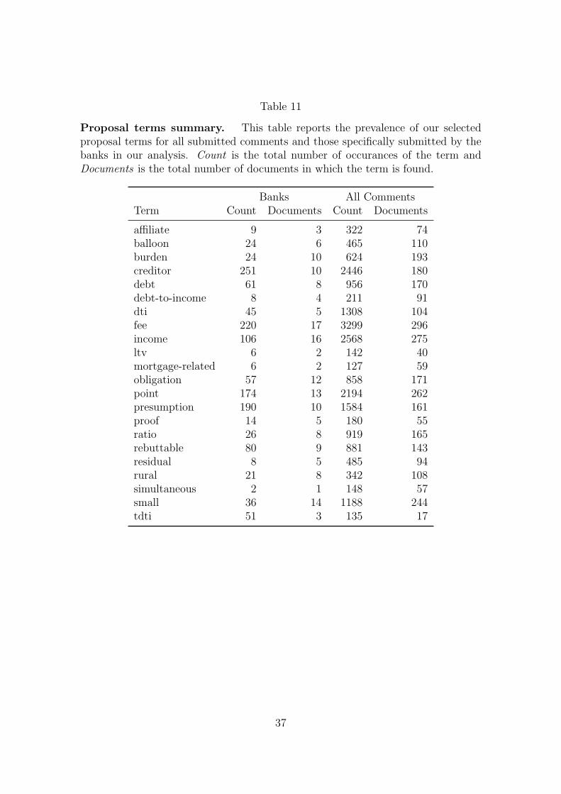
Table 11

Proposal terms summary. This table reports the prevalence of our selectedproposal terms for all submitted comments and those specifically submitted by thebanks in our analysis. Count is the total number of occurances of the term andDocuments is the total number of documents in which the term is found.

Banks All CommentsTerm Count Documents Count Documents

affiliate 9 3 322 74balloon 24 6 465 110burden 24 10 624 193creditor 251 10 2446 180debt 61 8 956 170debt-to-income 8 4 211 91dti 45 5 1308 104fee 220 17 3299 296income 106 16 2568 275ltv 6 2 142 40mortgage-related 6 2 127 59obligation 57 12 858 171point 174 13 2194 262presumption 190 10 1584 161proof 14 5 180 55ratio 26 8 919 165rebuttable 80 9 881 143residual 8 5 485 94rural 21 8 342 108simultaneous 2 1 148 57small 36 14 1188 244tdti 51 3 135 17

37

Table 12

Proposal terms ranked by similarity to uncertainty. This table ranks ourselected proposal terms by the correlation similarity measure, ρi, over the splitbetween the full corpus of comments and those submitted by banks in our analysis.

Banks All CommentsTermi ρi Termi ρi

1 proof 0.2437 proof 0.22632 presumption 0.2264 obligation 0.18723 rebuttable 0.2182 burden 0.14984 residual 0.1759 presumption 0.13885 burden 0.1664 rebuttable 0.11966 tdti 0.1594 simultaneous 0.09847 debt-to-income 0.1467 income 0.09358 income 0.1460 creditor 0.08969 obligation 0.1112 point 0.084410 simultaneous 0.0968 tdti 0.082511 ratio 0.0724 fee 0.074412 dti 0.0477 debt-to-income 0.064913 creditor 0.0465 mortgage-related 0.045214 point 0.0444 residual 0.037715 ltv 0.0443 debt 0.023816 fee 0.0365 affiliate 0.012417 mortgage-related 0.0251 ratio 0.002618 affiliate 0.0219 ltv -0.006719 debt 0.0161 dti -0.009620 balloon -0.0081 small -0.014021 rural -0.0565 balloon -0.026722 small -0.0578 rural -0.0298

38

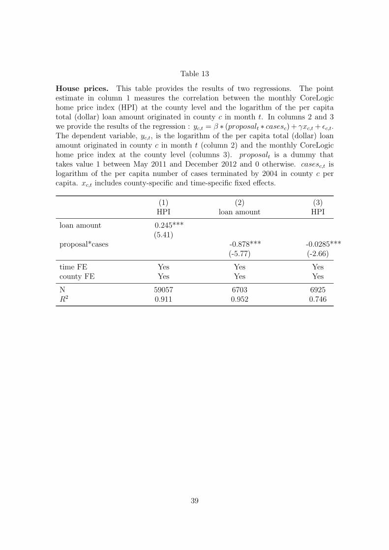
Table 13

House prices. This table provides the results of two regressions. The pointestimate in column 1 measures the correlation between the monthly CoreLogichome price index (HPI) at the county level and the logarithm of the per capitatotal (dollar) loan amount originated in county c in month t. In columns 2 and 3we provide the results of the regression : yc,t = β ∗ (proposalt ∗ casesc) + γxc,t + ϵc,t.The dependent variable, yc,t, is the logarithm of the per capita total (dollar) loanamount originated in county c in month t (column 2) and the monthly CoreLogichome price index at the county level (columns 3). proposalt is a dummy thattakes value 1 between May 2011 and December 2012 and 0 otherwise. casesc,t islogarithm of the per capita number of cases terminated by 2004 in county c percapita. xc,t includes county-specific and time-specific fixed effects.

(1) (2) (3)HPI loan amount HPI

loan amount 0.245***(5.41)

proposal*cases -0.878*** -0.0285***(-5.77) (-2.66)

time FE Yes Yes Yescounty FE Yes Yes Yes

N 59057 6703 6925R2 0.911 0.952 0.746

39

Figure 1

Loan issuances for selected DTI ratios. This graph shows the ratio of loansissued in month t and featuring a DTI ratio of 21 or less over the total number ofloans issued in t. It also depicts the ratio of loans issued in month t and featuringa DTI ratio of 37 to 43 over the total number of loans issued in t.

Rule Proposal

May 11, 2011

Final Rule

Jan 10, 2013

0.15

0.20

0.25

0.30

2011 2012 2013 2014 2015

Por

tfolio

Sha

re

DTI Class

<21

37−43

40

Figure 2

Origination amounts by DTI ratio. This graph shows monthly originationamounts disaggregated by DTI classes.

Rule Proposal

May 11, 2011

Final Rule

Jan 10, 2013

0

2

4

6

2011 2012 2013 2014 2015

Orig

inat

ion

Am

ount

($b

n) DTI Class

<21

21−28

29−36

37−43

44−50

50−60

>60

41

Figure 3

Distribution of uncertainty by comment wave. This graph shows the variationin the share of uncertain and negative words in the public comments submittedbetween 2011 and 2013.

0.00

0.05

0.10

0.15

0.20

0.25

Wave 1 Wave 2 Wave 3Comment Wave

Term

Sha

re D

istr

ibut

ion

DictionaryNegative or Uncertain

42

Appendix: Modeling topics in comments

Our corpus—a collection of documents—for this exercise is the set of public com-

ments from which we extracted our measure of a lender’s uncertainty in Section 4.2.

After tokenizing the corpus to allow for hyphenated terms, we remove stopwords—a

set of the most prevalent english words whose occurrence in a document is uninformative—

as provided by Python’s NLTK module (Bird, Klein, and Loper 2009) and then

lemmatize this set of terms so that only the dictionary forms of words appear in our

corpus vocabulary. We also filter the vocabulary to include only terms that occur

five or more times within the corpus. Our resulting corpus is composed of a dense

set of 8108 unique terms. Table 11 summarizes a subset of the corpus vocabulary

that would be the most useful for describing the proposal criteria.

Latent Semantic Similarity

Vector space models (VSMs) (Turney, Pantel, et al. 2010) extract semantic cues from

a corpus and are useful for modeling the similarity between terms and contexts (for

example, documents, paragraphs, or sentences). More concretely, latent semantic

analysis (LSA) (Deerwester, Dumais, Landauer, Furnas, and Harshman 1990, Lan-

dauer, Foltz, and Laham 1998) is a singular value decomposition on a term-document

matrix X(|V |×|D|), where |V | is the number of terms in the vocabulary V , and |D|

is the number of documents in corpus D. The decomposition X = TSD⊤ further

allows for the selection of the k most important and reliable features of the term-

document matrix and the approximation X ≈ Xk = TkSkD⊤k . The choice of k in

other applications is made with the goal of dimensionality reduction. In LSA, k is

a smoothing parameter over the sparse term-document matrix, X.

This smoothed term-document representation leads to a term-term similarity

matrix Mt = XX⊤ = TS2T⊤ and a document-document similarity matrix Md =

X⊤X = DS2D⊤ whose elements Mi,j are the dot products between columns i and

j of the term representation matrix X⊤ and the document representation matrix

43

X respectively. For high dimensional learning tasks, this reformulation provides a

tractable solution at the cost of being susceptible to variations in scale and location.

Since our task is relatively small, we instead elect to measure similarity directly

from X⊤ as the cross-correlation matrix ρ. The correlation coefficient ρi,j is more

straightforward to interpret and is equivalent to a dot product that is centered and

normalized to account for magnitude.

With this measure in mind, we would like to rank, by their similarity to our

uncertainty dictionary, the terms that pertain solely to the debt-to-income criterion

against terms that would likely correspond to other proposed criteria. We form X

using standard TF-IDF scaling (Ramos 2003) to adjust for the disparity of term

prevalence evident in table 11 and compute ρ from X40. For each criterion term

row ρi, we define the mean similarity over the 769 columns that correspond to the

uncertainty terms found in our corpus as ρi = E(ρi,j|i).

Table 12 reports ρi for each term with respect to the entire comment corpus as

well as the subset of comments submitted by the banks in our analysis. Within

the context of banks’ comments, the majority of proposal terms are more highly

correlated with the uncertainty vocabulary. The exceptions are small, creditor,

point, fee, and debt. All other terms are more closely related to uncertainty with

regard to banks’ feedback. The terms ranking highest for banks are those used to

describe the rebuttable presumption in general and followed closely by terms that

would occur in a discussion of the debt-to-income criterion. Phrases like debt burden,

residual income, debt obligation, and total debt-to-income (TDTI) ratio are used

synonymously within the public comments. Burden may also rank highly because

the phrase burden of proof is likely to co-occur in a discussion about presumed

innocence.

44

Lending on hold: Regulatory uncertainty and bank lending ...

Documents

Transcript of Lending on hold: Regulatory uncertainty and bank lending ...