DOCUMENT RESUME

ED 116 551 HE 006 928

AUTHOR Legg, K.TITLE Comparative Studies in Costs and Resource

Requirements for Universities. Technical Report.Studieskin Institutional Management in HigherEducation.

INSTITUTION Organisation for Economic Cooperation andDevelopment, Paris (France). Centre for EducationalResearch and Innovation.

PUB DATE 31 Oct 71NOTE 146p.; Paper presented at the Evaluation Conference

on Institutional Management in Higher Education(Paris, France, October, 1971)

EbRS PRICE MF-$0.76 HC-$6.97 Plus PostageDESCRIPTORS *Comparative Education; *Cost Effectiveness; *Data

Bases; Educational Planning; Expenditures; *HigherEducation; Management Develo ent; *MathematicalModels; Resource Allocations; ff Utilization;Surveys; Universities

This comparative study is' broadly divided into twoparts. The first presents a simple approximate internationallydata-based university overall mathematical resource model derivedfrom an original analysis of a 15-university international samplefrom the CERI (Center for Educational Research and Innovation)1968/1969 Information Survey. It provides a method of estimation ofstaff and costs at departmental (or equivalent structure) level interms of twelve broad subject areas and these are then used to derivestaff, areas, recurrent and sdme capital expenditures at the overalluniversity level. The results of a typical example are given. Thesecond part presents a generalized conceptual/data-based methodologyfor the calculation of university departmental academic, supportingand administrative staff by broad subject area and geographicalregion. The methodology has been specifically formulated toaccommodate different types of student programmes and the method isillustrated by example to a tipical British University. Included arerelevant observations on international university comparative dataderived from the CERI survey, (Author)

ABSTRACT

*****************************\******************************************* Documents acquired by EIC include many informal unpublished *

* materials not available from other sources. ERIC makes every effort ** to obtain the best copy available. Nevertheless, items of marginal *

* reproducibility are often'enoountered and this affects the quality *

* of the microfiche and hardcopy reproductions ERIC makes available *

* via the ERIC Document Reproduction Service (EDRS). EDRS is not *

* responsible for the quality of the original document. Reproductions ** supplied by EDRS are the best that can be made from the original. *

***********************************************************************

A,

4)

I

centre1 I for

educationalresearch

and

innovation

OECD

STUDIES IN INSTITUTIONAL MANAGEMENTIN HIGHER EDUCATION

CENTRE FOR EDUCATIONAL RESEARCHAND. INNOVATION

COMPARATIVE STUDIESIN COSTSAND RESOURCEREQUIREMENTSFOR UNIVERSITIEStechnical report

U.S DEPARTMENT OF HEALTHEDUCATION & WELF ARENATIONAL INSTITUTE OF

EDUCATIONTHIS DOCUMENT

HAS BEEN PE PRO

OUCEO EXACTLY AS RECEyED FROM

THE PERSON OR ORGANIZATIONATING iT POINTS Of

ViEA ON OP NON',

STATED DO NOT NITFSSAH t Y RF PPE

SENTO; F lC,A1 NATIONAiEDUCATION PO,,ITICIN

OR PO, 't Y

ORGANISATION FOR ECONOMIC CO-OPERATION AND DEVELOPMENT

ORGANISATION FOR ECONOMIC Paris, 31st October, 1971

CO-OPERATION AND DEVELOPMENT

Centre for Educational Researchand Innovation

cERI/Im/71.39

EVALUATION CONFERENCE ON INSTITUTIONAL

MANAGEMENT IN HIGHER EDUCATION

(2nd-5th November, 1971)

COMPARATIVE STUDIES IN COSTS AND RESOURCE

REQUIREMENTS FOR UNIVERSITIES

by

ProfessOr K. Legg,Head of Department of TranspOrt Technology,University of Loughborough, United Kingdom,

(Note by the Secretariat)

Or. engl.

This report was prepared by Professor Keith Legg as a consultant to the

Centre during January - July 1971. It constitutes one of the in-house research

activities carried out as part of the Programme on Institutional Management in

Higher Education. It is based onAhe University Information Survey conducted by

the Centre with his advice. It provides a method of estimation of staff and costsat departmental (or equivalent structure) level in terms of 12 broad subject areas

and these are then used to derive staff,'areas, recurrent and some capital expendi-

tures at the overall university level. The results of a typical example are given.

The report then presents a generalized conceptual/data-based methodology for

the calculation of university departmental academic, supporting and administrative

staff by broad subject area and geographical region. The methodology has beenspecifically formulated to accommodate different types of student programmes andthe method is illustrated by example to a typical British university.

(.3

COMPARATIVE STUDIES IN COSTS AND RESOURCE

REQUIREMENTS FOR UNIVERSITIES

This report has been prepared by Professor Keith Legg, Head of the

Department of Transport Technology, The University of Technology, Lourhhorough,

England, and Consultant to CERI.

The paperis broadly divided into two parts. The first presents a simple

approximate internationally data-based university overall mathematical resource

model derived from an original,analysis of a 15-University international sample

from the CERI 1968/1969 Information Survey. It provides a method of estimation-

of staff and costs at departmental (or equivalent structure) level in terms of

12 broad subject areas and these are then used to derive staff, areas, recurrent

and some capital expenditures at the overall university level. The results of a

typical example are given.

The second part presents a generalized conceptual/data-based methodology

for the calculation of university departmental academic, supporting and adminis-

trative ataff,by broad subject area and geographical region. The methodology has

been specifically formulated to accommodate different types of student programmes

and the method is illustrated by example to a typical British University.

The paper includes relevant observations on international university

comparative data derived from the CERI survey..

CONTENTS

Page No.

CHAPTER 1. An Approach to University Planning 1

CHAP'T'ER 2.

1. The General Approach 2

2..A Simple Data - Based. Model for Overall University

Resource Requirements 4

3. A Conceptual Methodology for DepartmentalRequirements 5

A Simple Data-Based Methodology for the Determination

of University Resource Requirements 9

1. Introduction 10

2. Determination of Departmental Requirements 11

3. Overall University Requirements 15

4. Parameter Values deduced from the International

Survey 31

5. Example Application of the Methodology' H4.0

CHAPTER 3. Conceptual Methodology for the Determination of

Departmental Requirements 47

1. Introduction 48

2. Academic Staff Eatimition 48

3. Estimation of Departmental Technical SupportStaff 70

4. Estimation of Departmental AdministrativeStaff 74

Appendix Al 79

Appendix A2 81

CHAPTER 4. Comparative Data Analysis

1. Introduction

2. A Brief 15-University Sample Approximate Data

Comparison

3. Further Data Observations on a larger International

Survey

Appendix A3

(1)

LIST OF TABLES

Page No.

Table I. Values of Departmental Parameters - 15-UniversitySample 32-33

Table 2. Overall University Primary Constants - 15- University' Sample 34-35

Table 3. Overall University Secondary Constants 15-Universi4,Sample ' 36

Table 4. Departmental Constants Classified by Region andSubject Area - 80- University Survey : 37

Table 5. Overall University Primary Constants - 80- UniversitySurvey 38

Table 6. Overall University Secondary Constants - 80- UniversitySurvey

Table 7.

Table 8.

39

Departmental Student Data Example 40

Departmental Calculations - University "X" and AverageUniversity

Table 9. Overall University "X" Requirements

Table 10.

4].

42-44

A Selected Summary of Results - University "X" andAverage University 45'

Table 11 Programme of Study Distribution Factors 55

Table 12. Parametric Data for Subject Classification 62

Table 13. geographical Region Weighting Factors 62

Table 14. Programme Distribution Factors: Example 67

Table 15. Programme Distribution Factors: Example 68

Table 16. Total F.T.E. Academic Staff Requirement - TransportDepartment EXaMple 70

Table 17. Values of proportions d1, d2, d3, d 72l' 2' 3' 4.

Table lb-. Data-Derived Values of w and r . 73

Table 19. Proportions of Administrative and Technical Staff to-Academic Staff, by Department 76

Table 20. Weighting of Fundamental/Advanced Level Students 81

Table 21. Ratio of Supporting Staffs Academic Staff 82

b

LIST OF TAPITRS (Continued)

Page No. -

/Wale 22. Values of Support Area/Student' 88

Table 23. Values of r by Subject Fields 89

Table 24. Comparison ofDerived Values of t 90

Table ,25. Seletted Data.for Single Departments in SpecificUniversities and Corresponding Parameters Analysed

Table 26. Subject Field Department Classification

Table 27. Selected Overall University Ratios Classified by SubjectArea

Table 28. Selected Departmental Ratios by Subject and Geographical

Region

Table 29. Selected Departmental Ratios, Aggregated Averages, by'

Subject

Table 30. Selected Departmental Data - Overall Averages

Table 31. Method of Subject Classification Cost Ranking

Table 32. Ratio parameters for Subject Classifications byGeographical Groupings.

Table 33. Salary Ratings for all Staff Categories

Table 34. Ratios of Staff Numbers, by Type of Staff

Table 35. The Distribution of Students to Academic Staff

Table 36. Building, Recreation and Car Park Areas as % of

"Used" Land

Table 37. Unit Gross Areas Relating to Land and Building

Table 38. Building Floor Area Ratios

Table 39. Net Floor Unit. Ratios

Table 40. Recurrent Expenditure Ratios and Distribution

Table 41. Annual Average University Capital Expenditures

Table 42. Ratio Distribution of Average Annual Capital Expenditures

Table 43. Annual Building Capital Growth -'Approximate Averages

Table 44. Comparative Capital and Recurrent Expenditure Data

7

LIST OF TABLES (Continued)

Table 45. Standardized Comparative Recurrent and Capital Expendituresper Staff Member

Table 46. Conversion Exchange Rates and Approximate Cost Indices forInternatiOnal Comparison

Table 47. Overall University Data

Table 48. Faculty Data - 80-University Survey

Table 49.

Table .50.

Table 514

Table 52.

Values of Departmental Teaching Parameters, by SubjectArea

Values for Average Staff Teaching Loads per Week

Subject Classification Parameter Values

Aggregated Departmental Data by Subject Clagsificationfor all Sample Universities

Page No.

CHAPTER 1. AN APPROACH TO UNIVERSITY PLANNING

1.-The General Approach

2. A Simple Data -Based Model for Overall University Resource

Requirements

3. A Conceptual Methodology for Departmental Requirements

Page No.

2,

5

1. The General Approach

Systematic evaluation of the university function has been a much-neglectedsubject. Universities have become so :closely associated with the term "academicfreedom" that attempts to formalise their function have invariably been resisted onthe basis of violation of this ancient heritage. SUch resistance can, however,be justified quite easily on the grounds of the complexity of the problem involvingas it does the human equation of young people during their most intellectuallyformative years. However, the need for and rapid growth of higher educationdemands the application of the most sophisticated management principles to theorganization and running of universities if the present confusion is not todegenerate into chaos. Thus in recent years there has been a grc h in researchactivity_ in this area with particular emphasis on a systems approach. Themajority. of work has concentrated on descriptive model techniques which, although

I probably more acceptable to the average academic, limit the degree of comparativeanalysis_ that can be made and tend to be of a localized 'nature. Formulae areregarded with suspicion and, if not firmly controlled, can lead to complicateddetail and rigid application. Nevertheless, the analytical approach providesconsiderable flexibility, particularly for a generalized overall system, and ifused within its limitations can provide broad guidelines whilst obviating theprinciple that "whoever shoUts loudest gets most!".

With these considerations in view a simple mathematical approach toacademic plaraLing was developed at the University of Loughborough, and has becomeaccepted as a'good management aid for those aspects of staff and space on whichit concentrates. Principally it serves as a guide for equitable provision acrossthe university for existing co tments and the determination of- future requirementsconforming to University policy.

Arising'out of this early work at Loughborough, OERI/OECD conducted aninternational survey of 80-Unive sities in 1970/1971, with an objective of providinga data basis for further analytical investigation. From the total survey, 15-universities submitting the most complete returns were selected for more intensiveanalysis. The methods of data processing are detailed in reference 6.

Analysis of the 15-university sample is the basis for the simple overalluniversity model. This data facilitated the evaluation of relationships betweenstudent enrolment, staff and space requirements,, and recurrent and capital'expenditure. Although the final model stands independent of the data andlyris, itsapplication depends upon knowledge of the model constants. One source of thisknowledge is the survey.

In addition to the initial data-based model, a more conceptual model isdeveloped at the departMental level. Both the overall model and the departmentalmodel are based on definitions of the academic staff function related to teaching.Though resea-fbh,and other duties of academic staff are not explicitly included,the selection of teaching can be justified on the grounds that it is the "raisond'Otre" of the university. In any case, the use of an average teaching loadparameter takes into account, implicitly, time devoted to these other activities.

The extended data-based methodology of the overall university model canassist in a wide range of problems, between as well as within, universities.

Applied to individual institutions, using their own initial data, it would beuseful in. simple planning, forcasting and resource allocation between departments,and at university level. Applied nationally or internationally it facilitatescomparative inter-institutional studies of the different resource elements, forthe planning of resource needs for new institutions and,growth of existing ones.

_LU'

Specific approximate individual studieS e.g. comparative approximate costs per

student in broad subject areas could be aided, at. any of these levels, by

application of the methodology.

The second, more conceptual framework for determining departmental

requirements enables a more exact assessment of absolute levels of resource

needs. Modification to make it operative as a sub-model for the overall

university model is possible.

2. A Simple Data -R ed, Model for Overall University Resource Allocation

This overall university model develops a series of relationships, expressed

algebraically, between the component elements of the university. Its essential

purpose is to aid in resource allocation within and between universities. With

this in mind values of paratheters, necessary for model solutions, are provided

from the university survey.

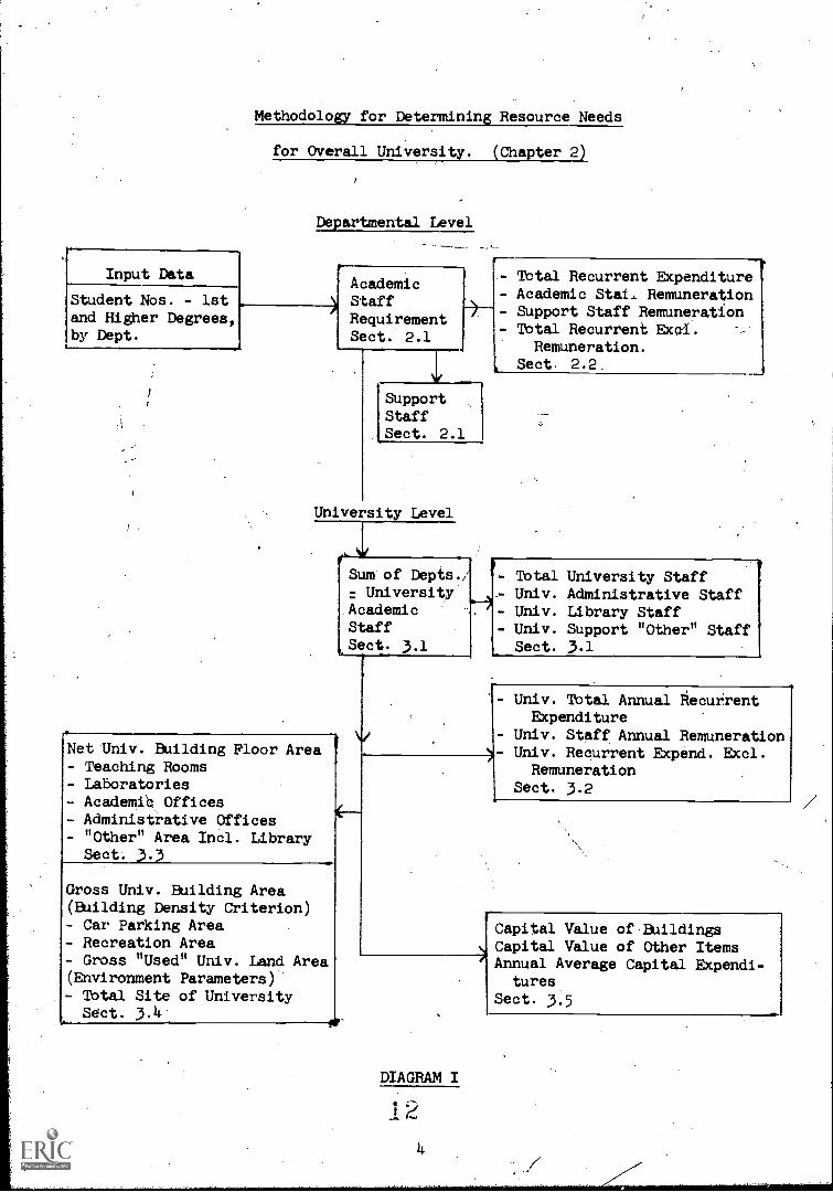
A simple explanation of the methodology is set out in diagram I (section

numbers refer to appropriate points in the model Chapter 2). It commences at

the departmental-level where input data on student enrolment, classified into

1st degree and higher degree, is required. Each department is classified into

one of ten broad subject areas. At this point academic staff requirements for

each department can be define di. Academid staff: numbers determine supporting

staff requirements (technical, administrative etc.), and annual recurrent expendi-

ture at the departmental level.

TO procede from this stage to the Overall university it is necessary to

make several assumptions. The simplest set, utilized here, is that all students

and academic staff are attached to a particular department. In a specific

context different assumptions re the relationship of departthental students And

staff and overall university numbers may be more appropriate. These can be

incorporated without undue difficulty under the present assumption the sum of

departmental students and academic staff equal the corresponding university

figures.

Relationships can now be\developed at the university level. Administrative,

library, technical and other staff are expressed in terms of total academic staff.

Simple algebraic substitutions enable university' annual recurrent expenditure,

and its components, to be expressed similarly.

University space requirements are categorized into various groups according

to function. These are, broadly, net university building floor area, gross

university building area, recreational facilities, and car parks. The first

category is further subdivided into teaching rooms, laboratories, academic and

administrative staff offices, library and "other" areas. Each of these components

is evaluated independently, and all are reducable to expressions in which academic

staff is the only independent factor.

University used land area is the sum of gross building area, recreational

and car park areas. In order to assess the total site requirement from this,

building density ind'environmental desirability' factors are introduced.

To convert ese capital requirements into monetary terms, it is necessary

to know the cost p r square unit of the different types of provisions. If growth

is envisaged, the ercentage growth rate of the student populated must.

Input Data

Student Nos. - 1stand Higher Degreesby Dept.

Methodology for Determining Resource Needs

for Overall University. (Chapter 2)

Departmental Level

AcademicStaffRequirementSect. 2.1

SupportStaffSect. 2.1

University Level

Net-Univ. Banding Floor Area- Teaching Rooms- Laboratories- AcademiC Offices- Administrative Offices- "Other" Area Incl. LibrarySect 3.3

Gross Univ. Building Area(Building Density Criterion)- Car Parking Area- Recreation Area- Gross "Used" Univ. Land Area(Environment Parameters)- Total Site of UniversitySect. 3.1

rly

Sum of Depts./University

AcademicStaffSect. 3.1

Total Recurrent Expenditure- Academic Ste. Remuneration- Support Staff Remuneration- Total Recurrent Excl.. -

Remuneration.Sect. 2.2.

4

1.7)

DIAGRAM I

12

Total University StaffUniv. Administrative StaffUniv. Library StaffUniv. Support "Other" StaffSect. 3.1

Univ. Total Annual RecurrentExpenditure

Univ. Staff Annual RemunerationUniv. Recurrent EXpend. Excl.

RemunerationSect. 3.2

Capital Value of BuildingsCapital Value of Other ItemsAnnual Average Capital Expendi-

turesSect. 3.5

1\

The crucial element in the practical application of this methodology is a

knowledge of the parameter values with the algebraic functions. Approximate

values for these parameters were obtained from 15-university sample, and from the

80-university OECD survey. These values are presented in section 4 of Chapter 2.

Due to the quantity of data a computer programme calculating these constants was

written. The results of the 15-university sample are cross-tabulated by three

regions - North America, United Kingdom and Europe, and by the ten broad subject

arcas,divised'., An overall average situation across all regions was also

as a basis for general comparison. These could be used as approxi-

mations in determining requirements of departments, by university personnel, and

of universities, by natic-u1 :bodies. Approximations drawn from the large 80-

university survey, classified into five regions plus an overall average, are also

presented.

Alternatively a university or national body could collect data to develop

parameter values more closely related to their own context. The decision to

do this would rest on whether the accuracy obtained merited the additional

'Work involved. This would almoWcertainly require computer facilities, although

the programme available at CERI could be of assistance. It would also necessitate

that universities look closely at their own management data services. In this

paper, methodology is emphasized rather than the accuracy of detail.

One further feature of the model is that, although it is built up logically

step-by-step, functions enabling the calculation of particular requirements of immedi-

ate interest, can be extracted, without necessitating a great deal of computation at

earlier stages.

3. A'Conceptual Methodology for Departmental Requirements

An alternative, more-conceptualized departmental model which analyses the

complex functions of a department as an entity, has been developed. This provides

a complete methodology for determining departmentallresource needs whereothe

department is responsible for a whole range of different courses of study, where

its staff teach in other departments, and where it turn benefits from staff

external to the department.

The bEsis of this methodology is the generalized "programme of study"

concept. A "programme of study" is those requirements which must be satisfied in

o er to qualify for a degree or diploma. From this concept is derived a general

eq ation applicable to any course of study run by a department. This might be an

and graduate degree course, post-diploma research studies, short courses, etc. The

depa tments student enrolment is classified into three groups - fundamental, advanced

and higher.

From these categories it is possible to compare different programmes of

study from different educatidhal systems far more directly than with the simpler

1st degree/higher degree classification of the overall model. Each department

can categorite its programmes of study more finely, and weightings of requirements

for different levels of students can be more exact.

A programme of study under the auspices of one department, y e taught by

academics attached to both-that department and other departments. This service -

teaching between departments ii'explicitlyincorporated in the alysis by means of

distribution factors. Thus the contribution by academic staff of any particulardepartment to various programmes of study irk accounted for in determing the

departmental staff needs.

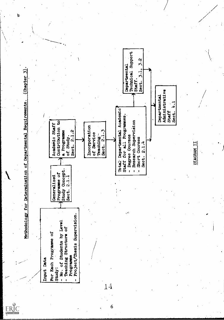
Methodolo

for Determination of De artmental Re uirements.

Chaster 3

Input Data

Fbr Each Programme of

Study:

- No. of Students by Level

- Teaching Structure of

Programme

- Project/Thesis Supervision.

Generalized

Programme of

Study Concept.

Sect. 2.1.1

Acadelilic Staff

Contribution-to

a Programme

of. Study.

Sect. 2.1.2

Incorporation

of Service

Teaching -

Sect. 2.1.3

TOW: Departmental Academic'

Staff' for all Programmes.

- Degree Courses

- Research Supervision

- Short Courses

Sect. 2.1.4

DIAGRAM II

)

Departmental

Technical Support

Staff.

Sect. 3.1, 3.2

4e

Departmental

Administrative

Staff

Sect. 4.1

Given the data on different levels of students, and the detailed structure

of teaching of each, programme of study, it is hence possible to obtain a more

accurate assessment of the absolute academic staff requirements of any particular

department. In addition a means of assessing the composition of this in terms

of part-time and full-time staff is included.

Technical and other support staff (excluding administration) is postulated

as a function of departmental support area, including laboratories and other

,working space neceslisry for the adequate functionning of the department,, Although

(technical support stiff is also related to academic staff, data from the 80-

'university survey suggests that this relationship is small. The method also

enables, as a by-product, the assessment'of departmental support area requirements.

Departmental administrative staff is related to total departmental academic

and technical staff. Furthermore it is a reasonable assumption that the -degree

of administrative servicing is related to the level of responsibility of these

other staff. Hence administrative staff are a function of departmental staff,

weighted for differing levels of responsibility.

The framework of this mire- conceptual departmental model is illustrated in

Diagram II. Section numbers are included to facilitate reference to the detailed

exposition in Chapter 3.

In addition to the two models, a good deal of data interpretation is

included throughout, especially in Chapter 4. As well as providing insight for

analytical investigation for the models, this information is useful in its own

right.

The application of such management aids as these models would dearly be much

simpler with completer facilities, due to the large quantity of data and calculation

involved. In any case the compilation of such' information is required for effective

running of a university. Although it is an administrative task to set up the

process, it is essential to involve academic staff at all levels and at all stage.

This is paiticularly important in assessing the inputs of data.

The total methodology serves as an aid in the decision-making process, by

providing information and assessment of resource needs. It is not a substitute

for the policy making process itself.

4

7

CHAPTER 2. A SIMPLE DATA-BASED METHODOLOGY FOR THE DETERMINATION

OF UNIVERSITY' RESOURCE REQUIREMENTS.

Page No.

1. Introduction 10

2. Determination of Departmental Requirements 11

2.1. Staff

2.2. Annual Recurrent Expenditure

3. Overall University Requirements

12

13

3.1. Staff 16

3.2. Annual Recurrent Expenditure 18

3.3. Net University Floor Area 23

3.4. Gross University Site Area 25

3.5. Total Capitalzand Annual Capital Expenditure 28

.Parameter Values deduced from the International Data 31

5. Example Application of the Methodology 40

i i;

9

\!

1. Introduction

The-methodology for the determination of university resource requirementsdeveloped in this chapter is a set of simple data -based relationships. Analysisof the 15-university survey data revealed certain parameter values linkingdifferent variables (see Chapter 4, sections 2.2, 2.3 and 2.4). This allowed afirst approximation of how the variables relate to one another.

In contrast to the more conceptual departmental model of Chapter 3, thismethodology has potential utilization at the university, national and internationallevels. It does not allow an absolute value assessment of requirements ofindividual departments, but provides approximations for comparative purposes.However, with some further development the methodology of the mor conceptualdepartmental model could be utilized as input data, for absolute assessments ofdepartments, within the overall university model. This would then replace thegeneral departmental section 2 of the present chapter.

The model presented here, together with the sets of parameter values whichcould be utilized in practical evaluations, could assist in the following problems

(i) Application to individual institutions, using their own initial data,for simple planning, foredasting and resource allocation.

(ii) Comparative inter-institutional or international studies.

(iii) Approximate resource needs for new institutions and growth needsfor existing ones.

(iv) Specific individual studies e.g. comparative approximate costs perstudent in broad subject areas.

The complete model commences at the departmental and proceeds to theoverall university. At the forme level, each department is classified into the10 broad subject classification areas' of Chapter, 4, table 2. Input data on thenumber of first degree and "all higher" degree students in,a department (associatedwith the 15-uniVersity questionnaire) enables the evaluation of staff weeklyteaching hours and academic, support and total departmental staff. This can thenbe translated into annual recurrent expenditure.

After the determination of these resources peculiar to a department, overalluniversity relationships are developed. Academic staff for the university is thesum of departmental.needs. Administrative, library and "other" staff (e.g.technicians etc.) totals are related directly to academic staff. The functionslinking annual remuneration recurrent expenditures on these items to numbersrequired are outlined. Tb this is added recurrent non-staff expenditure, to givetotal annual recurrent expenditure for the university. On the assumptionsutilized here, this equals the sum of departmental recurrent expenditures andcentralized service expenditure (library, adMinistrationetc.).

Net university floor area is the sum of area requirements for teaching rooms,.laboratories, staff offices, both academic and administrative, library and "other".Each of these-is related in turn to academic staff, determined previously. Bycontrast, gross building area is related directly to academic staff in a proportionateway, and will always be greater than net floor area'described above. Gross buildingarea, together with car parking and recreatici facilities yields total usable site.With the introduction of site density and llehlrlronmental limiting" factors, this istranslated into total university site.

The total capital of a university is the monetary value assigned to its stockof buildings and other equipment: A simple costing procedure is outlined. AnnUal

1 (10

average capital expenditure presumes a growth situation, based on growing student

population, and its evaluation in relation to academic staff can prove a useful

guide for estimating expansion costs.

In order to demonstrate the usefulness of the procedure as a complete entity,

two possible sets of parameter values, based on the 15-university and 80-universitysamples respectively, together with a complete example, are presented in parts 4 and

5. However the model can provide information on specific items of university reqUire-

ments relatively directly without necessitating a full evaluation of relevant para-

meters. Hence academic staff for a department, for example, could be investigatedusing only the relevant sections.

At many points in the methodology, alternative evaluations of parameters are

detailed.- This is done to obtain the rout accurate assessment of parameters rela-

ting the variables. In general the simplest means is presented first, followed by

the more complicated.

2. Determination of Departmental Requirements

Each department is classified by broad subject field i, as shown in table 2

of Chapter 4. Student population is subdivided into first degree and "all higher"

degree levels, as in the university questionnaire. This contrasts with the threedivisions of fundamental, advanced and higher students utilized in the more concep-tual departmental model of Chapter 3 (section 2.1.1.).

Using input data on student numbers, staff weekly teaching hours, and hence

academic staff numbers, are determined. Flowing from this point are relationships

rot "other" departmental statf (technicians, administrative, etc.).

\ Let FT - total departmental studentsTi

FU = total departmental students - all first degrees

F0

= total departmental students - all "higher" degrees,

where 1 denotes the ith,broad subject group (1 LI 1, 2, 10).

Let FT

- (F0 + FG)ii

and total student population across all departments, F, is:

1

Tiz (FU + FG)i

Total undergraduate student population, all departments,

iFi ,

1

Total "higher" degree students in all departments,

iF6 = F61

Definitions. These relationships derived from the 15-university sample.Values for the ratios are given in table 4 of Chapter 4, together with the data

analysis.

Let A be the ratio of departmental academic staff (DA) ) to total departmental

staff (DT)DA

A =

T

Let B be departmental weekly total staff teaching hours (TT per academic

staff member (DA).

.B TT/DA

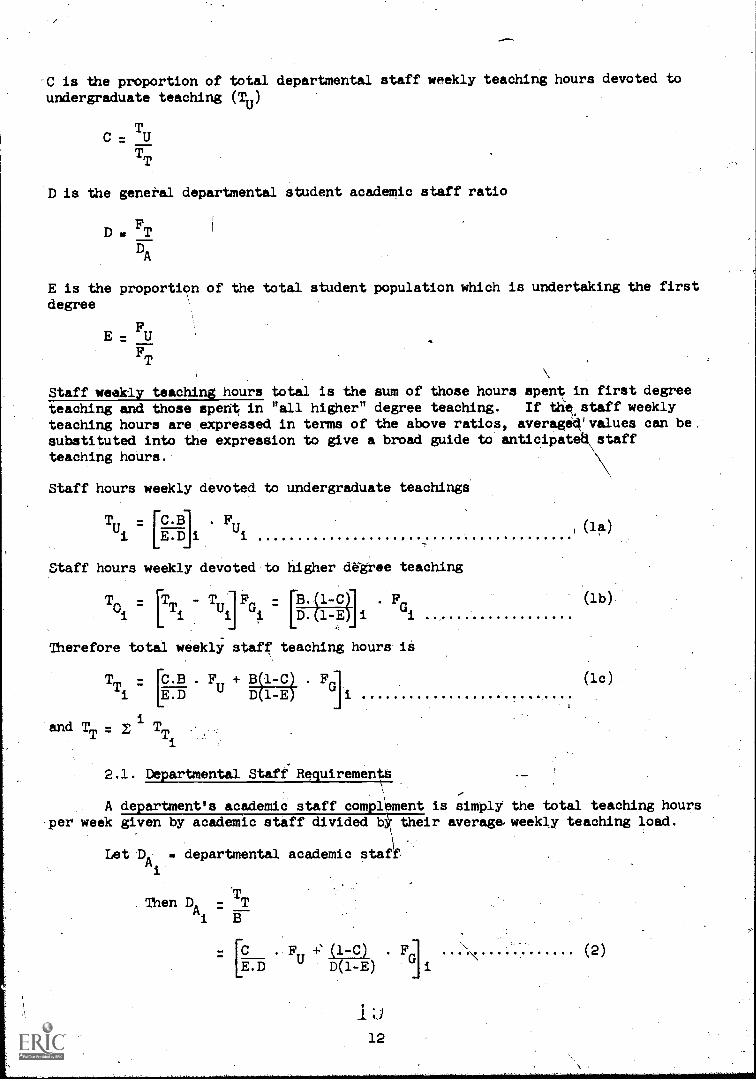
-C is the proportion of total departmental staff weekly teaching hours devoted toundergraduate teaching (Tu)

C UTT

D is the general departmental student academic staff ratio

DFT

DA

E is the proportiOn of the total student population which is undertaking the firstdegree

E = FUFT

Staff weekly teaching hours total is the sum of those hours spent in first degree

teaching and those sperit in "all higher" degree teaching. If tlkstaff weeklyteaching hours are expressed in terms of the above ratios, averag lues can be.

substituted into the expression to give a broad guide to staff

teaching hoUrs.

Staff hours weekly devoted to undergraduate teachings

Tu

[C.E] F, (la)

E.D i

staff hours weekly devoted to higher degree teaching

T - ['r. - Tu ]Fri .7 [B. ..1- 1 . F,0 T

I, i i `'i p. 1-E) iui

(lb).

Therefore total weekly staff teaching hours is

TT =

r .B . F (1c)U

D 1-Ei E.D+ B(1-1 . F ]

Gi

'andi

Z TTT _Ti

2.1. Departmental Staff RequirementS

A department's academic staff compliment is simply the total teaching hoursper week given by academic staff divided be their average weekly teaching load.

Let-DA

. departmental academic staf

. Then D. - TB

[C . F -t= (1-C) . FE.D U D(1-E) "

12

(2)

and DA - z DA Ai

*here DA

is the total academic staff attached to all departments in a university,

academic staff is in direct'proportiOn to total departmental staff such that:

[DA] A,F

or DT [DA]

i A

and DT z

(3)

"Other" departmental staff is the difference between total departmentalstaff and academic staff

If D0

- "other" departmental staff

D0

- DT

- DA

= Do = DT - DA

Given that values of A, B, C, D and E are available by subject and byregion, as an example, table 1 of section 4; the departmental staff requirements arenow defined.

2.2. Annual Departmental Recurrent Expenditure

This is in effect the assigning of an annual monetary value to staffresources and other items.

Let VT - total departmental annual recurrent expenditureTi

total departmental, staff

F = average annual recurrent expenditure per staff member.

FVT

'T

(for the derivation of the value of F, see 2.1.2. and.2.1.3. of Chapter 4).

Therefore total departmental annual recurrent expenditure is the product ofaverage expenditure per staff member and the departmental staff complement.

=[F.9

2 u13

from (3), . F . DA

A(5)

Analysis of survey data.provides average values for F and A by region andsubject area (see sections 2.1.2. and 2.1.3. of Chapter 4). Hence VT is directlycalculable from academic staff.

Departmental recurrent expenditure can be subdivided into that devoted toremuneration of academic and support staff and that devoted to other items.

Total departmental staff'annual remuneration is the product of the averageremuneration petstaff member and the total number of staff.

Let V - departmental total staff remuneration per-annuMNi

average annual remuneration per staff member.

i.e. e = VN

VT

Then

V [6.- 1Ni

from (5), .7..[F.6 . DA

A

and VN

(6)

This total remuneration expenditure per annum is made up of that devotedto academic staff and that devoted to other support staff.

Then

Let VA

- total departmental academic staff annual remuneration

H = average annual remuneration per academic staff.

i.e. V'- A

DA

A, =

VA

(7)

i.e. departmental academic staff annualsremuneration is the,prOduct of the averageannual remuneration per academic and the member of academic staff.

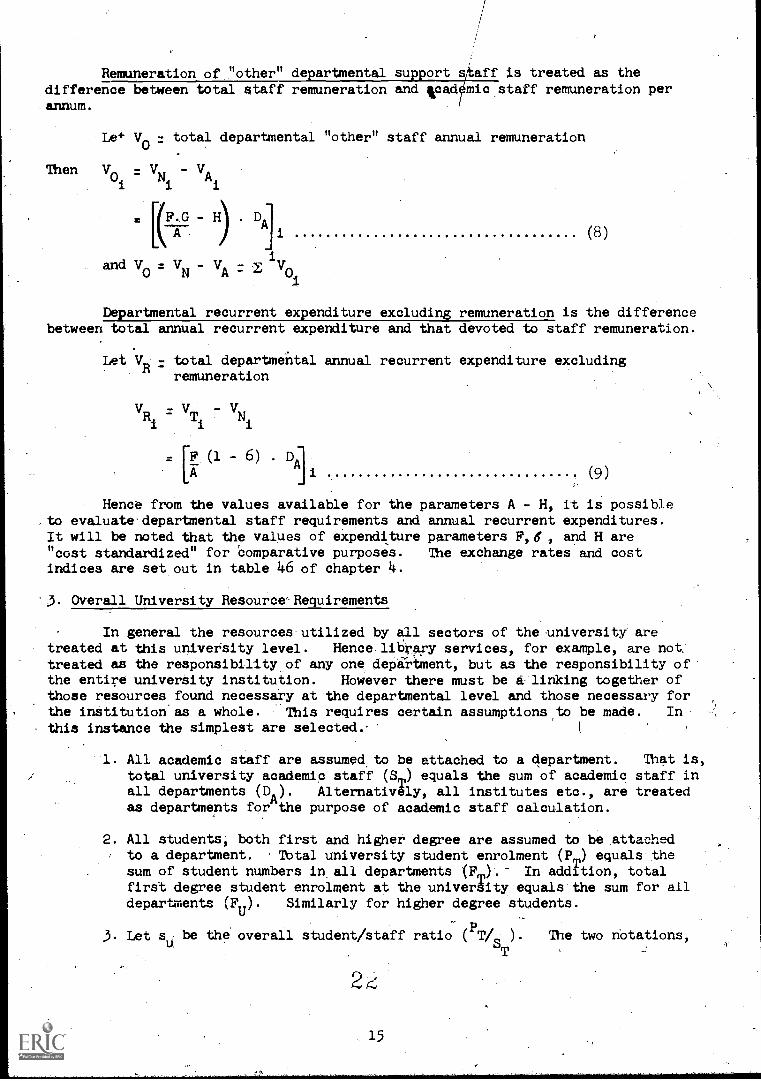
Remuneration of "other" departmental support staff is treated as thedifference between total staff remuneration and tcadmicstaff remuneration per_annum.

Le* V0

- total departmental "other" staff annual remuneration

Then V - V - V A0i

Ni i

F,G - H) .

-m

A

andV-V-V - 1N A 0

(8)

Departmental recurrent expenditure excluding remuneration is the differencebetween total annual recurrent expenditure and that devoted to staff remuneration.

Let -VR total departmental annual recurrent expenditure excludingremuneration

V - V - VRi Ti Ni

IF ( - 6) .

Am

(9).

Hence from the values available for the parameters A - H, it is possibleto evaluate. departmental staff requirements and annual recurrent expenditures.It will be noted that the values of expenditure parameters F,6., and H are"cost standardized" for comparative purposes. The exchange rates and costindices are set out in table 46 of chapter 4.

3. Overall University Resource Requirements

In general the resources utilized by all sectors of the university aretreated at this university level. Hence library services, for example, are nottreated as the responsibility_of any one depirtment, but as the responsibility ofthe entire university institution. However there must be a:linking together ofthose resources found necessary at the departmental level and those necessary forthe institution as a whole. This requires certain assumptions.to be made. Inthis instance the simplest are selected.

1. All academic staff are assumed to be attached to a department. That is,total university academic staff (Sm) equals the sum of academic staff inall departments (D ii). AlternativAly, all institutes etc., are treatedas departments for the purpose of academic staff calculation.

2. All students, both first and higher degree are assumed to be attachedto a department. Total university student enrolment (P ) equals thesum of student numbers in all departments (Fm)--- In addition, totalfirst degree student enrolment at the university equals the sum for alldepartments (FU). Similarly for higher degree students.

3. Let su. be the overall student/staff ratio (PT/S

). The two notations,

2

departmental and university, have been kept distinct as other assumptionsare clearly possible, and, may be necessary, for example, where independantinstitutes contribute importantly to teaching or student supervision.The total university notation will be employed for the remainder of themodel.

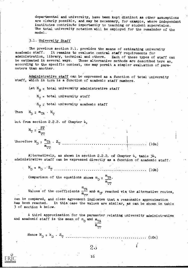
3.1. University Staff

The previous section 2.1. provides the means of estimating universityacademic staff. It remains to evaluate. central staff requirements foradministration, library, technical and others. Each of these types of staff canbe estimated in several ways. These alternative methods are described here as,according to the specific context, one may permit a simpler evaluation of para-meters than another.

Administrative staff can be expressed as a function of total universityStaff, which in turn is a function of academic staff numbers.

Then

Let ND r. total university administrative staff

total university staffNT = _

ST

total university academic staff

ND = mTA NT

but from section 2.2.2. of Chapter 4,

T mTT

Therefore ND

-mTA .

TmTT

(10a)

Alternatively, as shown in section 2.2.2, of Chapter 4, table 34,administrative staff can be expressed directly as a function of academic staff.

N - m .

D D T t ir (10b)

Comparison of the equations shows nip mTA.

mTT

Values of the coefficients --- and m reached via the alternative routes,mTA

TTEP

can be compared, and cloSe agreement indicates that a reasonable approximationhas been reached. In this case the values are similar, as can be shown in table3 of section 4 below.

A third approximation for the parameter relating university administrativeand academic staff is the mean of m

Dand m

TA

Hence ND k . SD D T

mTT

16

(1oc)

where k - i mTA + mD D1 .s---11

mTT[

Library staff can be expressed as a function of student enrolment, and henceacademic staff, or as a function of total university staff, in turn translated into

terms of academic staff.

Let 50= total university library staff

NT = total university staff

PT - total university student population

NL

- P. (see table 34, section 2.2.2. of Chapter 4).T

but PT- s

u. S

Twhere a

uis the student: staff ratio

therefore Nh su . ST

mp

Alternatively:

Nh r, mTL . NT (see table 34, section 2.2.2. of Chapter 4).

but Nm - ST

TT

therefore Nh = Th

TT

(11a)

(11b)

Hence there are again two alternative values, Bu andmTL linking library and

and academic staff. mp TT

The third approximation would again be the mean of these two alternatives:

Hence NL = . ST(11c)

[

where kh -

-

7TT

su

p

Technical and other staff canAe-expressed directly as a function ofacademic staff, of. cante treated a residual - the difference between totaluniversity staff and the sum of academic, administration and library elements.The values of constants below are shown fpom the 15-university sample,' is table 34,

Chapter 4.

`Let N0

- total university technical and other staff

ThenN0=111TO. STmTT

(12a)

Alternatively:

N _ N-S-N- N0 T T D L

but NT,

NA, Nh

are all functions of ST, as shown above. Using the

equations (10c), (lie),

SN0 c -.ST - kr) . ST kL - ST

TT

Cm- - kD

- khT.

TT(12b)

Alternatively (10a), (11a), or (10b) and (llb) substitutions could be used forN ND' L.

The third, mean, value for the parameter linking technical and academicstaff is:I

N - k . S0 0 T

wherek0

-2

+ m - kD

- k.]L

mTT

(12c)

Tbtal university staff can be expressed directly as a function of totalacademic staff, as Utilized above'.

NT

-ST

mTT (13a)

or, alternatively, as the sum of the staff elements detailed above.

N k .S-N+N+N+ ST

--T T-D L 0 T

where kT

- .(1 + kD + k h+ ko)

(13b)

The distribution of academic to total staff for the 15-university sample isshown in table 34 below.

3.2. University Annual Recurrent Expenditure

In addition to remuneration recurrent expenditure on academic staff,analysed at the departmental level in section 2.2., university recurrent expenditureincludes remuneration of library, administrative and other staff, plus non-staffitems. In this section a monetary value is. assigned to these resources consumed.The exchange rates and cost indices used to enable regional comparisons are setout in section 24.3. of Chapter 4.

Academic University Staff Annual Remuneration is the sum of the departmental'remuneration of academics, under the assumptions chosen above.

Let, RA

- total: university academic staff annual remuneration (Z.s.e.).

Then RA k VA

Alternatively university academic staff can be treated as a total, and

assigned a monetary "value".

Let rA = relative weighting of academic remuneration between regions

e = currency exchange rate (U.K. = 1)

t = combined currency - cost index conversion factor (U.K. £2700 is 1).

rA . 2700. e. t. STRA 2 (14)

Note that t, the cost conversion factor, is based on a detailed review

average salaries of the various university groups and cost data generally,. as set

out in section 2.4.3. of Chapter 4.

Administrative staff annual remuneration (RDYis the product of the average

reffluneration per administrative staff member and total administrative staff numbers.

RD = rD . 2700. e. t. ND. (for derivation of values see section 2.2.1. ofChapter 4).

but from (10c), ND = kD . ST

therefore RD : rD . 2700. e. t. kD . ST(15)

or RD =kRD

ST where kRD = rD 2700. e. t. kD.

Alternatively the simpler parameter mTD as in. equation (10a) can replace kD.mTT

Library staff remuneration per annum (k) is treated in a similar manner. It

is initially expressed as the product of annuar average library staff remuneration

and the number of library staff.

RL = rh .2700. e. t. Nh (section 2.2.1. of Chapter 4).

from equation (11c), NL = kL . ST

therefore RL

- rh

. 2700. e. t. kh . ST (16)

or Rt, = kRh . ST, where kRh = rh 2700. e. t. kL.

Alternatively the simpler value mill, from equation (lib) can be used instead

of kh.mTT

Technical and other staff annual remuneration (R0) is described similarly,derived from section 2.2.1. of Chapter 4.

Ro = r0 . 2700. e, t. k . ST

or R0

kRO

.,S

19

(17)

where kRO

a r0

. 2700. e. t. k0.

Where desired the simpler value ofmTO'oan be substituted for k0.

Tbtal annual remuneration of university staff (N) can be expressed as thesum of the differentiated staff remuneration detailed above, or as a function ofAcademic staff.

RS RA 4. RD RL RO

If it is desirable to utilize the departmental calculations of staffremuneration, summed for all departments in the university, the proportibn ofuniversity and other staff remuneration which is allocated to departments must beknown. This proportion is expressed as the., ratio of number of "other" staffattached to departments to the total university administrative and other staff.

i.e. Vo Do

(RD 4. RO) (ND+ N

0)

hence RD+ R

0- V

0(ND

m0

+ )

D0

and R VA

- VA

therefore RS .VA + V0

+ N0) + RL

D0

[: .rIk + V0 + (Ro +,R0) 1 - Do

ND + NO

or, alternatively, RD, Ro, RL can be expressed iwterms of academic staffsuch that:

Rs . VA + V0 + ST . (W1 - D0 . W2) (19)

where W1 (k +k +k)W-k + k1

-RD R RL '

W2RD RO

kD + k0

or; alternatively, total university staff annual `remuneration_ cl_n be relateddirectly to total academic staff, as detailed in section 2.2.1. of Chapter 4.

RS- r

T. 2700. e. t. N

T

but N - k . St T r

therefore R k . SS' RS T

2

20

(20)

where kRs - rt

. 2700. e. t. kT.

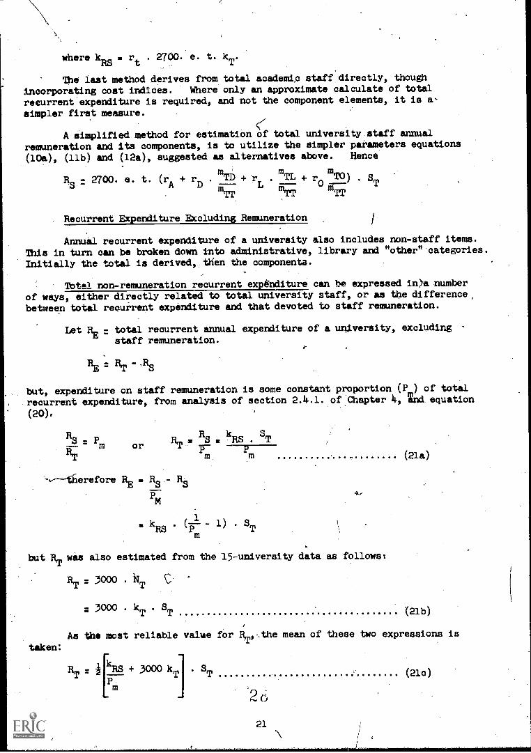
The last method derives from total academic staff directly, though

incorporating coat indices. Where only an approximate calculate of totalrecurrent expenditure is required, and not the component elements, it is a

simpler first measure.

A simplified method for estimation of total university_ataff annualremuneration and its components, 13 to utilize the simpler parameters equations(10a), (11b) and (12a), suggested as alternatives above. Hence

Rs : 2700. e. t. (rA -4- rD . mT0 -4-"r rOmT0) s

L TTT TT TT

Recurrent Expenditure Excluding Remuneration

Annual recurrent expenditure of a university also includes non-staff items.This in turn can be broken down into administrative, library and "other" categories.

Initially the total is derived, then the components.

Total non-remuneration recurrent ex 6nditure can be expressed inje number

of ways, either directly related to total university staff, or as the difference,

between total recurrent expenditure and that devoted to staff remuneration.

Let RE = total recurrent annual expenditure of a university, excluding

staff remuneration.

RE HT S

but, expenditure on staff remuneration is some constant proportion (P ) of total

recurrent expenditure, from analysis of section 2.4.1. of Chapter 4, ind equation

(20).

RS = Pm

"T

R k Slin, a S PIS T

or'

-+---wherefore RE R - RS

PM

RS. 1) . 3T

but RT was also estimated from the 15-university data as follows:

BT = 3000 NT c,

3000 . kT . ST

(21a)

'(21b)

As the most reliable value for RT,.-the mean of these two expressions is

taken:

{

RT = i :1.2 + 3000 kT . ST

m

(21c)

However total non-remuneration recurrent expenditure can also be writtenfrom column 2 of table 39, Chapter 4, as

RE x0 . e . NT

.e.kST T (22a)

incorporating cost indices for comparative purposes,

or RE z nRT . NT

= nRT kT ST (22b)

Taking the mean of the parameters linking recurrent non-remunerationexpenditure per annum (RE) and total academic staff (ST).

Let RE z kE . ST

and kE is the mean:

kE 1/6 [kT (3000 + 2nRT) +

and kRs z rT

.2700. e. t. k

e. t. kRS

(2 - 1 )]p--

or kRs - _ 1350 e. t. (rT kT + r0 k0 + rA + rD kD + rLL

. k.)

(22c)

This total non-remuneration recurrent expenditure per annum is distributedbetween administrative library, and "other" functions as follows:

LetRv-=total university annual recurrent expenditure excluding remunerationdevoted to administration £.s.e. (per annum).

REL =total university annual recurrent expenditure excluding remunerationdevoted to library £.s.e. (per annum).

RE = total university annual recurrent expenditure excluding remunerationdevoted to all other facilities £.s.e. (per annum).

Adminisration: RE'D = POD RE

= POD . kE .

Library: REh = POh RE

POh kE

REO = POO . REAll "other"

k .

00 E

ST

ST

ST

(23)

(24)

(25

222

where REDREL RED = RE

i.e. POD

+ POL

+ P00

1.

The distribution of recurrent expenditure (excludingthese items, in the 15-university survey, is set out in col'

remuneration) betweenumns 3-5 of table 15.

Total annual university recurrent expenditure is theand non-remuneration components.

ET . Rs + RE

sum of the remuneration

(26)

Note: In all cases above simplified values, based on those of (10a), (11b) and

(12a), consistently applied throughout the parameter calculations; canreplice the non-simplified values used above. In the following sections,

only non-simplified values are used. This involves substituting the

simplified forms for kD, kT'

etc., as appropriate.

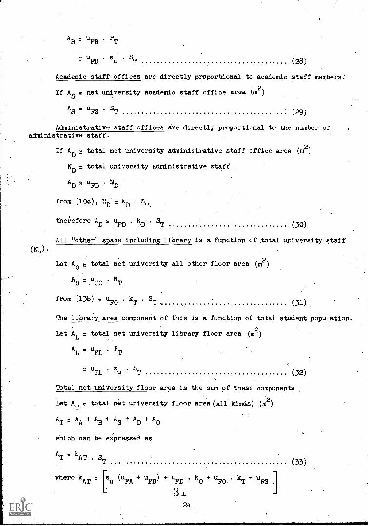
3.3. Net University Floor Area

The following two sections develop a methodology for calculating university

space requirements. In this section, university net building area is built upfrom the requireMents for separate categories of space, defined by their function.Hence the areas necessary for teaching rooms, laboratories, academic and \

administrative staff offices, library and "other" activities are'defined indepen

dently. The sum of these, net university building floor area, is then immediately

calculable. The relevant data analysis from the 15-university survey is found insection 2.3.2. of Chapter 14, with summary table 38.

Tb avoid excessive repetition, only non-simplified values are given in the

area sections following. However it is possible to substitute the simpler ratios

indicated above at the relevant points.

Teaching rooms'requirements are directly proportional to total student

population.

If. AA - total net university teaching rooms

PT = total university student populhtion

ST = total university academic staff.

then AA ureA . PT

but P s . S-T u T

where su

is the overall student /staff ratio.

then AA = upA su .

Laboratory areas

If AB

- total net university laboratory area (m )

LI

23

(27)

PT

uFB . su . ST(28)

Academic staff offices are directly proportional to academic staff members

If As = net university academic staff office area

A - u . SFS

ST

(m2)

(29)

Administrative staff offices are directly proportional to the number ofadministrative staff.

If AD

- total net university administrative staff office area

total university administrative staff.ND _

AD = uFD ND

from (10c), ND kD ST.

therefore A - u k . SD D T

(m2)

(30)

All "other" space including library is a function of total university staff

Let A0 = total net university all other floor area (m2)

AD r. uFO . NT

from (13b) = uF0 kT

ST (31)

The library area component of this is a function of total student population.

LetA_=total net university library floor area (m2)

AL uFL . PT

uFL su ST (32)

Total net university floor area is the sum of these components

Let AT = total net university floor area (all kinds) (m2)

AT AA + AB + AS + AD + AO

which can be expressed as

ATk

T AT . ST

wherekAT (uFA uFB ) uFD k0 UFO . kT + u

324

(33)

using equations (27) to (32).

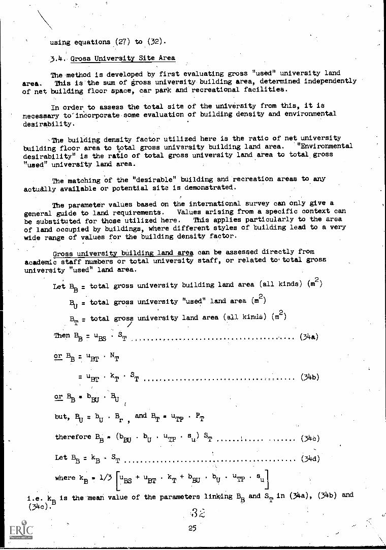
3.4. Gross University Site Area

The method is developed by first evaluating gross "used" university land

area. This is'the sum of grose university building area, determined independently

of net building floor space, car park and recreational facilities.

In order to assess the total site of the university fromthis, it is

necessary to'ineorporate some evaluation of building density and environmental

desirability.

The building density factor utilized here is the ratio of net university

building floor area to total gross university building land area. "Environmental

desirability" is the ratio of total gross university land area to total gross

"tame university land area.

The matching of the "desirable" building and recreation areas to.any

actually available or potential site is demonstrated.

The parameter values based on the international survey can only give a

general guide to land requirements. Values arising from a specific context can

be substituted for those utilized here. This applies particularly to the area

of land occupied by buildings, where different styles of building lead to a very

wide range of values for the building density factor.

Gross university building land area can be assessed directly from

academic staff numbers or total university staff, or related to,total gross

university "used" land area.

Let B8 r. total gross university building land area (all kinds) (m2

)

Bu s total gross university "used" land area (m2)

BT s total gross university land area (all kinds) (m2

)

Then B8 r. um . sm

or B8 = um . NT

= um . kT ST

(11: BB 4 bBUBU

but, Bu s bu . Br and BT a uTp . PT

therefore BB., (bEu . bu . uTp . su) ST(34c)

It BB s kB . ST (3d)

where kB a 1/3

[

uEs + uBT . kT + bEu . bu . uT, . su

.e.

kB is the mean value of the parameters linking BB and ST in (34a), (34b) and

(34c)B.

(34a)

(34b)

r:

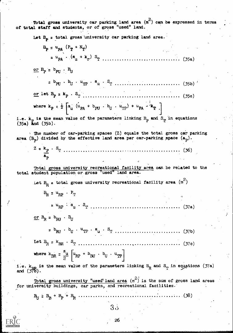
Tbtal gross university car parking land area (m2) can be expressed in terms

of total staff and students, or of gross "used" land.

Let Bp = total gross'university car parking land area.

Bp upA (PT + NT)

upA . (su + kr) ST (35a)

or Bp = bpu BU

= bPU bU P

su . ST(35b)

or let Bp = kp . ST.(35c)

where kp = [1.1 (upA + bpu . bu . uTp) + upA

i.e. k is the mean value of the parameters linking Bp and ST in equations

(35a) find (35b).

The number of car - parking spaces (Z) equals the total gross car parkingarea (Be) divided by the effective land area per car - parking space (ap).

Z - kP

. ST

Ap(36)

Tbtal gross university recreational facility area can be related to thetotal student population or gross "used" land area.

Let BR = total gross university recreational facility area

BR = uflp . PT

(m2)

= uflp su . ST

or BR = bflu .

BU

(37a)

b . bu . uTp . su

ST

.

RU (37b)

Let BR = km . STh

where k -su u + bflu . bu . uTpBR T RP

(37c)

i.e. k is the mean value of the parameters linking BA and ST in equations (37a)and (371) .

Tbtal gross university "used"land area2)

is the sum of gross land areasfor university. buildings, car parks, and recreational faCilities.

Bu B13 B1) BR

36

26

(38)

The total gross university land area oan be related to academic staff or to

gross "used" university land area (B6) ti

BT = .uTp su sT

A better value, based on a broad site-density factor is:

(39)

.7.. [1.1 ] . su

.. sT

N.]s TP 8

(39a)

where [1...11] = 55 for a high density situations = 2)0 for a low density situation

The alternative, incorporates a simple evaluation of "environmental

desirability".

Let BTD-

= - desirable "environmental limiting" value of BT, gross university land

area.

then BTD = 2.5 Et (40)

Building density ,criterion: building density can be considered separately

from the aggregated total site determinations. A building density factor is:

db = '1;P

BB(41)

which can be calculated directly froin equations (33) and (34c) for each university.

The total sample appears to fall into three separate density groupings sothat for an approximation it, can be deduced, that:.

-dB = 0.526 for a low average building density

1.664 for a meduim average building density

:2.749 for a high average building density

and these values can be used to indicate the order of building density for anycorresponding values of building floor area (AT) and land area (%).

4

Desirable recreational land area. As a "second order" factor inenvironmental desirability it would be advantageous to satisfy a recreationalland area criterion of the following order of magnitude (derived from column 4 of

table 37)

froth (37a), BR = uBp . su . ST

such that uRP

approaches 12,

or BAD = 12 . su . ST(4.2)

where BBD is the desirable environmental limiting value of recreation land

area,BR.

Practical Application

It is highly probable that calculated land values from the model will notsatisfy equation (33), or alternatively, that the land available is limited /anddoes not allow for total site to total "used" land area ratio of 2.5 (14.0).

In these cases, total site Bmro is fixed by circumstances external to the.

model. Given this total site, it Mpossible to proceed as follows:

Calculate the required net building floor space (Am) from equation (53).

Set an"envirdnmentally desirable" criterion for thetotal site relative tototal usable land. It is suggested here that this should be of the order of 2.5.(equation.(40)).

Calculate the total usable university land area (Bu) from equation (40).

Then:. BB = Bu - BR - Bp from (38). Gross university building area is hence

determined.

Calculate building density from equation (11.1) dB ATBB

Compare this value of dB to the set of values of building density - low,medium, and high - derived from the international averages, to indicate the orderof building density necessary for this site. If this is acceptable then the"environmental" equation (40) will be satisfied. If the density is unacceptablethen it will be necessary to modify the car parking area, Bo, and/or recreationarea Bo e.g. by the use of multi-storey car parks and high &ensity recreational

areas such aa "dry-play" surfaces.

As a "second order" environmental desirability it would also beadvantageous to satisfy the recreational land area criterion.

BAD 12. su . ST(42)

It is emphasized that the above method only gives an "order of magnitude"solution but it can be useful as an indication of desirable area distribution.

3.5. Total Capital Value and Annual Capital Expenditure

This is treated first as accumulated past capital expenditure, theexisting value of capital stock,'and second as a per annum expenditure in a growthsituation. The latter treatment includes an attempt to distinguish within annualcapital expenditure, that attributable to growth, and that which would be necessaryeven in a steady state - called the average annual basic or "true" capitalexpenditure.

Each of these types of capital expenditure are subdivided into building-andnon-building items. The growth situation presumes that the university institutionalready exists i.e. there is no analysis of expenditure requirement for a totallynew university.

Data analysis based on the international sample of 15-universities isdetailed in section 2.4.2. of Chapter 14., together with a more thorough appraisalof ."true"''or basic capital expenditure.

k )

Total Capital Value'

For all the followingit is assumed that student population, PT, is known.

Building

This entails assigning a monetary value to building requirements determined

in sections 3.3. and 3.4.,

From equation (33),-net university building floor area (AT) was related to

_total academic staff complement.

AT kAT ST

-AT T

where kAT

[su Ft uFA) uFD kA uF0 kT

uFS].

If k = constrUction2cost'per unit building net floor area (all kinds) in

£.s.e. per m ,

then the monetary value of the building capital (V is:

CB -k.k . SB AT T

All "Other" Capital Items

All other capital items are proportionately related to the capital value of./

(43)

buildings such that:

C0k . C

0 CO B

where C .. the value of all "other" capital items

6.= the ratio of the value of *11 "other" capital items to value of

buildings (C0)

5-

from (43), Co = kCO . k . kAT . ST(44)

Ibtal capital value of university is the sum of the capital values of

buildings and all other items.

C CB +T

-B

CO

= (1 +k ).k.k .SCO AT T (45)

where CT- the university total capital in £.s.e.

Annual Average Capital Expenditure

Within the total annual average capital expenditure, it is possible todistinguish between that associated with growth of the institutions, predominating

expenditure on building accommodation, other capital expenditure related to growth

and lastly a non-building "basic" capital expenditure which would be necessaryeven in a static situation. A method for the isolation, of these elements is

presented below. 3i)29

Building

It is assumed that there is an annual growth in student population of

APT = g, and that this value is known.PT

C - annual average total university growth capital expenditure onBg

building (£.s.e.)

CBg = g. k.

and from (33), g. k. kAT . ST

All Other Capital Expenditure

(1.6)

Using the growth,factor g it is possible to reduce capital costs other thanbuilding to a "basic" or "true" expenditure necessary in a steady state. This .

latter hypothesis is based on the assumption that the growth element in otherthan building capital can be removed by using a simple grOwth factor correctionas follows:

"Basic" average annual capital expenditure Cb = Co(1-g) (47),

where -Co - total average "other than building" annual capital expenditure.

If COg

. average annual total university capital expenditure, other thanbuilding, associated with growth.

then C =Og

g (48)

However basic annual average capital expenditure (unrelated to growth),Cb, is also related to academic staff numbers.

C - k . Sb D T

therefore COg

. ST

- g)

Total Annual Average Capital Expenditure

If CTg

= total annual average capital expenditure

then CTg

= CBg * COg

= g. k.k S+k. SAT 'TbT(1 g)

[

g. k. kAT + kb . ST

(1 - g)

(49)

(50)

4. Parameter Values deduced from the International Data

This section sets out the departmental and overall university constants,provided from the internatiOnal15-university sample and 80-university survey.Hence it provides two possible sets of values of the constants in'the simpleoverall model, which can be utilized to determine various resource requirements.The 'two sets of valuesareot directly comparable as the larger number ofobeervations in the 80university survey enabled a classification into 5 geographicalregions, contrasted to the 3 of the sample. However in many specific instances,the alternative values display a good degree of similarity.

The analysed results of the two surveys are presented separately. Tables 1,2 and 3 refer to the sample of 15, whilst tables 4, 5, and 6 refer to the full

80-university survey. Tables 1 and 4 detail the departmental constants whichcould be utilized for the evaluation of section 2 of this chapter. The methods

by which the raw data was analysed to arrive at these values is developed inChapter-41jections 2.1.2, and 2.1.3. Tables 2 and 5 detail the overalluniversity model primary constants, which can be used for the determination ofthe relationships of aection 3. Tables 4 and 6,provide the "secondary" constantsfrom which the former primary constants were derived. They hstve been incorpora-

ted at the appropriate points within section 3 of the model.

It is emphasized that these two sets of internationally derived data provideonly two possible sets of constants with which to evaluate the model. Alternative

sets, based on specific Local or national conditions, could equally as well beapplied.

Chapter 4, particularly section 2, provide more detailed analysis andinterpretation of the survey data, relevant to the overall simple model.

Section 5 of this chapter, utilizes the values of constants provided intables 1-3 (the 15-university sample results) to provide an example application

of the methodology.

3a

31

Table 1. --Values of Departmental Parameters - 15-University Sample

Vastron

.-..

Geog.

Group

Region

A

Acad/

1:tali.

(DA/DT

B

Teach

IAIIC:ci

Staff

(TT/

A)

C

lst/Tbtal

Teach Hrs.

'TT) *

D

Stud/

Acad

Staff

(FT/

A)

E

lst/Tbtal

Students

U/FT)

F

Recurrent

G

lbt. St.

H

Acad. Remun.

i.)t. Staff

°'1,,/ ,DT)

"Acad. Staff

(vA/D, A)

ilee:=.

( yk/v

.T)

1UK (3)

.521

9.34

.609

7.83

.811

3314

'.808

2819

Pure

NA (2)

.771

8.30

.635

4.75

,.549

3573

.831

3504

Sc.

EuR(8)

.529

8.10

.661

11.92

.843

2051

.801

2214

Av

.607

8.58

.635

8.17

.734

2979

.813

2846

2uK (o)

-

Archi-

NA (1)

.791

0.53

.393

.6.36

.424

3687

.818

3277

tect.

EUR(2)

.802

12.20

1.000

7q7

1.000

2604

.821

2358

Av

.797

6.37

.697

,6.87

.712

3146

.820

2818

3.

UK (2)

.519

11.34

.619

10.69

.829

2484

.811

2904

Tech.

NA ()

.549

1.97,

.295

7.48

.419

2790

.909

2960

EuR(3)

.579

12.70

.889

10.55

.984

2831

.709

2500

Av

.549

8.67

.601

9.57

.744

2702

.810

2788

4UK (1,)

.500

4.13

.611

3.66

.734

2487

.778

.2868

Med.Sc

NA (1)

.780

0.63

.700

13.47

.942

3732

.850

:,

3781

EuR(5)

:589

1.96

.376

15.74

.208

1898

.824

1963

Av

.620

2.24

.562

10.96

.628

2706

.817

2871

5ux (o)

-_.

-

Agric.

NA (1)

.625

0.57

.319

11.37

.721

30406

.932

3726

EuR(o)

--

.

Av

.625

0.57

.319

.11.37

.721

3006

.932

3726

4

Table 1 (Continued).

lassi-

ication

Geog

Group

AB

CD

EF _

GH

6UK (2)

.833

11.00

.916

10.00

.938

2371

.958

2563

Hum.

NA (3)

.837

10.08

.724

10.71

.354

3397

.912

3433

EUR 6

.784

.67

.682

11.0

.582

2186

.879

2429

Av

4.817

10.25

.774

10.60

.625

2651

.916

2808

--

Fine

NA (2)

.609

18.65

.828

5.64

.742

\ 2740

.855

3583

Arts

EUR(1)

.718

6.98

.696

15.21

.739

2551

.874

2607

Av

.664

12.82

.762

10.43

.741

2646

.865

2595

8UK (2)

'.696

11.19

0.000

5.81

.000

3.643

2500

Educ.

NA (2)

.780

20.31

0.425

23.26

.736

515

.83o

3026

(3)

.738

8.24

.617

12.38

.643

2180

.827

1956

Av

.738

13.25

.347

13.82

.46o

'2913

.767

2494

9UK (o)

-

NA (1)

.512

6.36

1.000

18.59

1.000

3326

.944

4545

EUR(6)

.739

11.88

.516

20.93

.667

2633

.895

2771

Av

.626

9.12

.758

19.76

.834

2980

.920

3658

10

UK (3)

.740

10.49

.737

9.12

.723

2595

.881

2725

soo.

NA (3)

.804

9.06

.610

,11.95

.754

3824

.829

2890

sc.

EuR(8)

.72o

7.11

.659

16.90

.784

- 2747

.780

2458

Av

.755

8.89

.669

12.66

'.754

3055

.830

2691

eVERALL

UK

.634

9.58

.582

.673

2716

.813

2730

7.8

AV

NA

.706

8.75

.593

11.59

.664

3359

.873

3473

EUR

.689

8.76

.677

13.57

.717

2409

.823

2362

ggregated Av.

.676

9.03

.617

11.00

.685

2828

.836

2855

The figures in brackets by UK, NA, etc. is

the sample number of classifications available.

Table 2.

Overall University (PriMy Constants) - 15-University Sample

Equation

No.

PriMary

Constant

10c

lle

12e

13b

15

16

17 19

19 22e

23

24

25

28

kD

kL

k0

kT RD

RL

kR0

1

W2

kE

POD

POL

P00

uFB FB

FB

Region

U.K.

N.A.

(30.579

o.o68to.007o.e

1.028-6.0035.%

2.675+0.-005.%

813 e.t.

(92+9.5.ede.t.

(991-3.4.eu)e.t.

(1896+6.1.eu)e.t.

[(1824-3.4.su)e.t.]

1.607-0.0035.su

(2528+3.3.su) +

(919+1.2.su) e.t.

1.670

0.060+0.0095.su

1.275-0.0047.0u

4.005+0.0047.su

5322 e.t.

(140+22.4.su)e.t.

(37001-9.2.su)e.t.

(9162+13.2.su)e.t.

[(9022-9.2.su)e.t.]

2.945-0.0047.su

(3548+4.2.5u) +

(1865+2.3.su) e.t.

0.057

0.1112

0.080

0.063

0.863

0.795

EUR.

AVERAGE

0.284

0.058+0.0033.su

0.550-0.0016.su

1.894+0.0016.su

375 e.t.

(81+4.6.su)e.t.

(923-1.8.su)e.t.

(1379+2.8.su)e.t.

[(1298-1.8.su)e.t.]

0.834 -0.0016.su

(1605+1.4.su) +

(5(38+0.5.su) e.t.

0.105

0.036

0.859

5_For a reasonable balance of disciplines

3 For an.arts/humanities bias

7 For a science/technology bias

0.493

0.055+0.0044.su

0.628-0.0022.eu

2.176+0.0022.su

826 e.t.

(84+6.8.su)e.t.

(1037-2.4.su)e.t.

(1947+4.4.su)e.t.

[(1863-2.4.su)e.t.

1.121-0.0022.su

(1917+1.9.su) +

(71.01+411-8rIps

) e.t,

-.1---

u

0.115

Table 2 Continued .

Equation

No.

Primary

Constant

Region

U.K.

N. A .

AVERAGE

27 29

30

31 32

33

31.1

35c

36

37c

39 39a

39a

44

49

uFA

FS

uFD

uF0

uFL

kAT

kB*

kP*

aP

k*

BR

1.4

18.4

16.7

31.9

-1.5

115.0+(uFBI-1.51).s

396 + 0.25.su

8.80 + 3.30.su

12

25.4

.su

256

2.0

18.1

1.0.1

43.1

1.7

209.5+(uF8 ±2.20).s

121 + 0.07.su

36.93

+9.26.su

15

19.8

.su

4196

2.9

22.1

34.6

49.7

0.8

124.0+(up:Bt2.89).su

157 + 0.07.su

5.21 + 2.75.su

12

3.3 .

s

80

2.3

20.2

26.6

-43.o

126.7+(uFB1-2.39).s

195 + o.09.su

9.51 + 4.38.su

13

13.2

.su

876

[ITP]s

1.11TP]s

dBdB

dB

55 Fbr a high density site situation

250 Fbr a low density site situation

0.526 signifies low building density

1.664 signifies medium building density

2.749 signifies high'building density

kC0

kb

0.471

836

0.266.

34o-

0.612

0.471

630

634

A value of kb

an

=is

approximate alternative overall value

*These constants have been modified from the original equations byignoring an excessively high parameter value

from one university (in a very small.sample) which was biassingthe numerical values.

Table 3. Overall University "Secondary" Constants - 15-University Sample.

(Used for evaluating primary constants)

Equat.No.

Sewn- Region

dart'

Constant .

U.K. N.A. EUR. AVERAGE-

mTA

0.21 0.40 0.15 0.20

10c [ mTT

0.37 0.25 0.52 0.46

mD

0.59 1.74 0.28 0.55 ,

11c mTL

0.05 0.03 0.06 0.05

11c mP

71.3 52.8 151.0 115.4

12c mTO

0.37 0.32 0.27 0.29

15 rD

0.52 1.18 0.49 0.62

16 rL

0.50 0.87 0.52 0.57

rT

0.65 1.21 0.84 0.87

17 [ r0 0.37 0_90 0.53 0.56

rA

1.050 1.230 1.030 1.140

rrrI

1335 1158 1042 1143

22c [ xo

1325 1960 1359 1457

pm 0.60 0.61 0.65 0.63

34d

uBS

uBT

420

139

121

- 30

159

82

208

83[

bBU

0.49 0.39 0.67 0.56

bu

0.251 0.437 0.394 0.369

35c uPA

3.29 9.22 2.75 4.37

37c uRP

25.4 19.8 3.3 13.2

44 eo

0.32 0.21 0.38 0.32

44 cB

0.68 0.79 0.62 0.68

36

Table 4. Departmental Conetantsl Classified by Region and Subject Area

80-University Survey

aubjeotClassifi-cation ,

Region

A

Aoademic/Total Staff(DA/

DT)

BTeaching Hrs4AbademicStaff(T.,,,

'IDA)

C

let Degree/Mortal Teaching

Hour*(Ty :

TT)

DStudent/Acad. Staff(FT

/D A)

E /let Degree//'Total Students(1?u/ /

FTy

///

.4F'

RecurrentExpenditure/Total Staff

(VT

D T)

0Total StaffRolm./Recurr.Expend.(V

NivT)

HAcad. Remuner./Acad. Staff

(V A/

nA),

N.A. 1 0.700 8.45 0.597 5.37 0.448 2750 4.00 2969

1. '

U.K. 2

acAAWANAviA 30.5500.527

9.985.23

0.7090.598

7.8758

0.8910.674

23732200

2.033.10

2802686

Pure Science "EEC" 4 0.594 _ - - - 2185 2,38 2112

OMB ZUA. 54 0.760 7.71 / 0.916 10.99 0.967 1714 1.81 2014

AMA= 0.610 8.C8 t 0.684 7.14 0.783 2340 2.77 2667

1 0.713 8.56 /,/

0.935 7.84 0.580 - 2771 4.00 2695

2. 2 0.577 22.001 0.927 11.13 0.976 2617 .3 .3. 3130

3 0.655 9.09 , LOGO 2550 3.45 2256Architecture 4 0.826 12;84 - 4.86 . - 2297 2.73 2248

5 0.724 11.66 - 8.88 0,845 1896 1.50 1902

AVERAGE 0.694t.13.51

i0.931 8.52 0.830 . 2493 3.03 2371

1 0.640 / 16.22 0.682 8.16 1.013 2861 ,3.86 2802

2 0.542 , 6.98 0.830 9.70 0.877 2425 2.10 2887

3. 3 0.474 // - 0.093 6.41 0.848 1786. 3.22 2614

Technology 4 0.634 9.96 6.16 - 2301 ' 2.56 2443

0.538 11.78 0.968 10.87 0.941 1864 1.41 1609_5

AVERAGE 0.563 9.56 0.784 8.19 0.911' 2332 2.58 2591

1 0.678 4.29 1.000 10.10 0.981 . 2836 3.62 2791.

2 0.488 6.77 0.857 4.58 0.813 2431 1.95 29314.

3 0.540 19.00 5.82 0.578 2253 3.18 270

Medical 4 0.493 - 4.42 5.464 1141 . 2.61 2312

3cienoes 5 0.774 7.43 , 0.654 7.92 0.785 1621 1.54 2188

AIMMAGt 0.607 8.14 0.762 6.53 0.950 2187 2.89 2519

1 0.607 15.89 0.504 11.07 0.774 2629 4.29 3154

5. 2 - - - - - - -

3 0.382 - - 5.76 0.981 2369 2.72 3016

Agriculture 4 - -

5 0.519 9.44 0.834 14.05 0.935 180 1.48 1852

AVERAGE 0.521 11.59 0.587 11.60 0.847 2192 2.66 2477

1 0.815 11.19 0.604 2.49 0.759 2454 4.40 300;

6.2

30.7400.802

10.006.04

0.8380.716

9.269.50

0.8860.685

21513061

2.333.27

.2531

3028

NUmanities 4 0.824 - - .20.26 0.878 2236 2.76 2273

5 0.806 6.78 0.961 12.67 0.978 2192 1.64 2057

AVERAGE 0.798 8.53 .0.762 11.35 0.807 2597 3.11 -,269)

1 0.795 18.71 0.824 8.16 0.835 2141 4.32 3232

7. '2 0.867 - - 6.31 0.878 2407 2.29 2546

Fine Arta3 - - - - 0.739 -

5 1.000 9.50 1.000 14.50 1.000 - - 2108

AVERAGE 0.829 17.40 0.849 9.66 0.863 2208 3.81 3006.

1 0.716 11.50 0.667 20.49 0.853 2870 4.02 2785

8. 2 0.650 9.75 0.846 10.64 0.098 2236. 2.30 2700

Education3 0.728 - 0.500 15.85 0.882 3139 3.23 3476

0.800 6.25 0.400 7.08 - - 26u

AVERAGE 0.710 10.10 0.624 15.75 0.782 2770 333 2917'

1 0.420 5.88 1.000 15.77 0.679 3284 3.6o 3981

9. 2 - - - - - - -

Law34

0.7990.755

9.79-

0.766-

17.7238.54

0.657- ,

26662479

3.422.90

29682514

5 0.756 6.23 1.000 82.09 1.000 1851 1.55 1886

AVERAGE 0.720 7.48 0.867 31.29 0.684 2669 3.11

1 0.70e 10.73 0.625 17.65 0.743 2870 4.11 3177

2 0.796 9.40 0..860 9.12 0.813 2427 2.28 263310.

3 0.776 5.80 0.519 17.68 0.812 2562 3.24 2675

Social 4 0.904 - - 17.18 0.668' 2571 . 2.89 2640

'Sciences 5 0.816 7.70 0.882 14.53 1.04 1855 1.25 1985

AVERAGE 0.769 8.93 0.695 15.23 0.840 2593.. 3.16 2722

emu' 0.674 9.16 0.728 11.41 0.828 2438 2.91 2669AM OS

L

37

.Table 5.

Overall University - Primary Constants

84-University Survey

Primary

Constant

Region

1. North America

2. United Kingdom

3. Scandinavia

4. Predominantly EEC

5. "Other" European

AVERAGE

10c

110

.2c

13b

15

16

17

19

19 2 50

70

kR

kRD

kRL

kR0

1 2

P OD

POL

P00

uFB

uFA

UF$

uFD

UFO FL

k AT

kB

k *

kBR

TP

[IITP]s

dB

IkCO

kB

1.001

0.138 + 0.006.su

0.821 - 0.003.su

2.960 + 0.003.su

1195 e.t.

(168 + 7.0.su)e.t.

(1168 - 2.6au)et

(2531 + 4.4.s )e.t.

(2363 - 2.6.8u)a.t.

1.822 - 0.0029.mu

(9184 + 9.0.su) +

(6213 + 6.1.su)e.t.

0,215

0.072

0.816

4.06

1.51

13.93

12.63

41.76

2.20

150.2+(upB+1.63).au

310 + 85.378u

13.09 + 78.98.8

159.8.su

1852

1.17

8

0.518

0.459

0.051 + 0.005.mw

0.47 + 0.003au

1.054 - 0.003au

0.649 - 0.002su

2.622 + 0.003su

2.154 + 0.002.au

641 e.t.

513 e.t.

(62 + 6.4.au)e.t.

(52 + 3.6.au)e.t.

(1033 - 2.3.au)e.t.-(850--

(1736 + 4.2.au)e.t.

(14-1.4 + 2.4.su)e.t.

(1674 - 2.3.8u)e;

(1362 - 1.2.su)e.t.

3.571 - 0.0026f,au

(3737 + 3.7su) +

(765 + 0.8.su)e.t.

0.062

0.058

0.881

5.77

1.79

14.46,

15.50

25.15

1.74

88.4+(uFB+1.85).su

262 + 15.36.au

10.26 + 8.32.su

44.1.8

192

0.90

8

3.108 - 0.0016.a

(3139 + 2.4.au) +

0.7.su)e.t.

0.108

0.077

0.849

5.85

3.37

17.29

25.90

26.61

12.85

8674.(uFB+3'41)*%

165 + 48.65.su

2.89 + 16.44.su

78.0.su

485

(934

- +

1.05

7

0.278

0.053 + 0.004au

0.450 - 0.002.au

1.782 + 0.002.au

328 e.t.

(72 + 5.1.au)e.t.

(652 - 1.9.cde.t.

(1051 + 3.3.au)e.t.

(979 -

0.729 - 0.0019.3u

(2861 + 3.0.su) +

(792 + 0.9.su)e.t.

0.075

0.078

0.872

8.56

2.70

20.38

15.21

40.46

1.17

96'7+(uFB-1-2.78)su

72 + 11.64au

0.28 + 6.39.su

19.0.au

118

1.90

5

0.213

0.023 + 0.001su

0.390 - 0.0004.8

1.626 + 0.0004.15u

232 e.t.

(20 + 0.7.su)e.t.

(381

0.3.su)e.t.

(632 + 0.5.su)e.t.

(613 - 0.3.su)e.t.

0.603 - 0.0004.au

(2332 + 0.6.su) +

(478 + 0.1.su)e.t.

0.107

0.076

0.865

8.83

3.65

14.32

55.28

193.51

0.54

340.8+(uFB+3.73).8

946 + 20.62.su

8.99 + 9.68.su

48.9.su

197

1.32

3

0:477

0.056 + 0.004.8 u

0.659 - 0.002.su

2.192 + 0.002.a u

552 e.t.

(66 + 4.2.8u)e.t.

(820 - I.5.su)s.t.

(1437 ± 2.7.su)s.t.

(1372 - 1.5.su)e.t.

1.136 - 0.0018.su

+ 3.2.su) +

(1500 + 1.4.su)s.t.

0.109

0.073

0.852

6.34

2.73

16.15

26.59

67.80

5.91

13311+(uFB+2.95).su

298 + 40.30.su

5.68 + 21.10.su

(383

2 72.4.su

572

1.19

8

Table 6.

Overall University Secondary Constants - 80- University Survey

(Used to evaluate primary constants).

Squat.

No.

-..

Region

Secondary

Constant

1. North

America

2". United

Kingdom

.

3. Scandinavia

4. Predominantly

EEC

'

5. "Others ".

European

AVERAGE --,

10c

11c

lic

12c

15 16

17

22c

34d

35c

37c

44

44

mTD

m

[

TT

mu

MTL

mP.

mT0

rD

rL

rT

r0

[rA

11RT

L

xo

Pm BS

I

u

BT

bEu

bU

uPA'

uRP

CO

CB

0.31

0.33

1.06

0.09

86.60

0.26

0.43

0.44

0.64

0.41

.0.91

7808

6409

0.54

411

176

0.41

0.34

8.85

64.1

0.19

0.38

0.53

0.04

95.39

0.39

0.45

0.44

0.62

0.36

1.00

2776

1157

o.6o

415

141

0.40

c.6o

7-83

42.5

0.19

0.46

0.50

0.04

154.67

0.30

0.40

0.40

0.65

0.39

0.83

2871

1795

0,70

267

105

0.65

0.47

2.68

10.3

0.15

0.55

0.28

0.06

132.27

0.24

0.42

0.49

0.72

0.45

o.86

3318

1756

0.64

114 58

0.29

1.00

0.31

3.2

.0.13

0.61

0.22

0.03

-

591.89

0.23

0.39

0.31

0.50

0.34

0.58

2802

969

0.53

1612

753

,

0.73

0.43

11.05

36.3

0.19

0.47

-0.51

0.05

194.61

0.29

0.41

0.41

0.63

0.39

0.84

3594

2248

0.63

578

253

0.56

0.48

6.41

32.3

5. Example Application of the Methodology

In this section an exaMple application of the methodology is presented,based on parameter value* obtained in the 15-university sample, and set out intables 1, 2 and 3 of section 4 above. This university is compared with the"overall average" university. Alternative parameter values, for example for the80-university survey, ooul&be substituted at the relevant points in the methodo-logy to.obtain an alternative set of approximations.

University X - Input Data.

Table. 7. Departmental Student Data - Example

Classifi-cation No.

Subject Area

StudentslstDegreeFUi

StudentsHigherDegreeFGi.

Tbtal (F x

Ti)

. (FUi

+ FGi)

1 Pure Sciences 1311 850 2161

4 Medical Sciences 113 77 190

6 Humanities 1647 893 2540

8 Education 206 43 219

9 Law 1274 959 2233

10 Social Sciences 510 177 687

TOTALS 1 5061 2999 8060

Origin of X: It is aasumed that University X is from Holland in the Europeangrouping. Hence.:

e a 8.69 t =.0.0967 k = 57.6. ZOISIDee

Growth: Assumed to be at the rate of g 15% per annum

Data at subject level

Using Table 7 and the oonstants from section 4, table 1, the followingbasic calculations can be made:

40

Table 8.

Departmental Calculations - "UniversityX" "Average University"

Equation

v

la

lb

ic

35

67

C.

lassif

po. (1)

Univ

Staff Teaching

ours - 1st

.egree

Till

Staff Teaching

hours - all

higher degrees

T Gi

Total Staff

weekly

teaching

hours

TTi

Departmental

Academic

Staff

D Ai

Departmental

Total Staff

DTi

Recurrent

Expenditure

per annum

VTi

Recurrent

Staff

Remun.

per annum

VNi

Recurrent

Academic

Staff

Remun.

per annum

V 'Ai

£.s.e. x 10-

1X Av.

697

1192

1247

1225

1944

2417

240.0

281.7

453.7

464.1

931

1383

746

1124

538

802

14

X Av.

25

23

8

19

33 42

19.o

18.8

32.3

30.3

61 82

5o

67

37

54

6x Av.

1683

1973

592

751.

2275

2724

235.3

265.8

a..

300.1

325.3

656

862

577

790

572

746

8x Av.

132

149

31 50

163

199

19.8

15.0

26.8

20.3

'

58

59

48

45

39

37

9x Av.

559

534

791

666 .

1350

1200

113.6

131.5

153.7

210.1

405

626

362

576

315

481

10

X Av.

181

318

118

167

299

485

42.1

54.6

58.5

72.3

161

221

126

143

10

147

x Av.

3277

'

4189

,2787

2878

,

6064

7067

669.8

767.4

1025.1

1122.4

2272

-

3233

1909

2785

1604

2267

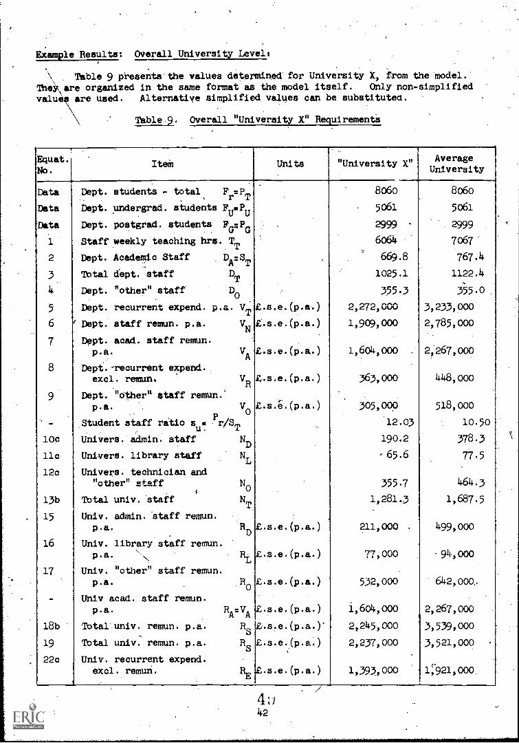
Example Results: Overall University Level:

Table 9 presents the values determined' for University X, from the model.The'SX,are organized in the same format as the model itself. Only non-simplified

value are used. Alternative simplified values can be substitutech

Table 9. Overall "University X" Requirements

IteMNo.

Units "University X"AverageUniversity

Data Dept. students - total Fr P. T

8060 8060

Data Dept. undergrad. students Feu - 5061 5061

Data Dept. postgrad. students FG:PG 2999 2999

1 Staff weekly teaching hrs.TT 6064 7o67

2 Dept. Academic Staff D -A-

ST

669.8 767.4

3 Total dept. staff D T 1025.1 1122.4

4 Dept. "other" staff0 355.3 355.0

5 Dept. recurrent expend. p.a. VT £.s.e.(p.a.) 2,272,000 3, 233,000

6 Dept. staff remun. p.a. VN

1,909,000 2,785,000

7 Dept. acad. staff remun.p.a. VA Z.s.e.(p.a.) 1,604,000 2 267,000

8 Dept.-recurrent expend.excl. remun. VR fos.e.(p.a.) 363,000 448,000

9 Dept. "other" staff remun.'p.a. V

0305,000 518,000

Student staff ratio s Pr /STu. T

12.03 10.50

10c Univers. admin. staff ND

190.2 378.3

11c Univers. library staffL

- 65.6 77.5

12c Univers. technician and"other" staff NO 355.7 464.3

13b Total univ, staff NT

1,281.3 1,687.5

15 Univ. admin. Staff remun.p.a. R

D£.s.e.(p.a.) 211,000 499,000

16 Univ. library staff remun.p.a. RL £.s.e.(p.a.) 77,000 -94,000

17 Univ. "other" staff remun.p.a.

0

Univ acad. staff remun.

Z.s.e.(p.a.) 532,000 642,000,

p.a. RA=VA

£.s.e.(p.a.) 1,6o4,000 2,267 000

18b TOtal'univ. remun. p.a. RS 2, 245,000 3,539,000

19 Total univ. remun. p.a. RS 2,237,000- 3,521,000

22c Univ. recurrent expend.excl. remun.

RE£. s.e.(p.a.) 1,393,000 1;921,000

41)42

Tale Continued

E4uat.No.

Item\

Units "UniversityUniversityAverage

University

23 Univ. recurrent expend.excl. remun. (admin.) RED

s.e.(p.a.) 146,0oo 221,000

24 Univ. recurrent expend.excl. remun.-library REt . ..:(p.a.) 50,000 94,000

25 Univ. recurrent expend.excl. remun.-"other"

,

REO£.s.e.

6. .)1,197,000 1,606,000

26 Univ. total recurrentexpend. p.a. RT E.s.e.(p. ) 3,,638,000 5, 460,000

27 Net univ. floor area -teaching AA m

223,400 18,500

28 Net univ.,floor area - 2labs. AB m 32,200 32,200

29 Net univ. floor area - 2 (*)

acad. offices As m 13,400 15,400

30 Net univ. floor area -admin offices AD m

2 6,600 10,100

31 Net univ. floor area -"other" A0m2

63,700 72,500

32 Net univ. floor area -library AL m

26,500 9,700

33 Net univ. floor area Ar m2

139,300 148,700

34d Gross univ. building area BB m2

105,700 105,300

35c Gross univ. car park area m2

25,600(d) 42,600(d)

36 Approx.Iro. of car spaces Z spaces 2,137 4,259

37 Gross univ. recreation area Bili mP 26,600 106,400

40 "Desirable" value of BR %111 m2 96,700(c) 89,300(c)

38 Grosuniv. "used" land2

area BU m 157,900 299,300,

39 Gross univ. land area BT

m2 644,6o0 7,058,500

39a [BT]s highm2 443,200(a) 443,200(a)

39a- [Bo low2m 2,014,400 2,014,400

41 Building density factord

AT/BB1.318 0.989

(meduim (meduim/low

2density) density)

38 Gross univ. land area BU m 228,000 282,000(using 40 in-stead of 37cin 38)

40 'besirable" value of BT

BTD

394,800 748,300

(*) An interpolated value u-i

4-0 ir; use1 here.rA

t) t1

43

Table 9 (Continued).

uat.

.

Item UnitsUnits "University X"Average

University

or 570,000(b) or 705,000(b)Note that (a) does not satisfy

40 Gross univ. land area(b)

177,200 I 177,200(Using values (a))

38 Gross univ. building area BB a2

, 54,900 1 45,300(Using values (c) and (d))

41 Building density factor dB 2.5371 3.28(High building density. In-vestigate alternative parkingand/or recreation areas).

43 Capital value of total univ.building C

B£. s.e.(total) 7,984,000 9,191,000

44 Capital value of total univ.other than building C

o£.s.e.(total) 4,886,000 4329,000

45 Tbtal'univ. capital CTZ.s.e.(total) 12,870,000 13,520,060

46 Univ. growth capital onbuilding C

Bg£.s.e.(p.a.) 1,204,000 1,378,000

49 Univ. growth capital onother than building C

OgZ.a.e.(p.a.) 378,000 433,000

50 Av. univ. growth capital-total CTg E.s.e.(p.a.) 1,582,000' 1,811,0p014.9Av. "basic" capital expend. Cb £.s.e.(p.a.) 322,000 368,000

14.14.

Table 10. A Selected Summary of Results (Costs in Currency of "University X")

University "X" and Average University

Item Units "University X"AverageUniversity

Pure Science Subject Area

Tbtal students 2161 2161

Total academic staff 240.0 281.7

Total staff 453.7 464.1

Total annual staff remuneration Guild.p.a. 7869000 12364000

Total annual recurrentexpenditure Guild.p.a. 9589000 15213000

Humanities Subject Area

Total students 2540 2540

Total academic staff 235.3 265.8

Total staff 300.1, 325.3

Total annual staff remuneration Guild.p.a. 5943000 8690000

Total annual recurrentexpenditure Guild.p.a. 6757000 948200o

Total University

Tbtal students 8060 8060

Total academic staff 669.8 767.4

Total staff,(all kinds) 1281.3 1687.5

Total admin. staff annualremuneration Guild.p.a. 2173000 5489000

Library recurrent lessremuneration expenditure Guild.p.a. 515000 1034000

Tbtal staff annual remuneration Guild.p.a. 23124000 38929000

Total recurrent annualexpenditure Guild.p.a. 37471000 60060000

Total laboratory net floor area m2 32200 32200

Total building net floor area m2

139300 148700

University members per car park

space 4.37 2.29

Total used land area m2

157900 299300

Total site land area m2

443200 443200

Desirable site land aream2

570000 705000

Average annual growth buildings

capital Guild.p.a. 12401000 15158000

Tbtal average annual capital Guild,p.a. 16295000 19921000

45OA,

CHAPTER 3. A CONCEPTUAL METHODOLOGY FOR THE DETERMINATION

DI DEPARTMENTAL REQUIREMENTS

1. Introduction

2. Academic Staff Estimation

2.1. Basic Methodology

2.1.1. The Generalized Programme of Study Concept

2.1.2. Academic Staff Contribution to Various Programmes

2.1.3. Incorporation of Service Teaching

Page No.

48

48

48

49

51

52

2.1.4. Tbtal Departmental Academic Staff Requirementand its Composition 56

2.2. Initial Simplification of the Equations

2.3. Application to a Typical U.K. University

59

63

3. Estimation of Departmental Technical Support Staff 70

3.1. Basic Methodology 71

3.2. Departmental Support Staff 73

3.3. Example Application to a Typical U.K. TechnologyDepartment' 74

4. Estimation of Departmental Administrative Staff 74

4.1. Basic Methodology a 74

4.2. Example Application to U.K. Universities 78

Appendices

Al: Weighting of Fundamental to Advanced Level Students

A2: Relationships between Departmental Academic Staff,Support Area and Support Staff

r-

47

79

8l

1. Introduction

The methodology developed here has as its goal the determination ofacademic, technical support and administrative staff at the departmental levelof university type institutions. The approach is a combined conceptual /dataanalysis one and would provide reliable intra-university data although it can beused in aggregated form for institutional r,equirements (see reference 5).

The method has been developed to be as flexible as possible so that itcan, be applied interAatiorially. Thus a basic concept of programmes of studyat defined levels of study has been introduded, from which springs specificequations for departmental academic staff for particular geographical regions.It fs thought that this basic concept is applicable to other foma of organizationthan the common faculty-department-arrangement. Such application is left tothe reader.

The basic. concepts for academic staff analysiaare described. Theseare then developed .for departments in general terms from which practicalevaluations are" acilitated using data based parameters which vary by subjectclassification and by geographical region. A comprehensive example is givento illustrate the application of the complete method.

. The determination of supporting staff (technicians, assistants, etc.),and administrative staff depends upon a reasonably accurate estimate of acadethicstaff distribution.' The former is also found to depend significantly oneffective "laboratory", area and hence an analysis of this is also developed interms of academic staff.

The whole approach is kept as,simple as possible as the objective is toprovide methodology and useful data to enable individual universities to developtheir own specific equations and methods. Decisions on method and data constraintsshould spring from bodies which include academic staff, students and administra-tors.. However it should be added that the appendices of this chapter, andChapter 4, contain a considerable quantity of general information, which can beof use in solving specific academic planning problems.

2. Academic Staff Estimation by Department

2.1. Basic Methodology

The functions of academic staff can be broadly described as follows:

(a) Teaching Function: First degree or diploma, higher degree ordiploma, short specialized 'programmes, research supervision andindustrial, visiting to students (where "sandwich" or co-operativeprogrammes are involved).

(b) Personal research and "consultancy function".

(c) Other Functions: 'Administx:ation, committees (university,professional and national), student counselling.

The assessment of academic staff requirements presented here takes intoaccount only the teaching function. It has been. reasonably well establishedwithin arl international framework that average staff/student contact teachingloads are of the order of 9-10 hours/Week (with a factor of about 2.5 forconversion to.stetual worked hours - allowing for preparation, marking, etc.)and that personal research and consultancy occupies 25-30% of a normal working

5,i48

week. This accounts for about 36 working hours per week with say, at least four

hours per week for the other functions. Thus on this basis it is assumed

justifiable to concentrate on the teaching function to define the staff requirement

for a university or department - the remaining time being available for research

and other,functions. This definition must, of course, be based on the average

staff member and does not imply that every staff member proportions his time in a

uniform way. Having established a staff requirement based on the overall teaching,

function commitments in a reasonably equitable ay it is a matter of detailed

management within the university and its o anizational structure to determine the

individual functions of its academic staff.

Thus the method oz staff estimation is based on the teaching function which

is, in any case, the basic "raison digtre" of a university.

2.1.1. The Generalized Programme of Study Concept

Departmental teaching responsibilities can be analysed via the utilization

of a generalized programme of study concept. A Oogramme of study is defined as

those requirements which must be satisfied for the satisfactory completion of the

student's period in the university. It frequently is terminated by the award of

a degreeor diploma. Thus the concept embraces all the teaching functions of

the department - undergraduate courses, student research work, short courses,

industrial training etc.

Each programme will generally include lecturing, seminar, and/or project/

thedis commitments. Each programme is further classified by the levels of study

incorporated. A study of various systems of university education across nations

suggests that academia work can be defined at three levels of study:

Level 1: Fundamental. Early first degree/diplOma study

Level 2: Advanced. Intermediate. between first degree/diploma andhigher degree/diploma study.

Level 3: Higher. Higher degree/diploma study.

Two particularly cliff-Inuit probleme regarding the choice of approach were

encountered. The first concerned the decision as to whether the basic approach

should derive fgpm subject elements or from complete programmes of study. The

second, connected, problem was that of making adequate allowance for service

teaching between departments. The generalized programme of Study was finally

selected as all students must eventually ,satisfy a particular programme to

qualify for a specific degree or diploma.

Departmental servicing 'contributions are incorporated through the use of

distribution factors which are developed in some detail (as it is often here in

practical application that the greatest emotion is generated inter-departmentally).

for the departmental teaching, function,fundamental, advanced, and higher. From

types of study programmes, e.g. shorttypes of study programmes are detailed

Hence a general equation is derivedin terms of different levels of study -this simplified expressions for particularcourses, are easily evolved. The various

individually.

At this stage it is not possible to simplify the equations further because

of differing programme structures and approaches at the international level. It

is, however, possible to provide considerable data reduced parametric information

r-

19

for specific geographical regions and subject classifications and these can beused in the generalized equations which can then be conditioned to the particular-university teaching function. In order to illustrate the WC application of themethOdo therefore, the equations are developed for typical university in theUnited Kingdom and worked examples are given for a typical technology department

. in which academic staff estimations are made for first and higher degree pro-grammes, (including a detailed estimate of servicing distribution factors), short'courses, research supervision and industrial visiting.

Principal Notation.

1 1' 12, 13 ,

sl, s2,

gl' g2, g3

P1' P2' P3

wl' w2, w3

Y1, Y2, Y3

k1, k2, k3

P PP

p33

b2' -3

h1

hs

w

S

SD

DA

Ss

SR

M11

- average student lecture hours/week at study levels 1, 2, 3.

- average student seminar hours/week at 'Study levels 1,.2, 3.Seminar hours are all hours spent in the classroom,excluding'lectures.

- average student seminar group sizttat study .levelealaaThis is the average size of all teaching groups, excludinglectures.

- total student numbers in a prograurne'at study levels 1,

7- total number of weeks tuition at study levels 1, 2, 3.

- number of years in a programme at ,study levels 1, 2, 3.

- weighting factor on staff loading relative to thefundamental level (1) at study levels 1, 2, 3.

- total student numbers on project/theses at study levels 2, 3.

- average weekly staff hours per student of projectsupervision at study levels 2, 3.

- average weekly staff hours per student of thesis supervision

average.leaturing staff hours /week at fundamental level ofstudy (1).

- average seminar staff hours /week at fundamental level ofstudy (1).

- number of weeks in university academic year

- academic staff requiremants for a generalized programmeof study.

- total departmental academic staff' contribution to aprogramme of study.

- total departmental academic staff requirement

- departmental academia staff requirement for short courses

- departmental academic staff requirement for researchstudent supervision

50

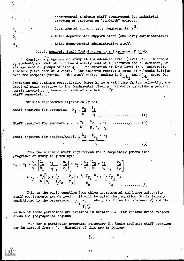
ST

DS

- departMental Academic staff requirement for industrialvisiting of students on "sandwich" courses.

- departmental support area requirements (m2

)

- total departmental support staff (excluding administrative)

- total departmental administrative staff.

2.1.2. Academic Staff Contribution to a Programme of Study

-Consider a progrnmme of study at the advanced level (level 2). It enrols

P2students, and each student has a weekly load of 1

2lectures and so seminars, in.

average seminar groups of size g2. The duration or this level is Y2 universityacademic years each of w weeks. The students receive a total of w

2weeks tuition

over the complete period. The staff weekly loading is hlyl, and hs hours forf-2

lecturing and seminars respectively, Where k2

is a weighting factor reflecting thelevel of study relative to the fundamental level p students undertake a projectthesis involving b

2hours per week of academic Pr

staff supervision.

This is represented algebraically as:

Staff required for lecturing = k2 . w2 . 12

w h1 (1)

Staff required for seminars = k2 . w2 82 . P2 (2)

w g2 .hs y2

Staff required for project/thesis = k2 Pp2 b2

h8 (3)

Thus the academic staff requirement for a completely generalizedprogramme of study is given byfN,

S = k . wl 11 + 81 . P1 + k . w2 12 + 8.2 . P2y 1 i;-- ---= 2

gn Y 452

77.hy2-;--

is 1 8

p+ k.,

p.

w3

13 +

s3 . 3 + k2 p2

b k p b2 + 3 p3 3

[' w hi. g3h y3 \

hs

hs (4)

This is the basic equation from which departmental and hence universitystaff requirements are derived. It Will be noted that equation (4) is largelyconditioned by the parameters 11/h

s1

etc., and b(As in reference 2) and the1g1hs

values of these parameters are examined in section 2.2. for various broad subjectareas and geographical regions.

Thus for a particular programme structure the basic academic staff equationcan be derived from (4). Examples of this are as follows:

51

let Degree in the U.K.

Normally this would,embrace 2 years at fundamental level and 1 year atadvanced (i.e. a total of 3 years).

Typical values would be:

w1 /w = 2 yl = 2 w2/w = 1 y21

(All third higher level would be zero).

Thus:

S = k + sy 1 1 1

h1

g1hs

. p1 + k 2[1, 2 + s2

h h1 -2 s

pr] + k2 pp b2

hs

Higher (masters) degree in the U.K. by course:

5 1: 52 y

3= 1 p = p

5(all others zero).

P3

Sy = 2

3k3 [ 3 + s3 . p3

,] + k_ p

P,. b3

h1

g3hs J

hs

1st Diploma in a European University

Normally this would embrace 3 years at fundamental level and 2 years atadvanced (i.e. a total of 5 years).

Typical valuep would be:

wi/w = 3 yl = 3 w2/w = 2y2 = 2 (see third level zero)

Sy

= k1 1

+ s1

k2

212+ s

2 k2 pi'. b2

hl glhs Pl] h1

g2hs

P2]2

hs

Other variations are apparent but the above examples serve to indicate theflexibility of the generalized programmP of study concept.

2.1.31 Incorporation of Inter-Departmental SerVice Teaching

In general any programme of Gtuc3y will be serviced by a number ofdepartments although it will almost certulnly be attached to a particulardepartment for organizational purposes and will be in the general subject area ofthat department.

Thus each department servicing a programme of study requires a proportionateallocation of staff. This is achieved here by developing departmental academicstaff,distribution factors for the generalized prOgramMe of study.'

52

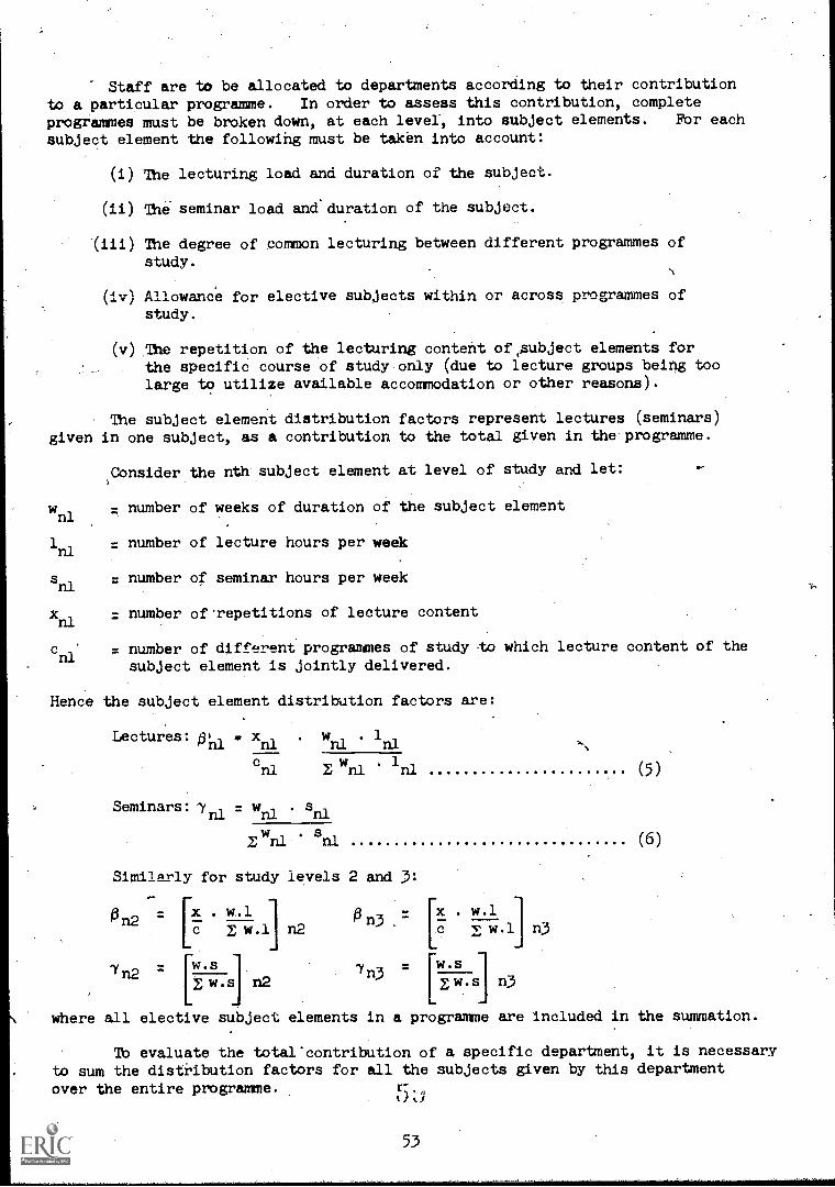
Staff are to be allocated to departments according to their contributionto a particular programme. In order to assess this contribution, completeprogrammes must be broken down, at each level, into subject elements. FOr each

subject element the following must be taken into account:

(i) The lecturing load and duration of the subject.

(ii) The seminar load and duration of the subject.

The degree of common lecturing between different programmes ofstudy.

ti

(iv) Allowance for elective subjects within or across programmes ofstudy.

(v) The repetition of the lecturing content ofisubject elements forthe specific course of study only (due to lecture groups being toolarge to utilize available accommodation or other reasons).

The subject element distribution factors represent lectures (seminars)given in one subject, as a contribution to the total given in the programme.

Consider the nth subject element at level of study and let:

wnl

= number of weeks of duration of the subject element

1nl

= number of lecture hours per week

= number of seminar hours per weeknl

nl= number of.repetitions of lecture content

nl m number of different programmes of study tto which lecture content of the

subject element is jointly delivered.

Hence the subject element distribution factors are:

Lectures: ona . xna . wna . 1n1

w . 1nl nl 1n1 (5)

Seminars: ^yra = wnlsnl

w snl n1

Similarly for study levels 2 and 3:

[On2 " x 14'1 0 n3 = lc /11--

c m w.1] n2 c v w.1 n3

'Yn2 = w.s'Y n3 w s

E w .s n2 z w . s n3

(6)

where all elective subject elements in a programme are included in the summation.

lb evaluate the total' contribution of a specific department, it is necessaryto sum the distribution factors for all the subjects given by this department

over the entire programme. r;.,

53

If j1

subject elements at level 1 in the programme of study are contributedby one department then the departmental distribution factor is:-

Lectures: 01 = z

Seminars:

(7)

1 = 1 nl (8)

Similarly for levels of-study 2 and 3:

132 = 2 °n2 °3 = / 3 In3

2 = z. j 2 7 n2J3

73 "

Then the total departmental academic staff contribution to a programmeof study is

SD k . wD 1 1

w

+ k3

. w3

1 + s1 1 1 1

h1

w2,/r212

w h1

. 1 + s_

3T3 PL._

+ k2pP2

. b2

h1

g3 s

y3 h

s

NOTE: p and p migiit need toP2 : P3

departments. In generalorganizing the particular

study:

. s2

g2 hs y2

k3 . b3

s ....... (9)

be modified is projects/theses are shared across

they will be supervised by the departmentprogramme of study.

It will be observed from (4) and (9) that for a complete programme of

rst = E 'Y2 _ E 'Y3 1

that is, in the Case of seminars, the sum of staff allocated in this mannerbetween contribUting departments, equals the total required for the programme.This is as logically expected.

However Z101, 10'2 and E.0 will only equal unity if there is no repetitionof lectures Within -a programme ( -"the influence of x) or no cOmmoh lecturingacross programmes (the influence of c). These latter will respectively increaseor decrease the value of E from unity if they occur.

These equations are perhaps mare easily understood by reference to thefollowing table 11 which illuetrates a method of-calculation of the distributionfactors for the fundamental level of a programme of study (tables 4 and 5 ofsection 2.3. also present a practical calculation with typical values).

The importance of allowing for servicing is demonstrated in section4.3. of Chapter 4 which indicates average inter-faculty servicing up to 30%and over 50% where faculties are largely professional (e.g. agriculture andforestry).

Table 11.

Programme of Study Distribution Factors

Level

Fundamental

Dept.

Subject

Element

n

Lecture

Repetition

x-

Common

Lectures

c

Duration

weeks

w

Lecture

hours/

week

1

Seminar

hours/

week

s

w.1

w.s

0

sel

1 2 n J...

...,

..

cn1

e

..

..

..

..

.,

..

..

.. [wA

nl

..

..

.

..

..

..

..

r.

xni

.wnl

.1nl

7n

:wnl

.snl

1 for Dept z.1

.1

7 lz.1

z w.1

z w.s

z.2

..

..

..

...

..

..

..

..

..

..

..

..

..

..

..

..

..

1 for Dept z.2

lz.2

1z.2

Etc. for all departments involved

E for all departments of programme at fundamental level

1 w.1

1 w.s

E S

Z 7 . 1.000

..Total Departmental Academic Staff Requirement and itsComposition

The basic methodolbgy for departmental staff determination via thegeneralized programme of study concept has been elucidated in sections 2.1.1. and2.1.2. From this general equation (9)4 simplified expressions for differentteaching programmes which may not incorporate all types of teaching, can bedirectly deduced.

(i) Short Courses.

Short courses are defined as specialized programmes of eudy of aconcentrated form which are generally of durations varying from a few days to

' several weeks. Section I..3. of Chapter 4 gives some averaged data on such.courses for various geographical regions. It will be. noted that such coursesaverage 9 working days duration, 50 students per course and a frequency of some40 courses per year. In total they can,account for up to about 10% of an academicstaff requirement.

Such courses are generally of post-first degree/diploma level but couldobviously be at any of thedevels of study defined in section 2.1.1. Theiracademic staff requirement can be determined from the generalized equation (9)as follows:

Let Ss

be departmental academic staff requirements for short courses,

Ss= f. ks.w

s s0 .1 + 7s. s. ps

h1 g

s. h

where f .7. a concentration factor (a good value is 2.0).

(10)

ws

- total weeks of short courses/yr. at the appropriate level of study.

ps

= average number of students per short course at the'appropriate levelof study

Os, 7s the distribution factors for the department

andkk kks

-sl' s2' s3.

1 - 11, 12, 11, 2'

13

s/gs = sl/gsl

' s2

study.

S according to the appropriate level of2 3/gs3

NOTE: Each short course could be treated exactly as a programme activity,utilizing equation (9), with the inclusion of the concentration factor f. Howeverthey usually relate to one level of study (and this is invariably level 3) andtherefore the simpler form of equation (10) has been used.

(ii) Full-time Student Research Supervision

This can be treated exactly as the projects/theses except that they willbe exclusively in the higher level of study catagory (level 3) and will requirea greater degree of academic staff supervision.

V iv

56

Thus for a total of p full-time research students per year requiringbRhours /week of staff superviston, the total academic staff requirement,

SR=

k3 PR 15R

hS

(iii) Industrial visiting:

This is only applicable where sandwich or co-operative programmes areinvolved. In such courses the academic staff requirement for visiting studentsin industrial and other establishments where the student is undergoing aprogramme of study combining academic and_ professional industrial\training, mustbe'incorporated. Section 4.3. of Chapter 4 provides some data on\such programmes.It will be observed that their occurance isrelatively rare but that where formalprogrammes are provided (and this is partiCularly relevant in the IJA(.) theyrequire an average of 45 hours/year of academic staff time. Such commitments canamount to 0.03 -0.1 staff per sandwich student and a 20% increase in Staff for afully integrated programme.

A simple first approximation of academic staff requirements fOr thisactivity is presented here. This is similar to that for project/theses andresearch supervision. The full implications of such forms of study will only berevealed by a comprehensive analysis.

If pI = Total number of students in industry etc. per year.

q = Effective number of academic staff hours/year per industrial visit perstudent.

r = number of industrial visits per student per year.

Then academic staff requirement is.

SI = pI . q.r.

w.h (12)

where q = 12 as an average value derived from section 4.3 of Chapter 4, and basedon k.industrial visits per complete year.

NOTE: Fbr a highly developed sandwich programme the following staff functionsare involved:

(a).Counselling students on industry.

(b) Planing students in an appropriate industry.

(c) Actual visiting of students in industry.

(d) Assessment of student performance in industry.

(e) Administration.

The value of q = 12 can be taken to encompass all of the academic stafffunction in the above (in the absence of more accurate information). it does not,of course, include administrative support.

ti

57

al.i.&!4wissoftwismssommssigssii

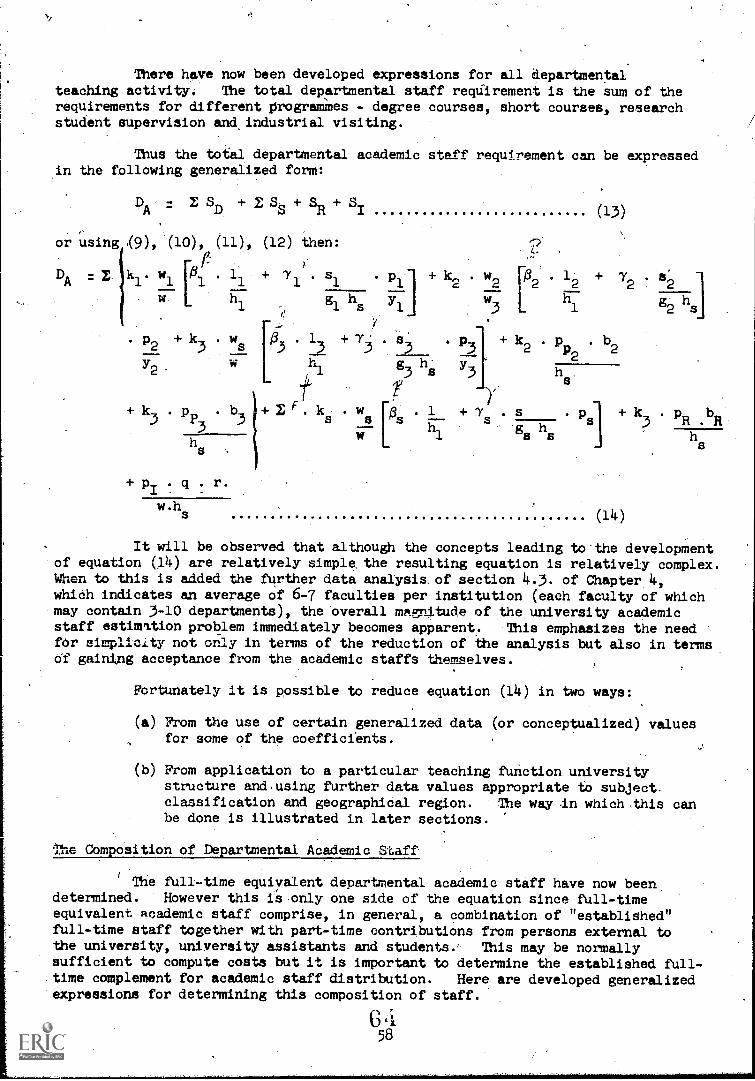
There have now been developed expressions for all departmentalteaching activity. The total departmental staff reqUirement is the sum of therequirements for different programmes - degree courses, short courses, researchstudent supervision and, industrial visiting.

Thus the total departmental academic staff requirement can be expressedthe following generalized form:

DA. I SD

+ Z S. + + S-S R I (13)

Or Using ,(9), (10), (11), (12) then:

..f;DA : Z k,. w, r., . 11 + 71 .

1g1hs

:11 k2 ww;

12 + 72

h1 g2 lid

i ....2... i

w h

P2 + k3 ws 135 12

Y2. Lh

PI ! q : r.

w.hs

+ .7.

.ws

w

3. p

3y

+ 7r

s

+ k2

.

. s

pp

.

2

b2

g h-3 8

1'0s . 1

--h1

hs

ps + k3gs hs

(14)

. pR .bR

h8

It will be observed that although the concepts' leading to the developmentof equation (14) are relatively simple, the resulting equation is relatively complex.When to this is added the further data analysis. of section 4.3. of Chapter 4,whiCh indicates an average of 6-7 faculties per institution (each faculty of whichmay contain 3-10 departments), the overall maanitude of the university academicstaff estimItion problem immediately becomes apparent. This emphasizes the needfor simplicity not only in terms of the reduction of the analysis but also in termsOf gaining acceptance from the academic staffs themselves.

Fortunately it is possible to reduce equation (14) in two ways:

(a) From the use of certain generalized data (or conceptualized) valuesfor some of the coefficients.

(b) From application to a particular teaching function universitystructure and -using further data values appropriate to subject.classification and geographidal region. The way in which,this canbe done is illustrated in later sections.

The Composition of Departmental Academic Staff

The full-time equivalent departmental academic staff have now beendetermined. However this is only one side of the equation since full-timeequivalent academic staff comprise, in general, a combination of "established"full-time staff together with part-time contributions from persons external tothe university, university assistants and students.' This may be normallysufficient to compute costs but it is important to determine the established full-.time complement for academic staff distribution. Here, are develOped generalizedexpressions for determining this composition of staff.

(34.

58

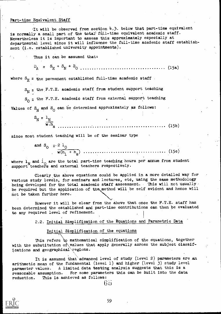
Part-time Equivalent Staff

It will be observed from section 4.3. below that part-time equivalent

is normally a small part of the totaf fall-time equivalent academic staff.

Nevertheless it is important to assess this approximately especially atdepartmental level since it will influence the full-time academic staff establish-

ment (i.e. established university appointments).

Thus it can be assumed that:

D - S+S+ SA E N 0

where SE the permanent established full-time academic staff ,

SN the.F.T.E. academic staff from student support teaching

So the F.T.E. academic staff from external support teaching

Values of SN

and S0

can be determined approximately as follows:

S - 1N N

w.hs

since most student teaching will be of the seminar type

(15a)

(15b)

and S --2 10

w(h1 + hs) (15c)

where 1 and 10 are the total part-time teaching hours per annum from studentsupport teachers and external teachers respectively.

Clearly the above equations could be applied in a more detailed way forvarious study levels, for seminars and lectures, etc, using the same methodologybeing developed for the total academic staff assessment. This will not usually,

be required but the application of th method will be self evident and hence will

not be taken further here.

However it will be clear from the above that once the F.T.E. staff hasbeen determined the established and part-time contributions can then be evaluated

to any required level of refinement.

2.2. Initial Simplification of the Equations and Parametric Data

Initial Si lification of the equations

This refers b mathematical simplification of the equations, together

with the substitution o values that apply generally across the subject classif-

ications and geographical ,egions:

It is assumed that advanced level of study (level 2) parameters are an

arithmetic mean of the fundamental (level 1) and higher (level 3) study level

parameter valueS. A limited data testing analysis suggests that this is a

reasonable assumption. For some parameters this can be built into the data

reduction. This is.achieved as follows:

G ii

59

(i) Insertion of:values for k. These, are, effectively, factors foracademic staff teaching loads at the various levels of study. Thussince hi and h are referred to at the fundamental level, k1 1generally. . ATso a limited amount of data testing suggested a valueof k .7. 1.5 (with kl = 1). This value leads to an overall studentweigting of higher to first degree/diploma work of between 2.0and 2.5, which is approximately the value quoted nationally andinternationally. Appendix Al gives an analysis which supports thisconclusion.

Thus k1

= 1.0 k2

= 1.25 k3

= 1.50

(ii) Insertion of values for b. These relate to academic staff''supervision of project/theses and student research. A brief analysisof typical values is given in section 3, Chapter 4, where it is 7'suggested that values of b are relatively uniform across subjectclassifications and geographical' regions although medicine appears tobe between two and three times greater than for all other subjects.Appropriate values for b are:

b2

- 0.5 b3

- 0.75 bR

- 1.20

(iii) The assumption that advanced level parameters are an arithmetic meanof the fundamental and higher level parameters is applied to theparameters 1 and s

h1

i.hs

Let 13 = u.11 s3 v. slg. gl

A

Then 12 (

1 + 11

2 .41.2 - 1+vs

i 2- ( 2 ) 1

gl (16)

Use of all of the above simplifications in the basic programme of studyequation (4) leads to:

Sy 11 . wi 0.625 (1 + u)w2 1.5u. w3 s1

wl . pi + 0.625 w2 . p2+ +

h1

w w w gl hs w yl w y2

(1 + v) + 1.5 w3 . p3 . v

w y3

+ 1 [0.625 p +1.125 p ]Tis-

- P2 P3(16)

This is now in a form which provides considerable simplification whenapplied to a specific programme of study structure. This is illustrated byapplying it to the same examples as in section 2.1.2. as follows:

.._ First Degree in the U.K.

level.This incorporates 2 years at the fundamental level and 1 year at advanced

6o

Typical values are:

w w21 = 2

Y1- 1

Y21.

together with the above parameter values, this yields:,

Sb 11 [2.625 + 0.625 u] +si [pi + 0.625 p2 (1 v)] + 0.625 Pp2

h1 g1oh

shs

Higher (Masters) Degree ih the U.K., by Course

w3 2 Y _ - r)

3. (all others zero).

w 3

Sb 11 . u si

Y 17. v . p

3+ 1.125 p

3g . h

sh

First Diploma in a Ehropean University

This normally embraces 3 years at fundamental level and 2 years at

advanced.

'Typinn.1 values would be:

w1 :,.. 3 Y

w2

1 = 3 7. 2 y,, 2 (all, higher level zero).

Y 1

11 [4 + ul + s1 + 0.625 p2 (i + v)] + 0.625 pp

1gl hs hs

The evaluation of the specific instances sited above depends on aknowledge of the parameters 1/h1, s/g.hs, u, v, and hs for any given studentenrolment in .a programme of study. These parameters will in general vary with

subject area and geographical region.

It will be obvious from the above that a similar simplificationprocedure can be adopted for the departmental contributions expressed by equation(14). However to avoid confusion from repetition of generalized equations atten-tion will now be directed to the application.of the methodology to a particulargeographical region. Before this,"it is necessary to present the_results of adata analysis for the value's of the controlling parameters in the equations andthis follows in the next section.

Parametric Data

The data collected from reference 1 has been reduced to provide values

of l/h1,

s/g.h6'

hsl

u and v in terms of broad subject classification andgeographical region.

Some details of this are given in section 3. of Chapter 4 and theresults are presented here in a form for immediate application to the derivedequations. Basically they present standard values of the parameters for six broadsubject classifications together with geographical region weighting factors for

four regions. The data is presented'in tables 12 and 13 below.

61

Table 12. Parametric Data ftor Subject Classification

Subject classification1l/h

1

sl/gl'hs

u v hs*

Pure Science 1.18 0.0525 0.636 2.100

echnology/Applied Science 1.44 0.0513 0.778 1.780

ledical Science 1.78 0.0602 0.669 1.292

1 manities and Art 1.13 0.0281 0-752 1.887

.ucation 0.96 0.0283 0.760 1.629

ocial Science/Law 1.56 0.0250 0.744 1.652

.11 Subjects 1.32 0.0423 0.747 1.491 11.58

* Only the overall value is quoted here as this is recommended for use with theproject/thesis/research supervision terms of the equations.

Table 13. Geographical Region Weighting Factors,

Factor Applied

---Z....7---Region

,

sl/g

1.h

s

u v,

hs

rorth America 0.84 0.86 0.82 1.14 1.08

nited Kingdom 0.69 1.40 1.19 1.21 1.00

I rope: EEC and Scandinavia 0.91 0.79 1.15 0.99 0.98

1 rope: Others 1.79 1.26 0.99 0.80 0.77

Example of use: The value of v in Humanities for Europe (others) is 1.887 0.801.5L

This table may be used to select appropriate data for substitution in theacademic staff equations. It is particularly useful for comparative purposes.The similarity of some of the parameters suggests that further simplications mightbe made with a small loss inaccuracy (e.g. grouping Science and Technology on theone hand and Human Ries, Education and Social. Science on the other). This howevernas not been tested.

/ 62

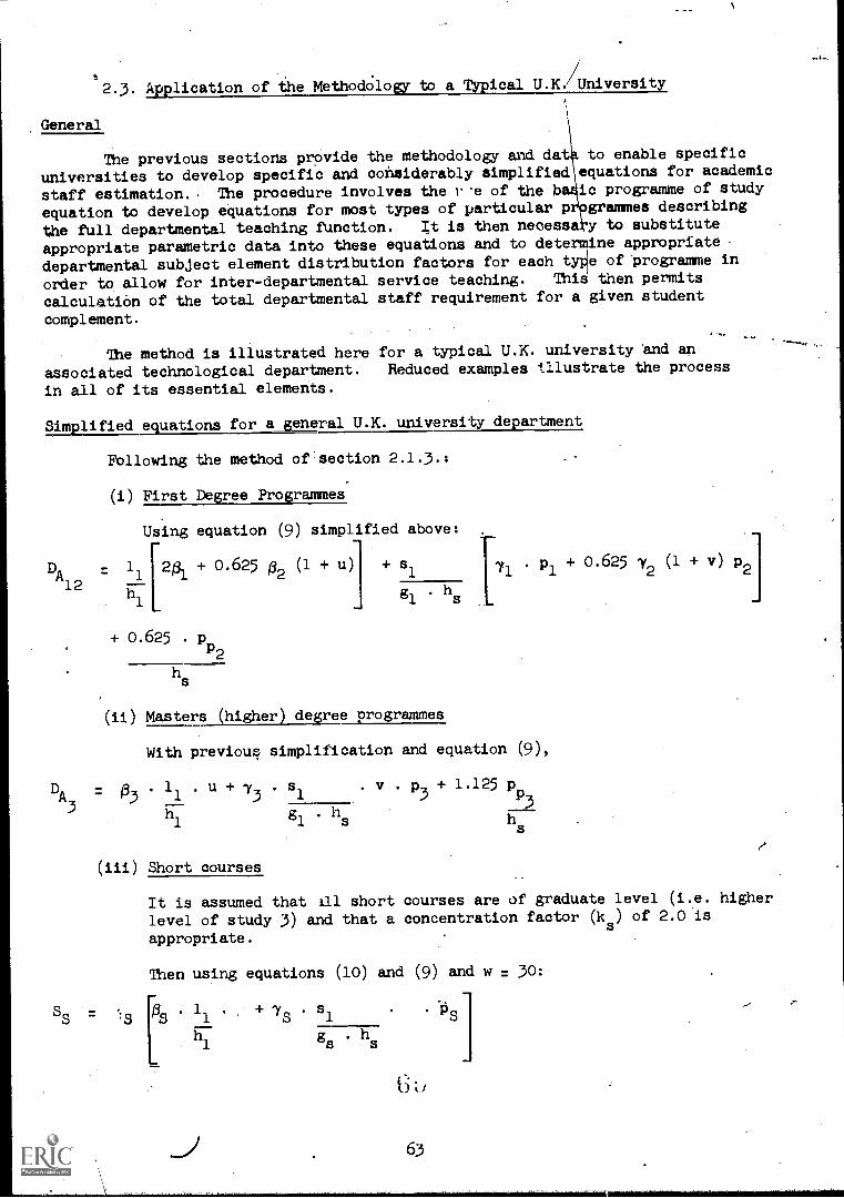
t

2.3. Application of the MethodOlogy to a_Dpical U.K.' University

General

The previous sections prOvide the methodology and da to enable specific

universities to develop specific and considerably simplified equations for academic

staff estimation. The procedure involves the re of the b is programme of study

equation to develop equations for most types of particular p grammes describing

the full departmental teaching function. It is then necessa y to substitute

appropriate parametric data into these equations and to determine appropriate

departmental subject element distribution factors for each tylie of 'programme in

order to allow for inter-departmental service teaching. This then permits

calculation of the total departmental staff requirement for a given student

complement.

The method is illustrated here for a typical U.K. university and an

associated technological department. Reduced examples tilustrate the process

in all of its essential elements.

Simplified equations for a general U.K. university department

Following the method of section 2.1.3.:

(1) First Degree Programmes

Using equation (9) simplified above:

DA = 11 201 + 0.625 02 (1 + u) + si 71 . pl + 0.625 72 (1 + v) p2

12 h1 gl hs

+ 0.625 . p

P2hs

(ii) Masters (higher) degree programmes

With previout simplification and equation (9),

DA i 03 . 11 . u + 73 . si . v . p3+ 1.125 pp

3 h1 gl hs h

3

s

(iii) Short courses

It is assumed that ill short courses are of graduate level (i.e. higher

level of study 3) and that a concentration factor (ks) of 2.0 is

appropriate.

Then using equations (10) and (9) and w = 30:

Ss -]=

[

Os . 11 . + 7s . siPS

h1

g hs s

U

63

(iv) Research Supervision

Using (12):

SR.= 1.8 p

Rh

(v) Industrial Visiting

Using (13) and w 30

SI= 0.4 r . pI

hs

The summation of the requirements for these functions of the departmentalacademic staff yeilds the academic staff complement required by the department.

Algebraically:

= 1,

i

201 + 0.625 02 (1 + u) + si 71 pl + 0.625 72 (i + v) p2

h g1

.,hs

+ 0.625 . pP2

hs First degree programmes

+ E, ez 1 . u + 73 . sl., 1

[

v.p3

+ 1.125

. 0s

/

pP

hs

+ 1.8

Research

Masters degree programmes

pR + 0.4 r.p,

h g11

+ws 0S

11

u+ 7S

[ h1

Short courses

.

s1

hs

v

gs

. hs

hs

hs ,

Industrialsupervision supervision

A2plIpstion to a Specific Technology Depatment

Using tables 12 and 13 from section 2.2. the following data is appropriateto a technology department in a U.K. university

111.44 . 0.69 = 0.994

hl

0.0513 . 1.4 = 0.0719. hs

0,778 . 1,19 = 0.927

v = 1.760 . 1.21 3. 2.17

064

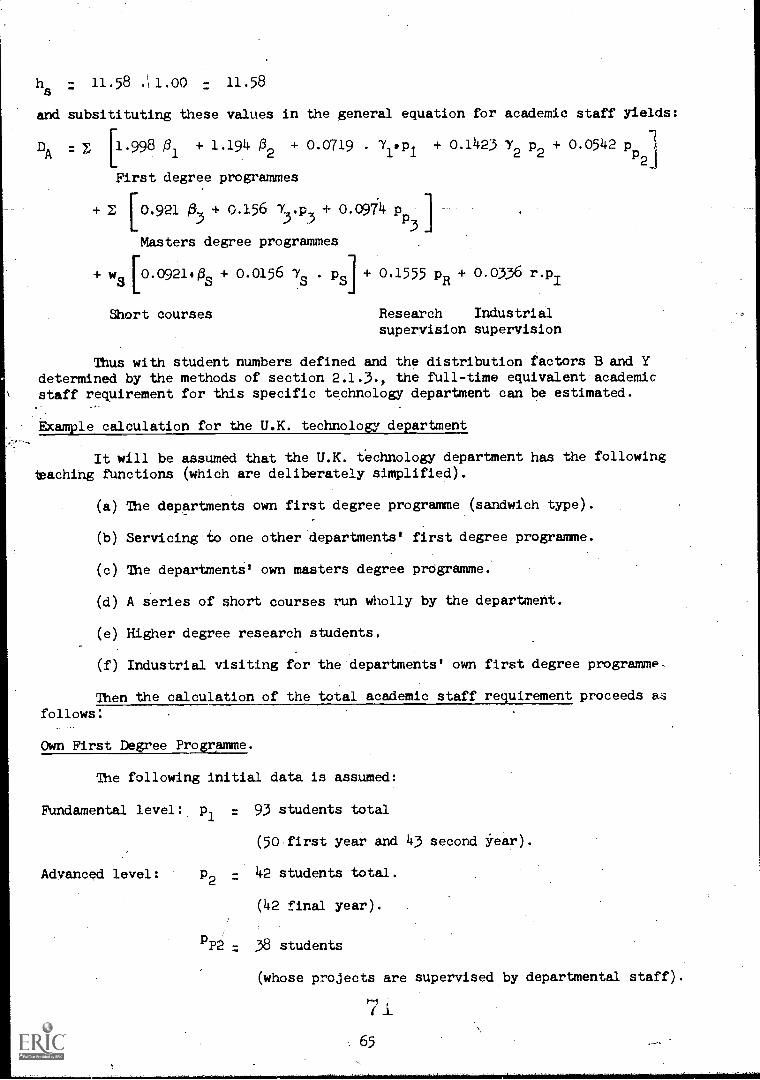
hs

- 11.58 .1.00 ...: 11.58

and subsitituting these values in the general equation for academic staff yields:

[DA : 72, 1.998 01 + 1.194 02 + 0.0719 . 71.pi + 0.1423 72 p2 + 0.0542 p

P2 1

First degree programmes

+ Z [ 0.921 03+ 0.156 7

3.p3+ 0.0974 pp

Masters degree programmes

+ ws [0.0921.5 + 0.0156 7s . pal + 0.1555 pR + 0.0336 r.pI

Short courses Research Industrialsupervision supervision

Thus with student numbers defined and the distribution factors B and Ydetermined by the methods of section 2.1.3., the full-time equivalent academicstaff requirement for this specific technology department can be estimated.

Example calculation for the U.K. technolottydepartit

It will be assumed that the U.K. technology department has the followingleaching functions (which are deliberately simplified).

(a) The departments own first degree programme (sandwich type).

(b) Servicing to one other departments' first degree programme.

(c) The departments' own masters degree prOgramme.

(d) A series of short courses run wholly by the department.

(e) Higher degree research students.

(f) Industrial visiting for the departments' own first degree programme,

Then the calculation of the total academic staff requirement proceeds asfollows:

Own First Degree Programme.

The following initial data is assumed:

Fundamental level: pl = 93 students total

(50 first year and 43 second year).

Advanced level: p2 42 students total.

(42 final year).

P 38 students

(whose projects are supervised by departmental staff).

65

Then it is first necessary to calculate the distribution/tactors for thecomplete programme of study according to the methods outlined section 2.1.3.This is effected in the following tables 14 and 15 for the fu damental andadvanced levels respectively.

Before proceeding to the calculations it is useful/4.o comment on theresults of tables 14 and 15. These are.: ///

(0-The overall value of 0 for the of the programme(table 14) is considerably less than unit because.common lecturingprovides a greater weighting than the repetition of lectures (seecolumns "x' and "c") .

Conversely for the advanced part the value of 0 is greater than unity.

(ii) The overall value of y is unity for bOth parts of the programme (as itshould be).

.(iii) The department's own contribution, shown in the subject distributionfactors 01 and 7

1,is relatively small at the fundamental level, and

considerably greater at the advanced level.

(iv) The summations for 0 and 7, excluding Oand present thedistribution factor crediting tose41.)Eirtments servicing the programme.Hence of the total staff required for the programme -at fundamental level,the mathematics department is credited with 6.58/.6339 per cent ofthem for lectures, and 13-52% for classes.

(v) It will be noted that no allowance is made for project/thesis work asthis is accounted for separately.

(vi) All elective subjects are included - this is especially significantin the advanced part of the programme.

Thus the department's own academic staff requirements to provide itsundr6raduate degree course, can be calculated via tables 14 and 15, fromoluattt:m 9.

01

71

1

-

=

0,3684

0.5045

95

0c

72

p22

= 0.8334

- 0.7916

- 42 pp2

- 38-

F,)r first degree programme:

DA 1.)2J8.01+1.194324-0.0719 71 pl + 0.1423 72

p2

+ 0.0542 pP2A

2.5,

1.928. 0.5684 + 1.194. 0.8334 + 0.0719. 0.5045. 93 + 0.1423. 0.7916. 42

+ 0.0542. 38

11.891

i.e. 11.89i full-time equivalent academic staff are required by the technologydepartment to teach its own undergraduate programme in aeronautical engineering.

66

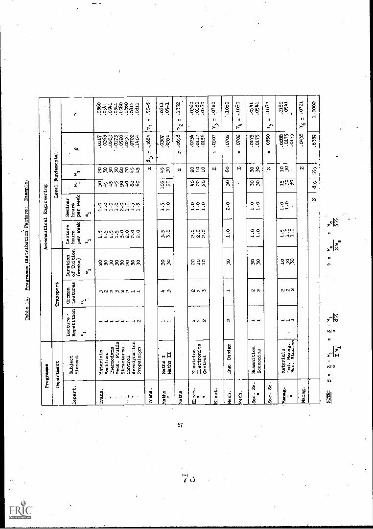
Table 14.

Programme Distribution Factors:

Example.

Programme

Aeronautical Engineering

Department

Transport

Level Fundamental

Depart.

Subject

Element

Lecture

Repetition

xi

Common

Lectures

Cl

Duration

of Tuition

(Meeks)

Lecture

hours

per week

Seminar

hours

per week

w 1ws

07

W1

11

81

Trans.

Materials

13

20

1.5

1.0

30

20

.0117

.0360

nMachines

12

30

1.5

1.0

45

30

.0263

.0541

nThermodyns

1'

230

1.5

1.0

45

30

.0263

.0541

nMech. Fluids

13

30

1.5

1.0

45

30

.0175

.0541

9Structures

12

30

3.0

2.0

90

6o

.0526

.1c60

If

Control

12

20

2.0

1.0

40

20

,0234

.0360

IfAerodynamics

11

30

2.0

1.5

6o

45

.0702

.0811

IfPropulsion

21

30

2.0

1.5

6o

45

.1404

.0811

Trans.

zt3,

-.3684

7- .5045

II I

1

Maths

Maths I

14

3o

3.5

1.5

105

45

r

.0307

.0611

Maths II

3.

330

3.0

1.0

90

30

.0351

.0541

Maths

iI

= .0658

72

: .1352

Elect.

Electrlcs

12

20

2.0

1.0

40

20

.0234

.0360

Electronics

12

10

2.0

1.0

20

10

.0117

.0180

nControl

23

10

2.0

1.0

20

10

.0156

.0180

Elect.

M= .0507

70720

Mech.

g. Design

21

1I

30

1.0

2.0

I30

1 '60

.0702

.1080

mech.

M= .0702

7- -10819

Soc. Sc.

Humanities

12

30

1.0

1.0

30

30

.0175

.0541

Economics

12

30

1.0

1.0

30

30

.0175

.0541

Soc. Sc.

Ee '.0350

75- .1082

Manag.

Materials

12

10

1.5

1.0

15

10

..0088

.0180

Ind. Manag.

,1

230

1.0

1.0

30

30

.0175

.0541

nElls. Studies

12

30

1.0

-30

-.0175

-

Manag.

M.0438

76

: .0721

1855

555

.6339

1.0000

NOTE:

=x

. wi

c

wl

=X

wl 67

7 =

ws

555

-wa

Table 15.

Programme Distribution Factori

Programme

Aeronautical Engineering.

Department

Transport

Level

Advanced

Depart.

Sub ject

Lecture

Repetition

Common

Lecture

Duration

weeks

Lecture

hrs. /week

Seminar

hrs./Week

--

Element

xi

ci

wi

1i

Si

wl

ws

07

Trans.

Aerodynamics

11

30

21

60

30

.1429

.1250

if

Structures

12

30

21

60

30

.0714

.1250

le

Propulsion

2-

130

21

60

30

.2858

.1250

It

Stability

12

30

21

6o

3o

.0714

.1250

uDesign

11

30

21

60

30

.1429

.1250

uDesign Tbpics

12

20

120

20

.0238

.0833

iii

Synthesis

11

20

21

40

20

.0952

0833

1

l02

: -8334

.7916

Ergon.

Design Topics

12

10

110

10

.0119

.0417

Z.0119

.0417

Maths.

Maths. III

210

21

20

10

.0952

.0417

Y.0952

.0417

Soc. Sc.

Econ. and Soc.

130

11

30

30

.0714

.1250

-

Z.0714

.1250

Z420 1240

1.019

1.000

NOTE:

0 =

x. wl

-x . wl

c2wl

cJ5

7ws

=ws

Zws

24-5

Servicing to other departments' programme.

Here it will be assumed that servicing is to the advanced level of another

technological programme and for which:

i'. .

02 = 0.1i

05 -.., 7 - 0.087 P2= 6o 'la

P:...- 4

2t 2

(also: 0 - 7 - 0)1

The general simplified equation is again utilized:

DA

= 1.194 . 0.105 + 0.1423. 0.087. 6o 0.0542. 4

121.085

i.e. 1.085 F.T.E. academic staff are required by this technology department to

service the outside technological programme.

Own masters degree prograrr-,-,

To avoid unnesessary complication full distribution factor tables similar

to tables 14 and 15 will not be reproduced here. Thus it will be assumed that:

0 0.700 7 -- _ _ 0.750 p3 = 20 p

P= 15

3Master's degree requirements for academic staff are:

DA3

[0.921. ij3

+ 0.156 7 p + 0.0974 p3 P

3

al0.921. 0.700 + 0.156. 0.750. 20 + 0.0974. 15

4.446

The master's degree programme in technology necessitates the technologydepartment having 4.446 full-time equivalent academic staff.

Short course programmes

Here it is assumed that 12 weeks (total) of short courses are givenentirely by the departmental staff with an average of 18 students per course i.e.

ws 2 12 0 7 - 18.S S =

1 PS

The relevant calculation is:

Ss = ws [0.0921.0s + 0.0156 7s. Ps]

-.1. 12 [0.0921 + 0.0156.18]

..: 4.475

The transport department's short courses require 4.475 full-time equivalentacademic staff to teach them alone.

Research supervision

It is assumed that there are 15 full-time research students requiring

supervision: i.e. pR = 15.I*?

69

The relevant calculation from equation (37) is:

SR

0.1555 pR

0.1555 . 15

2.333

Research student supervision requires 2.333 full-time equivalent academic staff-within-the technology department.

Industrial visiting etc.

Since the first degree programme is of the sandwich type it is assumed thatall students are in industry for 1 year between the fundamental and advancedlevel studies. It is also assumed that each student is visited twice duringthis annual period i.e.:

pI

43 r s 2

The relevant calculation is:

- 0.0336 : r. pSI

= 0.0336. 2. 43

= 2.890

The total academic staff requirement, in full-time equivalents, for thistechnology department is summarized in the following table 16:

Table 16. Total F.T.E. Academic Staff Requirement

- Transport Department: Example.

ItemOwn 1stDegreeProg.

Servicingother 1stDegreeProg.

OwnMastersDegree

Prog.

ShortCourses

ResearchSuper-vision

Indust.VisitingEtc.

Tbtal

AcademicStaffRequir. I. 11.891 1.085 4.1146 4.475 2.333 2.890 27.120

%. off

Total 43.8 4.0 16.4 16.5 8.6 10.7 100.0

3. Estimation of Departmental Technical Support Staff

1/The estimation of departmental supporting staff is important in that it

contributes significantly to the total recurrent costs of a department particularlyin the science and technology areas where considerable laboratory and other supportspace is involved. However it is equally important to academic staff if they areto perform their duties effectively and efficiently. The latter applies whetherthe supporting staff is large or small in relation to the total academic staff.

I ti

70

For example the arts, social sciences and humanities require adequate supporteven though this will not be on the scale of that required for, say, engineering.

This section, therefore, presents a simplified method of estimating suchsupporting staff for departments. This staff refers not only to technician staffusually associated with science and technology but also to assisting staff for

any academic purpose (but excluding administrative staff).

The method supposes that supporting staff is a function of departmentalsuppOrt area and of the total departmental academic staff support area in thiscontext includes working spice of all kinds, necessary to the adequate functioning

of the department. A large portion of this may be laboratories. However arts,

social science, etc. departments also need such space although it will be smallgenerally compared with laboratory-based science and technology. The data

analysis (reference 4) shows this to be so.

The method. proceeds initially to test the basic suppositions in terms ofsupport area using the full data from reference 1 and then proceeds to developan expression for support area in terms of academic staff. The final resulttherefore is presented as a function of academic staff which can be calculated

from section 2 and of data derived constants.

The data suggests that departmental supporting staff is much less sensitiveto geographical regional variations than to broad subject classification so thatthe data constants are presented in terms of variation of the latter only.

It will be observed that a by-product of the method-is-an analysis whichfacilitates the calculation of departmental support area in terms of departmental

academic staff.

3.1..Basic Methodology

A preliminary study of the full data of reference 1 suggested that the-departmental supporting staff was largely dependent-on departmental support area

and total academic' staff. It further suggested that the data could be grouped

into the following broad subject classifications:

Group 1

Group 2

Group 3*

Group 4

Pure Science

Applied Science and Technology

Arts/Social Science/Law/Mathematics/Education

Medical Sciences

*' That mathematics is included in Group 3 and that geographical regionalvariations were relatiVely small.

Appendix A2 of this chapter tests these observations. The results shows.reasonably good linearity between support area and supporting staff for each group.The proportionality is less good between total academic staff and supporting staff.This was subsequently shown to be the minor influence and averaged constantproportlonalities were assumed for each group.

Thus Ab- d

3'from the graphs of Appendix A2

"T

NT

(17)

Where Ab = departmental support area (m2)

NT = total departmental support staff (excluding administrative)

also N -T (18)ST

where ST = total departmental academic staff.

Thus if:, NT = d1 . Ab + d2 . ST(19)

then Appendix A2 derives values of d1 and d2 from d3 and d4 (using. group 3 data asa base as follows:

NT d1 Ab + 0.07 ST

-1 b T (20)

Table 17 presents the values of d1,

d2, d3

and d4.

Table 17. Values of Proportions d d2, d3, d4.

Subject Classifications d1 d2

d3

Group 1. Pure Science 0.00855 - 105 0.68

Group 2. Applied Science and Technology 0.00647 ' - 139 0.69

Group 3. Arts/Social Science/Law/Maths/Education o.oc444 77 0.106

Group 4. Medical Sciences 0.00892 - 99 0.60

\ Average 0.07

Thus for a given "support" area and academic staff, the departmentalsupporting staff can be calculated for any subject clabsification group.

However departmental "support" area is itself related to academic staff.If this relationship can be specified, supporting technical staff can be calculateddirectly from academic staff.

The estimation of departmental "support" ("laboratory") area.

The method for the determination of departmental support'area distributionfactors in terms of academic staff, drawn from reference.2, is as follows:

Let: S = total departmental academic staff required for higher degree/diplomaresearch and other higher level of study work. (This can bedetermined from section 2).

ap r. support area per first degree/diploma student (m2)

= ratio of higher degree/diploma support area per student to ap

factor to allow for different types of support work.

72

su

Is overall university student/staff ratio (calculated using section 2

of this chapter by departmental aggregation).

Then the "effective" number of staff in a department is:

For first degree/diploma = su (DA)For higher degree/diploma su . SH

Hence Ab : 0 [su(DA - SH) al + su . DA . co . ap 1 .

or Ab

su 0 ap (DA - SH) +w.SH(21)

Values a and w are data derived in Appendix A2 and equation (21) can be

rewritten assF

Ab

- su

r 6.1 ( - SH) + w SH(22)

where r . ox2 , and is the "effective" value of 0, which varies according to

subject area of the department, conditioned by the group factor .

3.2. Departmental Support Staff Estimation.

If we substitute equation (22), expressing total support area in terms of

academic staff, into equation (20).

Ds d1 su r . 6.1 [(DA - SH) + w SH] + 0.07 DA

Thus su'

DA

and SH can be determined from section 2 and the values of d1

and w are given in tables 7 and 8 respectively.'` It remains to determinesuitable values of . Appendix A2 gives a method for determining this from the

data of reference 1. However the results are somewhat varied for individualdepartments due, probably, to the unreliability of the data at this level of

disaggregation. Nevertheless they are of the right order of magnitude and somevalues 'compare well with those used in a U.K. university (see Appendix A2).

In the absence of more reliable data the following broad subject classifi-cation values for r may be used as a guide (table 18):

Table 18. Data-Derived Values of w and r .

Subject Group Subject w r

Group 1 Pure Sciences 2.26. 0.72

Group 2 Technology 2.18 1.04

Architecture 0.30

-Agriculture 0.95

Group 3_ Fine Arts 2.80 0.05

Social Science 0.15

Law 0.01

Humanities 0.03

Education 0.14

Group 4 Medical Sciences 2.26 1.20

73

It should perhaps be added that very little published information existsfor the determination of "support" area coefficients for specific subjects astypified by r and that this is a field requiring research.

3.3. Example Applied to the Typical Technology Department in the U.K.

Based on the previous example of the technology department in the UnitedKingdom, detailed in section 2.3:

Total departmental academic staff DA : 27,12

Total departmental academic staff required for all higher level work:

SH 4,446 t 4.475 + 2.333 = 11.254

Frail table 17:

- 4,047 for group 2.

From table 8;

; 2,18. tor grouP 2

r = 1.04 ficoNteohnology.

Since the calculation tiksecttork 2.3. did not proceed to the eggregateiuniversity situation it 1,4 necaseaV* to assume a typical value for the overall,staff/student ratio (au), Thus fOle tYpical university:

su = 9'5

Then from equation (22):.

"support" area Ab 9.5 1.04

= 2435 m2

. 1 [(27.12 - 11.25) + 2.18. 11.25]

and from (20);

0.00647 2435 + 0.07. 27.12 = 17.65

"Support" area (including laboratories) for this department is 2435 m2, and17.65 full-time equixalant technical support staff are required.

4. Estimation of Departmental Administrative Staff

4.1. Basic Methodology

Since the method of calculation of departmental academic staff (section 2)and of supporting staff, other than administrative staff, (section 3) effectivelydefines the academic function and type of the department it is logical topostulate that the number of departmental administrative staff is a function ofthe'total departmental academic and supporting staff. Furthermore it is areasonable assumption that administrative servicing would relate to the degreeof responsibility of such other staff. These are the bases of the simpleanalysis that follows.

(.j U

74

Let -T

total full-time academic staff in a department

DD

- total full-time administrative staff in a department

DS

- total full-time supporting staff (technicians, assistants,demonstrators, etc.) in .a department but excluding administrative

staff.

A4suming that academic staff can be classified into three broad gradidgH

1. Professoral: xl = factor of academic staff (DA)

2. Senior: x2 .7 factor of academic staff (DA)

3. Junior: x - factor of academic staff (DA)

at grade 1.

at grade 2.

at grade 3.

where x1

+ x2

+ x3

- 17

Then the proportionate administrative staff support can be expressed as:

1administrative staff per grade 1 academic p taff

2administrative staff per grade 2 academia staff

3administrative staff per grade 3 accede

Tadministrativestaff-per. supporting

and will be ordered in decreastngyialues of

Thus the total departmental administrative staff required is:

is staff

aff (Ds)

( 1 xl 2 x2 x3) IPA

This can be written as:

DD

= n. E A +T

or DD= n +

DA

where n =

T. D

SDA

1 xl 2 Pc2 3 x3'

(23a)

(23b)

(23c)

These data cover 323 individual items and the values of table 9 are plotted

in graph 1. This plot shows that there is little evidence of subject dependencyexcept that the humanities/arts/social science type subjects bunch towards the

D ordinate since the supporting staff is small in these areas. It alsoD/DA

shows a good degree of linearity and hence justifies the assumptions of equation

(23)-

A good expression from the straight line of graph 1 is:

DD : 0.178 DA + 0.085 Ds

8

75

(24)

Equation (23) can be tested using computerized departmental data fromreference 1 and the results are summarized in table 19:

Table 19. Pro ortions of Administrative and Technical Staff to

Academic Staff by Department

Department*DD/D

A Department* ADS /DA

Pure Sciences

0.245

0.195

0.269

0.229

0.220

0.885

0.694

0.472

0.387

0.410

Agriculture

0.895

1.360

04. Biology

06. Chemistry

08. Geology

10. Maths

13. Physios

41/43. Agric.-exid. Fbr stry

44. Vet. Medicine

0.264

0.302

Humanities

t

,daq5

0.0*

0.04

0.026

52. History

53. Languages

56. Philosophy

58. Theology

0.162

0.162

0.129

0.186

Architecture

.0.204 0.20419. ArChitecture

Technology

0.252

0.208

0.185

0.237

0.204

0.205

0.824

0.332

0.717

0.546

0.554

0.653

Fine Arts

0.061E20. Eng. Science

21. Const. and Civil Eng.

25. Ind. and Prod. Eng.

26. Elect. Eng.

27. Mechanical Eng.

28. Chem. Eng.

61A4:. All kinds, ,0.190\

E on

0.03765. Flucation 0.214

Law

0.07110. Law 0.226

Medical Sciences

0.286

0.190

0.167

0.606

0.513

0.679

Social Sciences

0.098

0.040

0.198

0.039

31. Dentistry

32. Medicine

34. Pharmacy

71. Business & Committee

72. Economics

73. Geography

78. Sociology

0.253

0.179

0.168

0.228

Overall Average 0.213/

0.411

* The number reference refers to the computer coding.

76

Aa

6).3

e

TH

EO

L.B

AR

T

g6E

04Lk

-

LAN

ct)

0/4/

s0

0

Bus

/com

mE

ecE

SoC

. 00 LA

P1

o

MA

TH

S. 0

CI V

IZ.

E.A

I

0ae

oL.

FIG

UR

E 1

EA

/4.

AG

R/c

/Fb

RE

sT.

0 0 if

o 4

..0

Eac

r

--- P

ritt.

DD

= 0

178

7,-.

0-0g

.rD

3

DA

-

A t

CN

EK

EA

V.

00

CH

EM

.

IWO

/PR

OP

EA

/4

6.r

AP

*R

ELA

T/a

NS

HIP

56-

7-w

EE

A/

-X14

1DE

Aftc

AA

ID 5

UP

PaE

TiN

c_i

_.5-

T4F

F_L

AN

D 4

cvv

/sA

//57R

A T

i VE

--S

TA

PP

AT

DE

PA

RT

ME

NT

AL

E V

E-L

;

VE

T

Me)

.1.

3o 1

()

)1

0 -I

- 2.

a-3

ogo.

504

:,o7

a$_

ecal

o of

5aP

AD

RT

/Ale

; ST

AF

F -

-fir;

=71

-c41

)-E

714r

.-c

DS

/DA

which indicates a bias towards academic staff for administrative support, aswould be anticipated. Administrative staff numbers are now rapidly determinablefrom acuiemic and technical support staff.

It should be noted that once equation (23) has been evaluated departmentallyit can be summed to give the total university departmental administrative staff andthis together with the information of section 4.3. of Chapter 4 can then provide anapproximate assessment of additional central administration staff required. (Itis about 40+50% of the university total).

4.2. Application of the Method to the U.K. Universities

Although it is possible to apply the simplified equations directly, toprovide a more accurate figu're for administrative staff of particular departments,it is necessary to investigate the relationships between administrative staff andvarious grades of academic staff applicable to those departments. Once deter-mined, such values can be used in equation (23) for any given composition ofacademic staff (any values of x.

'x2

and x3).

For the U.K. the following approximate value/s of x are generally admittedby the University Grants Committee.

Professors: x1

- 0.125

Readers, Senior Lecturers: x2

- D.225

Lecturers: x3

= - 0.650

.(Research fellows funded by the university would normally be included in anappropriate catagory).

As an initial assumption for the values of , let1

x1 : x2, : x1 2' 3

: 1 : 1

1 2 3

(which may be regarded as a "responsibility" equation.

Men: x1

1

x1+ x

2.+ x

3 1 1+ +

1 2 3

but x1+ x

2+ x

3= - 1.

1,et 1 x1 1

- ( 1 + 1 + 1 ) x2 2_ _

1 2 3

etc.

Thus 1/

using the values from the initial simplification, then:

1 = 0.0593 and . 0.085

= 0.0475 , is 0.264 = 0.092

CP4

78

3 (57)

These represent 2.11 Grade 1 academic staff to 1 administrative staff

3.79 Grade 2 academic staff to 1 administrative staff

10.9d Grade 3 academic staff to 1 administrative staff

11.80 support staff to 1 administrative staff, and providereasonable guide values. Thus, using these, equation (23) becomes:

DD - (0.475 x1

+ 0.264 x2

+ 0.092 x3) DA

+ 0.085 DSS

for any academic and supporting staff composition.

Example calculation applied to a typical U.K. technology department

From UGC data: xi = 0.125, x2 = 0.225, x3 = 0.650

From table 6 of section 2.3: S = 27.12

From section 3.3: Ds 17.65

Thus DD = (0.475 . 0.125 + 0.264 . 0.225 + 0.092 . 0.650) 27.12 + 0.085 . 17.65

or 6.33

i.e. the technology department described above requires 6.33 full-time departmentaladministrative staff.

Appendix Al

Weighting of Fundamental to Advanced Levels of Students in Relation to

the Value of k3.

A short analysis relating to U.K. universities was undertaken to investigatethe suitability of a value of k

3- 1.5 in the academic staff equation of section 2.2.

Using the geographical region weighting factors of table 13 section 2.2. forU.K. universities and the simplified first and higher degree equations of,the samesection, with:

P - P2 P andP2 1

2 P-

33

P1

;1.14 P2

+ 1.03 P2

- 2.17 P2

(i.e. 14% and,3% wastage in the 1st and second years respectively).

Then:

Sy12 - 1 + 0.513 u) + P2

s1

(3.91 + 1.06 v) + 0.0542

hl g1

. hs

- Go

+ dIo . P2 A1.1

where Go

11

(1.81 + 0.513 u)

hl

8679

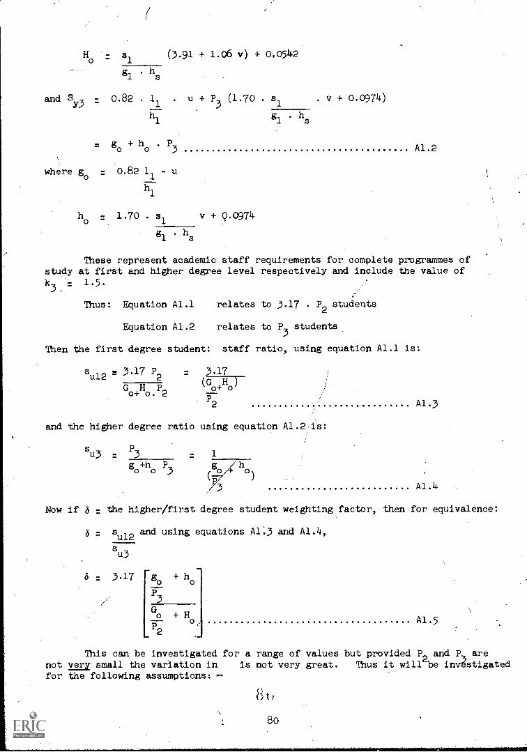
- s1

(3.91 + 1.06 v) + 0.0542

g1

. hs

and 3 0.82 . 1 . u + P (1.70 . sY3 1 3 1

h1

g1

. hs

= go + ho . P3

where go = 0.82 11 - u

19

LI.

. v + 0.0974)

ho

1.70 . s1

v + 0.0974

g1

. hs

A1.2

These represent academic staff requirements for complete programmes ofstudy at first and higher degree level respectively and include the value ofk3-

- 1.5.

Thus: Equation A1.1 relates to 3.17 . P2 students

Equation A1.2 relates to P3

students

Then the first degree student: staff ratio, using equation A1.1 is:

su12

- 3.17 P2

- 3.17(5ff-T-

G coH P2o

+ o. 2P2

and the higher degree ratio using equation A1.2fit:

su3

P3

go+h

oP3

A1.3

Now if a 7: the higher/first degree student weighting factor, then for equivalence:

= su12

and using equations A1.3 and A1.4,

su3

3.17 go + ho

P3

Go + H

o,

2

Al.

This can be investigated for a range of values but provided P2 and P33 arenot very small the variation in is not very great. Thus it will be investigatedfor the following assumptions: -

8t.

8o

For average annual intakes of.

P2 502

- P3 - 20

then 6 = 3.17 [0.05 go 4-

0.02 G Hoo A1.6

and when P2

and P3

are very large (i.e. go

and Go

are small compared with ho

and

PP32

H respectively) then:

61.7.. 3.17 h

o

H A1.7

Thus using equations A1.1, A1.2, A1.6, and A1.7 together with theparametric data from table 12 of section 2.2. the ft-flowing values of 6 are

obtained:

Table 20. Weighting of Fundamental/Advanced Level Students

Subject /

GlassiflationGo -

Ho

goho 5

61

Pure Science 2.53 0.376 0.615 0.285 2.34 2.40____

Technology 3.18 0.351 0.920 0.252 2.28 2.28

Med. Science 3.83 0.372 0.977 0.230 1.97 1,:96

Hum./Arts 2.49 0.220 0.696 0.187 2.49 2.69

Education - '2.12 0.214 0.598 0.176 2.55 2.60

Soc. Sc./Law 3.42 0.196 0.951 0.168 2.57 2.72

All 2.89 0.287 0.808 0.205 2.28 2.27

It will be observed that the values of S are reasonably consistent and give

values, between 2.0 and 2.7 with an overall of 2.28. These are in good agreement

with the order of values usually quoted for higher/first degree student weightingsand hence are some justification for the staff teaching load factor assumption

of k3 1.5._

Appendix A2

Analysis of Relationships between Departmental Academic Staff, Support

Area, and Supporting Staff.

A2.1. Relationship of total academic staff to supporting staff

From the data source of reference 1, for faculty and departmental level, the

following proportionality values were obtained for four broad subject groups.

8 i

81

Table 21. Ratio: Supporting Staff/Academic Staff Ds 2 d

DA

Group 1

Science

Group 2

Technology

Group 3

Arts/Social Sciences

Group 4

Medical Sciences

0.97 0.33 0.135 0.75

0.73 0.78 0.103 0.52

0.50 0.56 0.055 0.83

0.42 0.71 0.059 0.70

0.75 0.56 0.122 0.77

o.34 0.66 0.136 0.31

0.41 1.16 0.042 1.00

0.42 0.48 0.093 0.36

0.65 0.37 ' 0.250 0.48

1.19 0.79 0.290 0.42

1.28 1.48 0.046 0.45

0.52 0.68 0.166

1.06 0.0o

0.43 0.016

0.72 0.040

0.66

0.28

Average Average Average Average

o.68 0.69 0.106 0.60

A2.2. Relationship. of Departmental Support Area to Support Staff

Values of support area Al, are plotted against support staff NT for furbroad subject groupings in grapffs 2-5. These indicate good linearity especiallyat the lower end of the range, which is the most usual circumstance. Since,the values plotted represent over 70 items of data from about 12 differentcountries it will be apparent that geographical regional variation is not avery significant factor. Thus from the'slopes of the graphs:

Ab d

3105 for group 1

DS139 for group 2

77,for group 3

99 for group 4

8 o

82

(table 17)

A2.3. Relationship between Academic Staff, Laboratory Area and Supporting

Staff.

From equation (40) of section 3.2:

Ds = d1 .,Ab + 'd2 . DA(19)

also: Ab -b

d3 Ds d

D DA

Thus for (19) to be satisfied:

d, = 1 - d2

d3 d . d

3 A2.1

Hence if d2

can be determined then d1

can be calculated. A survey of thedata from reference 1 provided a quantity of information on supporting staff andacademic staff where the support area was zero (or very small). Since the d2

term will be small in equation (19) where support area is the dominating factor',this specific data was used in aggregated form to determine d2 (i.e. it beingassumed that geographical regional variation could be neglected).

Aggregated value of DS (Ab = 0) = 2.823

DA

Total number of observations = 40

Average value of D d2 2.823 0.07S

-2

4oDA

Thus equation A2.1 becomes:

d1 = 1 - 0.07d .d

4 A2.2

and using the group values of d3 and d4 above then:

d1 - 0.00855 for Group 1=

= 0.00647 for Group 2

= 0.00)04 for Group 3

= 0.00892 for Group 4

where: D - d A + 0.07 DS

d1 .Ab DA(19)

A2.4. Values of Support Area per Student

This data is derived from reference 1 in terms of support area per firstdegree/diploma student and the ratio of bigher degree/diploma support area tothis aF, (w).

83

zo

6

6/200/ 2 -reCHAfoLC.G

. 1!

I ....

-,:--

; .... ...t4.

!;:i

O

5"o fe7r) t 6-9tfPfill/2T/Ala -STAPP Ds

85

11 J

The values are presented in the following tables, categorized by the foursubject groupings used above.

Table 22. 'Values of Support Area per Student

Group 1Science

Group 2Technology

Group 3Arts/Social Science

Group 4Medical Sciences

co

m2

co

aF

m2

co

aF

m2

4.5 2.08 4.5 2.08 4.5 2.08 4.5 2.08

4.5 2.08 4.5 2.08 2.3 1.00 9.0 1.89

.6 2.40 4.5 2.08 6.o 5.84 15.0 1.24

.4 2.71 5.1 2.18 6.o 5.8 lo.o 2.50

.7 2.00 4.5 2.08 4.o 1.50 8.o 3.13

2.50 6.5 2.15 4.o 1.50 20.0 1.0R.!

.6 1.84 4.5 2.08 8.o 1.88 3.o 1.10

.2 2.40 8.0 2.5o 4.o 1.5o 6.o 2.5o

.4 2.34 8.3 1.87 5.o 3.00 5.o 4.00

5.9 2.24 4.o 4.25 7.o 3.86 5.o 3.2o

6.6 '2.o4 5.o 2.26

10.0 3.20

12.0 1.67

3.0 2.18

Averages Averages Averages Averages

2.26 6.1 2.18 5.1 2.8o 8.2 2.26

Averages for all groups: a, = 6.1 m2

avw = 2.36

aFX 2 aF = X 2 6.1

A2.3av

X20.79 for Group 1

1.00 for Group 2

0.84 for Group 3

11 1.34 for Group 4

88

A2.5. Method of Determining "Support" Area type Factor or

This method has been derived from section 3 analysis but using dataavailable from reference 1.. This is approximate only and the analysis of section3 would be better tested with new data in a specific study for the deterMinatiOn

of Gorr.

If TF

- Total average scheduled staff hoursdiplomas (lecture plus seminar)

TH

- Total average scheduled staff hours.diplomas (lecture plus seminar plus

given for first degrees/

given for higher degrees/research supervision).

Then using notation of section 2 and section 3.3.:

SH

k . TH . hsk . TH E (say) A2.4

(qT-SH)hs

TF3

T

Then: SH = E .,Sm

I-T7E-)

Using this in the equation of section 3.2. then:

(NT/ST

- 0.007)LI 0 x 2 =

[ii . a {2.364

Since all of the values in this exprlevel (except a which is for the university

A2.5

A2.6

ssion are given at departmentalas a. whole) then r can be determined.

A first evaluation of this is given i the followilig table for 10 broadsubject classifications and for individual s bject departments.

Table 23. Values of r b 0 Sub ect Fields.

SubjectField

r

Pure Sciences 0.91

Architecture 0.33Technology 1.04Medical Sciences 0.90-Agriculture 0.95Humanities 0.03Fine Arts I 0.06Education 0.17

Law 0.01

Social Sciences 0.15

These values are clearly of the right order but there are a number of

obviously wrong values. This is due to data inconsistencies and a further

analysis may yield better values.

89

For comparison the following values of r used by a particular U.K.university are given with appropriate similar oubject values quoted from the aboveanalysis.

Table 24. Comparison of ,'Derived Values of r .

Subject Area r (U.K.) r (Analysis)

Aeronautical Eng. 1.07

Chem. Eng. 1.00 1.18

Chemistry 0.67 1.08Civil Eng. 1.07 0.40Elect. Eng. 0.93 0.84Ergonomics 0.87Industrial Eng. 0.53Mathematics 0.20ech. Eng. 1.00 0.86

Physics o.80 0.79brary Studies 0.13 0.17

sign (Eng.) 0.47/

It.will be seen that in general the comparison is quite good and for thisreason it is suggested that in the absence of more accurate data the values fromthe analysis can be used as a guide.

CHAPTER 4. COMPARATIVE DATA ANALYSIS

1. Introduction

Page No.

2. A Brief 15-University Sample. Approximate Data Comparison

Part I. 2.1. Departmental Subject Data

2.1.1. General

2.1.2. Initial Survey by Subject Classification

2.1.3. Subject Classification with'GeographicalGrouping

2.1.4. An Approximate Cost Ranking of SubClassifications

Part II. Overall University Data

2.2. Population

2.2.1. Salary Ratings for all Staff' Categories

2.2.2. Some Student Ratios and Staff Distribution

2.2.3. Student Population and Weighting

2.3. Area

2.3.1. Land and Gros&Building Areas

2.3.2. Net Floor Unit'Areas

2.4. Finance

2.4.1. Recurrent Expenditure

2.4.2. Capital EXpenditure

Conversign Exchange Rates and ApproximateCost Ilidices

3. Further Data Observations on a'Larger International Survey

3.1. Overall University Data

3.2. Faculty Data

3.3. Evaluation of some Parameters of DepartmentalModel

Appendix A3. Aggregated Departmental Datafor all Sample Universities

91

1. Introduction

. The general purpose 'of the international comparisons of this chapter is topresent the trends derived from the 15-university sample and 80- university inter-national survey data. These provide a basis for the formulations of the overalluniversity data-based, and the more conceptualized departmental methodologievfChapters 2 and 3 respectively. At the same time some data interpretations noteof immediate application to the models, but pertinent to the general study ofuniversity management, are included.

The objectives of the data analysis may be set out as:.

(i) to provide a "first look" at compariadns between universities andgeographical regions at the overall university and departmehtal (subjectclassification) levels. This is especially true of section 2 below'.

(ii) to identify important parameters and variables with a major influence .

on resource requirements.

(iii) to provide background and data analysis for the simple more ,;conceptualmodel developed in Chapter 3.

Most of these objectives bear directly on the development of the overallsimplified university model (Chapter 2) and the more conceptualized departMentalmodel (Chapter 3). Where relevant reference is made to the specific sectionsof these models.

This chapter is divided into three major sections. The first, section 2,deals mainly with the derived values of parameters for the overall model ofChapter 2. This is based largely on the 15-university selected sample.Simultaneously certain comparisons and interpr4ations of data, not immediatelyapplicable to the overall model, but of general interest, are incorporated.

Section 3.2. concentrates on the 80-university survey. It does notrepeat the data constants set out in section 4 of Chapter 2, but provides furtherinformation, particularly related to departmental staffing, not available elsewhere.

In section 3.3., the evaluation of specific parameters of the departmental,

model of Chapter 3 is detailed.

2. A Brief 15-University Sample Approximate Data Comparison

As detailed in the introduction to this chapter, this sample analysis wascarried out with a view to identifying important parameters, to provide backgroundinformation, and to develop a simple methodology for data reduction for a morecomprehensive analysis.

The analysis is divided into two parts:

(i) data arising from the departmental level, /

(ii) data concerned with the university as a whole. These correspond"with sections 2 and 3 respectively of the model developed in Chapter 2.Where the data analysis provides insights for the model'or values forparameters, the appropriate section of the model is noted.

The small survey data is grouped into three geographical regions: NorthAmerica (N.A.), United Kingdom (U.K.) and Europe (EUR). Even with this verybroad classification, the samples are small, and the raw data contains a number ofobvious inconsistencies.

92 96

As far as possible the data has been revised, where available evidencepermits,'and various ratio parameters and percentages are frequently used to avoidscale effects and variable cost indices across countries. In addition, in order to

provide.an approximate basis for comparison,(especially on growth and cost) a simplecost index rating (Part II, section 2.4.3.) was developed from the overall universitydata and applied where appropriate. Where this has been employed the data is

referred to as "standardized".

It is emphasized that the information contained in this note should betreated with considerable caution and not used for qualitative studies. The

enlarged 80-university sUrvey,.some data from which is presented in Chapter 2,section 4, and in section 3 of-the present Chapter, is potentially useful forsuch studies. Nevertheless the information contained here can be of considerableusefulness, in providing initial approximate forecasts since data of the type andscope presented is not readily-available elsewhere.

Part I. 2.1. Departmental Subject Data (see section 2 of Chapter 2)

2.1.1. General

A considerable volUme of raw data, related to staff and student numbers,staff teaching hours and recurrent expenditures was gained from the survey. Inorder to present a reasonable overall picture it was decided to concentrate onnine selected items of data and analyse eight parameter ratios determined fromthis selected data. The data and parameters concerned are summarized in Table25 in the notation used throughout the overall model of Chapter 2, and the

following work. All departments were also classified into subject areas as

listed in Table 26.

2.1.2. Initial Survey by SUbject Classification

The values of A, B, C, eta. were calculated for each university and averaged

for each subject classification (i.e. aggregate averages at university level).This provided an opportunity of testing the reliability of the raw data atdepartmental level in relation to the overall university and to modify or omit

obvious errors. The overall data of Table 27 was thus compiled. At this stageregional variation was introduced and the raw data converted to a better degreeof consistency based on all the information available.

2.1.3. Subject Classification with Geographical Grouping

The full results of the above procedure are given in Appendix 1, for the

basic data (i), (ii) (iii) etc. bysubject classification and university, theactual values being the sum of all departments in a specific catagory and university.Into this data tables 28, 29 and 30 have been compiled. Table 28-is repeated in

table 1 of section 4, Chapter 2, substitution of.parameter values in the model.

Because of the small sample, some groupings cannot be regarded as representa-tive. The most reliable data is in Social Sciences, Education, Humanities,Technology and Pure Sciences for regional and general comparison. For individual

geographical groupings Law (in Europe), Fine Arts (in North AMerica) and MedicalSciences (in Europe) are the most significant although the samples are small andMedical is largely confined to dentistry, pharmacy etc., rather than medicine assuch.

The following observations are based on the information contained in tables

27, and 28 - 30.-

9 U

93

Table 25.

Selected Data for Single Departments in Specific Universities,

and Corresponding Parameters Analysed.

(1)

(ii)

(iii)

1(iv)

(v)

(vi)

(vii)

(viii)

(ix)

Total

Staff

(All Kinds)

Acad-

emit

Staff

Total

Teaching

Hours

First

Degree

Teaching

Hours

Total

Students

First

Degree

Students

Recurr-

ent

Expend.

Total

Standard

£ Equiv.

Total

Staff

Remun-

eration

Standard

£ Equiv.

Total

Academic

Staff

Remunera-

tion

Standard

£ Equiv.

DT

.DA

.TU

y FT

VT

VN

VA

ANALYSIS RATIO PARAMETERS

EF

GH

Acad.Staff

Total

First Deg,.

Students

First Deg.

Tot.Recurr.

Tot.Remun.

Acad.Rem.

Acad.Staff

(Teach.

Hours)

Total

f

(Teach.

Hours)

Tot.Staff

Acad.Staff

Total

(Students)

Tot. Staff

StandQ.d

£ Equi. ./

Staff

Tot.Recurr.

Standard

c.!. Equiv./

Staff

Acad.Staff

Standard

£ Equiv./

Staff

DA/DT

TT/DA

VT

1VA

Table 26. Subject Field Department Classification

Classification 1

PURE SCIENCES

Classification 5

AGRICULTURE

Classification 9

LAW

AstronomyBacteriology _

BiochemistryBiologyBotanyChemistryEntomology-GeologyGeophysicsMathematicsMeteorologyMineralogyPhysics.Zoology

AgriculturalbiologicalSciences

Classification 10

SOCIAL SCIENCES

Agriculturaleconomics

Agricultural.

physicalScienceS

.Animal husbandry.

Crop husbandry.

. Dairy farmingFisheriesFood TechnologyForestryHorticultureVeterinary

medicine

BankingCommerceDiplomacyEconomicsEthnologyGeographyHome EconomicsInternational

RelationsJournalismPolitical SciencePublicAdministration

Social WelfareSociologyStatistics

.

Classification 2

ARCHITECTURE

Classification 6 ,

UMANITIESHUMANITIESClassification 3

Archeology -----HistoryLanguagesLibrary ScienceiteratureLiterature

PhilosophyPsychologyTheology

Applied SciencesConstruction &.Civil EngineeringGeodesy

MiningSurveyingTechnologygy-Textile EngineeringElectrical EngineeringMechanical EngineeringChemical Engineering

Classification 7

FINE ARTS

Drawing'

MusicPaintingSculptureSpeech and_dramatic art .

Classification 4

MEDICAL SCIENCES

AnatomyDentistryMedicineMidwiferyNursingOptometryOsteopathyPharmacyPhysiotherapyPublic HealthSurgery

Classification 8.

EDUCATION

EducationPedagogyPhysical Education

ion

95

Pure Sciences: Supporting staffs are relatively large for all regions withN.A. somewhat leas so. In general they are abOut 40% of the total departmentalstaff. The teaching hours/staff are reasonably uniform at about 8.6.and some 75%are first degree students (With N.A. appreciably lower). The student/staff ratiois fairly variable (high in Europe and low in N,A.). The remuneration torecurrent expenditure ratio is reasonably uniform across the regions at about80%. : The cost per staff figures suggest that N.A. is somewhat high (probably dueto high post-graduate loading) and Europe somewhat low (probably due to somewhatlower salaries.of auxiliary staff).

Architecture: A poor sample. Support staff about half that for purescience (i.e. some 20%) but apart from this falls into a similar claSsificationto Technology and Pure Sciences.

Technology: Not a very large sample. Requires the most support staffof any classification*at about 45%. In other respects it is similar to purescience with slightly_higher_staff loadings and student/staff ratios.

Medical Sciences: A poor sample and mainly relative to supportingsubjects to medicine rather than medicine itself. General trends suggest highsupporting staffs (similar to Pure Sciences) low teaching loadings for academicstaff (2 - 4 hours /week) and relatively modest costs (but clearly does not includehospitals) although N.A. is markedly above U.K. and Europe -in this respect. Theproportion of post graduate work is high - about 45% to 50% - and this is particularlyso in Europe. T The high student/staff ratios suggest considerable teaching supportfrom outside sources.

ir

Agriculture: Only one sample from the N.A. region. The figures suggestthat it might be classified under Technology but the matter needs further investi-gation.

Humanities: Is fairly consistent across the three regions. .About 20%Support staff and some 10 hours /week academic staff teaching load with similarstudent/staff ratios. The higher degree proportion is reasonably large beingbetween 30% - 40%.: Recurrent expenditure other than salaries is small at about8% of the total recurrent expenditure.

Fine Arts: Again.a small sample. Generally requires a fairly largesupporting staff (about 35%) but with high academic teaching loads of some 13 hours/week. Higher degree population is similar to Pure Science and recurrent expenditureother than salaries is small'(about 14%), but larger than for Humanities.

Education: The support staff across regions is fairly uniform at about25% - 30%. Staff loading varies very widely as does student /staff ratio and theproportion of higher degree work. This latter is probably the key to the varia-tions (as costs also vary. considerably).

Law: Information here is predominantly European although the single N.A.example follows similar trends. Apart from higher support staff the results aresomewhat similar to those for Humanities. The higher student/staff ratiosprobably reflect a high degree of outside academic support plus appreciableservicing from other classifications. In general academic staff remuneration ishigh.

Social Sciences: Although not numerically the largest group this classifi-cation provided the best overall sample. There is a high.degree of uniformityacross regions with support staff at about 20% - 25% of total staff, academic staffloading at about 9 hours /week and some 25% higher degree proportion.

9

Table 27.

Selected Overall University Ratios Classified by Subject Area.

Subject

Classification

AAcad.

BTbtal '

C

1st Degree

DStudents

E1st Degree

FRecurrent

G

,Remun.

HRemun.

Tbtal

Staff

Teach.

Hours

Acad.

Staff

Tbtal

Teach

Hours

Acad.

Staff

Tbtal

Students

Tbtal

Staff

.Recurr.

Staff

Azad.

1. P. Sciences

.583

8.16

.683

12.80

.779

'

2613

.802

2450

2. Architect.

.792

11.86

.766

7.58

.808

2178

.931

2712

. Technology

.547

10.56

.543

9.22

759

2783

.800

2910

4. Med. Sciences

.544

4.39

.367

13.10

.616

2701

.825

2521

5. Agricult.

.625

0.57

.319

11.37

.721

3006

932

3726

6. Humanities

.813

/9.57

.686

8.38

.728

2666

913

2703

7. Fine Arts

.794

18.43

.830

3.91

.651

1

2907

899

3304

B. Education

.739

10.93

-377

12.60

377

2866

.788

2656

9. Law

.713

10.01

.681

23.38

.816

2870

.890

3171

10. Social

Sciences

.752

8.62

.654

19.18

.794

3046

.822

2874

Average

9.31

.591

12.15

.705

2764

860

2903

SELECTED DEPARTMENTAL RATIOS BY SUBJECT & GEOGRAPHICAL REGION

-'

TABLE 28'

,

1

CLASSI-

FICATION

GEOGt_-

GROUP REGION

A'

ACAD/

TOTAL

STAFF

.521

.771

.529

B

TEACH

HRS.

ACAD.

STAFF

9.34'

8.30

8.10

C'

1ST/TOTAL

TEACH HRS,

.609

.635

.661

D

STUD/

ACAD.

STAFF

7.83

4.75

11.92

EF

1ST/TOTAL

RECURRENT

STUDENTS

TOTISTAPP

*

.

......1

.811

3314.

.549

3573

.843

2051

G

TOT. ST,

REEUN

AST1771/

.808-

.831

.801-

H

ACAD.. RE NUN.

ACAD.STAFF. ---

.2819

3504

2214

-

1

Pure

Cc.

UK

NA

2BUR 8

Av

.607

0.58

.635

8.17

.734

2979

-,

..813

2846

2Archi-

tect.

UK

0NA

1

BUR 2

- .791

.802

0,53

12.20

.393

1.000

- 6.36

7.37

.424

3687

1.000

2604

.818

.821

- 3277

2358'

Av

.797

6.37

.697

6.87

.712

3146

.820

i

2818

3Tech.

UK

2)

NA

2

EUR 3

f.519

.549

.579

11.34

1:97

12.70

.619

.295

.889

10.69

7.48

10.55

.629

2484

.419

2790

.984

2831

.811

.909

.709

-----i

2904

2960

2500

Av

.549

8.67

.601

9.57

.744

2702

-

.810

2788

4Med.Sc

,

UK

NA

1)

EUR 5)

.500

,.780

.589

4.13

0.63

1.96

,.611

.700

.376

3.66

13.47

15.74

.734

2487

.942

3732

.208

1898

4778

.850

.824

2668

.

-

3781

1563.

Av

.620

2.24

.562

10.96

.628

2706

.817

2871

5Agric.

UK

0NA

EUR 0

:625

0.57

.319

11.37

.721

3006

.932

t-----7 .932

3726

3726

JAv

.625

0.57

.319

11.371

.721

3006

FTLLE

28

CONTINUL

CLASS.

GROUP

AB

.

CD

EF

'

'G

.

H

6'

UK

.833

11.00

.916

10.00

.938

2371

.958

2563

Hum.

NA

3)

r)

.837

10.08

.724

10.71

.354

3397

.912

3433

EUR 6)

.784

9.67

.682

11.09

.582-

2186

.879

2429

Av

.817

10.25

.774

10.60

.625

y

2651

.?16

2808

7UK

0-

Pine

rA

2.609

18.65

.828

5.64

.742

2740

.855

3583

Arts

EUR 1

.718

6.98

.696 -

15.21

.739

2551

.874

2607

Av

.664

12.82

.762

10.43

.741

2646

I

.865

2595

82

.696

11.19

0.000

5.81

.000

3043

.643

2500

:due.

NA

2.780

20.31

0.425

23.26

.736

3515

.830

3026

EUR 3

.738

8.24

.617

12.38

.643

2180

.827

1956

Av

.738

13.25

.347

13.82

.460

2913

.767

2494

9UIC.

0-

--

Law

NA

1.512

6.36

1.000

18.59

1.000

3326

.944

4545

EUR 6

.739

11.88

.516

20.93

.667

2633

.895

2771

Av

.626

9.12

.758

19.76

.834.

2980

.920

3658

10

UK

3.7

4010

.49

.737

9.12

.723

2595

.881

2725

Soc.

11.95

.754

3824

.829

2890

Sc.

EUR 8

.720

'

7.11

.659

16.90'

.784

2747

.780

2458

Av

'755

8.89

.669

12.66

.754

3055

,

.830

2691

OVERALL

AV

UK

.634

9.58

.582

7.85'

,673

'

2716

.813

2730

NA

.706

8.75

.593

11.59

.664

3359

.873

3473

EUR

.689

8.76

.677

13.57

.717

2409

.823

2362

1

1,7c-regated Av.

i.676

19.03

.617

11.004 .685

2828

.836

2855

Th=? fiTares in brackets by UK, NA, etc. is the sample number of classifications available.

SELECTED DEPARTMENTAL RATIOS ..AGGREGATED AVERAGES; BY SUBJECT.

TABLE 29

SUBJECT

CLASSIFICATION

A,

ACAD.

BTOT.TEACH.

HOURS

C1ST DEG.

TT 71

'_`:EACH.

,hoURS

DSTUDENTS

Ei

1ST DEG.

FRECURR,

GREMUN.

RECURR

HREEUN.

fOT.SAFF

AM.

,

-STAFIe

TcraT

0:'-t:DENTs

Mr

STAFF

STAFF

ACADEMIC

01-07:

1 P.Sdiences

.553

8.32

.648

10.26

.824

2414

.806

2493

2 Architect.

:798

7.58

.983

6.97

.792

3036

.820

2724

3 Technology

.556

8.00

.768

9.29

.765

2753

.811.

2758

4 Med.Sc.

.591

2.07

.437

14.19

.288

2105

.820

2234

5 Agriculture

.625

.57

.319

11.37

.721

3006

.932

3726

6 Humanities

.803

9.93

.715.

10.89

.536

2753

.897

2756

7 Pine Arts

.768

14.54

.740

3198,

.861

3239

.806

9.01-

8 Education

.768

17.94

'

.424

20.62

.716

3272

.819

'2832

9 Law

,

.716

11.48

'

.5315

20.76

.689

2704

.901

2901

10 Soc.Sc.

.747

8.20

.703

13.21

.764

3027

.822

2909

Av.

.693

/8.86

.634

12.66

..684

2827

.849

2857

AGGREGATED AV. *

.643

8.89

.671

11.67

.703

2658

.831

'

2694

-.--,

*Averaged by aggregating all departmental data for the

individual classifications

or4J4uTED DEFARTMENTAL DATA - OVERALL AVERAGES (Corresponding to

.,

table 5)

TABLE

30

.

UBJECT

(i).

(ii)

(iii)

(iv)

(v)

(vi).

(vii)

.(vij.i )

(ix).

LASSIPICATION

TOTAL

ACRD

Tf.:LT,

i-7:4T D:G.

TOTAL

i1;71;: LEG,TOTAL

TOT

TOTAL

STAFF

STAFF

'TEA:a..,

-

T_;!! CH

STUD=

S'OEDIT

IRECURREI:1

STAF1

ACAD.

2

.HOURS

HOURS

REMUN

STAFF

DT

Der

TT_.

T 11

,

.

F11

Vu

-

-

v,

REMUN.

1331

183

1521

986

1875

1545

713000

643000

45G000

256

45

339

.333

311

247

170000

139000

122000

3264

147

1175.

902.

1364

727000

590000

405000

- 1044

483

49

101

---

44

-693

200

174000

143000

109000

548

30.

.

17

i-5

341

-

246

144000

135000

112000

6164

132

1311

938

1437

771

453000

406000

364000

769

53

771

521

478

'

354,

.221000

190000

112000

854

.42.

.746

317

\357

613

177000

145000

118000

960

43

495

'

265

896

'

617

163000

147000

125000

10-

119

84

686

482

,1104

843

339000

278000

243000

.TOTALS

.

1248

808

7162

4893

9356

6480

3281000

816000

2126000

Recurrent expenditure other than remuneration is about 17% of the total.Student/staff ratio provides the greatest regional variation (being high in Europeand 16w in U.K.) and looking at these in conjunction with the academic loadings,suggests that the major difference may lie in the amount of individual work (private

study) the student is expected to do and-the importance attached to small group

teaching.

Overall Observations: These provide overall comparisons between regionsfor the aggregated classifications and in general show remarkably similar results.The values, with variational percentages irrbracke-ts, are given below:

[

Support Staff: 32% + 5% of total departmental staff.

3%

Academic Loading: 9 hours/week + 6%

- 3%

Higher Degree Work: 38% + 5% of total- 4%

- 28d[

Student/Staff Ratio: 11.0 + 23%

Tbtal Recurrent/Tbtal Staff: £2830 (equivalent standardized) + 19%- 15%

"Other" Recurrent/Tbtal Recurrent: 16% i

[

i. 4%

- 2%

[

Academic Salaries: £2860 (equivalent'standardized) + 21%- 17%

Thus the major departures are in student/staff ratios where Europe ishigh and U.K. low and in recurrent costs per staff and academic salaries both ofwhich mainly reflect large salary variations with N.A. high and Europe low.

Finally it should be observed here that data similar to that in tables 28 - -30and Appendix A3 could be used to investigate at the disaggregated.level some of thefactors considered in Part II for the overall university.

2.1.4. An Approximate Cost Ranking of Subject Classifications

AlthoUgh the "coat" of various subjects must be a matter for more detailedconceptual and data analyses based on the comprehensive questiOnnaire it is possibleto use the results in the previous sections to give an approximate guide as to the-cost

rankings of the various subject classificatiOns by regional groupings.

The method adopted here was to use merit ranking' numbers for each of theparameters A, B, C, etc., in order of costliness and to sum these to provideoverall rankings: Some considerable thought was given to the individualimportance of each parameter and guide table 31 was then constructed. Factors

are weighted equally for the ranking exercise.

Table 32 presents the results of.table 28 on a geographical region basisfor each aubject classification (and incidentally, follows comparisons withinregions). Summing the rankings for each parameter (together with those oftable 29) gives the following overall rankings:

0

102

METHOD OF SUBJECT CLASSIFICATION COST RANKING

TABLE 31

PARAM-

'?TER.

CONSTITUENTS

OF

PARR! TM

* COST

ORDER

,

RIT-A3E3

.

A' ACAD. STAFF

HIGH

Eeasure of supporting staff costs

,

High value -)low numbers

low'` .cost.

.

TOTAL3=7'

...

..

...

BTOTAL TEACH

HIGH

I:easure of acadtmic staff loading

High value -iless staff -*lower cost,

hOURS

ACAD.3TAFF

CFIRST DEG.

HIGH

Leasure. of Higher degree loading

High value }low higher degree load 7,:>lower cps-

TOTAL

(r.CEACHING

HOURS)

DSTUDENTS

ITAUTTEAFF

HIGH

Measure of academic staff numbers

High value -fewer staff -lower cost.

FIRST DEG.

HIM-

heasure of higher degree student numbers

'High value

fewer higher degree students ->lower cost.

°TOTAt

.

OTUDEITTS)

F _L!

TOT.RECURR

TOTAI 8TA3T

LOW

Low value -) lower cost

GTOT.REMN.

HIGH

Measure of "other' than remuneration relative costs

High value -;>"other" costs low ->lower costs.

TOT.MOVRR

H-----

TOT.REITUN

LOW

Low value "lower cost,

..

.t.

TOT.ACAD.

STAFF

(ACADEKIC)

/* Denotes whether high or low value of the parametercontributes to

least overall oost.

Ranking/in order of increasing costs:

T.K. N.A. EUR. ALL

° 6 ------.9.

3 8 -

10 6' 8\

6 7

1 10

4 . 4

.5

1=

2

2 6 Humanities

16 9 Law

2 Architecture,

9 1 Pure Science

1 7 Fine Arts

7 10 Social Sciences

4 8 Education

'110 4

3

Medical Sciences

3 Technology//

5 Agriculture i

The ntmbers represent subject classification and can be identified from the

right-hand column.

It/is emphasized that the above is a very rough guide but does elicit someinteresting factors. Of the principal subject classifications Humanities isrelatively least costly with Education nearte this but quite costly in the U.K.(probably associated with high post-graduate content). Pure Science is relativelycostly in U.K. and N.A. but less so in Europe, Technology is less costly thanPure Science in the U.K. (a surprising and probably erroneous result) but is aboutas costly As Pure Science in N.A. and is the highest'cQst in Europe. SocialSciences are of average cost generally but high in Europe.

Of the remaining significant clasiifications Law is relatively of low cost,. Fine Arts falls between the costs of .Humanities and Social Sciences and Medicine,although not very representative,,is generally costly.

Architecture and Agriculture areof !little Significance in these rankingsbecause of the very small. samples involved4

Part II. Overall University Data

2.2. Population

2.2.1. Salary Ratin for all Staff Categories (relevant to section3.2. of model of Chapter 2) .

No ebst index is incorporat in table 33. However the final column ineach.category is independent of s. There is an appreciable agreement in theaverage figures for the U.K. and rope although the latter includes two largishvariations (one is a specialized and somewhat costly institute and the other is anEastern European university with a low cost index and these tend to balance one*nether). The North American (N.A.) values vary appreciably (a small sampleanyway) but the averages are appreciably higher reflecting the higher cost index.Also apparent for N.A. is the narrower spread of salary range between all kinds ofnew-academic staff levels (this also applies to the East EUropean university).

1 1 u

104

TA

BL

E 3

2

Rat

ioparameters for subject classification

by geographical Groupings

REG-

I0/.1

CLASSI-

FICATIOK

(1)

(t)

1?ATIQ PARAtITI2M-3

,

..

Uf.

1.5

219.

34.6

097.

83*-

,811

.331

4' _

.808

.28

193

.519

11.3

4...

LIP

,10

.69

.329

2484

..811

2904

4..5

004.

13.6

113.

66.7

3424

87.

.778

2868

6.8

3311

.00.

.515

10.0

0.9

3823

71,

.958

..2

563

8.6

9611

.19

.000

5.81

-.0

0030

43-1

-1;6

4325

.00

10.7

40.

10.4

9.7

37.

-9.1

2.7

2325

95.8

8127

25

-.v'irk2

6101

111M

ISM

it:1

1111

1EM

IIT

A1

.771

:8.3

0.6

354.

75.5

4935

73.8

3135

042

.791

0.53

.393

6.36

.424

3687

.818

-32

773

.549

1-1.

97.2

957.

48.4

1927

90.9

0929

604

.780

0.63

.700

.-13

.47

.942

3732

.850

3781

5.6

250.

57.3

1-3

11.3

7.7

2130

06.9

32.

3726

6.8

35'

10.0

8.7

2410

.71

.354

3397

.912

3433

7..-

609

18.6

5.8

28,

5.64

.742

2740

.855

3583

8.7

80.

'20.

31.4

2523

.25

.736

-35

15.8

3030

26.

o ).5

12-.

6.36

,1.

000

18.5

91.

000

3326

.94

4x:'4545

10.8

04.

9.06

..610

11.9

5.7

5432

4.8

2928

90Av

.7b6

8.75

.593

117.

57-

....0

STM

.13u2

1.5

29.8

.10

.651

11.9

2.8

43-

2051

.801

2214

2.8

02-1

2.20

-1.

000

7.37

1.00

026

04.8

2123

58.3

.579

12.7

0.8

8910

.55

.984

2331

.709

2500

-.:4

.589

-1.9

6.3

76.

15.7

4.2

0818

98.8

2419

636

.784

9.67

.682

11.0

9..5

8221

86.8

7924

297

.718

6.98

;695

15.2

1.7

3925

51.8

7426

078

u.7

38.

8.2.

4-.6

1712

.33

.643

2180

.827

1956

9.7

3.9

11.8

8.5

1620

.93

.667

2633

.895

2771

10.7

207.

11.6

5916

:90

.784

2747

.780

2458

Av

.>

77f3

.57

..I

.3

2 o

The following presents a brief summary of the main features of the table bycategory although it should be observed that the definition of staff levela varyconsiderably between, and even within, countries and a study in depth of this wouldproduce more, consistent data.'

--Academic Staff: Close agreement between U.K. and D.rope with professorial

salaries some 70% greater than overall academic average.,. The N.A. region pro-fessorial Salaries are some 100% greater (and contrasts sharply with the narrowersalary spread for other categories).

Administrative Staff: The average administrative salanies are about halfthe average academic salaries. in U.K. and EUrope although there is a greater spreadin level in the U.K. The administrative salaries in N.A. are cunparable with theacademic salaries although slightly lower (about 5% - 10%).

I

Library Staff: Average library staff salaries are about the same as averageadministrative salaries in the U.K. and Europe but some 20% lower in N.A. Howeverthe library situation depends on the importance placed on library provision,consequent facilities, responsibilities and size, and these need to be studied indetail.

Technical and Other,Staff: This shows the greatest variation betweenregions but is reasonably consistent within them. It is clearly a function of thetype of university (technological, general, specialized, etc.) and must normallybe viewed in relation to this function (this is apparent from the departmentalanalysia in Part I). There is also a need to distinguish between technical staffandothers since their respective functions are quite, different especially on thescience; technology and medical sides (where specialized support staff tend to be.a high proportion of total staff). The results shown, however; suggest thataverage salaries for technical and other staff in N.A. and Europe are about thedame as those fOr the average library staff with the U.K. some 13% loWer than this.In all cases the comparative top salary level is lower than for the other staffcategories and there'is less overall spread.

Total Employees:, The average salary quoted is clearly some reflection ofthe cost index of the various countries and, in particular, of the specificinstitutions (the latter on the theory that 'costliness' is often reflectedthrough salary levels). The ratings in the three regions vary fairly markedly -the average total employee salaries being about 60%, 100% and 80%of the averageacademic staff salaries in the. U.K., N.A. and Europe respectively. This appearsto stem largely from the relatively high proportion of Technical and other staff inthe U.K., of administrative staff in N.A. and of academic staff in EUrope (seedistribution of staff).

2.2.2. Some Staff' Ratios and Staff Distribution (relevant forsectibn 3.1. of model, Chapter 2).

From table 34, the following observations are pertinent.;

Staff ratios: These refer to administrative and librar only (academic isdealt with-under student /staff ratio and "Technical and Other " combined has moresignificance at departmental level). The library student/staff ratio is somemeasure of the service provided since student population is e most significantspecific group involved. The values vary widely between an within regionsreflecting the varying degrees of importance with which libtary facilities areregarded. High values imply_ nadeqUate facilities and here EUrope comes offworst (although probably exaggerated by very high values) with a ratio ofabout 150. The U.K. is about half this and N.A. just over one third. However

11.106

SALARY RATINGS FOR ALL STAFF CATEGORIES

TABLE

33r

REG-

ION

UNIV

U.K.

EUR.

AV 4 5 6

Av 7 8 910

11

12

1314

15

ME

Iv of «v

AC

*f4I

N A'

1.00

1.03

1.1

irrIC

1.05

2.34

1.11

1.23-

1.12

1.18

1.06

1.06

1.09

1.42

0.74

0.5

1.03

1.14

1.10

.717-

1.67

1.67.

1.76

1.70

1.

1.6

1.77

3.17

2.94

3.06

1.88

2.32

1.49

1.47

2.18

2.59

1.50

0.6

,1.77

1.97

2.20

1.68

-.

1.36

2.65

2.01

1.68

1.97

1.41

1.39

2.06

1.82

2.03

1. 0

1.70

1.74

ADMNISTRATION

LIBRARY

TECHNIC .A

OTHERS:

rD

"AX

*1 L

crL)

triz

0)

.51

D. 2

1.35

1.01

1418

.

58

0.58

0.58

0.44

0.50

0..44

0. 4

0.49

0.62

1.80

0.73

2.11

1.85

1.98'

2.35

2.09

2.22

0.87

1.52

1.52-

1.91

2.39

2.05

0.85

1.59

1.77

1.93

0.36

0. 2

0.34

0.40

0.62

0.51

0.43

0.47

0.52

C.40

6.39

0.28

O. 0

4.15

.5

3.86

1.74

2.05

1.90

1.49

2.63

2.59

4.48

4.81

4.61

2. 0

0.43

0.49

0.5

0.50

0.75

0.99

0:87

0.40

3.30

0.41

3.15

0.76

0.67

0.61

0.53

0.51

0.24

O. 0.52

0.57

1.48

1.52

0. 1.33

1.31

3.24

2.28

1.16

1.42

1.19

1.62

2.22

0.33

0.58

1.22

0.22

0.24

O. 0

0.25c'

0.50

0.51

1.43

0:51,

0.64

0.39

0.43

0.36

0.38

0.17

0.24

0.37

0.37

3.48

3.07

1.

2.77

1.76

3.29

2.53

1.52

2.11

1.95

3.03

4.33

1.39

1.

5

0.37

0.37

0. 8

0.37

0.62

1.18

0.90

0.68

0.54

0.59

0.38

0.77

0.53

0.2

0.77

0.64

O. 0,

0.77

1.33

1.59

1.46

2.30

0.53

Our

1435

0.67

0.82

1.26

1.97

1.04

0.40

1.07

0.18

0.26

0 1

0.21

0.41

0.78

0.60

2.05

1.76

2. 6

TOTAL E!.',771,:.;YEES

T:QUIv

rT

I

-

2.06

2.16

1.35

1.76

0.32

2.45

0.56

1.06

0.34

2.01

1780

1740

1j.

6417

60G

.65

3620

1.34'

2920

3270

1C

'1

2490

2200

2500

2010

3130

2370

1110

,f12

0.31

0.7.÷

3./11

'2.34

_J--

225u

0.42 3.02

0.63

1.61

0.38

2.53 0.60

1.10

0.38

1.94

234'0

233

A. rating of 1.00 relates to t2700 p.a. equivalent.

Rates of exchange used are 1968/69

values given in section 2.4,3.

a glance at the column does suggest that a ratio of about 75 is a reasonablecurrently acceptable level. The administrative staff/academic staff ratio issome measure of the administrative baCk-up support to academic staff and again isqUits variable. The figures-indicate that this back-up is least in Europe (about25%) is very high in N.A. (about 170%) with U.K. falling in between (about 6$).This follows the same pattern as for salaries except that the differences are more\marked on a personnel number basis.

Table 34. Ratios of Staff Numbers, by. Type of Staff

Region Univ.

Staff RatiosDistribution ofStaff % Numbers

Tot. Stud. Admin.Acad.

(nITT)

Admin.

(nITA)

Lib.

(mTL )

Tech.endOther

(mom)

Lib.Staff

(me)

Acad.Staff

(m D)

U.K. ,.1 44.4 . 0.28 43 14 8 352 86.0 0.55 39 I 21 4 36

3 83.5 0,95 30 28 4 38

Av. 71.3 0.59 37 21 5 37

N.A. 4 29.8: - - -

5 87.3 2.47 20 50 3/

27

6 41.3 1.00 31 31 2 36

Av. 52.8 1.74 25 40 3 32

EUR 7 343.6 0.17 68 12 4 16

8 109.2. 0.21 50 10 7 339- .:68.9 0.35 50 18 5 27

10 61.2 0.31 50 16 .6 28

11 83.8' 0.38 49 19 4 28

12 l' 98.84 0.49 53, ' 26 '15 6

13 318.7 0.12 33 . 4 1 6214 10:9 0.23 69 16 3 1215 .133.7 0.23 52 12 5 31

Av. 151.0 0.28 52 15 6 27,,.

Overall Av. 115.4. 0.55 46 20 5 29

Av. of Avs. 91.7 0.87 38 25 5 32

Distribution of Staff:- The last four columns of table 34 present this aspercentages of the total for academid; administrative, library and "techniciansand other" staffs. Library staff is about 5% generally and the lower figure forN.A. could well represent an economy of scale since the absolute staff numbers arerelatively high. The:Technician and Other Staff shows a relatively modestvariation in terms of,percentage of the total staff (37% in the U.K. to 27% inEurope) but expressed as a proportion of academic staff it represents about 1 peracademic staff member, 1.25 per academic. and 0.5 per academic for U.K., N.A. and

EUrope respectively. The greatest variations however occur between academic

114 io,s

and; administrative staff percentages. Combined they represent 60% - 65% of the

total staff for all regions but individually they are 37%, 25% and 52% for academic

staff and 21%, 40% and 15% for administrative staff respectively for U.K. N.A. and

Europe. The major difference in staff distributions between regions seems to be

the degree of administrative support.

2.2.3. Student Population and Weighting

Table 35 is deduced from the overall raw data which in some instances departs

considerably from the incrementally summed departmental data and must therefore beviewed with smile suspicidn from the outset. However it can provide.an approximatepicture relevant to the basis of the general model, outlined in'section 3, of

Chapter 2.-'

Student/Staff d Student Level Ratios: The student/staff ratios (s u) vary

considerably across d within regions with the average values being about 9, 8.5

and 11 respectively fo the U.K., N.A. and Europe. It is perhaps unfortunate that

this ratio often aJsum s exaggerated importance as a measure of university,

efficiency whereas ysis shows it to be a complex function of many university

data variables. Howe er as .a refinement, it is often associated with the level

of higher degree to first degree work and for this reason the second column in .

table 11 presents this ratio. Before relating this to student/stafk\ratio it is

worth noting that the overall figures give approximate higher/first degree ratios

of about 22%, 55% and 48% respectively for the UK., N.A. and Europe. The level

of "effective post-graduate" work in Europe and N.A. is about twice that in the

U.K. If it is assumed that higher, degree work is more demanding (and al more

costly) on staff time then a high level of higher degree work will imply a low

student/staff ratio and vice-versa. In table 35 it will be seen that although in

a number of cases this implication is substantiated there are also sufficient cases

to the contrary to suggest the need for a much more elaborate analysid. Additionally

in the case of Europe tbere is considerable doubt as to what constitutes firdt andhigher degree levels, a ("first degree") diploma often taking several years more to

complete in Europe than in the U.K. or N.A. All of this suggests that thede two

ratios taken on their own are not a very reliable guide to overall university,

comparison. Nevertheless it was considered worthwile to extend the analysis hereto determine whether "weighted" student/staff ratios showed a better correlation

and to gain some idea of the approximate relative weighting factors.

Student Weighting: A. simple. analysis yields the following relationship:

-aa2+Xw (1)

where al - First degree student/staff ratio based on total staff,

a2

Higher degree student/staff ratio based on total staff

a RelatiVe weighting of 1 higher de ree.to 1 first degree student.

w7. Weighted student/staff ratio based on total staff.

Values of a1

and ao are given in table 35. Clearly ifwand a are

constant within regions then plots of al against a2 will be linear and yield values

for these constants. This was done and provided graphs containing considerablescatter although the trends suggested the negative slope of equation (1). Mean

lined.gaVe the very rough values for a and X presented on table 11 for the

various regions. Obviously the values for U.K. and 11:k can have no statistical

significanbe because of the small number of samples. The weighting factors vary

from about 1.6 to 4.3 for the regions but the overall value of approximately 2 is

109

.-

,.

THE DISTRIBUTION OF STUDENTS TO ACADEMIC STAFF

TABLE 35.

OVERALL

:HIGHER

FIRST DEG.

HIGH DEG.

WEIGHTED

REGION

UNIV

STUDENT/

DEGREE

STUD/STAFF

STUD/STAFF

WEIGHTING

STUD/SWF

STAFF-

to

RATIO

,RATIO

,-

FACTOR

'

RATIO.Asuy

RATIil

.-

FIRST DE.

al(=.;U)

64.2(= iG)

.pc= AV VALUE

(a =

T_)

RATIO (pa)

TFOR REGION.

U.K.

1f3.52

,0.170

-

7.27

1.25

(3.34)

11.4

28.23-

0.213

6.62

.1.40

(3.34)

11.3

.

'

310.30

0.267

8.13

2.19

(3.34)

15.4.

Av

9,02

0..217

7.34

1.61

3.34

12.7

4(9.77)

0.480

'(6.60)

(3.17)

(4.32)

'

20.3

512.70

'

.0.216

10.50

2.27

(4.32)

'

. 20.3'

62.98.

0.965

1.52

'

1.46

(4.32)

7.8

Av

8.46'

0.554

6-.21

-

2.30

4.32

16.2

7 819.20

15.80

,

-

0004

0.819

19.17

8.54

0.08

6.99

p.63)

1.63)

-

19.3

19.9

BUR.

'

97.23

'

'0.364

5.28

1.92

.1.63)

8.4'

10

7.43

'

-0.040

7.15

0.30

1.63)

7.6

11.;

6.86

0.651

4.14

2.70

1.63)

8.5

12

27.10

2.020

9.00

18.16

1.63)

38.6

1.3

'

8.45

0.115

7.57

'

0.88

1.63)

9.0

5.93

0.942

2.23

2.11

1.63)

5.7

15

12.40

(0.000)

(12.40)

(0.00)

(1.63)

12.4

Av

11.16

0.441

8.38

3.68

'

1.63

14.4

Overall Av.

10.80

0.484

-

7.76

2.91

'

1.96

13.5

.

Figures in brackets are estimated values.

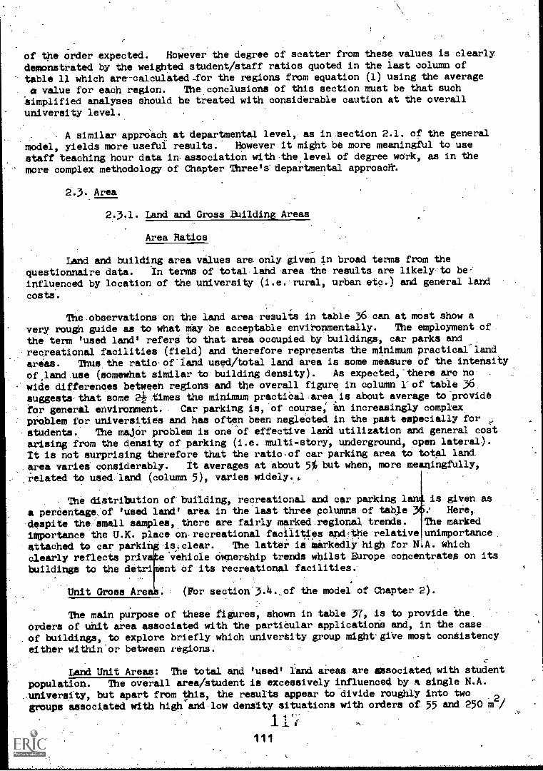
of the order expected. However the degree of scatter from these values is clearlydemonstrated by the weighted student/staff ratios quoted in the last column oftable 11 which arecalculated-for the regions from equation (1) using the average

. a value for each region. The conclusions of this section must be that suchSimplified analyses should be treated with considerable caution at the overall

university level.

.A similar apprdich at departmental level, as in section 2.1. of the general

model, yields more useful results. However it might be more meaningful to usestaff teaching hour data inassociation with the level of degree work, as in themore complex methodology of Chapter Three's-departmental approacW.

2.3. Area

2.3.1. Land and Gross Building Areas

Area Ratios

Land and building area values are. only given in broad terms from the

questionnaire data. In terms of total.land.area the results are likelsvto beinfluenced by location of the university (i.e. rural, urban etc.) and general land

costs.

The observations on the land area results in table 36 can at most show avery rough guide as to what'may be acceptable environmentally. The employment of

the term 'used land' refers to that area Occupied by buildings, car parks andrecreational facilities (field) and therefore represents the minimum practical land

areas. Thus the ratioof'land used/total land area is some measure of the intensity

of land use (somewhat similar to building density). As expected,' there are no

wide differences between regions and the overall figure in column l of table 36.

suggest,futhat some 2' times the minimum practiCal.areais about average to provide

for general environment. Car parking is,'of course, an increasingly complex,problem for universities and has often been neglebted in the past especially for

students. The maj.Or problem is one'ofeffective land utilization and general costarising from the density of parking (i.e. multistory, underground, open lateral).

It is not surprising therefore that the ratiOof car parking area to total lanl

area varies considerably. It averages at about 5% but when, more meaningfully,.related to used land (column 5), varies widely.g.

The diltribution of building, recreational and car parking 1 is given as

a perCentageof 'used land' area in the last three polumns of table Here,

despite the small samples, there are fairly marked. regional trends. The marked

importance the U.K. place on. recreational facilities.anth.the relative unimportance.attached to car parki isclear. The latter is airkedlk-high for N A. Whichclearly reflects priv evehicle ownership trends whilst Europe concentrates on itsbuildings to the detri brit of its recreational facilities.

Unit Gross Are (For section.3.4.,of the model of Chapter 2).

The main purpose of these figures, shown in table 37, is to provide the

orders of unit area associated with the particular applications and, in the caseof buildings, to explore briefly which university group mightgi've most condistencyeither within-or between regions.

Land Unit Areas: The total and 'used' land areas are associated with student

populatiOn. The overall area/student is excessively influenced by a single N.A...university, but apart from this, the results appear to divide roughly into twogroups associated with high and low density situations with orders of 55 and 250 m2/

1 1

111

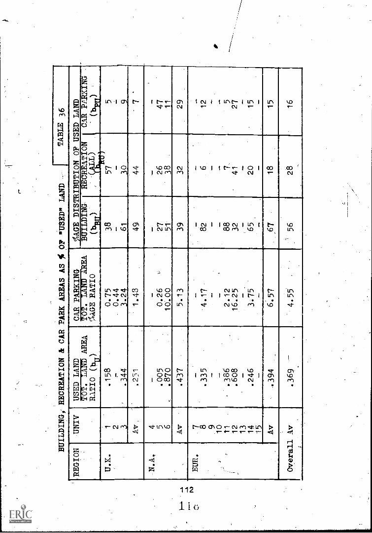
BUILDING RECREATION & CAR PARK AREAS AS % OF "USED" LAND

iTABLE 36

REGION

UNIV

-

USED LAND

CAR PARKING

TOT. LAND AREA

(10AGE RATIO

_AGE DISTRIBUTION OF USED LAND

TOT. LAND AREA

RATIO

(bu)

BUILDING.

(btu)

RECREATION

CALL)

CAR PPRK.ING

'

(bin!)

U.K.

1 2 3-

.158

,.

.344

0.75

_0.44

3.24

38

61

57

30

5 9

Ay,

.251

-

1.43

49

44

N.A.

4 5 6.005

.870

0.26

10.00

27

-

51

26

'

38

47

11

Av

.437

5.13

39

32

29

E,..

,7 8 9.

10

ti

12

1314

15

.335

.386

.608

.246

'4.17

-,

2.12

16.25

3:15

82

88

32 65,

--

6.- 7..

'

41 20

12 5

27

15

Av

..394

6.57

67

18

15

Overall Av

.369 -

4.55

*

56

28

16

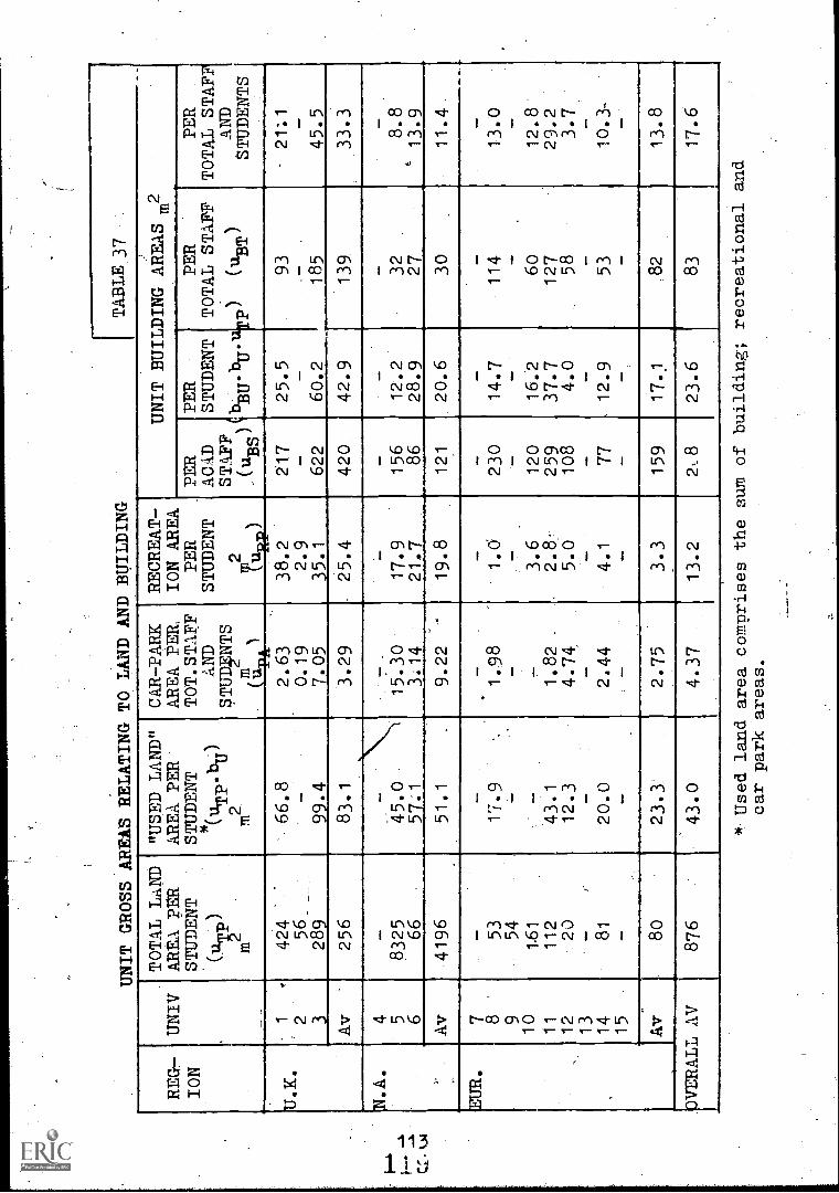
REGr-

ION

UNIV

UNIT GROSS AREAS RELATING TO LAND AND

TOTAL LAND

AREA PER

STUDENT

(1p)

"USED LAND"

AREA PER

STUDENT

*(uTp.bu)

m2

2 3

Av

424

56

289

66.8

99.4

CAR-PARK

AREA PER,

TOT. STAFF

AND

STUDFITS

(111114r1

2.63

0.19

7.05

256

83.1

3.29

BUILDING

RECREAT-

ION AREA

PER

STUDENT

m2

fuRp)

38.2

2.9

15.1

25.4

4 5I

8325

666

45.0

57.1

Av

4196

51.1

15.30

3i14

9.22

17.9

21.7

19.8

7 8 910

11

12

1314

15

5354

1.61

11220

81

17.9

43.1

12.3

20.0

1.98

1.82

.

4.74.

2.44

3.6

2.8:

5.0

4.1

Av

80

23.3

2.75

3.3

.aVERALL AV

I876

43.0

4.37

13.2

ITABLE 37

UNIT BUILDINGAREAS

m2

PER

ACRD

STAFF

(uBS

)

PER

STUDENT

, uBU'bU'uTP)

PER

TOTAL STAFF

(uBT)

PER

TOTAL STAFF

AND

STUDENTS

217

25.5

93

21:1

622

60.2

185

45.5

420

42.9

139.

33.3

156

12.2

32

8.8

86

28.9

27

13.9

121

20.6

30

11.4

230

14.7

114

13.0

120

16.2

60

12.8

259

37.7

127

29.2

108

4.0

58

3.7

77

12.9

53

10.3-

159

17.1

82

13.8

2 8

23.6

83

17.6

* Used land area comprises the sum of building;

recreational and

car park areas.

studentrespootiVely. The 'used' land uni areas are relatively more consistentand augsast an overall fisure of about 40 m /student (a little less than the N.A.figure) with the U.K: being about twice this and Europe about half. Car parkunit arras are asisociated with the overall university po ulation (staff andstudents) and again show wide variation with the same re onal emphasis referred toabove.

Table 38. Building Floor Area Ratios.

Region Univ.

Tbt., Build.

Floor AreaTbt. Build.Floor AreaPer Univ.Member

A i-P

T/NT T

m2/pers.

Tbt. Build.Floor AreaPer Tbt.Staff

AT/NT

m2/pers.

"Other" FloorArea Per Tbt.StSff Member

A m Up0T

m2/pers.

Tbt. Build.Land Area

dB = AT

BB

U.K. 1 0.842 16.84 78.15 47.16

2 13.09 54.85 22.74

3 0.252 11.48 46.77 25.71

Av. .547 13.80 59.92 31.87 .

;47. 4 - -- - -

5 1.785 15.77 56.50 42.48

6 2.522 3.85 66.85 43.69

Av. 2.154 23\36 61.68 43.09

RUB. 7 -

8 1.500 19.59 171.11 113.47

9

10 1.550 19.76 93.10 46.18

. 11 0.483 14.10 61.41 -

12 1.821 6.76 104.69 27.17

13 - 7/18 27.02 2.58

..14 2.976 3 .72 117.13 59.09

15 /

Av. 1.666 4 .m 95.74 49.7o

Overall Av. 1.526 16.93. 79.78 43.03

The overall value is about 4.4 m2 /member with N.A. over twice this figure.

However the more important consideration is the degree of availability of car

parking spaces. A measure of this can be determined from assumed values of'effective' area per car parking plage - this will usually vary from about 12 m /place in the U.K. and Europe to 15 m /place in N.A. and using these valuem implyabout 1 place for 4 university members in the U.K. and Europe and 1 plage for

(leas than) 2 members in N.A. Recreation unit Fees are about 20-25 m /student in

the U.K. and N.A. whereas they are Only some 3.1m /student in Europe which is

almost Oertainly inadequate. Moat of this refers to field area and there ismuch that can be done with the use of intensive "dri-play" areas and the like.

Building Unit Are-a: The overall area of abou 24 m2/student compares quite

favourably with the known average value of about 20 m /student for all universities

in the U.K. However a mean deviation calculation suggests that for parametricvariation purposes the best university group basis is either total or academicstaff which perhaps more accurately describes the full functions of the buildings.

2.3.2. Net Floor Unit Areas (see related to section 3.3., Chapter 2).

The raw data for table 39 was sparse and any deductions must be extremely

tentative. In general laboratory area per student shows little regional variation(with the exception of one N.A. university which is specialized gnd highly researchoriented) and fairly uniform values with an average of about 5 m /student.

Obviously the individual values will depend on the amount of science and technology

work undertaken and a further analysis at faculty level should elicit more reliable

information. .All teaching room space per student again shows comparatively

reasonable uniformity with Europe having ratheg more space than N.A. and U.K. (in

that order). The average value is nearly! m /student. Library area per

student is similar teaching room space per student for the U.K. and N.A. (and

is about 1.5 - 2.0 M/student) but is substantially leas for Europe (about half).kcadamic staff office space is fairly uniform across regions and is some 20 m /academic staff on average. Administrative staff office space is rather less than

academic staff space in U.K. and N.A. but appreciably more in EUrope. Obviously

this latter depends on the definition,of office space (e.g. whether it includes

machinery). The whole problem of office accomodation would benefit from adeeper analysis at faculty level since although it has relatively small effects

on overall university costs it is a vital matter concerning staff morale.

Building Density: _The values of building density are quoted in column 1

table 38% Since floor areas are net and land areas are gross it is possible to

obtain a value of dg lea's than unity (which would otherwise denote all ground-level

buildings only). There is no pariticular reason why there should be regionaldifferences and the samples are too small to provide these anyway. However the

total sample'appears to fall into three separate density groupings so that for an

approximation it can be deduced that:

dB _- 0.526 for a low average building density

dB

1.664 for a medium average building' ensity

dB 2.749 for a high average building density

and these values can be used to indicate the order of building density for any

corresponding values orbuilding floor area(AB) and land area (BB).

These values are those utilized in equation (41) of section 3.4. of the

simplified overall model.

12i

115

NET FLOOR UNIT AREAS

.

'

TABLE 39

REG

ION

UNIV.

LABORATORY AREA

PER

2STUDENTmoln

ALL TEACHING

ROOrS PER

STUDEIV)

LIBRARY AREA

PER

.

STUIJn

2-

ACAD. OFFICE

AREA PER

2

ADMIN.OFFICE

A.ARE PER

ADTTIN.STAFFm2

°In/

13.K.

1'

2.8

1.4

-

2.6

'24.0

42.8

26.2

1.7

0.6

14.2

5.8

32.8

1.0

1.4

17.0

16.0

Av

3.9

1:4

1.5

18.4

'

16.7

N. A

.4

.._

50.8

2.1

1.4

20.0

4.9

612.6.

'

1.9

2.0

16.1

16.1

Av

6.7

2.0

1.7

18.1

10.1

EUR.

7,-

78

5.1

0.8

0.8

9.3

75.2

99.9

10

11

4.9

.2.5

.

0.9

30.1

8.1

12

-'

2.6

1.6

50.4

36.7

13

3.7

2.9

0.3

12.8

53.6

14'

2.9

5.9

-

0.6

7.7

23.8

15

.

Av.

4.2

2.9

0.8

22.1

34.6

Overall Av.

4.6

2.3

1.2

20.2

26.6

2.4. Finance

2.4.1. Recurrent Expenditure (Related to section 3.2. of the overall

model).

Information on recurrent expenditure was relatively sparse especially in

the distribution of recurrent expenditure excluding remuneration.

The ratio of total staff remuneration to total recurrent expenditure isremarkably consistent both within and across regions and is of the order of60%65%. Since the difference betWeen the two quantities represents the recurrentexpenditure on non-salary items it is then evident that the expenditure excluding

salaries is about one-third of the total annual recurrent expenditure (i.e. about

half:_the-tctal salary bin).

Within the category, recurrent expenditUre excluding remuneration, theresults are very poor. .

On the administration and "other" percentages it would be unwise to draweven tentative conclusions other than between them they account for about 95% of

the total. The library percentage is fairly consistent at 5% overall with theN.A. values showing a possible economy in scale.

2.4.2. Capital Expenditure (Relevant to section 3.5. of the model

in Chapter 2) .

Table 41 sets out th annual average capital expenditures of the 15-

universities, classified b purpose of expenditure. A

Distribution of Total Averaged Annual Capital Expenditure: Capital

expenditure does not necessarily have any determinable relationship to recurrent

expenditure. Furthermore capital expenditure can vary enormously from year to

year according to grower::, economic climate, research, etc. Thus any analysis in

depth Should be time-dependent. It also follows that to explore the effects ofcapital on recurrent cost then time dependent data on recurrent costs is alsoneeded,-but this is not available from the survey.

Building capital expenditure for all regions, is quite high, indicating afairly high university growth rate during the period 1965,-69.. The average pro-

portion for building of total capital expenditure is nearly 70%. Thus remaining

capital for other purposes is about 30% overall but this almost certainly includes

somecapital resulting from the building programme.- Thus a major problem arises

in distinguishing capital expenditure for and arising from, buildings and necessary

or "true" capital expenditure associated with the university in its steady state.This problem is clearly demonstrated in the figures for adMinistration and library

'in table 42' hich in the case of/the former is almost certainly also influenced by

the inclusio of maintenance, minor extensions and alterations, etc. It is

therefore n possible to draw even rough meaningful conclusions from theAdministrat on and Library capital data although it appears that the "true" capital

costs are in the"region of 4% or -less of the total capital expenditure.

Relationship of Building Capital to. University Groth: The following simple

analysis is the basis of the growth factor utilized in section 3.5. of the simple

model of Chapter 2.

Growth is usually presented as an annual percentage rate based on student

number increase hence:.

12 t)

117

RECURRENT EXPENDITURE RATIOS AND DISTRIBUTION

TABLE 40

.

REG-

ION

UNIV.

TOT.'STAFF

REMUNERATION

TO TOTAL RECURR-

ENT-EXPENDIT.

RATIO (rT)

-

.58

.62

TOT. RECURRENT

(EXCLUD.REMUNERATION)

PER TOTAL STAFF

MEMBER EQUIV. £ *

.

(rinT

)

1645

1272

1058

%AGE RECURRENT EXPENDITURE

(EXCLUDING REMUNERATION).

-ADmIN.

(POD)

5.1'

6.

LIBRARY

(POL)

8.9

(4.1)

7.1

OTHER

(P00)

86.0

'86.6-

U.K.

1 2 3

Av

.

.60

1325

, 5.7

.,

8.0

4

86.3

N.A.

4 5 6

.53

.70

.61

-

1571

2348

1960

-

15.7

12.7

14.2

(1.8)

11.3

1.3

6.3

73.0

86.0

_795

Av

.61

EUR.

7 8 910

11

12'

13

14

15

- -.

.64

.59

.55

.

I-4T

-.

.46

.90

-

1250

1754

1613

-891

-

2518

128

3.2

17.8

- .. - -

(20.2)

__

- -

1.6

5.5

(2:5)

- - _

-.

-

95.2.

76.7

- - -

Ay

.65

'

1359

10.5

'3.6

85.9

Overall Av

.63

1457

11.5

4.9

83.6

(APPROX)

* Converted using rates of'-exchange for 1968/69 values given in Section 2.4.2.

AVERAGE ANNUAL UNIVERSITY CAPITAL EXPENDITURES

ITABLE 41

UNIV.

CURRENCY

TOTAL UNIVERSITY AVERAGE PER

YEAR (x 10

-3)

OF TOT. UNIVERSITY

AV/YEAR (x 10

-3)

.--------

TOTAL

BUITAINGS

OTHER

'AMIN.

LIBRARY

rg

:g

C1

I,

956

784

172

45

109

-

2£

637

405

232

66

':10

3R.

1675

971

704

11

.1.42

4"' Can.

6890_

6740

15a

14

1800

5t U.S..

6280

4860

1420

.,150

2000

6U.S.

12600

7720

4880

3740

-

7.

8B. FR.

258000

72000

186000

5680

1580

.

9N, KR.

22800

15100

l-,

7700

72

50

10

N. KR.

20240

13160

7080

46

5

11

GUILD.

25500

17100

8400

=t

2610

30

12

GUILD.

14160

13520

64.2

--

13

T.L.

--

29200

'--

56400

--

14

$ U.S.

-

9200

4680

4520

2920.

13

15

DINARS.

630000

ri

--

72300

.

* These are largely for the period 1965-69 inclusive.

Table 42.. Ratio Distribution of Average Annual Capital EXpenditures

Region Univ.

Factor of Total Annual Average Capital Expenditure

Building Other Admin. Library

U.K. 1 .82 .18 .047 .1142 .64 .36 .104 .0163 .58 .40 .007 .0185

Av. . .68 .32 O53c .072

4 .98 .02 .002 .2615 .77 .23 .024 .3186. :.61 .39 .297

Av. .79 .2]. .108 .290

BUR. 7 _ _

8 .28 .72 .022 .0069 .66 .34 .003 .00210 .65 .35 .002 .00011 .67 .33 ,.102 .0011213

.95- .

.05 .

_\-

,14 , .51 .49 .317 .001_15 - .115

Av. .62 .38 .089 .021

Overall Av. . .68' .32 ''.o84 .084

Percentage growth g t su(S2 - S1) 100 t 100 (82 - S11

5u S1 S1(1)'

where su

- overall student/staff ratio fo the university.

- number of staff at year 181

S - number of staff at year 22

If the university is reasonably well established then:

Let total building capital value at year 1 = C1

Capital value per staff member C1

S1

Let C annual building capital from year 1 to year 2 (i.e, the "building"Bggrowth capital)

Then C C1

(82

- S1) and using equation (1).Bg r

1 2 u120

C =sg100 (2)

However CI ois not known from the data supplied but is a function-f buildingarea i.e.

C k41

AT1 (3)

Where AT -total building area of the university relative to ST staff_

k $ cost per unit area (all building types).

Thus from equation (3) and (2):

CBg k. AT. g

100 (4)

k will of course vary across countries according to a complex cost indexbut assuming this index is approximately proportional to the average salary oftotal staff in the various universities (and which also probably reflecta theirnature and individual cost indices), then k can be determined as follows:

Let: R = total university annual remuneration for all staff in the country's

own currency.

NT

=.total university staff aasoolated with Rs

e _currency rate of exchange index

X = suffix relating to a specific country where r = 1.

Then: Average cost /staff = 1 . Rs in, equivalent currency of country X.e

NT

and if the value for k for country X is known then:

k. = Rs [NT.

1e N

T s X (?)

r -which if L ]

Xis known for country X then k can be calculated for any university.

from data given.

Also from (4) and (5):

CB6 - 100

k, ABg

NT

Al1

R ks

.NT T X

[Rs

(§)

NOTE: A good value for k in the U.K. is £60 per m based on U.G.C. estimates for1967/68 (a mean of the 5 year period 1965-69) i.e.

100 C e NT Rs

T

.

AB

615-iTT X

121

12

(7)

This method is obviously very approximate and highly simplified but itenables the available data to be used to estimate groWth orders and comparativevalueS across countries. It is proposed to extend this type of analysis in later-work as it may provide a link between building and "true" capital and, possibly,with recurrent expenditure. The results of application of this analysis to the15- universities; is presented in table 43. .

1

. The values fOr growth (g) in table 43 are clearly of the right order(generally established universities avoid very high growth rates because of thediscontinuity involved and most rates are in the range 0% - 20%).

The average rate of about 18% is relatively high but iyicludes some youngand rapidly developing universities, A more realistic figure 1.'r the wellestablished universities would appear to be about 9% annual growth (i.e. adoubling of student population in about 9 years).

It should be noted that the analysis ignores lag effects and this suggeststhat any extended analysis along these lines (especially where recurrent expendi-ture capital related analysis is included) shouldjpe on a time-dependent basis.

Comparative Observations on Capital and Recurrent Expenditure: Using theabove work on the growth of building capital (g), and standardized cost data,based on a cost index of a modified value of the building index k (see table 21),it it possible to reduce capital costs other than building to a 'basic' truecost. This is the element Cg introduced in equation (47) of Section 3.5., Chapter2

It is assumed that the growth element in other than building capital can beremoved by using a simple growth factor correction as follows:

"Basic" average annual capital Cb = . Cog . (1 - g) (8)

where Cog

= total "other than building" annual capital (average) expenditure.

The resultm.of all these considerations together with raw dataare given in table 44 below. Overall building to recurrent is about 30% for '---the five year period and "other" than building capital is about onethird of this.It is intended only as a lead to a wider study of the problem in depth.

The standardiked expenditure values cannot be compared directly becauseof the varying size of the universities. However when plotted against student,academic staff and total staff numbers, these gave an approximation to linearity.There were no obvious indications of economics of scale. The total recurrentexpenditure-plot against total, staff was a good linear fit (passing through the.origin).and gavea slope value of approximately £30r0 equivalent standardized withlittle regional variation. However since the cost Index was-based largely ontotal staff remuneration which is itself a large, part of the total recurrentexpenditure this result is not surprising. In all cises deviation was less withthe total staff and academic staff. plots than with students (which is generallytrue of;most of the data analyeed in this note). flurrent expenditures tended tobe better with total staff plots and capital expendiles with academic staff.The "basic" or true capital average annual eXpenditure (i.e. with an approximatebuilding element removed) clearly gave an improved linearity but still someisolated large scatter points. Apart from the\smallness of the sample plot thislatter could well be due to research finance complications. relative to the staffnumbers provided in the raw data. Thus in any study in depth on finance bothbuilding and research costs must be included in detail.

126122

ANNUAL BUILDING CAPITAL GROWTH - APPROXIMATE

AVERAGES

TABLE 43

'REG-

ION

UNIV

*- CURR7

ENCY

BUILDING CAP'-

ITAL AVERAGE

PER YEAR.

(q4)(CURREFCY

'

OF. COUNTRY)

TOTAL FLOOR

AREA OF

-

puILDING

AT

m2

'

(AT)

Rs/NT.

AV.COST PER

STAFF

(CURRENCY

(Rs NT

COST .PER

UNIT BUILDING

AREAm2

(CURRENCY OF

COUNTRY)

AVERAGE

ANNUAL

GROWTH

ce)

U.K.

.1

784000.

40946

1762-

- 60

31.9

2w

405000

59125

1781

60.6

1.1.3.

971000

562

1743

,

59.3

30.7

Av

'

24.6.

N.A.

4all.

6740000

--

(240)-

-

5i

t US

4860000

391164

8695

296

4.2

6___±__1

1 US

7720000

565246

7016

239

5.7-1

,

Av

-5.0

EUR.

7F.FR

--

-(950)

-

8B.FR

72000000

222289.

299341

10193

3.2

9N.KR

15100000

-37791

1287

-

10

N.KR

13160000

89100.

'

42908

1461

10.1

11

GUILD

- 17100000

193231

17466

595

14.9

12

'GUILD

1352000.

35698

27196

926

40.9

13

T.L.

29200000

62360

-(1440)

32.5

.14,e

t US

4680000

188614

5130

175

14.2

15

DIN.

-.

--33256

1132

-

Av

.

19.3

Overall Av

18.1

* The rate of exchange index for 1968/69 (U.K. =

1) is given in section 3.2.5

NOTE:

and tharalue of k in equivalent'Eauv given

in table 21 of section 2.4.3.

COMPARATIVE CAPITAL AND RECURRENT EXPENDITURE DATA

TABLE

44

rat-

ION

UNIV

AVERAGED ANNUAL CAPITAL RATIOS

,

.a Ill

i4'

"-DATA

nUILD.CAP

'OTHER'

CAPITAL

TOT.RECURR.

(C0g/RT)

TOTAL

CAPITAL

TOT.MMURR.

(CTg/RTJ

'

TOTAL

ANNUAL

RECURRENT

EQUIV_

£ x 10-'

(RT)

- 3258

3330

RECURRENT

LESS REMUN-

ERATION.

EQUIV.

1E x 10-'

(R1)

8-62

1357

1257

"OTHER"

CAPITAL

AV.ANNUAL\AV.ANNUAL

-3

£ x 10

EQUIV.

(C)

172

230

- 734 /

"BASIC"

CAPITAL

EQUIV.

£ x 10

(cb

)

117

204

509

TOT.RECURR.

(C

illT)

U.K.

1 2 3

- .123

.04

- .070

.220

- .193

,.524

\

\

Av

.214

.145

.359

,

i.

N.A. .

4 5 6

.345

.056

.080

.008

.016

.051

:353

.072

.131

,

4885

19674

25009

2246

5940

.

12329

,

39

324

1264

310

1192

Av.

.160

.025

.185

EUR.

7 8 910

11

12

13-

14

15

- - .218

.188

.172

1.134

.347

-

_ .111

.101

.085

.054

.335

_ - .329

.289

.257

1.188

- .682

-

- 3428

2870

.9578

920

- 3929

- -

1241

1182

4263

204

2127

396

-

1092

380

291

81250

-

1315

-

- -

262

69130

-

1128

Av

.412

.137

.549

Overall Av

.297

.105

.402

* Based on cost indices

given in table 46.

Averaged annual capital values generally averaged over five

years (1965/69)

STANDARDIZED COMPARATIVE

RECURRENT: CAPITAL EXPENDITURES PER STAFFMEMBER

TABLE 45

*3TANPARDIZIZ CCEPARATIVE DATA

R2 ;G

'or

UNIV

',RECURR.,L3SS 113E.U1.7.

ElLuv z PER STAFF

(RE

)

"OTH.T.R" ANNUAL

CAPITAL

Ir?UiV.

,., PM-STAFV

AV.

PER

ACAD .,Ay

)

"..BA:4IC"

.

.;i4UIV.

''..1)-'

PER

TOT.STAFF-

I-

623P

189

.446

CAPITAL

AMIAL

Z PER

)

AV.

STA7F

PER

ACAD STAFF

1

PER T

FPER

AC.,

.'

PER

kT

.F

(.;

T

U.X.

2 3

f645

1259

1102

3849

3249

3699

-.

328

213

643

,-

.768

550

2160

:5 488

1497

Av

-1335

3599

395

1159

286

836

rT.A.

4 5 6

. 858.

1458

a-

4250

4746

47

149

231

486

45

141

*,221

,A59

Ay

1158

4498

98

359

193

340

EUR.

7 8 910

11 121314

15

.

1059

1235

1355`

598

1761

246

.

2095

2474

2762

1121

.

2559

469

304

258.

147.

1089

609

526

275

1584

274

220

88

-.:

934

548

448

165

1359

Av

1042

1913

450

749

379

630

Overall Av

1143

2843

-353

7 799

284

,

634

. [

*Based on -cost indices given in Section 2.4.3.

An-l.q2,1 capital valucs generally averaged over the five year period 1965-69.

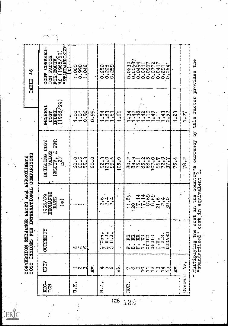
CONVERSION EXCHANGE RATES and APPROXIMATE

COST INDICES FOR INTERNATIONAL COMPARISONS

TABLE, 46

REG-

UNIV

CURRENCY

1968/69

BUILDING COST

GEWERAL

COST CONVERS-

ION

EXCHANGE

VALUE

-COST

ION FACTOR

RATE

(EQUIV. 2 PER

INDEX.

< FOR EQUIV .

( e )

r*2)'

(1968/69)

A-4' (1968/69)

akANDARDIZED'

(0

U.K.

11

60.0

-

1.00

1:000

2'

P-s

1-60.6

1.01

0.990

32

159.3

0.96

1..042

AV:.

6040

0.99:

N.

.4

Can.

2.6

92.3

1.54

0.250

5.

U.S.

2.4

123.0

1.83

.0.228

6') U.S.

-

2.4

99.6

1.61

0.259

Air,

-

_105.0

1.66

BU

R.

7F. FR

11.85.

80.2--

'

1.34

0.0630

8B. FR.

120

'

84.9

____1.42-

0.00587

910

N. KR

,

N. KR

17.14

17.14

75.1

85.2

-1-.-18---

1.42

0.0494

0.0411

11

GUILD

8.69

68.5

-

1.19

0.0967

12

GUILD

8.69

107,0

1.49

0.0772

13

T.U.

21.6

66.7

1.11

0.0417

14

U.S.

2.4

72.9

1.43

0.291-

1'5

DINARS

30.0

37.7

0.52

'0.0641

Av.

.

75.4

1.23

Overall Av.

78.2

1.27

*ralitiplying the cost in the country's

by this factor provides the

"standardized" cost in equivalent Z.

,Despite the scatter on the "basic" capital plot a very approximate'figure of£480 equivalent standardized per academic staff member was obtained.

The figures in table 45 demonstrate the variations due to building and,possibly, research referred to previously. In general recurrent expenditure lessremuneration per total staff pember is fairly constant across the regions being

about.Z1140 per total staff overall. The greater consistency. with total staff

,rather than academic staff is also apparent. The capital expenditure valuesdemonstrate the greater consistency :with academic staff but also emphasise the

caution that should be ex rcised in their interpretation. A study of the -"basic"

capital cost columns show that the value of £480 equivalent standardized per

academic staff memloer 1, give a rough guide in the absence of better data.

2.4.3. Converdion EXchange Rates and Approximate Coat Indices.

The indices set out in table 46.have been used throughout the discussionsof expenditure aboVe, and at the appropriate points in the preparation of theparameter values of section 4 of Chapter 3.

Building costs have been based on an approximate cost index of equivalent£ per square meter, deduced from average total staff salaries for the various

universities (which also reflect the individual nPture and relative cost, within

& region,-of these universities).

The cost indices are based on a more detailed review of. average salaries of

the various university groups and cost data generally. Cost conversion factors

,combine these indices with the'exchange rates for the country concerned toprovide,"standardized" data - referred to as £ equivalent "standardized" in the

text,for comparative purposes.

It is emphasized that although exchange rates are official. values the other

indices are only approximate and should be used with caution.

3. Further Data Observations on a Larger International Survey.

Two setd.ef-values of parameters, developed in the overall university model

of Chapter 2, haVe been incorporated in section 4 of that chapter. The aboveobservations based on the 15-university sample supplement the first seta In thispart further observations on the larger 80- university survey, which may not havebeen required for immediate use in the model evaluation, are presented. The

majority,Of these have particular relevance to the departmental academic, support,.

and administrative staff formulations in "both" the overall-model and the

departmental model (Chapter 3).

Part 3.3. of this section provides an evaluation of some additionalparameters utilized in the more conceptual departmental model of Chapter 3.

In the 80-university survey the data reduction is divided into fivegeographical groupings comprised as follows:

Group A.North America

United StatesCanada

Group BUnited Kingdom

EnglandWalesIreland

Group C,Scandinavia

DenmarkNorwaySwedenFinlandIceland

13o127

Group DPredominantly EEC

'GermanyAUstriaBelgiumFranceItalyNetherlandsLuxembourgSwitzerland

Group E"Other" European

SpainGreecePortugalMarkeyYugoslavia

3.1. Overall University Data

The following observations are derived from table 47.

Table 47. Overall. University Data

Item

.

Area Group

AllA B C D E

Iv. No. of Facultiesv. No. of Spec.

7.4 4.6 5.4 7.3 6.1 6.5

mats. Centres 9.8 7.0 3.4 5.2 5.3 6.2Inst. per Faculty

(Av.) 1.32 1.52 0.63 0.71 0.87 0.92

Av. No. Short Cours./year. 63 46 44 15

Av. Length of EachShort Cams. (days; 9.1 6.6 6.2 9.9 7.9 7.9

Av. No. Students/Short Course 76 25 45 42 43 48

'Relative intensityof effort index(1,) 16.0. 25.7 17.5 5.5 41.1 23.6

% B.F.T. Staff usedfor Hhort Courses(Approx.) 4.2 11.0 5.4 1.1 8.9 6.1

% Students in Resid.

(3) 27.3 36.8 14.1 18.2 21.9 24.2% Students in Resid. .

__.

(4) 24.3 36.8 2.0 13.4 21.9 18.5

% E.F.T. part-timeof total acad. -

staff 8.5 1.7 6., 22.1 21.3 13.0% E.F.T. part-time

of total acad.staff (4) 5.3 1.7 8.5 13.3 9.4 8.8

% Servicing from onefaculty to arztrier(Av.) 29 18 27 31-- 16

Servicing receivedby

Med. Sc. App.Sc./Tech.Soc.Soltd./Law Pure Sc. Educat. As.&Forest. Humanit.

Subj.Cless. Zl 22 23 17 48 56 15

% Students in Ind. 1.7 26.0(sandwich) (5) 2.1 0 9.o 7.3 0 5.5 26

Av. Hrs. visiting/4year/student . (all)

% Central_Adm. (byStaff) 54 56 44 34 39 44

Library: Tbtal Vol-umes (Av.) 977000 ' 166000 1088000 759000 310000 702000

Vblumes/Acad.Staff 1154 535 1300 898 1576 1060rota' periodicals/year 9976 2140 9752 7430 2180

eriodicals/Acad.Staff

F13.6 13.2 9.4, 5.6 106.:90

128

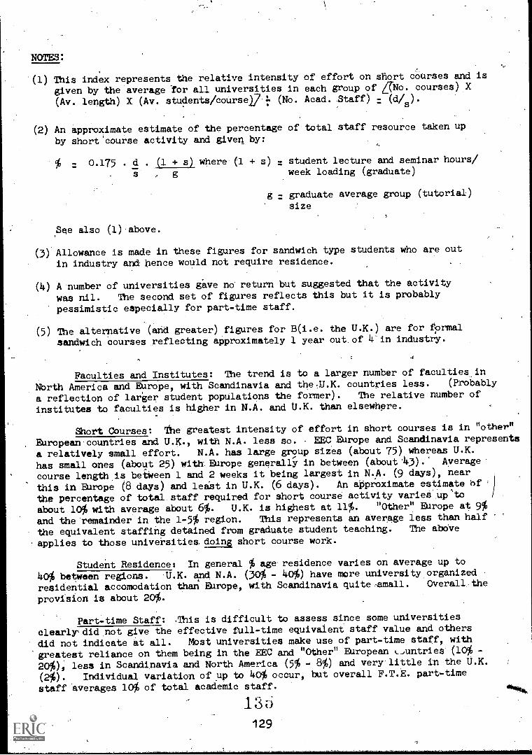
NOTES:

'(1) This index represents the relative intensity of effort on short courses and is

given by the average for all universities in each group of LTNo. courses) X

(Av. length) X (Av. students/course)7'= (No. Acad. Staff) (d/ ).

(2) An approximate estimate of the percentage of total staff resource taken up

by short'course activity and given by:

= 0.175 . d . (1 + s) where (1 + s) = student lecture and seminar hours/

. s g week loading (graduate)

g = graduate average group (tutorial)

size

See also (1).above.

(3) Allowance is made in these figures for sandwich type students who are out

in industry and hence would not require residence.

(4) A number of universities gave no return but suggested that the activity

was nil. The second set of figures reflects this but it is probably

pessimistic especially for part-time staff.

(5) The alternative (arid greater) figures for B(i.e. the U.K. ) are for Ormal

sandwich courses reflecting approximately 1 year out of 4 in industry.

Faculties and Institutes: The trend is to a larger number of faculties in

North America and EUrope, with Scandinavia and theU.K. countries less. (Probably

a reflection of larger student populations the former). The relative number of

institutes to faculties is higher in N.A. and U.K. than elsewhere.

Short Courses: the greatest intensity of effort in short courses is in "other"

European countries and U.K., with N.A. less so. EEC Europe and Scandinavia represents

a relatively small effort. N.A. has large group sizes (about 75) whereas U.K.

has small ones (about 25) with. Europe generally in between (about 43).' Average

course length is between 1 and 2 weeks it being largest in N.A. (9 days), near

this in Europe (8 days) and least in U.K. (6 days). An approximate estimate bf

the percentage of total staff required for short course activity varies up"to

about 10% with average about 6%. U.K. is highest at 11%. "Other" Europe at 9%

and the remainder in the 1-5% region. This represents an average less than half

the equivalent staffing detained from graduate student teaching. The above

applies to those universities doing short course work.

Student Residence: In general % age residence varies on average up to

40% between regions. U.K. and N.A. (30% - 40%) have more university organized

residential accomodation than Europe, with Scandinavia quite -small. Overall the

provision is about 20%.

Part-time Staff: This is difficult to assess since some universities

clearly,did,not give the effective full-time equivalent staff value and others

did not indicate at all. Most universities make use of part-time staff, with

'greatest reliance on them being in the EEC and "Other" European L,untries' (10% -

20%), less in Scandinavia and North America (5% - 8%) and very little in the O.K.

(2%). Individual variation of up to 40% occur, but overall F.T.E. part-time

staff averages 10% of total academic staff.

129

Service - .Teaching Between Faculties: Information was very poor on this andoften misinterpreted. Practically no university had estimated staff loading fromservice'teaching. Generally the information provided represented service receivedby students from staff of other faculties. The latter approXimated 23% overall,but ignoring smaller values (which- related to staff loading), all'the group valueslay between 22 and 29% with an average of 26%. Very soanty evidence suggestedthat staff loading for serving other faculties was about '6% 10% of totals academicstaff duties. The indications from subject classification show 15% - 23% servicingreceived by the more formal and established faculties (Humanities, Pure Science,Medicine, etc.) whilst the value is about 50% for the more vocational disciplines(Education;, Agriculture/Forestry).

Sandw ch Courses: Only universities in the U.K. ran full .:ormal sandwichprogrammes, i which the percentage of students in industry was 26% (i.e. oneyear in four).\ For other less formal programmes the group average was about 6%in induStryl thOugh rather greater in EEC Europe and "Other" Europe. Mbst ofthese programmes\appear-associated with Technology. Only:-five unive sitiesprovided a value \for average hours spent visiting students in industr , but theagvalues did not vary excessively, and averaged 48 hours. per year per s udent, based

a4

on visits per year to each student. This represents, very roughly about 0.1staff per sandwich student on academic teaching hours scales, or abou 0.03 staff.per sandwich student based on a 35 hour. working week. Thus full s wich coursescould imply up to 20% increase in staff.

Central Administration: This was based on staff numbers and d fines thepercentage of staff employed centrally, the remainder being distribut intofaculties, departments etc. Central administrative staff averages 5 % of totaladministrative support in N.A. and U.K. universities, and about 40%i for Europeanuniversities. The overall average of central/departmental or faculty administrative staff is 44%. There is considerable inter-regional variation. In terms ofcost these proportioni would be almost certainly higher asLhigher,grades are oftenrecruited centrally.

Library - Volumes and Periodicals:. There is considerable variation intotal volumes in libraries, from 166,000 in U.K. to 1,088,000 in Scandinavia.However values per academic staff member do not vary so widely. Overall thelatter is 1000 volumes/academic staff which could be regarded as the minimumdesirable. U.K. is about half this, although the sample is almost entirely"new" universities. "Other" EUropean and Scandinavian are 50% and 30% more,respectively. N.A. and "EEC" countries approach the average. *To some extentthese results reflect the methods of teaching adopted. There is again considerablevariation in the absolute 'totals of periodicals received annually, which vary from2,000 in the U.K. and "Other" European universities to 10,000 for N.A. andScandinavian. Again, the value of periodicals per academic staff member ismore uniform, varying from 5.6 to 13.6, in similar rankings to the totals.Clearly language and cost are vital factors. A rough desirable overall valuemight be about 10 periodicals per staff member, i.e. about 100 volumes perperiodical. . Clearly a full analysis must include such'factors as research,subject coverage and nature, special institutes, ability and dependence on differentlanguages etc. It must also include time-dependence as volume capacity is clearlya function of time fOr collections to grow to large size.

3.2. Faculty Data

The following observations relate to table 48.

Student Teaching: Overall there is few first. degree students providingteadhing support and where it'is undertaken, it is usdally limited to under 2 hours/week. There is considerably more higher degree student (graduate) teaching, and

13ti130

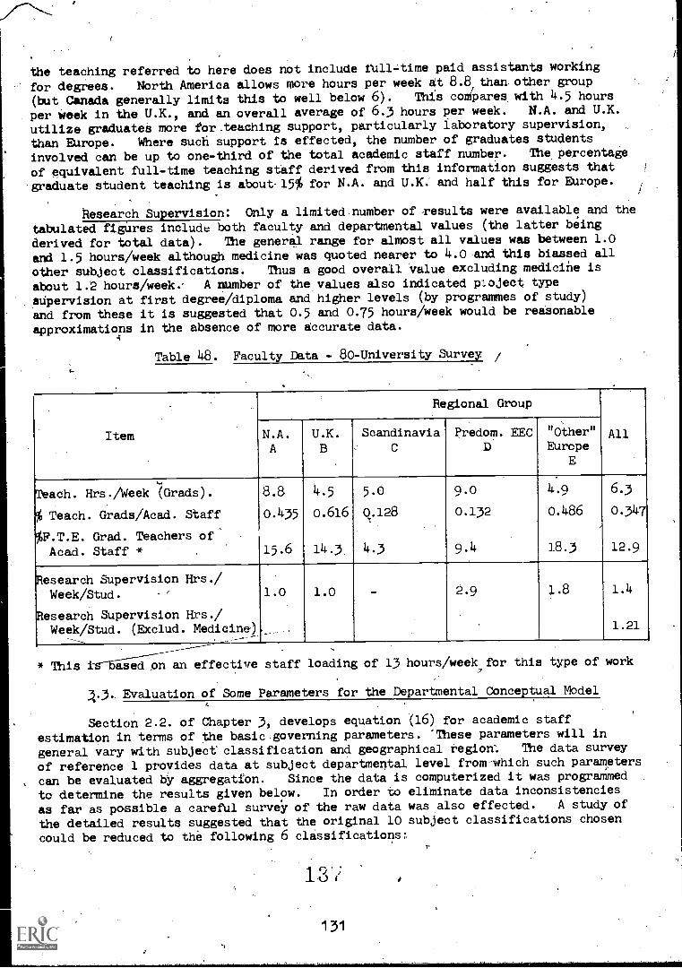
the teaching referred to here does not include full-time paid assistants working

for degrees. North America allows more hours per week at 8.8 than other group

(but Canada generally limits this to well below 6). This compares, with 4.5 hours

per week in the U.K., and an overall average of 6.3 hours per week. N.A. and U.K.

utilize graduates more for.teaching support, particularly laboratory supervision,

than EUrope. Where such support is effected, the number of graduates students

involved can be up to one-third of the total academic staff number. The percentage

of equivalent full-time teaching staff derived from this information suggests that

graduate student teaching is about 15% for N.A. and U.K. and half this for Europe.

Research Supervision: Only a limited.number of results were available and the

tabulated figures include both faculty and departmental values (the latter being

derived for total data). The general range for almOst all values was between 1.0

and 1.5 hours /week although medicine was quoted nearer to 4.0 and this biassed all

other subject classifications. Thus a good overall Value excluding medicine is

about 1.2 hours /week.' A number of the values also indicated project typesupervision at first degree/diploma and higher levels (by programmes of study)

and from these it is suggested that 0.5 and 0.75 hours/week would be reasonable

approximations in the absence of more accurate data.

Table 48. Faculty Data - 80-University Survey. /

Item

Regional Group

AllN.A.A

U.K.

BScandinavia

C

Predom. EECD

"Other"Europe

E

Teach. Hrs./Week (Grads). 8.8 4.5 5.0 9.0 4.9 6.3

% Teach. Grads/Acad. Staff 0.435 0.616 0.128 0.132 0.486 0.347

%F.T.E. Grad. Teachers ofAcad. Staff * 15.6 14.3 4.3 9.4 18.3 12.9

Research Supervision Hrs./Week/Stud. -' 1.0 1.0 - 2.9 1.8 1.4

Research Supervision Hrs./Week/Stud. (Exclud. Medicine) 1.21

--- _-

* This tS-Eiieii;n an effective staff loading of 13 hours/week for this type of work

1.3. Evaluation of Some Parameters for the Departmental Conceptual Model

Section 2.2. of Chapter 3, develops equation (16) for academic staff

estimation in terms of the basic governing parameters. 'These parameters will in

general vary with subject classification and geographical region: The data survey

of reference 1 provides data at subject departmental level from which such parameters

can be evaluated by aggregation. Since the data is computerized it was programmed

to determine the results given below. In order to eliminate data inconsistencies

as far as possible a careful survey of the raw data was also effected. A study of

the detailed results suggested that the original 10 subject classifications chosen

could be reduced to the following 6 classifications7'

131

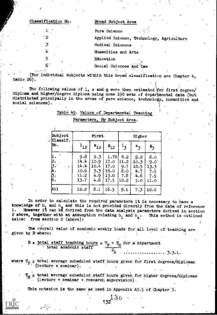
Classification No. Broad Subject Area

1 Pure Science

-2 Applied Science, Technology,, Agriculture

3 Medical Sciences

4 Humanities and Arts

5 Education

6 Soc:Lal Sciences:and Law

(Fbr individual subjects within this broad classification see Chapter 4,,

table 26).

The following values of 1, s and g were then estimated for first degree/diploma and higher/degree diploma using some 190 sets of depar ental data (butdistributed principally in the areas of pure science, technolo y, humanities andsocial sciences).

Table 49. Values of, Departmental Teaching

Parameters,'By Subject Area.

SubjectClassif.No.

First Higher

112

s12 g12

r

13 53

1. 9.8 9.3 1.70 6.2 9.2 8.o2. 14.4 10.9 17.0 11.2 10.3 9.03. 14.4 10.4 17.o 9.7 10.5 13.34. 10.6 5.3 16.0 8.o 4.7 7.55. 11.2 4.9 13.0 7.8 4.6 7.56. 13.7 4.8 17.5 10.2 5.0 11.0

All 12.2 8.1 16.5 9.1 7.3 10.0

In order to calculate the required parameters it is necessary to have aknowledge of hi and hs and this is not provided directly from the data of reference1. However it-can be derived from the data analysis parameters derived in section2 above, together with an assumption relating h1 and hs. This method is outlinedbelow: from section 2' (above):

The overall'value of academic weekly loads for all level of teaching aregiven by B where:.

B total staff teaching hours = Te + TH for a departmenttotal academic staff

DA 3.3.1.

where TF.

- tAal average scheduled staff hours given for first degrees/diplomas(lecture + seminar).

total average scheduled staff hours given for higher degrees/diplomas(lecture + seminar + research supervision)-

This notation is the same as used in Appendix A2.5 of Chapter 3.

13213 b

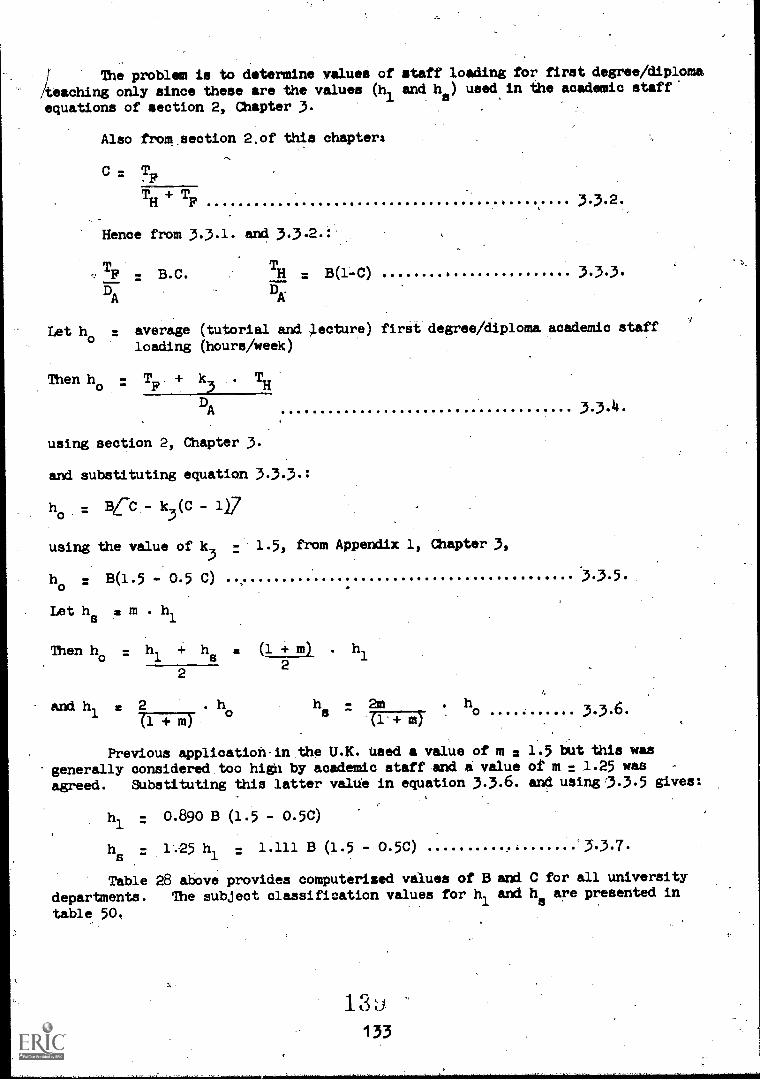
[ The problem is to determine values of staff loading for first degree/diploma

/teaching only since these are the values (h1 and he) used in the academic staffequations of section 2, Chapter 3.

Also from section 2.of this chapters

C TF

TH + TF3.3.

Hence from 3.3.1. and 3.3.2.:

TF : B.C. TH : B(1 -C) , 3.3.3.

DA

DA

Let ho _ average (tutorial and lecture) first degree/diploma academic staff

loading (hours /week)

Then ho

- TF. + k3

. TH

DA

using section 2, Chapter 3.

and substituting equation 3.3.3.:

ho

BCC - k3(C - 117

using the value of k3

- 1.5, from Appendix 1, Chapter

ho

B(1.5 - 0.5 C):

Let hs m

m . h1

Then ho

: + hs

= (1 + m) . hl1

22

3,

and h, - 2 . h h 2m ho

L

oO 4.111)

a-

3.3.4.

3.3.5.

3.3.6.

Previous application in the U.K. used a value of m s 1.5 but this wasgenerally considered too high by academic staff and a value of m 1.25 was -

agreed. Substituting this latter valtie in equation 3.3.6. and using' 3.3.5 gives:

hl - 0.890 B (1.5 - 0.50)

hs

1.25 hi. 1.111 B (1.5 - 0.5C)

Table 28 above provides computerised values of B and C for all university

departments. The subject classification values for h1 and 125 are presented in

table 50.

Table 50. Values for Average Staff Teaching

Loads per Week

SubjectClassif,No.

B Cho

h1

Hrs./Week

h8/s./Week

rr

1 8.081 0.684 9.36 8.33 10.402 10.12 0,780 11.25 10.00 12.503 8.14 0.762 9.12 8.12 10.154 9.52 0.772 10.6o 9.4 11.805 10.10 0.624 11.98 10.65 13.306 8.70 0.724 '9.89 8.80 11.00

i

All 9.16 0.728 10.40 9.26 11.58

Thus using these/Val4es of h1 andlis together with the valueS of s, 1 andg, above gives the subrbt classification parameters in the following table 51.

Table 51. Subject Classification Parameter Values

I

SubjectClassif.No.

1

1

Ac3/1a. .512/ h

a s/33/g . h

3h5

hT

1 1.18 0.75 0-0525 .0.1103 0.636 2.100 10.402 1.44 0.12 0.0513 0.0915 , 0.778 1.780 12.503 1.78 1.19. 0.0602 0.0778 0.669 1.292 10.154 1.13 0.85 0.0281 0.0530 0.752 1.887 11.805 0.96 0.73 0.0283 0.0461 0.760 1.629 13.306 1.56 1.16 0.0250 0.0413 0.744 1.652 11.00

All 1 1.32 0.98 0.0423 0.0630 0.747 1.491 11.58

where: u 1- 3/11

vi - s_ 3/g

si/gi

The above process can'he repealed to investigate geographical regionalvariation. HoweVer as subject classification appeared to be more significant,the exercise was limited to determining weighting factors for various geographicalregions bated on aggregated overall data. The resulting vallies are quoteddirectly in table.13 of Chapter 3.

1314

-TABLE 52

APPENDIX A3

Aggregated departmental

data by subject classification for all sample-universities

[CLASS

UNIV

1 2 3 4 5' 7 8 9

10

11 1314

15

(i )

TOTA

STAFF

(DT

)

171

226

304

112

333

201

610

370

'245

881

298

199

349.

(ii)

ITT5T-

ACAD.

rT:0''T,

STAFF

Tk;AG,d

0) )

HRS(T)

--4-

-87

852-

135

(1050)

143

15

78

1071

265

177

133

141

297

990

213

(2190)

160 .--1929

410

(3750)

135

438

132

512

188

2566

(iv)

-;ST.DEG

4:2ACH

HRS

(T

(v)

i

TOTAL

STUD.

(g)

(vi)

1ST

JLI:CT

ST-.71:,T

(ril),

TOTAL (vii)

W.00UREOT

EXPENDITURE

(MT).

,

(viii)

TOTAL

STAFF

REM. (V) tiA_

(ix)

AO. ST-.

RAM. (V

)(DT)

'207000

379000

443000

290000

912000

297000.

(569000

504000

322000

963000

367000

181000

580

804

--69O

528

1280

679

308

(1'100)

1929

(1980)

387

.

440

2114

541

960

1356

910

718

3469

1028

2109

3959

2161

.

2720

2515

1943

463

799

1055

718

274`

-

2627

610.

1198

3959

1311

2668

2475

'1328

438000

556000

1329000

363000

(123000)

485000

(1250000)

880000

508000

1682000

598000)

327000)

736000

._

...

-

290000

470000

1117000

335000

986000

353000

(100 9000

697000

416000

1358000

(526000

(262000

5570001490000

-,

IOTALAV

4299.

331

.

2376

19770'

183

1521

.12819

' 986

24374

1875

20085

1545

10379000

71 4000

8-367000

'

-644000

5924000.

456000

26

10

15,

(67)

6239

5352

29

(28)

679

_309

(11)

679

309

337:

277

320 A

143

277

320

(247000)

128000

(135000)

(202000)

114000

(10000)

174000

103000

(88000

365000

122000

I OTAL

AV

168

,56

13445

1016

339

.

999

333

934

311

7t0

247

,,..

510000

170000

,

....--....------

418000

139000

Llternative Comparative Table (Continued)(1)

---

CLA

SS

3:

Ui1

111

2 3 4-

6 8-

10

15

(i) 244

'

78

19

(763)

(29)

439

.

277

----

,---

---.

.(ii

)134

33

'

12

41720

,

267

145

(iii)

(1530)

\364

146

(698)

138

,

3553

.1797

-iv)

.93

18064

(197),

68

55-3

-'1260

(V)

1377

408

.

157

(3052)

223

2494

1839

(vi)

-1170

3'TO

14

1231

'

152

2494

1839

(vii.

).,

-604000

196000

'59000.

2123000

(75000)

867000

1167000

(viii

)493000

156000

'55000-

1928000

(60000)

730000.

7.06000

(ix)

384000

101000

45000

1225000

(47000)

536000

497000

OTAL

AV

.

1849

264

1028

147

8226

1175

6315

902'

9550

1364

7310

1044

5091000.

727000

4128000

590000

2835000

405000

4

'

2 5 7 811

1314

76 41

274

(21)

4642

79

38-

32

176

14

22 9

51

.(157)

20

19

185

-

(1w)

(35)

18.

96 14 0

-43

(39)

(20)

98

139

431

2898

-402

190

(395

)39

8

102

406 '0

217

-

113

(210

)351

189000

153000

(515000i

(42000)

87000

(920

00)

141000)

147000

13p000

425000

(34000)

7400O.-

(740

09(116000)

109000

121000

352000

A23000)

. =54000

(24000,)

'81000

TOTAL

AV

579 83

342 49

709

101

310

44

4854

693

1399

200

1219000 _

174000

1000000

143000

764000

109000 -

Alternative Comparative Table

(Continued)(2)

CLASS.

UNIV

(i)

(ii)

(iii)

(iv)

(v)

(vii)

(viii)

(ix)

55

48

30

1 ,

5.4

341

246

144000

13 5000:

1120100

61

98 Jo

84

1120

1025

883

820

235000

225000

213000

234

26

134

124

217

212

78000

75000

65000

4157

125

1500

879

1321

1032

479000

467000

422000

5267

232

3000

2425

3280

499

946000

842000

806000

6 ,7

123

214'1

100

196

48

-1596

31

1046

295

(2805)

202

(205)

433000

(509000)

386000

L1.54000

341000

440000

&182

108

981

544

1009

664

365000)

(333000)(228000)

9177

140

1680

1390

1696

1485

443000

402000

360000

11

322

271

2900

1770

2540

1647

799000

747000

708000

14

58

45

277

208

326

277

109000

100000

56000

15

176

125

1125

875

1438

1438

583000

432000

358000

TOT.

1808

1452.

14421

10317

15810

8481,

4978000.

4463C00

'001000.

Av.

164

132

1311

938

1437

771

453000

406000

364000

74

15

12

221

221

172

172

44000

39000

36000

5114

91

1700

1370

409

259

419000

357000

333000

8-

(78)

(56)

391

272

852

630

(199000)

(174000)(146000)

..-

TOT.

....I

207

159 -

2312

1863

1433

1061

662000

570000

515000

1

AV.

69

53

771

621

478

354

221000

190000

172000

Alte

rnat

ive

Comparative

Tab

le(Cont inued )

CLASS.

UNIV.

( i )

(ii)

(iii)

(iv)

(v)

)(vii)

(viii).

ix

.8

1 2 4 5' 8

11 14

1310

15

280

282013

9 710

220 20

1312

3(1.

.i.1

4,0)

167

4504

138

(158

)--

75

0 0 7519

12 68(131)

30

23 70

151

5200

223.

249

-, 85

0 0 16.

3900

152

2066 0

47000

23000

44000

9930

00(6

8000

)38

000

27000

23000

22000

41000

8200

00_(

5400

0)35000

21000

20000

20000

35000

661000

(420

00)1

27000.

19000

TOT.

AV.

379 54

291 .42

5221

746

2215

317

6001

857

4294

613

1240000

177000

1016000

145000

824000

1180

00 I

c 9.5 7 8 911

1215

43 45(66)

11,

152

5550

2229

42 9

120 48 32

140

152

185

(111

(1370

1250

256

140

140 47

.p13 525

600

192

409

830

1393

241

2233

675

489

409

800

605

241

1

1274

500

489

143000'

(113

000)

(155000)

29000

3790

00(163000)

159000

135000

(85000)

(138000)

28000

3710

00(145000)

126000

100000

(71000

(104000

26000

343000

(135000)

97000

TOT.

11V.

'422

60

302 43

.346

5.

495

1857 265

6270

896

4318

617

1141000

163000

1028000

147000

876000

125000

Alternative Comparative Table, ( Continued) (4)

CLASS.

(i)

OM

(iii)

. ,

(iv)

(v)

(vii)

(viii)

'x)

Di IV

.10

189

62

1:5-

230

./.45

220.

235000

162000

139000

294 -

78

'-°

317

678

4;2

229000

219000

203000

32,

-165-

2384

1310

1759

1348

605000

561000

489000

40

56

602

183'

496=

206

236000

229000

211000

5364

289

.2886

1965

3835

3182

1360000

092000

1003000

6.64

-

48

74

26

365

153

274000

229000

199000

738-

28

'203

,

173

598

598

103000

-

85000

77000

8119

79,

755

296

2020

1286

285000

234000

177000

931

27

284

.214.

226

208

94000

75000

Y70000

11

73'

57

522

338

687

510

171000

f163000

149000

12

;

190

134

552

487

(920)

(199

514000

423000

345000

13-

76

61

287

112

(2230)

.(2197

206000

182000

166000

14

71

,50

251

'

196

432

394

126000

103000

64000

-15

58

36

504

396

-

(865)

'(865)

303000

141000

112000

-1

TOT -

1566.

1170

9597

,6743

15456

11805

4741000

3898000

3404000,

AIT

119

84-

686

482:-:

1104

843

339000

278000

243000

Figures in brackets denote modifiedvalues of basic data tb provide

consistent figures.

References

1. CERI/OECD. University Informati n Survey 1968-69. CERI/W70.01.(0.E.C.D., Paris, JanuarY 1970.)

2. Legg, K.L.C., Note on an Approximate Analytical Approach to UniversityAcademie Planning. CERI/IM/69.06. nnex I. (0.E.C.D., Paris, 1969.)

3. Khan, A.G., and Fredrikson, B., A Preli nary Report on the CERI UniversityInforMation Survey 1968-69. CERI/1200. 8. (0.E.C.D., 'Paris, 1970.)

4. Legg, K.L.C., Brief Data Analysis on a 15-U versity International Sample.CERI/IM/71.27. (0.E.C.D., Paris, 1971.)

5. Legg, K.L.C., A Simple and Approximate Interne onal Data-Based UniversityOverall Resource Model. CER1/IM/73,28. (0.E. .D., Paris, 1971.)

6. Frederikson, B., University Information Survey 1 Report on DataCollection and Processing. CERI/TM/71.21. (0.E. Paris, 1971.)

-146

140