Legal Doctrine on Collegial Courts

Dimitri LandaDepartment of PoliticsNew York University

dimitri.landa@nyu.edu

Jeffrey R. Lax∗

Department of Political ScienceColumbia University

JRL2124@columbia.edu

November 24, 2008Forthcoming at Journal of Politics (2009)

Abstract

Appellate courts, which have the most control over legal doctrine, tend to operate throughcollegial (multi-member) decision-making. How does this collegiality affect their choice of legaldoctrine? Can decisions by appellate courts be expected to result in a meaningful collegialrule? How do such collegial rules differ from the rules of individual judges? We explore thesequestions and show that collegiality has important implications for the structure and contentof legal rules, as well as for the coherence, determinacy, and complexity of legal doctrine. Weprovide conditions for the occurrence of these doctrinal attributes in the output of collegialcourts. Finally, we consider the connection between the problems that arise in the collegialaggregation of a set of legal rules and those previously noted in the collegial application of asingle, fixed legal rule.

∗We thank Chris Berry, Ethan Bueno de Mesquita, David Epstein, John Ferejohn, Barry Friedman, Jake Gersen,Sandy Gordon, Cathy Hafer, John Kastellec, Lewis Kornhauser, Sarah Lawsky, Kelly Rader, and seminar participantsat the Harris School of Public Policy at the University of Chicago.

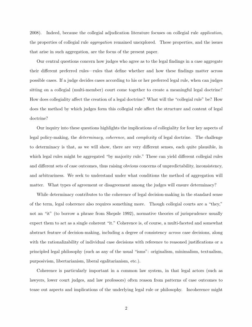
A lone judge deciding all cases herself could face a task overwhelming in practice, but straight-

forward in theory—she could simply decide all cases as she saw fit according to whatever rule she

thought correct. Judges on a collegial (multi-member) court, however, face further challenges that

inhere in collegiality itself.

One possible challenge is the application of existing legal rules. Kornhauser and Sager noted

back in 1986 that “traditional theories of adjudication are curiously incomplete,” in that they treat

judging only as a solitary act, and ignore the collegial nature of most appellate courts.1 They

showed that if the judges on a collegial court are applying a single, fixed legal rule, and if they

disagree over the legal sub-findings in a case, then it matters how they aggregate their judgments

over those sub-findings under the fixed legal rule. This result was later named the Doctrinal

Paradox, and it inspired a growing body of literature on collegial application of a fixed legal rule,

spanning legal theory, social choice theory, and deliberative democratic theory (e.g., Kornhauser

and Sager 1986, 1993, 2004; Kornhauser 1992a, b; Post and Salop 1992; Chapman 1998; List 2003;

List and Pettit 2002, 2005).

Appellate courts, however, do not only apply existing legal rules—they also create new rules

and modify old ones. They do not hear all cases themselves, but rather issue general rules and

instruct lower courts how to decide future cases. A lone appellate judge could do this by stating

her own preferred rule. Appellate courts, however, tend to be collegial courts. And appellate

judges can disagree far beyond whether the legal findings required by a given rule are met in a

given case.2 Specifically, they may disagree as to which of these legal findings should matter and

how much. That is, besides the challenge of collegial rule application, they also face a potentially

larger challenge, that of collegial rule creation. How can a collegial court choose a legal doctrine?

The analysis of doctrinal choice has recently emerged as a new frontier in the application of

social science tools to legal theory. Work in this vein has considered the implications of ideological

alignment, the role of precedent, hierarchical control, and biases towards litigants (e.g., Jacobi

and Tiller 2007, Tiller and Cross 2006; see also Bueno de Mesquita and Stephenson 2002). The

collegiality of doctrinal choice has received far less attention (but see Lax 2007 and Landa and Lax

1

2008). Indeed, because the collegial adjudication literature focuses on collegial rule application,

the properties of collegial rule aggregation remained unexplored. These properties, and the issues

that arise in such aggregation, are the focus of the present paper.

Our central questions concern how judges who agree as to the legal findings in a case aggregate

their different preferred rules—rules that define whether and how these findings matter across

possible cases. If a judge decides cases according to his or her preferred legal rule, when can judges

sitting on a collegial (multi-member) court come together to create a meaningful legal doctrine?

How does collegiality affect the creation of a legal doctrine? What will the “collegial rule” be? How

does the method by which judges form this collegial rule affect the structure and content of legal

doctrine?

Our inquiry into these questions highlights the implications of collegiality for four key aspects of

legal policy-making, the determinacy, coherence, and complexity of legal doctrine. The challenge

to determinacy is that, as we will show, there are very different senses, each quite plausible, in

which legal rules might be aggregated “by majority rule.” These can yield different collegial rules

and different sets of case outcomes, thus raising obvious concerns of unpredictability, inconsistency,

and arbitrariness. We seek to understand under what conditions the method of aggregation will

matter. What types of agreement or disagreement among the judges will ensure determinacy?

While determinacy contributes to the coherence of legal decision-making in the standard sense

of the term, legal coherence also requires something more. Though collegial courts are a “they,”

not an “it” (to borrow a phrase from Shepsle 1992), normative theories of jurisprudence usually

expect them to act as a single coherent “it.” Coherence is, of course, a multi-faceted and somewhat

abstract feature of decision-making, including a degree of consistency across case decisions, along

with the rationalizability of individual case decisions with reference to reasoned justifications or a

principled legal philosophy (such as any of the usual “isms”: originalism, minimalism, textualism,

purposivism, libertarianism, liberal egalitarianism, etc.).

Coherence is particularly important in a common law system, in that legal actors (such as

lawyers, lower court judges, and law professors) often reason from patterns of case outcomes to

tease out aspects and implications of the underlying legal rule or philosophy. Incoherence might

2

endanger communication with and the management of lower courts. As Fallon 2001 puts it, the

main judicial task is implementation of general principles, by constructing comprehensible rules

and tests. The ability of a collegial court to do this and speak in one, articulate voice may affect

the court’s efficacy within the judicial hierarchy, and is, at bottom, a central feature of legitimacy

and the rule of law (as justices themselves often acknowledge). We consider when collegial doctrine

will be coherent in this sense.

Finally, doctrinal complexity evokes explicitly the structure of a legal doctrine. Recent work

on the determinants of the legal doctrine has tied complexity to cases that have multiple issues

and the possibility of overlapping doctrines in a given case (Jacobi and Tiller 2007). Our analysis

considers the possible effects on complexity of collegiality itself.

We proceed as follows. After presenting some initial examples and highlighting our key results,

we introduce our basic assumptions and our formalization of legal cases and rules. Next, we discuss

collegial rules and analyze the methods by they which individual rules can be aggregated into a

collegial rule. The final formal section provides the results on the relationship between properties

of doctrinal aggregation and the doctrinal paradox. Formal proofs are in the Appendix, and

supplemental formal results are contained in an Online Appendix (available at ????).

Aggregating Rules

To foreshadow our results, we begin with examples of the phenomena we analyze:

(1) In Roth v. U.S., 354 U.S. 476 (1957), the U.S. Supreme Court placed obscenity outside

the protections of the First Amendment. Over the next ten years, the justices tried to define

“obscenity,” hearing over a dozen cases and issuing dozens of separate opinions (including Justice

Stewart’s famous “I know it when I see it” doctrine, in Jacobellis v. Ohio, 378 U.S. 184 (1964)).

In 1967, they gave up trying to state a formal definition, declaring it to be whatever five votes

said it was (Redrup v. New York, 386 U.S. 767). Under this “we know it when we see it” policy

(dropped six years and five new justices later), the justices themselves personally “Redrupped” the

evidence, sorting out at least 31 subsequent cases by summary disposition. They could sort out

cases by majority vote—but they were not able to articulate a workable standard for lower courts

that would accomplish the same result as majority votes case by case.

3

Any single justice among them could issue her own preferred rule so as to tell lower court judges

to “do as I would do.” Why could the justices not simply issue a rule that would amount to telling

lower courts judges to “do as we would do”?

(2) Imagine a lawyer trying a case before the Supreme Court, arguing that the proper rule

to apply to her type of case should consist of a specific set of legal determinations. As she runs

through this list of legal factors, she is pleased that for each and every factor at least five of the nine

justices nod in agreement. Even better, a justice who is usually the Court’s pivotal voter agrees

as to each and every factor. Yet when the decision is handed down, she loses her case. And, even

though each justice seems to reveal a preference for a simple, straightforward rule (albeit not the

same rule), the Court’s majority opinion instead establishes a complex balancing test.

The opposing verdicts in two 2005 establishment clause cases handed down the same day, Van

Orden v. Perry, 545 U.S. 677 and McCreary County v. ACLU of Kentucky, 545 U.S. 844, reveal

the tension between counting votes and counting the justices who support legal factors. Justice

Breyer’s differing votes permitted the state-sponsored display of the Ten Commendments in the

former but not the latter. The pivotal distinction for him was the historical circumstances behind

the displays—yet such an issue was not relevant to any majority of justices. That is, the case

outcomes are consistent with majorities voting case-by-case, while the outcome in Van Orden

stands in contrast to that indicated by majority positions on the legal factors that might compose

a legal rule for applying the establishment clause.

Another example is Kassel v. Consolidated Freightways, 450 U.S. 420 (1998), a dormant com-

merce clause case analyzed by Stearns (2000). Seven justices agreed that state’s attorneys should

be allowed to introduce novel evidence not considered by the Iowa legislature in support of the

statute in question. Five justices wished to apply the rational basis test. This combination of

factors would be necessary to sustain the statute—and it would seem that each factor did get the

nod from a majority of justices. However, only three justices agreed with both factors and so the

statute was struck. The problem is that different majorities agreed with each factor (in a plurality

opinion signed by four justices, with a concurring bloc of two, and a dissenting bloc of three).3

(3) Again, the Court is considering what the proper legal rule should be. This time, despite the

4

justices’ revealing strong differences as to what the proper legal rule should be, the Court announces

a relatively simple rule, which the lower courts then begin to apply—only to find the Court taking

further cases undercutting the initial rule and reversing the decisions below. An example here may

include the Rehnquist Court’s backtracking in Pierce County v. Guillen, 537 U.S. 129 (2003) from

their bold limitation of Congress’s commerce power in U.S. v. Lopez, 514 U.S. 549 (1995) and

U.S. v. Morrison, 529 U.S. 598 (2000) (see Berman 2004). Another example is the two-tier equal

protection framework (strict scrutiny vs. the rational basis test), which Justices Marshall and

Stevens each noted oversimplify the far more complex and nuanced actual pattern of decisions than

these sharply delineated tiers would suggest (see Stearns 2000, 15).

These examples point to phenomena that can arise in aggregating legal doctrines on collegial

courts. To see the basic structural elements of such aggregation, consider the so-called “Lemon

Test” formulated by the Supreme Court in Lemon v. Kurtzman, 403 U.S. 602 (1971). It is a three-

pronged test for a law to be constitutional under the Establishment Clause of the First Amendment:

it must have a legitimate secular purpose (LT1), must not have a primary effect of advancing or

inhibiting religion (LT2), and must not involve an excessive entanglement of government and religion

(LT3). But suppose that justices disagree over which of these prongs (or “factors”) are necessary for

constitutionality. How can a group of judges with different preferences over the inclusion of these

factors in an establishment-of-religion test aggregate their preferred legal doctrines into collegial

decisions?

The judges could simply decide each case one by one, without announcing a general rule—but

arguably the main task of appellate court judges is to aggregate their doctrinal preferences into

a single decision rule announce in their opinion, to be applied by lower courts and followed by

other actors. What rule could they issue? One presumptive interpretation is that they append a

rule that simply captures what would happen if they voted case by case. Alternatively, they could

append a rule that captures their preferences over each factor in turn (LT1, then LT2, and so on).

Or, they could pick a rule by an explicit vote over all possible general rules (formed by various

combinations of LT1 through LT3). Each of these options will indeed each yield a single composite

rule, but will they yield the same rule, matching collective decision making case by case?

5

The problem is that the various rule possibilities suggested above turn out to have systematic

differences. They may have sharply different substantive content and different implications for case

outcomes. The choice among them presents substantial complications that are of considerable

political importance. Specifically, the court’s task may be more complex and less feasible than may

have been previously recognized. The forms that collegial doctrines take may be due specifically

to collegiality, which can directly or indirectly—through judges’ attempts to manage it—affect

complexity and alter the structure of the legal policies we observe.

One of our conclusions, intimated in the various examples above, is an impossibility result :

“collegial” legal rules are different than individual legal rules, in that it might not be possible to

form the same type of rule for a court as a whole as any individual judge might have. That is, to

the extent that individual rules are each representative of coherent legal philosophies, it may not be

possible to construct a similarly principled collegial doctrine, at least not one that is representative

of the court in a majoritarian sense. Collegial courts thus face problems even beyond majoritarian

cycling (see Easterbrook 1982). Moreover, the legal rule that can “rationalize” the pattern of case-

by-case decisions by a collegial court often needs to be structurally different from and potentially

more complex than the preferred legal rules of the judges on the court (though collegiality can

sometimes smooth out complexity, making rules perhaps less nuanced). And, even when the court

can construct a coherent legal rule that captures the court’s preferences case by case—even a rule

that would be chosen by the majority over any other rule head to head—it may still be inconsistent

with the rule constructed from separate majority decisions on the elements comprising it that rule.

These findings mean that a collegial court can face a choice between adopting a rule that does not

comport structurally and/or substantively with the preferred rules of individual judges; abandoning

the pursuit of a single explicit rule (and issuing either overly narrow rulings or a multiplicity of

opinions); and adopting a rule that does not match how the collegial court wishes lower courts to

handle particular cases. (We set aside issues of compliance, but rather focus on what problems can

arise even if lower courts are faithful agents.) We analyze the conditions that determine when the

court cannot avoid having to make such a choice. We show, further, that there exists a fundamental

connection between some of the features that characterize the context of doctrinal aggregation and

6

those that characterize the aggregation of judgments under a fixed rule, particularly the structure

of the Doctrinal Paradox. Indeed, we provide necessary and sufficient conditions for a generalized

version of this paradox that operates on the level of doctrinal aggregation, as opposed to rule

application.

Modeling Cases and RulesThe aim of our model is to characterize some of the key substantive features of the corre-

spondence between collegial court output and the preferred rules of the individual judges, under

alternative modes of collective decision-making. Since our focus is the aggregation of rules, we iso-

late the issues involved by holding case findings as fixed and objective. The judges do not disagree

as to whether a given case meets the requirements of a given legal test (which would only make

collegial doctrine formation an even harder task). Rather, they differ as to what the elements of

the test should be.

Cases and Decisions

The two key conceptual elements in our model are cases and rules. Suppose there are k potential

legal dimensions, or “factors,” in a given issue area. A case is described in terms of these factors,

which may be thought of as a particular mix of both purely objective facts and intermediate legal

conclusions. Formally, a case can be represented by a list of values, indexed from 1 through k,

c = (c1, c2, ..., ci, ..., ck), indicating whether each of these k factors is present or absent in this case.

Let each value ci be 0 or 1, with the natural interpretation that ci = 1 means that factor i is

present in the case and ci = 0 that factor i is absent.4 For example, when there are two possible

factors (i.e., k = 2), one can identify four distinct possible cases: (0, 0), (0, 1), (1, 0), and (1, 1),

with the first factor being present in only the third and fourth cases, and the second factor only in

the second and fourth cases.

Rules

At the most general level, a legal rule ρ is a way of assigning an outcome (decision) to each

possible case, either “yes” (Y ) or “no” (N), ρ : c → {Y,N}. Because different rules can assign

different outcomes to a given case, the outcome of a case will depend both on the specifics of that

7

case and on the rule being applied. Let the set of decisions under the application of rule ρ to all

possible cases be the decision set of that rule. Below, we say that a rule ρ yields those outcomes.

So far, these definitions are compatible with any kind of structure connecting a description of cases

with outcomes.

The analytical structure that we impose on the legal rules in this paper invokes two key elements:

rule factors and the rule threshold. Let the list of rule factors that are considered (potentially)

relevant to a decision be represented by r = (r1, r2, ..., ri, ..., rk). We assume that each ri is either 0

or 1, with the interpretation that ri = 1 means that factor i is relevant under the rule in question,

and ri = 0 means that it is irrelevant. Consider, for example, a potential fourth Lemon Test prong:

the law must not affect one religion more than others (LT4). The original Lemon Test would deem

this prong irrelevant and so, explicitly reflecting its irrelevance, the test could be represented as

(1, 1, 1, 0).

A legal rule must also specify the logical relationship between these factors. For example, are

all of them necessary to reach a Y ? Are all of them individually sufficient? Are the factors treated

symmetrically? Or is there a more complex weighing of the factors?5 A key type of rule is a base

rule: base rules are rules that (1) identify which factors are relevant and (2) dictate a rule threshold

τ ∈ [0, k] setting the minimum number of factors needed for the decision Y rather than N .6

We say that a case factor ci contributes to meeting the threshold τ if and only if both ci = 1

(factor i exists in this case) and ri = 1 (that factor is relevant under this given rule). For example,

the Lemon Test threshold is three—all three factors must be found for constitutionality; further,

because the Lemon Test treats LT4 as irrelevant, the existence of the corresponding case factor

would not contribute to the case outcome.

Base rules can be compactly represented by a pair of the list of relevant rule factors r and the

threshold τ, (r; τ) (such that the case outcome is Y if and only if r · c ≥ τ). Our running example,

the Lemon Test, is representable as a base rule ((1, 1, 1), 3). If we wished to explicitly reject the

potential fourth prong to the test, we would add a dimension and have the rule ((1, 1, 1, 0), 3). Other

examples of possible base rules for k = 3 that a judge might prefer are ((1, 1, 0), 2), ((1, 1, 0), 1),

and ((0, 0, 1), 1). The first judge thinks ‘secular purpose’ and ‘no primary religious effect’ are both

8

necessary; the second judge thinks either is sufficient; and the third thinks ‘non-entanglement’ is

necessary and sufficient.

The case (1, 1, 0) will be decided as Y under rule ((1, 0, 1), 1)—the first case factor both exists

and is relevant, and this is sufficient under threshold τ = 1. The second factor exists in this case but

is irrelevant; the third factor is not present in this case but would be relevant if it were. However,

the decision in the case (1, 1, 0) would be N under the rules ((1, 0, 1), 2) or ((0, 0, 1), 1). Under the

former rule, only one existing factor is relevant and two are required; under the latter rule, only

one relevant factor is required, but neither of the factors that exist in this case is relevant. The

case (1, 0, 1) would receive decision Y under any of these rules.

Base rules include two prominent sub-categories of rules. Suppose there are m relevant factors

in the rule. At one extreme is the strict or conjunctive rule, one that requires each and every

relevant factor to exist to get a Y (τ = m). The Lemon Test is just such a test, in which all

prongs are necessary. Seemingly at the other extreme is a weak or disjunctive test, where the

presence of any one relevant factor is sufficient (τ = 1). Logically, however, these are structurally

equivalent: one could define a parallel Lemon Test as a strictly disjunctive test which yields a N

under the condition that any one of its prongs is missing.7 We call any purely conjunctive or purely

disjunctive test a simple rule, in that it takes the simplest and surely most common structure for

a logical rule.

A somewhat more complicated form of base rule is the intermediate rule, in which meeting the

threshold requires more than one factor but less than all m factors (1 < τ < m).8

Suppose, hypothetically, that the Lemon Test held that any 2 of its 3 prongs were sufficient.

In effect, then, instead of positing Y if and only if (LT1 and LT2 and LT3), that rule would be

described as positing Y if and only if ((LT1 and LT2) or (LT2 and LT3) or (LT1 and LT3)).

Despite this complication, such a rule can still be represented as a base rule - requiring a threshold

for symmetric factors, ((1, 1, 1), 2).

An example of an intermediate rule in action is the Winston test (Winston v. Mediafare Entm’t

Corp., 777 F.2d 78 (2d Cir. 1986) for pre-contractual liability, handed down by the Court of

Appeals for the 2nd Circuit. A subsequent 2nd Circuit decision, Ciaramella v. Reader’s Digest,

9

131 F.3d 320 (1997), provides the following instructive restatement and an elaboration of the test:9

This court has articulated four factors to guide the inquiry regarding whether parties

intended to be bound... (1) whether there has been an express reservation of the right

not to be bound in the absence of a signed writing; (2) whether there has been partial

performance of the contract; (3) whether all of the terms of the alleged contract have

been agreed upon; and (4) whether the agreement at issue is the type of contract that is

usually committed to writing. No single factor is decisive, but each provides significant

guidance.

The court goes on to cite Winston itself as a case wherein the agreement was found not binding

on appeal because “three of the four factors indicated that the parties had not intended to be

bound in the absence of a signed agreement.” In other words, one relevant factor was insufficient,

and not all relevant factors are necessary, making this an intermediate rule. Another example of an

intermediate test is that for differentiating a partner from an employee (Fenwick v. Unemployment

Comp. Comm., 133 NJL 295, 1945).

Finally, base rules can be distinguished from complex rules, which establish more complicated,

asymmetric relationships between factors, and so cannot be represented by a pair of factor list and

threshold. The disposition such a rule yields not only on how many factors are present but also

on which they are. For example, a complex rule might take the logical form A ∧ (B ∨ C), so that

the effects of C depend on which of the other two is present.

An interesting example is a recent Minnesota case, Lennartson v. Anoka-Hennepin, 662 N.W.2d

125 (2003). The Anoka County District Court cast the test for evaluating when a lawyer should be

disqualified (in a private sector case in which the lawyer’s firm has hired a lawyer who previously

represented the adverse party in the same matter) as a purely conjunctive test, with three factors

to be satisfied for allowing representation (if information is unlikely to be significant, the erection

of an ethical wall, and notice). The Court of Appeals reversed and remanded, declaring the proper

test to be a mixture of disjunctive and conjunctive tests (requiring insignificance or both an ethical

wall and notice), or, in our parlance, a complex rule. The Minnesota Supreme Court reversed again,

in favor of the original simple base rule. Another example of a complex rule is the “total takings”

10

rule of Lucas v. South Carolina Coastal Council, 505 U.S. 1003 (1992), declaring a governmental

regulation a compensable taking if (1) it destroys all economically viable use and either (2) the

restriction could not also have been imposed under the common law of nuisance or (3) the restriction

could not also have been imposed through the application of some legal principle related to the

title of the property.

Our primary analytical focus in this paper is on the properties of the collective aggregation of

judges’ individual rules. We thus largely focus on individual rules that are base rules (simple or

intermediate), so as to ask, inter alia, whether sets of case outcomes that represent the court’s

collegial decisions can be rationalized (induced) by a rule of the same structure and degree of

complexity—that is, whether the collegial rule will take the same form as the individual rules.10

This allows us to isolate collegiality as a potential source of doctrinal complexity (if the individual

rules were themselves complex, it would hardly be surprising that the collective rule were).11 It also

allows us to show that inherent properties of base rules are of particular substantive significance,

tying them directly to the necessary and sufficient conditions we establish for the appearance of a

generalized version of the Doctrinal Paradox.

We will speak of a judge’s preferred rule, yet for our purposes it is immaterial whether the

judge prefers a rule that, in turn, yields her preferred set of case outcomes, or rather prefers a set

of case outcomes that are then captured by her preferred rule. That is, it is immaterial whether

her most primitive preferences are over outcomes or over rules. It is also immaterial for the formal

analyses whether such preferences are derived from a higher legal philosophy or from the crudest

of ideological motives—either way, judges must express their preferences in terms of which cases

should win and which cases should lose. To say that a judge has an underlying preferred rule is,

in the end, to say that, whatever that judge’s preferences over the outcomes, they treat cases with

some minimal degree of consistency captured by the structure of the associated rule.

Outcome Sets

We begin by describing sets of case outcomes. Call the set of all possible cases C. The outcome

set associated with C specifies the outcome, Y or N , for each possible case. The following example

shows that not all outcome sets can be induced by a base rule.

11

Example 1. An outcome set:

case: (1,1,1) (1,1,0) (1,0,1) (0,1,1) (1,0,0) (0,1,0) (0,0,1) (0,0,0)outcome: Y Y Y Y Y N N N

It can be easily seen that there exists no simple or intermediate rule that yields this set of case

outcomes. Any rule with the threshold τ ≥ 2 fails for c = (1, 0, 0). To see that every rule with

τ = 1 fails as well, note that if the second rule factor, r2, is 1, then the outcome in (0, 1, 0) cannot

be N ; similarly, if the third rule factor, r3, is 1, then the outcome in (0, 0, 1) cannot be N either.

This leaves the rule ((1, 0, 0); 1), which in the case (0, 1, 1) yields N, contradicting the outcome Y

in that case provided in the table.

The property of being induced by a base rule is connected to another important property of

outcome sets captured in the following definition: an outcome set is monotonic if, whenever a given

case has outcome Y , any case with all the factors of the first case and at least one additional factor

also has outcome Y .

Example 1 clearly satisfies this property, but a combination of cases and outcomes that is

identical to it except for yielding N in any of the first three cases, (1, 1, 1), (1, 1, 0), or (1, 0, 1)

would not, since it would require assigning Y to the case (1, 0, 0).

Monotonicity of outcome sets ensures that the factual dimensions are not “coded” perversely

(i.e., such that, holding constant a legal rule, a case that more clearly fits a “liberal” outcome is less

likely to be decided that way than a case that fits that outcome less clearly). It may be thought of

as an important aspect of the coherence of judicial decision-making more generally. This intuition

is borne out by the following result:

Proposition 1. An outcome set can be induced by a base rule only if it is monotonic.

Thus, showing that an outcome set is coherent insofar as it can be induced by a base rule itself

means that that set satisfies another sense of coherence as well (viz., coherence as monotonicity).

However, this result cannot be strengthened to “if and only if”: not all monotonic outcome sets

can be induced by a base rule. As noted above, the outcome set in Example 1 is monotonic but

cannot be induced by a base rule.

12

Having set up a framework for thinking about rules and cases at the level of the individual

judge, we can now extend these concepts to analyze collegiality.

CollegialityIn all that follows, we assume that the court consists of n (odd) judges, J = {j1, ...jj , ..., jn},

who are making decisions either in cases or on rules that are then faithfully applied by lower courts.

Let ρ = (ρ1, ...ρj , ..., ρn) be a profile (list) of the judges’ most-preferred rules, one rule ρj = (rj ; τ j)

for each judge j. Judicial preferences, whether over case outcomes or the elements of rules, are

aggregated by simple majority rule.

Collegial Decisions

Given a set of judges and rules, a useful benchmark is provided by majority votes over case

decisions (each vote as induced by the judge’s preferred legal rule), leading to two definitions. The

collegial decision in case c is the decision preferred by the majority of judges given the judges’ rule

profile ρ. The collegial decision set is the outcome set formed by collegial decisions for each case

c ∈ C.

This collegial decision set will be “rational” in the following sense:

Proposition 2. The collegial decision set is monotonic.

Thus, aggregating by majority rule the preferred case decisions induced by judges’ preferred

base rules necessarily satisfies one important aspect of coherence. An implication of this proposition

is that in analyzing the properties of collegial decisions, we are effectively restricting our attention

to outcome sets that must already satisfy monotonicity. To the extent that we are interested in

ascertaining which collegial decision sets can be induced by a (simple or intermediate) base rule,

Propositions 1 and 2 establish that collegial rules satisfy a preliminary but non-trivial necessary

condition.

Given the benchmark represented by the collegial decision set, we next ask whether and how a

collegial court can achieve this outcome set short of voting case by case in all cases.

Collegial Rules

13

We begin with the following definitions. A legal rule ρ is the implicit collegial rule (ICR) of

the collegial decision set if ρ’s decision set is equal to the collegial decision set. A base ICR is a

rule (r; τ) such that its decision set is equal to the collegial decision set. A collegial decision set is

inducible by a base ICR if a base ICR exists for that decision set.

The outcomes induced by the ICR match the majority-preferred outcome in each case (as

determined by each judge’s individual rule). The following two examples provide an instructive

illustration. Unless noted otherwise, in all examples, the left-most column contains the ordered lists

r1, r2, and r3of rule factors for most preferred rules of each of the three judges; the second column

contains the thresholds for each of those rules, and the rest of the columns identify decisions under

each of the these rules for the cases specified in the top row. The bottom row identifies the collegial

decision in each case by majority vote.

Example 2.

rj τ j (1,1,1) (1,1,0) (1,0,1) (0,1,1) (1,0,0) (0,1,0) (0,0,1) (0,0,0)r1 = (1, 1, 0) 2 Y Y N N N N N Nr2 = (1, 0, 1) 2 Y N Y N N N N Nr3 = (0, 1, 1) 2 Y N N Y N N N N

collegial decision Y N N N N N N N

The collegial decision set is inducible by a base ICR ((1, 1, 1); 3), which is structurally equivalent

to the Lemon Test. Note an interesting implication of this example: while each of the three judges

preferred a two-prong simple conjunctive rule, the implicit collegial rule—though it is also simple

(and thus base)—is a more demanding three-prong test. Here, collegiality has the effect of ratcheting

up the demands of the effective decision-rule.

Moreover, the ICR is not the rule of any of the judges in this example. For this set of judges

to hand down a rule to match their desired outcomes, they would have to declare a rule that not

one judge among them would actually believe to be the correct legal rule. As we argue below, this

fact raises the issue of the extent to which collegial decision-making on the courts can be said to

produce results that are “representative” of the court.

The following example shows that collegiality can also change the kind of rule required to rep-

resent the collegial decision set, in that the aggregation of simple rules can require an intermediate

ICR, here ((1, 1, 1), 2). (Proposition 9 in the Online Appendix shows a necessary condition for the

14

ICR to be an intermediate rule.)

Example 3.

rj τ j (1,1,1) (1,1,0) (1,0,1) (0,1,1) (1,0,0) (0,1,0) (0,0,1) (0,0,0)r1 = (0, 1, 0) 1 Y Y N Y N Y N Nr2 = (1, 0, 0) 1 Y Y Y N Y N N Nr3 = (0, 0, 1) 1 Y N Y Y N N Y N

collegial decision Y Y Y Y N N N N

Since the ICR in this example is an intermediate rule, if the collegial court wants to issue a

simple rule, it must issue one that does not represent what the court itself would do in at least

some cases. Although, in this example, the effect of collegiality is to make the Court’s rule more

complex, it can also have the opposite effect:

Example 4.

Suppose each judge thinks a different one of the three factors is sufficient, with the remaining

pair jointly sufficient (e.g., Judge 1 requires either the first factor OR both of the second and third,

Judge 2 the second factor OR both the first and the third, and Judge 3 the third factor OR both

the first and the second). Each judge has a complex rule, but the collegial outcome set is induced

by the intermediate base rule ((1,1,1),2)):

case: (1,1,1) (1,1,0) (1,0,1) (0,1,1) (1,0,0) (0,1,0) (0,0,1) (0,0,0)outcome: Y Y Y Y N N N N

The next example provides support for another conclusion that is central for our analysis: the

aggregation of base rules may not be possible with either a simple rule or an intermediate rule, but

may instead require a complex rule:

Example 5.

rj τ j (1,1,1) (1,1,0) (1,0,1) (0,1,1) (1,0,0) (0,1,0) (0,0,1) (0,0,0)r1 = (1, 1, 0) 1 Y Y Y Y Y Y N Nr2 = (1, 0, 0) 1 Y Y Y N Y N N Nr3 = (1, 0, 1) 1 Y Y Y Y Y N Y N

collegial decision Y Y Y Y Y N N N

Note that the collegial decision set in this example is identical to the outcome set in Example

1. The discussion of that example, then, establishes that this collegial decision set is not inducible

by any base rule. This gives rise to the following result:

15

Proposition 3. Even when the collegial decision set is the result of the aggregation of individually

preferred decisions induced by a set of base rules, it may not be inducible by any base rule itself.

The rule that induces the collegial decision set in Example 5 would be a complex rule that

treat factors asymmetrically, mixing conjunction and disjunction: either the 1st or both the 2nd

and 3rd case factors are necessary and sufficient for the outcome Y. Note that this increase in the

complexity of the collegial rule is structural—it goes beyond an increase in the number of prongs

(as in Example 2), and moves beyond a shift from simple rule to intermediate rule (as in Example

3). This means that if the collegial court wishes to impose a base rule, it must choose one that

does not represent what the collegial court itself would decide in at least some subset of cases.

The non-existence of a base ICR in Example 5 and its existence in Examples 2 and 3 naturally

raise the question about the conditions that could account for this variation. One such condition

is on the number of dimensions. It is immediate to see that all 2-factor monotonic decisions sets

are inducible by a base rule. The ICR will be ((1, 1), 2), ((1, 0), 1), or ((0, 1), 1). Because, by

Proposition 2, collegial decision sets associated with judges described by base rules are always

monotonic, collegial courts will always yield decisions that are inducible by a base rule if there are

no more than two case factors of relevance. Are there conditions that apply to “larger” case spaces,

those with 3 or more potentially relevant factors?

In what follows, we consider two criteria for comparing rules, each providing such conditions.

One criterion compares rules by the direct patterns of their decisions, asking whether a given rule

“includes” all the Y outcomes of another rule: rule ρj decision-dominates rule ρd if, whenever ρd

yields the outcome Y , so does ρj . Example 5 provides an illustration of this property, in that the

first and third rules each decision-dominate the second, but not each other. Lemma 1 provides a

necessary and sufficient condition for decision-dominance in terms of the relationship between rule

factors and thresholds (see the proof of Proposition 6 or the Online Appendix).

Because decision-dominance is a transitive relation, it may be possible to order a number of

rules in relation to this condition. Say that a rule profile can be ordered by decision dominance if

for all pairs of rules (ρj and ρk), either ρj decision-dominates ρk, or ρk decision-dominates ρj , or

both. Thus, for example, it can be easily seen that the rule ((1, 1, 0); 1) strictly decision-dominates

16

((1, 1, 1); 2), which in turn strictly decision-dominates ((1, 1, 1); 3), and so the rule profile consisting

of these three rules can be (completely) ordered by decision-dominance. As our next result shows,

rule profiles that can be ordered in this fashion have an important property:

Proposition 4. The collegial decision set is inducible by a base rule if the profile of base legal rules

ρ can be ordered by decision dominance. The median rule in that ordering is the base ICR.

As Example 2 shows, however, the ordering by decision-dominance is only a sufficient and not

a necessary condition for the collegial decision set to have a base ICR. Moreover, the proof of

Proposition 4 shows that an even weaker condition than an orderable rule profile is sufficient. That

condition only requires that there exist one rule that decision-dominates half the remaining rules

and is in turn decision-dominated by all other rules. A rule which “splits” the remaining rules will

again be the base ICR.

Apart from decision-dominance, legal rules may also be compared to each other by their per-

missiveness. This property is determined by how “easy” it is for a given rule to reach a finding of

Y . Unlike decision dominance, permissiveness is based solely on a comparison of thresholds and

not on rule factors. A legal rule ρj is more permissive (less permissive) than a legal rule ρd if and

only if it has a smaller (larger) threshold. Legal rules ρj and ρd are equally permissive if they have

equal thresholds.

Because there is a certain trade-off between a value of the threshold and the number of factors

that the rule considers relevant (again see Lemma 1 in the proof of Proposition 6 or the Online

Appendix), the notion of rule permissiveness may be somewhat difficult to interpret. It does,

however, have an intuitive interpretation, holding constant factor values. In such a circumstance,

rule permissiveness may be thought of as a determinant of how “liberal” or “conservative” a rule

might be. For example, in the Lemon Test, where a finding of Y (constitutionality) is conservative, a

lower threshold (a more permissive rule) means a more conservative rule. Were a Y outcome instead

the liberal outcome, a higher threshold (lower permissiveness) would mean a more conservative rule.

The concept of permissiveness allows us to state our last result in this section, which identifies

a necessary property of base ICRs:

17

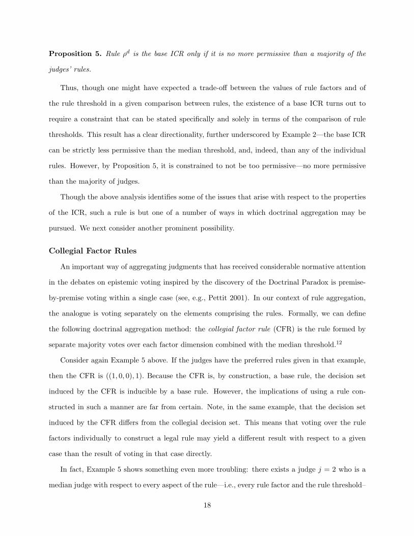
Proposition 5. Rule ρd is the base ICR only if it is no more permissive than a majority of the

judges’ rules.

Thus, though one might have expected a trade-off between the values of rule factors and of

the rule threshold in a given comparison between rules, the existence of a base ICR turns out to

require a constraint that can be stated specifically and solely in terms of the comparison of rule

thresholds. This result has a clear directionality, further underscored by Example 2—the base ICR

can be strictly less permissive than the median threshold, and, indeed, than any of the individual

rules. However, by Proposition 5, it is constrained to not be too permissive—no more permissive

than the majority of judges.

Though the above analysis identifies some of the issues that arise with respect to the properties

of the ICR, such a rule is but one of a number of ways in which doctrinal aggregation may be

pursued. We next consider another prominent possibility.

Collegial Factor Rules

An important way of aggregating judgments that has received considerable normative attention

in the debates on epistemic voting inspired by the discovery of the Doctrinal Paradox is premise-

by-premise voting within a single case (see, e.g., Pettit 2001). In our context of rule aggregation,

the analogue is voting separately on the elements comprising the rules. Formally, we can define

the following doctrinal aggregation method: the collegial factor rule (CFR) is the rule formed by

separate majority votes over each factor dimension combined with the median threshold.12

Consider again Example 5 above. If the judges have the preferred rules given in that example,

then the CFR is ((1, 0, 0), 1). Because the CFR is, by construction, a base rule, the decision set

induced by the CFR is inducible by a base rule. However, the implications of using a rule con-

structed in such a manner are far from certain. Note, in the same example, that the decision set

induced by the CFR differs from the collegial decision set. This means that voting over the rule

factors individually to construct a legal rule may yield a different result with respect to a given

case than the result of voting in that case directly.

In fact, Example 5 shows something even more troubling: there exists a judge j = 2 who is a

median judge with respect to every aspect of the rule—i.e., every rule factor and the rule threshold–

18

and thus, j’s preferred rule is the CFR. Despite this, judge j can still end up in the minority with

respect to some cases (here, in the case c = (0, 1, 1)). This is the problem captured in our second

introductory anecdote: the lawyer with case (0, 1, 1) and arguing for rule (1, 0, 0) will get judge 2’s

vote factor-by-factor along with a majority of judges factor-by-factor, but if they decide this case

by majority vote, she will lose.

Given the non-existence of a base ICR in Example 5, it is natural to ask whether and how

the two phenomena are linked. To begin with, does the coherence of collegial decision-making

associated with the existence of a base ICR prevent the kind of incoherence suggested by the gap

between the collegial decision set and the decision set induced by the CFR?

Consider Example 2 above, in which the collegial decision set does have a corresponding base

ICR ((1, 1, 1), 3). However, the CFR in that example is ((1, 1, 1), 2), which produces different judg-

ments in cases (1, 1, 0), (1, 0, 1), and (0, 1, 1). (Note that neither the ICR nor the CFR matches the

individual rules of any of the judges on the court.) Thus, the existence of a base ICR does not imply

that the collegial decision set is inducible by the CFR. That is, the ICR need not be identical to

the CFR. (The relationship between them will be crucial in our analysis below of the Generalized

Doctrinal Paradox.)

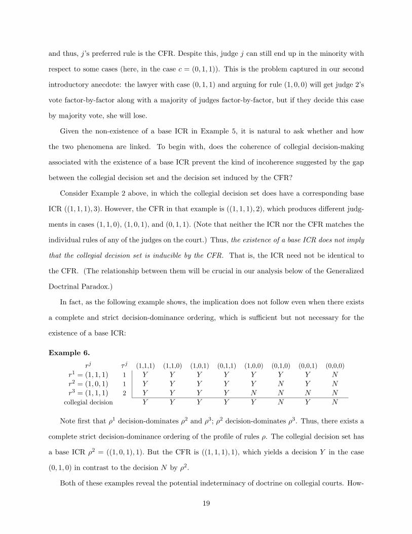
In fact, as the following example shows, the implication does not follow even when there exists

a complete and strict decision-dominance ordering, which is sufficient but not necessary for the

existence of a base ICR:

Example 6.

rj τ j (1,1,1) (1,1,0) (1,0,1) (0,1,1) (1,0,0) (0,1,0) (0,0,1) (0,0,0)r1 = (1, 1, 1) 1 Y Y Y Y Y Y Y Nr2 = (1, 0, 1) 1 Y Y Y Y Y N Y Nr3 = (1, 1, 1) 2 Y Y Y Y N N N N

collegial decision Y Y Y Y Y N Y N

Note first that ρ1 decision-dominates ρ2 and ρ3; ρ2 decision-dominates ρ3. Thus, there exists a

complete strict decision-dominance ordering of the profile of rules ρ. The collegial decision set has

a base ICR ρ2 = ((1, 0, 1), 1). But the CFR is ((1, 1, 1), 1), which yields a decision Y in the case

(0, 1, 0) in contrast to the decision N by ρ2.

Both of these examples reveal the potential indeterminacy of doctrine on collegial courts. How-

19

ever, given a decision-dominance ordering, one additional condition, invoking rule permissiveness

as defined above, is sufficient to prevent this from occurring:

Proposition 6. Suppose that legal rules in profile ρ can be ordered by decision-dominance and are

equally permissive. Then, (a) a rule ρj is a CFR if and only if it is a base ICR, and (b) both the

CFR and the ICR coincide with the preferred rule of the median judge in the decision-dominance

ordering.

Thus, although the existence of a base ICR does not, generally, imply that it matches the CFR,

these rules are identical under the particular conditions we invoked above.13

The Collegial Rule Choice

The next part of our formal analysis explores judges’ voting directly over rules. Our predictive

concept for the outcomes of rule choice is the majority core in rule choice—the set of rules that

would not be defeated under majority rule by any possible rule in a pair-wise comparison by the

members of the court. To say something meaningful about the content of the majority core in rule

choice, we need to introduce judges’ utility functions. There are many possible choices for what

those functions should look like. Though the choice among these will have effects for the conditions

under which the majority core may be expected to be non-empty, our primary focus in this section

is not on the characterization of those conditions (that is, no doubt, an important issue in and of

itself, but one that lies outside the scope and the aim of the present paper), but on the properties

of the majority core prediction, when that prediction can be made. Thus, in the remainder of this

subsection, we assume what is possibly the simplest form of the utility function that generates a

non-empty core under the conditions on rule profiles introduced above. This function treats the

cases symmetrically, giving a judge the same positive payoff in all case outcome in which she “wins”

(the case outcome matches her preferred decision), and the same negative or zero value in all cases

in which she “loses.” In other words, it simply counts case victories.

Our next result shows that a sufficient condition for the existence of a base ICR ensures that

that rule is in the majority core in rule choice:

Proposition 7. Suppose that legal rules in profile ρ can be ordered by decision-dominance. Then

20

the ICR must be in the majority core of rule choice, while the CFR need not be.

Because the CFR may differ from the ICR even if the rule profile can be ordered by decision-

dominance (Example 6), and because the ICR is in the majority core of rule choice when the

rule profile can be ordered by decision-dominance (Proposition 7), it follows that under the same

dominance condition the CFR may differ from the majority core rule. Put differently, even when a

base ICR exists and would be chosen by the majority rule on the court when compared to any other

legal rule, it may be inconsistent with the rule constructed from separate majority decisions on the

elements composing it. This reveals a key problem in doctrinal aggregation and raises questions

of indeterminacy. However, when we also require that all judges’ rules be equally permissive, the

CFR must be in the majority core:

Corollary 1. Suppose that legal rules in profile ρ can be ordered by decision-dominance and are

equally permissive. Then the CFR coincides with the ICR and is in the majority core.

The Generalized Doctrinal Paradox

The final part of our formal analysis concerns the relationship between the framework of doc-

trinal aggregation and the analytical structure of Kornhauser and Sager’s Doctrinal Paradox. The

essence of the Doctrinal Paradox is the possible disparity between the outcomes of using majority

votes (1) over individual factor decisions which are then aggregated to yield an input into a legal

rule or (2) over the preferred judgments of each judge, each individually applying that legal rule.

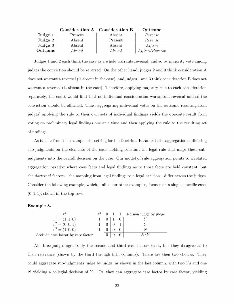
The following example (Kornhauser and Sager 1986, 115) provides an illustration. Suppose that

a criminal appeals her conviction on two grounds (considerations A and B, respectively), either of

which would be sufficient and at least one of which would be necessary to reverse the conviction.

(That is, the underlying rule used by the judges is ((1, 1), 1).) The court is to decide by majority

rule, and the individual judges comprising it arrive at the following evaluations of the relevant

issues:

Example 7.

21

Consideration A Consideration B OutcomeJudge 1 Present Absent ReverseJudge 2 Absent Present ReverseJudge 3 Absent Absent AffirmOutcome Absent Absent Affirm/Reverse

Judges 1 and 2 each think the case as a whole warrants reversal, and so by majority vote among

judges the conviction should be reversed. On the other hand, judges 2 and 3 think consideration A

does not warrant a reversal (is absent in the case), and judges 1 and 3 think consideration B does not

warrant a reversal (is absent in the case). Therefore, applying majority rule to each consideration

separately, the court would find that no individual consideration warrants a reversal and so the

conviction should be affirmed. Thus, aggregating individual votes on the outcome resulting from

judges’ applying the rule to their own sets of individual findings yields the opposite result from

voting on preliminary legal findings one at a time and then applying the rule to the resulting set

of findings.

As is clear from this example, the setting for the Doctrinal Paradox is the aggregation of differing

sub-judgments on the elements of the case, holding constant the legal rule that maps these sub-

judgments into the overall decision on the case. Our model of rule aggregation points to a related

aggregation paradox where case facts and legal findings as to those facts are held constant, but

the doctrinal factors—the mapping from legal findings to a legal decision—differ across the judges.

Consider the following example, which, unlike our other examples, focuses on a single, specific case,

(0, 1, 1), shown in the top row.

Example 8.

rj τ j 0 1 1 decision judge by judger1 = (1, 1, 0) 1 0 1 0 Yr2 = (0, 0, 1) 1 0 0 1 Yr3 = (1, 0, 0) 1 0 0 0 N

decision case factor by case factor 0 0 0 N\Y

All three judges agree only the second and third case factors exist, but they disagree as to

their relevance (shown by the third through fifth columns). There are then two choices. They

could aggregate sub-judgments judge by judge, as shown in the last column, with two Y s and one

N yielding a collegial decision of Y . Or, they can aggregate case factor by case factor, yielding

22

the bottom row with the vector (0, 0, 0) of factor judgments, leading to a decision of N under the

collegial factor rule ((1, 0, 0), 1), and so contradicting judge-by-judge aggregation.

This example has an analytical structure closely related to that of the Doctrinal Paradox, as

can be seen in the following definition of an analytical object that subsumes both of the above

examples. For each judge j and for each case c, let f j,c be a vector of case findings—these are case-

specific values that in our model correspond to case factors of the case c, (c1, c2, ..., ck), and in the

Kornhauser-Sager example above correspond to the vectors of “present” and “absent.” Let R and

F c be the aggregate vectors of rule factors and case findings, respectively (by majority votes over

each), and T be the aggregate rule threshold (the median threshold). Note that, consistent with

our assumptions above, F c = f j,c for all j in our model (our judges agree as to the case findings),

while R = rj for all j in Kornhauser and Sager’s analysis (their judges agree as to the rule). Say

that a rule profile ρ manifests a Generalized Doctrinal Paradox if there exists a case c such that

either R ·F c ≥ T but the collegial decision in the case is N or R ·F c < T but the collegial decision

in the case is Y—that is, if factor-by-factor aggregation differs from judge-by-judge aggregation.14

The following result characterizes the analytical connection between the subtleties of judgement

aggregation in our model of doctrinal aggregation and the Generalized Doctrinal Paradox:

Proposition 8. Let all judges agree as to which case factors are present (that is, ∀j ∈ J , ∀c ∈ C:

F c = f j,c). Then, given a rule profile ρ, (a) If a base ICR does not exist, then ρ manifests the

Generalized Doctrinal Paradox; (b) If a base ICR exists but is not equivalent to the CFR, then ρ

manifests the Generalized Doctrinal Paradox, and the cases where these rules conflict are the very

cases that give rise to the Generalized Doctrinal Paradox; (c) If a base ICR exists and is equivalent

to the CFR, ρ will not manifest the Generalized Doctrinal Paradox.

Part (a) of Proposition 8 shows, then, that the non-existence of a base ICR is sufficient to guar-

antee that ρ will manifest the Generalized Doctrinal Paradox. Part (b) of Proposition 8 implies that

decision-dominance (which, by Proposition 4 is sufficient to guarantee the existence of a base ICR) is

not sufficient to prevent the Generalized Doctrinal Paradox. Nor is decision dominance necessary

to prevent the Generalized Doctrinal Paradox. The profile (((1, 1, 0), 1);((1, 0, 1), 1);((0, 1, 1), 1))

cannot be decision-dominance ordered, but has base ICR ((1, 1, 1), 1), which is also the CFR for

23

this profile. It follows immediately that ρ does not manifest the Generalized Doctrinal Paradox.

Although decision dominance is, therefore, neither necessary nor sufficient to prevent the Gen-

eralized Doctrinal Paradox, one implication of Proposition 6 is that the combination of decision-

dominance and equal permissiveness of legal rules is indeed sufficient for that purpose. As Propo-

sition 6 (b) shows, when those two conditions obtain, the CFR and the base ICR coincide with the

preferred rule of the median judge in the decision-dominance ordering. Indeed, we can state the

following necessary and sufficient condition directly in terms of the identity of the median judge:

Corollary 2. Suppose a rule profile ρ that can be ordered by decision-dominance. Then ρ does not

manifest the Generalized Doctrinal Paradox if and only if the factor-by-factor median judge is also

a median judge in the decision-dominance ordering of ρ.

Thus, when the factor-by-factor median judge is not the median judge in the decision-dominance

ordering of ρ, ρ manifests the Generalized Doctrinal Paradox (because the CFR does not equal the

ICR). Indeed, it is noteworthy that the cases that give rise to the paradox may occur both when

the factor-by-factor median judge loses in the majority rule aggregation of overall judgments (as

in case (0, 1, 1) in Example 8) and when there exists a median judge in the decision-dominance

ordered profile (and desired case outcomes) who loses in the factor-by-factor aggregation (as in

case (0, 1, 0) in Example 6).

In effect, this shows that no matter how we define a median judge, by the outcomes of cases

or by the individual doctrinal requirements, the existence thereof does not prevent the Generalized

Doctrinal Paradox. Consistency and predictability are still at risk either way.

Discussion

In an influential essay, Judge Easterbrook (1982, 815) argued that, while it may be reasonable

to expect an individual judge’s preferred rule to be one that corresponds to a minimally principled

legal philosophy, social choice-theoretic problems of collective cycling over rules (exemplified by

Condorcet’s Paradox) imply that it is inappropriate to criticize a collegial court for the lack of

coherence, so defined.15 Our analysis offers what may be seen as a complementary view that does

not rely on the existence of preference cycles or on the court’s failures to check them.

24

One aspect of this view is the Generalized Doctrinal Paradox, which extends Kornhauser and

Sager’s key finding from the domain of rule application to the domain of doctrinal aggregation.

Another aspect derives from our results on the base-rule rationalizability of collegial decision sets,

the lack of which is shown to be a necessary condition for the existence of the Generalized Doc-

trinal Paradox, but which also gives rise to a somewhat distinct set of concerns. Suppose that

each individual judge’s rule reflects a consistent jurisprudence of some sort.16 The aggregation of

individual judges’ judgments may result in an object—either a rule or a set of case decisions that

may be explainable by some rule—that is structurally distinct from the individual judges’ rules

and their case implications. Though some set of philosophical principles may indeed be found to

support this amalgamated product, there is no reason to believe that such set must exist; at the

very least, the judges may have to go outside their collective set of such principles to find it, and

the resulting rule loses the presumption of principled justification that we might associate with

the opinions of judges taken as individuals.17 Because opinions are rarely if ever complete and un-

equivocal descriptions that can be enforced or implemented without interpretation by legal agents

downstream, the absence of a clear and consistent connection to a background legal philosophy

may make it more difficult to predict what the collegial high Court will do, undermine consistency

of judgments across lower courts, reduce persuasive power (Ferejohn and Pasquino 2002), and,

consequently, reduce judicial legitimacy.

Note that the problems of aggregation we have demonstrated exist no matter how principled

the judges are, and given the most optimistic assumptions about their motives. This conclusion

is troublesome, given that much legal scholarship seeks to attack or defend the output of collegial

courts in terms of jurisprudential consistency. Given the collegial nature of higher courts, the

normative account of law as “integrity” advanced by Dworkin (1986) may simply be outside of

logical possibility.18

The framework and results of this paper also allow us to address some of the key issues involved

in the differing versions of stare decisis—dependent on whether subsequent judges are or should be

bound by the reasons provided by their predecessors, the rules stated by them, or the case outcomes

they handed down (see Kornhauser 1992a). First, note that if rules are derived from previous case

25

outcomes, then, barring changes on the court, the result will be the collegial decision set. As we

show above, this set may or may not be supportable by a single implicit base rule. Alternatively,

we might consider the precedent set by the determination of the proper role of a single legal factor.

In this fashion, the precedent-respecting court may be seen as constructing a rule by decisions on

rule factors. This way of proceeding would lead to the collegial factor rule, which, as we show

above, may systematically differ from the implicit collegial rule, even when the latter may be in

the majority core of rule choice.

Our results in relation to these focal modes of stare decisis raise concerns about the compatibility

of stare decisis and a “coherence” or “integrity” account of legal adjudication. A rule might be

considered effective and stable only if it is supportable upon majoritarian appellate review. When

the implicit collegial rule is announced by the court, then we know for a fact that settlement is final

and the law settled. If not, then we might expect appeals that will undercut the collegial court’s

announced rule.

Even if the collegial court consistently uses one particular aggregation method rather than

others, the concerns that we associate with (in-)determinacy are still present. When there exist

disagreements between the collegial factor rule, the implicit collegial rule, and the majority core

rule, these disagreements can be implicitly revealed by dissenting and concurrent opinions. This

would suggest to lower courts or other actors that they can push to find the “right” case, one

that could get a majority vote on the high court inconsistent with the court’s previous stated

opinion. In effect, it sends a signal that there may be “wiggle room” in the decision, that other

cases may yield a winning combination of factors. To what extent this is desirable turns on whether

we associate greater value with encouraging the development of the law or with avoiding giving

the encouragement to other actors to push the “doctrinal envelope” (think, desegregation cases).

The justices might indeed agree up front how to aggregate their rules when writing an opinion,

but one may reasonably doubt their commitment to sticking with that opinion in a future case

for which there are five or more votes to rule otherwise. Finally, the divergence between implicit

collegial rule, the collegial factor rule, and the majority core may be thought to create a sense that

courts’ decisions as a whole (across various issues) are substantively arbitrary rather than reasoned

26

and “necessary.” The general consequence is to further undermine the persuasive power and the

perceived legitimacy of the court.

Second-order preferences over rules

Consistent with much of the political science literature on the courts, we assumed in the preced-

ing that judges’ preferences over legal rules are induced entirely by substantive concerns associated

with particular cases. However, the recognition of effects of collegiality that we analyze in this

paper may also lead judges to develop second-order preferences over the content and structure of

rules that would directly reflect valuing coherence. If judges are concerned with coherence, espe-

cially in the opinions bearing their names, they might prefer to announce simpler (base) rules in a

given case (consider the strict scrutiny/rational basis simplification discussed in the introduction)

and then later take up further cases to promulgate other rules that would, on their own, call for a

different disposition in the initial case. Proceeding in this way, the court might develop a complex

doctrine, one not necessarily coherent taken as a whole (takings law seems to be a favorite target

for such accusations). In this sense, our results should not be taken to imply that complexity comes

only in the form of explicitly complex rules. Rather, it can arise in the form of what would amount

to a complex—and possibly incoherent—doctrine spanning different rulings.

The pressures we note herein might therefore not be manifested in observable opinion outputs—

after all, we do not get to observe the individual rules preferred by the judges in isolation without

the pressures of collegiality—but rather play a role behind the scenes in how law is produced,

given the “costs” of collegiality. Judges have at their disposal a range of coping mechanisms

for dealing with the various pressures and problems that we identify in this paper. None of these

mechanisms is “free”—each comes at its own cost, or trade-off. One can think of these mechanisms

as belonging to a spectrum defined by how strongly the judges feel about the particular substantive

or ideological concern represented by a given case relative to the value they place on coherence and

other collective goods. At one end of that spectrum are direct concessions, accommodations, and

bargaining between coalition members who are concerned with the collective good of the collegial

output but disagree over its precise content.19 At the other end are concurrences (both regular

concurrences, written along with joining the majority opinion, and special concurrences, which

27

only add a vote for the majority outcome), which may indicate judges’ relative unwillingness to

compromise on a majority opinion/collegial rule and their relative readiness to give it up for the

sake of issuing relatively unconstrained individual pronouncements (and a judgment of the Court).

This could force lower courts to attempt to count votes behind different sections of the opinions

and behind different arguments or rule factors, which could lead again to the implicit collegial rule

“de facto” if not “de jure.”20

Between these ends of the spectrum lie several legal practices that have been the focus of recent

attention in legal theory. One such practice is intentional vagueness in the court opinion and

postponement of a clear statement of the general rule behind it (see Vanberg and Staton 2007). A

closely related practice, also giving up on a determinate rule, is the endorsement of an indeterminate

standard (Kaplow 1992, Sullivan 1992, Posner 1997, Schauer 1991, Fallon 2001, Jacobi and Tiller

2007). Still another relevant and somewhat more distinct practice is the narrow casting of appellate

case decisions, which, Sunstein (1993) argues, is a desirable feature of decision-making in a morally

pluralist society, in which “completely theorized agreement” on the principled support for a legal

doctrine may be difficult, if not impossible, to obtain. Of course, the justices could just avoid

deciding at all. (As Stearns 2000 argues, doctrines such as standing and justiciability may enable

the justices to duck troublesome cases, thereby avoiding cycling over rules, public incoherence, and

manipulation by outside agents.) Each of these mechanisms may serve to stabilize law and policy.

One of the implications of our arguments is that their relative prevalence may be associated with

particular properties of collegial adjudication and the presence of features of disagreement among

the members of the court that underlie the phenomena we analyze above.

ConclusionOur results demonstrate that case dispositions and the development of legal doctrine can be

affected by (a) substantive and formal relationships between judges’ preferred legal rules and (b)

how and whether these judges can come together to state an official court rule. Judges may

legitimately hold different legal philosophies or ideologies, and thus legitimately prioritize distinct

legal rules (particularly as to constitutional law), but divisions within the collegial court can produce

paradoxical correlations between individual rules and collegial behavior, raising normative concerns

28

as to the stability and rationality of the law.

Judges on a collegial court can create a collegial rule that will capture the effects of their

individual votes—but this collegial rule may be quite different from any of their individual rules,

may be more (or even less) complex than any of their individual rules, may include non-majoritarian

treatments of the factors that compose a legal rule, may be sensitive to how they come together

to construct their collegial rule, and may not be a meaningful legal doctrine according to standard

normative or philosophical criteria. Further, when we observe an explicit collegial rule handed

down by a collegial court, depending on how that rule is chosen, there may be cases that would be

decided differently by the collegial court itself (by majority vote) than under the announced rule.

We have identified some of the conditions under which such disparities occur. Because explicit

legal rules can be articulated through various methods, and because these methods may, under

the conditions we indicated, yield different rules, the clarity and finality of the collegial doctrine

(vis-a-vis enterprising lower courts and future litigants) are inherently in jeopardy.

These complexities of collegial decision-making have fundamental implications for legal theory,

some of which we highlighted above. Our analysis of these complexities also points to a research

agenda on the positive study of doctrinal choice and judicial decision-making: How do the com-

plexities we identify motivate judges’ choices? What trade-offs between various normative criteria

for legal doctrines are more or less desirable? What institutional choices can implement those

trade-offs? These questions would begin where the present analysis leaves off.

Notes

1Easterbrook (1982) criticized inattention to collegiality, given Arrovian social choice theory.

Stearns (2000) details applications of social choice results to courts. See also Post and Salop

(1992) and Caminker (1999). Vermuele (2005) notes that the legal literature on vote aggregation

and political science literature on intracourt or intercourt behavior have “not penetrated far into

interpretive theory... [which] persist[s] in treating the judiciary as a unitary actor.”

2The Doctrinal Paradox cannot occur if such findings do not vary across judges.

29

3Stearns also discusses a more complicated example, Miller v. Albright, 523 U.S. 420 (1998),

where the factors that should make up the rule and legal findings are in play.

4We follow Kornhauser (1992a,b) in treating factors as dichotomous. With some abuse of

language, we refer to cis as “case factors.”

5A rule might also be defined by establishing the exceptions to a default outcome. That is, we

can assert which cases should get a Y or establish a straightforward rule of N subject to exceptions.

Mathematically, these will be equivalent.

6Our “factors” differ from the “causes of action” in Kornhauser (1992b). The equivalent of a

cause of action in our framework would be any sufficient set of factors for a finding of “yes” given

a particular rule.

7An interesting example of both conjunctive and disjunctive rules is the circuit split (as of 2006)

on the qualifications for favorable treatment under the tax code, and the relationship between the

“economic gains” and “business purpose” prongs. The 4th Circuit said either prong was sufficient

(Rice’s Toyota World v. Comm., 752 F.2d 89 (4th Cir. 1985)); the 11th said both were necessary

(Winn-Dixie Stores v. Comm., 254 F.3d 1313 (11th Cir. 2001)).

8Simple rules resemble bright line rules, while intermediate rules can look more like standards.

Indeed, intermediate rules include all sorts of balancing tests, reasonableness tests, standards, and

the like–any test wherein some overall weight or threshold must be reached and factors are treated

symmetrically. Otherwise, such tests are complex tests, in which different factors have different

contributions to reaching the threshold. There is also an analogy to one-dimensional spatial models,

in which the questions is whether a case is past a certain line aggregating the effect of all case facts

(e.g., Lax and Cameron 2007).

9Another post-Winston case, Teachers Ins. & Annuity Asso. v. Tribune Co., 670 F. Supp. 491

(SD NY 1987), further elaborates on the relevant test.

10Complex rules can always be recoded as base rules by redefining the case space, thus suggest-

ing that our restriction of individual rules to base rules is mathematically innocuous insofar as the

interesting questions concern marginal effects, holding fixed the level of individual rule complex-

ity. But such transformations may make the transformed rule space substantively uninterpretable

30

(when transforming a number of rules into base rules in a compatible space requires a radical trans-

formation, such as making the number of factors correspond to the number of judges on the court,

with each judge’s individual rule now effectively understood as a single factor) adversely affecting

the communication of doctrine to lower courts and other legal actors. Collegial rules that have the

structure of “Redrup everything” will also seem illegitimate. Thus, from a substantive standpoint,

such transformations are not a plausible response to the challenges of complexity that we identify.

11The Online Appendix contains a computational analysis of aggregating complex rules showing

that our argument that collegiality provides an explanation for doctrinal complexity is robust.

12Given that there may be more than two alternatives for the threshold, the determination of the

collective threshold can give rise to incentives that are more complicated than for any (dichotomous)

rule factor. We set aside full exploration of this, but note that the median threshold is a focal choice,

in particular given the focus of the judicial literature on the swing or median judge. Determining

the threshold by plurality would only change some of details of the results that follow—it would

not resolve the tensions we study.

13Since Kornhauser and Sager focus on a fixed legal rule, they assume equal permissiveness.

This assumption has been standard, if implicit, in subsequent analysis of judgment aggregation.

The conjunction of Proposition 5 and Example 5 indicates the precise bite of this assumption in

inducing the coincidence of the ICR with the CFR.

14In Kornhauser and Sager’s formulation, the Doctrinal Paradox may be thought of as a property

of a particular implicit rule-case assessment pairing. One can construct many pairings of rules and

cases that could give rise to a given instance of DP. Because we want to identify general properties

of rule profiles for which the inconsistency at the core of this paradox may or may not exist

(Prop. 8 and Cor. 2), it is desirable to define a paradox that is a feature of a rule profile rather

than of a particular implicit rule-case pairing. Consequently, and unlike Kornhauser and Sager,

our framework permits that inconsistency to emerge “endogenously”—from the cross-product of

a rule profile and the universe of cases—and due to collegiality acting on another level of judicial

product entirely, at the level of rule construction. In this context, the object of analysis becomes

a rule profile rather than an outcome of a suppressed and non-unique rule profile/case assessment

31

pairing. Because this is a different mathematical object from the Doctrinal Paradox, we cannot

adopt Kornhauser and Sager’s formulation of the paradox. We refer to a Generalized Doctrinal

Paradox because we define it as a property of general rule profiles in relation to the universe of

cases—a more general object than the basic Doctrinal Paradox.

15Recent comprehensive development of the social choice theory on political domains is presented

in Austen-Smith and Banks (1999). Following Arrow’s theorem, this theory has focused on the

existence of acyclical preference aggregation rules satisfying varying lists of normative axioms.

A closely related to it, and relatively recent, literature on judgment aggregation deals with the

possibility of rational aggregation of judgments subject to similar sets of axioms—e.g., List 2003,

List and Pettit 2002). Although our model of doctrinal aggregation also analyzes aggregation of

judgments and so may be thought to belong to this latter literature as well, it differs from it its

focus on (1) a particular structure of individual judgments that corresponds to the relationship

between judges’ individually preferred rules and preferred case dispositions, and (2) a somewhat

different set of properties of aggregation that have special relevance for legal policy-making.

16Of course, if the individual rules themselves are not principled or coherent in some other sense,

then collegial incoherence is not surprising nor normatively worrisome. And, when individual

judge’s rules instead exhibit particularistic biases, collegiality can also have positive effects: when

such biases are not supported by majority vote, the resulting collegial rule can be more faithful

to neutral principles than any one rule. Collegiality can thus make it harder to indulge ad hoc

or unprincipled departures from neutral principles. See the Online Appendix for an example.

Covering this in depth is beyond the scope of this paper, though the formal apparatus we present

could possibly be used to analyze the properties of aggregating such biases.

17Kornhauser and Sager are correctly skeptical about inferring “from the fact that each judge’s

rule is legitimately derivable from a small set of general, consistent, and unitary premises that the

court’s amalgamated rule is similarly derivable” (1986, 111).

18Problems in rule aggregation parallel the problems noted by Vermuele (2005). Interpretive

theories often commit fallacies of division—they improperly generalize from arguments that a par-

ticular interpretive approach is best for the court as a whole to a conclusion that individual judges

32

should adopt that approach, ignoring collegiality.

19E.g., Epstein and Knight (1998) show that the justices bargain over opinion content. Our

framework suggests how one might think about the substantive elements of such bargaining.

20For other takes on coalition building, see, e.g., Lax 2007 and Jacobi 2007.

33

References

Berman, Mitchell N. 2004. “Guillen and Gullibility: Piercing the Surface of Commerce Clause

Doctrine,” Iowa Law Review 89: 1487.

Bueno de Mesquita, Ethan, and Matthew Stephenson. 2002. “Informative Precedent and

Intrajudicial Communication.” American Political Science Review 96 (4): 1-12.

Caminker, Evan H. 1999. “Sincere and Strategic Voting Norms on Multimember Courts.”

Michigan Law Review 97: 2997-.

Chapman, Bruce. 1998. “More Easily Said than Done: Rules, Reason and Rational Social

Choice,” Oxford Journal of Legal Studies 18: 293-329.

Dworkin, Ronald. 1986. Law’s Empire. Cambridge: Belknap Press.

Easterbrook, Frank H. 1982. “Ways of Criticizing the Court,” Harvard Law Review 95.

Epstein, Lee, and Jack Knight. 1998. The Choices Justices Make. Washington, D.C.: C.Q.

Press.

Fallon, Richard H., Jr. 2001. Implementing the Constitution. Cambridge, MA: Harvard Uni-

versity Press.

Jacobi, Tonja. 2007. “Competing Models of Judicial Coalition Formation and Case Outcome

Determination.” Northwestern Law & Economics Research Paper No. 06-09.

Jacobi, Tonja and Emerson H. Tiller. 2007. “Legal Doctrine and Political Control.” Journal

of Law, Economics, & Organization 23(2):326–45.

Kaplow, Louis. 1992. “Rules versus Standards: An Economic Analysis.” Duke Law Journal

42(3): 557–629.

Kornhauser, Lewis A. 1992a. “Modeling Collegial Courts I: Path Dependence.” International

Review of Law and Economics 12: 169-85.

Kornhauser, Lewis A. 1992b. “Modeling Collegial Courts II: Legal Doctrine.” Journal of Law,

Economics and Organization 8: 441-70.

Kornhauser, Lewis, and Lawrence Sager. 1986. “Unpacking the Court,” Yale Law Journal 96:

82-117.

34

Kornhauser, Lewis, and Lawrence Sager. 1993. “The One and the Many: Adjudication in

Collegial Courts,” California Law Review 91: 1-51.

Kornhauser, Lewis, and Lawrence Sager. 2004. “Group Choice in Paradoxical Cases,” Philos-

ophy and Public Affairs 32: 249-76.

Landa, Dimitri, and Jeffrey R. Lax. 2007. “Disagreements on Collegial Courts: A Case-Space

Approach.” Journal of Constitutional Law 10(2): 305-29.

Lax, Jeffrey R. 2007. “Constructing Legal Rules on Appellate Courts.” American Political

Science Review 101(3): 591-604.

Lax, Jeffrey R., and Charles M. Cameron. 2007. “Bargaining and Opinion Assignment on the

U.S. Supreme Court.” Journal of Law, Economics, & Organization 23(2): 276-302.

List, Christian. 2003. “A Possibility Theorem on Decisions over Multiple Propositions,” Math-

ematical Social Sciences 45(1):1-13.

List, Christian, and Philip Pettit. 2002. “Aggregating Sets of Judgments: An Impossibility

Result,” Economics and Philosophy 18: 89-110.

Pettit, Philip. 2001. “Deliberative Democracy and the Discursive Dilemma,” Philosophical

Issues (Supp. Nous) 11.

Posner, Eric A. 1997. “Standards, Rules, and Social Norms.” Harvard Journal of Law and

Public Policy 21.

Post, David, and Steven C. Salop. 1992. “Rowing Against the Tidewater: A Theory of Voting

by Multijudge Panels.” Georgetown Law Journal 80: 743-774.

Schauer, Frederick. 1991. Playing by the Rules: a Philosophical Examination of Rule-Based

Decision-Making in Law and in Life. Oxford: Oxford University Press.

Shepsle, Kenneth A. 1992. “Congress is a ‘They,’ Not an ‘It’: Legislative Intent as an Oxy-

moron,” International Review of Law and Economics 12.

Staton, Jeffrey K. and Georg Vanberg. 2007. “The Value of Vagueness: Delegation, Defiance,

and Judicial Opinions.” Working paper.

Stearns, Maxwell L. 2000. Constitutional Process: A Social Choice Analysis of Supreme Court

Decision Making. Ann Arbor: University of Michigan Press.

35

Sullivan, Kathleen M. 1992. “The Justices of Rules and Standards.” Harvard Law Review 106.

Sunstein, Cass. 1993. “Minimally Theorized Agreements.” Harvard Law Review.

Tiller, Emerson H. and Frank B. Cross, “What is Legal Doctrine?” Northwestern Law Review

100:517 (2006).

Vermuele, Adrian. 2005. “The Judiciary is a They, Not an It: Interpretive Theory and the

Fallacy of Division.” Journal of Contemporary Legal Issues 14: 549-84.

36

Appendix

We begin by introducing the following useful notation. Let θ : C → {Y,N}, and let the outcome

set for C be Θ(C) := {(c, θ(c)): c ∈ C}. Let Θ̂(C) be the set of all possible outcome sets associated

with C, Θ(C) ∈ Θ̂(C). Let φ(c; ρ) ∈ {Y,N} be the decision in the case c under the rule ρ, and let

the set of such decisions Φ(C, ρ) be the decision set of the rule ρ, Φ(C, ρ) = {(c, φ(c; ρ)): c ∈ C}.

Note that Φ(C, ρ) ∈ Θ̂(C). The decision set of the base rule (r; τ), Φ(C, (r, τ)), is {(c, φ(c; (r, τ))):

c ∈ C} where φ(c; r, τ) = {Y if r · c ≥ τ and N else}. Finally, let φm (c, ρ) be the collegial decision,

and Φm (C, ρ) be the collegial decision set.

Proof of Proposition 1. Suppose not. Then, there exists a rule (r, τ) and cases c1 and c2 s.t. for

some j, c1i ≥ c2

i for all i 6= j and c1j > c2

j , and φ(c1, (r, τ)) = N but φ(c2, (r, τ)) = Y. Hence, r ·c2 ≥ τ

and r · c1 < τ.Then, r · c2 > r · c1, and hence, r · (c2 − c1) > 0, i.e.,∑k

i=1 ri(c2i − c1

i ) > 0. But

(c2i − c1

i ) ≤ 0 for all i 6= j and (c2j − c1

j ) < 0—a contradiction.

Proof of Proposition 2. Fix a profile ρ. Suppose the claim of the proposition is false. Then there

exist c1, c2 ∈ C, s.t. φm(c1, ρ) = Y, c2i ≥ c1

i for all i = 1, ..., k, and φm(c2, ρ) = N. Given φm(c1, ρ) =

Y, it follows that there exists a J ′ ⊆ J s.t. |J ′| ≥ |J |+12 and ∀j ∈ J ′, φ(c1, ρj) = Y . Similarly, given

φm(c2, ρ) = N, it follows that there exists a J ′′ ⊆ J s.t. |J ′′| ≥ |J |+12 and ∀k ∈ J ′′, φ(c2, ρk) = N .

Given that majority rules are proper (see e.g., Austen-Smith and Banks 1998, Ch.3), it follows that

there exists a judge j s.t. j ∈ J ′ and j ∈ J ′′, or, equivalently, that there exists a base rule ρj , s.t.

φ(c1, ρj) = Y and φ(c2, ρj) = N. This means, then, that there exists ρj = (r, τ) s.t. c1 · r ≥ τ and

c2 · r < τ , but that contradicts the supposition that c2i ≥ c1

i for all i = 1, ..., k.

Proof of Proposition 4. We prove a stronger result than stated in the text (that is, under a weaker

sufficient condition): The collegial decision set Φm (C, ρ) is inducible by a base rule if the profile

of legal rules ρ can be ordered so that for all j < n+12 in that ordering, ρ

n+12 is decision-dominated

by ρj and for all j > n+12 , ρ

n+12 decision-dominates ρj ; if the latter condition holds, then the

implicit collegial rule is ρ∗ = ρn+1

2 . To see that this result holds, take the median rule, ρn+1

2 . If

φ(c, ρn+1

2 ) = Y , then all φ(c, ρj<n+1

2 ) = Y and thus φm (c, ρ) = Y . If φ(c, ρn+1

2 ) = N , then all

37

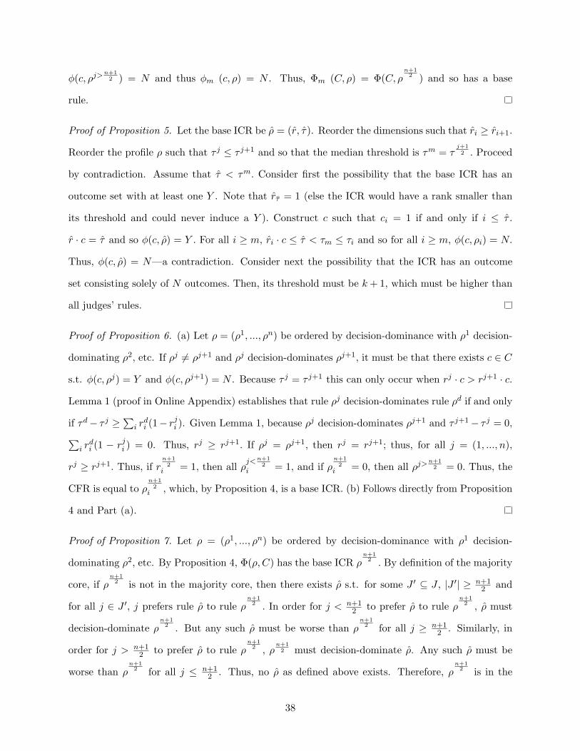
φ(c, ρj>n+1

2 ) = N and thus φm (c, ρ) = N . Thus, Φm (C, ρ) = Φ(C, ρn+1

2 ) and so has a base

rule.

Proof of Proposition 5. Let the base ICR be ρ̂ = (r̂, τ̂). Reorder the dimensions such that r̂i ≥ r̂i+1.

Reorder the profile ρ such that τ j ≤ τ j+1 and so that the median threshold is τm = τj+12 . Proceed

by contradiction. Assume that τ̂ < τm. Consider first the possibility that the base ICR has an

outcome set with at least one Y . Note that r̂τ̄ = 1 (else the ICR would have a rank smaller than

its threshold and could never induce a Y ). Construct c such that ci = 1 if and only if i ≤ τ̂ .

r̂ · c = τ̂ and so φ(c, ρ̂) = Y . For all i ≥ m, r̂i · c ≤ τ̂ < τm ≤ τi and so for all i ≥ m, φ(c, ρi) = N.

Thus, φ(c, ρ̂) = N—a contradiction. Consider next the possibility that the ICR has an outcome

set consisting solely of N outcomes. Then, its threshold must be k+ 1, which must be higher than

all judges’ rules.

Proof of Proposition 6. (a) Let ρ = (ρ1, ..., ρn) be ordered by decision-dominance with ρ1 decision-

dominating ρ2, etc. If ρj 6= ρj+1 and ρj decision-dominates ρj+1, it must be that there exists c ∈ C

s.t. φ(c, ρj) = Y and φ(c, ρj+1) = N . Because τ j = τ j+1 this can only occur when rj · c > rj+1 · c.

Lemma 1 (proof in Online Appendix) establishes that rule ρj decision-dominates rule ρd if and only

if τd− τ j ≥∑

i rdi (1− r

ji ). Given Lemma 1, because ρj decision-dominates ρj+1 and τ j+1− τ j = 0,∑

i rdi (1 − rji ) = 0. Thus, rj ≥ rj+1. If ρj = ρj+1, then rj = rj+1; thus, for all j = (1, ..., n),

rj ≥ rj+1. Thus, if rn+1

2i = 1, then all ρ

j<n+12

i = 1, and if ρn+1

2i = 0, then all ρj>

n+12 = 0. Thus, the

CFR is equal to ρn+1

2i , which, by Proposition 4, is a base ICR. (b) Follows directly from Proposition

4 and Part (a).

Proof of Proposition 7. Let ρ = (ρ1, ..., ρn) be ordered by decision-dominance with ρ1 decision-

dominating ρ2, etc. By Proposition 4, Φ(ρ, C) has the base ICR ρn+1

2 . By definition of the majority

core, if ρn+1

2 is not in the majority core, then there exists ρ̂ s.t. for some J ′ ⊆ J , |J ′| ≥ n+12 and

for all j ∈ J ′, j prefers rule ρ̂ to rule ρn+1

2 . In order for j < n+12 to prefer ρ̂ to rule ρ

n+12 , ρ̂ must

decision-dominate ρn+1

2 . But any such ρ̂ must be worse than ρn+1

2 for all j ≥ n+12 . Similarly, in

order for j > n+12 to prefer ρ̂ to rule ρ

n+12 , ρ

n+12 must decision-dominate ρ̂. Any such ρ̂ must be

worse than ρn+1

2 for all j ≤ n+12 . Thus, no ρ̂ as defined above exists. Therefore, ρ

n+12 is in the

38

majority core.

Proof of Proposition 8. (a) Suppose that a base ICR does not exist. It must, then, be true that

there exists no base legal rule that yields Φm (C, ρ). Let ρ̄(ρ) be the CFR. ρ̄(ρ) always exists and

is a base rule. It follows that the (complex) legal rule ρ̂ such that Φ(C, ρ̂) = Φm (C, ρ) is not

equivalent to ρ̄(ρ), that is, Φ(C, ρ̂) 6= Φ(C, ρ̄(ρ)). Therefore, there must exist at least one case

c1 ∈ C such that φ(c1, ρ̂) 6= φ(c1, ρ̄(ρ)). It follows that ρ must manifest the Generalized Doctrinal

Paradox. (b) Example 5 shows that Part (b) of this Proposition is not vacuous. Suppose that ρj

is the base ICR given Φm (C, ρ) and that Φ(C, ρj) 6= Φ(C, ρ̄(ρ)). It follows that there exists C̃ ⊆ C

such that for all ci ∈ C̃, φ(ci, ρj) 6= φ(ci, ρ̄(ρ)) and for all ck ∈ C\C̃ (the set C\C̃ possibly empty),

φ(ck, ρj) = φ(ck, ρ̄(ρ)). Because ρj is the base ICR, it follows that for all and only ci ∈ C̃, the

(overall judgment) majority decisions differ from the corresponding decisions induced by ρ̄(ρ)—that

is ρ must manifest the Generalized Doctrinal Paradox, and ci ∈ C̃ are all and only cases in C that

give rise to it. (c) The contradiction of this would require the same rule to produce a different set

of case outcomes, which is obviously impossible.

39

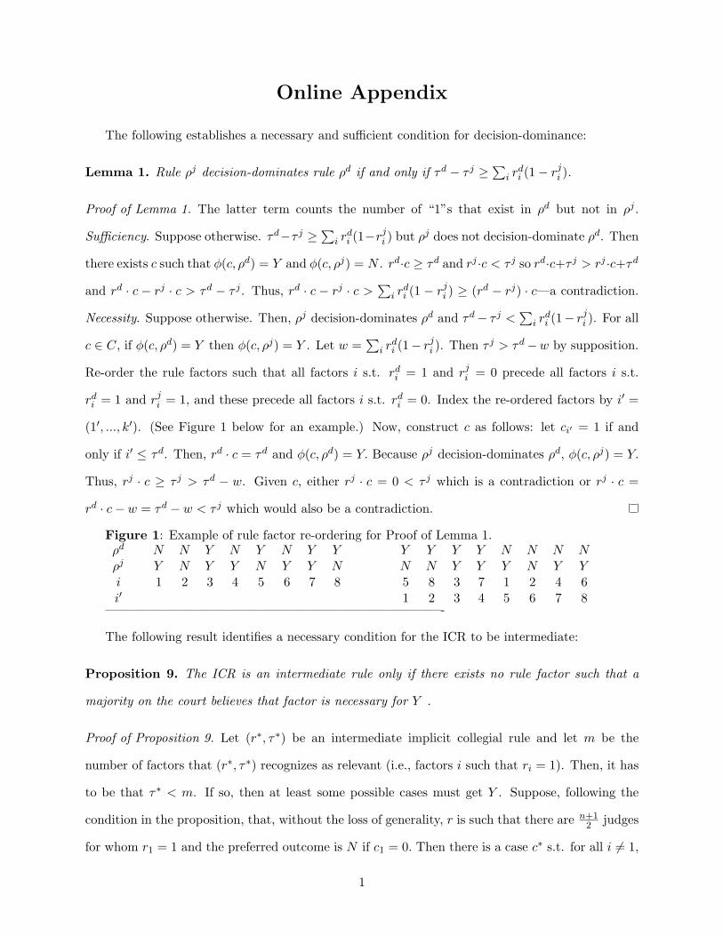
Online Appendix

The following establishes a necessary and sufficient condition for decision-dominance:

Lemma 1. Rule ρj decision-dominates rule ρd if and only if τd − τ j ≥∑

i rdi (1− r

ji ).

Proof of Lemma 1. The latter term counts the number of “1”s that exist in ρd but not in ρj .

Sufficiency. Suppose otherwise. τd−τ j ≥∑

i rdi (1−r

ji ) but ρj does not decision-dominate ρd. Then

there exists c such that φ(c, ρd) = Y and φ(c, ρj) = N . rd·c ≥ τd and rj ·c < τ j so rd·c+τ j > rj ·c+τd

and rd · c − rj · c > τd − τ j . Thus, rd · c − rj · c >∑

i rdi (1 − r

ji ) ≥ (rd − rj) · c—a contradiction.

Necessity. Suppose otherwise. Then, ρj decision-dominates ρd and τd− τ j <∑

i rdi (1− r

ji ). For all

c ∈ C, if φ(c, ρd) = Y then φ(c, ρj) = Y . Let w =∑

i rdi (1− r

ji ). Then τ j > τd−w by supposition.

Re-order the rule factors such that all factors i s.t. rdi = 1 and rji = 0 precede all factors i s.t.

rdi = 1 and rji = 1, and these precede all factors i s.t. rdi = 0. Index the re-ordered factors by i′ =

(1′, ..., k′). (See Figure 1 below for an example.) Now, construct c as follows: let ci′ = 1 if and

only if i′ ≤ τd. Then, rd · c = τd and φ(c, ρd) = Y. Because ρj decision-dominates ρd, φ(c, ρj) = Y.

Thus, rj · c ≥ τ j > τd − w. Given c, either rj · c = 0 < τ j which is a contradiction or rj · c =

rd · c− w = τd − w < τ j which would also be a contradiction.

Figure 1: Example of rule factor re-ordering for Proof of Lemma 1.ρd N N Y N Y N Y Y Y Y Y Y N N N Nρj Y N Y Y N Y Y N N N Y Y Y N Y Yi 1 2 3 4 5 6 7 8 5 8 3 7 1 2 4 6i′ 1 2 3 4 5 6 7 8

——————————————————————————-

The following result identifies a necessary condition for the ICR to be intermediate:

Proposition 9. The ICR is an intermediate rule only if there exists no rule factor such that a

majority on the court believes that factor is necessary for Y .

Proof of Proposition 9. Let (r∗, τ∗) be an intermediate implicit collegial rule and let m be the

number of factors that (r∗, τ∗) recognizes as relevant (i.e., factors i such that ri = 1). Then, it has

to be that τ∗ < m. If so, then at least some possible cases must get Y . Suppose, following the

condition in the proposition, that, without the loss of generality, r is such that there are n+12 judges

for whom r1 = 1 and the preferred outcome is N if c1 = 0. Then there is a case c∗ s.t. for all i 6= 1,

1

c∗i = 1 and c1 = 0 in which the collegial outcome is N. What base implicit collegial rule would be

consistent with such an outcome? First, it has to be that r∗1 = 1, else, by properness, we must have

Y in c∗. But if (r∗, τ∗) is intermediate, then τ∗ < m, in which case, by properness, we should have

reached an outcome Y in c∗. Hence (r∗, τ∗) cannot have been an intermediate rule.

——————————————————————————-

An example in which collegiality increases coherence (We thank an anonymous reviewer

for this example): Consider three judges (J1, J2, and J3) and four factors (C1, C2, C3, and C4).

Suppose that a coherent (libertarian) legal philosophy would require a Y outcome if and only if

C1=1, with the other three factors irrelevant. C2, C3, and C4 therefore represent “incoherent”

individualistic biases. For example, the Y/N decision might be “Is the enforcement of this libel

law unconstitutional,” C1 might be “Does the enforcement of the law in this case suppress political

speech?,” while C2, C3, and C4 are, respectively, “Was the enforcement target someone other than

a communist?”; “Was the enforcement target someone other than a pornographer?”; and “Was

the enforcement target someone other than a white supremacist?” Suppose the three individual

judge rules are such that each requires C1 along with one of the biased factors (C2, C3, and C4

respectively). In this example, the individual preferred rules are “incoherent” in that they all

contain ad hoc exceptions to a general “libertarian” principal that suppression of political speech

is unlawful. But the collective rule is coherent, at least in this sense, because while there is

majority support for the general principle (Y if C1=1), there is not majority support for any of the

particularistic exceptions.

———————————————————————————————————————

2

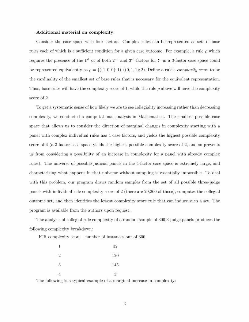
Additional material on complexity:

Consider the case space with four factors. Complex rules can be represented as sets of base

rules each of which is a sufficient condition for a given case outcome. For example, a rule ρ which

requires the presence of the 1st or of both 2nd and 3rd factors for Y in a 3-factor case space could

be represented equivalently as ρ = {((1, 0, 0); 1), ((0, 1, 1); 2). Define a rule’s complexity score to be

the cardinality of the smallest set of base rules that is necessary for the equivalent representation.

Thus, base rules will have the complexity score of 1, while the rule ρ above will have the complexity

score of 2.

To get a systematic sense of how likely we are to see collegiality increasing rather than decreasing

complexity, we conducted a computational analysis in Mathematica. The smallest possible case

space that allows us to consider the direction of marginal changes in complexity starting with a

panel with complex individual rules has 4 case factors, and yields the highest possible complexity

score of 4 (a 3-factor case space yields the highest possible complexity score of 2, and so prevents

us from considering a possibility of an increase in complexity for a panel with already complex

rules). The universe of possible judicial panels in the 4-factor case space is extremely large, and

characterizing what happens in that universe without sampling is essentially impossible. To deal

with this problem, our program draws random samples from the set of all possible three-judge

panels with individual rule complexity score of 2 (there are 29,260 of those), computes the collegial

outcome set, and then identifies the lowest complexity score rule that can induce such a set. The

program is available from the authors upon request.

The analysis of collegial rule complexity of a random sample of 300 3-judge panels produces the

following complexity breakdown:

ICR complexity score number of instances out of 300

1 32

2 120

3 145

4 3The following is a typical example of a marginal increase in complexity:

3

Example 9. Consider a 4-factor case space and the following panel of judges:

ρ1 = {((1, 0, 0, 0); 1), ((0, 1, 1, 1); 3),

ρ2 = {((0, 1, 0, 0); 1), ((1, 0, 1, 0); 2),

ρ1 = {((0, 0, 0, 1); 1), ((0, 1, 1, 0); 2).

Each judge’s rule has a complexity score of 2. A majority of judges will vote Y on the following

list of cases (and will vote N on all others): (1, 1, 1, 1), (0, 1, 1, 1), (1, 1, 1, 0), (1, 0, 1, 1), (1, 1, 0, 0),

(1, 0, 1, 0), (1, 0, 0, 1), (0, 1, 0, 1). This collegial outcome set yields the following complex implicit

collegial rule:

{((1, 1, 1, 0); 2), ((1, 0, 0, 1); 2), ((0, 1, 0, 1); 2)},

which has a complexity score of 3.

4