Lee, Zhi Hou (2015) Improved multiple input multiple...
174
Lee, Zhi Hou (2015) Improved multiple input multiple output blind equalization algorithms for medical implant communication. PhD thesis, University of Nottingham. Access from the University of Nottingham repository: http://eprints.nottingham.ac.uk/28726/1/PhD_Thesis_LeeZhiHou_2015.pdf Copyright and reuse: The Nottingham ePrints service makes this work by researchers of the University of Nottingham available open access under the following conditions. This article is made available under the University of Nottingham End User licence and may be reused according to the conditions of the licence. For more details see: http://eprints.nottingham.ac.uk/end_user_agreement.pdf For more information, please contact [email protected]
Transcript of Lee, Zhi Hou (2015) Improved multiple input multiple...

Lee, Zhi Hou (2015) Improved multiple input multiple output blind equalization algorithms for medical implant communication. PhD thesis, University of Nottingham.
Access from the University of Nottingham repository: http://eprints.nottingham.ac.uk/28726/1/PhD_Thesis_LeeZhiHou_2015.pdf
Copyright and reuse:
The Nottingham ePrints service makes this work by researchers of the University of Nottingham available open access under the following conditions.
This article is made available under the University of Nottingham End User licence and may be reused according to the conditions of the licence. For more details see: http://eprints.nottingham.ac.uk/end_user_agreement.pdf
For more information, please contact [email protected]
IMPROVED MULTIPLE INPUT
MULTIPLE OUTPUT BLIND
EQUALIZATION ALGORITHMS
FOR MEDICAL IMPLANT
COMMUNICATION
LEE ZHI HOU, MEng.
Thesis submitted to the University of Nottingham
for the degree of Doctor of Philosophy
APRIL 2015
Abstract
Medical implant sensor that is used to monitor the human physiology signals is helpful to im-
prove the quality of life and prevent severe result from the chronic diseases. In order to achieve
this, the wireless implant communication link that delivers the monitored signal to a multiple
antennas external device is an essential portion. However, the existing conventional narrow band
Medical Implant Communications System (MICS) has low data rate because of the bandlimited
channel is allocated. To improve the data rate in the radio frequency communication, ultra-wide
band technology has been proposed. However, the ultra-wide band technology is relatively new
and requires living human to be the test subject in order to validate the technology performance.
In this condition, the test on the new technology can rise ethical challenge. As a solution, we
improve the data rate in the conventional narrow band MICS. The improvement of data rate on
the narrow band implies the information bandwidth is larger than the allocated channel band-
width, and therefore the high frequency components of the information can loss. In this case, the
signal suffers the intersymbol-interference (ISI). Instead of that, the multiple antennas external
device can receive the signal from other transmitting implant sensor which has the same operating
frequency. As a result, the signal is further hampered by co-channel interference (CCI). To recover
the signal from the ISI and CCI, multiple-input multiple output (MIMO) blind equalization that
has source separation ability can be exploited. Cross-Correlation Constant Modulus Algorithm
(CC-CMA) is the conventional MIMO blind equalization algorithm that can suppress ISI and CCI
i
and able to perform source separation. However, CC-CMA has only been analyzed and simulated
in the modulation of Phase Shift Keying (PSK). The performance of CC-CMA in multi-modulus
modulation scheme such as 4-Pulse-amplitude modulation (PAM) and 16-Quadrature amplitude
modulation (QAM), which has higher data rate than PSK, has not been analyzed. Therefore, our
work is to analysis and optimize CC-CMA on the multi-modulus modulation scheme. From our
analysis, we found that the cost function of CC-CMA is biased cost function. Instead of that,
from our simulation, CC-CMA introduces an unexpected shrinking effect whereby the amplitudes
of the equalizer outputs have been reduced, especially in multi-modulus modulation scheme. This
shrinking effect is not severe in PSK because the decision of a PSK symbol is based on phase, but
not amplitude. Unfortunately, this is severe in multi-modulus modulation scheme. To overcome
this shrinking effect in multi-modulus modulation scheme, we propose Cross-Independent Constant
Modulus Algorithm (CI-CMA). Based on the convergence analysis, we identify the new optimum
dispersion value and mixing parameter in CI-CMA. From the simulation results, we confirm that
CI-CMA is able to perform equalization and source separation in the multi-modulus modulation
scheme. In order to improve the steady state performance of CI-CMA, we perform the steady
state mean square error (MSE) analysis of CI-CMA using the energy preservation theorem that
was developed by Mai and Sayed in 2001, and our result is more accurate than the previous work.
From our analysis, only the reduction in adaptation step size can reduce the steady state MSE,
but it is well known that the MSE is indeed a tradeoff with the speed of convergence. Therefore
without sacrificing convergence speed, our last effort is to propose hybrid algorithms. The hybrid
algorithms are done by combining a new adaptive constant modulus algorithm (ACMA), a decision
directed algorithm and a cross-correlation function. From the simulation results, we found that
the hybrid algorithms can show low steady state error and thereby improve the reliability of the
communication link. The main achievement of this thesis is the discovery of new dispersion value
through the convergence analysis.
ii

Acknowledgements
I would like to express my gratitude to my supervisor, Dr Lim Wee Gin for his guidance and
encouragement. I have learned so much from him. Without his patience and understanding, this
thesis would never be completed.
I am also grateful to my thesis examiners, Dr Amin Malek Mohammadi and Ir. Dr. Tiong Sieh
Kiong. I also would like to thank to my 1st and 2nd year internal accessor, Dr Khalid Al Murrani
for his useful feedback.
I am greatly indebted to the Department of Electrical and Electronic Engineering, the Univer-
sity of Nottingham Malaysia Campus for awarding me a PhD scholarship and a golden opportunity
to become a research assistant.
Finally, I would like to thank my family and friends for their support and encouragement.
iii
Contents
Abstract i
Acknowledgements iii
List of Abbreviations viii
List of Figures xi
List of Tables xiv
1 Introduction 1
1.1 Background . . . . . . . . . . . . . . . . . . . . . . . . . . . . . . . . . . . . . . . . 2
1.2 Practical Challenges . . . . . . . . . . . . . . . . . . . . . . . . . . . . . . . . . . . 4
1.3 Practical Objectives and Proposed Solutions . . . . . . . . . . . . . . . . . . . . . . 6
1.4 Research Background . . . . . . . . . . . . . . . . . . . . . . . . . . . . . . . . . . 7
1.5 Research Limitations and Objectives . . . . . . . . . . . . . . . . . . . . . . . . . . 10
1.5.1 Robust to 4-PAM and 16-QAM . . . . . . . . . . . . . . . . . . . . . . . . . 10
1.5.2 Superior Steady State Performance is required . . . . . . . . . . . . . . . . 10
1.6 Contributions . . . . . . . . . . . . . . . . . . . . . . . . . . . . . . . . . . . . . . . 11
1.7 Structure of the thesis . . . . . . . . . . . . . . . . . . . . . . . . . . . . . . . . . . 13
2 Literature Review 14
2.1 Introduction . . . . . . . . . . . . . . . . . . . . . . . . . . . . . . . . . . . . . . . . 14
2.2 Chronic diseases and wireless medical sensor . . . . . . . . . . . . . . . . . . . . . . 15
iv
2.3 Wearable sensor . . . . . . . . . . . . . . . . . . . . . . . . . . . . . . . . . . . . . . 15
2.4 Implant sensor . . . . . . . . . . . . . . . . . . . . . . . . . . . . . . . . . . . . . . 17
2.5 Applications of implant sensor . . . . . . . . . . . . . . . . . . . . . . . . . . . . . 17
2.5.1 Blood glucose level monitoring . . . . . . . . . . . . . . . . . . . . . . . . . 17
2.5.2 Cardiovascular system monitoring . . . . . . . . . . . . . . . . . . . . . . . 18
2.5.3 Cancer detector . . . . . . . . . . . . . . . . . . . . . . . . . . . . . . . . . . 18
2.5.4 Capsule endoscopy . . . . . . . . . . . . . . . . . . . . . . . . . . . . . . . . 19
2.6 Current and Potential Implant Communications . . . . . . . . . . . . . . . . . . . . 20
2.6.1 MICS standard . . . . . . . . . . . . . . . . . . . . . . . . . . . . . . . . . . 20
2.6.2 UWB communication . . . . . . . . . . . . . . . . . . . . . . . . . . . . . . 21
2.6.3 Human Body Communication . . . . . . . . . . . . . . . . . . . . . . . . . . 23
2.6.4 Summary . . . . . . . . . . . . . . . . . . . . . . . . . . . . . . . . . . . . . 23
2.7 Interferences and MIMO channel equalization . . . . . . . . . . . . . . . . . . . . . 24
2.8 System model and Assumptions . . . . . . . . . . . . . . . . . . . . . . . . . . . . . 26
2.9 Definition of a Good MIMO Blind Equalizer . . . . . . . . . . . . . . . . . . . . . . 30
2.10 Time Domain Identification of Good MIMO Equalizer (with examples) . . . . . . . 36
2.11 The way of adaptation in MIMO equalizer . . . . . . . . . . . . . . . . . . . . . . . 38
2.12 Performance Measurements . . . . . . . . . . . . . . . . . . . . . . . . . . . . . . . 39
2.13 Review on SISO Blind Equalization Algorithms . . . . . . . . . . . . . . . . . . . . 40
2.14 Review on SISO Hybrid Algorithms . . . . . . . . . . . . . . . . . . . . . . . . . . 44
2.14.1 Stop-And-Go Algorithm Decision Directed Algorithm (SAG) . . . . . . . . 45
2.14.2 Benveniste-Goursat Algorithm (BG) . . . . . . . . . . . . . . . . . . . . . . 46
2.14.3 Reliability Based Algorithm (RBA) . . . . . . . . . . . . . . . . . . . . . . 46
2.15 MIMO Blind equalization and source separation algorithms . . . . . . . . . . . . . 47
2.15.1 Source separation algorithm . . . . . . . . . . . . . . . . . . . . . . . . . . . 48
2.15.2 Pure equalization algorithm . . . . . . . . . . . . . . . . . . . . . . . . . . . 50
v
2.15.3 Single task algorithm . . . . . . . . . . . . . . . . . . . . . . . . . . . . . . . 50
2.15.4 Two tasks algorithm . . . . . . . . . . . . . . . . . . . . . . . . . . . . . . . 50
3 Cross-Independent Constant Modulus Algorithm 56
3.1 Introduction . . . . . . . . . . . . . . . . . . . . . . . . . . . . . . . . . . . . . . . . 56
3.2 Background . . . . . . . . . . . . . . . . . . . . . . . . . . . . . . . . . . . . . . . . 58
3.2.1 System model and assumptions . . . . . . . . . . . . . . . . . . . . . . . . . 58
3.2.2 Classical mixed cost approach . . . . . . . . . . . . . . . . . . . . . . . . . . 60
3.2.3 Motivation: shrinking of the equalizer output . . . . . . . . . . . . . . . . . 61
3.3 New Cross Independent Constant Modulus Algorithm (CI-CMA) . . . . . . . . . . 64
3.3.1 A new BSS cost: the cross independent function . . . . . . . . . . . . . . . 64
3.3.2 Preliminary assumptions and useful notations . . . . . . . . . . . . . . . . . 65
3.3.3 Extrema analysis . . . . . . . . . . . . . . . . . . . . . . . . . . . . . . . . . 66
3.3.4 Design of new dispersion constant, Rj . . . . . . . . . . . . . . . . . . . . . 68
3.3.5 Stability analysis . . . . . . . . . . . . . . . . . . . . . . . . . . . . . . . . . 70
3.3.6 Design of mixing parameter, k0 . . . . . . . . . . . . . . . . . . . . . . . . . 72
3.4 Extension to complex modulations . . . . . . . . . . . . . . . . . . . . . . . . . . . 74
3.5 Simulations . . . . . . . . . . . . . . . . . . . . . . . . . . . . . . . . . . . . . . . . 76
3.5.1 Simulation Setup . . . . . . . . . . . . . . . . . . . . . . . . . . . . . . . . . 76
3.5.2 Simulation Parameters . . . . . . . . . . . . . . . . . . . . . . . . . . . . . . 78
3.5.3 Performance measurements . . . . . . . . . . . . . . . . . . . . . . . . . . . 80
3.5.4 Simulation results for 2-PAM signal . . . . . . . . . . . . . . . . . . . . . . 81
3.5.5 Simulation results for 4-PAM signal . . . . . . . . . . . . . . . . . . . . . . 84
3.5.6 Simulation results for 4-QAM signal . . . . . . . . . . . . . . . . . . . . . . 87
3.5.7 Simulation results for 16-QAM signal . . . . . . . . . . . . . . . . . . . . . 90
3.5.8 Summary . . . . . . . . . . . . . . . . . . . . . . . . . . . . . . . . . . . . . 92
vi
4 Steady State MSE Analysis of the CI-CMA 93
4.1 Introduction . . . . . . . . . . . . . . . . . . . . . . . . . . . . . . . . . . . . . . . . 93
4.2 System model and assumptions . . . . . . . . . . . . . . . . . . . . . . . . . . . . . 94
4.3 The CI-CMA . . . . . . . . . . . . . . . . . . . . . . . . . . . . . . . . . . . . . . . 96
4.4 Steady state MSE analysis of CI-CMA . . . . . . . . . . . . . . . . . . . . . . . . . 97
4.4.1 Recap on energy-preserving theorem and assumptions . . . . . . . . . . . . 97
4.4.2 Analysis on L.H.S. of Eq. 4.18 . . . . . . . . . . . . . . . . . . . . . . . . . 99
4.4.3 Analysis on R.H.S. of Eq. 4.18 . . . . . . . . . . . . . . . . . . . . . . . . . 103
4.4.4 Expression of the Steady State MSE . . . . . . . . . . . . . . . . . . . . . . 104
4.5 Simulations . . . . . . . . . . . . . . . . . . . . . . . . . . . . . . . . . . . . . . . . 105
4.5.1 Simulation Setup . . . . . . . . . . . . . . . . . . . . . . . . . . . . . . . . . 105
4.5.2 Discussion . . . . . . . . . . . . . . . . . . . . . . . . . . . . . . . . . . . . . 109
5 Hybrid Algorithms for MIMO Equalization 111
5.1 Introduction . . . . . . . . . . . . . . . . . . . . . . . . . . . . . . . . . . . . . . . . 111
5.2 System model and assumptions . . . . . . . . . . . . . . . . . . . . . . . . . . . . . 112
5.3 Blind Adaptive Hybrid Algorithms For MIMO Systems . . . . . . . . . . . . . . . 114
5.3.1 General cost function . . . . . . . . . . . . . . . . . . . . . . . . . . . . . . 114
5.3.2 Acquisition, Source Separation and Tracking algorithms . . . . . . . . . . . 115
5.3.3 MIMO Hybrid algorithms . . . . . . . . . . . . . . . . . . . . . . . . . . . . 117
5.3.4 CI-CMA . . . . . . . . . . . . . . . . . . . . . . . . . . . . . . . . . . . . . . 119
5.3.5 Previous works . . . . . . . . . . . . . . . . . . . . . . . . . . . . . . . . . . 119
5.4 Simulations . . . . . . . . . . . . . . . . . . . . . . . . . . . . . . . . . . . . . . . . 120
5.4.1 Simulation Setup . . . . . . . . . . . . . . . . . . . . . . . . . . . . . . . . . 120
5.4.2 Performance measurements . . . . . . . . . . . . . . . . . . . . . . . . . . . 122
5.4.3 Simulation results . . . . . . . . . . . . . . . . . . . . . . . . . . . . . . . . 123
5.4.4 Discussion . . . . . . . . . . . . . . . . . . . . . . . . . . . . . . . . . . . . . 130
vii
6 Conclusions and Future works 134
6.1 Conclusions . . . . . . . . . . . . . . . . . . . . . . . . . . . . . . . . . . . . . . . . 134
6.2 Future Works . . . . . . . . . . . . . . . . . . . . . . . . . . . . . . . . . . . . . . . 136
A Proof of Equations 137
A.1 Proof of independence of the CI cost (3.7) and (3.19) . . . . . . . . . . . . . . . . . 137
A.2 Stationary Point Analysis: Derivation of (3.31) . . . . . . . . . . . . . . . . . . . . 139
References 137
List of Publications 157
viii

List of Abbreviations ACMA Adaptive Constant Modulus Algorithm ADC Analog to Digital Convertor ASK Amplitude Shift Keying AWGN Additive White Gaussian Noises BG Benveniste Goursat Algorithm BPSK Binary Phase Shift Keying BSS Blind Source Separation BSS-CMA Blind Source Separation Constant Modulus Algorithm BSS-MMA Blind Source Separation Multi Modulus Algorithm CC Cross Correlation CC-CMA Cross-Correlation Constant Modulus Algorithm CCI Co-Channel Interference CC-SCMA Cross-Correlation Simplified Constant Modulus Algorithm CDMA Code Division Multiplexing Access CI Cross Independent CI-CMA Crosee-Independent Constant Modulus Algorithm CMA Constant Modulus Algorithm dB Decibel DD Decision Directed DNA Deoxyribonucleic Acid DPSK Differential Phase Shift Keying FA Factor Analysis FIR Finite Impulse Responses FSK Frequency Shift Keying HBC Human Body Communication HF High Frequency i.i.d. Identical and Independent Distributed ICA Independent Component Analysis
ix
IEEE Institute of Electrical and Electronics Engineers IF Intermediate Frequency IR Impulse Radio ISI Inter-Symbol Interference IT Residual Interference Kur Kurtosis L.H.S. Left Hand Side LAN Local Area Network LMS Least Mean Square MAP Maximum A Posteriori MATLAB Matrix Laboratory MB-OFDM Multi Band Orthogonal Frequency-Division Multiple MCIBG Modified Cross Independent Benveniste-Goursat Algorithm MCIRBA Modified Cross Independent Reliability Based Algorithm MCISAG Modified Cross Independent Stop and Go Algorithm MICS Medical Implant Communications System MIMO Multiple Inputs Multiple Outputs MIMO-CMA Multiple Inputs Multiple Outputs Constant Modulus Algorithm MSE Mean Square Error NB Narrow Band OFDM Orthogonal Frequency-Division Multiple O-MMA Orthogonal Multi Modulus Algorithm OOK On/Off Keying PAM Pulse Amplitude Modulation PAPR Peak-to-Average Power Ratio PCA Principle Component Analysis PSK Phase Shift Keying QAM Quadrature Amplitude Modulation QPSK Quadrature Phase Shift Keying R.H.S. Right Hand Side RBA Reliability Based Algorithm RF Radio Frequency SAG Stop-And-Go Algorithm Decision Directed Algorithm SGA Stochastic Gradient descent Algorithm Sim Simulation SISO Single-Input Single-Output Th Theoretical UHF Ultra High Frequency UWB Ultra Wide Band VHF Very High Frequency WLAN Wireless Local Area Network
x
List of Figures
2.1 Baseband equivalent system for Mt = 2 and Mr = 3. . . . . . . . . . . . . . . . . . 26
2.2 MIMO system . . . . . . . . . . . . . . . . . . . . . . . . . . . . . . . . . . . . . . . 33
3.1 Baseband equivalent system for Mt = 2 and Mr = 3. . . . . . . . . . . . . . . . . . 59
3.2 (a) Residual interference (IT) of equalizer 1. (b) IT of equalizer 2. (c) First half: the
averaged global impulse responses taken from time k = 199, 000 to time k = 200, 000.
Source separation is not successful. (d) Second half: the averaged global impulse responses
taken from time k = 399, 000 to time k = 400, 000. Source is not changed in equalizer 2. . 81
3.3 Output signals of equalizers 1 and 2. . . . . . . . . . . . . . . . . . . . . . . . . . . . 81
3.4 (a) Residual interference (IT) of equalizer 1. (b) IT of equalizer 2. (c) First half: the
averaged global impulse responses taken from time k = 599, 000 to time k = 600, 000. The
apparent success in source separation is not yet conclusive. (d) Second half: the averaged
global impulse responses taken from time k = 1, 199, 000 to time k = 1, 200, 000. Source
separation is proven successful. . . . . . . . . . . . . . . . . . . . . . . . . . . . . . . 84
3.5 Output signals of equalizers 1 and 2. . . . . . . . . . . . . . . . . . . . . . . . . . . . 84
3.6 (a) Residual interference (IT) of equalizer 1. (b) IT of equalizer 2. (c) First half: the
averaged global impulse responses taken from k = 599, 000 to k = 600, 000. Source separa-
tion is not successful. (d) Second half: the averaged global impulse responses taken from
k = 1, 199, 000 to k = 1, 200, 000. Source is not changed in equalizer 2. . . . . . . . . . . 87
xi
3.7 Output signals of equalizers 1 and 2 at steady state. . . . . . . . . . . . . . . . . . . . 87
3.8 (a) Residual interference (IT) of equalizer 1. (b) IT of equalizer 2. (c) First half: the
averaged global impulse responses taken from k = 599, 000 to k = 600, 000. The apparent
success in source separation is not yet conclusive. (d) Second half: the averaged global
impulse responses taken from k = 1, 199, 000 to k = 1, 200, 000. Source separation is proven
successful. . . . . . . . . . . . . . . . . . . . . . . . . . . . . . . . . . . . . . . . . . 90
3.9 Output signals of equalizers 1 and 2 at steady state. . . . . . . . . . . . . . . . . . . . 90
4.1 Baseband equivalent system for Mt = 2 and Mr = 3. . . . . . . . . . . . . . . . . . 95
4.2 Simulation and theoretical curves for the steady state MSE as a function of mixing
parameter, kj with µj = 1× 10⁻⁷ from a 16-QAM constellation for equalizer 2, j = 2.108
4.3 Simulation and theoretical curves for the steady state MSE as a function of step size,
µj with mixing parameter, kj = 1.41 from a 16-QAM constellation for equalizer 2,
j = 2. . . . . . . . . . . . . . . . . . . . . . . . . . . . . . . . . . . . . . . . . . . . 109
5.1 Baseband equivalent system for Mt = 2 and Mr = 3. . . . . . . . . . . . . . . . . . 113
5.2 Performance comparison of different algorithms for equalizer 1 and 2. Hybrid algo-
rithms provide superior performance than others. . . . . . . . . . . . . . . . . . . . 123
5.3 Equalizer outputs of CC-CMA at the steady state. The symbols closely match with
the 16-QAM constellation set for equalizer 1 but the symbols of equalizer 2 have
been shrunk. . . . . . . . . . . . . . . . . . . . . . . . . . . . . . . . . . . . . . . . 124
5.4 The averaged global impulse responses of CC-CMA taken in the steady state. Source
separation is successful but a down-scaling of 0.2 has been introduced to the equalizer
2. . . . . . . . . . . . . . . . . . . . . . . . . . . . . . . . . . . . . . . . . . . . . . . 124
5.5 Equalizer outputs of MIMO-CMA at the steady state. The symbols closely match
with the 16-QAM constellation set for equalizer 1 and 2 . . . . . . . . . . . . . . . 125
xii
5.6 The averaged global impulse responses of MIMO-CMA taken in the steady state.
Source separation is not successful. . . . . . . . . . . . . . . . . . . . . . . . . . . . 125
5.7 Equalizer outputs of CI-CMA at the steady state. . . . . . . . . . . . . . . . . . . 126
5.8 The averaged global impulse responses of CI-CMA taken in the steady state. Source
separation is successful. . . . . . . . . . . . . . . . . . . . . . . . . . . . . . . . . . 126
5.9 Equalizer outputs of MCIBG at the steady state. . . . . . . . . . . . . . . . . . . . 127
5.10 The averaged global impulse responses of MCIBG taken in the steady state. Source
separation is successful. . . . . . . . . . . . . . . . . . . . . . . . . . . . . . . . . . 127
5.11 Equalizer outputs of MCIRBA at the steady state. . . . . . . . . . . . . . . . . . . 128
5.12 The averaged global impulse responses of MCIRBA taken in the steady state. Source
separation is successful. . . . . . . . . . . . . . . . . . . . . . . . . . . . . . . . . . 128
5.13 Equalizer outputs of MCISAG at the steady state. . . . . . . . . . . . . . . . . . . 129
5.14 The averaged global impulse responses of MCISAG taken in the steady state. Source
separation is successful. . . . . . . . . . . . . . . . . . . . . . . . . . . . . . . . . . 129
xiii
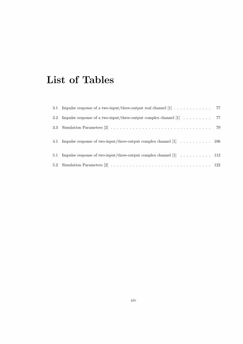
List of Tables
3.1 Impulse response of a two-input/three-output real channel [1] . . . . . . . . . . . . 77
3.2 Impulse response of a two-input/three-output complex channel [1] . . . . . . . . . 77
3.3 Simulation Parameters [2] . . . . . . . . . . . . . . . . . . . . . . . . . . . . . . . . 79
4.1 Impulse response of two-input/three-output complex channel [1] . . . . . . . . . . 106
5.1 Impulse response of two-input/three-output complex channel [1] . . . . . . . . . . 112
5.2 Simulation Parameters [2] . . . . . . . . . . . . . . . . . . . . . . . . . . . . . . . . 122
xiv
Chapter 1
Introduction
Chronic diseases, also known as non-communicable diseases, are long-lasting illnesses that may
lead to death and disability. These diseases are frequently preventable or controllable through
early detection, medical treatment and proper life style. Examples of chronic diseases are heart
disease, stroke, diabetes, cancer and etc. Unfortunately, World Health Organization has reported
that chronic diseases caused 60 percent and 68 percent of all deaths in 2002 and 2012, respectively
[3]. This indicates that 8 percent increment in 10 years and the percentage of death caused by
chronic diseases probably increases to 76 percent in 2022. Too late in chronic diseases detection is
the common reason that causes the death. Therefore, in order to reduce the percentage of death
caused by chronic diseases and improve the quality of life, wireless medical sensor can be exploited
to monitor the patient and take necessary action once abnormal condition is detected. More
precisely, the wireless medical sensor can be used to collect various real time physiological signals
such as heart rhythm, blood glucose level, body temperature, blood pressure and etc, without
geographical limitation. Through telecommunication network, doctor can access the physiological
signals to determine any possible harmful symptom of patient. If harmful symptom is detected by
doctor, the patient can be informed to be admitted to hospital for further tests or treatment to
avoid any dreadful event.
1
In general, the wireless medical sensor can be divided into wearable sensor and implant sensor,
which are located on-body and in-body, respectively. Wireless wearable medical sensor, is placed
on the body or patient’s skin in non-invasive way and it is removable. The applications of this
type sensor include blood pressure measurement, body temperature monitoring, heart rhythm
monitoring [4], asthma monitoring [5] and etc. Instead of that, the implant sensor is an electronic
sensor that is placed inside human body via surgery or swallowing. The applications of the implant
sensor include blood glucose level monitoring [6], cardiovascular system monitoring [7], cancer
detector, capsule endoscopy [8] and etc. Wireless communication is the essential element of the
above sensors. Among the wearable and implant sensors, the wireless communication link of the
implant sensor is more challenging than the wearable sensor because the implant sensor is located
inside the human body. Therefore, we will focus on the improvement of the wireless communication
link for the implant sensor.
1.1 Background
The wireless implant communication link, which connects an implant sensor to a multi-antennas
external hand held device, is important in order to ensure the monitored data can be received by
doctor in different geographic area. Due to the limited power in the implant sensor, the implant
sensor is not able to directly send the monitored data to the cellular network or local area network
(LAN). Therefore, the external device, which is required to be placed within 2 meter distance from
the implant sensor, is functioned as a gateway because the external device receives the monitored
data from the implant sensor and then re-transmits the data to the cellular or LAN. In general, the
wireless implant communication is a two way communications link. Therefore, it can be divided
into uplink and downlink, which are the communication link from implant to the external device
and from the external device to implant, respectively. As a monitoring device, uplink is expected
to have high data traffic than downlink because the implant sensor frequently sends the monitored
signal to the external device from time to time. In contrary, downlink is expected to have low data
2
traffic because it is used to configure or reprogram the implant. Therefore, we will put our focus
on the improvement of the uplink implant communication.
In the literature, the implant communication can be accomplished through Medical Implant
Communications Systems (MICS) standard, Ultra-wideband (UWB) Communication and Human
Body Communication. The MICS is a narrowband radio frequency (RF) communication that has
been used in cardiac pacemaker and defibrillator to help heart disease patient since 1999 [9, 10, 11].
However, due to the limited channel bandwidth of 300 kHz, MICS has relatively low data rate. To
overcome the data rate limitation, UWB which has the channel bandwidth of 500 MHz has been
proposed. Instead of that, UWB is relatively immune to frequency selective channel fading and
noise [8]. In spite of that, the application of UWB for implant sensor communication has encoun-
tered difficulty. Currently, the performance of UWB only has been tested on the simulations and
models [11, 8]. The actual result on living human is still unknown. In order to conduct this test,
living human is required to be the test subject. Therefore, this is unethical and probably illegal.
As a result, the results of simulations and models of UWB are hardly to be validate. Instead of
that, human body communication is a relatively new type of non-RF communication where human
body is used as the transmission medium. This type of communication provides high security and
high fidelity because the transmission medium is not shared by others. However, this type com-
munication is unfriendly-user in setup and has a very short transmission range where it is limited
to about 100 centimeter distance. Furthermore, the application of human body communication for
the implant communication may rise ethical challenge because living human is required to be the
test subject.
Due to the reason the application of UWB and human body communication for the implant
communication may encounter the ethical challenge, we put our focus on the data rate improvement
on the narrowband MICS.
3
1.2 Practical Challenges
Currently, the operating frequency range of implant communication has been defined from 402 to
405 MHz, which is also known as Medical Implant Communication Service band with the maximum
channel bandwidth of 300 kHz since 1999, even 13 years earlier than the first publication of IEEE
Body Area Network 802.15.6 [9, 10, 11]. The MICS, which is currently belonged to IEEE Body
Area Network 802.15.6, also defines to the uplink and downlink communications. Therefore, the
application of implant communication in MICS is legally defined by the document. In order to
improve the data rate, the uplink communication of the implant communication can encounter
some unique challenges and the challenges are described as following.
i Limited power resource of implant
The implant device requires a safe and reliable power source. In this case, battery can be
a good choice since battery has been used in other in-body equipment such as pacemaker
for many years and no severe issue has been reported. However, due to the reason that
the battery together with implant is located inside human body, the battery is hardly to
be recharged or replaced. Therefore, the battery has limited life time and thus it can be
considered as expensive resource.
ii Limited computation power and memory of implant
Memory and computation operation consume power and cost. Therefore, in order to save
power resource and memory cost, the computation operation should be designed as simple as
possible and the memory size should be small enough to achieve the basic tasks. Therefore,
in this computation and memory limitation condition, complicated digital signal processing
is not encouraged to be performed on the implant.
iii Intersymbol interference (ISI) due to bandlimited channel
Currently, the maximum channel bandwidth of 300 kHz is allocated for implant communi-
cation and thus, the bandwidth of the information signal is traditionally restricted below
4
300 kHz to avoid any undesired distortion. However, the restriction on the information
bandwidth also limits the data rate. In order to increase the data rate, we suggest that
the information bandwidth to be increased more than the allocated channel bandwidth. In
this case, to avoid the transmit signal does not exceed the allocated channel bandwidth,
the information signal is passed though a bandlimited filter before the signal is transmitted.
Obviously, high frequency components of the information signal are attenuated because the
bandlimited filter has lower bandwidth compared to the bandwidth of the information signal.
In this situation, due to the high frequency components of the information signal are lost,
the receiving external device receives the information signal that is corrupted by intersymbol
interference. The ISI can increase the error rate and cause the whole communication link
becomes unreliable. Therefore, in order to achieve higher data rate and reduce the error rate
in this new approach, the receiving external device is expected to equip with signal processing
method that can cope the ISI.
iv Co-channel Interference (CCI)
In a special scenario such as two patients with the same operating frequency implant devices
are standing side by side, the receiving node can receive a distorted signal which is the
combined signal from the desired and undesired implant devices. This type signal distortion is
called co-channel interference because two or more transmitting implant devices are operating
in the same channel. CCI can strongly reduce the receiver performance. To overcome this
problem, the receiving external device should have a signal processing method that can
suppress CCI and perform source separation.
v Expensive communication link
In order to effectively setup the implant, the costs that include devices cost, deployment
cost, surgery cost, medical cost and monitoring cost are expected to be paid. Instead of
that, the limited battery life time has constraint the duration of the communication link to
a finite time. Therefore, from the perspective of the above costs and power resource, the
5

implant communication link is expensive and thus the method that can produces high data
throughput is required.
1.3 Practical Objectives and Proposed Solutions
Based on the above challenges, we can see that a new solution is demanded and the solution should
able to achieve the following objectives.
• The solution should have light and moderate signal processing on the transmitting implant
and the receiving external device, respectively.
• The solution should have the ability to suppress ISI and CCI simultaneously, and also able
to perform source separation.
• The solution is able to improve data throughput.
In order to achieve the objectives, multiple inputs multiple outputs (MIMO) blind equalizer
with source separation ability, is called MIMO blind equalizer, is proposed as the solution on
the receiver side. Instead of that, pulse-amplitude modulation (PAM) and quadrature amplitude
modulation (QAM) are suggested to be the modulation scheme. The reasons of the proposed
solutions are justified as below.
• MIMO blind equalizer does not require the transmitting implant to perform any
complicated operation.
In order to established communication link, some common wireless technologies such as
Orthogonal Frequency-Division Multiple (OFDM) and Code Division Multiplexing Access
(CDMA), require the transmitter to perform Inverse Fast Fourier Transform operation and
code spreading operation, respectively. Therefore, these operations can burden the transmit-
ting implant. Instead of that, OFDM and CDMA are the wide band technologies. Thus,
the performance of the technologies can degrade if they are applied in the narrow band.
6
Therefore, MIMO blind equalizer is suggested to be applied at the receiving external device
because it does not require the above special operations to be performed on the transmitting
implant. Due to the receiving external device is located outside human body, the battery
replacement or recharge is relatively easy, and thus this allows MIMO blind equalizer to be
applied.
• PAM and QAM modulation schemes can improve the data throughput.
MICS communication has relatively low data throughput because of limited channel band-
width (i.e. up to 300 kHz) and bandwidth inefficiency. The limited channel bandwidth issue
has been explained. Now, we put focus on the bandwidth inefficiency issue. In the literature
of MICS, the relatively simple communication modulation schemes such as on/off keying
(OOK), amplitude shift keying (ASK) [12, 13], frequency shift keying (FSK) [14, 15, 16] and
differential phase shift keying (DPSK) [10] can be found. Compared to multi-modulus PAM
and QAM, the above modulations schemes are relatively bandwidth inefficiency and thereby
can the data throughput is low.
1.4 Research Background
Multiple-input multiple-output (MIMO) technology such as spatial division multiple access (SDMA)
has attracted strong interest in telecommunications field, because of the higher data throughput
compared to single-input single-output (SISO) technology [17, 18, 19]. However, the signal recov-
ery in the MIMO receiver is more difficult compared to the SISO receiver because two primary
obstacles need to be overcome in order to retrieve the all the input signals. Firstly, the signals may
suffer from ISI due to the bandlimited channel. The resulting channel is thus commonly known as
a frequency selective channel where signals of different frequencies will suffer different levels of at-
tenuation. Secondly, due to cochannel system sources, the received signals are overlapped versions
of multiple source signals, i.e., a phenomenon called CCI. To overcome ISI and CCI simultaneously,
7
MIMO equalization which equips with open eye and source separation abilities is used.
Generally, there are two type equalization approaches such as trained equalization and blind
equalization. Trained equalization requires the transmitter periodically sends training sequences to
the receiver in order to open the channel eye. Least Mean Square (LMS) is an example of trained
equalization algorithm [20]. Normally, trained equalization can rapidly suppress interferences.
However, the periodical transmission of the training sequence will reduce the data throughput, and
therefore blind equalization is developed. The blind equalizer exploits the statistical information
of transmitted signals to recover signal instead of training signals. Thus, blind equalization is a
good candidate when the communication link is expensive. In practice, blind equalizer depends on
its algorithm to compute the optimum coefficient. Therefore, blind equalization algorithm is the
key to determine the performance of a blind equalizer.
Many SISO blind equalization algorithms have been developed in the literature. Some blind
equalization algorithms that are supported by theoretical analysis are Constant Modulus Algorithm
(CMA) [21], Sato algorithm [22], Multimodulus algorithm [23] [24] and Shalvi Weistein Algorithm
[25]. Among these algorithms, CMA is widely recognized as the most common algorithm due to
its simplicity and its strong ability in open eye even in a severe channel. However, the SISO blind
equalization algorithm was developed based on the SISO assumption, thus it may not optimum in
MIMO case. To overcome the limitation, MIMO blind equalization algorithms are proposed. In
the literature, many MIMO algorithms have been developed but not all algorithms are equipped
with source separation ability. In order to identify this function of the algorithm, based on the
presented results, we divide the MIMO algorithms into source separation algorithm, pure equal-
ization algorithm, single task algorithm and two tasks algorithm, and the definitions are described
as follows,
• Source separation algorithm: It is a blind algorithm that can perform source separation
but it was designed and tested solely in CCI without ISI. This algorithm also known as blind
source separation (BSS). [26, 27, 28, 29, 30, 31, 32, 33, 34]
8
• Pure equalization algorithm: It is a blind algorithm that can suppress interferences but
cannot perform source separation. [35, 36]
• Single task algorithm: It is a blind algorithm that can perform solely one task in a time,
either equalization or source separation but not the both. [37, 38]
• Two tasks algorithm: It is a blind algorithm that can perform two tasks of equalization
and source separation simultaneously. [39, 40, 41, 2, 31, 42, 43, 44, 45, 46, 47]
Obviously, in order to achieve our objective of equalization and source separation, the two tasks
algorithm are the candidate of MIMO equalizer. Instead of that, the detail description of the above
algorithms can be found in the chapter of Literature Review.
The two task algorithm can be divided into orthogonal constraint cost function approach or
non-constraint cost function approach. In the orthogonal constraint cost function approach, the
equalizer is required to minimize a high order cost in order to open the channel eye, and perform
matrix decomposition in order to ensure source separation [39, 40, 41]. However, this approach
requires the channel order or channel length to be known. In practice, due to the channel is
unknown, it is difficult to obtain the channel order. Furthermore, because matrix decomposition
requires large computation efforts and large storage, the computation complexity of this method
is high. Instead of that, noise has not been considered in the design. Therefore, we will pursue
non-constraint cost function approach.
Cross-correlation Constant Modulus Algorithm (CC-CMA) are the non-constraint cost function
approach that can mitigate both ISI and CCI and perform source separation. In this algorithm,
the CMA which has the open eye ability is combined with a cross-correlation (CC) cost which
penalizes correlations between the source signals and including their delayed versions thereby
separating them. In fact, CC-CMA was independently proposed by Touzni et al [2] and Papadias
et al [31]. CC-CMA has widely been accepted as a good MIMO blind equalization algorithm and
the CC-CMA has been extended and enhanced by [48], [44], [49] and [50] based on the assumption
9
that the jointly goal of open eye and source separation always can be achieved perfectly.
1.5 Research Limitations and Objectives
Some research limitations of CC-CMA are addressed and the research objectives are stated as
follows.
1.5.1 Robust to 4-PAM and 16-QAM
CC-CMA is a MIMO equalization algorithm that can be used to open the channel eye and perform
source separation. Therefore, it is a potential candidate to be selected as the MIMO equalization
algorithm for uplink implant communication. However, the theocratical analysis has only been done
and tested for 2-Phase Shift Keying (PSK) or 4-PSK [2, 50, 43] whilst the theocratical analysis
for higher order modulation schemes such as 4-PAM and 16-QAM are unknown. The 4-PAM and
16-QAM have different statistical properties with PSK, thus the theocratical analysis for PSK
cannot be applied in the higher order modulation scheme. Therefore, a straight forward migration
of CC-CMA to higher order modulation schemes are risky because the optimum parameters of
CC-CMA for higher order modulation schemes are unclear. To overcome this issue, a new MIMO
blind equalization algorithm that is supported by theocratical analysis and robust to 4-PAM and
16-QAM is required.
1.5.2 Superior Steady State Performance is required
Steady state is the condition that the equalizer reaches the stable condition and thereby the
statistical properties of the equalizer output do not show any significant change. In other words,
if the design is correct, the equalizer is able to produce a sufficiently low error rate in the steady
state. Therefore, the performance of the equalizer in the steady state always has been used to
imply the reliability of the communication link.
10
In order to obtain a reliable communication link, low steady state error value is always de-
manded. The steady state performance of MIMO blind equalization algorithm has been evaluated
in the PSK cases [50], but no relevant information for 16-QAM case can be found. Therefore, the
factors that can affect the steady state error for 16-QAM case are required to be found. Instead
of that, a new algorithm that can improve the steady state performance is required.
1.6 Contributions
The main objective of the thesis is to develop MIMO blind equalization algorithms that can sup-
press ISI and CCI and automatically ensure all source sequences are retrieved without repetition.
The contributions of the thesis are summarized as following.
1. Identified the cost function of the CC-CMA is a biased cost function
We have identified the cost function of the CC-CMA, which was the widely accepted unbiased
cost function, is a biased method and also we have established some mathematic proofs to
prove the bias of the cost function of the CC-CMA. This finding has explained the shrinking
effect and the contrary between the convergence analysis in [2] and its results. Furthermore,
since the bias of the CC-CMA cost function has not been realized, some researches such as
[51], [52] and [53] has claimed that the shrinking effect is unsolvable but only can be mitigated
in a limited parameter range such as small number of source or small number of delay spread.
Otherwise, the output can shrink to zero value and this implies symbol retrieval failed. This
contribution can be found in Chapter 3.
2. Proposed Cross Independent Constant Modulus Algorithm (CI-CMA)
In this thesis, we have proposed an unbiased cost function, CI-CMA to effectively solve
the shrinking effect which was previously left unsolvable. Due to it is a new algorithm, we
perform convergence analysis to confirm its blind source separation and open eye abilities.
We emphasize that our works do not ignore the source statistic in the convergence analysis,
11
while the previous works such as [51], [52],[2] [53] have always ignored the source statistic
for analysis simplicity. Specifically, the source is always assumed to be Binary Phase Shift
Keying (BPSK) modulation by the previous works. With the presence of source statistic
which we consider in our approach (therefore our result can be extended to any general
modulation scheme), the bias that exists in the CC-CMA cost function becomes even clearer,
even though the analysis become much more complicated. In our approach, a new dispersion
constant value is determined in the CI-CMA to compensate the bias offset in the CC-CMA.
Furthermore, the shrinking effect which is due to the bias cost function is simultaneously
solved by the new dispersion constant. This contribution also can be found in Chapter 3.
3. Perform Steady State Mean Square Error (MSE) analysis on CI-CMA
We have analytically predicted mean square error steady state (MSE) condition on the new
unbiased algorithm, CI-CMA. The analytical MSE curve is closer to the practice MSE curve
in comparison to the previous works [50]. It is worth to mention that MSE analytical curve
is classically derived based on energy preservation theorem [54] that assumes an algorithm is
unbiased. However, since the CC-CMA appears to be biased, the MSE analysis performed
is not exactly accurate, because the criteria of energy preservation theorem would have then
been violated. Furthermore, we have performed closed form mathematical manipulations on
some key equations but the previous works have approximated some key equations without
explicitly mathematic proofs given. Finally, with our analytical MSE equation has clearly
determined the factors and how do these factors influence MSE value. This contribution can
be found in Chapter 4.
4. Proposed Hybrid Algorithms
Following our MSE analysis, we realize that the steady state MSE can only be reduced
by minimizing the adaptation step size, which in doing so will slow the convergence of
the algorithm. Therefore, three hybrid algorithms, which are Modified Cross Independent
Benveniste-Goursat Algorithm (MCIBG), Modified Cross Independent Reliability Based Al-
12
gorithm (MCIRBA) and Modified Cross Independent Stop and Go Algorithm (MCISAG),
are proposed to improve the steady state performance. The hybrid algorithms are the combi-
nation of a new adaptive constant modulus algorithm (ACMA), a decision-directed algorithm
and a cross-correlation function. This contribution can be found in Chapter 5.
1.7 Structure of the thesis
The structure of the thesis is described below. Chapter 2 is the chapter of Literature Review
that highlights different types of wireless medical sensor and applications, discusses on different
types of implant communication system, provides the background of MIMO blind equalization,
states the system model, defines a good MIMO equalization condition and reviews some related
algorithms. Chapter 3 presents the problems of the CC-CMA, introduces the CI-CMA to overcome
the problems and perform convergence analysis on the CI-CMA. Then, steady state MSE of the CI-
CMA is analytically established in Chapter 4. Chapter 5 shows the new MIMO hybrid algorithms
and the comparisons among the new algorithms. Finally, Chapter 6 describes the conclusion and
future works.
13
Chapter 2
Literature Review
2.1 Introduction
This chapter begins with a general introduction of chronic diseases and wireless medical sensor and
a discussion on different types of medical sensors from Section 2.2 to 2.5. The review will focus
on the communication of implant sensor, and thus the discussion of current and potential implant
communications can be found in Section 2.6. The chapter continues to highlight the interferences
issue and MIMO channel equalization in Section 2.7. The typical system model and assumptions
will be presented in Section 2.8. The theoretical background of MIMO equalizer can be found from
Sec 2.9 to 2.11. Section 2.12 presents the performance measurements of MIMO equalizer. The
chapter continues a literature review of blind equalization algorithms from Section 2.13 to 2.15.
14
2.2 Chronic diseases and wireless medical sensor
Chronic disease is a long-lasting illness that may cause death or disability if the disease has not
been controlled well. The disease cannot be spread through virus or bacteria and the factors that
can surely cause the disease still remain unknown. However, researches have shown that obesity,
physical inactive, uncontrolled in smoking and drinking alcohol, insufficient nutrition, pollution
and certain Deoxyribonucleic Acid (DNA) have strong correlation to chronic disease [55, 3, 56, 57].
Examples of chronic disease are heart disease, stroke, diabetes, cancer and etc. Early detection
and frequent monitoring of chronic disease is often helpful to avoid severe result.
In order to achieve the detection and monitoring of chronic disease, the human body physiolog-
ical signals, such as heart rhythm, blood glucose level, body temperature, blood pressure and etc,
are always required to be observed for sufficient long period. In order to obtain the physiological
signals, wired medical sensor has conventionally been used. However, the wired medical sensor
is heavy and big equipment, and thereby it can restrict patient’s movement. Therefore, battery-
operated wireless medical sensor, which is relatively small and light, is developed to perform the
similar task. The wireless medical sensor is not solely a sensor, but also has been integrated
with processor, memory and radio frequency communication technology [58]. Hence, for the non-
emergency case, the wireless medical sensor allows the patient to be home monitored and is helpful
to reduce the face-to-face consultation times [59, 60, 61]. In this case, the resources such as pa-
tient’s time and hospital space can be saved. In general, wireless medical sensor can be divided
into wearable sensor and implant sensor, which are located on-body and in-body, respectively.
2.3 Wearable sensor
Wireless body surface sensor, also known as wireless wearable medical sensor, is placed on the
body or patient’s skin in non-invasive way and it is removable. Normally, the suspicious patient,
who is suspected with certain disease and required sufficient long period physiological signals to
15
be confirmed, is advised to wear up this type sensor for several days or months. In contrast to the
traditional wired medical sensor, wireless sensor does not restrict patient movement and patient
is allowed to go home and work. In this case, since the patient does not need to be admitted
in hospital immediately, hospital indirectly can save some resource as well. The applications of
this type sensor include blood pressure measurement, body temperature monitoring, heart rhythm
monitoring [4], asthma monitoring [5], sleep disorder monitoring [62], breathing monitoring [63],
dementia brain disease detection [64, 65] and etc.
The wireless communication of wearable sensor is an essential element. In general, the wireless
wearable sensor communication can be divided into narrowband communication, UWB communi-
cation and human body communication. The narrowband communication of wireless body surface
has the bandwidth range from 300 kHz to 1 MHz and operates in various frequency bands that
are within High Frequency (HF), Very High Frequency (VHF) and Ultra High Frequency (UHF).
Except for the special case of 2.4GHz band (within UHF) with 10 MHz bandwidth, all the afore-
mentioned operating frequency bands are licensed bands, and thereby the wireless communication
link is legally protected from interferences by other wireless communications such as television
signal or cellular signal. On the contrary, the 2.4GHz band is an unlicensed band and many wire-
less communications such as Wi-Fi or Wireless Local Area Network (WLAN) and Bluetooth are
operating in this band. In this condition, the wireless body surface sensor that operates in this
band is probably interfered by other wireless products. In contrast to narrowband communication,
UWB communication is less susceptible to noise and interference. According to IEEE 802.15.6, the
operating frequency range of UWB sensor is located within Microwave Frequency band which is 3.1
to 10 GHz with bandwidth nearly 500 MHz [10, 9]. Due to the bandwidth of UWB is higher than
narrowband, the sensor that operates in UWB has higher data rate. Impulse radio are highly sug-
gested to be the wireless technology for UWB wireless body surface sensor [66, 67, 68, 69, 70, 71].
Instead of that, human body communication performs data transfer by touching the wearable sen-
sor and human body is used as the communication channel. This communication provides high
16
security benefit because the information has not been transfer to the air [72, 73, 74].
2.4 Implant sensor
Implant, also known as implant sensor or in-body medical sensor, is an electronic sensor that is
placed inside human body via surgery or swallowing. Recent advanced in miniature technology
that reduces the size and weight of traditional medical sensor has made implant becomes a realistic
device because the device becomes small enough to be fitted into an organ [75]. Instead of that,
with the advanced integrated circuit technology, implant is not just a solely sensor, but also has the
ability to compute, memorize and perform wireless communication. Therefore, implant is expected
to capture human physiology signals or in-body images and then send the signals or images to a
multi-antennas external device, which is located outside the body.
2.5 Applications of implant sensor
Implant sensor has many potential medical applications. Some common application includes blood
glucose level monitoring, cardiovascular system monitoring, cancer detector and capsule endoscopy
are described as below.
2.5.1 Blood glucose level monitoring
Blood glucose level monitoring is critically important for diabetes patient to ensure the effec-
tiveness of insulin dose and thereby avoid excessive blood sugar level which probability leads to
complications. The complications include blindness, kidney damage, nerve damage and others.
Traditionally, in order to get a blood glucose level reading, a blood sample is obtained by piercing
on the finger and then the blood sample is analyzed chemically or electronically by a blood glucose
meter. A severe diabetes patient, who requires insulin dose, may need to do the above blood
glucose test 3 to 10 times a day. In this condition, the repetitive piercing process for the same area
17
over several years can damage the nearby tissues and blood vessels. Therefore, as an alternative
solution, a implant to monitor the blood glucose level can be deployed into body. In this case, the
implant can automatically update the blood glucose level reading to the external device without
required any piercing. This reading is useful for the patient to makes decision on the amount of
insulin dose, the types of meal and physical activities [76, 6].
2.5.2 Cardiovascular system monitoring
Ischemic and Arrhythmia are the two common heart diseases that may lead to dangerous events
such as death, stroke and heart failure. Firstly, in Ischemic heart disease, the blood flow that
supplies oxygen to the heart is partially or fully blocked by plaques, such as cholesterol and etc,
and then the heart tissues can die because the heart tissues cannot obtain sufficient oxygen supply.
Secondly, Arrhythmia is a heart disease that the heart occasionally beats too fast, too slow or
irregular heart rhythm. In this unusual heart rhythm event, the blood pressure level is expected to
be abnormal and thereby Arrhythmia has the potential to cause stroke and heart failure. For these
heart diseases, doctor believes that occasional abnormal heart rhythm may be shown up before the
dangerous events. Therefore, for prevention purpose, an implant for heart rhythm monitoring can
be used to record and detect the occasional abnormal heart rhythm [7, 77, 78, 16]. Furthermore,
a sufficient long record of heart rhythm that is generated by the implant allows doctor has more
information to decide the optimum medical treatment.
2.5.3 Cancer detector
According to World Cancer Report 2014, cancer caused about 8.2 million deaths in 2012 [79].
The cancer death cases are expected to increase to 13.2 million in 2030 [80]. This has aroused
the research on the prevention death from cancer. Cancer may not necessary cause death, some
typical type cancers such as breast cancer, cervical cancer, oral cancer and colorectal cancer has
high chance to be controlled or cured if the cancers are detected and treated in the early stage[81].
18
Therefore, cancer detection in the early stage is helpful to increase the survival rate. Past studies
have shown that nitric oxide has an important role in the initiation and growth of cancer cell,
and thus nitric oxide can be exploited to detect cancer cell [82]. For healthy people, nitric oxide
is a signaling molecule that is important to deliver messages between cells, brain and immune
system in order to help the immune system to reduce inflammation, kill bacteria, prevent tumor
and etc [83]. On the other hand, for cancer patient, depend on the cancer types, many studies
have indicated that unusual saturation level of nitric oxide can be observed in the patient’s blood.
For example, increased amount of nitric oxide has been observed in breast cancer patient [82].
Therefore, implant that monitors nitric oxide in the blood in long term can be used to identify
the presence of cancer cell. This type implant can be applied for the people who has the frequent
record on certain type cancer in the family history. Instead of cancer detection, this implant also
provides a way for cancer study on alive human.
2.5.4 Capsule endoscopy
Capsule endoscopy can be used to capture the images along digestive tract in order to allow the
doctor to diagnosis digestive tract tumor, ulcer or bleeding. In contrast to the above implants,
capsule endoscopy is implant that stays inside human digestive tract for about 8 hours and then
is expected to be flushed away naturally. More precisely, capsule endoscopy is a special pill which
consists of camera and light, and it is used to capture the images of the entire digestive tract in real
time. In order to capture the images in the digestive tract, patient is advised to swallow the pill and
then the pill is moved by biological peristalsis. In this condition, the capsule endoscopy can capture
the images of entire digestive tract, and the captured images are immediately sent to external
device and then forwarded to doctor’s computer through internet or WLAN. Therefore, doctor can
diagnoses any tumor or disease in the digestive tract by observing the images. In contrast to the
traditional endoscopy, without the restriction of wire, the wireless capsule endoscopy can observe
the entire digestive tract [84, 85, 8, 86, 16].
19
2.6 Current and Potential Implant Communications
In order to connect implant sensor to external device, the wireless implant communication is an
essential part. In general, the wireless implant communication is a two way communications link.
Therefore, it can be divided into uplink and downlink, which are the communication link from
implant to external device and from external device to implant, respectively. Currently, MICS
standard is the only legal standard that can be used for implant two way communications. Instead
of that, UWB and Human Body Communication for implant communication have been proposed by
researchers. Therefore, MICS standard, UWB and Human Body Communication will be reviewed.
Finally, a summary will be found the end of this section.
2.6.1 MICS standard
This narrowband RF communication standard has been established since 1999 for cardiac pace-
maker and defibrillator to help heart disease patient. The RF operating frequency range is 402
MHz to 405 MHz with maximum channel bandwidth 300 kHz and maximum power of 2 microwatt,
which roughly covers distance of 1 to 2 meter. Currently, this is the only approved communication
standard for implant sensor on living human body [87, 88, 9, 10, 11, 89].
Compared to other communications, this type communication has two limitations. First, this
communication has relatively low data rate because of limited channel bandwidth (i.e. up to 300
kHz) and bandwidth inefficiency. In comparison to 16-QAM modulation scheme, it is bandwidth
inefficiency because relatively simple communication modulation schemes such as on/off keying
(OOK), amplitude shift keying (ASK) [12, 13], frequency shift keying (FSK) [14, 15, 16] and
differential phase shift keying (DPSK) [10] can be found. Second, due to low data rate, this type
communication requires longer transmission time to transmit same amount of data, thus it can
exhaust the battery faster than any other fast communications.
20
2.6.2 UWB communication
To overcome the low data rate issue in MISC, RF UWB communication for implant sensor com-
munication has been proposed. The UWB has the operating frequency range from 3.1 to 10.6
GHz and the maximum channel bandwidth about 500 MHz. Instead of high data rate due to high
bandwidth, UWB is relatively immune to frequency selective channel fading and noise [8].
However, the application of UWB for implant sensor communication has some difficulties. First,
due to the reason that UWB is relatively new technology and such wide spectrum resource is an
expensive resource, it may be difficult for all countries to allocate this band for this communication.
Second, the UWB experiment may raise ethical and juridical issue because the UWB experiment
requires living human to be a test subject [11]. To overcome this problem, model and simulation
tools have been conducted. However, the models and tools are expensive and thereby limited
number of model can be found. By 2013, only two research centers, such as Nagoya Institute of
Technology in Japan [90] and Intervention Centre in Oslo University Hospital [91], are able to
develop the models and tools. Instead of the high cost on models and tools, due to the prohibition
of conducting test on living human, the above researches encounter the difficulty to validate the
model results [11].
Currently, impulsive radio and MB-OFDM are the UWB technologies that have been proposed
for implant sensor communication and the technologies are described as below.
2.6.2.1 MB-OFDM
MB-OFDM use OFDM technology to perform signal transmission in UWB. In this method, the
available frequency bandwidth is divided into many orthogonal overlapping sub-bands and each of
the sub-bands is carried by a sub-carrier. Because of the available bandwidth has been fully utilized,
it has the highest bandwidth efficiency and highest overall data rate among all the mentioned
technologies. Obviously, MB-OFDM is a multi-carrier technology because many sub-carriers can
be found. Therefore, it encounters some multi-carrier issues and the issues are described as below.
21
• Complex hardware and expensive cost are required. In UWB MB-OFDM, inter-
mediate frequency (IF) conversion is required to convert the carriers from baseband to the
RF and vise versa. Therefore, the radio frequency hardware to perform the up and down
conversions are required on transmitter and receiver, respectively. Instead of that, the high
value in peak-to-average power ratio (PAPR), which is due to large number of carriers, can
cause non-linear amplification and then destroys the orthogonality of OFDM signal. As a
result, ISI can be introduced and thereby strongly degrade the performance. To overcome
this issue, large linear range amplifier, which is expensive, is required [92, 93].
• Sensitive to carrier frequencies offset. In practice, a minor mismatch on the oscillators
between the transmitter and the receiver causes carrier frequency offset in frequency domain,
thereby the receiver cannot precisely sample at the sub-carrier frequencies. As a consequence,
due to the receiver samples at the incorrect sub-carrier frequencies, the receiver suffers inter-
carrier interference and then degrades the overall performance. To overcome this issue, some
costly signal processing method is required [94, 95, 96, 97, 98].
2.6.2.2 Impulse Radio (IR)
To overcome the above issues, IR, which is a carrier-free technology, can be used. IR uses very short
Gaussian pulses to perform data transmission for short distance communication. Ideally, the time
length of the pulse is in a fraction of nanosecond and this implies that the information spectrum
has been spread to wider spectrum. In this condition, the entire allocated UWB carries the same
information, and thus this technology does not require the receiver to precisely demodulate the sig-
nal at certain carrier frequency. Therefore, in contrast to MB-OFDM, this technology is insensitive
to carrier frequency offset. Furthermore, carrier-free technology of IR does not cause high PAPR
value and thus high quality amplify is not required. Unlike MB-OFDM, direct baseband-to-RF or
vise versa conversion can be used in IR. Therefore, the cost for IF conversion can be saved [8].
In spite of that, the IR technology has some weaknesses. First, high speed digital signal
22
processing at the receiver is required to detect the transmitting fraction-nanoseconds pulse length.
Therefore, high sampling rate of analog to digital convertor (ADC) is required [99]. Second, in
order to improve the overall performance, a correlation receiver with precise timing synchronization
algorithm is required. However, the timing synchronization algorithm is still an opening challenge
[100].
2.6.3 Human Body Communication
Instead of RF channel, data transfer can be done over an inductive link inside human body. In order
to establish this link, an implant equipped with a small coil is placed inside body, and an external
device with a large coil is located on the body surface. The inductive coupling between this two
coils can form a below 30 MHz electromagnetic inductive loop that can be used to transfer data.
[101, 102, 103, 88, 76]. This type communication provides higher data security than RF technology
because the signal has not been broadcasted to the air. Moreover, due to the non-sharing human
body communication channel, the signal does not suffer interference from other sources.
In spite of that, this method has some limitations. First, the setup method is not user-friendly
for patient and doctor because the outside coil is required to be accurately positioned over the
implant [104]. Second, the link only can provide a very short distance transmission range, roughly
below 100 centimeter, whilst RF technology can provide 1 to 2 meter range [16]. Third, this com-
munication probably can raise ethical and juridical challenge. The reason is the current standard
does not define human body communication for implant sensor, but only defines human body com-
munication for wearable sensor [10]. Therefore, this implant experiment or application on human
body is prohibited. Model and simulation are allowed but the result is hard to be validated.
2.6.4 Summary
In summary, among the mentioned limitations, ethical and juridical challenge is considered as a
serious challenge because this challenge cannot be overcome by high cost. Therefore, to avoid this
23
challenge, it is possible to improve the implant communication on the conventional MICS standard
instead of UWB and Human Body Communication.
2.7 Interferences and MIMO channel equalization
In order to avoid signal distortion, the conventional narrow band MICS imposes that the informa-
tion bandwidth is always lower than the allocated channel bandwidth of 300 kHz. However, this
limited bandwidth can limit the data rate as well. As a consequence, a prolonged data transmission
time is required and thereby it rapidly reduces the battery power. Furthermore, the limited data
rate prohibits the capsule endoscopy to transmit high resolution images. Therefore, high data rate
in the narrow band is demanded.
In order to achieve higher data rate, the information bandwidth should be increased in the nar-
row band channel. However, this increment can result on the case that the information bandwidth
is larger than the allocation channel bandwidth. In this situation, due to the channel bandwidth
imposed by the authority, the high frequency components of information bandwidth must be re-
moved by a bandlimited filter, and thus the transmitting signal always has the bandwidth lower
than the allocated channel bandwidth. In this scenario, the information is equivalently passed
through a frequency selective channel. Because of the high frequency components of information
are discarded, the current information symbol is inevitably combined with the subsequent symbols,
therefore the receiver obtains the signal which has been corrupted by ISI. In order to retrieve the
symbol from the ISI signal, equalizer is conventionally applied on the receiver. However, the above
situation only implies that case of one transmitter and one receiver. In practice, one receiver can
obtain the signals from multiple receivers. For example, a multi-antennas external device can re-
ceive signals from multiple transmitting implants in the same operating frequency. Therefore, the
receiver unavoidably obtains the signals that has been corrupted by CCI due to multiple transmit-
ters. In overall, due to multiple transmitters and frequency selective channel, the receiver obtains
the combined signal that is corrupted by ISI and CCI simultaneously. The presence of ISI and
24
CCI at the receiver can strongly degrade the performance of the communication link. Therefore,
these interferences must be overcome.
To cope with ISI and CCI, MIMO equalizer can be applied at the receiver. In general, MIMO
equalization can be achieved through trained approach and blind approach. In the trained ap-
proach, the receiver requires the transmitters periodically sends out pilot sequences in order to
open the channel eye. Least Mean Square (LMS) is an example of the trained approach. Normally,
trained equalization can rapidly suppress interferences. However, the periodical transmission of
the pilot sequence will reduce the data throughput, and thus blind approach is developed. Without
any pilot sequence, the blind approach exploits the statistical information of transmitted signals
to recover signal from the interferences. Therefore, blind approach is helpful to increase the data
throughput especially for the expensive implant communication link.
25
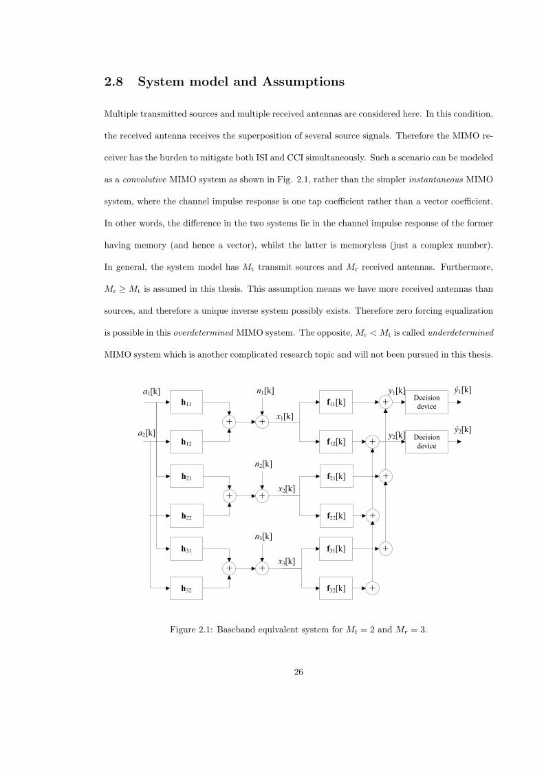
2.8 System model and Assumptions
Multiple transmitted sources and multiple received antennas are considered here. In this condition,
the received antenna receives the superposition of several source signals. Therefore the MIMO re-
ceiver has the burden to mitigate both ISI and CCI simultaneously. Such a scenario can be modeled
as a convolutive MIMO system as shown in Fig. 2.1, rather than the simpler instantaneous MIMO
system, where the channel impulse response is one tap coefficient rather than a vector coefficient.
In other words, the difference in the two systems lie in the channel impulse response of the former
having memory (and hence a vector), whilst the latter is memoryless (just a complex number).
In general, the system model has Mt transmit sources and Mr received antennas. Furthermore,
Mr ≥Mt is assumed in this thesis. This assumption means we have more received antennas than
sources, and therefore a unique inverse system possibly exists. Therefore zero forcing equalization
is possible in this overdetermined MIMO system. The opposite,Mr < Mt is called underdetermined
MIMO system which is another complicated research topic and will not been pursued in this thesis.
h11
a1[k]
f11[k]
+
h12
Decision
device
f12[k]Decision
device
+
+a2[k]
x1[k]
y1[k]
y2[k]
ŷ1[k]
ŷ2[k]
h21 f21[k]
+
h22 f22[k]
+
+
x2[k]
h31 f31[k]
+
h32 f32[k]
+
+
x3[k]
+
n1[k]
+
n2[k]
+
n3[k]
Figure 2.1: Baseband equivalent system for Mt = 2 and Mr = 3.
26
The underdetermined MIMO system is complicated because its inverse system is ambiguous from
a mathematical perspective [105]. Finally, we highlight that the trivial case ofMr = 1 andMt = 1,
the system model is reduced to a convolutive SISO system model.
We further make the following assumptions, which are common:
A1 Assumption on sources:
The j-th source, aj [k], where j ∈ (1,Mt), is an independently and identically distributed
(i.i.d.) zero mean discrete time sequence. All sources, aj [k], j ∈ (1,Mt) are uniformly selected
from a PAM or QAM alphabet set, A and therefore aj [k] has zero mean, Eaj [k] = 0, a
finite power, σ2A = E|aj [k]|2 > 0 and a finite fourth order moment, m4 = E|aj [k]|4 > 0
where E· denotes statistical expectation. Since aj [k] is uniformly picked from a PAM or
QAM alphabet set, aj [k] is circular and sub-Gaussian. Therefore, its normalized kurtosis,
Kur , m4
σ4A
must satisfy Kur < 3 for real-valued case [2] and Kur < 2 for complex-valued case
[36]. In addition, aj [k] and al[k + δ], where δ ∈ Z is any integer, l = j and 1 ≤ l ≤ Mt, are
mutually independent so that
Eaj [k]a∗l [k + δ] = Eaj [k]Ea∗l [k + δ] = 0 (2.1)
where ∗ denotes complex conjugate.
A2 Assumption on channels:
We model the channels from j-th input to i-th channel output as static finite impulse response
(FIR) vectors and denote them as hij = [hij [0], hij [1], · · · , hij [Nh − 1]]T, where i ∈ (1,Mr),
j ∈ (1,Mt), and all channels have the same length, Nh. The properties and descriptions
of channel are stated below. First, the channel is modeled as FIR vector because we focus
on a stable bounded-input bounded-output channel which possibly allows a stable inverse
system to be exist. Second, the channel is modeled as Nh length FIR vectors because we
assume the channel has memory due to multipath propagation. This type of channel is called
frequency selective channel which causes ISI. Third, the channels, which is FIR vectors, can
27
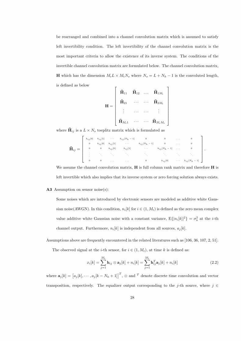
be rearranged and combined into a channel convolution matrix which is assumed to satisfy
left invertibility condition. The left invertibility of the channel convolution matrix is the
most important criteria to allow the existence of its inverse system. The conditions of the
invertible channel convolution matrix are formulated below. The channel convolution matrix,
H which has the dimension MrL×MtNs where Ns = L+Nh − 1 is the convoluted length,
is defined as below
H =
H11 H12 . . . H1Mt
H21 · · · · · · H2Mt
... · · · · · ·...
HMr1 · · · · · · HMrMt
where Hij is a L×Ns toeplitz matrix which is formulated as
Hij =
hij [0] hij [1] · · · hij [Nh − 1] 0 0 . . . 0
0 hij [0] hij [1] · · · hij [Nh − 1] 0 . . . 0
0 0 hij [0] hij [1] · · · hij [Nh − 1] . . . 0
.
.
.
...
...
...
...
...
...
...
0 0 . . . . . . 0 hij [0] · · · hij [Nh − 1]
.We assume the channel convolution matrix, H is full column rank matrix and therefore H is
left invertible which also implies that its inverse system or zero forcing solution always exists.
A3 Assumption on sensor noise(s):
Some noises which are introduced by electronic sensors are modeled as additive white Gaus-
sian noise(AWGN). In this condition, ni[k] for i ∈ (1,Mt) is defined as the zero mean complex
value additive white Gaussian noise with a constant variance, E|ni[k]|2 = σ2n at the i-th
channel output. Furthermore, ni[k] is independent from all sources, aj [k].
Assumptions above are frequently encountered in the related literatures such as [106, 36, 107, 2, 51].
The observed signal at the i-th sensor, for i ∈ (1,Mr), at time k is defined as:
xi[k] =
Mt∑j=1
hij ⊗ aj [k] + ni[k] =
Mt∑j=1
hTijaj [k] + ni[k] (2.2)
where aj [k] =[aj [k], · · · , aj [k −Nh + 1]
]T, ⊗ and T denote discrete time convolution and vector
transposition, respectively. The equalizer output corresponding to the j-th source, where j ∈
28
(1,Mt), at time k is denoted as:
yj [k] =
Mr∑i=1
fTij [k]xi[k] (2.3)
where xi[k] = [xi[k], · · · , xi[k − L+ 1]]T is the input regressor vector for the equalizers of the i-th
seonsor (there are a total of Mt equalizers associated with each of the i sensors), L is sufficiently
large to eliminate the ISI of the channel, and fij [k] =[f[0]ij [k], · · · , f [L−1]
ij [k]]T
is a L×1 vector that
represents the equalizer connecting the observed signal at i-th sensor to the j-th equalizer output
at time k. There are a total of Mt ·Mr equalizers at the receiver end (see Fig. 2.1). Furthermore,
Eq. 2.3 can be written as
yj [k] = FTj [k]X[k] (2.4)
where Fj [k] =[fT1j [k], · · · , fTMrj
[k]]T
is a MrL × 1 vector and X[k] =[xT1 [k], · · · ,xT
Mr[k]]T
is a
MrL× 1 vector.
Then, yj [k] is fed into decision device and the decision device generates yj [k]. yj [k] is chosen
based on yj [k] and the alphabet set, A. A symbol in A which has the smallest Euclidean distance
to yj [k] is chosen as yj [k]. For example in 4-QAM, the relationship between yj [k] and yj [k] is
mathematically expressed as
Reyj [k] =
−1 if Reyj [k] ≤ 0
1 otherwise
(2.5)
and
Imyj [k] =
−1 if Imyj [k] ≤ 0
1 otherwise
(2.6)
29
Another example for 16-QAM, the mathematic relationship between yj [k] and yj [k] is
Reyj [k] =
−3 if Reyj [k] ≤ −2
−1 if −2 < Reyj [k] ≤ 0
1 if 0 < Reyj [k] ≤ 2
3 otherwise
(2.7)
and
Imyj [k] =
−3 if Imyj [k] ≤ −2
−1 if −2 < Imyj [k] ≤ 0
1 if 0 < Imyj [k] ≤ 2
3 otherwise
(2.8)
2.9 Definition of a Good MIMO Blind Equalizer
We are going to mathematically describe a good MIMO blind equalizer that not only suppresses
ISI and CCI but also retrieves all symbol sequences without repetition in the steady state [36].
First, we formulate a global system which combines channels and equalizers into a single system
so that it directly connects input sources to outputs. The pattern of impulse responses in the
global system is the key to determine a MIMO blind equalizer. In short, the suppression of ISI
and CCI doesn’t mean that it has achieved all its objectives, because the same source may be
extracted twice (or more) in the receiver outputs while missing some, which in this case is bad.
This activity is often known as source separation. In what follows we will show in the ideal case
(i.e. equalization and source separation achieved), the global transfer function reduces to a special
type of identity matrix, where the diagonal elements, which are polynomial functions, have only
one non-zero coefficient. While this is achievable with trained systems (i.e. a known training
30
sequence is transmitted along the message signal), blind equalizers can only achieve such a matrix
that is possibly permutated and/or phase rotated.
A good MIMO blind equalizer is one that successfully suppress all ISI, CCI and retrieving all
sources once. In order to show this mathematically, we will pursue it in the Z-domain instead of
time domain because time domain convolution is much more complex and tedious. In the end,
we will get complete source separation and interferences suppression but subject to an ambiguous
permutation and possible phase offset, as seen in the final Eq. 2.16.
To pursue the systems in Z-domain, let us define Unilateral Z-transform of some FIR systems,
such as Unilateral Z-transform of channel hij as
hij(z) =
Nh−1∑p=0
hij [p]z−p (2.9)
and Unilateral Z-transform of equalizer fij [k] as
fij(z) =L−1∑q=0
f[q]ij [k]z−q (2.10)
where fij(z) is assumed has reached the steady state and therefore, it is time k independent. It is
obvious that hij(z) and fij(z) are also polynomial functions which has variable z−1. We further
define aj(z) and yj(z) are Z-transforms of source aj [k] and output yj [k] respectively.
For simplicity, we assume noiseless condition (i.e. σ2n = 0). Without loss of generality, we firstly
assume Mt = 2 transmit sources and Mr = 3 receive sensors. This condition allows us to show the
linear mathematical manipulations of the global system easily. After that, the overall system will
be generalized into any MIMO system and will be described in matrix equation.
With the Mt = 2 and Mr = 3 assumption, the system model in Fig. 2.1 can be decomposed
and split into equalizer 1 and equalizer 2. Fig. 2.2 illustrates the way to form the global transfer
function S(i),j(z) from MIMO channel hij(z) and FIR transfer function fij(z). Fig. 2.2 (i) is
the portion of the model 2.1 that illustrates the relationship between sources (i.e. a1(z) and
a2(z)) and equalizer output, 1 y1(z). The sources transmit signals through MIMO channel which
is represented by MIMO channel transfer function hij(z) for i = 1, 2, 3 and j = 1, 2 where hij(z)
31
represents the channel transfer function that connects source i to the received antenna j. After that,
the MIMO equalizer 1, which is represented by FIR transfer functions f11(z), f21(z) and f31(z),
receives the signal through MIMO channel. f11(z), f21(z) and f31(z) are the FIR transfer functions
that connect received antenna 1, 2 and 3 that belongs to equalizer 1, respectively. The outputs
of the FIR transfer functions are summed up to be equalizer output 1, y1(z). After the sources
and the output are clearly identified, the MIMO transfer function and FIR transfer functions can
be combined into global transfer functions. Fig. 2.2 (ii) illustrates the global transfer functions
S(1),1(z) and S(2),1(z) that are the results of combining MIMO channel transfer functions and FIR
transfer functions, while the sources and output are remained to be unchanged. The correspond
equations of the global transfer functions will be shown later. Similarly, the above descriptions of
Fig. 2.2 (i) and (ii) can be re-used to describe Fig. 2.2 (iii) and (iv) for equalizer 2, instead of
equalizer 1.
From mathematically perspective, y1(z) in Fig. 2.2 (i) can be established as
y1(z) =
=S(1),1(z)︷ ︸︸ ︷(f11(z)h11(z) + f21(z)h21(z) + f31(z)h31(z)
)a1(z)
+
(f11(z)h21(z) + f21(z)h22(z) + f31(z)h32(z)
)︸ ︷︷ ︸
=S(2),1(z)
a2(z)
= S(1),1(z)a1(z) + S(2),1(z)a2(z) (2.11)
where S(i),j(z) is the Z domain global system or is called global transfer function that directly
connects input source i to output j and it is generally defined as
S(i),j(z) =
Mr∑p=1
fpj(z)hpi(z) =
Ns−1∑r=0
S[r](i),jz
−r (2.12)
and due to the reason that fpj(z) and hpi(z) are polynomial functions, the final result of S(i),j(z) is
also a polynomial function with coefficients S[r](i),j and the highest orderNs−1 whereNs = L+Nh−1
is the convolution length. After that, we re-apply the same manipulations to output 2, y2(z), we
32
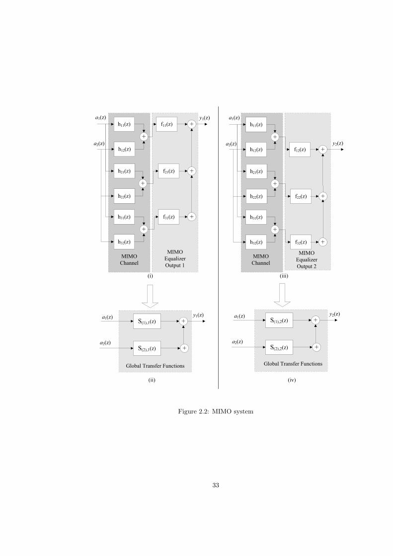
h11(z)
a1(z)
f11(z)
+
h12(z)
+
a2(z)
y1(z)
h21(z) f21(z)
+
h22(z)
+
h31(z) f31(z)
+
h32(z)
+
h11(z)
a1(z)
+
h12(z) f12(z) +a2(z) y2(z)
h21(z)
+
h22(z) f22(z) +
h31(z)
+
h32(z) f32(z) +
(i) (iii)
MIMO
Channel
MIMO
Equalizer
Output 1
MIMO
Channel
MIMO
Equalizer
Output 2
a1(z)S(1),1(z) +
a2(z)+
(ii)
S(2),1(z)
y1(z) a1(z)S(1),2(z) +
a2(z)+S(2),2(z)
y2(z)
Global Transfer Functions Global Transfer Functions
(iv)
Figure 2.2: MIMO system
33
eventually obtain
y2(z) =
=S(1),2(z)︷ ︸︸ ︷(f12(z)h11(z) + f22(z)h21(z) + f32(z)h31(z) ) a1(z)
+ (f12(z)h21(z) + f22(z)h22(z) + f32(z)h32(z) )︸ ︷︷ ︸=S(2),2(z)
a2(z)
= S(1),2(z)a1(z) + S(2),2(z)a2(z) (2.13)
. The role of global transfer functions S(i),j(z) are illustrated in Fig. 2.2 (ii) and (iv) for output 1
and 2 respectively. It is worth to mention that Equations 2.11 and 2.13 are linear functions and
therefore they can be combined into a matrix equation in which the role of equalizer fij(z) can be
easily identified in the matrix equation.
In order to generalize the condition above to Mt transmit sources and Mr receive sensors, we
can form matrix equation below,
y(z) = FT(z)H(z)a(z) = ST(z)a(z) (2.14)
where ()T denotes matrix transpose, F(z) is a Mr×Mt polynomial matrix that describes equalizer
transfer functions and is defined as
F(z) =
f11(z) f12(z) · · · f1Mt(z)
f21(z) f22(z)... f2Mt(z)
......
......
fMr1(z) · · · · · · fMrMt(z)
,
H(z) is a Mr ×Mt polynomial matrix that describes channel transfer functions and is defined as
H(z) =
h11(z) h12(z) · · · h1Mt(z)
h21(z) h22(z)... h2Mt(z)
......
......
hMr1(z) · · · · · · hMrMt(z)
.
Furthermore, S(z) is a Mt ×Mt polynomial matrix. It describes global transfer functions which
34
combines channel and equalizer transfer functions and is defined as
S(z) =
S(1),1(z) S(1),2(z) · · · S(1),Mt(z)
S(2),1(z) S(2),2(z)... S(2),Mt(z)
......
......
S(Mt),1(z) · · · · · · S(Mt),Mt(z)
.
Finally, a(z) = [a1(z), a2(z), . . . , aMt(z)]T and y(z) = [y1(z), y2(z), . . . , yMt(z)]
T are Mt × 1
polynomial matrices which represent Z-transform of input sources and outputs respectively.
Ideally, to recover all source sequences without any interferences, the equalizer matrix F(z) in
Eq. 2.14 is chosen, so that the global matrix, S(z) should satisfy,
S(z) = HT(z)F(z) = diag(z−d1 , z−d2 , . . . , z−dMt ) (2.15)
where diag(z−d1 , z−d2 , . . . , z−dMt ) denotes a Mt × Mt diagonal matrix and d1, d2, . . . , dMt ∈
0, 1, . . . , Ns − 1. Eq. 2.15 implies that the output j may retrieves the dj time delay version
of symbol sequence from source j where j = 1, . . . ,Mt. However, the ideal solution in Eq. 2.15
cannot be achieved in MIMO blind equalization since the exact source sequences and the position
j of source are unknown by the receiver. Therefore, output j does not always retrieve input source
j and this weakness is called permutation ambiguity. Instead of that, due to the statistical cir-
cular symmetry condition on input sources, MIMO blind equalization cannot identify the phase
of sources and this problem is called phase ambiguity. Hence, the best possible solution that is
provided by MIMO blind equalization is
S(z) = HT(z)F(z) = diag(ejθd1 z−d1 , ejθd2 z−d2 , . . . , ejθdMt z−dMt )P (2.16)
where P is a permutation matrix and ejθdn denotes any possible phase offset with −π ≤ θdn < π,
j =√−1 and n = 1, . . . ,Mt. Thus, a good MIMO blind equalizer should satisfy Eq. 2.16 which
retrieves all source sequences and suppresses interferences but includes permutation ambiguity and
phase ambiguity.
35
2.10 Time Domain Identification of Good MIMO Equalizer
(with examples)
The Z domain matrix form in previous section may be difficult to visualize. Therefore we will
provide the equivalent presentation in the time-domain vector form. We will present the absolute
global impulse responses which are formed by the coefficient magnitudes of global transfer functions.
Furthermore, the absolute global impulse responses are widely been used as the tool to identify a
good equalizer in the steady state [36]. This section is structured as follows. First, we describe the
global impulse response which is the time domain counterpart of global transfer function. Then,
we present the absolute global impulse responses that are magnitude version of global impulse
response and does not depend on phase.
The global impulse response, S(i),j [k] that connects input source i with output j is the inverse
Z transform of the global transfer function S(i),j(z) in which S(i),j [k] is a Ns × 1 vector and is
defined as
S(i),j [k] =
[S[0](i),j , S
[1](i),j , . . . , S
[Ns−1](i),j
]T. (2.17)
It is obvious to see that the r+1-th element in S(i),j [k] above is the coefficient S[r](i),j that belongs to
variable z−r in S(i),j(z) (see Eq. 2.12). Therefore, the global impulse response S(i),j [k] is a straight
forward transformation from the global transfer function S(i),j(z). Due to phase ambiguity issue in
blind equalizer, the result of coefficient S[0](i),j is subject to phase ambiguity as well. For simplicity,
we observe the magnitude of coefficient S[0](i),j , |S
[0](i),j | which does not depend on phase. In this
condition, the absolute global impulse response, |S(i),j [k]| where
|S(i),j [k]| =[|S[0]
(i),j |, |S[1](i),j |, . . . , |S
[Ns−1](i),j |
]T(2.18)
which only computes coefficient magnitude.
The success of a MIMO equalizer can be visually determined by observing the coefficients of
|S(i),j [k]| in the steady state. In particular, we look for source retrieval of the intended source and
36
source suppression for the neighbor sources. To demonstrate how we judge the success of a MIMO
equalizer, we provide the following 3 examples which utilizes a simple Mt = 2 MIMO equalizer.
2.10.0.1 Example 1: Good MIMO Equalizer
A good MIMO equalizer would generate an impulse for |S(1),1[k]| and |S(2),2[k]|, as well as an
all-zero vector for |S(2),1[k]| and |S(1),2[k]| at steady state. For example this set of |S(i),j [k|]
vectors implies our objectives of equalization and source separation are met: |S(1),1[k]| = [0, 0, 1, 0],
|S(2),1[k]| = [0, 0, 0, 0], |S(1),2[k]| = [0, 0, 0, 0] and |S(2),2[k]| = [0, 0, 0, 1].
Let us firstly consider S(1),1[k] and S(2),1[k]. The single impulse in the 3rd coefficient in S(1),1[k]
implies perfect equalization of source 1 but delayed by 2 symbol periods, i.e. the retrieval of
|a1[k − 2]|. It also means source 2 is completely suppressed at the output of equalizer 1.
In a similar fashion, the all-zero S(1),2[k] and the single impulse S(2),2[k] implies the successful
retrieval of source 2 and suppression of source 1 at the output equalizer 2.
Therefore, y1[k] retrieves the symbol sequence from source 1 alone and y2[k] from source 2
alone, albeit being delayed, which does not affect the bit error rate performance. We consider this
as a completely successful MIMO equalization.
2.10.0.2 Example 2: Good MIMO Equalizer with source permutation
We consider another good case where |S(1),1[k]| = [0, 0, 0, 0], |S(2),1[k]| = [0, 1, 0, 0], |S(1),2[k]| =
[0, 0, 1, 0] and |S(2),2[k]| = [0, 0, 0, 0] in the steady state. Using the same explanation in Example 1,
here y1[k] retrieves source 2 while y2[k] retrieves source 1. Therefore source permutation is present,
but this can be easily resolved and therefore this setting is considered successful.
2.10.0.3 Example 3: MIMO Equalizer with source separation failed
We consider an unsuccessful case where |S(1),1[k]| = [0, 1, 0, 0], |S(2),1[k]| = [0, 0, 0, 0], |S(1),2[k]| =
[0, 0, 1, 0] and |S(2),2[k]| = [0, 0, 0, 0] in the steady state.
37
Here, it can be seen that both equalizers retrieve the same source, i.e. source 1, thus missing
source 2 entirely. This is an example of retrieving the same source repeatedly and missing at least
one other source. Although the ISI has been successfully mitigated, we do not consider this as a
successful MIMO equalizer.
2.11 The way of adaptation in MIMO equalizer
We briefly describe the way of a MIMO equalizer adapts in this section. We recall Eq. 2.16 and
then we define a good MIMO equalizer to have the optimum transfer function Fopt(z). Therefore,
Fopt(z) should satisfy
Sopt(z) = HT(z)Fopt(z) = diag(ejθd1 z−d1 , ejθd2 z−d2 , . . . , ejθdMt z−dMt )P (2.19)
where Sopt(z) is the optimum global transfer function that indicates a good equalization has been
achieved. Furthermore, we define the time domain counterpart of Fopt(z) as Fopt[k], which is the
impulse responses of MIMO equalizer, and is defined as
Fopt[k] =
[FT
1,opt[k],FT2,opt[k], . . . ,F
TMr,opt[k]
]T(2.20)
where FTj,opt[k] is the optimum equalizer for output j.
In order to achieve the above optimum condition in the steady state, it is obvious that the
equalizer j, Fj [k] should be adapted by an algorithm towards its optimum Fj,opt[k], which is
a static value. The above adaptation process can be done by an optimization algorithm which
normally achieves optimum situation by minimizing a non-zero real function. In the literature,
stochastic gradient descent algorithm (SGA) is widely been chosen as the optimization algorithm
because of its simplicity in hardware implementation. Ideally, SGA searches for a minimum point of
an user-defined non-negative function, which is called cost function. After SGA found a minimum
point of the cost function, SGA will stay steadily on the minimum point. Therefore, researchers
normally design a cost function that is a function of multivariate Fj [k] and locate the global
minimum of the cost function on the multivariate optimum value Fj,opt[k].
38
In practice, Fj [k] is initialized on any value Fj [0] that corresponds to a non-minimum point in
the cost function. After that, Fj [k] is started to be iteratively adapted by SGA towards Fj,opt[k].
Eventually, when Fj [k] ≃ Fj,opt[k] happened, the value Fj [k] is expected to be unchanged by SGA
since the steady state is reached. This condition is called global convergence because the MIMO
equalizer converges to the global minimum point and a good MIMO equalizer is achieved.
However, due to the reason that some cost functions have local minima, SGA possibly causes
Fj [k] to stay steadily on the local minima instead of the global minimum if certain criterions have
not been fulfilled. If so, this situation is known as ill-convergence or local convergence because the
equalizer converges to a local minimum point instead of the global minimum point. This implies
MIMO equalization is unsuccessful.
In the literature, many SISO and MIMO blind equalization algorithms are developed based
on SGA . Generally, these algorithms can be categorized into robust algorithm and non-robust
algorithm. Robust algorithm is a blind equalization algorithm that has avoidable local minima.
This means equalizer possibly converges to the global minima if suitable parameters are chosen.
On the other hand, non-robust algorithm is a blind equalization algorithm that has unavoidable
local minima. Robust and non-robust algorithms will be reviewed in Section 2.13-2.15.
2.12 Performance Measurements
The absolute global impulse responses in the previous section are effective tools to identify a good
MIMO equalizer that achieves ISI and CCI suppression. The performance of such a good MIMO
equalizer can be measured using either the residual interference of the equalizer output j (ITj [k])
or the mean square error (MSE) of output j (MSEj [k]). They are commonly used performance
measurements in the literature and will be adopted in this thesis. MSEj [k] measures the residual
interference with the aid of decision device and it is suitable to be used in the presence of AWGN
noise. On the other hand, ITj [k] evaluates the amount of residual interference based on global
impulse responses without the presence of AWGN noise but it requires knowledge of the channel
39
which is often absent in real implementation (although in simulation environments we usually
have accessed to the channel). In fact, a low value of ITj [k] or MSEj [k] is always desired as
it reflects good equalizer quality. Instead of that, ITj [k] is insensitive to the scale because it
is normalized by the largest amplitude. In contrary, no normalized operation has been done on
MSEj [k], therefore MSEj [k] can be used to trace the presence of scale. Here we emphasize that
although ITj [k] or MSEj [k] may be low, source separation might not have been attained so the
technique of absolute global impulse response (outlined in Section 2.4) is always needed to first
determine source separation.
First, the amount of residual interference of the equalizer outputs for the j-th equalizer output
at time instant k, ITj [k] is defined as below [36]
ITj [k] = 10 log10
Mt∑i=1
Ns−1∑n=0
∣∣∣s[n]ij [k]∣∣∣2 −maxi,n
∣∣∣s[n]ij [k]∣∣∣2
maxi,n
∣∣∣s[n]ij [k]∣∣∣2
(2.21)
where s[n]ij [k] is the (n + 1)-th element of the global impulse response S(i),j [k], S(i),j [k] being the
global impulse response that connects the i-th source, ai[k], to yj [k] and maxi,n∣∣s[n]ij [k]
∣∣2 is a
function that selects the largest value of |s[n]ij [k]|2 in 0 ≤ n ≤ Ns − 1 and 1 ≤ i ≤Mt.
Next, MSE of the j-th equalizer output, MSEj [k] is computed as following,
MSEj [k] = 0.99MSEj [k − 1] + 0.01 |yj [k]− yj [k]|2 (2.22)
where yj [k] denotes the output of decision device and MSEj [0] = 1 is initialized. Furthermore,
MSE in decibel (dB) unit is defined as MSEj [k] (dB) = 10log10MSEj [k].
2.13 Review on SISO Blind Equalization Algorithms
Since 1960s, many blind equalization algorithms have been developed for SISO system to suppress
ISI from a frequency selective channel. It is worth to mention that the development of MIMO blind
equalization algorithm are normally inherent the concept or idea of SISO blind equalization algo-
rithm. Therefore, it is important to review some famous SISO blind equalization algorithms such
40
as Decision Directed (DD) algorithm [108], Sato algorithm [22] and Gordard algorithm or Constant
Modulus algorithm (CMA) [21] in this section. The main differences among these algorithms lie in
their cost functions. In the following, we will briefly review how does the previous works categorize
the above algorithms into robust or non-robust algorithms. After that, each algorithms and their
uniqueness will be presented.
All blind equalization algorithms have undesirable local minima in its global response (i.e. the
combination of channel and equalizer) cost surface if the FIR filter (i.e. Assumption A2) is used to
model both the channel and the equalizer [109]. If the coefficients of the equalizer converge to these
local minima, the ISI will not be suppressed successfully. Therefore, a blind algorithm that has
the fewest distinct local minima is widely preferred since it reduces the risk of local convergence.
It is worth to mention that Li et al [109, 110, 111] had analyzed some popular algorithms and
found that local minima in CMA can be avoided if correct parameters are chosen at the initial
stage. Based on this reason, we categorize CMA as a robust algorithm. Furthermore, the same
analysis performed on the Sato algorithm and the DD algorithm show that they too have many
local minima, so the local convergence problem is more likely encountered in implementation. Due
to this reason, we categorize the Sato and the DD algorithms as non-robust algorithms, make the
CMA (or more generally known as the Godard algorithm) the first even robust blind equalization
algorithm that was developed.
Next, we explain the cost function of an algorithm, before reviewing its place in the stochastic
gradient algorithm (SGA) which is widely used due to its simplicity.
Generally, blind equalization algorithms are derived based on a non-negative cost function
which has a general form,
J1[k] = E|ε1[k]|2
(2.23)
where J1[k] is the cost function of equalizer output 1 and ε1[k] is called error function of equalizer
output 1 which is different for each algorithms. However, E|ε1[k]|2
in Eq. 2.23 is impossible
to be directly determined in real implementation due to the E. operator. Therefore, the past
41
literature normally estimate E. using an instantaneous value. This estimation method does not
introduce additional offset and therefore it is an unbiased estimation [112, 113, 114]. Therefore,
the estimation of the cost function becomes
J1[k] , |ε1[k]|2. (2.24)
After that, stochastic gradient descent algorithm (SGA) is applied to find the minimum point of
the cost function in Eq. 2.24. After incorporating with SGA, the tap coefficients, F1[k] have a
general update equation,
F1[k + 1] = F1[k]− µ1∂
∂F1[k]J1[k]
= F1[k]− µ1ε1[k]X∗[k] (2.25)
where F1[k] and X[k] were defined in Section 2.8, µ1 is user-defined step size and ∂∂F1[k]
J1[k] is the
gradient of the cost function J1[k] (Note: the algebraic manipulation of ∂∂F1[k]
J1[k] can be found
in some popular books such as [115, 116, 117] or calculus books).
First, we review the DD algorithm [108] which is the simplest algorithm. The error function of
the DD algorithm is
ε1[k] = y1[k]− y1[k] (2.26)
where y1[k] is the decision output and is shown in Section 2.8. The DD algorithm is poor to open
the channel eye because the decision output, y1[k] is always unreliable in the closed eye condition.
Therefore, the DD algorithm, which is a non-robust algorithm, is easy converge to local minima. In
practice, the DD algorithm is used after the channel eye is opened because the decision output y1[k]
is only reliable in open eye conditions. Furthermore, in an open eye condition, the DD algorithm
can provide the lowest MSE in comparison with the Sato algorithm and the CMA.
Sato algorithm [22] has widely been recognized as the first blind equalization algorithm because
it is the first algorithm that can open the channel eye. However, the open eye ability of Sato
algorithm is restricted to minimum phase channels. Due to the reason that Sato algorithm only
exploits the second order statistic, it cannot distinguish between common magnitude response
42
channels such as a + bz−1 or b + az−1 [114]. Therefore, the algorithm is not able to open the
non-minimum phase channel eye [118] because Sato algorithm mistakenly assumes the channel is a
minimum phase channel. As a result, Sato algorithm equalizes the magnitude response of the non-
minimum phase channel but it wrongly equalizes the phase response of the non-minimum phase
channel. This implies that Sato algorithm will often converge to a spurious local minimum when
the channel is the non-minimum phase channel. Hence, Sato algorithm is a non-robust algorithm
since it cannot avoid local convergence for the non-minimum phase channel due to imperfect cost
function regardless of parameters. The error function of Sato algorithm for implementation is given
as
ε1[k] = (|y1[k]| − RSato) (2.27)
where RSato = E|a1[k]|2/E|a1[k]|.
To overcome the above problem, Godard has generalized Sato algorithm to take into account
high order statistics and the generalized algorithm is called Godard algorithm [21]. Godard al-
gorithm with fourth order statistic has been proven to successfully open the eye of even a non-
minimum phase channel. At the same time, J. R. Treichler [119] independently proposed Constant
Modulus Algorithm (CMA) which is exactly same as Godard algorithm with fourth order statis-
tic. Therefore, CMA is also known as Godard algorithm. Subsequently, due to the widespread
popularity of the CMA, its convergence behavior is thoroughly and exhaustively studied in [120],
[109], [121], [122], [123] and [114]. These studies have identified the ill-convergence factors in
CMA and proposed many solutions. Some important studies by [120] and [109] have found that
proper filter taps initialization with a sufficiently small step size and at least one non-zero value
in tap coefficients can avoid the occurrence of ill-convergence . This is because the previous works
had identified the only undesired local minima of CMA is the origin, so initializing the otherwise
all-zero equalizer coefficient vector with a single non-zero value is helpful to lead the equalizer
“far away” from this specific undesirable local minimum at origin. As a result, CMA has widely
been recognized as a good candidate for blind equalization since risks on CMA have been clearly
43
identified and effectively mitigated by the above studies. Generally, the cost function of the CMA
is
J1[k] = E
(|y1[k]|2 − R1
)2(2.28)
where R1 = E|a1[k]|4/E|a1[k]|2 is the dispersion constant for equalizer output 1. However, the
expectation value E. is unknown in practice, therefore the cost function of the CMA is widely
estimated as
J1[k] ,(|y1[k]|2 − R1
)2(2.29)
where the instantaneous sample value is used to estimate its expectation value E.. Finally, the
error function of the CMA for implementation is given as
ε1[k] = y1[k](|y1[k]|2 − R1
). (2.30)
Even though the global convergence of CMA was confirmed, CMA have some drawbacks in
the quality. The drawbacks of CMA are low convergence rate and high steady state MSE for
multi-modulus source symbol such as 16-QAM [54] [123]. To hasten the convergence and reduce
the steady state MSE, hybrid algorithms (explained in the section below) which combine CMA
and DD algorithm have been proposed.
2.14 Review on SISO Hybrid Algorithms
A hybrid algorithm that is employed by the equalizer is called that way because it opens the channel
eye using an acquisition algorithm, for example CMA, and tracks the channel (after the channel
eye is open) using a DD algorithm. The acquisition algorithm is capable of opening the channel eye
provided sufficiently small adaptation step size but usually yields large steady state errors [123],
[21], [22],[120] and normally a robust algorithm will be selected as acquisition algorithm. That
is why hybrid algorithms couple the acquisition algorithm with a tracking algorithm (e.g. DD
algorithm) to exploit the discrete nature of the input data to achieve much lower error rates. Hybrid
44
algorithms include Stop-And-Go Algorithm Decision Directed Algorithm (SAG) [124], Benveniste-
Goursat Algorithm (BG) [125] and Reliability Based Algorithm (RBA)[126].
The error function, ε1[k] (in Eq. 2.24) is a function of ϵacq[k] and ϵtr[k] where ϵacq[k] and
ϵtr[k] are defined as the blind equalization error function for the acquisition mode and the tracking
mode at time instant k respectively. In the literature, CMA is selected as the choice of the
acquisition algorithm since CMA is a good open eye blind algorithm, while DD algorithm is used
as the tracking algorithm because DD algorithm yields a very low steady state MSE. Therefore,
ϵacq[k] = y1[k](|y1[k]|2 − R1
)and ϵtr[k] = y1[k]− y1[k] are established.
2.14.1 Stop-And-Go Algorithm Decision Directed Algorithm (SAG)
SAG is introduced by [124] with the real and imaginary part of equalization error function below:
Reε1[k] =
γSAGReϵtr[k] if sgn (Reϵtr[k]) = sgn (Reϵacq[k])
0 otherwise
(2.31)
and
Imε1[k] =
γSAGImϵtr[k] if sgn (Imϵtr[k]) = sgn (Imϵacq[k])
0 otherwise
(2.32)
where Re. and Im. denote real part and imaginary part respectively, sgn(.) is a signum function
and γSAG is a positive constant. SAG relies on the same gradient descent direction of the acquisition
algorithm and the tracking algorithm (i.e. sgn (ϵtr[k]) = sgn (ϵacq[k])) to approach the minimum
point. The equalization error is updated if the matched sign condition happened, otherwise, no
updated on tap coefficient is required. This means SAG updates error function only when the error
function is reliable. According to Lim et al [127], SAG is the slowest hybrid algorithm because the
tap is not updated every iteration. However, SAG give the best quality in the steady state since
it provides the lowest mean square error MSE.
45
2.14.2 Benveniste-Goursat Algorithm (BG)
Benveniste et al [125] suggested the first smooth transition hybrid method with the following
equalization error function:
ε1[k] = β1∣∣ϵtr[k]∣∣ϵacq[k] + β2ϵtr[k] (2.33)
where β1 and β2 are positive constants. BG provides a smooth transition between the acquisition
algorithm and the tracking algorithm. The term β1∣∣ϵtr[k]∣∣ determines the weight of the acquisition
algorithm. From Eq. (2.33), BG yields larger error function since it is always occupied by two
terms rather than one term, ϵtr[k] in SAG. Therefore, it has higher MSE than SAG [127].
2.14.3 Reliability Based Algorithm (RBA)
The above algorithms decide the switching criteria between the acquisition algorithm and the
tracking algorithm based on a single factor - the instantaneous value of ϵtr[k]. Based on the reason
that the instantaneous value does not exactly reflect the channel eye at the onset of equalization,
false switching to the tracking algorithm in the closed eye condition may occur and may reduces
the convergence rate. Hence, Lim et al [126] suggested the switching criteria is not only depends
on the instantaneous value but also take into account of the chances of correct output and based
on maximum a posteriori (MAP) criterion. The chances of the correct output are known as the
probability of correctly detecting a symbol for the output at time instant k, Pc[k]. Generally,
this method has higher computation cost but it outperforms the other methods. We denote this
method as RBA and the equalization error function is below:
ε1[k] = (1− α[k]) ϵacq[k] + α[k]γRBAϵtr[k] (2.34)
where γRBA is a positive constant and α[k] is defined as below after some modification:
α[k] =
0 if Pc[k] < Pth or σ2[k] > σ2
th
2Pc,j [k]− 1 otherwise
46
where Pth and σ2th are the positive constant and Pc,j is defined as below:
Pc[k] =
exp
(−∣∣y[k]−y1[k]
∣∣2σ2[k]
)NQAM∑t=1
exp
(−∣∣y[k]−At)
∣∣2σ2[k]
) (2.35)
where At is the tth constellation point in the NQAM QAM alphabet set A and σ2[k] is the variance
of y[k]. The estimation of σ2[k] in practice, σ2[k] (with σ2[0] = 10) as below:
σ2[k] = 0.99σ2[k − 1] + 0.01 |y[k]− y1[k]|2 (2.36)
2.15 MIMO Blind equalization and source separation algo-
rithms
The suppression of ISI and CCI in the conventional blind equalization is useful to open the channel
eye, but it does not imply the receiver can retrieve all the transmitted sources. This is because
the receiver has the chance to recover at least two similar symbol sequences and thus the receiver
probably misses to recover some sources. In order to overcome this, blind equalization that is
equipped with source separation ability is required. However, in the previous works, many types
of blind equalization algorithms have been developed but not all algorithms are equipped with
source separation ability. In order to identify this type algorithm, we divide the blind equalization
algorithms into 4 types based on the presented simulation results.
• Source separation algorithm: It is a blind algorithm that can perform source separation
but is designed and tested solely in CCI without ISI. This algorithm also known as blind
source separation (BSS).
• Pure equalization algorithm: It is a blind algorithm that can suppress interferences but
cannot perform source separation.
• Single task algorithm: It is a blind algorithm that can perform solely one task in a time,
either equalization or source separation but not the both.
47
• Two tasks algorithm: It is a blind algorithm that can perform two tasks of equalization
and source separation simultaneously.
Obviously, the two tasks algorithm is the algorithm that we are interested. Therefore, this type
algorithm will be focused and reviewed later. Instead of that, source separation algorithm, pure
equalization algorithm and single task algorithm will be briefly reviewed as follows.
2.15.1 Source separation algorithm
This type algorithm is designed based on the assumption of memoryless MIMO channels where
Nh = 1 , and thus only CCI is considered in the model. In order to recover a source signal
from CCI, source separation algorithm is used. In fact, based on the implementation method, the
algorithm can be divided into batch algorithm and adaptive algorithm. Batch algorithm updates
the filter coefficients after the receiver obtains certain number of symbols. On the contrary, the
adaptive algorithm updates the filter coefficients when a symbol is received. Therefore, the adaptive
algorithm is a real time instantaneous algorithm and produces output immediately. However, the
batch algorithm typically computes average on a batch of symbols, therefore the batch algorithm
is less susceptible to noise. Examples of batch algorithm and adaptive algorithm are described as
follows.
Principle Component Analysis (PCA), Factor Analysis (FA) [26] and Independent Component
Analysis (ICA) [27, 28, 29] are the examples of batch source separation algorithm. PCA and FA are
second order statistic algorithms that are used to perform uncorrelated pre-processing. However,
These pre-processing algorithms cannot perform well in severe corrupted channel, therefore, high
order statistics algorithm such as ICA is always appended after the pre-processing algorithm. In
contrast to the pre-processing algorithms, ICA is an algorithm to ensure the receiver outputs are
mutually independent. ICA can be achieved by maximizing a kurtosis cost function or a negative
entropy cost function. Maximizing the kurtosis cost function can ensure the outputs becomes
less statistical“Gaussainity” and thereby increases the independency among the outputs. On the
48
contrary, maximizing the negative entropy increases the statistical “uniformly” of the outputs
and thus increases the independency among the outputs. These two cost functions achieve the
independency through changing the output density functions. Due to the reason that the original
information sources are i.i.d. , which is a special case of uniform distribution, the negative entropy
cost function can perform better than kurtosis cost function. However, because of unknown source
signals, ICA has the limitations of scale and permutation ambiguities [30].
Instead of that, Blind Source Separation Constant Modulus Algorithm (BSS-CMA) [31], Blind
Source Separation Multi Modulus Algorithm (BSS-MMA) [32], Orthogonal Multi Modulus Algo-
rithm (O-MMA) [33], Cross-Correlation Simplified Constant Modulus Algorithm (CC-SCMA) [34]
are the adaptive source separation algorithms that can be found.
Blind Source Separation Constant Modulus Algorithm (BSS-CMA), which is directly adopted
from SISO CMA and applied in memoryless MIMO channels, can show the ability of open eye
in CCI distortion but it has some issues in permutation ambiguity, computation complexity, con-
vergence rate and steady state performance [31]. Therefore, several solutions are proposed to
overcome the issues. Blind Source Separation Multi Modulus Algorithm (BSS-MMA) is intro-
duced to reduce the infinite permutation ambiguity to modulo 90 degree phase ambiguity [32]. By
enhancing BSS-MMA, Orthogonal Multi Modulus Algorithm (O-MMA) has been proposed. Dif-
ferent with BSS-MMA and BSS-CMA, Orthogonal Multi Modulus Algorithm (O-MMA) has lower
computation complexity and an orthogonal constrained on the filter to ensure the outputs are
always mutually orthogonal, thereby the source separation performance is better than BSS-MMA
[33]. Instead of that, Cross-Correlation Simplified Constant Modulus Algorithm (CC-SCMA) [34]
is developed to improve the steady state performance of BSS-CMA. However, these algorithms has
been developed under the assumption of invertible channels. The performance of the algorithms
in non-invertible channels is unknown.
Nevertheless, due to the ISI has not been considered, the source separation algorithm is not a
good choice for MIMO equalization.
49
2.15.2 Pure equalization algorithm
This is a classical algorithm that was design for convolutive MIMO channel where Nh > 1. In this
case, the receiver obtains the signals that have been corrupted by ISI and CCI. Therefore, in order
to suppress the interferences, MIMO-CMA where CMA in SISO system was adopted and applied
in MIMO equalizer [35] [36]. The MIMO-CMA can open the channel eye of the convolutive MIMO
channel but its source separation ability is not guaranteed because the same source sequence is
possibly recovered more than one time at the equalizer outputs [36]. Therefore, this type algorithm
is not a good candidate for MIMO equalization. To overcome this issue, single task algorithm and
two tasks algorithm are developed.
2.15.3 Single task algorithm
This type of algorithm can only one task in a time. It can be only used for blind equalization
or blind source separation, but not for both cases. To the best of the author’s knowledge only
two algorithms can be found. One is second order quadratic programming approach [37] and the
other one is high order statistics approach [38]. Nevertheless, due to this type algorithm cannot
perform equalization and source separation simultaneously, it is not a good candidate for MIMO
equalization.
2.15.4 Two tasks algorithm
Two tasks algorithm is aimed to perform equalization and source separation at the same time. In
general, the tasks can be achieved through orthogonal constraint cost function approach or non-
constraint cost function approach. Non-constraint cost function approach performs the equalization
and source separation tasks by simply minimizing a cost function, whilst orthogonal constraint cost
function approach performs the tasks by minimizing (or maximizing) a cost function with an extra
orthogonal constraint function. Instead of that, the CC-CMA is the example of the non-constraint
cost function that can be found. Orthogonal constraint cost function approach and CC-CMA are
50
reviewed as follows.
2.15.4.1 Orthogonal constraint cost function approach
Signal interferences are formed by the superposition of many symbols and thus interferences are
a linear weight combination of symbols. Therefore, if the linear weight matrix is known, the
symbols can be retrieved. In order to achieve this, the estimation of inverse weight matrix is the
main key of this approach. Therefore, the algorithm in this approach is to indirectly estimate
the inverse cross-correlation channel matrix in order to recover the symbols. Due to the reason
that the inverse matrix is the product of several orthogonal matrices, the algorithm estimates the
orthogonal matrices one by one through cascade system (or through iterative computing) and each
of the orthogonal matrices can produce one output. In the literature, there are many ways to select
the form or“pattern” of the orthogonal matrices and this is formally called matrix decomposition.
Given Rotation Decomposition [128, 129] and Eigen Value Decomposition [39, 40] and PCA [41]
are the matrix decomposition methods that can be found. The main purpose of the orthogonal
matrices is to ensure the outputs are uncorrelated to each and thereby can achieve source separation
task in the memory channels. At the same time to perform the orthogonalization process, high
order statistics algorithm such as kurtosis or CMA is used to open the channel eye. However, this
approach requires the channel order or channel length to be known. In practice, due to the channel
is unknown, it is difficult to obtain the channel order. Furthermore, because matrix decomposition
requires large computation efforts and large storage, the computation complexity of this method
is high. Instead of that, noise has not been considered in the design.
2.15.4.2 Cross Correlation Constant Modulus Algorithm (CC-CMA)
To overcome the above issues, a relatively simple algorithm that is non-sensitive to channel order
and less susceptible to noise is motivated. Therefore, Cross Correlation Constant Modulus Algo-
rithm (CC-CMA) is proposed [2, 31, 42, 43, 44, 45, 46, 47]. In this algorithm, the CMA which has
the open eye ability is combined with a cross-correlation (CC) cost which penalizes correlations
51
between the source signals and including their delayed versions thereby separating them. The CC-
CMA will converge towards the desired solution which is the goal of open eye with all the sources
separated, with a properly chosen mixing parameter which weighs the constant modulus error and
the correlation penalty appropriately, and under some mild assumptions [51]. This subsection is
structured as following. Firstly, we describe the approach of the CC-CMA in a two outputs MIMO
system and then mathematically state the cost functions of the CC-CMA. After that, we state the
error functions of the CC-CMA for implementation purpose. At the end of this subsection, we
point out the weaknesses of CC-CMA which motivate our research.
For simplicity, we review the cost functions of the CC-CMA using a two outputs system where
there are two equalizer outputs. In order to reduce the computation complexity, different cost
functions were suggested for different equalizer outputs [2]. Therefore, in the system, the equalizer
output 1 is equipped with a CMA cost function alone to open the channel eye without source
separation ability. On the other hand, the equalizer output 2 is equipped with a CC-CMA cost
function which consists of a CMA cost function to open the channel eye and a CC cost function to
perform source separation. Hence, the cost functions of the CC-CMA for the first and the second
equalizer outputs which are J1,CC−CMA[k] and J2,CC−CMA[k] respectively are given as
J1,CC−CMA[k] = J1,CMA[k] (2.37)
J2,CC−CMA[k] = J2,CMA[k] + 2k2J2,CC[k] (2.38)
where J1,CMA[k] and J2,CMA[k] denote the CMA cost functions of the equalizer output 1 and 2
respectively, and J2,CC[k] denotes the CC cost function of the equalizer output 2. These cost
functions will be explained in the next paragraph. In addition, k2 ∈ R+ is known as the mixing
parameter for the second equalizer and it can be used to achieve the source separation feature when
a suitable k2 is chosen. The above CC-CMA approach (Eq. 2.37–2.38) is also known as hierarchical
CC-CMA since the CC cost function is developed for the second equalizer output instead of the
first equalizer output. The other approach is called the symmetrical CC-CMA, adopted by [31, 36],
where the CC cost function is developed for every equalizer output. Symmetrical CC-CMA is less
52

attractive because it has higher computation complexity and also generates the maximum amount
excess MSE for every equalizer output. Therefore, we will pursue hierarchical CC-CMA in this
thesis.
The CMA cost functions (that was initially developed for SISO systems) are given as
J1,CMA[k] = E
(|y1[k]|2 − R1
)2(2.39)
J2,CMA[k] = E
(|y2[k]|2 − R2
)2(2.40)
for the first and the second equalizer outputs respectively, where R1 = R2 = m4
σ2A
is the dispersion
constant which is adopted from the SISO CMA as well. To achieve blind source separation on the
second equalizer output, CC cost function that penalizes the cross correlations between all source
signals and including their delayed versions is defined as
J2,CC[k] =
Mt∑l=1
Mt∑n=1;n =l
δmax∑δ=−δmax
∣∣∣∣Eyn[k]y∗l [k − δ]∣∣∣∣2 (2.41)
where δmax accounts for the maximum channel delay spread between all equalizer output and we
recall that Mt = 2 in this example.
For implementation purpose, the coefficients of the equalizer output 1 and 2, F1[k] and F2[k]
respectively, are updated as below
F1[k + 1] = F1[k]− µ1ε1[k]X∗[k] (2.42)
F2[k + 1] = F2[k]− µ2ε2[k]X∗[k] (2.43)
where µ1 and µ2 is the adaptation step size for the equalizer output 1 and 2 respectively, ε1[k] is
the error function of the first equalizer given as
ε1[k] = (|y1[k]|2 − R1)y1[k] (2.44)
and ε2[k] is the error function of the second equalizer given as
ε2[k] = (|y2[k]|2 − R2)y2[k] + k2
δmax∑δ=−δmax
r1,δ[k]y1[k − δ] (2.45)
53
where r1,δ[k] is an estimate of r1,δ[k] ≡ Ey2[k]y∗1 [k − δ], which may be recursively computed as
r1,δ[k] = λr1,δ[k − 1] + (1− λ)y2[k]y∗1 [k − δ]. (2.46)
where 0 ≤ λ < 1 is the forgetting factor of the recursion.
In spite of that, CC-CMA has some limitations. The limitations are described as follows.
First, CC-CMA has the problem of shrinking effect where the equalizer outputs are inevitable
scaled down or the simulation results in [2]). In contrary, the convergence analysis in [2] has shown
that the scaled down phenomenon should not happen. Due to the reason that the interference
residual performance measurement (i.e. Eq. 2.21) is normalized by the largest scale, this measure-
ment is scale insensitive. Therefore, it is no surprise that some previous works (such as [48], [44]
and [49]) did not realize the shrinking effect in CC-CMA. Furthermore, Luo et al independently
performed the CC-CMA convergence analysis in [51], [52] and [53] and they shown that CC-CMA
cannot converge to the the desired minimum point if mixing parameter, k2 is large because the
desired global minimum point disappears in this situation. This means CC-CMA cannot converge
well as expected due to the shrinking effect and the equalizer output 2 possibly converges to zero.
Even though some mitigation methods had been proposed in [51] and [52], the problem has not
fully been solved due to the root cause of shrinking effect is still unknown.
Furthermore, the simulation results in [50], [48] and [44] have shown that the CC-CMA suffers
high steady state MSE compared to conventional CMA.
Instead of that, the simulation tests [2, 51, 52, 53] that are supported by theoretical analysis
have been done on single-amplitude constellation such as BPSK or QPSK only, but no similar study
on multi-amplitude constellation can be found. Multi-amplitude constellation, such as 8PAM and
16QAM, can provide higher data rate than single-amplitude constellation because a symbol in
multi-amplitude constellation can carries higher number of bits than single-amplitude constella-
tion. However, the statical properties of multi-amplitude constellation, such as second and forth
order moments, are different with single-amplitude constellation, thereby the analysis for single-
amplitude constellation cannot directly been applied on multi-amplitude constellation. Therefore,
54

study of CC-CMA on multi-amplitude constellation is required.
55
Chapter 3
Cross-Independent Constant
Modulus Algorithm
3.1 Introduction
The existing MIMO blind equalization algorithms by [31, 36, 2] introduced an undesirable and
unexpected amplitude shrinking in the equalizer output. The shrinking intensifies when the number
of sources increases, resulting in prolonged or unsuccessful retrieval of the sources even with just
a few sources. Therefore, the main challenge of existing MIMO blind equalization algorithms is to
retrieve all source sequences with unity gain. However, none of the existing solution is considered
effective since the root cause of shrinking effect has not been exactly determined until our work. It
is worth to mention that an automatic gain compensator is not an effective solution, even though
it can mitigate the shrinking, because the shrinking is not introduced by the system structure but
it is caused by improper computation within the algorithm. In this chapter, we will identify and
prove the root cause of the shrinking is due to the inappropriate selection of the cost function.
Therefore, we will propose a new source separation cost that is mixed to the MIMO CMA. The
new cost not only reduces correlation level among the equalizer outputs, but also increases the
56

outputs’ interdependency. We call the new mixed cost as Cross Independence Constant Modulus
cost function.
The main advantage of this new cost is to solve the shrinking issue so that its source separation
ability does not deteriorate with any number of delay spread and any number of users.
The chapter is organized as follows. We present the system model and state several assumptions
in Section 3.2.1, recall the traditional mixed cost functions in Section 3.2.2 and formulate the
shrinking issue in Section 3.2.3. We propose new algorithm in Section 3.3.1. From Section 3.3.2
to Section 3.4, we provide vigorous convergence analysis on the algorithm to confirm its open eye
and source separation abilities. Section 3.5 presents the simulation results and discussions.
57
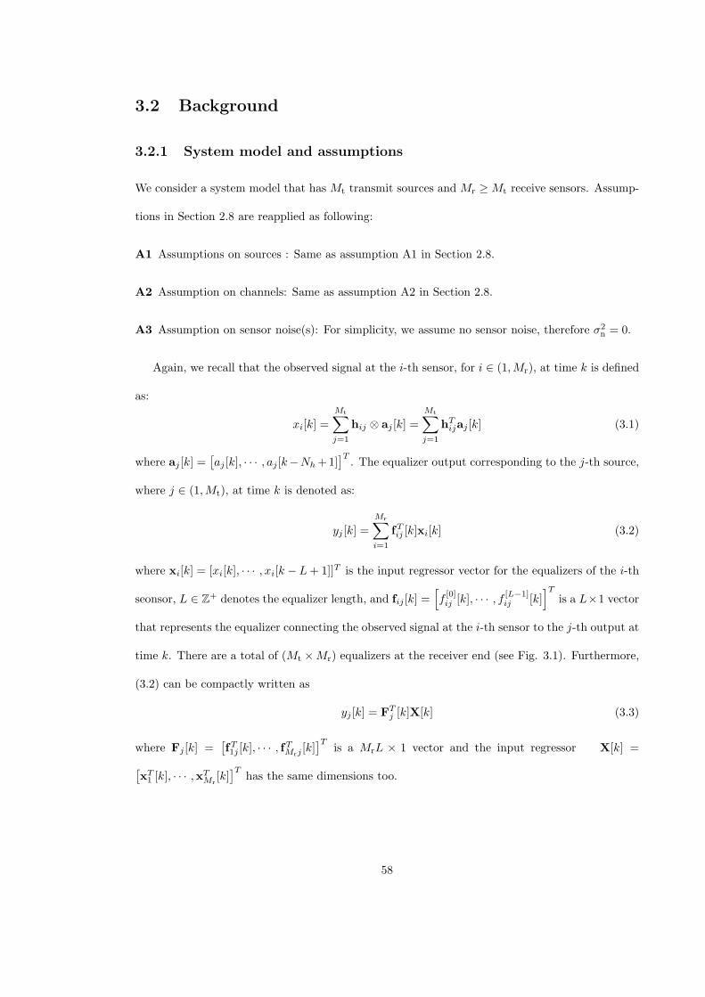
3.2 Background
3.2.1 System model and assumptions
We consider a system model that has Mt transmit sources and Mr ≥Mt receive sensors. Assump-
tions in Section 2.8 are reapplied as following:
A1 Assumptions on sources : Same as assumption A1 in Section 2.8.
A2 Assumption on channels: Same as assumption A2 in Section 2.8.
A3 Assumption on sensor noise(s): For simplicity, we assume no sensor noise, therefore σ2n = 0.
Again, we recall that the observed signal at the i-th sensor, for i ∈ (1,Mr), at time k is defined
as:
xi[k] =
Mt∑j=1
hij ⊗ aj [k] =
Mt∑j=1
hTijaj [k] (3.1)
where aj [k] =[aj [k], · · · , aj [k−Nh+1]
]T. The equalizer output corresponding to the j-th source,
where j ∈ (1,Mt), at time k is denoted as:
yj [k] =
Mr∑i=1
fTij [k]xi[k] (3.2)
where xi[k] = [xi[k], · · · , xi[k − L+ 1]]T is the input regressor vector for the equalizers of the i-th
seonsor, L ∈ Z+ denotes the equalizer length, and fij [k] =[f[0]ij [k], · · · , f [L−1]
ij [k]]T
is a L×1 vector
that represents the equalizer connecting the observed signal at the i-th sensor to the j-th output at
time k. There are a total of (Mt ×Mr) equalizers at the receiver end (see Fig. 3.1). Furthermore,
(3.2) can be compactly written as
yj [k] = FTj [k]X[k] (3.3)
where Fj [k] =[fT1j [k], · · · , fTMrj
[k]]T
is a MrL × 1 vector and the input regressor X[k] =[xT1 [k], · · · ,xT
Mr[k]]T
has the same dimensions too.
58
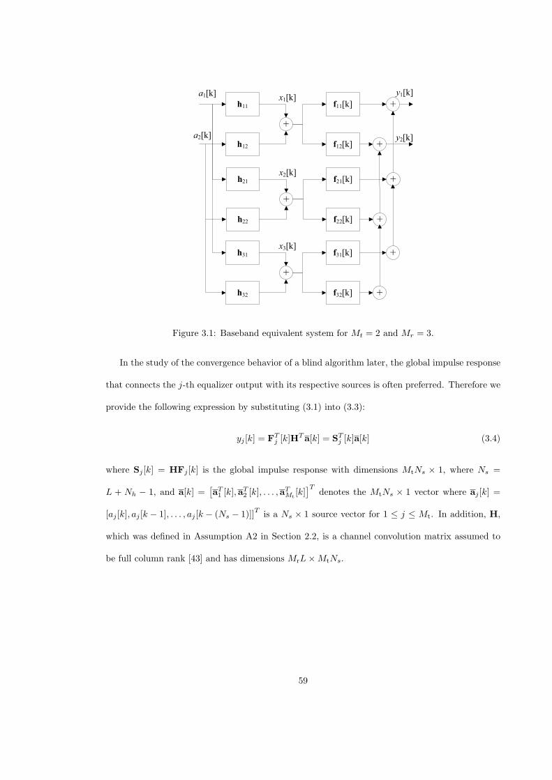
h11
a1[k]
f11[k]
+
h12 f12[k]
+
+a2[k]
x1[k]y1[k]
y2[k]
h21 f21[k]
+
h22 f22[k]
+
+
x2[k]
h31 f31[k]
+
h32 f32[k]
+
+
x3[k]
Figure 3.1: Baseband equivalent system for Mt = 2 and Mr = 3.
In the study of the convergence behavior of a blind algorithm later, the global impulse response
that connects the j-th equalizer output with its respective sources is often preferred. Therefore we
provide the following expression by substituting (3.1) into (3.3):
yj [k] = FTj [k]H
Ta[k] = STj [k]a[k] (3.4)
where Sj [k] = HFj [k] is the global impulse response with dimensions MtNs × 1, where Ns =
L + Nh − 1, and a[k] =[aT1 [k],a
T2 [k], . . . ,a
TMt
[k]]T
denotes the MtNs × 1 vector where aj [k] =
[aj [k], aj [k − 1], . . . , aj [k − (Ns − 1)]]Tis a Ns × 1 source vector for 1 ≤ j ≤ Mt. In addition, H,
which was defined in Assumption A2 in Section 2.2, is a channel convolution matrix assumed to
be full column rank [43] and has dimensions MrL×MtNs.
59
3.2.2 Classical mixed cost approach
A classical approach to perform blind signal separation (BSS) of a linear convolutive mixture of
signals is to combine the costs of the CMA, Jj,CM(F), and a source separation cost function,
Jj,SS(F). Therefore the mixed cost function responsible for the extraction of the j-th source is
Jj,SS−CMA(F) = Jj,CMA(F) + 2kjJj,SS(F) (3.5)
where kj is known as the mixing parameter that corresponds to the equalizer output j and k1 = 0
was suggested to reduce the computation complexity [2]. The CMA opens the channel eye by
minimizing the following cost [36]:
Jj,CM(F) = E(|yj |2 − Rj
)2(3.6)
where Rj = m4/σ2A is known as the dispersion constant [21], whereas the BSS algorithm minimizes
this cost:
Jj,SS(F) =
j−1∑n=1
δx∑δ=−δx
ζn,δ (3.7)
where ζn,δ is a function of the j-th output and the n-th output which is delayed by −δx ≤ δ ≤ δx
symbols relative to the j-th output, where δx ∈ Z+ ≥ Ns − 1 is the maximum achievable delay
between all equalized outputs. This function is responsible for blind source separation and may
take the form of the following cross-correlation (CC) function [2, 31, 42, 43, 44, 45, 46],
ζn,δ , ζCC,n,δ = |Eyj [k]y∗n[k − δ]|2 . (3.8)
For practical implementation under stochastic gradient adaptation, the coefficients of the j-th
equalizer are updated as follows:
Fj [k + 1] = Fj [k]− µj∂Jj,SS−CMA(F)
∂Fj [k](3.9)
= Fj [k]− µj emix,j [k] X∗[k] (3.10)
where µj is a small step size associated with the j-th equalizer and, with Eq. 3.5, the general
60
gradient,∂Jj,SS−CMA(F)
∂Fj [k]is
∂Jj,SS−CMA(F)
∂Fj [k]≡ ∂Jj,CM(F)
∂Fj [k]+ kj
∂Jj,SS(F)
∂Fj [k](3.11)
= (εj,CM,j [k] + kjεj,SS[k])X∗[k] = emix,j [k]X
∗[k]. (3.12)
where εj,CM,j [k], εj,SS,j [k] and emix,j [k] = εj,CM[k] + kjεj,SS[k] are known as the CMA error, the
source separation error and the mixed error respectively for the j-th equalizer.
3.2.3 Motivation: shrinking of the equalizer output
We now highlight an implementation difficulty associated with the traditional mixed cost method,
which arises due to the source separation cost, Eq. (3.7). Consider the CC function in Eq (3.8). It
is a square-modulus function of an expectation function in the form of |E(·)|2 whereas conventional
costs are regular expectation functions, E(·), which gives an unbiased estimate when instantaneous
values are taken. With the modulus function, the expectation function within it cannot be simply
omitted without incurring a bias in the estimator. A commonly adopted approach is to explicitly
estimate∂JSS,j(F)∂Fj [k]
based on instantaneous values or sample averaging [31]. In symbol-rate imple-
mentations, for example, a recursive estimator can be used to perform sample averaging as follows
[46]
rn,δ[k] = λrn,δ[k − 1] + (1− λ)yj [k]y∗n[k − δ] (3.13)
and λ ∈ (0, 1] is a forgetting factor. When λ = 0, the process becomes estimation by taking
instantaneous values. The impact of using the above recursive estimator has not been studied
before, and it is the purpose of this subsection.
Proposition: This estimator will introduce an undesirable bias that amounts to (j − 1)(2δx +
1)σ4A(1− λ)/(1 + λ).
61
Proof: We determine the bias by evaluating the mean of the estimate as follows:
E|rn,δ[k]|2
= E∣∣λrn,δ[k − 1] + (1− λ)yj [k]y
∗n[k − δ]
∣∣2 (3.14)
= E∣∣(1− λ)Σ∞
d=0λdyj [k − d]y∗n[k − δ − d]
∣∣2 (3.15)
= (1− λ)2∞∑d=0
λ2dE∣∣aj [k − d]
∣∣2E∣∣an[k − δ − d]∣∣2 (3.16)
= (σ2A)
2(1− λ)2Σ∞d=0λ
2d (3.17)
= σ4A(1− λ)/(1 + λ) > 0. (3.18)
The important manipulations of Equations 3.14–3.18 are stated as below.
• From Eq. 3.14 to Eq. 3.15: Using Eq. 3.13, we evaluate all past CC estimates 1, i.e.,
λrn,δ[k − 1], λrn,δ[k − 2],..., λrn,δ[k −∞] and then recursively substituting them back until
we get λrn,δ[k − 1] and therefore we get Eq. 3.15.
• From Eq. 3.15 to Eq. 3.16: The largest concern of this portion is how to mathematically
describe the equalizer outputs (yj [k] and yn[k]) in term of the source symbols (aj [k] and
an[k]). In the asymptotic condition or the steady state (i.e. time k → ∞), the source
symbols are assumed to be perfectly recovered and separated without any interference in Eq.
3.4 (where this is a common assumption to verify a bias [113]), thus we have yj [k] → aj [k]
and yn[k] → an[k]. In addition, an[k] and aj [k] (note: n = j is implicity stated in Eq.3.7) are
mutually independent and discrete time stationary in Assumption A1 (Section 2.8), therefore
E∣∣aj [k− d]
∣∣2∣∣an[k− δ − d]∣∣2 can be simplified as E
∣∣aj [k− d]∣∣2E∣∣an[k− δ − d]
∣∣2. With
the above information, we get Eq. 3.16 after some algebraic manipulations.
• From Eq. 3.16 to Eq. 3.17: We recall Assumption A1 in Section 2.8 that the source symbols
has a common positive variance, σ2A. Therefore, we have σ2
A = E∣∣aj [k − d]
∣∣2 = E∣∣an[k −
δ − d]∣∣2 and we emphasize (σ2
A)2 = σ4
A to avoid confusion.
1For example, to evaluate rn,δ[k − d], we can replace k with k − d in Eq. 3.13, therefore we get rn,δ[k − d] =
λrn,δ[k − 1− d] + (1− λ)yj [k − d]y∗n[k − δ − d].
62
• From Eq. 3.17 to Eq. 3.18: We want to show the equality of Σ∞d=0λ
2d = 1(1−λ)(1+λ) in this
portion. Due to the range of the forgetting factor, λ is given as 0 ≤ λ < 1 in Eq. 3.13, it
is obvious that the range of its square, λ2 is 0 ≤ λ2 < 1. With λ2 < 1, we can simplify the
summation of the infinite geometric series, Σ∞d=0λ
2d = Σ∞d=0(λ
2)d = 1+λ2+λ4+ . . . as 11−λ2 .
Furthermore, we recall a common type of algebraic factoring which is 1 − λ2 = 12 − λ2 =
(1 + λ)(1 − λ), therefore we can factorize the denominator of 11−λ2 and finally we obtain
1(1−λ)(1+λ) .
• Comment on Eq. 3.18: Since λ has the range 0 ≤ λ < 1, the value of Eq. 3.18 is always
larger than zero, therefore the CC estimator, rn,δ[k] is an asymptotic bias estimator even in
the perfect symbol recovery and the perfect source separation conditions. In fact, an unbiased
estimator should give a value of zero in Eq. 3.18. Again, it is worth to mention that the
previous works (such as [2, 31, 42, 43, 44, 45, 46]) had started their developments based on
the assumption that the CC estimator, rn,δ[k] is an unbiased estimator. However, our works
above have proven that the CC estimator, rn,δ[k] is a bias estimator.
The two outer sums in (3.7) introduce the factor (j−1)(2δx+1) to the total bias, which completes
the proof.
This finite bias is the reason behind the equalizer output shrinking in magnitude, a behaviour
that can be explained using our extrema (stationary point) analysis in Section 3.3.4. The shrinking
effect is further accentuated with increased number of users and delay spread, hence restricting
the usefulness of the algorithm to MIMO systems with few users and/or small delay spread, for
example in polarized optical receivers where only two orthogonal polarizations (users) exist [46].
63
3.3 New Cross Independent Constant Modulus Algorithm
(CI-CMA)
3.3.1 A new BSS cost: the cross independent function
Our intention is to propose a new BSS cost that is conventional in the sense that it conforms to
E(·). Therefore we propose the so-called “cross-independent” (CI) function
ζCI,n,δ = E|yjy∗n,δ|2
(3.19)
where its derivative w.r.t. Fj [k] is
∂
∂Fj [k]ζCI,n,δ = yj [k]y
∗n[k − δ]yn[k − δ]X∗[k]. (3.20)
The minimization of the CI cost leads to a stronger independence property (than decorrelation)
among the equalizer outputs whose proof is documented in Appendix A.1 (at the end of this thesis).
Therefore the complete algorithm for blind equalization and source separation is the combination
of the MIMO CMA and this CI cost, called the CI-CMA, which has the following cost function,
Jj,CI−CMA(F) = Jj,CMA(F) + k0
j−1∑n=1
δx∑δ=−δx
ζCI,n,δ (3.21)
and the corresponds error term is
emix,j [k] =(|yj [k]|2 − Rj
)yj [k] +
k02
j−1∑n=1
δx∑δ=−δx
(|yn[k − δ]|2
)yj [k]. (3.22)
where k0 is the new mixing parameter of the CI cost and its value will be determined later. We
would like to draw the attention of the reader to the dispersion constant of the CMA, Rj , which
has been modified to ensure the original signal energy is preserved at its corresponding equalizer
output. It will be proven in the sequel that the new value of Rj solves the output-shrinking problem
encountered by past approaches. Under the hierarchical criteria [2], we have R1 < R2 < · · · < RMt ,
and R1 = m4
σ2A
because for j = 1 the CI-CMA reduces to the classical MIMO CMA without the
BSS cost. For completeness, we state the value of Rj under the symmetrical criteria [31] to be
64
R1 = R2 = · · · = RMt but Rj = m4
σ2A, ∀j. The expression of the dispersion constant is left as the
subject of the next subsection when the stationary points of the cost surface are derived.
In what follows, we first search for the global minimum points of the CI-CMA under gradient
descent adaptation. We subsequently determine the conditions for which all spurious local minima
of the CI-CMA would vanish, so that the global minima is always achieved. A real-valued PAM
system is assumed here whereas the treatment of the complex modulation is found in Section 3.4.
3.3.2 Preliminary assumptions and useful notations
For simplicity but without losing generality, we confine our analysis to a Mt = 2 MIMO system.
Therefore for j = 1 the MIMO CMA extracts any source, but usually the one that enjoys a stronger
SNR, while for j = 2 the equalizer must avoid the retrieval of the same source thanks to the CI
cost.
For convenience, the global impulse response of the second equalizer is expressed as a concate-
nation of two vectors, i.e., S2 = [ST(1),2,S
T(2),2]
T which is MtNs = 2Ns long (see Eq (3.4)), where
S(b),2 = [S[(b−1)Ns]2 , S
[(b−1)Ns+1]2 , · · · , S[bNs−1]
2 ]T is the global filter vector that connects the b-th
source to the second equalizer. The time dependency of S2 on k is dropped because the analysis
is based on asymptotic conditions. The global impulse response of the first equalizer, which will
be required later, are also expressed as vectors α , S(1),1 and β , S(2),1 connecting the first and
second sources, respectively, to the output of the first equalizer, i.e., S1 ,[αT , βT
]T. The use of
new variables α and β is to conveniently distinguish S1 from S2. Their respective i-th elements
are αi = S[i]1 and βi = S
[Ns+i]1 , where i ∈ (0, Ns − 1).
We further assume that in analyzing the j-th equalizer that the previous (j − 1) equalizers up
in the hierarchy have been perfectly equalized. In our Mt = 2 case, we assume the first equalizer
has perfectly recovered one of the sources (usually the stronger one) and thus Eαi|i =d = 0 where
the only non-zero impulse is at the (d+ 1)-th tap, where d ∈ (0, Ns − 1). In fact Eαd = 1. We
assume that it has also canceled all CCI so Eβi = 0, ∀i. To be more practical, we further assume
65
the variance of the non-dominant taps are finite, i.e., Σi =dE|αi|2
> 0 and ΣjE
|βj |2
> 0. Due
to the unity-impulse in αd, we have the relationship of E∥α∥2 > E∥β∥2 where ∥ · ∥ is the Euclidean
norm operator.
3.3.3 Extrema analysis
We now begin the stationary point analysis. For brevity, we denote J2[k] , Jmix,2(F). We evaluate
the gradient of J2[k] w.r.t. S2 in the following equations from (3.25) to (3.33):
∂J2[k]
∂S2=
[(∂J2[k]
∂S(1),2
)T
,
(∂J2[k]
∂S(2),2
)T]T
(3.25)
where
∂J2[k]
∂S(1),2=
[∂J2[k]
∂S[0]2
,∂J2[k]
∂S[1]2
, . . . ,∂J2[k]
∂S[Ns−1]2
]Tand
∂J2[k]
∂S(2),2=
[∂J2[k]
∂S[Ns]2
,∂J2[k]
∂S[Ns+1]2
, . . . ,∂J2[k]
∂S[2Ns−1]2
]T.
We would like to express J2[k] in terms of the global impulse response by using (3.4), so at first
the CM cost is rewritten as
JCM,j = E
(∣∣STj [k]a[k]
∣∣2 − Rj
)2. (3.26)
Bearing in mind that the CI cost in Eq. (3.21) for j = 2 reduces to ΣδζCI,1,δ = ΣδE|y2y∗1,δ|2
=
ΣδEy22y
21,δ
, the mixed-cost becomes
J2[k] = E(
(ST(1),2a1[k] + ST
(2),2a2[k])2 − R2
)2 + k0
δx∑δ=−δx
E
(ST
(1),2a1[k] + ST(2),2a2[k])
2(αTa1[k − δ] + βTa2[k − δ])2.
(3.27)
After significant amount of mathematics, it can be shown that the gradient of the mixed cost is
∂J2[k]
∂S2= 4ΛS2 = 4(ΛCM +ΛCI)S2 (3.28)
66
where Λ is a 2Ns × 2Ns diagonal matrix which can be split into ΛCM and ΛCI, where they are
derived from the CM and CI costs, respectively. To evaluate ΛCM, we evaluate the gradient of
JCM,j w.r.t. S[d0]2 as follows
∂JCM,j
∂S[d0]2
= 4S[d0]2 Λ
[d0]CM (3.29)
where
Λ[d0]CM =
(S[d0]2
)2m4 − 3
(S[d0]2
)2σ4A + 3σ4
A∥S2∥2 − R2σ2A (3.30)
is the d0-th, d0 ∈ (0, 2Ns − 1), diagonal element of ΛCM. As for ΛCI, the mathematics is more
involved. The derivation is recorded in Appendix A.2 (in the end of the thesis) where the d0-th
diagonal element of ΛCI was shown to be
Λ[d0]CI =
k02
((m4 − σ4
A
)E∥∥γ(d0)∥∥2 +Ωo
)(3.31)
where
γ(d0) =
α if d0 ∈ (0, Ns − 1)
β if d0 ∈ (Ns, 2Ns − 1),
(3.32)
∥ · ∥ is the Euclidean norm operator and
Ωo = σ4A (2δx + 1)
(E∥∥α∥∥2 + E
∥∥β∥∥2). (3.33)
At this point, due to the complicated nature of equations (3.29)-(3.33) we categorize the sta-
tionary points (where Eq. 3.28 equals to zero) under the following four cases where they could be
found:
Case 1: S[d0]2 = 0, for all d0 ∈ (0, 2Ns − 1). This undesirable case implies a zero-valued
output at the second equalizer since the global impulse response does not have any non-zero taps.
∴ ∥S2∥2 = 0.
Case 2: S[d0]2 |d0 =b = 0, ∀(d0 = b) where 0 ≤ b ≤ Ns − 1. This undesirable case implies the
successful retrieval of the first source when the intended source is the second. Since only one tap
67
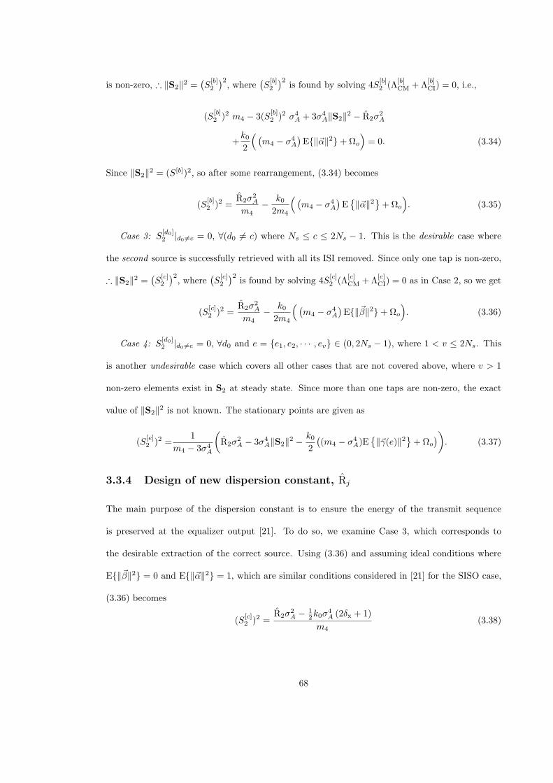
is non-zero, ∴ ∥S2∥2 =(S[b]2
)2, where
(S[b]2
)2is found by solving 4S
[b]2 (Λ
[b]CM + Λ
[b]CI) = 0, i.e.,
(S[b]2 )2 m4 − 3(S
[b]2 )2 σ4
A + 3σ4A∥S2∥2 − R2σ
2A
+k02
( (m4 − σ4
A
)E∥α∥2+Ωo
)= 0. (3.34)
Since ∥S2∥2 = (S[b])2, so after some rearrangement, (3.34) becomes
(S[b]2 )2 =
R2σ2A
m4− k0
2m4
( (m4 − σ4
A
)E∥α∥2
+Ωo
). (3.35)
Case 3: S[d0]2 |d0 =c = 0, ∀(d0 = c) where Ns ≤ c ≤ 2Ns − 1. This is the desirable case where
the second source is successfully retrieved with all its ISI removed. Since only one tap is non-zero,
∴ ∥S2∥2 =(S[c]2
)2, where
(S[c]2
)2is found by solving 4S
[c]2 (Λ
[c]CM +Λ
[c]CI) = 0 as in Case 2, so we get
(S[c]2 )2 =
R2σ2A
m4− k0
2m4
( (m4 − σ4
A
)E∥β∥2+Ωo
). (3.36)
Case 4: S[d0]2 |d0 =e = 0, ∀d0 and e = e1, e2, · · · , ev ∈ (0, 2Ns − 1), where 1 < v ≤ 2Ns. This
is another undesirable case which covers all other cases that are not covered above, where v > 1
non-zero elements exist in S2 at steady state. Since more than one taps are non-zero, the exact
value of ∥S2∥2 is not known. The stationary points are given as
(S[e]2 )2 =
1
m4 − 3σ4A
(R2σ
2A − 3σ4
A∥S2∥2 −k02
((m4 − σ4
A)E∥γ(e)∥2
+Ωo
)). (3.37)
3.3.4 Design of new dispersion constant, Rj
The main purpose of the dispersion constant is to ensure the energy of the transmit sequence
is preserved at the equalizer output [21]. To do so, we examine Case 3, which corresponds to
the desirable extraction of the correct source. Using (3.36) and assuming ideal conditions where
E∥β∥2 = 0 and E∥α∥2 = 1, which are similar conditions considered in [21] for the SISO case,
(3.36) becomes
(S[c]2 )2 =
R2σ2A − 1
2k0σ4A (2δx + 1)
m4(3.38)
68
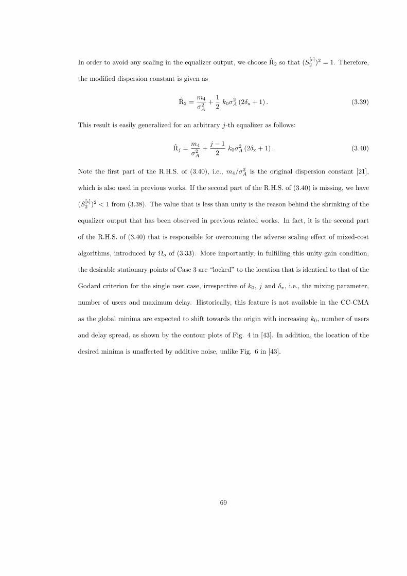
In order to avoid any scaling in the equalizer output, we choose R2 so that (S[c]2 )2 = 1. Therefore,
the modified dispersion constant is given as
R2 =m4
σ2A
+1
2k0σ
2A (2δx + 1) . (3.39)
This result is easily generalized for an arbitrary j-th equalizer as follows:
Rj =m4
σ2A
+j − 1
2k0σ
2A (2δx + 1) . (3.40)
Note the first part of the R.H.S. of (3.40), i.e., m4/σ2A is the original dispersion constant [21],
which is also used in previous works. If the second part of the R.H.S. of (3.40) is missing, we have
(S[c]2 )2 < 1 from (3.38). The value that is less than unity is the reason behind the shrinking of the
equalizer output that has been observed in previous related works. In fact, it is the second part
of the R.H.S. of (3.40) that is responsible for overcoming the adverse scaling effect of mixed-cost
algorithms, introduced by Ωo of (3.33). More importantly, in fulfilling this unity-gain condition,
the desirable stationary points of Case 3 are “locked” to the location that is identical to that of the
Godard criterion for the single user case, irrespective of k0, j and δx, i.e., the mixing parameter,
number of users and maximum delay. Historically, this feature is not available in the CC-CMA
as the global minima are expected to shift towards the origin with increasing k0, number of users
and delay spread, as shown by the contour plots of Fig. 4 in [43]. In addition, the location of the
desired minima is unaffected by additive noise, unlike Fig. 6 in [43].
69
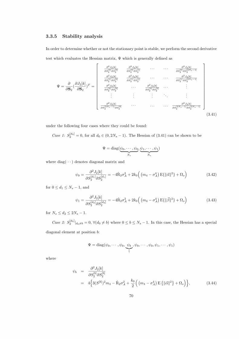
3.3.5 Stability analysis
In order to determine whether or not the stationary point is stable, we perform the second derivative
test which evaluates the Hessian matrix, Ψ which is generally defined as
Ψ =∂
∂S2(∂J2[k]
∂S2)T =
∂2J2[k]
∂S[0]2 ∂S
[0]2
∂2J2[k]
∂S[0]2 ∂S
[1]2
· · · · · · ∂2J2[k]
∂S[0]2 ∂S
[2Ns−1]2
∂2J2[k]
∂S[1]2 ∂S
[0]2
∂2J2[k]
∂S[1]2 ∂S
[1]2
· · · · · · ∂2J2[k]
∂S[1]2 ∂S
[2Ns−1]2
∂2J2[k]
∂S[2]2 ∂S
[0]2
· · · ∂2J2[k]
∂S[3]2 ∂S
[3]2
· · ·...
......
.... . .
...
∂2J2[k]
∂S[2Ns−1]2 ∂S
[0]2
· · · . . . . . . ∂2J2[k]
∂S[2Ns−1]2 ∂S
[2Ns−1]2
(3.41)
under the following four cases where they could be found:
Case 1: S[d0]2 = 0, for all d0 ∈ (0, 2Ns − 1). The Hessian of (3.41) can be shown to be
Ψ = diag(ψ0, · · · , ψ0︸ ︷︷ ︸Ns
, ψ1, · · · , ψ1︸ ︷︷ ︸Ns
)
where diag(· · · ) denotes diagonal matrix and
ψ0 =∂2J2[k]
∂S[d1]2 ∂S
[d1]2
= −4R2σ2A + 2k0
( (m4 − σ4
A
)E∥α∥2+Ωo
)(3.42)
for 0 ≤ d1 ≤ Ns − 1, and
ψ1 =∂2J2[k]
∂S[d2]2 ∂S
[d2]2
= −4R2σ2A + 2k0
( (m4 − σ4
A
)E∥β∥2+Ωo
)(3.43)
for Ns ≤ d2 ≤ 2Ns − 1.
Case 2: S[d0]2 |d0 =b = 0, ∀(d0 = b) where 0 ≤ b ≤ Ns − 1. In this case, the Hessian has a special
diagonal element at position b:
Ψ = diag(ψ0, · · · , ψ0, ψb︸︷︷︸↑
, ψ0, · · · , ψ0, ψ1, · · · , ψ1)
where
ψb =∂2J2[k]
∂S[b]2 ∂S
[b]2
= 43(S[b])2m4 − R2σ
2A +
k02
( (m4 − σ4
A
)E∥α∥2
+Ωo
), (3.44)
70
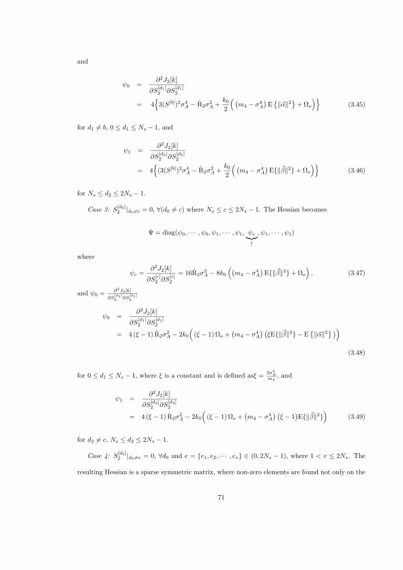
and
ψ0 =∂2J2[k]
∂S[d1]2 ∂S
[d1]2
= 43(S[b])2σ4
A − R2σ2A +
k02
( (m4 − σ4
A
)E∥α∥2
+Ωo
)(3.45)
for d1 = b, 0 ≤ d1 ≤ Ns − 1, and
ψ1 =∂2J2[k]
∂S[d2]2 ∂S
[d2]2
= 4(3(S[b])2σ4
A − R2σ2A +
k02
( (m4 − σ4
A
)E∥β∥2+Ωo
)(3.46)
for Ns ≤ d2 ≤ 2Ns − 1.
Case 3: S[d0]2 |d0 =c = 0, ∀(d0 = c) where Ns ≤ c ≤ 2Ns − 1. The Hessian becomes
Ψ = diag(ψ0, · · · , ψ0, ψ1, · · · , ψ1, ψc︸︷︷︸↑
, ψ1, · · · , ψ1)
where
ψc =∂2J2[k]
∂S[c]2 ∂S
[c]2
= 16R2σ2A − 8k0
((m4 − σ4
A
)E∥β∥2+Ωo
), (3.47)
and ψ0 = ∂2J2[k]
∂S[d1]2 ∂S
[d1]2
ψ0 =∂2J2[k]
∂S[d1]2 ∂S
[d1]2
= 4 (ξ − 1) R2σ2A − 2k0
((ξ − 1)Ωo +
(m4 − σ4
A
) (ξE∥β∥2 − E
∥α∥2
))(3.48)
for 0 ≤ d1 ≤ Ns − 1, where ξ is a constant and is defined asξ =3σ4
A
m4, and
ψ1 =∂2J2[k]
∂S[d2]2 ∂S
[d2]2
= 4 (ξ − 1) R2σ2A − 2k0
((ξ − 1)Ωo +
(m4 − σ4
A
) (ξ − 1
)E∥β∥2
)(3.49)
for d2 = c, Ns ≤ d2 ≤ 2Ns − 1.
Case 4: S[d0]2 |d0 =e = 0, ∀d0 and e = e1, e2, · · · , ev ∈ (0, 2Ns − 1), where 1 < v ≤ 2Ns. The
resulting Hessian is a sparse symmetric matrix, where non-zero elements are found not only on the
71
diagonal but also at the (i, j) and (j, i) positions of the matrix, where i = j and i, j ∈ e. Unlike
cases 1-3, the exact value of ∥S2∥2 is not known here. Using the same approach as in Cases 2 and
3, the stationary point is obtained as
(S[e]2 )2 =
1
m4 − 3σ4A
(R2σ
2A − 3σ4
A∥S2∥2 −k02
((m4 − σ4
A)E∥γ(e)∥2
+Ωo
)). (3.50)
Therefore the Hessian becomes
Ψ = diag(· · · , ψ, ψe1 , ψ, · · · , ψ, ψe2 , ψ, · · · , ψ, ψev , ψ, · · · ) +ev∑
i=e1
ev∑j=e1j =i
Υ(i, j) (3.51)
where Υ(i, j) is a 2Ns × 2Ns square matrix where all its elements are zero except for ∂2J2[k]
∂S[i]2 ∂S
[j]2
at
the i-th row and j-th column. It can be shown that the non-diagonal elements are
∂2J2[k]
∂S[ea]2 ∂S
[eb]2
=∂2J2[k]
∂S[eb]2 ∂S
[ea]2
= 24σ4AS
[ea]2 S
[eb]2 (3.52)
where S[ea]2 and S
[eb]2 are two arbitrary stationary points in e. Therefore the Hessian is non-
diagonal and symmetrical. As for its diagonal elements,
ψe =∂2J2[k]
∂S[e]2 ∂S
[e]2
= 12(S[e]2 )2(m4 − σ4
A) + 12σ4A∥S2∥2 − 4R2σ
2A + 2k0
( (m4 − σ4
A
)E∥γ(e)∥2
+Ωo
)= 8(S
[e]2 )2m4. (3.53)
3.3.6 Design of mixing parameter, k0
The objective of this subsection is to search for and determine a range of values for k0 that admits
the stationary points of Case 3 to be the only ones that are minimum points, while those of Cases
1,2 and 4 are non-minimum. If this is possible, the CI-CMA will become globally convergent to
the desired minima where the desired source is retrieved accurately and without repetition. In this
subsection, we will perform the positive definite test in order to achieve our objective.
Case 1: Referring to equations (3.42) and (3.43), the Hessian matrix is positive definite if and
only if ψ0 > 0 and ψ1 > 0. However since E∥α∥2 > E∥β∥2, we have ψ0 > ψ1 > 0. A necessary
72
and sufficient condition for the stationary point to be unstable is for the opposite to be true, i.e.,
ψ1 ≤ 0. Therefore after substituting R2 of (3.40) into (3.43) we arrive at the inequality (3.54) at
below.
m4
(m4 − σ4A) E∥β∥2+ σ4
A (2δx + 1)(E∥α∥2+ E∥β∥2 − 1
) ≥ k02
(3.54)
Case 2: Referring to equations (3.44), (3.45) and (3.46), it is easy to see that the Hessian
matrix is positive definite if and only if ψb > 0, ψ0 > 0 and ψ1 > 0. Thanks to the assumptions of
m4 ≥ σ4A and E∥α∥2 > E∥β∥2, we have ψb ≥ ψ0 > ψ1 > 0. and it is sufficient to show that
if ψ1 > 0 is true, the Hessian matrix is a positive definite matrix. Since this stationary point is
undesirable, the Hessian should be non-positive definite, i.e., ψ1 ≤ 0. By substituting (3.40) and
(3.35) into (3.46), we arrive at the inequality (3.55), where ξ =3σ4
A
m4.
3σ4A −m4
(m4 − σ4A)(ξE∥α∥2 − E∥β∥2
)+ (ξ − 1)σ4
A (2δx + 1)(E∥α∥2+ E∥β∥2 − 1
) ≤ k02
(3.55)
Case 3: In this desirable case, we wish to find the range of k0 for which the Hessian matrix is
a positive definite matrix. It is necessary and sufficient to satisfy ψc > 0, ψ0 > 0 and ψ1 > 0. Due
the the assumption that E∥α∥2 > E∥β∥2, we have ψ0 > ψ1 > 0. Therefore, we only determine
ψc > 0 and ψ1 > 0. The stationary point has been derived in (3.36). Substituting the expressions
of S[c]2 and R2 from (3.36) and (3.39) into (3.47) and (3.49), we found that both inequalities ψc > 0
and ψ1 > 0 are identical. The resulting inequality is shown in (3.56).
m4
(m4 − σ4A) E∥β∥2+ σ4
A (2δx + 1)(E∥α∥2+ E∥β∥2 − 1
) > k02
(3.56)
Case 4: Since this is an undesirable stationary point we wish to perform the following non-
positive definite test (p. 128 [130]) on the Hessian, so that if the following test fails, it is conclusive
that this stationary point is not a minimum point:(∂2J2[k]
∂S[ea]2 ∂S
[eb]2
)2
<∂2J2[k]
∂S[ea]2 ∂S
[ea]2
· ∂2J2[k]
∂S[eb]2 ∂S
[eb]2
(3.57)
73
Using (3.52) and (3.53), the above test simplifies to 3σ4A < m4, which cannot be true since the
source is circular and sub-Gaussian (see Assumption A1). Therefore the test fails and it is concluded
that the stationary point is unstable.
Finally, the inequalities (3.54), (3.55) and (3.56) are combined to yield the range of k0 values for
which the desired global convergence of the CI-CMA, i.e., blind equalization and source separation
can be achieved:
k0 ≥2m4
(3σ4
A −m4
)3σ4
A (m4 − σ4A)
. (3.58)
Because the denominator is zero when m4 = σ4A, there is no finite value of k0 that can satisfy the
inequality when constant modulus modulation schemes such as the 2-PAM are used.
3.4 Extension to complex modulations
In this section, the results and analysis of Section 3.3 are extended to complex modulations, such
as QAM and PSK. The approach is fairly straight forward with much of its analysis identical to
that of the real-valued case. We must only pay attention to the different statistical properties of
the complex-valued signals, where some values and notations may be different. In particular, we
emphasize that in complex modulations, Ea2j [k] and Ea4j [k] are zero-valued due to the circular
symmetry of the i.i.d. sources, while σ2A = E|aj [k]|2 and m4 = E|aj [k]|4 are the variance and
the fourth order moment of the source, respectively, which have finite positive values in practice.
It can be shown that the gradient of the mixed cost is
∂J2[k]
∂S2= 2ΛS∗
2 = 2(ΛCM +ΛCI)S∗2 (3.59)
where (·)∗ denotes complex conjugate, while Λ, ΛCM and ΛCI are all 2Ns×2Ns diagonal matrices,
and ΛCM can be derived by extending the result of Johnson [121] to complex modulations so that
Λ[d0]CM, the d0-th diagonal element of ΛCM, is expressed as
Λ[d0]CM =
∣∣∣S[d0]2
∣∣∣2m4 − 2∣∣∣S[d0]
2
∣∣∣2 σ4A + 2σ4
A∥S2∥2 − R2σ2A (3.60)
74
where d0 ∈ (0, 2Ns − 1). The d0-th diagonal element of ΛCI is identical to that of the real-valued
case in (3.31)-(3.33).
The Hessian for complex modulations is defined as Ψ = ∂∂S∗
2
(∂J2[k]∂S2
)T, where ∂
∂S∗[i]2
(∂J2[k]
∂S[j]2
)refers to the element in the i-th row and j-th column of Ψ. The subsequent work is identical to
that of the real case, so we simply state the expression of the dispersion constant and the range of
k0 values, derived from the positive definite test which evaluated the Hessian at stationary points
of four cases admitting only the desired solution (Case 3) while discarding the others.
The dispersion constant, Rj , is selected in the same way as (3.40) to avoid undesirable scaling,
with m4 = E|aj [k]|4. As for the mixing parameter, the range of k0 values for which source
separation and equalization can be guaranteed is
k0 ≥m4
(2σ4
A −m4
)σ4A (m4 − σ4
A)(3.61)
where we have assumed E∥α∥2 = 1 and E∥β∥2 = 0. Similar to the real-valued case, no finite
value of k0 can satisfy the inequality when constant modulus modulation schemes such as the
m-ary PSK are used.
75
3.5 Simulations
The simulations are performed in order to identify the open eye and source separation abilities of
the new algorithm CI-CMA for 2-PAM, 4-PAM, 4-QAM and 16-QAM. Furthermore, the shrinking
of equalizer outputs will be identified in the simulations as well.
3.5.1 Simulation Setup
In order to simulate the system model in Section 3.2.1 and Fig. 3.1 with (Mt = 2 and Mr = 3)
MIMO channel, simulations are performed using MATLAB(Matrix Laboratory) version 8.0 . Two
random 2-PAM symbol sequences that have Nseq symbols in one sequence are generated as source
1, a1[k] and source 2, a2[k]. The sources are convoluted with the memory channels hij , and this
process is equivalent to hij ⊗ aj [k] where j = 1, 2. This is aimed to simulate the condition that
the sources are passed through the memory channels and thereby the sources are interfered by
ISI. At the i-th received sensor, the ISI signals from two sources a1[k] and a2[k] (but not a single
source) have been observed, thus the observed signal at i-th sensor xi[k] is corrupted by CCI due
to receiving two sources and ISI due to memory channels. This scenario can be simulated through
computing Eq. 3.1 and the impulse responses of channels hij are stated in Table 3.1.
Next, to simulate the algorithm in the equalizer, we will test using the hierarchical CI-CMA,
i.e., the first equalizer is allowed to recover any of the two sources (usually the stronger one) and
the second equalizer should be able to avoid the extracted source by the first equalizer if BSS works.
The filter weights f11[0] and f22[0] are initialized with a center spike [36] whilst fij [0], ∀i = j, are
initialized with zero-vectors. After the initialization, the observed signals xi[k] are fed through
the filters Fj [k], which is the concatenation vector by several filters fij [k], and generated the two
outputs yj [k] where j = 1, 2 because two sources were transmitted. In this case, this process can be
simulated by executing Eq. 3.3 and the filter values Fj [k] are iteratively updated for every time k
through computing the filter update equation in Eq. 3.10 which has the error term of CI-CMA in
Eq. 3.22. In order to ensure that different sources are not extracted by both equalizers by chance,
76
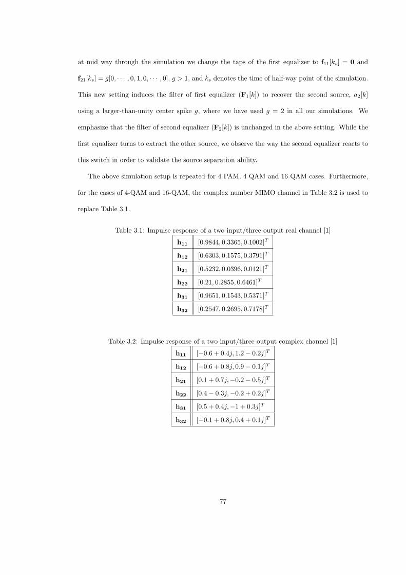
at mid way through the simulation we change the taps of the first equalizer to f11[ks] = 0 and
f21[ks] = g[0, · · · , 0, 1, 0, · · · , 0], g > 1, and ks denotes the time of half-way point of the simulation.
This new setting induces the filter of first equalizer (F1[k]) to recover the second source, a2[k]
using a larger-than-unity center spike g, where we have used g = 2 in all our simulations. We
emphasize that the filter of second equalizer (F2[k]) is unchanged in the above setting. While the
first equalizer turns to extract the other source, we observe the way the second equalizer reacts to
this switch in order to validate the source separation ability.
The above simulation setup is repeated for 4-PAM, 4-QAM and 16-QAM cases. Furthermore,
for the cases of 4-QAM and 16-QAM, the complex number MIMO channel in Table 3.2 is used to
replace Table 3.1.
Table 3.1: Impulse response of a two-input/three-output real channel [1]
h11 [0.9844, 0.3365, 0.1002]T
h12 [0.6303, 0.1575, 0.3791]T
h21 [0.5232, 0.0396, 0.0121]T
h22 [0.21, 0.2855, 0.6461]T
h31 [0.9651, 0.1543, 0.5371]T
h32 [0.2547, 0.2695, 0.7178]T
Table 3.2: Impulse response of a two-input/three-output complex channel [1]
h11 [−0.6 + 0.4j, 1.2− 0.2j]T
h12 [−0.6 + 0.8j, 0.9− 0.1j]T
h21 [0.1 + 0.7j,−0.2− 0.5j]T
h22 [0.4− 0.3j,−0.2 + 0.2j]T
h31 [0.5 + 0.4j,−1 + 0.3j]T
h32 [−0.1 + 0.8j, 0.4 + 0.1j]T
77
3.5.2 Simulation Parameters
In order to perform the simulations, the simulation parameters are required to be defined for the
2-PAM, 4-PAM, 4-QAM and 16-QAM.
First, 2-PAM has the constellation set A = −1, 1 and this constellation set has defined
statistical properties such as fourth order moment m4 = E|a[k]|4
= 1 and variance σ2
A = 1.
In other words, the values of m4 and σ2A are depended on the constellation set A = −1, 1 and
cannot be arbitrary chosen. Next, the step sizes of the equalizers are assigned to be µ1 = 0.001 and
µ2 = 0.0001 for equalizer 1 and 2, respectively. Small value in the step sizes are typically chosen,
but it can cause the convergence becomes slow. On the contrary, large value in the step sizes can
increase the convergence rate but it can cause the equalizer diverges and unstable. Therefore, to
avoid unstable and slow convergence, the above values of step sizes are empirically found after
several simulation attempts had been done. µ2 is smaller than µ1 because the equalizer 2 uses
CI-CMA whilst equalizer 1 uses CMA. Due to CI-CMA can produce larger error than CMA,
µ2 is always chosen to be smaller than µ1 to avoid divergence. The maximum delay is set at
δx = 9 and the lengths of filter are L = 7. Ideally, δx and L that are always larger than the
channel length are theoretically required. However, because we assume the channel is unknown,
therefore, these value are arbitrary chosen. Large values in δx and L is helpful to reduce the
error, but it increases the memory cost. Since L = 7 is chosen, the center tap strategy initializes
f[(L−1)/2]11 [0] = f
[(L−1)/2]22 [0] = 1 and all other taps to zero. Furthermore, based on the analysis
in the previous section, it is clear that no suitable value of k0
2 can satisfy Eq. 3.58 since its
denominator is zero due to m4 = σ4A. Thus we simply choose k0
2 = 2, a value that was suggested
in [2].
Instead of that, the constellation sets A are ±1,±3, ±1 ± j and ±1 ± j,±3 ± j,±1 ±
3j,±3± 3j for 4-PAM, 4-QAM and 16-QAM, respectively. The reasons to select parameters m4,
σ2A, µ1, µ2, δx and L of 4-PAM, 4-QAM and 16-QAM cases are same as the reasons of 2-PAM
case, and the values of the parameters are stated in Table 3.3.
78
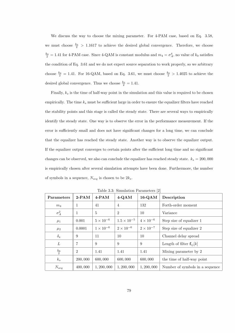
We discuss the way to choose the mixing parameter. For 4-PAM case, based on Eq. 3.58,
we must choose k0
2 > 1.1617 to achieve the desired global convergence. Therefore, we choose
k0
2 = 1.41 for 4-PAM case. Since 4-QAM is constant modulus and m4 = σ4A, no value of k0 satisfies
the condition of Eq. 3.61 and we do not expect source separation to work properly, so we arbitrary
choose k0
2 = 1.41. For 16-QAM, based on Eq. 3.61, we must choose k0
2 > 1.4025 to achieve the
desired global convergence. Thus we choose k0
2 = 1.41.
Finally, ks is the time of half-way point in the simulation and this value is required to be chosen
empirically. The time ks must be sufficient large in order to ensure the equalizer filters have reached
the stability points and this stage is called the steady state. There are several ways to empirically
identify the steady state. One way is to observe the error in the performance measurement. If the
error is sufficiently small and does not have significant changes for a long time, we can conclude
that the equalizer has reached the steady state. Another way is to observe the equalizer output.
If the equalizer output converges to certain points after the sufficient long time and no significant
changes can be observed, we also can conclude the equalizer has reached steady state. ks = 200, 000
is empirically chosen after several simulation attempts have been done. Furthermore, the number
of symbols in a sequence, Nseq is chosen to be 2ks.
Table 3.3: Simulation Parameters [2]
Parameters 2-PAM 4-PAM 4-QAM 16-QAM Description
m4 1 41 4 132 Forth-order moment
σ2A 1 5 2 10 Variance
µ1 0.001 5× 10⁻⁶ 1.5× 10⁻⁵ 4× 10⁻⁶ Step size of equalizer 1
µ2 0.0001 1× 10⁻⁶ 2× 10⁻⁶ 2× 10⁻⁷ Step size of equalizer 2
δx 9 11 10 10 Channel delay spread
L 7 9 9 9 Length of filter fij [k]
k0
2 2 1.41 1.41 1.41 Mixing parameter by 2
ks 200, 000 600, 000 600, 000 600, 000 the time of half-way point
Nseq 400, 000 1, 200, 000 1, 200, 000 1, 200, 000 Number of symbols in a sequence
79
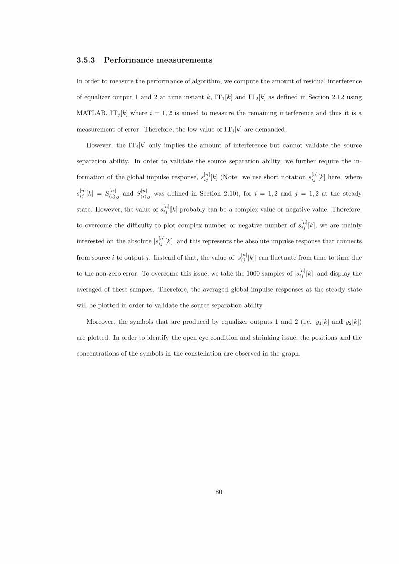
3.5.3 Performance measurements
In order to measure the performance of algorithm, we compute the amount of residual interference
of equalizer output 1 and 2 at time instant k, IT1[k] and IT2[k] as defined in Section 2.12 using
MATLAB. ITj [k] where i = 1, 2 is aimed to measure the remaining interference and thus it is a
measurement of error. Therefore, the low value of ITj [k] are demanded.
However, the ITj [k] only implies the amount of interference but cannot validate the source
separation ability. In order to validate the source separation ability, we further require the in-
formation of the global impulse response, s[n]ij [k] (Note: we use short notation s
[n]ij [k] here, where
s[n]ij [k] = S
[n](i),j and S
[n](i),j was defined in Section 2.10), for i = 1, 2 and j = 1, 2 at the steady
state. However, the value of s[n]ij [k] probably can be a complex value or negative value. Therefore,
to overcome the difficulty to plot complex number or negative number of s[n]ij [k], we are mainly
interested on the absolute |s[n]ij [k]| and this represents the absolute impulse response that connects
from source i to output j. Instead of that, the value of |s[n]ij [k]| can fluctuate from time to time due
to the non-zero error. To overcome this issue, we take the 1000 samples of |s[n]ij [k]| and display the
averaged of these samples. Therefore, the averaged global impulse responses at the steady state
will be plotted in order to validate the source separation ability.
Moreover, the symbols that are produced by equalizer outputs 1 and 2 (i.e. y1[k] and y2[k])
are plotted. In order to identify the open eye condition and shrinking issue, the positions and the
concentrations of the symbols in the constellation are observed in the graph.
80
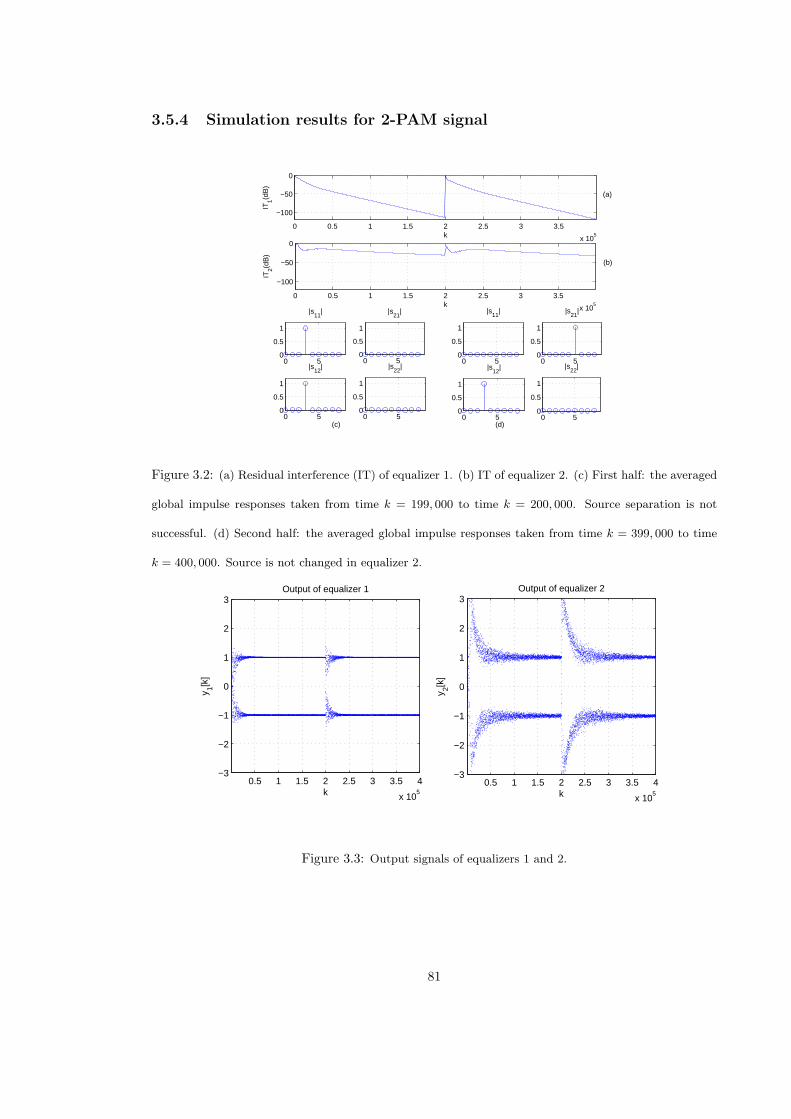
3.5.4 Simulation results for 2-PAM signal
0 0.5 1 1.5 2 2.5 3 3.5
x 105
−100
−50
0
IT1(d
B)
k
0 50
0.5
1
|s11
|
0 50
0.5
1
|s21
|
0 50
0.5
1
|s22
|
0 50
0.5
1
|s12
|0 5
0
0.5
1
|s11
|
0 50
0.5
1
|s21
|
0 0.5 1 1.5 2 2.5 3 3.5
x 105
−100
−50
0
IT2(d
B)
k
0 50
0.5
1
|s12
|
0 50
0.5
1
|s22
|
(a)
(b)
(c) (d)
Figure 3.2: (a) Residual interference (IT) of equalizer 1. (b) IT of equalizer 2. (c) First half: the averaged
global impulse responses taken from time k = 199, 000 to time k = 200, 000. Source separation is not
successful. (d) Second half: the averaged global impulse responses taken from time k = 399, 000 to time
k = 400, 000. Source is not changed in equalizer 2.
0.5 1 1.5 2 2.5 3 3.5 4
x 105
−3
−2
−1
0
1
2
3
k
y 1[k]
Output of equalizer 1
0.5 1 1.5 2 2.5 3 3.5 4
x 105
−3
−2
−1
0
1
2
3
k
y 2[k]
Output of equalizer 2
Figure 3.3: Output signals of equalizers 1 and 2.
81
3.5.4.1 Discussions of 2-PAM signal
Fig. 3.2 (a) and (b) illustrate the IT of equalizer 1 and 2 versus time k. In the first half (i.e., from
k = 1 to k = 2×10⁵), the IT values are decreasing as the time k increases. This implies that CMA
and CI-CMA are able to suppress the interferences of equalizer 1 and 2, respectively. Thus, the
equalization task can be achieved.
Next, in order to validate the source separation ability in the first half, we can observe the
averaged global impulse responses in Fig. 3.2 (c). Among the average global impulse responses
|s11|, |s21|, |s12| and |s22|, only |s11| and |s12| present the spikes. The spike in |s11| indicates that
the equalizer 1 recovers source 1, whilst the spike in |s12| implies the equalizer 2 recovers source
1. Therefore, due to equalizers 1 and 2 recover the same source 1, we can ensure that the source
separation ability is failed. This is expected in our analysis because no suitable value of k0
2 can
satisfy Eq. 3.58 due to m4 = σ4A in 2-PAM.
Instead of that, Fig. 3.3 illustrates the outputs of equalizer 1 and 2 versus time k. In the first
half, at the beginning of time where k is near zero, the symbols of output 1 and 2 are scattered
and this implies the outputs are unreliable. As the time k increasing, due to the equalizers have
successfully suppressed the interferences, the outputs converge towards the points 1 and −1, and
this implies the channel eye can be open. Furthermore, the converged points (1 and −1) are same
as the constellation set of 2-PAM, thus we can validate that no shrinking issue has been found.
Again, in the first half of Fig. 3.3, by observing the signals at time k = 0.5×10⁵ to k = 2×10⁵
of equalizer 1 and time k = 1 × 10⁵ to k = 2 × 10⁵ of equalizer 2, the signals do not show any
significant change within these time ranges. Therefore, these time ranges can be defined at the
steady state time ranges of the equalizers. In the steady state, the global impulse responses within
the steady state time ranges are nearly same and only present minor fluctuations. Therefore, we
take the averaged global impulse responses from the time range k = 199, 000 to time k = 200, 000,
which is within the steady state time ranges.
In the second half (i.e., time k = 2× 10⁵ + 1 to time k = 4× 10⁵), during the initial time (i.e.
82
near k = 2× 10⁵ + 1), the IT values in Fig. 3.2 (a) and (b) are high and the signals in Figure 3.3
are scattered. This is because we intentionally change the taps of the first equalizer (as mentioned
in the Simulation Setup) at time k = 2 × 10⁵. In this case, the equalizers require some time to
suppress the interference. By observing Fig. 3.3, we can see that after the time k = 2.5 × 10⁵
of equalizer 1 and the time k = 3 × 10⁵ of equalizer 2, the signals of the equalizers do not show
any significant change. Thus, we can conclude that the equalizers enter the steady state after the
mentioned times. Therefore, we plot the averaged global impulse responses from the time range
k = 399, 000 to time k = 400, 000 in Fig 3.2 (d). Among the four impulse responses, we can see
that |s21| and |s12| have spikes. Therefore, in the second half, the equalizer 1 recovers source 2
and the equalizer 2 recovers source 1. Even though different sources are recovered, the source
separation task is considered failed because the source separation task was failed in the first half
test.
Next, we compare IT of equalizer 1 and 2 in Fig. 3.2 (a) and (b). We can observe that the IT
of equalizer 2, which employs CI-CMA, suffers higher residual interference than IT of equalizer 1,
which uses CMA. This limitation is due to the extra CI term of the CI-CMA.
83
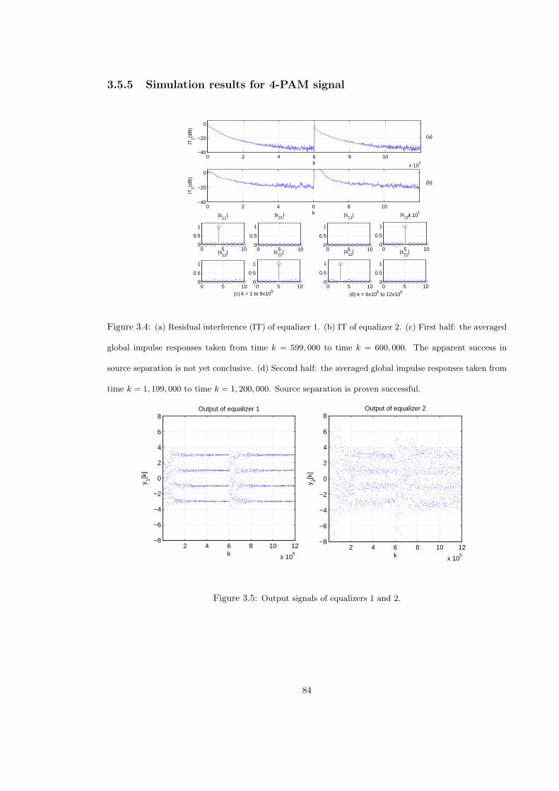
3.5.5 Simulation results for 4-PAM signal
0 2 4 6 8 10
x 105
−40
−20
0
IT1(d
B)
k
0 2 4 6 8 10
x 105
−40
−20
0
IT2(d
B)
k
0 5 100
0.5
1
|s11
|
0 5 100
0.5
1
|s21
|
0 5 100
0.5
1
|s12
|
0 5 100
0.5
1
|s22
| 0 5 100
0.5
1
|s11
|
0 5 100
0.5
1
|s22
|0 5 100
0.5
1
|s21
|
0 5 100
0.5
1
|s12
|
(a)
(b)
(d) k = 6x10⁵ to 12x105(c) k = 1 to 6x10⁵
Figure 3.4: (a) Residual interference (IT) of equalizer 1. (b) IT of equalizer 2. (c) First half: the averaged
global impulse responses taken from time k = 599, 000 to time k = 600, 000. The apparent success in
source separation is not yet conclusive. (d) Second half: the averaged global impulse responses taken from
time k = 1, 199, 000 to time k = 1, 200, 000. Source separation is proven successful.
2 4 6 8 10 12
x 105
−8
−6
−4
−2
0
2
4
6
8
k
y 1[k]
Output of equalizer 1
2 4 6 8 10 12
x 105
−8
−6
−4
−2
0
2
4
6
8
k
y 2[k]
Output of equalizer 2
Figure 3.5: Output signals of equalizers 1 and 2.
84
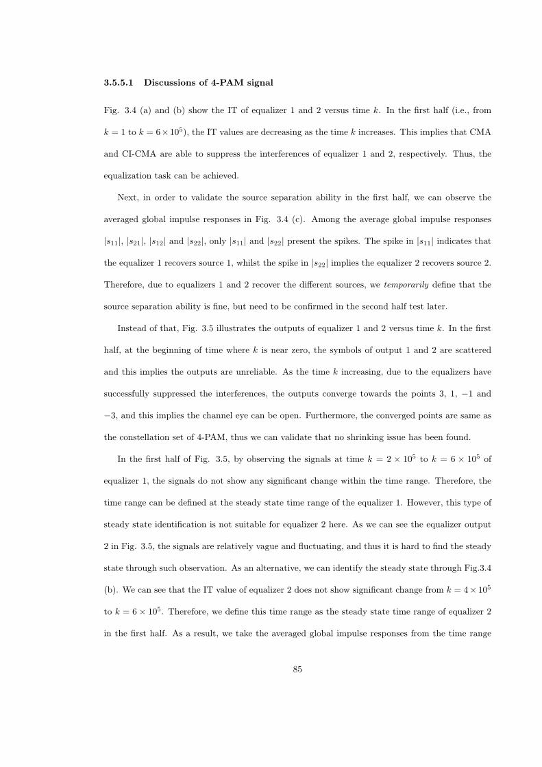
3.5.5.1 Discussions of 4-PAM signal
Fig. 3.4 (a) and (b) show the IT of equalizer 1 and 2 versus time k. In the first half (i.e., from
k = 1 to k = 6×10⁵), the IT values are decreasing as the time k increases. This implies that CMA
and CI-CMA are able to suppress the interferences of equalizer 1 and 2, respectively. Thus, the
equalization task can be achieved.
Next, in order to validate the source separation ability in the first half, we can observe the
averaged global impulse responses in Fig. 3.4 (c). Among the average global impulse responses
|s11|, |s21|, |s12| and |s22|, only |s11| and |s22| present the spikes. The spike in |s11| indicates that
the equalizer 1 recovers source 1, whilst the spike in |s22| implies the equalizer 2 recovers source 2.
Therefore, due to equalizers 1 and 2 recover the different sources, we temporarily define that the
source separation ability is fine, but need to be confirmed in the second half test later.
Instead of that, Fig. 3.5 illustrates the outputs of equalizer 1 and 2 versus time k. In the first
half, at the beginning of time where k is near zero, the symbols of output 1 and 2 are scattered
and this implies the outputs are unreliable. As the time k increasing, due to the equalizers have
successfully suppressed the interferences, the outputs converge towards the points 3, 1, −1 and
−3, and this implies the channel eye can be open. Furthermore, the converged points are same as
the constellation set of 4-PAM, thus we can validate that no shrinking issue has been found.
In the first half of Fig. 3.5, by observing the signals at time k = 2 × 10⁵ to k = 6 × 10⁵ of
equalizer 1, the signals do not show any significant change within the time range. Therefore, the
time range can be defined at the steady state time range of the equalizer 1. However, this type of
steady state identification is not suitable for equalizer 2 here. As we can see the equalizer output
2 in Fig. 3.5, the signals are relatively vague and fluctuating, and thus it is hard to find the steady
state through such observation. As an alternative, we can identify the steady state through Fig.3.4
(b). We can see that the IT value of equalizer 2 does not show significant change from k = 4× 10⁵
to k = 6× 10⁵. Therefore, we define this time range as the steady state time range of equalizer 2
in the first half. As a result, we take the averaged global impulse responses from the time range
85
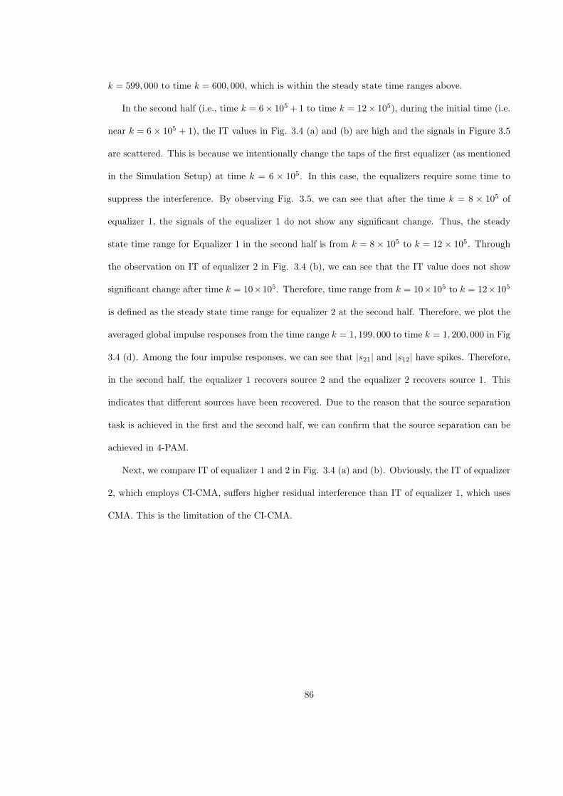
k = 599, 000 to time k = 600, 000, which is within the steady state time ranges above.
In the second half (i.e., time k = 6× 10⁵ +1 to time k = 12× 105), during the initial time (i.e.
near k = 6× 10⁵ + 1), the IT values in Fig. 3.4 (a) and (b) are high and the signals in Figure 3.5
are scattered. This is because we intentionally change the taps of the first equalizer (as mentioned
in the Simulation Setup) at time k = 6 × 10⁵. In this case, the equalizers require some time to
suppress the interference. By observing Fig. 3.5, we can see that after the time k = 8 × 10⁵ of
equalizer 1, the signals of the equalizer 1 do not show any significant change. Thus, the steady
state time range for Equalizer 1 in the second half is from k = 8× 10⁵ to k = 12× 105. Through
the observation on IT of equalizer 2 in Fig. 3.4 (b), we can see that the IT value does not show
significant change after time k = 10×105. Therefore, time range from k = 10×105 to k = 12×105
is defined as the steady state time range for equalizer 2 at the second half. Therefore, we plot the
averaged global impulse responses from the time range k = 1, 199, 000 to time k = 1, 200, 000 in Fig
3.4 (d). Among the four impulse responses, we can see that |s21| and |s12| have spikes. Therefore,
in the second half, the equalizer 1 recovers source 2 and the equalizer 2 recovers source 1. This
indicates that different sources have been recovered. Due to the reason that the source separation
task is achieved in the first and the second half, we can confirm that the source separation can be
achieved in 4-PAM.
Next, we compare IT of equalizer 1 and 2 in Fig. 3.4 (a) and (b). Obviously, the IT of equalizer
2, which employs CI-CMA, suffers higher residual interference than IT of equalizer 1, which uses
CMA. This is the limitation of the CI-CMA.
86
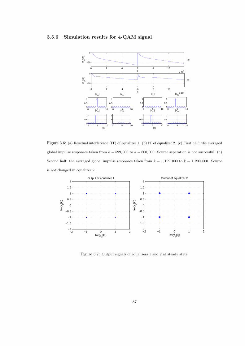
3.5.6 Simulation results for 4-QAM signal
0 2 4 6 8 10
x 105
−50
0
IT1(d
B)
k
0 2 4 6 8 10
x 105
−50
0
IT2(d
B)
k
0 5 100
0.5
1
|s11
|
0 5 100
0.5
1
|s21
|
0 5 100
0.5
1
|s12
|
0 5 100
0.5
1
|s22
|0 5 100
0.5
1
|s11
|
0 5 100
0.5
1
|s21
|
0 5 100
0.5
1
|s12
|
0 5 100
0.5
1
|s22
|
(a)
(b)
(c) (d)
Figure 3.6: (a) Residual interference (IT) of equalizer 1. (b) IT of equalizer 2. (c) First half: the averaged
global impulse responses taken from k = 599, 000 to k = 600, 000. Source separation is not successful. (d)
Second half: the averaged global impulse responses taken from k = 1, 199, 000 to k = 1, 200, 000. Source
is not changed in equalizer 2.
−2 −1 0 1 2−2
−1.5
−1
−0.5
0
0.5
1
1.5
2
Im(y
1[k])
Re(y1[k])
Output of equalizer 1
−2 −1 0 1 2−2
−1.5
−1
−0.5
0
0.5
1
1.5
2
Im(y
2[k])
Re(y2[k])
Output of equalizer 2
Figure 3.7: Output signals of equalizers 1 and 2 at steady state.
87
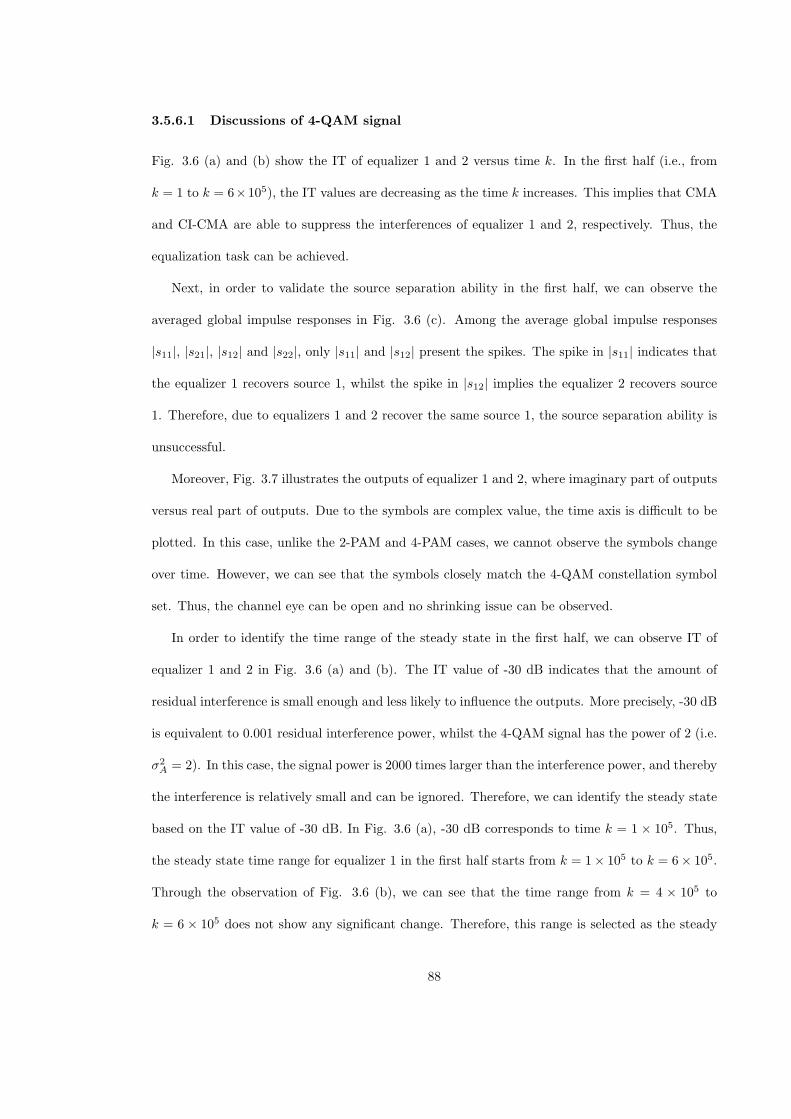
3.5.6.1 Discussions of 4-QAM signal
Fig. 3.6 (a) and (b) show the IT of equalizer 1 and 2 versus time k. In the first half (i.e., from
k = 1 to k = 6×10⁵), the IT values are decreasing as the time k increases. This implies that CMA
and CI-CMA are able to suppress the interferences of equalizer 1 and 2, respectively. Thus, the
equalization task can be achieved.
Next, in order to validate the source separation ability in the first half, we can observe the
averaged global impulse responses in Fig. 3.6 (c). Among the average global impulse responses
|s11|, |s21|, |s12| and |s22|, only |s11| and |s12| present the spikes. The spike in |s11| indicates that
the equalizer 1 recovers source 1, whilst the spike in |s12| implies the equalizer 2 recovers source
1. Therefore, due to equalizers 1 and 2 recover the same source 1, the source separation ability is
unsuccessful.
Moreover, Fig. 3.7 illustrates the outputs of equalizer 1 and 2, where imaginary part of outputs
versus real part of outputs. Due to the symbols are complex value, the time axis is difficult to be
plotted. In this case, unlike the 2-PAM and 4-PAM cases, we cannot observe the symbols change
over time. However, we can see that the symbols closely match the 4-QAM constellation symbol
set. Thus, the channel eye can be open and no shrinking issue can be observed.
In order to identify the time range of the steady state in the first half, we can observe IT of
equalizer 1 and 2 in Fig. 3.6 (a) and (b). The IT value of -30 dB indicates that the amount of
residual interference is small enough and less likely to influence the outputs. More precisely, -30 dB
is equivalent to 0.001 residual interference power, whilst the 4-QAM signal has the power of 2 (i.e.
σ2A = 2). In this case, the signal power is 2000 times larger than the interference power, and thereby
the interference is relatively small and can be ignored. Therefore, we can identify the steady state
based on the IT value of -30 dB. In Fig. 3.6 (a), -30 dB corresponds to time k = 1 × 10⁵. Thus,
the steady state time range for equalizer 1 in the first half starts from k = 1× 10⁵ to k = 6× 10⁵.
Through the observation of Fig. 3.6 (b), we can see that the time range from k = 4 × 10⁵ to
k = 6 × 10⁵ does not show any significant change. Therefore, this range is selected as the steady
88
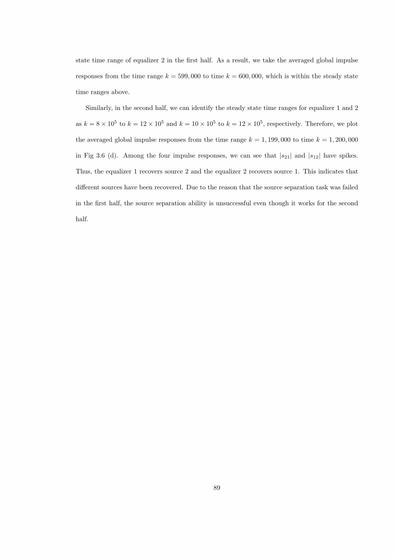
state time range of equalizer 2 in the first half. As a result, we take the averaged global impulse
responses from the time range k = 599, 000 to time k = 600, 000, which is within the steady state
time ranges above.
Similarly, in the second half, we can identify the steady state time ranges for equalizer 1 and 2
as k = 8× 10⁵ to k = 12× 105 and k = 10× 105 to k = 12× 105, respectively. Therefore, we plot
the averaged global impulse responses from the time range k = 1, 199, 000 to time k = 1, 200, 000
in Fig 3.6 (d). Among the four impulse responses, we can see that |s21| and |s12| have spikes.
Thus, the equalizer 1 recovers source 2 and the equalizer 2 recovers source 1. This indicates that
different sources have been recovered. Due to the reason that the source separation task was failed
in the first half, the source separation ability is unsuccessful even though it works for the second
half.
89
3.5.7 Simulation results for 16-QAM signal
0 5 100
0.5
1
|s11
|
0 5 100
0.5
1
|s21
|
0 5 100
0.5
1
|s22
|0 5 100
0.5
1
|s11
|
0 5 100
0.5
1
|s21
|
0 5 100
0.5
1
|s22
|
0 5 100
0.5
1
|s12
|
0 2 4 6 8 10
x 105
−30
−20
−10
0
IT1(d
B)
k
0 2 4 6 8 10
x 105
−30
−20
−10
0
IT2(d
B)
k
0 5 100
0.5
1
|s12
|
(a)
(b)
(c) (d)
Figure 3.8: (a) Residual interference (IT) of equalizer 1. (b) IT of equalizer 2. (c) First half: the
averaged global impulse responses taken from k = 599, 000 to k = 600, 000. The apparent success in
source separation is not yet conclusive. (d) Second half: the averaged global impulse responses taken from
k = 1, 199, 000 to k = 1, 200, 000. Source separation is proven successful.
−4 −2 0 2 4−4
−3
−2
−1
0
1
2
3
4
Re(y1[k])
Im(y
1[k])
Output of equalizer 1
−4 −2 0 2 4−4
−3
−2
−1
0
1
2
3
4
Re(y2[k])
Im(y
2[k])
Output of equalizer 2
Figure 3.9: Output signals of equalizers 1 and 2 at steady state.
90
3.5.7.1 Discussions of 16-QAM signal
Fig. 3.8 (a) and (b) show the IT of equalizer 1 and 2 versus time k. In the first half (i.e., from
k = 1 to k = 6×10⁵), the IT values are decreasing as the time k increases. This implies that CMA
and CI-CMA are able to suppress the interferences of equalizer 1 and 2, respectively. Thus, the
equalization task can be achieved.
Next, in order to validate the source separation ability in the first half, we can observe the
averaged global impulse responses in Fig. 3.8 (c). Among the average global impulse responses
|s11|, |s21|, |s12| and |s22|, only |s11| and |s22| present the spikes. The spike in |s11| indicates that
the equalizer 1 recovers source 1, whilst the spike in |s22| implies the equalizer 2 recovers source 1.
Therefore, due to equalizers 1 and 2 recover the different sources, the source separation ability is
temporarily successfully.
Moreover, Fig. 3.9 illustrates the outputs of equalizer 1 and 2, where imaginary part of outputs
versus real part of outputs. Due to the symbols are complex value, the time axis is difficult to be
plotted. In this case, unlike the 2-PAM and 4-PAM cases, we cannot observe the symbols change
over time. However, we can see that the symbols closely match the 16-QAM constellation symbol
set. Thus, the channel eye can be open and no shrinking issue can be observed.
In order to identify the time range of the steady state in the first half, we can observe IT of
equalizer 1 and 2 in Fig. 3.8 (a) and (b). The time ranges from k = 0.5× 10⁵ to k = 6× 10⁵ and
from k = 4× 10⁵ to k = 6× 10⁵ are chosen to be the steady state time ranges for output 1 and 2,
respectively, because no significant change in IT values can be observed within these time ranges.
As a result, we take the averaged global impulse responses from the time range k = 599, 000 to
time k = 600, 000, which is within the steady state time ranges above.
Similarly, in the second half, we can identify the steady state time ranges for equalizer 1 and 2
as k = 6.5× 10⁵ to k = 12× 105 and k = 10× 105 to k = 12× 105, respectively. Therefore, we plot
the averaged global impulse responses from the time range k = 1, 199, 000 to time k = 1, 200, 000
in Fig 3.8 (d). Among the four impulse responses, we can see that |s21| and |s12| have spikes.
91
Thus, the equalizer 1 recovers source 2 and the equalizer 2 recovers source 1. This indicates that
different sources have been recovered. Since the source separation ability can be found in the first
and the second half, we conclude that the source separation ability can be achieved in 16-QAM.
3.5.8 Summary
We have presented the simulation results for CI-CMA on 2-PAM, 4-PAM, 4-QAM and 16-QAM.
CI-CMA can open the channel eye and does not introduce any shrinking issue on the 4 cases.
For the multi-modulus modulation schemes such as 4-PAM and 16-QAM, CI-CMA can perform
equalization and source separation ability simultaneously. However, CI-CMA is not able to perform
the source separation task in the single-modulus modulation schemes such as 2-PAM and 4-QAM.
92
Chapter 4
Steady State MSE Analysis of the
CI-CMA
4.1 Introduction
We have developed a new MIMO algorithm, CI-CMA in the previous chapter. Indeed, we have
shown its convergence analysis and source separation ability. It is also important to evaluate the
steady steady MSE of the algorithm because this is often used as a performance measurement for
equalization algorithm. Therefore, the chief purpose of this chapter is to perform an accurate steady
state MSE analysis for the CI-CMA using the energy-preserving theorem [54] initially developed for
the single-input/single-output (SISO) blind deconvolutive system. The steady state MSE analysis
has been carried out for the CC-CMA in [50, 131]. In [50], Luo et al have made a good contribution
in analyzing the steady state MSE of the CC-CMA in MIMO systems. Unfortunately, the analysis
in [50, 131] have been done in the presence of the shrinking issue, which results in noticeable
mismatches between the simulation and theoretical results for certain practical range of values.
Therefore, this motivates us to analysis the steady state MSE of the CI-CMA since the shrinking
issue has been resolved in the CI-CMA.
93
We wish to emphasize that the subsequent steady state MSE analysis is carried out with two
major differences than the previous works of [50, 44]. Firstly, we use new dispersion constants,
Rj (shown in the previous chapter) as compared to the conventional dispersion constant, R = m4
σ2A.
Secondly, our MSE analysis is more accurate than [50, 44]. This is because the previous works
analyzed the CC-CMA which is a biased cost function based on energy preservation theorem. It is
worth to mention that the energy preservation theorem was originally established for an unbiased
cost function [54]. Therefore, we improve the previous works by analyzed the new CI-CMA which
is an unbiased cost function based on the energy preservation theorem.
The chapter is organized as follows. Section 4.2 describes the system model and assumptions
made. Section 4.3 briefly describes the generalized CI-CMA. Section 4.4 describes in detail how
the steady state MSE of the CI-CMA is evaluated. Several terms which have previously been
approximated as zero in [50] are re-derived and mathematically proven as finite values that con-
tribute significantly to the steady state MSE. Section 4.5 shows that the MSE obtained through
simulations closely matches the MSE obtained analytically.
4.2 System model and assumptions
We consider the system model that has Mt transmit sources and Mr receive sensors. We further
make the following assumptions:
A1 Assumptions on sources : Same as assumption A1 in Section 2.8. In additional, the signal
has finite positive values on sixth order moment m6 = E|aj [k]|6, fourth order moment
m4 = E|aj [k]|4 and variance σ2A = E|aj [k]|2.
A2 Assumption on channels: Same as assumption A2 in Section 2.2.
A3 Assumption on sensor noise(s): We assume no sensor noise, therefore σ2n = 0.
94
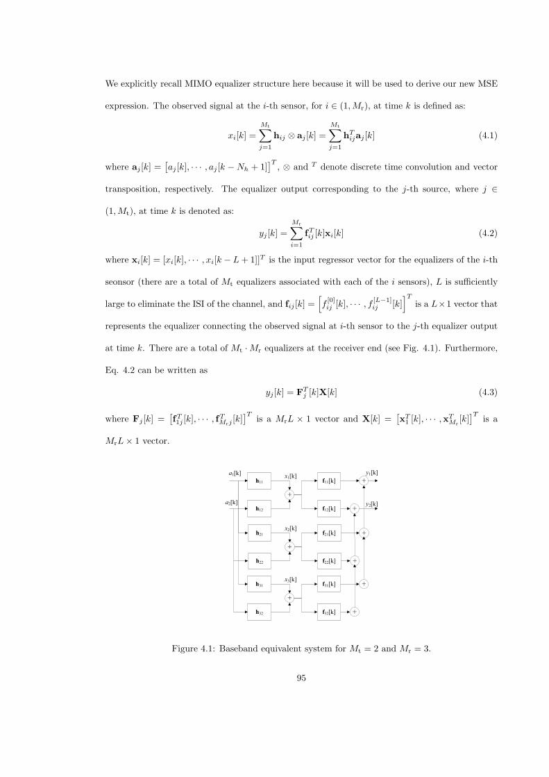
We explicitly recall MIMO equalizer structure here because it will be used to derive our new MSE
expression. The observed signal at the i-th sensor, for i ∈ (1,Mr), at time k is defined as:
xi[k] =
Mt∑j=1
hij ⊗ aj [k] =
Mt∑j=1
hTijaj [k] (4.1)
where aj [k] =[aj [k], · · · , aj [k −Nh + 1]
]T, ⊗ and T denote discrete time convolution and vector
transposition, respectively. The equalizer output corresponding to the j-th source, where j ∈
(1,Mt), at time k is denoted as:
yj [k] =
Mr∑i=1
fTij [k]xi[k] (4.2)
where xi[k] = [xi[k], · · · , xi[k − L+ 1]]T is the input regressor vector for the equalizers of the i-th
seonsor (there are a total of Mt equalizers associated with each of the i sensors), L is sufficiently
large to eliminate the ISI of the channel, and fij [k] =[f[0]ij [k], · · · , f [L−1]
ij [k]]T
is a L×1 vector that
represents the equalizer connecting the observed signal at i-th sensor to the j-th equalizer output
at time k. There are a total of Mt ·Mr equalizers at the receiver end (see Fig. 4.1). Furthermore,
Eq. 4.2 can be written as
yj [k] = FTj [k]X[k] (4.3)
where Fj [k] =[fT1j [k], · · · , fTMrj
[k]]T
is a MrL × 1 vector and X[k] =[xT1 [k], · · · ,xT
Mr[k]]T
is a
MrL× 1 vector.
h11
a1[k]
f11[k]
+
h12 f12[k]
+
+a2[k]
x1[k]y1[k]
y2[k]
h21 f21[k]
+
h22 f22[k]
+
+
x2[k]
h31 f31[k]
+
h32 f32[k]
+
+
x3[k]
Figure 4.1: Baseband equivalent system for Mt = 2 and Mr = 3.
95
4.3 The CI-CMA
The CI-CMA which can mitigate the ISI and CCI simultaneously was proposed in the previous
chapter. In this section, we recall the CI-CMA for Mt sources. For simplicity, we will pursue
Mt = 2. We first state the estimated cost functions and then show its SGA (stochastic gradient
algorithm).
We recall that the cost function of the first equalizer output is the CMA cost function and
the cost function of the jth equalizer output is the CI-CMA cost function. Therefore, the cost
functions of the first and j-th equalizer outputs, J1[k] and Jj [k] are given by
J1[k] = E
(|y1[k]|2 − R1
)2(4.4)
and
Jj [k] = E
(|yj [k]|2 − Rj
)2+ 2kj
Mt∑n=1n =m
δmax∑δ=−δmax
E
∣∣yn[k]y∗m[k − δ]∣∣2 (4.5)
respectively, where R1,Rj ∈ R+ are the dispersion constants where the values will be stated later,
kj ∈ R+ is known as the mixing parameter for the j-th equalizer output and δmax ∈ Z+ accounts
for the maximum channel delay spread between all equalizer outputs.
Now suppose that we wish to extract the j-th source only where j ∈ (1,Mt). By the SGA, the
update equation of the equalizer coefficients, Fj [k], is given as
Fj [k + 1] = Fj [k]− µj (eCMA,j [k] + kjeCI,j [k])X∗[k] (4.6)
where µj is the adaptation step size for the j-th equalizer output, eCMA,j [k] and eCI,j [k] are the
respective error functions of the CMA and cross-independent (CI) terms given as
eCMA,j [k] = (|yj [k]|2 − Rj)yj [k] (4.7)
and
eCI,j [k] =
Mt∑l=1l =j
δmax∑δ=−δmax
yj [k]∣∣yl[k − δ]
∣∣2, (4.8)
96
where yl[k − δ] that involves the past, current or future time l-th equalizer output sample can be
estimated as below [113]
yl[k − δ] = FTl [k]X[k − δ] (4.9)
and
Rj =m4
σ2A
+ βjσ2A (4.10)
is the dispersion constant of the j-th equalizer output with 1
βj = kj(j − 1)(Mt − 1)(2δmax + 1) (4.11)
designed to ensure all the equalizer output energies are restored to the sources’ energies. In
additional, we highlight that the dispersion constant of the first (j = 1) equalizer output, R1 is
m4
σ2A.
4.4 Steady state MSE analysis of CI-CMA
4.4.1 Recap on energy-preserving theorem and assumptions
In order to evaluate the steady state MSE of a blind adaptive equalization algorithm, Mai and
Sayed [54] developed an elegant approach by exploiting the energy-preserving relation of the filter
update process which we now recap. At steady state where we have assumed the equalizer weights
have converged to their global minima, the output of the j-th equalizer will converge towards
yj [k] → aj [k − dj ] exp(jθj)− ea,j [k] (4.12)
where dj is an integer that represents the delay for j-th source and θj is an arbitrary phase offset
which for the purpose of this analysis is assumed θj = 02, and ea,j [k] is due to the gradient noise
1Rj was derived in Section 3.3.4 and the mixing parameter kj is defined as kj = k02
(where k02
was determined
in Section 3.3.6.) in this chapter.2A phase lock loop (PLL) or the multi-modulus algorithm (MMA) may be used to correct the phase offset
experienced by the CMA in the steady state, subject to an arbitrary π/2 offset [132].
97
of the stochastic update algorithm. In fact, the steady state MSE is defined as
MSE = limk→∞
E|ea,j [k]|2
. (4.13)
According to the energy-preserving relation, ea,j [k] is the a-prioiri estimation error and ep,j [k] is
the a-posteriori estimation error, defined as
ea,j [k] = ∆FTj [k]X[k] (4.14)
ep,j [k] = ∆FTj [k + 1]X[k] (4.15)
where ∆Fj [k] = FZF,j − Fj [k] is the difference between the weight vectors of the optimal zero-
forcing (ZF) equalizer and those of the j-th equalizer at time k. Note the ZF equalizer yields
FTZF,jX[k] = aj [k − dj ]exp(jθj).
Mai and Sayed [54] utilized ea,j [k], ep,j [k] and the update equation 4.6 to establish
ep,j [k] = ea,j [k] + µjeo,j [k]∥X[k]∥2 (4.16)
where eo,j [k] = eCMA,j [k]+kjeCI,j [k] accounts for the CI-CMA error function at time k of the j-th
equalizer output. This leads the following energy-preserving relation
E∥∆Fj [k + 1]∥2
+ E
|ea,j [k]|2
∥X[k]∥2
= E
∥∆Fj [k]∥2
+ E
|ep,j [k]|2
∥X[k]∥2
(4.17)
At this point, we state the following assumptions so that the MSE may be extracted from Eq. 4.17
after some mathematical manipulation. At steady state (i.e., k → ∞),
A3 E∥∆Fj [k + 1]∥2
= E
∥∆Fj [k]∥2
, which is a common assumption, c.f. [54, 44, 50, 131];
A4 For a sufficient long equalizer (i.e., L ≫ Nh) and a sufficient small step size (i.e., µj ≈ 0),
∥X[k]∥2 is independent of |eo,j [k]|2 and yj [k] (the details of this assumption can be found in
[54]);
A5 The j-th source, aj [k], is independent with the estimation error at the l-th equalizer output,
ea,l[k], i.e. Eaj [k − dj ]e
∗a,l[k − δ]
= 0 where j ∈ (1,Mr), l ∈ (1,Mr) and dj , δ ∈ Z is an
arbitrary integer, c.f. [50, 131];
98
A6 For L≫ Nh and µj ≈ 0, the estimation error at different equalizer outputs are assumed to be
uncorrelated, i.e. Eea,j [k]e
∗a,l[k − δ]
= 0, c.f. [50] [131];
A7 When µj is small enough, the estimation of Eµj |ea,j [k]|2p
, where p ∈ Z+, is negligible and
can be ignored, c.f. [54, 50].
Equipped with assumptions A3, A4 and Eq. 4.16, we can simplify Eq. 4.17 to
µjE∥X[k]∥2
E|eo,j [k]|2
︸ ︷︷ ︸L.H.S.
= −Eea,j [k]e
∗o,j [k] + e∗a,j [k]eo,j [k]
︸ ︷︷ ︸R.H.S.
(4.18)
The subsequent derivations are aimed at extracting the MSE (c.f. Eq. 4.13) from Eq. 4.18. It is
achieved by systematically expanding the L.H.S. and expressing it in terms of the source statistics,
i.e., E|aj [k]|2
and E
|aj [k]|4
, etc. This manipulation of the L.H.S. is pursued in the next
subsection (Section 4.4.2). After that we expand the R.H.S. and express it in terms of the MSE,
i.e., E|ea,j [k]|2
, and this is done in Section 4.4.3. Finally we equate the L.H.S. and the R.H.S.
to arrive at an expression of the steady state MSE.
4.4.2 Analysis on L.H.S. of Eq. 4.18
The L.H.S. of Eq. 4.18 can be expanded as follows into terms X, A, B, C, and D:
µjE∥X[k]∥2
E|eo,j [k]|2
= µj E
∥X[k]∥2
︸ ︷︷ ︸Term X
(E|eCMA,j [k]|2︸ ︷︷ ︸
Term A
+ k2jE|eCI,j [k]|2︸ ︷︷ ︸Term B
+ kjEe∗CMA,j [k]eCI,j [k]︸ ︷︷ ︸Term C
+ kjEeCMA,j [k]e∗CI,j [k]︸ ︷︷ ︸
Term D
).
(4.19)
4.4.2.1 Term X
Utilizing Assumptions A1, A2 and Eq. 4.1, it can be shown that
E∥X[k]∥2
= Lσ2
A
Mr∑i=1
Mt∑b=1
hHibhib (4.20)
where H denotes Hermitian operator andMr∑i=1
Mt∑b=1
hHibhib denotes the total power gain of the MIMO
channel.
99
4.4.2.2 Term A
Term A, which was derived in [54], is simply
E|eCMA,j [k]|2 = ER2
j |aj [k]|2 − 2Rj |aj [k]|4 + |aj [k]|6. (4.21)
4.4.2.3 Term B
Before we proceed, we wish to highlight that the evaluation of Term B is most different from
previous works [44, 50]. This is because we found that Term B is a function of m4 which had not
been found by the previous works.
By substituting Eq. 4.8 into Term B, we get the following expression
k2jE|eCI,j [k]|2 = k2j
Mt∑n=1n =j
Mt∑l=1l =j
δmax∑δA=−δmax
δmax∑δB=−δmax
gj(n, l, δA, δB) (4.22)
where
gj(n, l, δA, δB) = E|yj [k]|2 |yn[k − δA]|2 |yl[k − δB]|2
. (4.23)
To evaluate Eq. 4.23, we replace yj [k] → aj [kj ] − ea,j [k], where j ∈ (1,Mt) and we abbreviated
kj = k − dj to save space, and then utilizing Assumptions A1, A5, A6 and A7. Then, we get
gj(n, l, δA, δB) ≈ E|aj [kj ]|2
E|an[kn − δA]|2 |al[kl − δB ]|2
. (4.24)
Now, we substitute Eq. 4.24 into Eq. 4.22, we then get the new Term B as
k2jE|eCI,j [k]|2 = k2j
Mt∑n=1n =j
Mt∑l=1l =j
δmax∑δA=−δmax
δmax∑δB=−δmax
E|aj [kj ]|2
E|an[kn − δA]|2 |al[kl − δB ]|2
(4.25)
Regarding to Eq. 4.25, we can identify four scenarios that could occur:
Case 1 : n = l and δA = δB with n = j and l = j;
Case 2 : n = l and δA = δB with n = j and l = j;
Case 3 : n = l and δA = δB with n = j and l = j;
100
Case 4 : n = l and δA = δB with n = j and l = j.
We are going to evaluate the four cases. Among the four cases, Case 1 was not been evaluated in
[50]. In order to obtain an accurate MSE analysis, we determine Case 1 now. In Case 1, we can
evaluate E|aj [kj ]|2E|an[kn − δA]|2|al[kl − δB ]|2 as σ2Am4. In order to complete the evaluation
of Case 1, we wish to know the number of occurrences of Case 1 in Eq. 4.25. Via the summations
Mt∑n=1n=j
Mt∑l=1l =j
δmax∑δA=−δmax
δmax∑δB=−δmax
in Eq. 4.25, we can determine the number of occurrence of Case 1 is
(Mt − 1)(2δmax + 1). Therefore, the final answer of Case 1 is
k2j (Mt − 1)(2δmax + 1)σ2Am4 (4.26)
Next, we evaluate Case 2, 3 and 4 together. In those cases, we notice E|aj [kj ]|2E|an[kn −
δA]|2|al[kl − δB ]|2 = E|aj [kj ]|2E|an[kn − δA]|2E|al[kl − δB ]|2, and therefore we can simplify
it as σ6A. Then, we wish to determine the number of occurrences of those cases. In fact, the number
of occurrences of Case 2, 3 and 4 can be obtained by the number of occurrences of the four cases
subtracts the number of occurrences of Case 1. From Eq. 4.25, the number of occurrences of the
four cases is (Mt − 1)2(2δmax + 1)2, therefore, we can get the number of occurrences of Case 2, 3
and 4 as (Mt − 1)2(2δmax + 1)2 − (Mt − 1)(2δmax + 1). Eventually, we get the combined answer of
Case 2, 3 and 4 which is
k2j((Mt − 1)2(2δmax + 1)2 − (Mt − 1)(2δmax + 1)
)σ6A (4.27)
Finally, combining the answer of Case 1 (Eq. 4.26) and the answer of Case 2, 3 and 4 (Eq.
4.27), we obtain Term B as
k2jE|eCI,j [k]|2 = k2j
((Mt − 1)(2δmax + 1)σ2
Am4 (4.28)
+
((Mt − 1)2(2δmax + 1)2 − (Mt − 1)(2δmax + 1)
)σ6A
)
101
4.4.2.4 Term C & Term D
Terms C and D have identical values as they are complex conjugate of each other. We first consider
Term C in Eq. (4.19). Substituting Eq. 4.7 and Eq. 4.8 into Term C, we then get
kjEe∗CMA,j [k]eCI,j [k] = kj
Mt∑l=1l =j
δmax∑δ=−δmax
E
|yl[k − δ]|2
(|yj [k]|4 − Rj |yj [k]|2
)(4.29)
To evaluate Eq. 4.29, we replace yj [k] → aj [kj ] − ea,j [k], where j ∈ (1,Mt) and we abbreviated
kj = k−dj to save space, then we apply Assumption A7 to ignore small error terms, i.e., E|ea,j [k]|2
and E|ea,j [k]|4. Thus Eq. 4.29 can be simplified as
kjEe∗CMA,j [k]eCI,j [k] = kj(Mt − 1)(2δmax + 1)σ2A
(m4 − Rjσ
2A
). (4.30)
We notice that if Rj is replaced with R = m4
σ2A, then Eq. 4.30 becomes zero. In this case, we
have proven that the approximation of Term C to zero in [50] is valid. The distinction between
our analysis and the previous works of [50, 44] is that we managed to mathematically show that
Term C is actually zero and not merely by assuming it is. However, in this chapter, we consider a
different dispersion constant, i.e., Rj = m4/σ2A + βjσ
2A. Therefore we emphasize that Term C in
Eq. 4.30 is non-zero for the CI-CMA except the first equalizer output (i.e. j = 1). Since Term D
is conjugate counterpart of Term C, the final expression of Term D is same as Eq. 4.30.
4.4.2.5 Combined Expression for L.H.S. of Eq. 4.18
Finally, combining Term X (Eq. 4.20), Term A (Eq. 4.21), Term B (Eq. 4.28), Term C (Eq. 4.30),
Term D (also Eq. 4.30), and replacing Rj with m4/σ2A + βjσ
2A, the L.H.S. of Eq. 4.19 can be
simplified as Eq. 4.31 as below after some algebra manipulations.
µE∥X[k]∥2
E|eo,j [k]|2
︸ ︷︷ ︸L.H.S. of Eq. 4.18
(4.31)
= µLσ2A
( Mr∑i=1
Mt∑b=1
hHibhib
)(m6 −
(m4)2
σ2A
+ kjβjσ2A
(m4 − σ4
A
))
102
4.4.3 Analysis on R.H.S. of Eq. 4.18
The purpose of expanding the R.H.S. of Eq. 4.18 is to find an expression of the MSE, E|ea,j [k]|2,
in a similar fashion as [54, 50, 44]. This can be done by expanding its first term to
Eea,j [k]e
∗o,j [k]
= E
ea,j [k]e
∗CMA,j [k] + kjea,j [k]e
∗CI,j [k]
(4.32)
since e∗o,j [k] = e∗CMA,j [k] + kje∗CI,j [k]. The first term of Eq. 4.32, Eea,j [k]e∗CMA,j [k], has been
derived in [54] before. We simply re-state the result but with a different dispersion constant:
Eea,j [k]e
∗CMA,j [k]
= E|ea,j [k]|2
(Rj − 2σ2
A
). (4.33)
Now we consider the second term in Eq. 4.32. By substituting 4.8 into the term, we get
kjEea,j [k]e
∗CI,j [k]
= kjE
ea,j [k]
Mt∑l=1l =j
δmax∑δ=−δmax
(y∗j [k]|yl[k − δ]|2
)(4.34)
We replace yj [k] → aj [kj ]− ea,j [k] where kj = k − dj for j ∈ (1,Mt) into Eq. 4.34, we then get
kjEea,j [k]e
∗CI,j [k]
(4.35)
= kjE
(a∗j [kj ]ea,j [k]− |ea,j [k]|2
)×( Mt∑
l=1l =j
δmax∑δ=−δmax
(|al[kl − δ]|2 + |ea,l[k]|2 + a∗l [kl − δ]ea,l[k] + al[kl − δ]e∗a,l[k])
))
We apply assumptions A1, A5 and A6 into Eq. 4.35, then Eq. 4.35 can be simplified as
kjEea,j [k]e
∗CI,j [k]
(4.36)
= kjE− |ea,j [k]|2
Mt∑l=1l =j
δmax∑δ=−δmax
(E|al[kl − δ]|2
+ E
|ea,l[k]|2
)
Now, we introduce an assumption from [50] that the error magnitudes are approximately same
which is E|ea,l[k]|2
≈ E
|ea,j [k]|2
. Equipped with the above assumption and the stationary
assumption of the sources in A1, Eq. 4.36 can be further simplified as
−kj(Mt − 1)(δmax + 1)(σ2AE|ea,j [k]|2
+(E|ea,j [k]|2
)2)(4.37)
103
It is not impractical to assume that (E|ea,j [k]|2)2 ≪ E|aj [k]|2E|ea,j [k]|2 (which is the as-
sumption from [50]), and therefore Eq. 4.37 can be further simplified to
kjEea,j [k]e
∗CI,j [k]
≈ −βjσ2
AE|ea,j [k]|2
(4.38)
where βj = kj(Mt − 1)(2δmax + 1) as before, c.f. Eq. 4.11.
After deriving both terms in Eq. 4.32, i.e., Eq. 4.33 and Eq. 4.38, we substitute them back in
Eq. 4.32. By also replacing Rj with m4/σ2A + βjσ
2A, we then get
Eea,j [k]e
∗o,j [k]
= −E
|ea,j [k]|2
(2σ2
A − m4
σ2A
). (4.39)
Now the conjugate counterpart of Eq. 4.32, i.e., Ee∗a,j [k]eo,j [k]
, would have the same expression
as Eq. 4.39. Since both terms are identical, the R.H.S. of Eq. 4.18 is thus
−Eea,j [k]e
∗o,j [k] + e∗a,j [k]eo,j [k]
= 2E
|ea,j [k]|2
(2σ2
A − m4
σ2A
). (4.40)
Note that since Eq. 4.40 has an MSE term in it, our objective to expand the R.H.S. of Eq. 4.18
is achieved.
4.4.4 Expression of the Steady State MSE
Finally, with the L.H.S. of Eq. 4.18 expressed in terms of the source statistics, c.f. (Eq. 4.31),
and the R.H.S. of Eq. 4.18 in terms of the MSE, c.f. (Eq. 4.40), we can proceed to derive an
expression of the steady state MSE of the CI-CMA. By equating the L.H.S. and the R.H.S., the
steady state MSE for the j-th equalizer output can be approximated as Eq. 4.41 which is found
below. We have also intentionally placed the (simplified3) MSE expression derived by Luo et al
[50] in Eq. 4.42 below our MSE expression for the purpose of comparison. For values of kj which
are very close to zero, both Eq. 4.41 and Eq. 4.42 become almost identical. By inspection of Eq.
4.31, it is clear that not only is the steady state MSE being influenced by the statistical properties
of the sources, but it is also influenced by the total power gain of MIMO channels, the selection
3Simplification is achieved by making the assumption of stationarity of the sources.
104
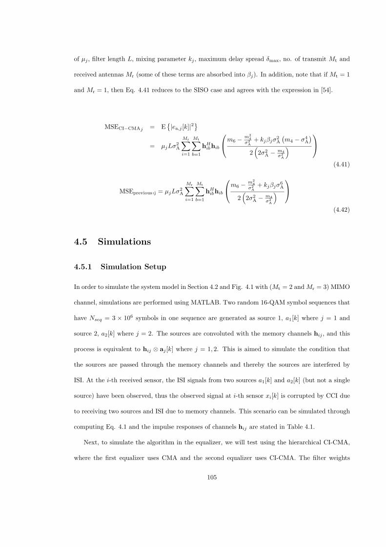
of µj , filter length L, mixing parameter kj , maximum delay spread δmax, no. of transmit Mt and
received antennas Mr (some of these terms are absorbed into βj). In addition, note that if Mt = 1
and Mr = 1, then Eq. 4.41 reduces to the SISO case and agrees with the expression in [54].
MSECI−CMAj = E|ea,j [k]|2
= µjLσ
2A
Mr∑i=1
Mt∑b=1
hHibhib
m6 − m24
σ2A+ kjβjσ
2A
(m4 − σ4
A
)2(2σ2
A − m4
σ2A
)
(4.41)
MSEprevious,j = µjLσ2A
Mr∑i=1
Mt∑b=1
hHibhib
m6 − m24
σ2A+ kjβjσ
6A
2(2σ2
A − m4
σ2A
)
(4.42)
4.5 Simulations
4.5.1 Simulation Setup
In order to simulate the system model in Section 4.2 and Fig. 4.1 with (Mt = 2 andMr = 3) MIMO
channel, simulations are performed using MATLAB. Two random 16-QAM symbol sequences that
have Nseq = 3 × 10⁶ symbols in one sequence are generated as source 1, a1[k] where j = 1 and
source 2, a2[k] where j = 2. The sources are convoluted with the memory channels hij , and this
process is equivalent to hij ⊗ aj [k] where j = 1, 2. This is aimed to simulate the condition that
the sources are passed through the memory channels and thereby the sources are interfered by
ISI. At the i-th received sensor, the ISI signals from two sources a1[k] and a2[k] (but not a single
source) have been observed, thus the observed signal at i-th sensor xi[k] is corrupted by CCI due
to receiving two sources and ISI due to memory channels. This scenario can be simulated through
computing Eq. 4.1 and the impulse responses of channels hij are stated in Table 4.1.
Next, to simulate the algorithm in the equalizer, we will test using the hierarchical CI-CMA,
where the first equalizer uses CMA and the second equalizer uses CI-CMA. The filter weights
105
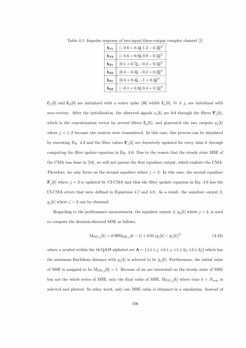
Table 4.1: Impulse response of two-input/three-output complex channel [1]
h11 [−0.6 + 0.4j, 1.2− 0.2j]T
h12 [−0.6 + 0.8j, 0.9− 0.1j]T
h21 [0.1 + 0.7j,−0.2− 0.5j]T
h22 [0.4− 0.3j,−0.2 + 0.2j]T
h31 [0.5 + 0.4j,−1 + 0.3j]T
h32 [−0.1 + 0.8j, 0.4 + 0.1j]T
f11[0] and f22[0] are initialized with a center spike [36] whilst fij [0], ∀i = j, are initialized with
zero-vectors. After the initialization, the observed signals xi[k] are fed through the filters Fj [k],
which is the concatenation vector by several filters fij [k], and generated the two outputs yj [k]
where j = 1, 2 because two sources were transmitted. In this case, this process can be simulated
by executing Eq. 4.3 and the filter values Fj [k] are iteratively updated for every time k through
computing the filter update equation in Eq. 4.6. Due to the reason that the steady state MSE of
the CMA was done in [54], we will not pursue the first equalizer output, which exploits the CMA.
Therefore, we only focus on the second equalizer where j = 2. In this case, the second equalizer
Fj [k] where j = 2 is updated by CI-CMA and thus the filter update equation in Eq. 4.6 has the
CI-CMA errors that were defined in Equations 4.7 and 4.8. As a result, the equalizer output 2,
yj [k] where j = 2 can be obtained.
Regarding to the performance measurement, the equalizer output 2, yj [k] where j = 2, is used
to compute the decision-directed MSE as follows.
MDD,j [k] = 0.99MDD,j [k − 1] + 0.01 |yj [k]− yj [k]|2 (4.43)
where a symbol within the 16-QAM alphabet set A = ±1± j,±3± j,±1±3j,±3±3j which has
the minimum Euclidean distance with yj [k] is selected to be yj [k]. Furthermore, the initial value
of MSE is assigned to be MDD,j [0] = 1. Because of we are interested on the steady state of MSE
but not the whole series of MSE, only the final value of MSE, MDD,j [k] where time k = Nseq, is
selected and plotted. In other word, only one MSE value is obtained in a simulation. Instead of
106
that, the theoretical values that are produced by CI-CMA (i.e. Eq. 4.41) and previous work (i.e.
Eq. 4.42) are plotted
Regarding to the simulation parameters, since 16-QAM alphabet set A = ±1± j,±3± j,±1±
3j,±3 ± 3j is applied, the statistics of this source such as sixth order moment, fourth order
moment and variance have the value of m6 = E|aj [k]|6 = 1960, m4 = E|aj [k]|4 = 132 and
σ2A = E|aj [k]|2 = 10, respectively. Instead of that, the step size of equalizer 1, the length of
channel spread value and the length of filter are assigned to be µ1 = 10−6, δmax = 10 and L = 9.
We are interested to investigate the steady state MSE performance by the various values of
mixing parameter, kj and step size, µj in the equalizer 2, j = 2. Therefore, µj = 1 × 10⁻⁷
and kj = 1.41 are firstly selected and then the simulation is performed as described as in the
first paragraph and eventually a result MSE value is obtained. The simulations are repeated for
kj = 1.46 and kj = 1.51, while the other parameters are unchanged. The MSE results versus the
correspond mixing parameter, kj are plotted as Fig. 4.2.
Next, we set kj = 1.41 and aim to test various values of step size µj in the equalizer 2. The
step sizes values of 0.75× 10⁻⁷, 1× 10⁻⁷, 1.25× 10⁻⁷ and 1.5× 10⁻⁷ are selected. The simulations
are performed and the correspond MSE values are plotted in Fig. 4.3.
107
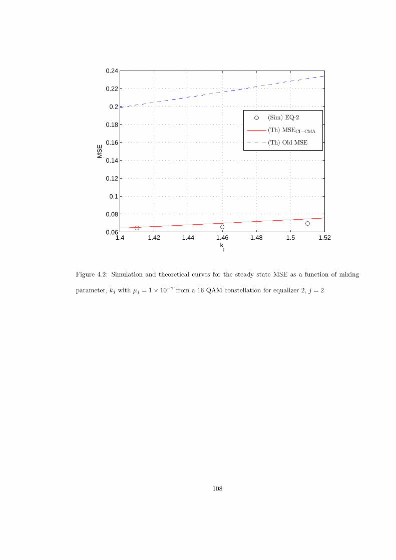
1.4 1.42 1.44 1.46 1.48 1.5 1.520.06
0.08
0.1
0.12
0.14
0.16
0.18
0.2
0.22
0.24
kj
MS
E
(Sim) EQ-2
(Th) MSECI−CMA
(Th) Old MSE
Figure 4.2: Simulation and theoretical curves for the steady state MSE as a function of mixing
parameter, kj with µj = 1× 10⁻⁷ from a 16-QAM constellation for equalizer 2, j = 2.
108
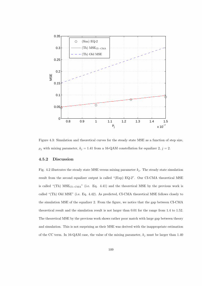
0.8 0.9 1 1.1 1.2 1.3 1.4 1.5
x 10−7
0
0.05
0.1
0.15
0.2
0.25
0.3
0.35
µj
MS
E
(Sim) EQ-2
(Th) MSECI−CMA
(Th) Old MSE
Figure 4.3: Simulation and theoretical curves for the steady state MSE as a function of step size,
µj with mixing parameter, kj = 1.41 from a 16-QAM constellation for equalizer 2, j = 2.
4.5.2 Discussion
Fig. 4.2 illustrates the steady state MSE versus mixing parameter kj . The steady state simulation
result from the second equalizer output is called “(Exp) EQ-2”. Our CI-CMA theoretical MSE
is called “(Th) MSECI−CMA” (i.e. Eq. 4.41) and the theoretical MSE by the previous work is
called “(Th) Old MSE” (i.e. Eq. 4.42). As predicted, CI-CMA theoretical MSE follows closely to
the simulation MSE of the equalizer 2. From the figure, we notice that the gap between CI-CMA
theoretical result and the simulation result is not larger than 0.01 for the range from 1.4 to 1.52.
The theoretical MSE by the previous work shows rather poor match with large gap between theory
and simulation. This is not surprising as their MSE was derived with the inappropriate estimation
of the CC term. In 16-QAM case, the value of the mixing parameter, kj must be larger than 1.40
109
in order to ensure source separation ability. From the figure, we can see that the steady state MSE
can be increased as kj increasing. Therefore, we suggest that kj = 1.41 should be chosen in order
to ensure source separation ability and also remain the lowest steady state MSE value.
Next, Fig. 4.3 presents the steady state MSE versus step size of the equalizer 2, µj . The
figure shows CI-CMA theoretical MSE follows closely to the simulation MSE of the equalizer 2
and a poorer match with the MSE of Eq. 4.42. Large value of step size is helpful to increase the
convergence rate, but it has been shown in the figure that it increases the MSE value as well. This
reveals the limitation of CI-CMA because the high convergence rate and low steady state MSE
cannot be achieved at the same time.
110
Chapter 5
Hybrid Algorithms for MIMO
Equalization
5.1 Introduction
High reliability communication link can be achieved through the reduction of the error rate at the
receiver. However, in the presence of noises, ISI and CCI, the error reduction is a challenging task
for the receiver. Therefore, we propose hybrid algorithms to improve the performance of MIMO
blind equalization algorithm. The hybrid algorithms are constructed by some blind algorithms. In
this chapter, we discuss the way of the hybrid algorithms have been constructed and then validate
the hybrid algorithms through simulations.
The chapter is structured as follows, In Section 5.2, the system model is briefly presented. In
Section 5.3, the general ways to hybrid the algorithms in MIMO equalization are shown. The
performance comparison among the hybrid algorithms and the previous works are presented in
Section 5.4 with discussions in Section 5.4.4.
111
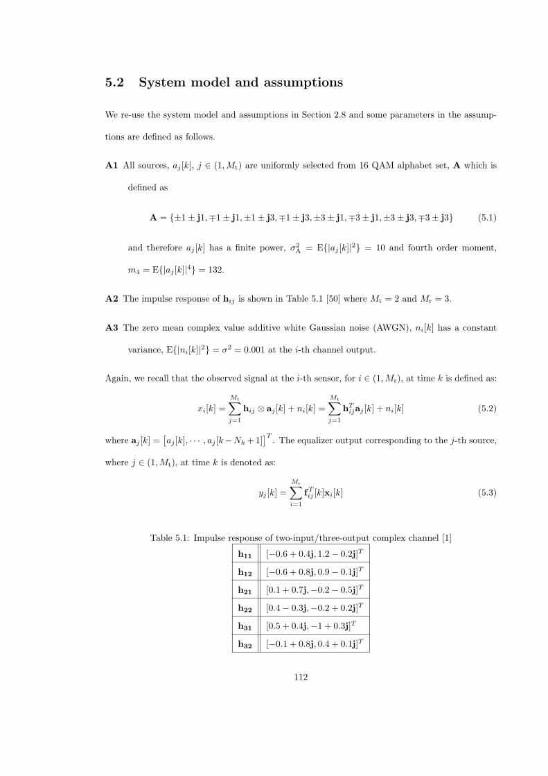
5.2 System model and assumptions
We re-use the system model and assumptions in Section 2.8 and some parameters in the assump-
tions are defined as follows.
A1 All sources, aj [k], j ∈ (1,Mt) are uniformly selected from 16 QAM alphabet set, A which is
defined as
A = ±1± j1,∓1± j1,±1± j3,∓1± j3,±3± j1,∓3± j1,±3± j3,∓3± j3 (5.1)
and therefore aj [k] has a finite power, σ2A = E|aj [k]|2 = 10 and fourth order moment,
m4 = E|aj [k]|4 = 132.
A2 The impulse response of hij is shown in Table 5.1 [50] where Mt = 2 and Mr = 3.
A3 The zero mean complex value additive white Gaussian noise (AWGN), ni[k] has a constant
variance, E|ni[k]|2 = σ2 = 0.001 at the i-th channel output.
Again, we recall that the observed signal at the i-th sensor, for i ∈ (1,Mr), at time k is defined as:
xi[k] =
Mt∑j=1
hij ⊗ aj [k] + ni[k] =
Mt∑j=1
hTijaj [k] + ni[k] (5.2)
where aj [k] =[aj [k], · · · , aj [k−Nh+1]
]T. The equalizer output corresponding to the j-th source,
where j ∈ (1,Mt), at time k is denoted as:
yj [k] =
Mr∑i=1
fTij [k]xi[k] (5.3)
Table 5.1: Impulse response of two-input/three-output complex channel [1]
h11 [−0.6 + 0.4j, 1.2− 0.2j]T
h12 [−0.6 + 0.8j, 0.9− 0.1j]T
h21 [0.1 + 0.7j,−0.2− 0.5j]T
h22 [0.4− 0.3j,−0.2 + 0.2j]T
h31 [0.5 + 0.4j,−1 + 0.3j]T
h32 [−0.1 + 0.8j, 0.4 + 0.1j]T
112
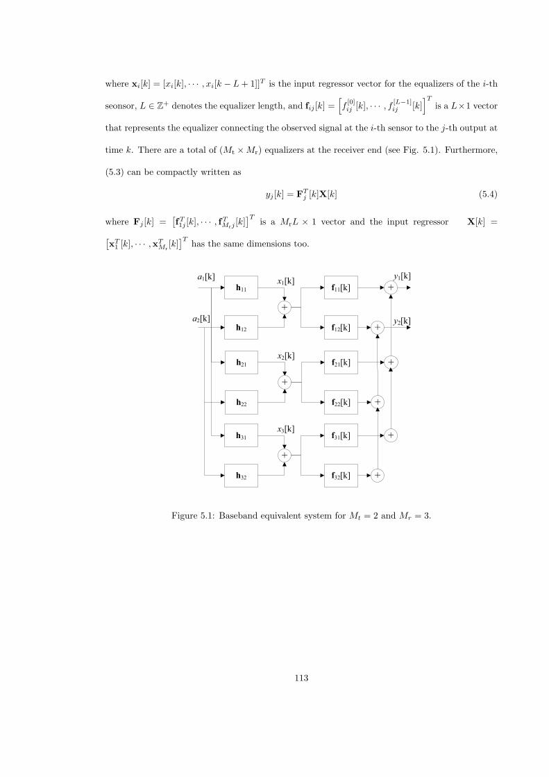
where xi[k] = [xi[k], · · · , xi[k − L+ 1]]T is the input regressor vector for the equalizers of the i-th
seonsor, L ∈ Z+ denotes the equalizer length, and fij [k] =[f[0]ij [k], · · · , f [L−1]
ij [k]]T
is a L×1 vector
that represents the equalizer connecting the observed signal at the i-th sensor to the j-th output at
time k. There are a total of (Mt ×Mr) equalizers at the receiver end (see Fig. 5.1). Furthermore,
(5.3) can be compactly written as
yj [k] = FTj [k]X[k] (5.4)
where Fj [k] =[fT1j [k], · · · , fTMrj
[k]]T
is a MrL × 1 vector and the input regressor X[k] =[xT1 [k], · · · ,xT
Mr[k]]T
has the same dimensions too.
h11
a1[k]
f11[k]
+
h12 f12[k]
+
+a2[k]
x1[k]y1[k]
y2[k]
h21 f21[k]
+
h22 f22[k]
+
+
x2[k]
h31 f31[k]
+
h32 f32[k]
+
+
x3[k]
Figure 5.1: Baseband equivalent system for Mt = 2 and Mr = 3.
113
5.3 Blind Adaptive Hybrid Algorithms For MIMO Systems
A hybrid algorithm that is employed by the MIMO linear equalizer is called that way because it
opens the channel eye using an acquisition algorithm, a new Adaptive Constant Modulus Algo-
rithm (ACMA), tracks the channel (after the channel eye is open) using a decision directed (DD)
algorithm, and perform source separation algorithm using a cross correlation function (CC). The
acquisition and source separation algorithm can open the channel eye and ensure the outputs are
mutually uncorrelated but usually yields large steady state errors. That is why hybrid algorithms
couple the acquisition and source separation algorithms with a tracking algorithm (e.g. DD algo-
rithm) to exploit the discrete nature of the input data to achieve much lower error rates. To the
best of the author’s knowledge, such algorithms have not been purposed for the MIMO system,
even though a similar idea can be found in SISO system. We emphasize that the migration of some
hybrid algorithms from the SISO to MIMO systems, although may seem straight forward initially,
often results in divergence unless a very small step size (which is undesirable because it slows con-
vergence) is used. To overcome the issue, we will propose a new acquisition algorithm. Instead of
that, the past SISO approaches are not equipped with source separation algorithm, therefore, the
past approaches cannot perform source separation. Our approach in this chapter is to propose the
new hybrid algorithms that can open the channel eye, performance source separation and produce
significant low steady state MSE.
In what follows, we will provide a general cost function that we employ in our hybrid algorithms.
The update equations are also provided thereafter.
5.3.1 General cost function
In this section, we define the general cost function of hybrid algorithm and then present the
stochastic gradient descent algorithm (SGA).
For simplicity, we consider two sources (i.e. Mt = 2) case. J1[k] and J2[k] are denoted as the
cost functions of the equalizer output 1 and 2 respectively. Furthermore, the j-th cost function,
114
Jj [k] where j = 1, 2 is defined as
Jj [k] =1
2E|ϵj [k]|2
(5.5)
where ϵj is known as equalization error function that is a function of j-th equalizer output, yj [k].
In practice, we use SGA to minimize the cost function 5.5. As a result, the equalizer coefficients
after dropping E. are updated as below:
Fj [k + 1] = Fj [k]− µjϵj [k]X∗[k] (5.6)
where µj is a suitable step size value for the j-th equalizer output andX∗[k] =[xT1 [k],x
T2 [k], ...,x
TM [k]
]His a MrL× 1 vector. Finally, yj [k] can be obtained as Eq. 5.4.
We emphasize that the main distinction among the hybrid algorithms is the error function,
ϵj [k] in Eq. 5.6. Therefore, we will concentrate on ϵj [k] in the below section.
5.3.2 Acquisition, Source Separation and Tracking algorithms
The acquisition, source separation and tracking algorithms are the single task algorithms that will
be combined as hybrid algorithms. Therefore, we describe the single task algorithms before the
description of hybrid algorithms.
In order to open the channel eye, the acquisition algorithm must be employed. In this case, we
propose a new acquisition algorithm, which is call adaptive constant modulus algorithm (ACMA)
as the acquisition algorithm. ACMA is different with the conventional CMA because adaptive
dispersion value is used in ACMA instead of fixed value. The error functions of acquisition (i.e.
eacq,j [k]) and ACMA (i.e. eACMA,j [k]) for j-th equalizer are defined as
eacq,j [k] = eACMA,j [k] = (|yj [k]|2 − Rj[k])yj [k] (5.7)
where the adaptive dispersion is defined as
Rj[k + 1] = Rj[k]− 0.001(|yj [k]|2 − σ2
A
)(5.8)
115
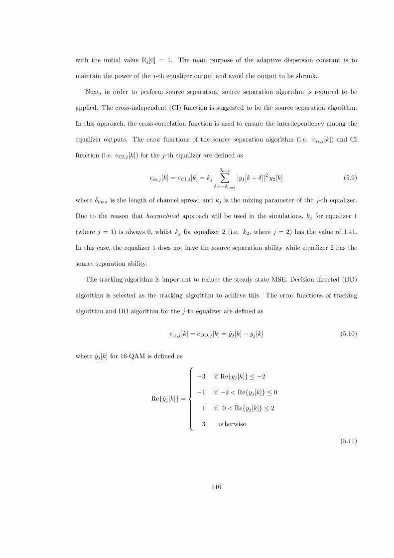
with the initial value Rj[0] = 1. The main purpose of the adaptive dispersion constant is to
maintain the power of the j-th equalizer output and avoid the output to be shrunk.
Next, in order to perform source separation, source separation algorithm is required to be
applied. The cross-independent (CI) function is suggested to be the source separation algorithm.
In this approach, the cross-correlation function is used to ensure the interdependency among the
equalizer outputs. The error functions of the source separation algorithm (i.e. ess,j [k]) and CI
function (i.e. eCI,j [k]) for the j-th equalizer are defined as
ess,j [k] = eCI,j [k] = kj
δmax∑δ=−δmax
|y1[k − δ]|2 y2[k] (5.9)
where δmax is the length of channel spread and kj is the mixing parameter of the j-th equalizer.
Due to the reason that hierarchical approach will be used in the simulations, kj for equalizer 1
(where j = 1) is always 0, whilst kj for equalizer 2 (i.e. k2, where j = 2) has the value of 1.41.
In this case, the equalizer 1 does not have the source separation ability while equalizer 2 has the
source separation ability.
The tracking algorithm is important to reduce the steady state MSE. Decision directed (DD)
algorithm is selected as the tracking algorithm to achieve this. The error functions of tracking
algorithm and DD algorithm for the j-th equalizer are defined as
etr,j [k] = eDD,j [k] = yj [k]− yj [k] (5.10)
where yj [k] for 16-QAM is defined as
Reyj [k] =
−3 if Reyj [k] ≤ −2
−1 if −2 < Reyj [k] ≤ 0
1 if 0 < Reyj [k] ≤ 2
3 otherwise
(5.11)
116
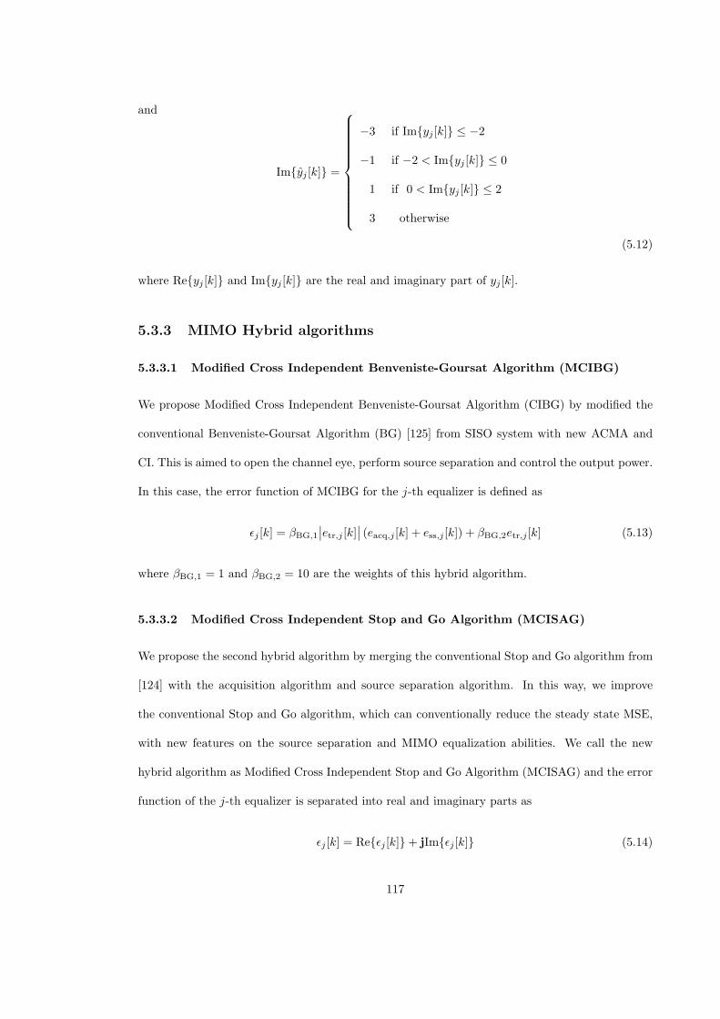
and
Imyj [k] =
−3 if Imyj [k] ≤ −2
−1 if −2 < Imyj [k] ≤ 0
1 if 0 < Imyj [k] ≤ 2
3 otherwise
(5.12)
where Reyj [k] and Imyj [k] are the real and imaginary part of yj [k].
5.3.3 MIMO Hybrid algorithms
5.3.3.1 Modified Cross Independent Benveniste-Goursat Algorithm (MCIBG)
We propose Modified Cross Independent Benveniste-Goursat Algorithm (CIBG) by modified the
conventional Benveniste-Goursat Algorithm (BG) [125] from SISO system with new ACMA and
CI. This is aimed to open the channel eye, perform source separation and control the output power.
In this case, the error function of MCIBG for the j-th equalizer is defined as
ϵj [k] = βBG,1
∣∣etr,j [k]∣∣ (eacq,j [k] + ess,j [k]) + βBG,2etr,j [k] (5.13)
where βBG,1 = 1 and βBG,2 = 10 are the weights of this hybrid algorithm.
5.3.3.2 Modified Cross Independent Stop and Go Algorithm (MCISAG)
We propose the second hybrid algorithm by merging the conventional Stop and Go algorithm from
[124] with the acquisition algorithm and source separation algorithm. In this way, we improve
the conventional Stop and Go algorithm, which can conventionally reduce the steady state MSE,
with new features on the source separation and MIMO equalization abilities. We call the new
hybrid algorithm as Modified Cross Independent Stop and Go Algorithm (MCISAG) and the error
function of the j-th equalizer is separated into real and imaginary parts as
ϵj [k] = Reϵj [k]+ jImϵj [k] (5.14)
117
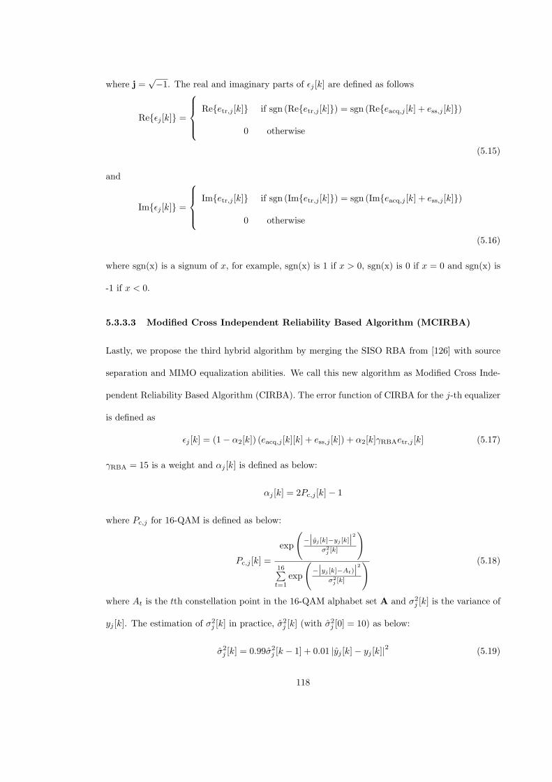
where j =√−1. The real and imaginary parts of ϵj [k] are defined as follows
Reϵj [k] =
Reetr,j [k] if sgn (Reetr,j [k]) = sgn (Reeacq,j [k] + ess,j [k])
0 otherwise
(5.15)
and
Imϵj [k] =
Imetr,j [k] if sgn (Imetr,j [k]) = sgn (Imeacq,j [k] + ess,j [k])
0 otherwise
(5.16)
where sgn(x) is a signum of x, for example, sgn(x) is 1 if x > 0, sgn(x) is 0 if x = 0 and sgn(x) is
-1 if x < 0.
5.3.3.3 Modified Cross Independent Reliability Based Algorithm (MCIRBA)
Lastly, we propose the third hybrid algorithm by merging the SISO RBA from [126] with source
separation and MIMO equalization abilities. We call this new algorithm as Modified Cross Inde-
pendent Reliability Based Algorithm (CIRBA). The error function of CIRBA for the j-th equalizer
is defined as
ϵj [k] = (1− α2[k]) (eacq,j [k][k] + ess,j [k]) + α2[k]γRBAetr,j [k] (5.17)
γRBA = 15 is a weight and αj [k] is defined as below:
αj [k] = 2Pc,j [k]− 1
where Pc,j for 16-QAM is defined as below:
Pc,j [k] =
exp
(−∣∣yj [k]−yj [k]
∣∣2σ2j [k]
)16∑t=1
exp
(−∣∣yj [k]−At)
∣∣2σ2j [k]
) (5.18)
where At is the tth constellation point in the 16-QAM alphabet set A and σ2j [k] is the variance of
yj [k]. The estimation of σ2j [k] in practice, σ2
j [k] (with σ2j [0] = 10) as below:
σ2j [k] = 0.99σ2
j [k − 1] + 0.01 |yj [k]− yj [k]|2 (5.19)
118
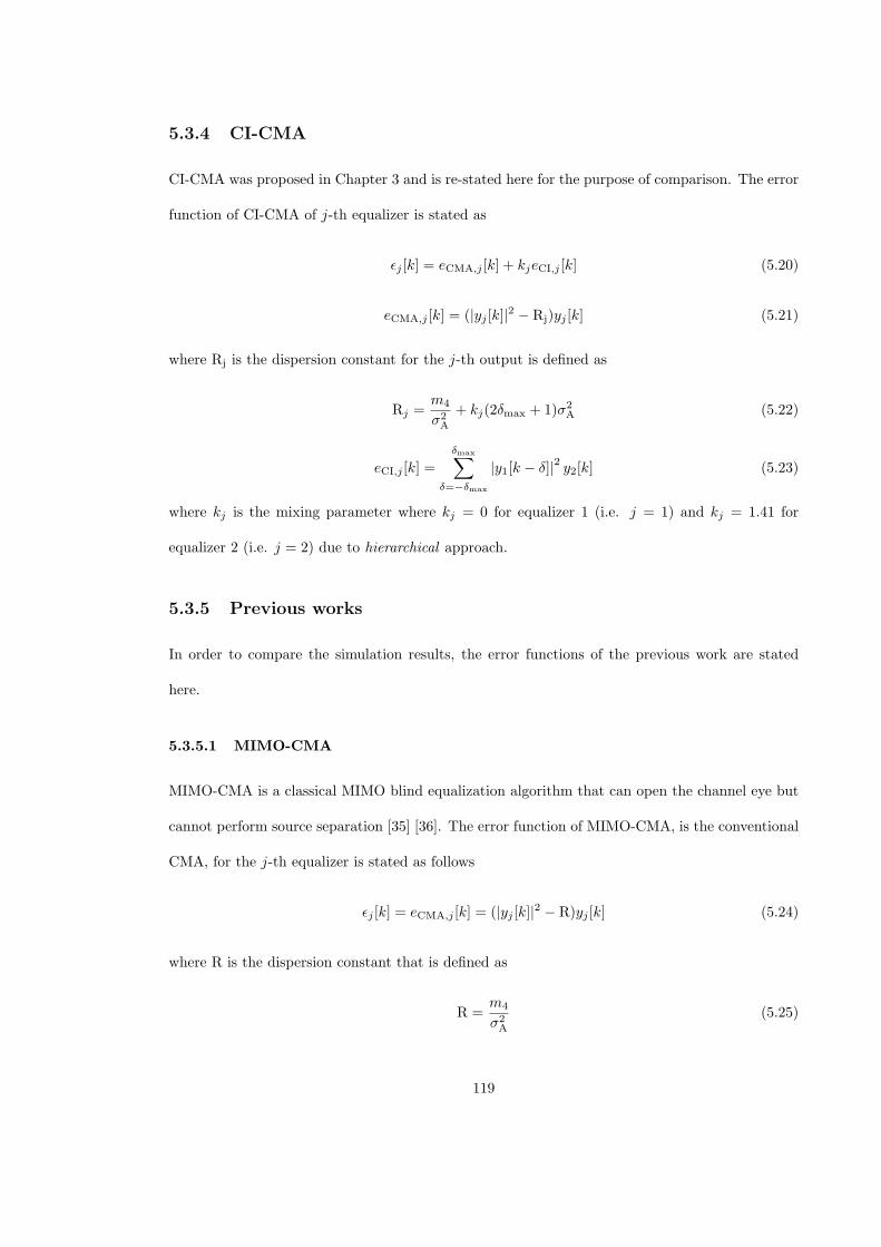
5.3.4 CI-CMA
CI-CMA was proposed in Chapter 3 and is re-stated here for the purpose of comparison. The error
function of CI-CMA of j-th equalizer is stated as
ϵj [k] = eCMA,j [k] + kjeCI,j [k] (5.20)
eCMA,j [k] = (|yj [k]|2 − Rj)yj [k] (5.21)
where Rj is the dispersion constant for the j-th output is defined as
Rj =m4
σ2A
+ kj(2δmax + 1)σ2A (5.22)
eCI,j [k] =
δmax∑δ=−δmax
|y1[k − δ]|2 y2[k] (5.23)
where kj is the mixing parameter where kj = 0 for equalizer 1 (i.e. j = 1) and kj = 1.41 for
equalizer 2 (i.e. j = 2) due to hierarchical approach.
5.3.5 Previous works
In order to compare the simulation results, the error functions of the previous work are stated
here.
5.3.5.1 MIMO-CMA
MIMO-CMA is a classical MIMO blind equalization algorithm that can open the channel eye but
cannot perform source separation [35] [36]. The error function of MIMO-CMA, is the conventional
CMA, for the j-th equalizer is stated as follows
ϵj [k] = eCMA,j [k] = (|yj [k]|2 − R)yj [k] (5.24)
where R is the dispersion constant that is defined as
R =m4
σ2A
(5.25)
119
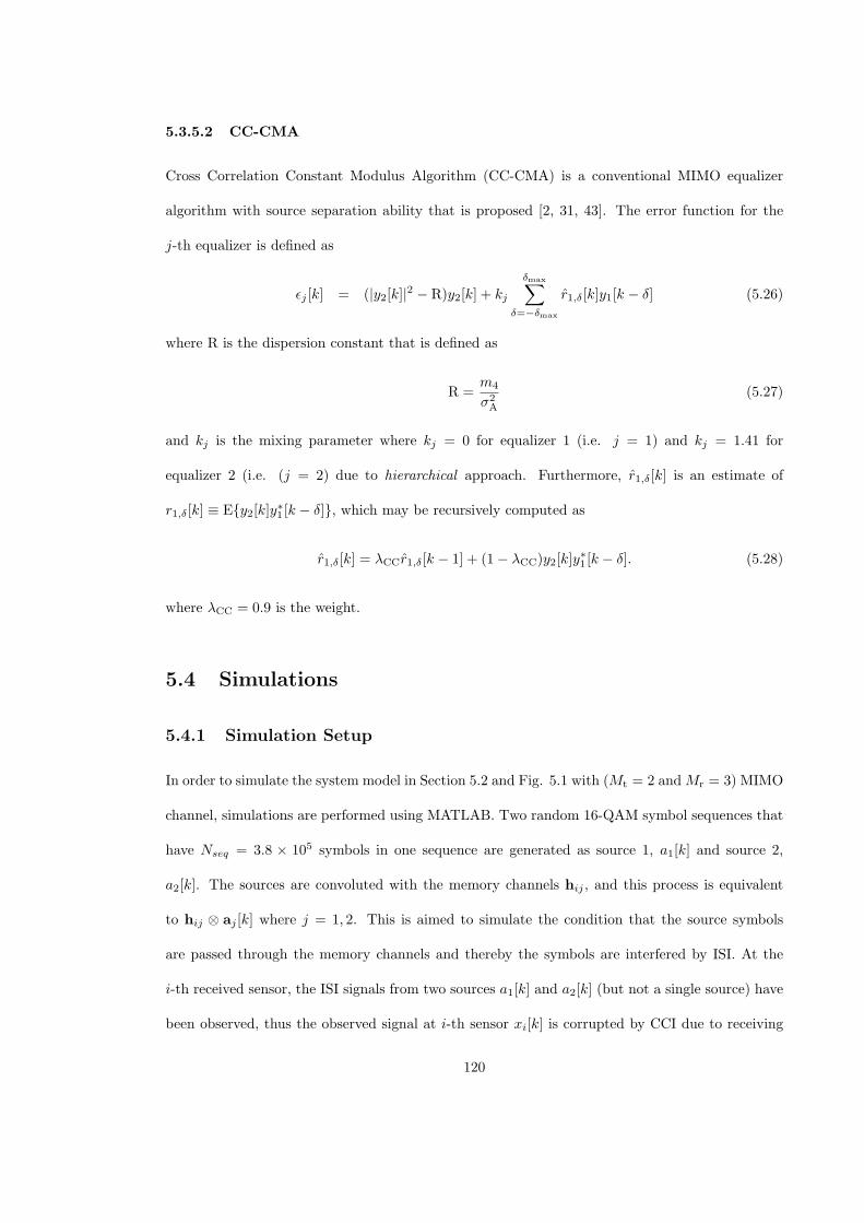
5.3.5.2 CC-CMA
Cross Correlation Constant Modulus Algorithm (CC-CMA) is a conventional MIMO equalizer
algorithm with source separation ability that is proposed [2, 31, 43]. The error function for the
j-th equalizer is defined as
ϵj [k] = (|y2[k]|2 − R)y2[k] + kj
δmax∑δ=−δmax
r1,δ[k]y1[k − δ] (5.26)
where R is the dispersion constant that is defined as
R =m4
σ2A
(5.27)
and kj is the mixing parameter where kj = 0 for equalizer 1 (i.e. j = 1) and kj = 1.41 for
equalizer 2 (i.e. (j = 2) due to hierarchical approach. Furthermore, r1,δ[k] is an estimate of
r1,δ[k] ≡ Ey2[k]y∗1 [k − δ], which may be recursively computed as
r1,δ[k] = λCCr1,δ[k − 1] + (1− λCC)y2[k]y∗1 [k − δ]. (5.28)
where λCC = 0.9 is the weight.
5.4 Simulations
5.4.1 Simulation Setup
In order to simulate the system model in Section 5.2 and Fig. 5.1 with (Mt = 2 andMr = 3) MIMO
channel, simulations are performed using MATLAB. Two random 16-QAM symbol sequences that
have Nseq = 3.8 × 10⁵ symbols in one sequence are generated as source 1, a1[k] and source 2,
a2[k]. The sources are convoluted with the memory channels hij , and this process is equivalent
to hij ⊗ aj [k] where j = 1, 2. This is aimed to simulate the condition that the source symbols
are passed through the memory channels and thereby the symbols are interfered by ISI. At the
i-th received sensor, the ISI signals from two sources a1[k] and a2[k] (but not a single source) have
been observed, thus the observed signal at i-th sensor xi[k] is corrupted by CCI due to receiving
120
two sources and ISI due to memory channels. Instead of that, a random zero mean complex value
additive white Gaussian noises (AWGN), ni[k] that have the power of E|ni[k]|2 = σ2 = 0.001
are generated and summed with the the observed signal at i-th sensor xi[k]. In this cases, the
observed signal at i-th sensor xi[k] is not only corrupted by interferences, but also is distorted by
noises. This scenario can be simulated through computing Eq. 5.2 and the impulse responses of
channels hij are stated in Table 5.1.
Next, to simulate the equalization process, we will test using the hierarchical approach, i.e.,
the first equalizer is allowed to recover any of the two sources (usually the stronger one) and the
second equalizer should be able to avoid the extracted source by the first equalizer if BSS works.
In this case, equalizer 1 uses the algorithm without source separation ability, whilst equalizer 2
uses the algorithm that has source separation ability (except the case of MIMO-CMA algorithm).
The filter weights f11[0] and f22[0] are initialized with a center spike [36] whilst fij [0], ∀i = j,
are initialized with zero-vectors. After the initialization, the observed signals xi[k] are fed through
the filters Fj [k], which is the concatenation vector by several filters fij [k], and generated the two
outputs yj [k] where j = 1, 2 because two sources were transmitted. This can be achieved executing
the output equation in Eq. 5.4. At the same time, the filter vector Fj [k] are iteratively updated
for every time k through computing the filter update equation in Eq. 5.6.
In order to simulate an algorithm, the general error function, ϵj [k] that is located inside the
filter update equation (i.e. Eq. 5.6) is replaced by the correspond error function of the algorithm.
Therefore, to perform simulation on MIMO-CMA, we uses the error function in Eq. 5.24 to update
the filter update equation (i.e. Eq. 5.6). Similarly, the simulation is repeated for CC-CMA (i.e.
Eq. 5.26), CI-CMA (i.e. Eq. 5.20), MCIBG (i.e. Eq. 5.13), MCIRBA (i.e. Eq. 5.17) and MCISAG
(i.e. Eq. 5.14).
Regarding to the simulation parameters, the filter length L = 3 and channel spread length
δmax = 4 are assigned. The step sizes of equalizer 1 and 2 are empirically chosen. This means
several simulations have been run to find the step sizes that can avoid divergence. The step size of
121
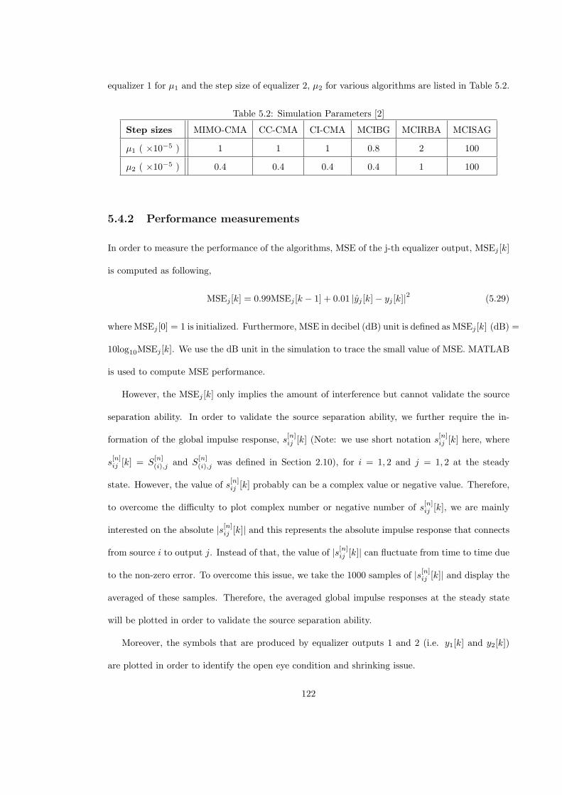
equalizer 1 for µ1 and the step size of equalizer 2, µ2 for various algorithms are listed in Table 5.2.
Table 5.2: Simulation Parameters [2]
Step sizes MIMO-CMA CC-CMA CI-CMA MCIBG MCIRBA MCISAG
µ1 ( ×10−5 ) 1 1 1 0.8 2 100
µ2 ( ×10−5 ) 0.4 0.4 0.4 0.4 1 100
5.4.2 Performance measurements
In order to measure the performance of the algorithms, MSE of the j-th equalizer output, MSEj [k]
is computed as following,
MSEj [k] = 0.99MSEj [k − 1] + 0.01 |yj [k]− yj [k]|2 (5.29)
where MSEj [0] = 1 is initialized. Furthermore, MSE in decibel (dB) unit is defined as MSEj [k] (dB) =
10log10MSEj [k]. We use the dB unit in the simulation to trace the small value of MSE. MATLAB
is used to compute MSE performance.
However, the MSEj [k] only implies the amount of interference but cannot validate the source
separation ability. In order to validate the source separation ability, we further require the in-
formation of the global impulse response, s[n]ij [k] (Note: we use short notation s
[n]ij [k] here, where
s[n]ij [k] = S
[n](i),j and S
[n](i),j was defined in Section 2.10), for i = 1, 2 and j = 1, 2 at the steady
state. However, the value of s[n]ij [k] probably can be a complex value or negative value. Therefore,
to overcome the difficulty to plot complex number or negative number of s[n]ij [k], we are mainly
interested on the absolute |s[n]ij [k]| and this represents the absolute impulse response that connects
from source i to output j. Instead of that, the value of |s[n]ij [k]| can fluctuate from time to time due
to the non-zero error. To overcome this issue, we take the 1000 samples of |s[n]ij [k]| and display the
averaged of these samples. Therefore, the averaged global impulse responses at the steady state
will be plotted in order to validate the source separation ability.
Moreover, the symbols that are produced by equalizer outputs 1 and 2 (i.e. y1[k] and y2[k])
are plotted in order to identify the open eye condition and shrinking issue.
122
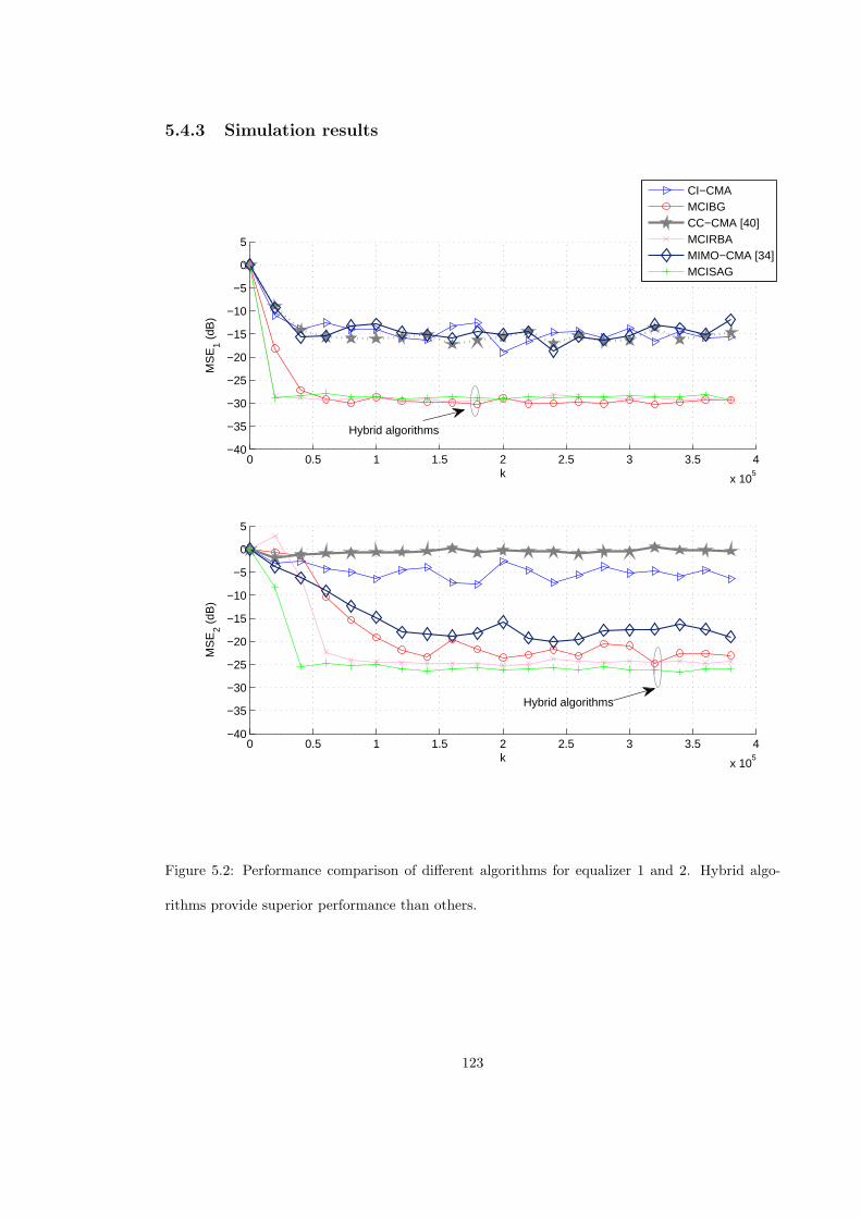
5.4.3 Simulation results
0 0.5 1 1.5 2 2.5 3 3.5 4
x 105
−40
−35
−30
−25
−20
−15
−10
−5
0
5
MS
E1 (
dB)
k
0 0.5 1 1.5 2 2.5 3 3.5 4
x 105
−40
−35
−30
−25
−20
−15
−10
−5
0
5
MS
E2 (
dB)
k
CI−CMAMCIBGCC−CMA [40]MCIRBAMIMO−CMA [34]MCISAG
Hybrid algorithms
Hybrid algorithms
Figure 5.2: Performance comparison of different algorithms for equalizer 1 and 2. Hybrid algo-
rithms provide superior performance than others.
123
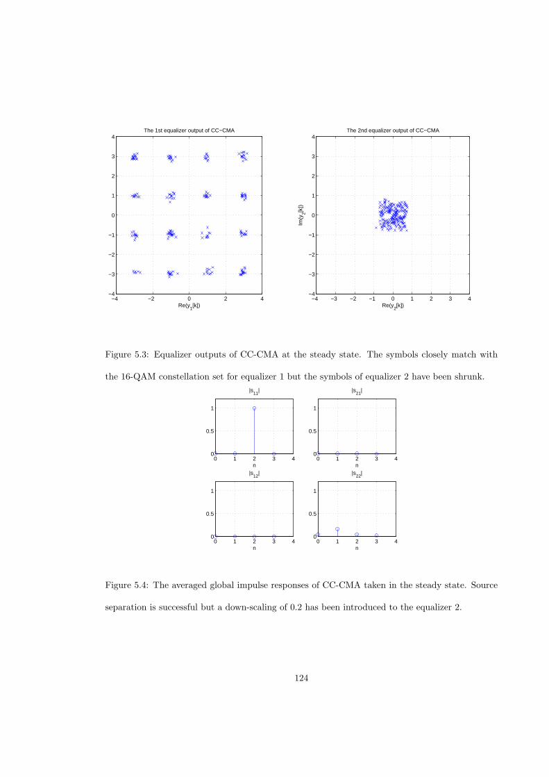
−4 −2 0 2 4−4
−3
−2
−1
0
1
2
3
4
Re(y1[k])
The 1st equalizer output of CC−CMA
−4 −3 −2 −1 0 1 2 3 4−4
−3
−2
−1
0
1
2
3
4
Im(y
2[k])
Re(y2[k])
The 2nd equalizer output of CC−CMA
Figure 5.3: Equalizer outputs of CC-CMA at the steady state. The symbols closely match with
the 16-QAM constellation set for equalizer 1 but the symbols of equalizer 2 have been shrunk.
0 1 2 3 40
0.5
1
n
|s11
|
0 1 2 3 40
0.5
1
n
|s21
|
0 1 2 3 40
0.5
1
n
|s12
|
0 1 2 3 40
0.5
1
n
|s22
|
Figure 5.4: The averaged global impulse responses of CC-CMA taken in the steady state. Source
separation is successful but a down-scaling of 0.2 has been introduced to the equalizer 2.
124
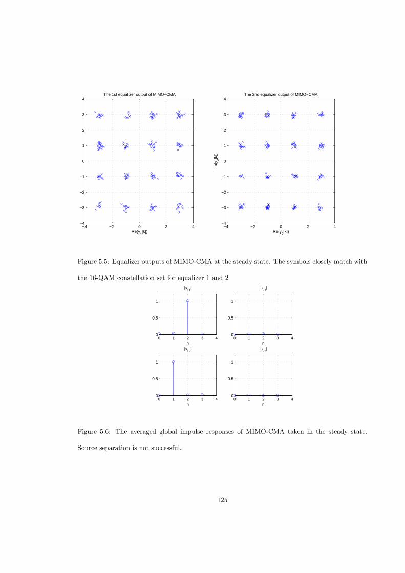
−4 −2 0 2 4−4
−3
−2
−1
0
1
2
3
4
Re(y1[k])
The 1st equalizer output of MIMO−CMA
−4 −2 0 2 4−4
−3
−2
−1
0
1
2
3
4
Im(y
2[k])
Re(y2[k])
The 2nd equalizer output of MIMO−CMA
Figure 5.5: Equalizer outputs of MIMO-CMA at the steady state. The symbols closely match with
the 16-QAM constellation set for equalizer 1 and 2
0 1 2 3 40
0.5
1
n
|s11
|
0 1 2 3 40
0.5
1
n
|s21
|
0 1 2 3 40
0.5
1
n
|s12
|
0 1 2 3 40
0.5
1
n
|s22
|
Figure 5.6: The averaged global impulse responses of MIMO-CMA taken in the steady state.
Source separation is not successful.
125
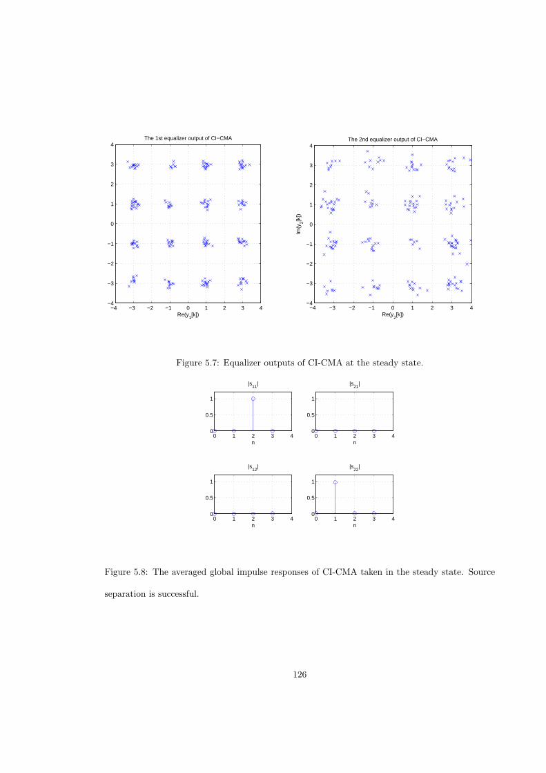
−4 −3 −2 −1 0 1 2 3 4−4
−3
−2
−1
0
1
2
3
4
Re(y1[k])
The 1st equalizer output of CI−CMA
−4 −3 −2 −1 0 1 2 3 4−4
−3
−2
−1
0
1
2
3
4
Re(y2[k])
Im(y
2[k])
The 2nd equalizer output of CI−CMA
Figure 5.7: Equalizer outputs of CI-CMA at the steady state.
0 1 2 3 40
0.5
1
n
|s11
|
0 1 2 3 40
0.5
1
n
|s21
|
0 1 2 3 40
0.5
1
n
|s12
|
0 1 2 3 40
0.5
1
n
|s22
|
Figure 5.8: The averaged global impulse responses of CI-CMA taken in the steady state. Source
separation is successful.
126
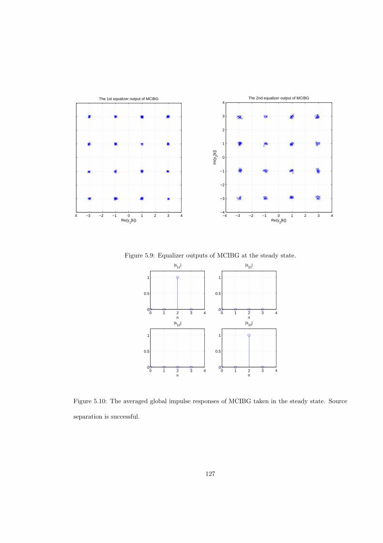
−4 −3 −2 −1 0 1 2 3 4−4
−3
−2
−1
0
1
2
3
4
Re(y1[k])
The 1st equalizer output of MCIBG
−4 −3 −2 −1 0 1 2 3 4−4
−3
−2
−1
0
1
2
3
4
Im(y
2[k])
Re(y2[k])
The 2nd equalizer output of MCIBG
Figure 5.9: Equalizer outputs of MCIBG at the steady state.
0 1 2 3 40
0.5
1
n
|s11
|
0 1 2 3 40
0.5
1
n
|s21
|
0 1 2 3 40
0.5
1
n
|s12
|
0 1 2 3 40
0.5
1
n
|s22
|
Figure 5.10: The averaged global impulse responses of MCIBG taken in the steady state. Source
separation is successful.
127
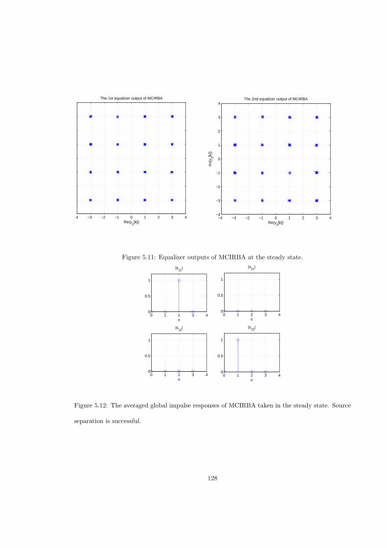
−4 −3 −2 −1 0 1 2 3 4−4
−3
−2
−1
0
1
2
3
4
Re(y1[k])
The 1st equalizer output of MCIRBA
−4 −3 −2 −1 0 1 2 3 4−4
−3
−2
−1
0
1
2
3
4
Im(y
2[k])
Re(y2[k])
The 2nd equalizer output of MCIRBA
Figure 5.11: Equalizer outputs of MCIRBA at the steady state.
0 1 2 3 40
0.5
1
n
|s11
|
0 1 2 3 40
0.5
1
n
|s21
|
0 1 2 3 40
0.5
1
n
|s12
|
0 1 2 3 40
0.5
1
n
|s22
|
Figure 5.12: The averaged global impulse responses of MCIRBA taken in the steady state. Source
separation is successful.
128
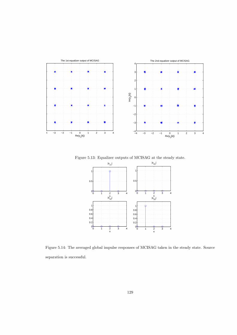
−4 −3 −2 −1 0 1 2 3 4−4
−3
−2
−1
0
1
2
3
4
Re(y1[k])
The 1st equalizer output of MCISAG
−4 −3 −2 −1 0 1 2 3 4−4
−3
−2
−1
0
1
2
3
4
Im(y
2[k])
Re(y2[k])
The 2nd equalizer output of MCISAG
Figure 5.13: Equalizer outputs of MCISAG at the steady state.
0 1 2 3 40
0.5
1
n
|s11
|
0 1 2 3 40
0.5
1
n
|s21
|
0 1 2 3 40
0.2
0.4
0.6
0.8
1
n
|s12
|
0 1 2 3 40
0.2
0.4
0.6
0.8
1
n
|s22
|
Figure 5.14: The averaged global impulse responses of MCISAG taken in the steady state. Source
separation is successful.
129
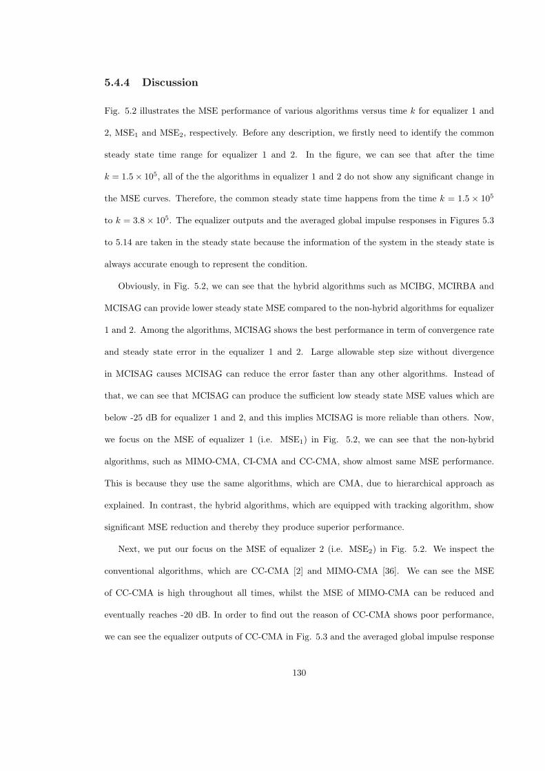
5.4.4 Discussion
Fig. 5.2 illustrates the MSE performance of various algorithms versus time k for equalizer 1 and
2, MSE1 and MSE2, respectively. Before any description, we firstly need to identify the common
steady state time range for equalizer 1 and 2. In the figure, we can see that after the time
k = 1.5× 10⁵, all of the the algorithms in equalizer 1 and 2 do not show any significant change in
the MSE curves. Therefore, the common steady state time happens from the time k = 1.5 × 10⁵
to k = 3.8× 10⁵. The equalizer outputs and the averaged global impulse responses in Figures 5.3
to 5.14 are taken in the steady state because the information of the system in the steady state is
always accurate enough to represent the condition.
Obviously, in Fig. 5.2, we can see that the hybrid algorithms such as MCIBG, MCIRBA and
MCISAG can provide lower steady state MSE compared to the non-hybrid algorithms for equalizer
1 and 2. Among the algorithms, MCISAG shows the best performance in term of convergence rate
and steady state error in the equalizer 1 and 2. Large allowable step size without divergence
in MCISAG causes MCISAG can reduce the error faster than any other algorithms. Instead of
that, we can see that MCISAG can produce the sufficient low steady state MSE values which are
below -25 dB for equalizer 1 and 2, and this implies MCISAG is more reliable than others. Now,
we focus on the MSE of equalizer 1 (i.e. MSE1) in Fig. 5.2, we can see that the non-hybrid
algorithms, such as MIMO-CMA, CI-CMA and CC-CMA, show almost same MSE performance.
This is because they use the same algorithms, which are CMA, due to hierarchical approach as
explained. In contrast, the hybrid algorithms, which are equipped with tracking algorithm, show
significant MSE reduction and thereby they produce superior performance.
Next, we put our focus on the MSE of equalizer 2 (i.e. MSE2) in Fig. 5.2. We inspect the
conventional algorithms, which are CC-CMA [2] and MIMO-CMA [36]. We can see the MSE
of CC-CMA is high throughout all times, whilst the MSE of MIMO-CMA can be reduced and
eventually reaches -20 dB. In order to find out the reason of CC-CMA shows poor performance,
we can see the equalizer outputs of CC-CMA in Fig. 5.3 and the averaged global impulse response
130
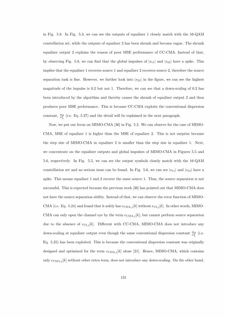
in Fig. 5.8. In Fig. 5.3, we can see the outputs of equalizer 1 closely match with the 16-QAM
constellation set, while the outputs of equalizer 2 has been shrunk and become vague. The shrunk
equalizer output 2 explains the reason of poor MSE performance of CC-CMA. Instead of that,
by observing Fig. 5.8, we can find that the global impulses of |s11| and |s22| have a spike. This
implies that the equalizer 1 recovers source 1 and equalizer 2 recovers source 2, therefore the source
separation task is fine. However, we further look into |s22| in the figure, we can see the highest
magnitude of the impulse is 0.2 but not 1. Therefore, we can see that a down-scaling of 0.2 has
been introduced by the algorithm and thereby causes the shrunk of equalizer output 2 and then
produces poor MSE performance. This is because CC-CMA exploits the conventional dispersion
constant, m4
σ2A
(i.e. Eq .5.27) and the detail will be explained in the next paragraph.
Now, we put our focus on MIMO-CMA [36] in Fig. 5.2. We can observe for the case of MIMO-
CMA, MSE of equalizer 1 is higher than the MSE of equalizer 2. This is not surprise because
the step size of MIMO-CMA in equalizer 2 is smaller than the step size in equalizer 1. Next,
we concentrate on the equalizer outputs and global impulses of MIMO-CMA in Figures 5.5 and
5.6, respectively. In Fig. 5.5, we can see the output symbols closely match with the 16-QAM
constellation set and no serious issue can be found. In Fig. 5.6, we can see |s11| and |s12| have a
spike. This means equalizer 1 and 2 recover the same source 1. Thus, the source separation is not
successful. This is expected because the previous work [36] has pointed out that MIMO-CMA does
not have the source separation ability. Instead of that, we can observe the error function of MIMO-
CMA (i.e. Eq. 5.24) and found that it solely has eCMA,j [k] without eCI,j [k]. In other words, MIMO-
CMA can only open the channel eye by the term eCMA,j [k], but cannot perform source separation
due to the absence of eCI,j [k]. Different with CC-CMA, MIMO-CMA does not introduce any
down-scaling at equalizer output even though the same conventional dispersion constant m4
σ2A
(i.e.
Eq. 5.25) has been exploited. This is because the conventional dispersion constant was originally
designed and optimized for the term eCMA,j [k] alone [21]. Hence, MIMO-CMA, which contains
only eCMA,j [k] without other extra term, does not introduce any down-scaling. On the other hand,
131
CC-CMA has an extra term of “kjδmax∑
δ=−δmax
r1,δ[k]y1[k − δ]” for source separation in Eq. 5.26, but
the conventional dispersion constant, which was initially designed without considering the extra
term, has been exploited in CC-CMA. Therefore, due to the inappropriate dispersion constant has
been exploited, CC-CMA introduces down-scaling at equalizer output.
Now, we put our attention on CI-CMA. In Fig. 5.2, we can see CI-CMA shows relatively high
MSE values in equalizer 1 and 2. This is expected because CI-CMA only has the ability of open
eye and source separation, but it does not been equipped with the tracking algorithm. Next, we
put the target on the equalizer outputs and global impulses of CI-CMA in Figures 5.7 and 5.8,
respectively. In Fig. 5.7, the symbols of equalizer 1 and 2 match with the 16-QAM constellation
set. We can further observe that the symbols of equalizer 2 is more scattering than equalizer 1.
This is because, due to the hieratical approach, the equalizer 2 has an extra source separation
algorithm and thus produce high error rate. In Fig. 5.8, we can see a spike can be found in |s11|
and |s22|. This implies equalizer 1 retrieves source 1 and equalizer 2 retrieves source 2. Thus,
source separation is achieved as expected. Furthermore, different with CC-CMA, no down-scaling
can be found in CI-CMA because of new dispersion value in Eq. 5.22 has been used.
In Fig. 5.2, especially MSE of equalizer 1, we can observe the hybrid algorithms have almost
same MSE value after time k = 1 × 10⁵. This is because in this low error condition, the tracking
algorithms that are within the hybrid algorithms are almost dominant the hybrid algorithms. Due
to the reason that the hybrid algorithms use the same tracking algorithms (i.e. decision directed
algorithms), the hybrid algorithms show the almost same results after time k = 1× 10⁵. This case
can also be applied on the MCISAG and MCIRBA in equalizer 2. Instead of that, in the MSE
of equalizer 2, we can see MCIBG always shows higher MSE value than MCISAG and MCIRBA.
This is because the coexistence of tracking, source separation and acquisition algorithm in the error
function of MCIBG causes MCIBG is more sensitive to error compared to MCISAG and MCIRBA.
We put our focus on the the equalizer outputs and global impulses of hybrid algorithms. We
check the equalizer outputs of hybrid algorithms in Figures 5.9, 5.11 and 5.13. The symbols of
132
equalizer 1 and 2 of the hybrid algorithms show closely match with the 16-QAM constellation set
and no serious issue can be traced. In Fig. 5.9, we can see the symbols of equalizer 2 for MCIBG
is slightly scatter than the outputs of other hybrid algorithms. This is because MCIBG is more
sensitive to error. In Figures 5.10, 5.12 and 5.14, we can observe that, a spike can be found in
|s11| and |s22|. This implies equalizer 1 retrieves source 1 and equalizer 2 retrieves source 2. Thus,
source separation is successfully.
For simplicity purpose, the hybrid algorithms currently have been tested for 16-QAM. However,
higher contestation symbol set such as 64-QAM, has the statistical property of the fourth order
moment is greater than variance (i.e. m4 > σ2), the extension of the hybrid algorithms to 64-QAM
is straight forward because 16-QAM has the similar property.
In spite of that, the hybrid algorithms have some limitations. First, due to transmitted source
symbols in blind approach, the hybrid algorithms is slower than any trained algorithm. This
is because the hybrid algorithm require longer time to estimate the output without any correct
reference. In this situation, the hybrid algorithm requires longer time to reach the steady state
compared to trained algorithm and thus the response time of hybrid algorithm is larger than trained
algorithm. Instead of that, due to the reason that the stationary channels have been assumed, the
hybrid algorithms is not expected to show good performance in fast varying channel. Nevertheless,
since the practice channels are time varying channels, the extension of the hybrid algorithms to
fast varying channel are suggested as future works.
133
Chapter 6
Conclusions and Future works
6.1 Conclusions
In this thesis, several MIMO blind equalization algorithms were proposed. These algorithms include
the new CI-CMA and its associated hybrid algorithms. The CI-CMA was mainly proposed to
improve the existing CC-CMA while the hybrid algorithms were proposed to reduce the steady
state error and increase the convergence rate making them suitable for real-life implementations
for multi-modulus modulation scheme.
One of the most significant contributions of the thesis lies in the identification of the bias of
the CC-CMA cost function where it has been thought to be unbiased since it was first proposed in
1997. Based on the awareness of the bias issue, some differing interpretations and discrepancies in
the literature can now be explicitly explained. Our main finding is to show that the CC cost (of
the CC-CMA) is a fourth order function of the source statistics, contradicting the past assumption
or belief that CC term is a mere second order function. Although the CC-CMA has bias issue,
which was neglected in the convergence analysis of previous authors, the impact of not realizing
this bias is much more significant than one would imagine. It is because the assumption that the
cost involves only 2nd order statistic has mis-communicated the actual convergence behavior of
134
the algorithm. In realizing this issue, we subsequently took a more vigorous approach to perform
the convergence analysis that is based on the correct fourth order statistics. Our finding that the
bias of the CC-CMA will always shrink the equalizer output (not enlarge) has led to the novel
unbiased solution called the cross-independence constant modulus algorithm (CI-CMA). Satisfied
with the performance of the CI-CMA (in terms of overcoming the shrinking effect, and achieving
source separation and equalization simultaneously), which we analytically proved and then verified
through numerous computer simulations, we further performed the steady state MSE analysis
which closely matches the simulated MSE. In our analysis, we found that among all the factors,
only the step size can be reduced in order to achieve lower steady state error. However, value
reduction in the step size has significant negative impact on the convergence rate. Therefore
by retaining as large a step size as possible for the CI-CMA (to retain quick convergence), a
hybrid solution that is able to reduce the steady state error without sacrificing or compromising
on the speed of convergence is very attractive. Consequently, we proposed several MIMO hybrid
algorithms that are based on the new CI-CMA, which naturally allows the transition between the
DD algorithm and itself to be performed smoothly in the absence of the shrinking effect. Relative
to our CI-CMA, the conventional CC-CMA, which always shrinks the output, is hard to be merged
into a hybrid solution.
135
6.2 Future Works
In this thesis, the analytical MSE prediction is restricted to the steady state stage only. In the
future, the analytical MSE prediction should be done on transient stage as well. The MSE predic-
tion on the transient stage is helpful to identify the factors that influence the speed of convergence.
Furthermore, the analytical MSE prediction currently has been done on the absence of additive
noise. In the future, the analytical MSE prediction in the presence of additive noise should be
performed.
Currently, convergence analysis is hard to be done on hybrid algorithms because of the non-
linearity function from decision device. The convergence analysis of hybrid algorithms should be
done in the future. One other area which we can look into is to extend the attractive equalization
and source separation features of the CI-CMA to single-modulus modulation schemes such as the
m-ary PSK and 4-QAM. Therefore, a new algorithm that can perform source separation feature
on the single-modulus modulation scheme should be proposed as a future work.
136
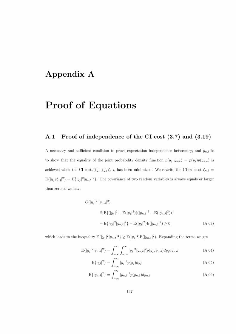
Appendix A
Proof of Equations
A.1 Proof of independence of the CI cost (3.7) and (3.19)
A necessary and sufficient condition to prove expectation independence between yj and yn,δ is
to show that the equality of the joint probability density function p(yj , yn,δ) = p(yj)p(yn,δ) is
achieved when the CI cost,∑
n
∑δ ζn,δ, has been minimized. We rewrite the CI subcost ζn,δ =
E|yjy∗n,δ|2 = E|yj |2|yn,δ|2. The covariance of two random variables is always equals or larger
than zero so we have
C(|yj |2,|yn,δ|2)
, E(|yj |2 − E(|yj |2))(|yn,δ|2 − E(|yn,δ|2))
= E|yj |2|yn,δ|2 − E(|yj |2)E(|yn,δ|2) ≥ 0 (A.63)
which leads to the inequality E|yj |2|yn,δ|2 ≥ E(|yj |2)E(|yn,δ|2). Expanding the terms we get
E|yj |2|yn,δ|2 =
∫ ∞
−∞
∫ ∞
−∞|yj |2|yn,δ|2p(yj , yn,δ)dyjdyn,δ (A.64)
E|yj |2 =
∫ ∞
−∞|yj |2p(yj)dyj (A.65)
E|yn,δ|2 =
∫ ∞
−∞|yn,δ|2p(yn,δ)dyn,δ (A.66)
137

Therefore for the equality to occur which corresponds to the CI subcost being minimized, the
independence between yj and yn,δ must have been achieved giving p(yj , yn,δ) = p(yj)p(yn,δ).
138
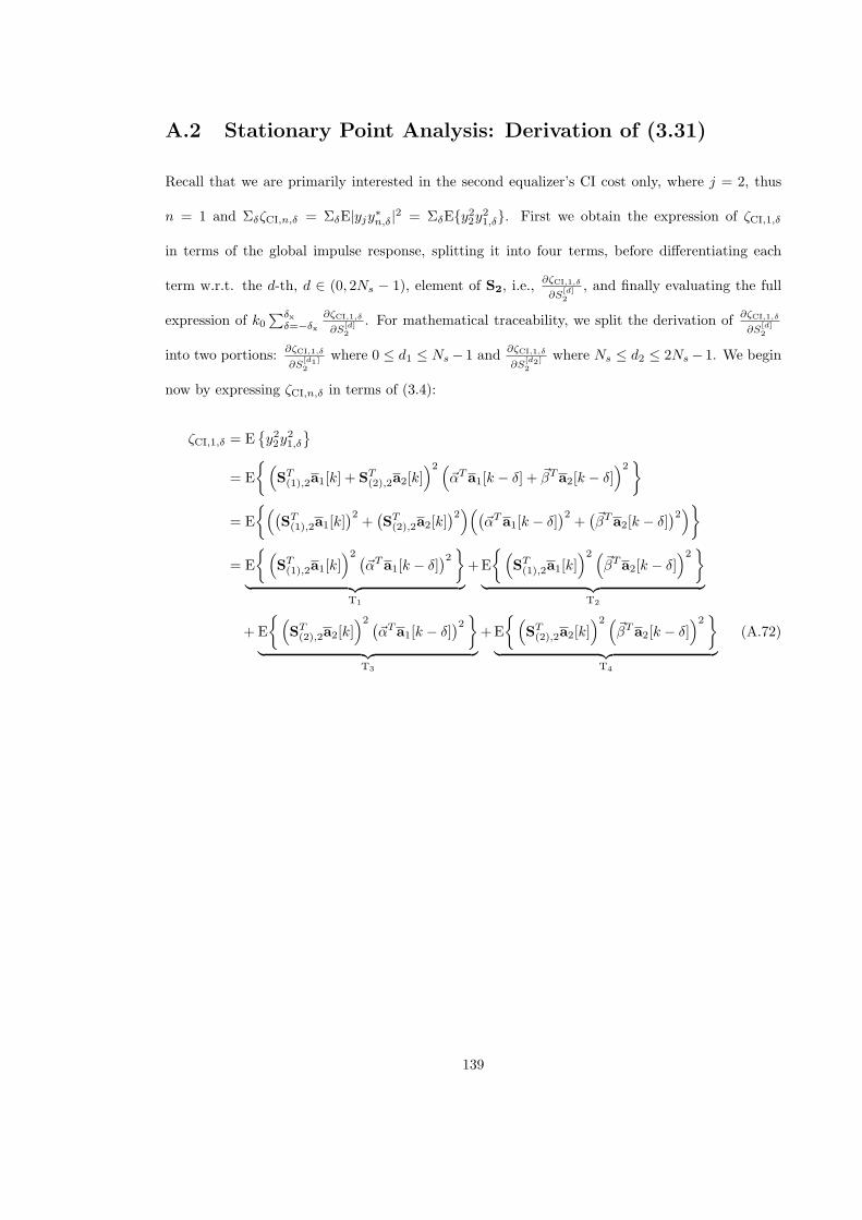
A.2 Stationary Point Analysis: Derivation of (3.31)
Recall that we are primarily interested in the second equalizer’s CI cost only, where j = 2, thus
n = 1 and ΣδζCI,n,δ = ΣδE|yjy∗n,δ|2 = ΣδEy22y21,δ. First we obtain the expression of ζCI,1,δ
in terms of the global impulse response, splitting it into four terms, before differentiating each
term w.r.t. the d-th, d ∈ (0, 2Ns − 1), element of S2, i.e.,∂ζCI,1,δ
∂S[d]2
, and finally evaluating the full
expression of k0∑δx
δ=−δx
∂ζCI,1,δ
∂S[d]2
. For mathematical traceability, we split the derivation of∂ζCI,1,δ
∂S[d]2
into two portions:∂ζCI,1,δ
∂S[d1]2
where 0 ≤ d1 ≤ Ns − 1 and∂ζCI,1,δ
∂S[d2]2
where Ns ≤ d2 ≤ 2Ns − 1. We begin
now by expressing ζCI,n,δ in terms of (3.4):
ζCI,1,δ = Ey22y
21,δ
= E
(ST(1),2a1[k] + ST
(2),2a2[k])2 (
αTa1[k − δ] + βTa2[k − δ])2
= E
((ST(1),2a1[k]
)2+(ST(2),2a2[k]
)2)((αTa1[k − δ]
)2+(βTa2[k − δ]
)2)= E
(ST(1),2a1[k]
)2 (αTa1[k − δ]
)2︸ ︷︷ ︸
T1
+E
(ST(1),2a1[k]
)2 (βTa2[k − δ]
)2︸ ︷︷ ︸
T2
+ E
(ST(2),2a2[k]
)2 (αTa1[k − δ]
)2︸ ︷︷ ︸
T3
+E
(ST(2),2a2[k]
)2 (βTa2[k − δ]
)2︸ ︷︷ ︸
T4
(A.72)
139
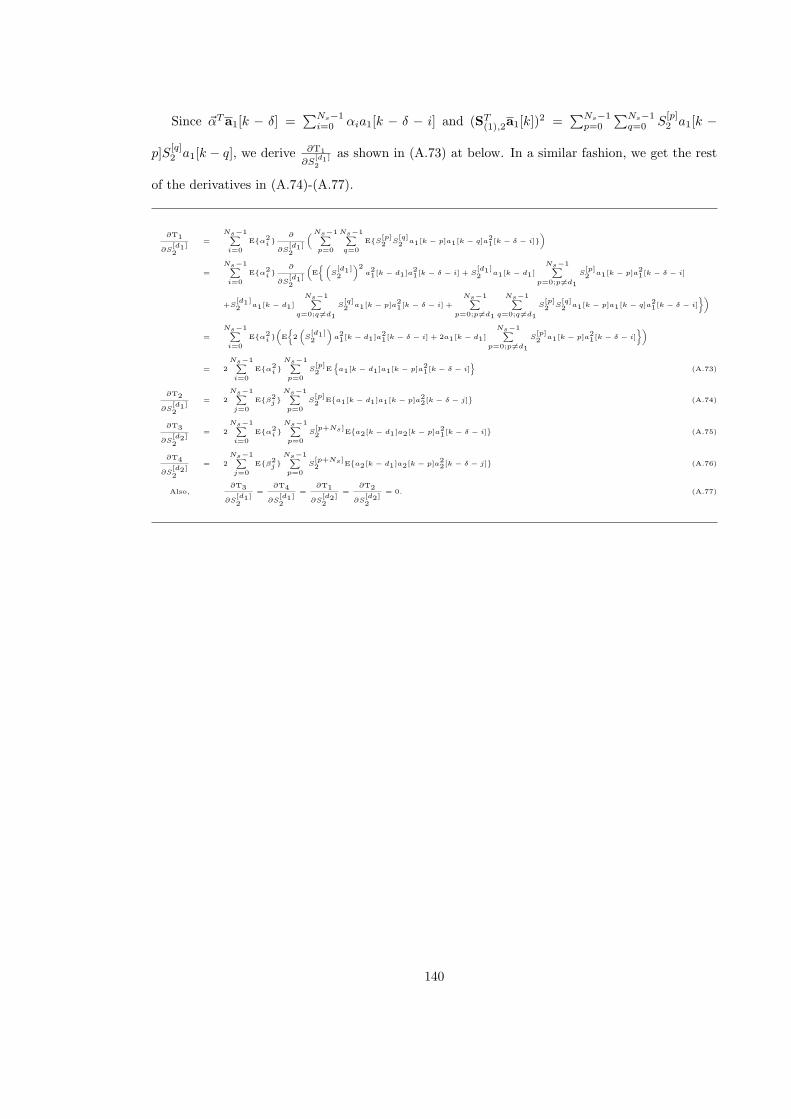
Since αTa1[k − δ] =∑Ns−1
i=0 αia1[k − δ − i] and (ST(1),2a1[k])
2 =∑Ns−1
p=0
∑Ns−1q=0 S
[p]2 a1[k −
p]S[q]2 a1[k − q], we derive ∂T1
∂S[d1]2
as shown in (A.73) at below. In a similar fashion, we get the rest
of the derivatives in (A.74)-(A.77).
∂T1
∂S[d1]2
=
Ns−1∑i=0
Eα2i
∂
∂S[d1]2
(Ns−1∑p=0
Ns−1∑q=0
ES[p]2 S
[q]2 a1[k − p]a1[k − q]a
21[k − δ − i]
)
=
Ns−1∑i=0
Eα2i
∂
∂S[d1]2
(E
(S[d1]2
)2a21[k − d1]a
21[k − δ − i] + S
[d1]2 a1[k − d1]
Ns−1∑p=0;p =d1
S[p]2 a1[k − p]a
21[k − δ − i]
+S[d1]2 a1[k − d1]
Ns−1∑q=0;q =d1
S[q]2 a1[k − p]a
21[k − δ − i] +
Ns−1∑p=0;p =d1
Ns−1∑q=0;q =d1
S[p]2 S
[q]2 a1[k − p]a1[k − q]a
21[k − δ − i]
)
=
Ns−1∑i=0
Eα2i
(E
2
(S[d1]2
)a21[k − d1]a
21[k − δ − i] + 2a1[k − d1]
Ns−1∑p=0;p =d1
S[p]2 a1[k − p]a
21[k − δ − i]
)
= 2
Ns−1∑i=0
Eα2i
Ns−1∑p=0
S[p]2 E
a1[k − d1]a1[k − p]a
21[k − δ − i]
(A.73)
∂T2
∂S[d1]2
= 2
Ns−1∑j=0
Eβ2j
Ns−1∑p=0
S[p]2 E
a1[k − d1]a1[k − p]a
22[k − δ − j]
(A.74)
∂T3
∂S[d2]2
= 2
Ns−1∑i=0
Eα2i
Ns−1∑p=0
S[p+Ns]2 E
a2[k − d1]a2[k − p]a
21[k − δ − i]
(A.75)
∂T4
∂S[d2]2
= 2
Ns−1∑j=0
Eβ2j
Ns−1∑p=0
S[p+Ns]2 E
a2[k − d1]a2[k − p]a
22[k − δ − j]
(A.76)
Also,∂T3
∂S[d1]2
=∂T4
∂S[d1]2
=∂T1
∂S[d2]2
=∂T2
∂S[d2]2
= 0. (A.77)
140
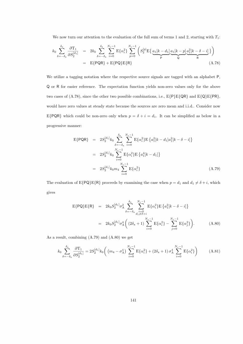
We now turn our attention to the evaluation of the full sum of terms 1 and 2, starting with T1:
k0
δx∑δ=−δx
∂T1
∂S[d1]2
= 2k0
δx∑δ=−δx
Ns−1∑i=0
Eα2i
Ns−1∑p=0
(S[p]2 E
a1[k − d1]︸ ︷︷ ︸
P
a1[k − p]︸ ︷︷ ︸Q
a21[k − δ − i]︸ ︷︷ ︸R
)= EPQR+ EPQER (A.78)
We utilize a tagging notation where the respective source signals are tagged with an alphabet P,
Q or R for easier reference. The expectation function yields non-zero values only for the above
two cases of (A.78), since the other two possible combinations, i.e., EPEQR and EQEPR,
would have zero values at steady state because the sources are zero mean and i.i.d.. Consider now
EPQR which could be non-zero only when p = δ + i = d1. It can be simplified as below in a
progressive manner:
EPQR = 2S[d1]2 k0
δx∑δ=−δx
Ns−1∑i=0
Eα2i E
a21[k − d1]a
21[k − δ − i]
= 2S
[d1]2 k0
Ns−1∑i=0
Eα2i E
a41[k − d1]
= 2S
[d1]2 k0m4
Ns−1∑i=0
Eα2i (A.79)
The evaluation of EPQER proceeds by examining the case when p = d1 and d1 = δ+ i, which
gives
EPQER = 2k0S[d1]2 σ2
A
δx∑δ=−δx
Ns−1∑i=0
d1 =δ+i
Eα2i E
a21[k − δ − i]
= 2k0S[d1]2 σ4
A
((2δx + 1)
Ns−1∑i=0
Eα2i −
Ns−1∑j=0
Eα2j). (A.80)
As a result, combining (A.79) and (A.80) we get
k0
δx∑δ=−δx
∂T1
∂S[d1]2
= 2S[d1]2 k0
((m4 − σ4
A
)Ns−1∑i=0
Eα2i + (2δx + 1)σ4
A
Ns−1∑i=0
Eα2i )
(A.81)
141
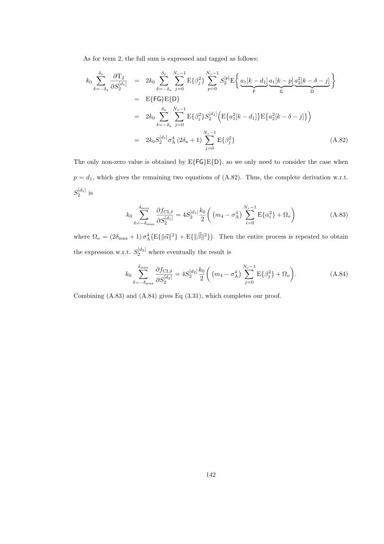
As for term 2, the full sum is expressed and tagged as follows:
k0
δx∑δ=−δx
∂T2
∂S[d1]2
= 2k0
δx∑δ=−δx
Ns−1∑j=0
Eβ2j
Ns−1∑p=0
S[p]2 E
a1[k − d1]︸ ︷︷ ︸
F
a1[k − p]︸ ︷︷ ︸G
a22[k − δ − j]︸ ︷︷ ︸D
= EFGED
= 2k0
δx∑δ=−δx
Ns−1∑j=0
Eβ2j S
[d1]2
(Ea21[k − d1]
Ea22[k − δ − j]
)
= 2k0S[d1]2 σ4
A (2δx + 1)
Ns−1∑j=0
Eβ2j (A.82)
The only non-zero value is obtained by EFGED, so we only need to consider the case when
p = d1, which gives the remaining two equations of (A.82). Thus, the complete derivation w.r.t.
S[d1]2 is
k0
δmax∑δ=−δmax
∂fCI,δ
∂S[d1]2
= 4S[d1]2
k02
((m4 − σ4
A
)Ns−1∑i=0
Eα2i +Ωo
)(A.83)
where Ωo = (2δmax + 1)σ4A
(E∥α∥2 + E∥β∥2
). Then the entire process is repeated to obtain
the expression w.r.t. S[d2]2 where eventually the result is
k0
δmax∑δ=−δmax
∂fCI,δ
∂S[d2]2
= 4S[d2]2
k02
((m4 − σ4
A
)Ns−1∑j=0
Eβ2j +Ωo
). (A.84)
Combining (A.83) and (A.84) gives Eq (3.31), which completes our proof.
142
References
[1] S. Haykin, Unsupervised Adaptive Filtering, Volumne 2: Blind Deconvolution. John Wiley
and Sons Inc., 2000.
[2] A. Touzni, I. Fijalkow, M. G. Larimore, and J. R. Treichler, “A globally convergent approach
for blind MIMO adaptive deconvolution,” IEEE Trans. Signal Processing, vol. 49, pp. 1166–
1178, Jun 2001.
[3] World Health Organization, “Factsheets: Noncommunicable diseases.” http://www.who.
int/mediacentre/factsheets/fs355/en/, 2013. [Online accessed 19-Sep-2014].
[4] R. Dilmaghani, H. Bobarshad, and M. Ghavami, “Wireless Sensor Networks for Monitoring
Physiological Signals of Multiple Patients,” IEEE Transactions on Biomedical Circuits and
Systems, pp. 347–356, 2011.
[5] D. Oletic, B. Arsenali, and V. Bilas, “Low-Power Wearable Respiratory Sound Sensing,”
Open Access Journal Sensors, pp. 6535–6566, 2014.
[6] D. C. Klonoff, “The Benefits of Implanted Glucose Sensors,” Journal Diabetes Science Tech-
nology, vol. 1, no. 6, p. 797800, 2007.
[7] R. Sobot, “Implantable RF telemetry for cardiac monitoring in the murine heart: a tutorial
review,” EURASIP Journal on Embedded Systems, vol. 1, 2013.
143
[8] A. Khaleghi, R. Chavez-Santiago, and I. Balasingham, “Ultra-wideband pulse-based data
communications for medical implants,” IET Communications Journal, vol. 4, pp. 1889–1897,
2010.
[9] K. S. Kwak, S. Ullah, and N. Ullah, “An overview of IEEE 802.15.6 standard,” 3rd Inter-
national Symposium on Applied Sciences in Biomedical and Communication Technologies
(ISABEL), vol. 2, pp. 1–6, Mar 2012.
[10] “IEEE Standard for Local and Metropolitan Area Networks - Part 15.6: Wireless Body Area
Networks. IEEE STD 802.15.6-2012,” IEEE Computer Society, vol. 2, Mar 2012.
[11] R. Chvez-Santiago and K. Sayrafian-Pour and A. Khaleghi et al, “Propagation Models for
IEEE 802.15.6 Standardization of Implant Communication in Body Area Networks,” IEEE
Communications Magazine, pp. 80–87, Aug 2013.
[12] T. Akin, K. Najafi, and R. M. Bradley, “A wireless implantable multichannel digital neural
recording system for a micromachined sieve electrode,” IEEE J. Solid-State Circuits, vol. 33,
no. 1, pp. 109–118, 1998.
[13] P. R. Troyk and M. A. K. Schwan, “Closed-loop class E transcutaneous power and data link
for microimplants,” IEEE Trans. Biomed. Eng., vol. 39, no. 6, p. 589599, 1998.
[14] M. Ghovanloo and K. Najafi, “A wide-band frequency-shift keying wireless link for in-
ductively powered biomedical implants,” IEEE Trans. Circuits Syst. I, vol. 51, no. 12,
p. 23742383, 2004.
[15] P. Mohseni and K. Najafi, “Wireless multi-channel biopotential recording using an integrated
FM telemetry circuit,” IEEE Trans. Neural. Syst. Rehabil. Eng, vol. 13, p. 263271, 2005.
[16] R. Bashirullah, “Wireless Implants,” IEEE Microwave Magazine, vol. 11, no. 7, pp. S14–S23,
2010.
144
[17] H. Tsuji and J. Zheng and K. Mostafa, “Experiments in radio location estimation using an
airbone array,” IEEE Sensor Array and Multichannel Signal Processing Workshop, pp. 189–
193, July 2008.
[18] H. Artes, D. Seethaler, and F. Hlawatsch, “Efficient detection algorithms for MIMO channels:
A geometrical approach to approximate ML detection,” IEEE Trans. Signal Processing,
Special Issue on MIMO Communications Systems, vol. 51, pp. 2808–2820, Nov 2003.
[19] M. Chouayakh, A. Knopp, and B. Lankl, “Low-effort near maximum likelihood MIMO de-
tection with optimum hardware resource exploitation,” Electronics Letters, vol. 43, pp. 1104–
1106, Sep 2007.
[20] O. Macchi, Adaptive processing. The LMS Approach with Applications in Transmission. New
York: Wiley, 1995.
[21] D. N. Godard, “Self-recovering equalization and carrier tracking in two dimensional data
communication system,” IEEE Trans. Commun., vol. 28, pp. 1867–1875, Nov 1980.
[22] Y. Sato, “A method of self-recovering equalization for multi-level amplitude-modulations
systems,” IEEE Trans. Commun., pp. 679–682, Jun 1975.
[23] J. Yang, J.-J. Werner, and G. A. Dumont, “The multimodulus blind equalization and its
generalized algorithms,” IEEE Journal on selected areas in communications, vol. 20, pp. 997–
1015, Jun 2002.
[24] K. N. Oh and Y. O. Chin, “New blind equalization techniques based on constant modulus
algorithm,” Proc. 1995 IEEE Global Telecommunications Conf., Singapore, pp. 865–869, Nov
14-16 1995.
[25] O. Shalvi and E. Weinstein, “New criteria for blind deconvolution of nonminimum phase
systems (channels),” IEEE Trans. Information Theory, vol. 36, Mar 1990.
145
[26] A. Hyvarinen, J. Karhunen, and E. Oja, Independent Component Analysis. John Wiley and
Sons, 1st ed., 2001.
[27] P. Comon, “Independent component analysis, a new concept?,” Elsevier Sigal Processing,
vol. 36, pp. 287–314, Apr 1994.
[28] C. B. Papadias, “Globally convergent blind source separation based on a multiuser kurtosis
maximization criterion,” IEEE Trans. Signal Processing, vol. 48, pp. 3508–3519, Dec 2000.
[29] M. Phegade, P. Mukherji, and U. S. Sutar, “Hybrid ICA algorithm for ECG analysis,”
International Conference on Hybrid Intelligent Systems, vol. 35, pp. 478–483, Mar 2012.
[30] G. R. Naik and D. K. Kumar, “An Overview of Independent Component Analysis and Its
Applications,” Informatica, vol. 35, Mar 2011.
[31] C. B. Papadias and A. J. Paulraj, “A constant modulus algorithm for multiuser signal sepa-
ration inpresence of delay spread using antenna arrays,” IEEE Signal Processing Lett., vol. 2,
pp. 178–181, Jun 1997.
[32] P. Sansrimahachai, D. B. Ward, and A. G. Constantinides, “Blind source separation for
BLAST,” Conf. Digital Signal Processing, vol. 1, pp. 139–142, July 2002.
[33] A. Ikhlef and D. L. Guennec, “Blind recovery of MIMO QAM signals: a criterion with
its convergence analysis,” Proceedings of the 14th European Signal Processing Conference
(EUSIPCO’06), no. 1, 2006.
[34] A. Ikhlef and D. L. Guennec, “A simplified constant modulus algorithm for blind recovery
of MIMO QAM and PSK signals: a criterion with convergence analysis,” EURASIP Journal
on Wireless Communications and Networking 2007, vol. 15, 2007.
[35] R. Gooch and J. Lundell, “The cm array: An adaptive beamformer for constant modulus
signals,” Proc. IEEE Acoustics, Speech, and Signal Process. (ICASSP), pp. 2523–2526, 1986.
146
[36] Y. Li and K. J. R. Liu, “Adaptive blind source separation and equalization for multiple-
input/multiple-output systems,” IEEE Trans. Information Theory, vol. 44, pp. 2864–2876,
Nov 1998.
[37] C. Meng, J. Tuqan, and Z. Ding, “A Quadratic Programming Approach to Blind Equalization
and Signal Separation,” IEEE Trans. Signal Processing, vol. 57, pp. 3196–3203, Dec 2009.
[38] H. D. Han and Z. Ding, “Steepest descent algorithm implementation for multichannel blind
signal recovery,” IET Communications Journal, vol. 6, pp. 2232–2244, Dec 2012.
[39] M. Castella, S. Rhioui, E. Moreau, and J. Pesquet, “Quadratic Higher-Order Criteria for
Iterative Blind Separation of a MIMO Convolutive Mixture of Sources,” IEEE Trans. Signal
Processing, vol. 55, Jan 2007.
[40] M. Kawamoto, Y. Inouye, K. Kohno, and T. Maeda, “An Eigenvector Algorithm with Ref-
erence Signals Using a Deflation Approach for Blind Deconvolution,” 7th International Con-
ference, ICA 2007, 2007.
[41] J. Via, I. Santamaria, and J. Perez, “Deterministic CCA-Based Algorithms for Blind Equal-
ization of FIR-MIMO Channels,” IEEE Trans. Signal Processing, vol. 55, pp. 3867–3878,
July 2007.
[42] L. Castedo, C. J. Escudero, and A. Dapena, “A blind signal separation method for multiuser
communications,” IEEE Trans. Signal Process., vol. 45, pp. 1343–1348, May 1997.
[43] Y. Luo, J. A. Chambers, and S. Lambotharan, “Global convergence and mixing parameter se-
lection in the cross-correlation constant modulus algorithm for the multi-user environment,”
IEE Proc. Visual Image Signal Proceessing, vol. 148, pp. 9–20, Feb 2001.
[44] S. Li, T. S. Qiu, and S. F. Zhang, “Space-time blind equalisation in impulsive noise,” IET
Signal Process., vol. 3, no. 6, pp. 445–458, 2009.
147
[45] S. Li, T. Qui, and D. Zha, “Adaptive blind equalization for MIMO systems under alpha-stable
noise environment,” IEEE Commun. Letter, vol. 13, pp. 609–611, Aug 2009.
[46] A. Vgenis, C. S. Petrou, C. B. Papadias, I. Roudas, and L. Raptis, “Nonsingular constant
modulus equalizer for PDM-QPSK coherent optical receivers,” IEEE Photnics Technology
Letters, vol. 22, pp. 45–47, Jan 2010.
[47] S. Li, “Space-Time Blind Equalization under alpha-Stable Noise Environment,” Wireless
Communications, Networking and Mobile Computing, pp. 1–4, Sept 2009.
[48] M. Silva, M. Miranda, and A N Licciardi Jr, “A robust algorithm for space-time equalization,”
Proc. ICASSP 04, pp. 857–860, 2004.
[49] A. M. Nassar and E. W. E. Nahal, “Blind equalization technique for cross correlation constant
modulus algorithm,” WSEAS Transaction on Signal Process., vol. 6, no. 2, pp. 23–32, 2010.
[50] Y. Luo and J. A. Chambers, “Steady state mean-square error analysis of the cross-correlation
and constant modulus algorithm in a mimo convolutive system,” Proc. 2002 IEE Vision,
Image and Signal Processing, vol. 149, pp. 196–203, 2002.
[51] Y. Luo, S. Lambotharan, and J. A. Chambers, “Global convergence and mixing parameter
selection in the cross correlation constant modulus algorithm for the multi-user environment,”
Proc. IEE Vision, Image and Signal Processing, vol. 148, pp. 9–20, 2001.
[52] Y. Luo and J. A. Chambers, “Bounds for the mixing parameter within the cc-cma algorithm
applied in non ideal multiuser environments,” Proc. 2001 IEEE Acoustics, Speech, and Signal
Process. (ICASSP), vol. 4, pp. 2173–2176, 2001.
[53] S. Lambotharan and J. A. Chambers, “On the surface characteristics of a mixed constant
modulus and cross-correlation for the blind equalisation of a mimo channel,” Elsevier Signal
Processing, vol. 72, no. 2, pp. 209–216, 1999.
148
[54] J. Mai and A.H. Sayed, “A feedback approach to the steady-state performance of fractionally
spaced blind adaptive equalizers,” IEEE Trans. Signal Process., vol. 48, no. 1, pp. 80–91,
2000.
[55] Centers for Disease Control and Prevention, “Chronic Diseases and Health Promotion.”
http://www.cdc.gov/chronicdisease/overview/, 2014. [Online accessed 19-Sep-2014].
[56] W. Chodzko-Zajko, D. Proctor, , M. F. Singh, C. Minson, C. Nigg, G. Salem, and J. Skinner,
“American College of Sports Medicine Position Stand. Exercise and Physical Activity for
Older Adults,” Med. Sci. Sport. Exerc, vol. 41, pp. 1510–1530, 2009.
[57] L. Allet, R. H. Knols, K. Shirato, and E. D. de Bruin, “Wearable Systems for Monitoring
Mobility-Related Activities in Chronic Disease: A Systematic Review,” Open Access Journal
Sensors, pp. 9026–9052, 2010.
[58] L. Wang, G. Yang, J. Huang, J. Zhang, L. Yu, and Z. Nie, “A wireless biomedical signal in-
terface system-on-chip for body sensor networks,” IEEE Transaction on Biomedical Circuits
and Systems, vol. 4, pp. 112–117, 2010.
[59] S. Patel, H. Park, , P. Bonato, L. Chan, and M. Rodgers, “A review of wearable sensors and
systems with application in rehabilitation,” Journal of NeuroEngineering and Rehabilitation,
vol. 9, no. 21, 2012.
[60] S. Gulley, E. Rasch, and L. Chan, “If we build it, who will come? Working-age adults with
chronic health care needs and the medical home,” Medical Care, vol. 49, no. 2, pp. 149–155,
2011.
[61] P. Bonato, “Wearable sensors and systems. From enabling technology to clinical applica-
tions,” IEEE Engineering in Medicine and Biology Magazine, vol. 29, pp. 25–36, 2010.
[62] N. Oliver and F. Flores-Mangas, “HealthGear: Automatic Sleep Apnea Detection and Mon-
itoring with a Mobile Phone,” Journal Of Communications, vol. 2, Mar 2007.
149
[63] P. Corbishley and Rodriguez-Villegas, “Breathing detection: towards a miniaturized, wear-
able, battery-operated monitoring system,” IEEE Transaction on Biomedical Engineering,
vol. 55, pp. 196–204, 2008.
[64] W. Haiying, Z. Huiru, and J. A. JC, “Monitoring and analysis of sleep pattern for people
with early dementia,” IEEE International Conference on Bioinformatics and Biomedicine
Workshops (BIBMW), pp. 405–410, 2010.
[65] J. Jimison, M. Pavel, J. Pavel, and J. McKanna, “Home monitoring of computer interactions
for the early detection of dementia,” 26th Annual International Conference of the IEEE
Engineering in Medicine and Biology Society, pp. 4533–4536, 2004.
[66] J. Zhang, P. Orlik, Z. Sahinoglu, A. Molisch, and P. Kinney, “UWB systems for wireless
sensor networks,” Proceedings of the IEEE, vol. 97, pp. 313–331, 2009.
[67] M. Hernandez and R. Kohno, “UWB systems for body area networks in IEEE 802.15. 6,”
IEEE International Conference on Ultra-Wideband (ICUWB), pp. 235–239, 2011.
[68] M. H. V. Niemel and J. Iinatti, “IEEE 802.15. 4a UWB Receivers in medical applications,”
International Journal of Ultra Wideband Communications and Systems, vol. 2, pp. 73–82,
2011.
[69] B. Z. W. Rhee, N. Xu and Z. Wang, “Low power, non invasive UWB systems for WBAN
and biomedical applications,” International Conference on Information and Communication
Technology Convergence (ICTC), vol. 2, pp. 35–40, 2010.
[70] M. H. H. Viittala, B. N. Nahar and J. Iinatti, “Medical applications adapting ultra wideband:
a system study,” International Journal of Ultra Wideband Communications and Systems,
vol. 1, pp. 237–247, 2010.
150
[71] M. Hernandez and R. Kohno, “Ultra low power UWB transceiver design for body area net-
works,” 2nd International Symposium on Applied Sciences in Biomedical and Communication
Technologies (ISABEL), vol. 1, pp. 1–4, 2009.
[72] N. Kernen, M. Srestniemi, and J. Partala, “IEEE802.15.6 based Multi-Accelerometer WBAN
System for Monitoring Parkinson’s Disease,” 35th Annual International Conference of the
IEEE EMBS, pp. 1656–1659, 2013.
[73] A. Darwish and A. E. Hassanien, “Wearable and Implantable Wireless Sensor Network So-
lutions for Healthcare Monitoring,” Sensors, vol. 11, no. 6, p. 55615595., 2011.
[74] Masihpour Mehrnoush, Cooperative communication in near field magnetic induction commu-
nication systems. PhD Thesis, University of Technology, Sydney, 2012.
[75] O. Brand, “Microsensor integration into systems-on-chip,” IEEE Engineering in Medicine
and Biology Magazine, vol. 94, pp. 1160–1176, 2006.
[76] Vemund Svanes Bertelsen, Communication System for a Medical Implant. Msc Thesis, Un-
vierstiy of Oslo, 2004.
[77] Eliza Strickland, “Medtronic Wants to Implant Sensors in Everyone, IEEE
Spectrum.” http://spectrum.ieee.org/tech-talk/biomedical/devices/
medtronic-wants-to-implant-sensors-in-everyone, 2014. [Online accessed 19-
Sep-2014].
[78] F. M. Merchant, G. W. Dec, and J. P. Singh, “Implantable Sensors for Heart Failure,” Cir-
culation: Arrhythmia and Electrophysiology, American Heart Association, p. 657667, 2010.
[79] “World Cancer Report 2014,” World Health Organization, 2014.
[80] A. C. Society, “Global cancer facts and figures.” http://www.cancer.org/acs/groups/
content/@epidemiologysurveilance/documents/document/acspc-027766.pdf, 2011.
[Online accessed 19-Sep-2014].
151
[81] World Health Organization, “Factsheets: Cancer.” http://www.who.int/mediacentre/
factsheets/fs297/en/, 2014. [Online accessed 19-Sep-2014].
[82] K. Choudhari et al, “Nitric oxide and cancer: a review,” World Journal of Surgical Oncology,
2013.
[83] Medical News Today, “Implantable sensor may monitor cancer and diabetes.” http://www.
medicalnewstoday.com/articles/268347.php, 2013. [Online accessed 19-Sep-2014].
[84] G. Ciuti, A. Menciassi, and P. Dario, “Capsule Endoscopy: From Current Achievements to
Open Challenges,” IEEE Review in Biomedical Engineering, vol. 4, pp. 59–72, 2012.
[85] Y. Gu, X. Xie, Z. Wang, and G. Li, “A new globularity capsule endoscopy system with
multi-camera,” IEEE Biomedical Circuits and Systems Conference, pp. 289–292, 2009.
[86] L. Dong and Y. Wu, “A Wireless Narrowband Imaging Chip for Capsule Endoscope,” IEEE
Transactions On Biomedical Circuits Aand Systems, vol. 4, no. 6, pp. 462–468, 2010.
[87] E. Jovanov and A. Milenkovic, “Body area networks for ubiquitous healthcare applications:
opportunities and challenges,” Journal of Medical Systems, vol. 35, pp. 1245–1254, 2011.
[88] Anders J. Johansson, Wireless Communication with Medical Implants: Antennas and Prop-
agation. PhD Thesis, Lund University, Sweden, 2004.
[89] K. Y. Yazdandoost and R. Kohno, “Wireless Communications for Body Implanted Medical
Device,” Microwave Conference, 2007.
[90] J. Wang and Q. Wang, “Channel Modeling and BER Performance of an Implant UWB Body
Area Link,” Proc. 2nd Intl. Symp. Applied Sciences in Biomedical and Commun. Technolo-
gies, pp. 24–27, 2009.
[91] A. Khaleghi, R. Chvez-Santiago, and I. Balasingham, “An Improved Ultra Wideband Chan-
nel Model Including the Frequency-Dependent Attenuation for In-Body Communications,”
Proc. 34th Annual Intl. Conf. IEEE Eng. in Medicine and Biology Society, p. 16311634, 2012.
152
[92] G. Wunder, R. F. H. Fischer, H. Boche, S. Litsyn, and J.-S. No, “The PAPR Problem in
OFDM Transmission: New Directions for a Long-Lasting Problem,” IEEE Signal Processing
Magazine, pp. 130–144, Nov 2013.
[93] J.-H. Wen, G.-R. Lee, C.-C. Kung, and C.-Y. Yang, “Coding Schemes Applied to Peak-to-
Average Power Ratio (PAPR) Reduction in OFDM Systems,” International Wireless Com-
munications and Mobile Computing Conference, pp. 807–812, Aug 2008.
[94] Z. Zhang, K. Long, M. Zhao, and Y. Liu, “Joint Frame Synchronization and Frequency Offset
Estimation in OFDM Systems,” IEEE Transaction On Broadcasting, vol. 51, pp. 389–394,
Sept 2005.
[95] M. H. Akbari, M. Ahmadian, and S. Salari, “Joint Frame and Frequency Synchronization
for MIMO OFDM Systems with ZCZ Sequences,” 3rd IEEE/IFIP International Conference
in Central Asia on Internet, pp. 1–5, 2007.
[96] Z. Ye, C. Duan, P. V. Orlik, J. Zhang, and A. A. Abouzeid, “A Synchronization Design for
UWB-Based Wireless Multimedia Systems,” IEEE Transaction On Broadcasting, pp. 211–
225, 2010.
[97] Y. Mostofi, “Analysis of the effect of timing synchronization errors on pilot-aided ofdm
systems,” IEEE Conference on Signals, Systems and Computers, vol. 1, pp. 638–642, Nov
2003.
[98] T. Haritha, S. SriGown, and D. E. Rani, “Frequency offset estimation in coherent ofdm
systems using different fading channels,” ARPN Journal of Engineering and Applied Science,
vol. 7, pp. 691–695, June 2013.
[99] G. Tatsis, C. Votis, V. Raptis, V. Christofilakis, and P. Kostarakis, “A/D Restrictions (Er-
rors) in Ultra-Wideband Impulse Radios ,” Int. J. Communications Network and System
Sciences, vol. 3, pp. 425–429, 2010.
153
[100] R. Akbar and E. Radoi, “An overview of synchronization algorithms for IR-UWB systems,”
International Conference on Computing, Networking and Communications (ICNC), pp. 573–
577, 2012.
[101] H. Aubert, “RFID Technology for Human Implant Devices ,” Special Issue on Nanoscience
and nanotechnologies: hopes and concerns, vol. 12, no. 7, pp. 675–683, 2011.
[102] M. Sun, S. A. Hackworth, Z. Tang, G. Gilbert, S. Cardin, and R. J. Sclabassi, “How to
pass information and deliver energy to a network of implantable devices within the human
body,” Proc. IEEE Conf. on Engineering in Medicine and Biology Society (EMBS 2007),
pp. 5286–5289, 2007.
[103] Z. Nie, T. Leng, W. Wang, F. Guan, and L. Wang, “Experimental Characterization of human
body communication in shield chamber,” 2012 IEEE-EMBS International Conference on
Biomedical and Health Informatics (BHI), pp. 759–762, 2012.
[104] H. Higgins, “Body Implant Communication - Is It A Reality?,” IET Seminar on Antennas
and Propagation for Body-Centric Wireless Communications, pp. 33–36, 2007.
[105] Y. Yu, Blind Identification of Possibly Under-determined Convolutive MIMO Systems. PhD
Thesis, Drexel University, July 2007.
[106] C. Y. Chi, C. C. Feng, C. H. Chen, and C. Y. Chen, Blind Equalization and System Identifica-
tion: Batch Processing Algorithms, Performance and Applications. Springer-Verlag London
Limited, 1st ed., 2006.
[107] R. T. Causey, Blind Multiuser Detection Based on Second-Order Statistics. PhD Thesis,
Georgia Institutue of Technology, 1999.
[108] R. W. Lucky, “Techniques for adaptive equalization of digital communciation systems,” Bell
System Tehnical Journal, vol. 45, Feb 1966.
154
[109] Y. Li and Z. Ding, “Convergence analysis of finite length blind adaptive equalizers,” IEEE
Trans. Signal Processing, vol. 43, pp. 2120–2129, Sep 1995.
[110] Y. Li and Z. Ding, “Static and dynamic convergence behavior of adaptive blind equalizers,”
IEEE Trans. Signal Processing, vol. 44, pp. 2736–2745, Nov 1996.
[111] Y. Li, K. J. R. Liu, and Z. Ding, “Length and cost dependent local minima of blind channel
equalizers,” IEEE Trans. Signal Processing, vol. 44, pp. 2726–2735, Nov 1996.
[112] S. Bellini, “Bussgang techniques for blind equalization,” GLOBECOM, pp. 1634–1640, 1986.
[113] S. M. Kay, Fundamentals of Statistical Signal Processing, Volume I: Estimation Theory.
Prentice Hall, 1st ed., 1993.
[114] S. Haykin, Blind Deconvolution. Prentice Hall Information and System Sciences Series, 1994.
[115] S. Haykin, Adaptive Filter Theory. Prentice Hall Information and System Sciences Series,
3 ed., 1996.
[116] A. H. Sayed, Adaptive Filters. John Wiley and Sons, 2008.
[117] J. G. Proakis, Digital Communications. McGraw-Hill International Editions, 2 ed., 1989.
[118] R. A. Kennedy, B. Anderson, Z. Ding, and C. R. Johnson, Jr., “Local stable minima of the
Sato recursive identification scheme,” Decision and Control, 1990., Proceedings of the 29th
IEEE Conference on, vol. 6, pp. 3194–3199, Dec 1990.
[119] J. R. Treichler and B. G. Agee, “A new approach to multipath correction of constant modulus
signals,” IEEE Trans. Signal Processing, vol. 31, pp. 349–372, Apr 1983.
[120] Z. Ding, R. A. Kennedy, C. R. Johnson, Jr., and B. D. O. Anderson, “Ill-convegence of
Godard blind equalizers in data communication systems,” IEEE Trans. Commun., vol. 39,
pp. 1313–1326, Sep 1991.
155
[121] C. R. Johnson, Jr. et al., “Blind equalization using the constant modulus criterion: A review,”
Proc. IEEE, vol. 86, pp. 1927–1950, Oct 1998.
[122] M. G. Larimore and J. R. Treichler, “Convergence behavior of the Constant Modulus Algo-
rithm,” ICASSP (Boston), pp. 13–16, Apr 1983.
[123] I. Fijalkow, C. Manlove, and C. R. Johnson, Jr., “Adaptive fractionally spaced blind CMA
equalization: Excess MSE,” IEEE Trans. Signal Processing, vol. 46, pp. 227–231, Jan 1998.
[124] G. Picchi and G. Prati, “Blind equalization and carrier recovery using a “Stop-and-Go”
decision-directed algorithm,” IEEE Trans. Commun., vol. COM-35, pp. 877–887, Sep 1987.
[125] A. Benveniste and M. Goursat, “Blind equalizers,” IEEE Trans. Commun., vol. COM-32,
pp. 871–883, Aug 1984.
[126] W. G. Lim, T. D. Abhayapala, and R. A. Kennedy, “Reliability based soft transition tech-
nique for dual-mode blind equalizers,” IEEE International Conference on Communications,
Paris, vol. 5, pp. 2631–2635, Jun 2004.
[127] W. G. Lim, “New soft transition dual mode type algorithms for blind equalization,” IEEE
Wireless Communications and Networking Conference (WCNC 2007), Hong Kong, pp. 504–
508, Mar 11–15 2007.
[128] N. Delfosse and P. Loubaton, “Adaptive separation of independent sources: a deflation
approach,” ICASSP, vol. 4, 1994.
[129] S. Icart, P. Comon, and L. Rota, “Blind paraunitary equalization,” Signal Processing (Else-
vier), pp. 283–290, 2009.
[130] R. Bronson, Schaum’s Theory and Problems of Matrix Operations. McGraw Hill, 1st ed.,
1989.
156

[131] M. Silva and M. Miranda, “Tracking analysis of some space-time blind equalization algo-
rithms,” Proc. 2005 IEEE/SP 13th Workshop on Statistical Signal Processing, pp. 167–172,
2005.
[132] W. G. Lim, “Automatic phase recovery properties of blind adaptive equalization algorithms,”
IEEE 8th Malaysia International Conference on Communications, Penang, May 14–17 2007.
157

List of Publications
• Zhi-Hou Lee and Wee Gin Lim,“Multi-user multimodulus algorithm in blind source sep-
aration and equalization for MIMO systems, IEEE Malaysia International Conference on
Communications (MICC), Kuala Lumpur, 2009, pp 234-237.
• Zhi-Hou Lee and Wee Gin Lim,“Hybrid methods in MIMO blind equalization and source
separation, IEEE Symposium on Industrial Electronic and Applications (ISIEA), 2010, pp
5-9.
• Zhi-Hou Lee, and David Wee-Gin Lim, “Energy normalized cross-correlation constant modu-
lus algorithm in a MIMO convolutive system, IEEE 10th International Conference on Signal
Processing (ICSP), 24-28 Oct 2010, pp. 1445-1448.
158