Lee Dong-yun¹, Chulan Kwon², Hyuk Kyu Pak¹ Department of physics, Pusan National University,...

Lee Dong-yun¹, Chulan Kwon², Hyuk Kyu Pak¹

Department of physics, Pusan National University, Korea¹

Department of physics, Myongji University, Korea²

Nonequilibrium Statistical Physics of Complex Systems, KIAS, July 8, 2014

Experimental Verification of the Fluctuation Theorem in Expansion/Compression Processes of a Single-Particle Gas

BIO-SOFT MATTER PHYSICS LAB

Ph. D studnt: Dong Yun Lee

Collaborator: Chulan Kwon

Outline

Introduction

Experiment

Results

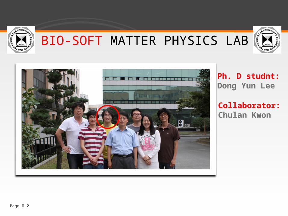
Crooks Fluctuation Theorem (CFT, G. E. Crooks 1998)

CFT has drawn a lot of attention because of its usefulness in experiment. This theorem makes it possible to experimentally measure the free energy difference of the system during a non-equilibrium process.

)](exp[)(

)(FW

WP

WP

b

f

)( WPb )(WPf

F

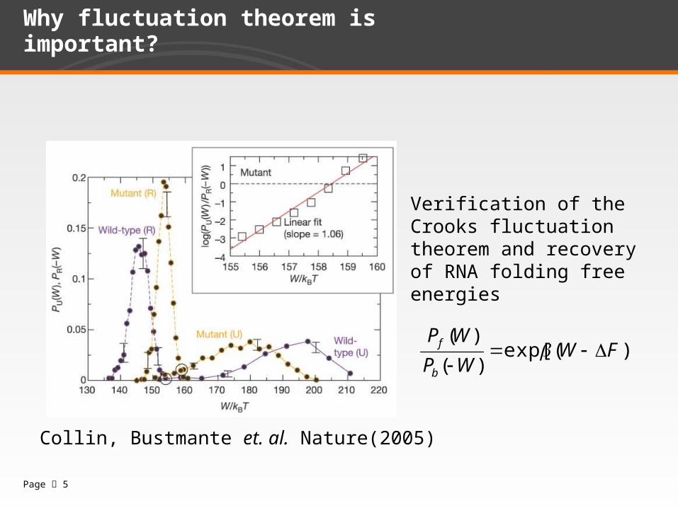
Why fluctuation theorem is important?

Verification of the Crooks fluctuation theorem and recovery of RNA folding free energies

Collin, Bustmante et. al. Nature(2005)

)](exp[)(

)(FW

WP

WP

b

f

Idea

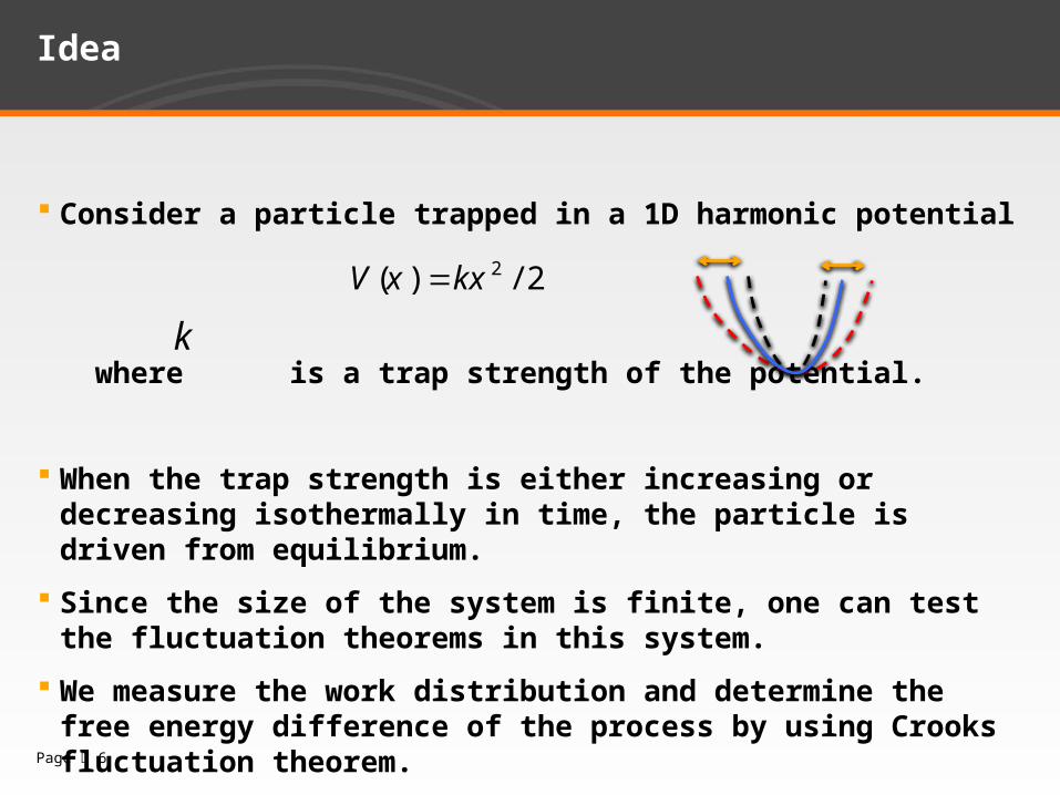
Consider a particle trapped in a 1D harmonic potential

where is a trap strength of the potential.

When the trap strength is either increasing or decreasing isothermally in time, the particle is driven from equilibrium.

Since the size of the system is finite, one can test the fluctuation theorems in this system.

We measure the work distribution and determine the free energy difference of the process by using Crooks fluctuation theorem.

2/)( 2kxxV

k

Free Energy Difference of the System

Harmonic oscillator (in 1D) - Hamiltonian is given by

- Partition function is

- Free energy difference between two equilibrium states at the same temperature is

- Forward process : ,

Backward process: - During these processes:

mkhdxdppxHZ /,/1/),(exp

22

2

1

2),( kx

m

ppxH

i

fif k

kZZF ln2/1)ln()ln(

)0(0 SFkk if

)0(0 SFkk if

fi kk ,

forward

backward

𝑈 ≡ ⟨ 𝐸 ⟩=𝑘𝐵𝑇

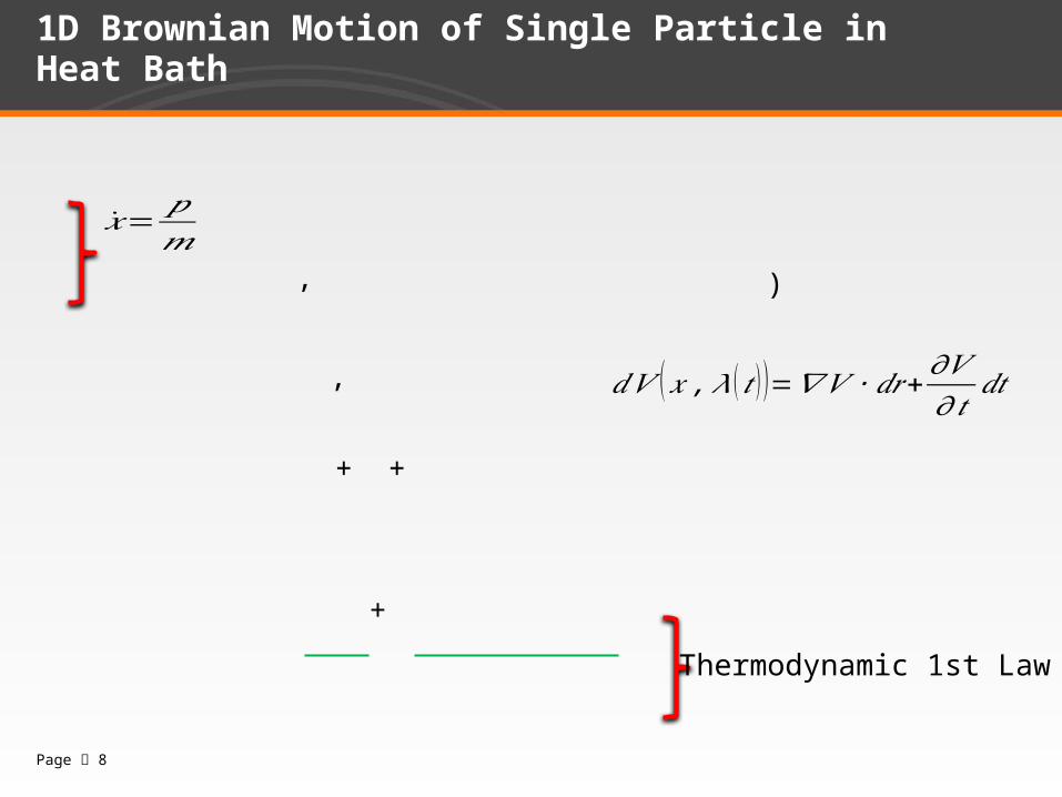
1D Brownian Motion of Single Particle in Heat Bath

�̇�=𝑝𝑚

,

+

)

Thermodynamic 1st Law

,

+ +

𝑑𝑉 (𝑥 ,𝜆 (𝑡 ) )=𝛻𝑉 ∙𝑑𝑟 +𝜕𝑉𝜕𝑡

𝑑𝑡

1D Brownian Motion of Single Particle in Heat Bath

+

Thermodynamic 1st Law

In equilibrium, =0 ,𝑑𝐸𝑑𝑡

=−�̇�

�̇�=𝜕𝑉𝜕𝜆

�̇�= 𝜕𝜕𝑘 ( 1

2𝑘𝑥2) �̇�=1

2𝑥2 �̇� =

In non-equilibrium steady state, 0 Work done by external source converts to heat in the heat bath.

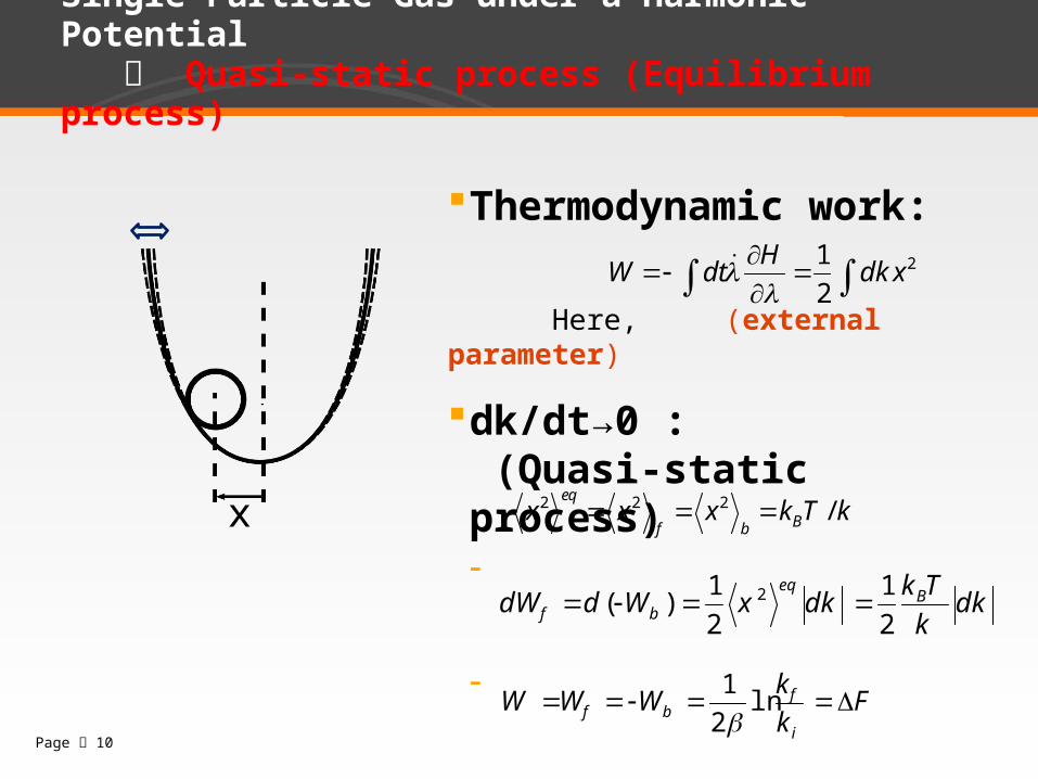
Single Particle Gas under a Harmonic Potential Quasi-static process (Equilibrium process)

Thermodynamic work:

Here, (external parameter)

dk/dt→0 : (Quasi-static process)-

-

-

2

2

1xdk

HdtW

kTkxxx Bbf

eq/222

dkkTk

dkxWddW Beq

bf 21

21

)( 2

Fkk

WWWi

fbf ln

21

x

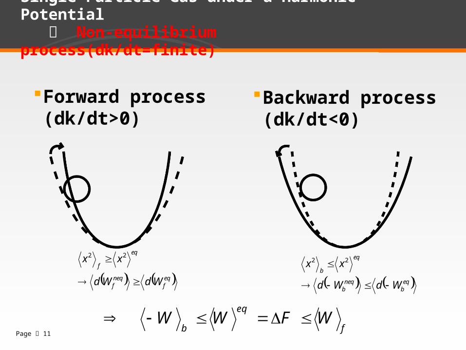
Single Particle Gas under a Harmonic Potential Non-equilibrium process(dk/dt=finite)

Forward process(dk/dt>0)

eqf

neqf

eq

f

WdWd

xx

22

f

eq

bWFWW

Backward process(dk/dt<0)

eqb

neqb

eq

b

WdWd

xx

22

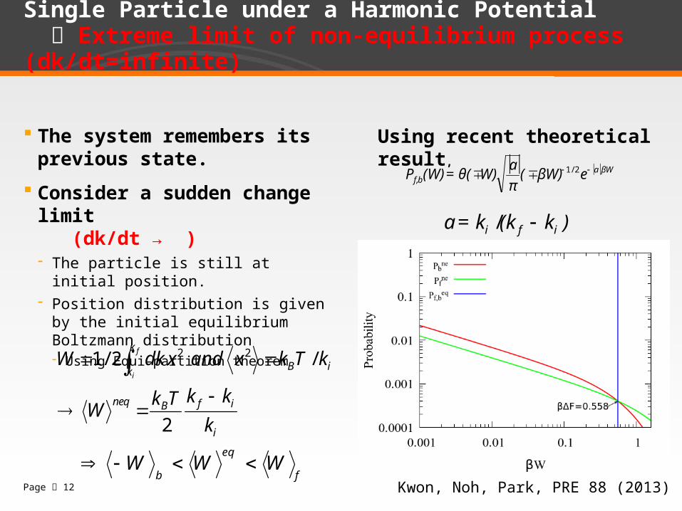
Single Particle under a Harmonic Potential Extreme limit of non-equilibrium process (dk/dt=infinite)

The system remembers its previous state.

Consider a sudden change limit (dk/dt → )- The particle is still at initial position.- Position distribution is given by the initial

equilibrium Boltzmann distribution- Using Equi-partition theorem

i

ifBneq

iB

k

k

k

kkTkW

kTkxandxdkWf

i

2

/2/1 22

f

eq

bWWW

βWabf, eβW)(

π

aW)θ(=(W)P 2/1

)k(kk=a ifi /

Using recent theoretical result,

Kwon, Noh, Park, PRE 88 (2013)

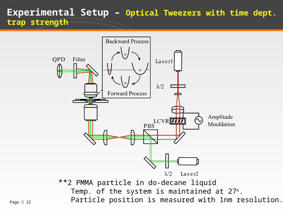
Experimental Setup – Optical Tweezers with time dept. trap strength

**2 PMMA particle in do-decane liquid Temp. of the system is maintained at 27o. Particle position is measured with 1nm resolution.

O

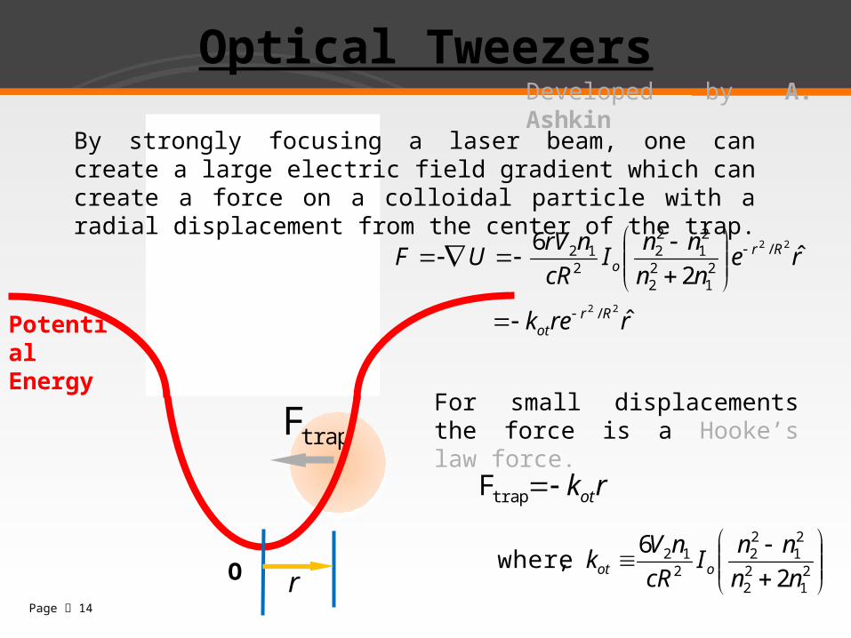
Optical Tweezers

By strongly focusing a laser beam, one can create a large electric field gradient which can create a force on a colloidal particle with a radial displacement from the center of the trap.

For small displacements the force is a Hooke’s law force.

rrek

renn

nnI

cR

nrVUF

Rrot

Rro

ˆ

ˆ2

6

22

22

/

/21

22

21

22

212

rkottrapF

r

trapF

Developed by A. Ashkin

Potential Energy

21

22

21

22

212

2

6,where

nn

nnI

cR

nVk oot

Control of the Trap Strength

The optical trap strength is proportional to the laser power.

Therefore, when the laser power is changed linearly in time, the optical strength should be increased or decreased linearly in time.

The laser power is controlled using LCVR(Liquid Crystal Variable Retarders) which allows manipulation of polarization states by applying an electric field to the liquid crystal.

Laser Power Stability

Since the optical trap strength is proportional to the laser power, it is important to have a stable laser power in time.

A feedback control of the laser power is used to reduce the long time fluctuation of the laser power.

During the experiment, the fluctuation of laser power is less than ±0.5%.

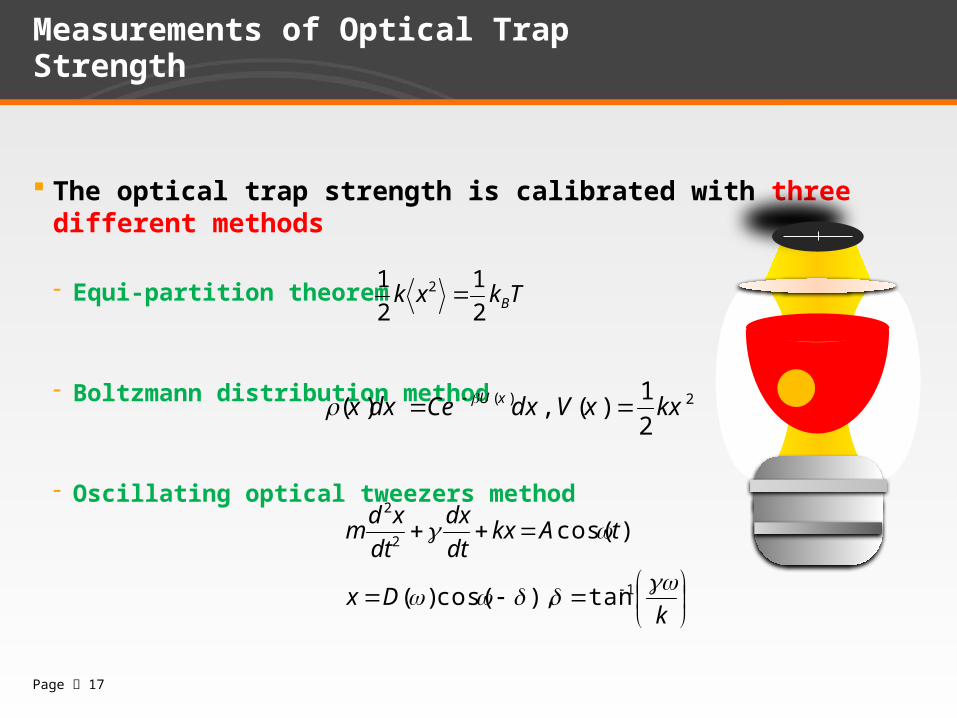
Measurements of Optical Trap Strength

The optical trap strength is calibrated with three different methods

- Equi-partition theorem

- Boltzmann distribution method

- Oscillating optical tweezers method

Tkxk B2

1

2

1 2

2)(

21

)(,)( kxxVdxCedxx xU

kDx

tAkxdt

dx

dt

xdm

1

2

2

tan),cos()(

)cos(

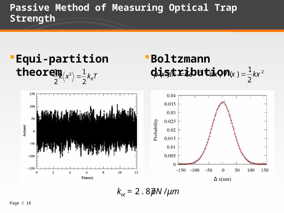
Passive Method of Measuring Optical Trap Strength

Equi-partition theorem Boltzmann distribution2)(

21

)(,)( kxxVdxCedxxp xV Tkxk B2

1

2

1 2

μmpN=kot /2.87

Tracking beam

Boltzmann Statistics

100 XOil

NA 1.35

Objective

Potential Energy

Condenser

QPD

CTkxpTkxV

DimindxCedxxp

BB

TkxV

B

ln)(ln)(

1)()(

2

21

)( xkxV OT

Profile of 1D Harmonic Potential

μmpN=kot /2.87

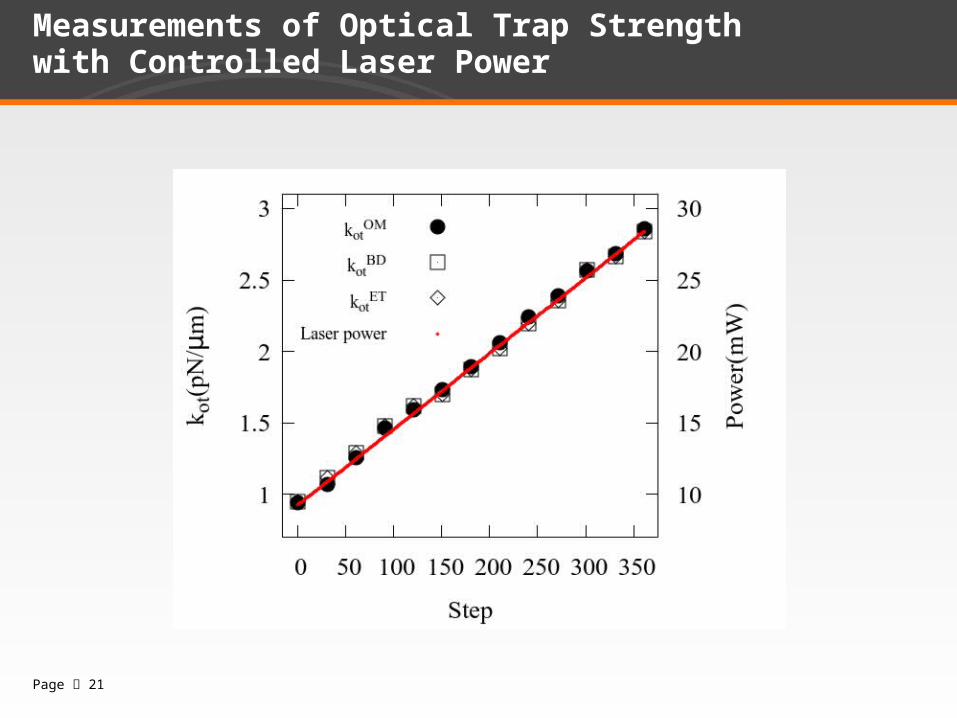
Measurements of Optical Trap Strengthwith Controlled Laser Power

Experimental Setup – Optical Tweezers with time dept. trap strength

**2 PMMA particle in do-decane liquid Temp. of the system is maintained at 27o. Particle position is measured with 1nm resolution.

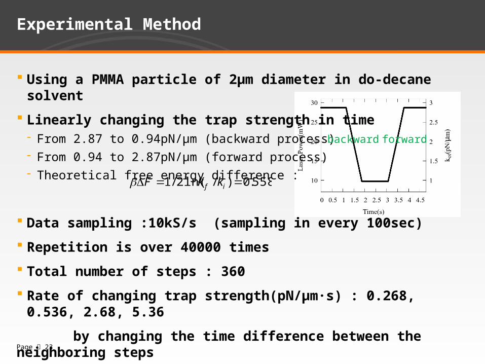
Experimental Method

Using a PMMA particle of 2µm diameter in do-decane solvent

Linearly changing the trap strength in time - From 2.87 to 0.94pN/µm (backward process) - From 0.94 to 2.87pN/µm (forward process)- Theoretical free energy difference :

Data sampling :10kS/s (sampling in every 100sec)

Repetition is over 40000 times

Total number of steps : 360

Rate of changing trap strength(pN/µm·s) : 0.268, 0.536, 2.68, 5.36

by changing the time difference between the neighboring steps

from 1msec to 20msec

558.0)/ln(2/1 if kkF

backward forward

Laser Power and Trap Strength in Time

forwardbackward

EQ EQEQ

sμmpN±=k /0.536

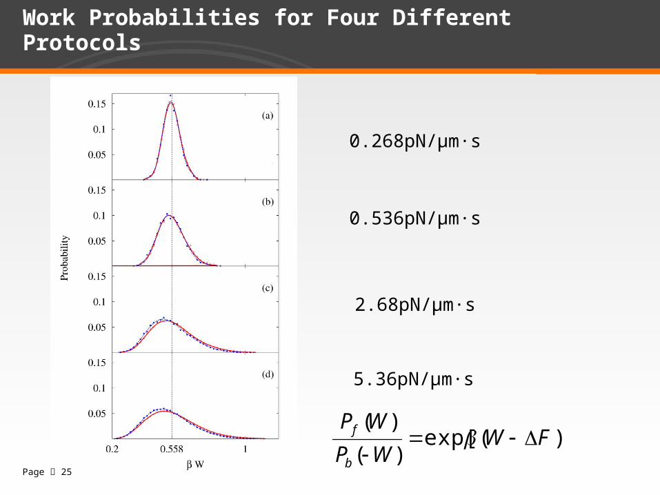
Work Probabilities for Four Different Protocols

5.36pN/µm·s

0.268pN/µm·s

0.536pN/µm·s

2.68pN/µm·s

)](exp[)(

)(FW

WP

WP

b

f

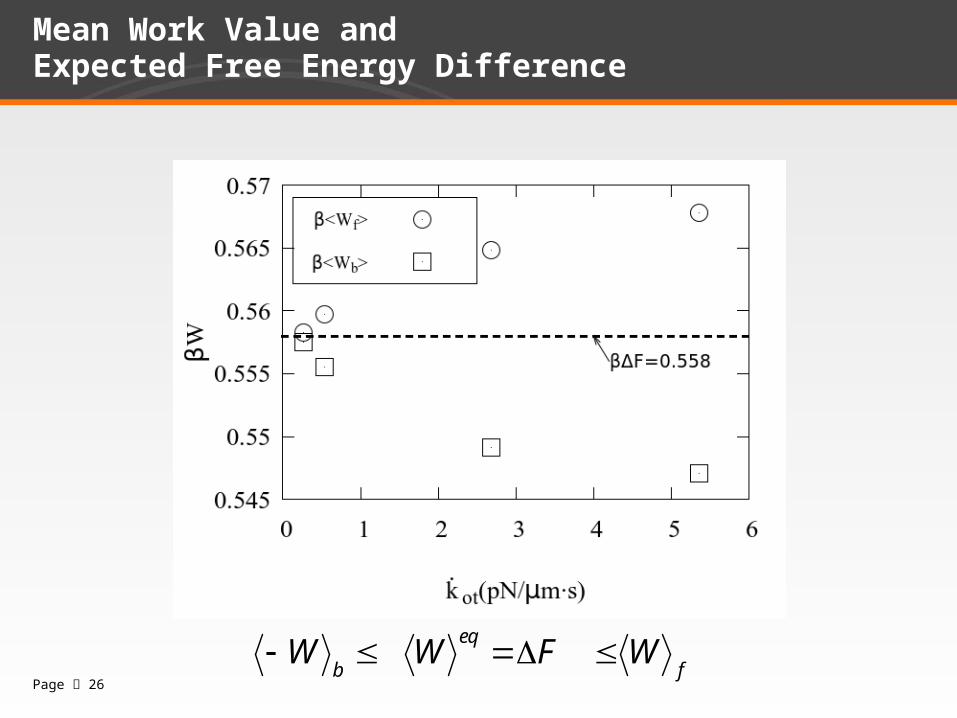
Mean Work Value and Expected Free Energy Difference

f

eq

bWFWW

Verification of Crooks Fluctuation Theorem

Fastest protocol, 5.36pN/µm·s Fast protocol, 2.68pN/µm·s

)](exp[)(

)(FW

WP

WP

b

f

Conclusion

We experimentally demonstrated the CFT in an exactly solvable real system.

We also showed that mean works obey in non-equilibrium processes.

Useful to make a micrometer-sized stochastic heat engine.

f

eq

bWWW

)](exp[)(

)(FW

WP

WP

b

f

Thank you for your attentions.

Supplement

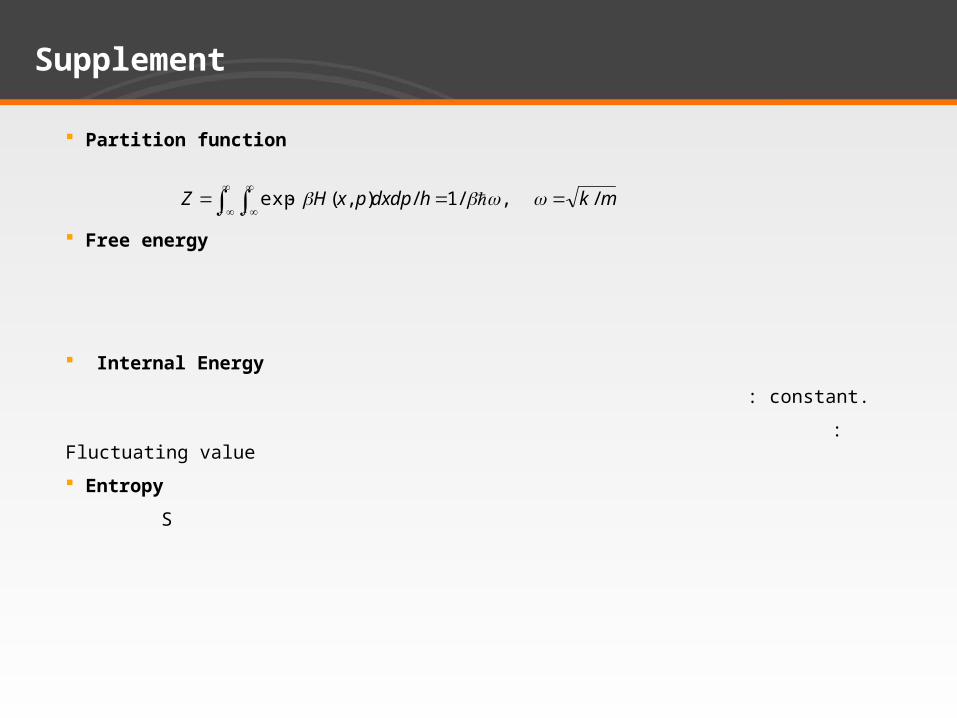
Partition function

Free energy

Internal Energy

: constant. : Fluctuating value Entropy S

mkhdxdppxHZ /,/1/),(exp

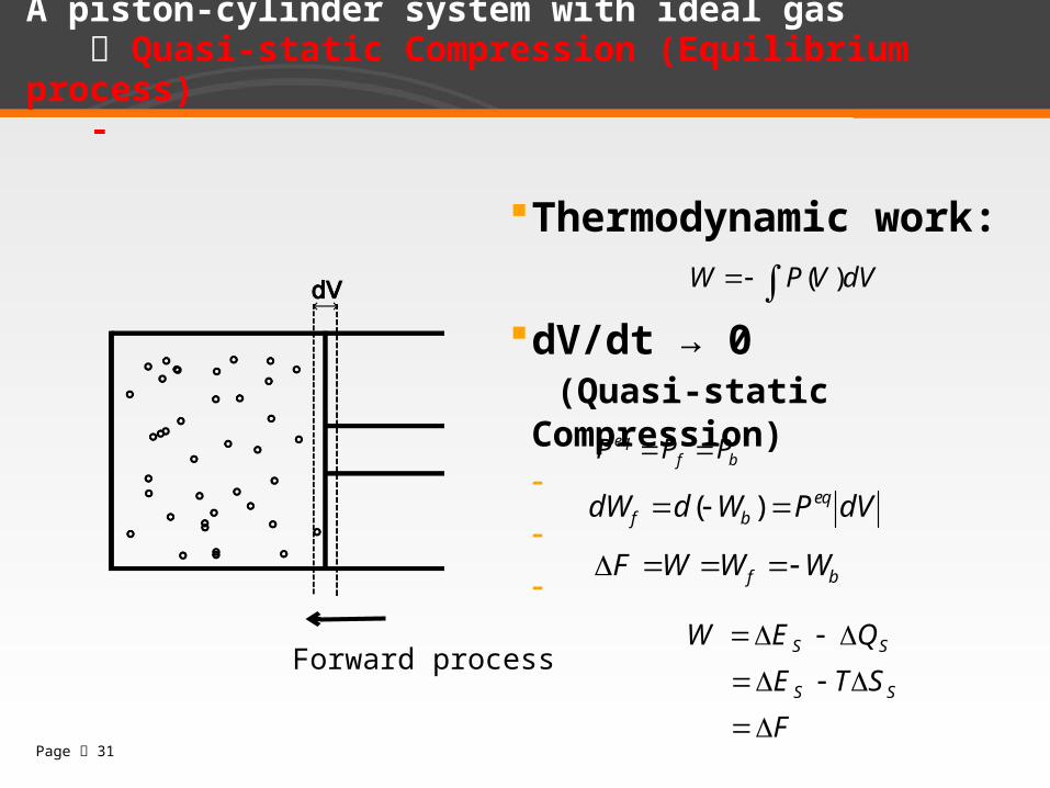
A piston-cylinder system with ideal gas Quasi-static Compression (Equilibrium process) -

Thermodynamic work:

dV/dt → 0 (Quasi-static Compression)- - -

Forward process

dVVPW )(

bfeq PPP

dVPWddW eqbf )(

bf WWWF

F

STE

QEW

SS

SS

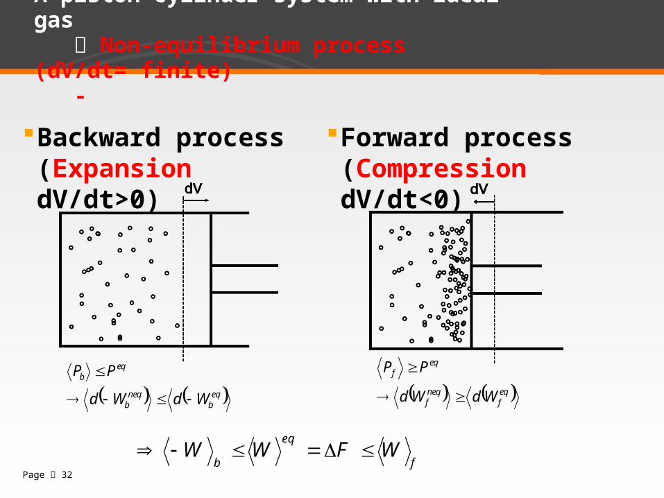
Backward process (Expansion dV/dt>0)

Forward process(Compression dV/dt<0)

eqb

neqb

eqb

WdWd

PP

eqf

neqf

eqf

WdWd

PP

f

eq

bWFWW

A piston-cylinder system with ideal gas Non-equilibrium process (dV/dt= finite) -

O O’

t

tx

d

),(dFdrag

),(cosFtrap txtAkot

),( tx

tA cosReference

position

a

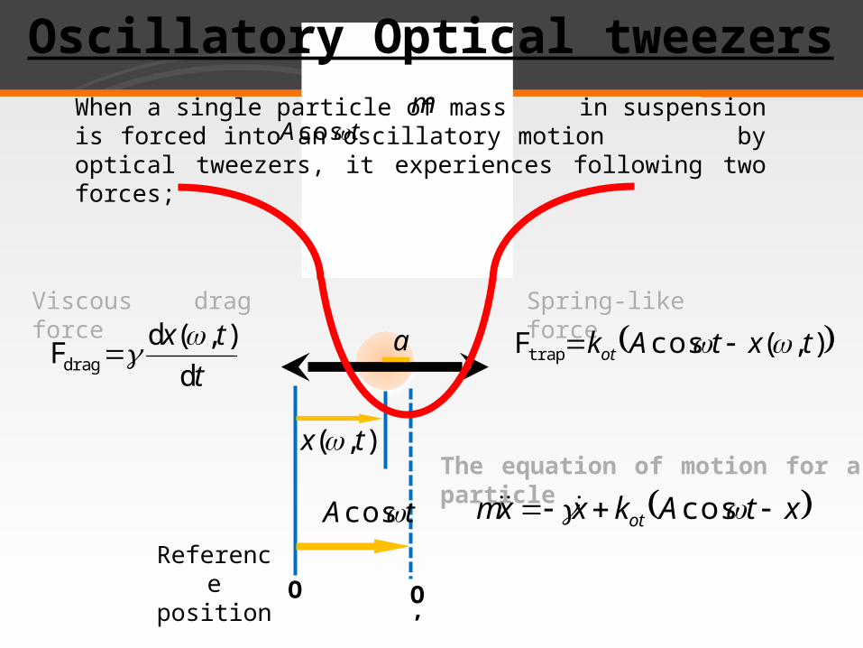
When a single particle of mass in suspension is forced into an oscillatory motion by optical tweezers, it experiences following two forces;

tA cos

Viscous drag force Spring-like force

The equation of motion for a particle

xtAkxxm ot cos

m

Oscillatory Optical tweezers

Oscillatory Optical tweezers

2

2cosOT OT

d x dxm k x k A tdt dt

( , ) ( ) cos ( )x t D t

2 2

( ) OT

OT

kD

A k

1( ) tan

OTk

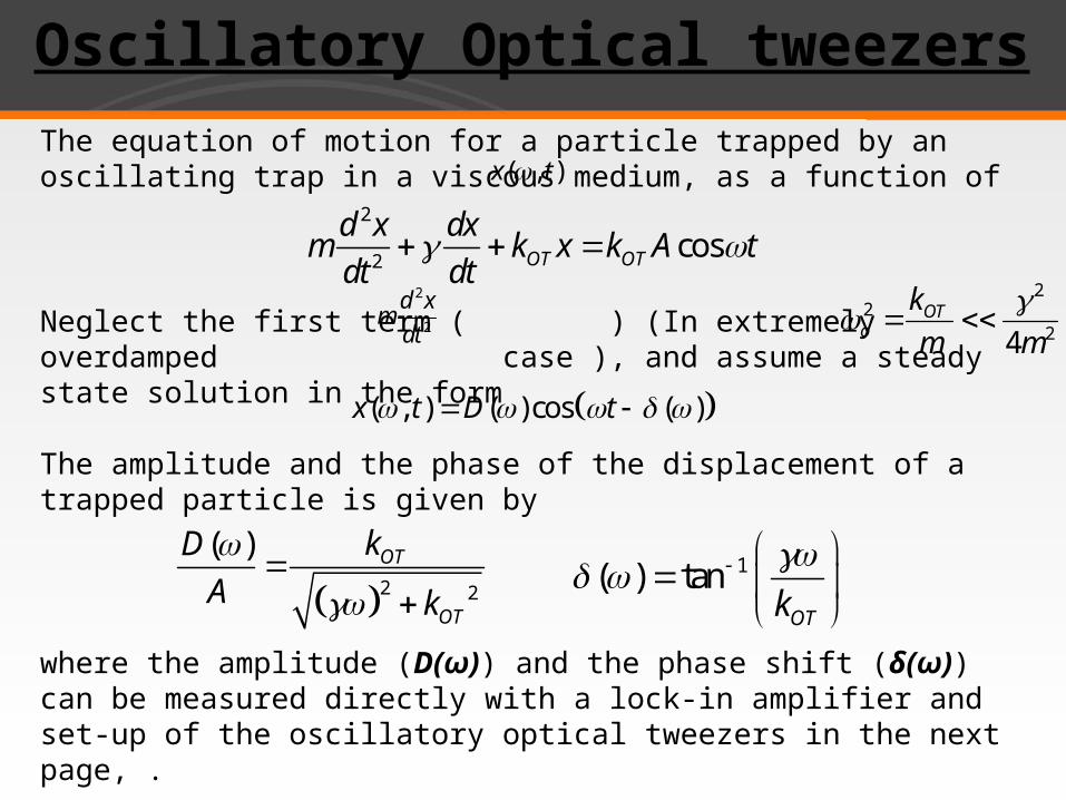
The equation of motion for a particle trapped by an oscillating trap in a viscous medium, as a function of

Neglect the first term ( ) (In extremely overdamped case ), and assume a steady state solution in the form

2

2

d xmdt

The amplitude and the phase of the displacement of a trapped particle is given by

where the amplitude (D(ω)) and the phase shift (δ(ω)) can be measured directly with a lock-in amplifier and set-up of the oscillatory optical tweezers in the next page, .

( , )x t

2

22

4mm

kOTo

Active Method of Measuring Optical Trap Strength

Equation of motion

Phase delay

k

1tan

Fixed potential well Horizontally oscillating potential well

)(cos ωtA=x(t)k+(t)xγ+(t)xm ot

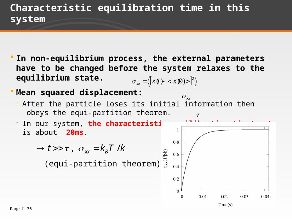
Characteristic equilibration time in this system

In non-equilibrium process, the external parameters have to be changed before the system relaxes to the equilibrium state.

Mean squared displacement: - After the particle loses its initial information then obeys the equi-partition

theorem.- In our system, the characteristic equilibration time( ) is about 20ms.

2)0()( xtxxx

kTkt Bxx /,

xx

(equi-partition theorem)

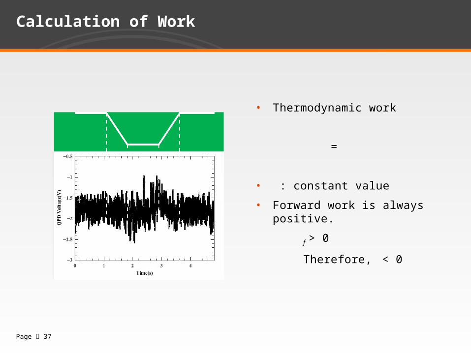
Calculation of Work

• Thermodynamic work

=

• : constant value

• Forward work is always posi-tive.

f > 0

Therefore, < 0

Work Probability : Slowest protocol, 0.268pN/µm·s

Work Probability : Slow protocol, 0.536pN/µm·s

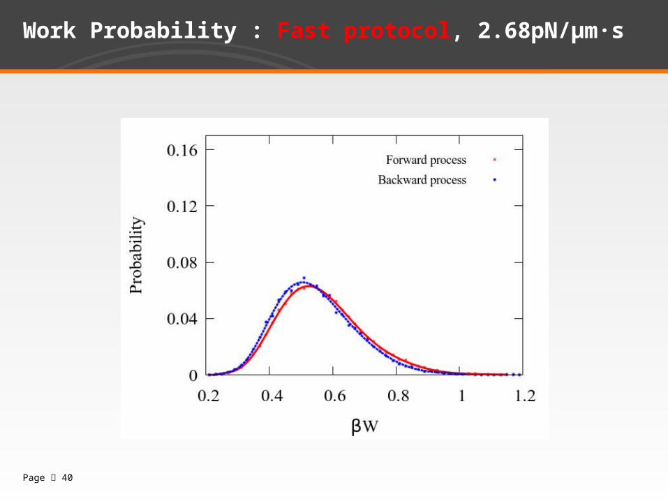
Work Probability : Fast protocol, 2.68pN/µm·s

Work Probability : Fastest protocol, 5.36pN/µm·s

Lee Dong-yun¹, Chulan Kwon², Hyuk Kyu Pak¹ Department of physics, Pusan National University,...

Documents

Transcript of Lee Dong-yun¹, Chulan Kwon², Hyuk Kyu Pak¹ Department of physics, Pusan National University,...