Lectures on

Topics in Algebraic Number Theory

Sudhir R. GhorpadeIndian Institute of Technology Bombay

Mathematisches Seminar, Bereich IIChristian-Albrechts-Universitat zu Kiel

Kiel, GermanyDecember 2000

© Sudhir R. GhorpadeDepartment of MathematicsIndian Institute of Technology BombayPowai, Mumbai 400 076, India

E-Mail: srg@math.iitb.ac.in

URL: http://www.math.iitb.ac.in/∼srg/

Version 1.2, May 3, 2008[Original Version (1.0): January 7, 2002]

2

Preface

During December 2000, I gave a course of ten lectures on Algebraic Number Theory at the Universityof Kiel in Germany. These lectures were aimed at giving a rapid introduction to some basic aspects ofAlgebraic Number Theory with as few prerequisites as possible. I had also hoped to cover some parts ofAlgebraic Geometry based on the idea, which goes back to Dedekind, that algebraic number fields andalgebraic curves are analogous objects. But in the end, I had no time to discuss any Algebraic Geometry.However, I tried to be thorough in regard to the material discussed and most of the proofs were eitherexplained fully or at least sketched during the lectures. These lecture notes are a belated fulfillment ofthe promise made to the participants of my course and the Kieler Graduiertenkolleg. I hope that theywill still be of some use to the participants of my course and other students alike.

The first chapter is a brisk review of a number of basic notions and results which are usuallycovered in the courses on Field Theory or Galois Theory. A somewhat detailed discussion of the notionof norm, trace and discriminant is included here. The second chapter begins with a discussion ofbasic constructions concerning rings, and goes on to discuss rudiments of noetherian rings and integralextensions. Although both these chapters seem to belong to Algebra, they are mostly written with aview towards Number Theory. Chapters 3 and 4 discuss topics such as Dedekind domains, ramificationof primes, class group and class number, which belong more properly to Algebraic Number Theory.Some motivation and historical remarks can be found at the beginning of Chapter 3. Several exercisesare scattered throughout these notes. However, I have tried to avoid the temptation of relegating asexercises some messy steps in the proofs of the main theorems. A more extensive collection of exercisesis available in the books cited in the bibliography, especially [4] and [13].

In preparing these notes, I have borrowed heavily from my notes on Field Theory and RamificationTheory for the Instructional School on Algebraic Number Theory (ISANT) held at Bombay Universityin December 1994 and to a lesser extent, from my notes on Commutative Algebra for the InstructionalConference on Combinatorial Topology and Algebra (ICCTA) held at IIT Bombay in December 1993.Nevertheless, these notes are neither a subset nor a superset of the ISANT Notes or the ICCTA notes. Inorder to make these notes self-contained, I have inserted two appendices in the end. The first appendixcontains my Notes on Galois Theory, which have been in private circulation at least since October 1994.The second appendix reproduces my recent article in Bona Mathematica which gives a leisurely accountof discriminants. There is a slight repetition of some of the material in earlier chapters but this articlemay be useful for a student who might like to see some connection between the discriminant in thecontext of field extensions and the classical discriminant such as that of a quadratic.

It is a pleasure to record my gratitude to the participants of my course, especially, Andreas Baltz,Hauke Klein and Prof. Maxim Skriganov for their interest, and to the Kiel graduate school “EfficientAlgorithms and Multiscale Methods” of the German Research Foundation (“Deutsche Forschungsge-meinschaft”) for its support. I am particularly grateful to Prof. Dr. Anand Srivastav for his keeninterest and encouragement. Comments or suggestions concerning these notes are most welcome andmay be communicated to me by e-mail. Corrections or future revisions to these notes will be posted onmy web page at http://www.math.iitb.ac.in/∼srg/Lecnotes.html and the other notes mentionedin the above paragraph will also be available here.

Mumbai, January 7, 2002 Sudhir Ghorpade

3

Contents

1 Field Extensions 6

1.1 Basic Facts . . . . . . . . . . . . . . . . . . . . . . . . . . . . . . . . . . . . . . . 6

1.2 Basic Examples . . . . . . . . . . . . . . . . . . . . . . . . . . . . . . . . . . . . . 9

1.3 Norm, Trace and Discriminant . . . . . . . . . . . . . . . . . . . . . . . . . . . . 12

2 Ring Extensions 15

2.1 Basic Processes in Ring Theory . . . . . . . . . . . . . . . . . . . . . . . . . . . . 15

2.2 Noetherian Rings and Modules . . . . . . . . . . . . . . . . . . . . . . . . . . . . 17

2.3 Integral Extensions . . . . . . . . . . . . . . . . . . . . . . . . . . . . . . . . . . . 19

2.4 Discriminant of a Number Field . . . . . . . . . . . . . . . . . . . . . . . . . . . . 21

3 Dedekind Domains and Ramification Theory 26

3.1 Dedekind Domains . . . . . . . . . . . . . . . . . . . . . . . . . . . . . . . . . . . 27

3.2 Extensions of Primes . . . . . . . . . . . . . . . . . . . . . . . . . . . . . . . . . . 32

3.3 Kummer’s Theorem . . . . . . . . . . . . . . . . . . . . . . . . . . . . . . . . . . 35

3.4 Dedekind’s Discriminant Theorem . . . . . . . . . . . . . . . . . . . . . . . . . . 37

3.5 Ramification in Galois Extensions . . . . . . . . . . . . . . . . . . . . . . . . . . . 38

3.6 Decomposition and Inertia Groups . . . . . . . . . . . . . . . . . . . . . . . . . . 40

3.7 Quadratic and Cyclotomic Extensions . . . . . . . . . . . . . . . . . . . . . . . . 42

4 Class Number and Lattices 46

4.1 Norm of an ideal . . . . . . . . . . . . . . . . . . . . . . . . . . . . . . . . . . . . 46

4.2 Embeddings and Lattices . . . . . . . . . . . . . . . . . . . . . . . . . . . . . . . 48

4.3 Minkowski’s Theorem . . . . . . . . . . . . . . . . . . . . . . . . . . . . . . . . . 52

4.4 Finiteness of Class Number and Ramification . . . . . . . . . . . . . . . . . . . . 53

Bibliography 56

A Appendix: Notes on Galois Theory 57

A.1 Preamble . . . . . . . . . . . . . . . . . . . . . . . . . . . . . . . . . . . . . . . . 57

A.2 Field Extensions . . . . . . . . . . . . . . . . . . . . . . . . . . . . . . . . . . . . 58

A.3 Splitting Fields and Normal Extensions . . . . . . . . . . . . . . . . . . . . . . . 60

A.4 Separable Extensions . . . . . . . . . . . . . . . . . . . . . . . . . . . . . . . . . . 62

A.5 Galois Theory . . . . . . . . . . . . . . . . . . . . . . . . . . . . . . . . . . . . . . 63

A.6 Norms and Traces . . . . . . . . . . . . . . . . . . . . . . . . . . . . . . . . . . . 67

4

B Appendix: Discriminants in Algebra and Arithmetic 70B.1 Discriminant in High School Algebra . . . . . . . . . . . . . . . . . . . . . . . . . 70B.2 Discriminant in College Algebra . . . . . . . . . . . . . . . . . . . . . . . . . . . . 74B.3 Discriminant in Arithmetic . . . . . . . . . . . . . . . . . . . . . . . . . . . . . . 77

References . . . . . . . . . . . . . . . . . . . . . . . . . . . . . . . . . . . . . . . . 82

5

Chapter 1

Field Extensions

We begin with a quick review of the basic facts regarding field extensions. For more details,consult Appendix A or any of the standard texts such as Lang [11] or Jacobson [9].

1.1 Basic Facts

Suppose L/K is a field extension (which means that L is a field and K is a subfield of L). We callL/K to be finite if as a vector space over K, L is of finite dimension; the degree of L/K, denotedby [L : K], is defined to be the vector space dimension of L over K. Given α1, . . . , αn ∈ L,we denote by K(α1, . . . , αn) (resp: K[α1, . . . , αn]) the smallest subfield (resp: subring) of Lcontaining K and the elements α1, . . . , αn. If there exist finitely many elements α1, . . . , αn ∈ Lsuch that L = K(α1, . . . , αn), then L/K is said to be finitely generated. An element α ∈ L suchthat L = K(α) is called a primitive element, and if such an element exists, then L/K is said tobe a simple extension. If L′/K is another extension, then a homomorphism σ : L→ L′ such thatσ(c) = c for all c ∈ K is called a K–homomorphism of L→ L′. Note that a K–homomorphismis always injective and if [L : K] = [L′ : K], then it is surjective. Thus if L = L′, then such mapsare called K–automorphisms of L. The set of all K–automorphisms of L is clearly a group wherethe group operation defined by composition of maps. This is called the Galois group of L/K andis denoted by Gal(L/K) or G(L/K). Given any subgroup H of the group of automorphisms ofL, we can associate a subfield LH of L defined by LH = α ∈ L : σ(α) = α for all σ ∈ H; thisis called the fixed field of H.

An element α ∈ L is said to be algebraic over K if it satisfies a nonzero polynomial withcoefficients in K. Suppose α ∈ L is algebraic over K. Then a nonzero polynomial of leastpossible degree satisfied by α is clearly irreducible and, moreover, it is unique if we require itto be monic; this monic irreducible polynomial will be denoted by Irr(α,K), and called theminimal polynomial of α over K. The extension L/K is said to be algebraic if every α ∈ L isalgebraic over K. If L/K is algebraic, then we call it separable if Irr(α,K) has distinct roots(in some extension of K) for every α ∈ L, and we call it normal if Irr(α,K) has all its roots inL for every α ∈ L. It may be noted that if L/K is algebraic, then it is normal if and only ifany K–homomorphism of L into some extension L′ of L maps L onto itself. We call L/K tobe a Galois extension if it is finite, separable and normal.

To check separability, one generally uses the fact that an irreducible polynomial in K[X] has

6

distinct roots iff (= if and only if) its derivative is a nonzero polynomial. This fact follows, inturn, from the elementary observation that a root α of a polynomial f(X) ∈ K[X] is a multipleroot iff f ′(α) = 0. The above fact can be used to show that K is perfect (which means eitherthe characteristic of K is 0 or the characteristic of K is p 6= 0 and K = Kp, i.e., for any x ∈ K,there exists y ∈ K such that x = yp) iff every algebraic extension of K is separable. On theother hand, normality can be checked using the fact a finite extension of K is normal iff it isthe “splitting field” of some polynomial in K[X]. Recall that given a nonconstant polynomialf(X) ∈ K[X], we can find an extension E of K such that f(X) splits into linear factors inE[X], and E is generated over K by the roots of f(X) in E. Such an extension is unique upto a K–isomorphism, and is called the splitting field of f(X) over K. If deg f(X) = n, thenthe degree of the splitting field of f(X) over K is at most n!. Thus if f(X) is a nonconstantpolynomial in K[X] having distinct roots, and L is its splitting field over K, then L/K is anexample of a Galois extension. A K–automorphism of L permutes the roots of f(X), and thispermutation uniquely determines the automorphism. Thus Gal(L/K) may be thought of asa finite group of permutations. In this case, Gal(L/K) is also called the Galois group of thepolynomial f(X) or of the equation f(X) = 0.

Some basic results regarding field extensions are the following.

(i) L/K is finite ⇐⇒ L/K is algebraic and finitely generated.

(ii) Given any α ∈ L, we have:

α is algebraic over K ⇔ K(α)/K is finite ⇔ K(α) = K[α].

Moreover, if α is algebraic over K and deg Irr(α,K) = n, then 1, α, α2, . . . , αn−1 formsa K–basis of K(α).

(iii) If α1, . . . , αn ∈ L are algebraic, then K(α1, . . . , αn) is an algebraic extension of K. Fur-ther, if α1, . . . , αn are separable over K, then it is also a separable extension. In particular,the elements of L which are algebraic over K form a subfield of L and among these, thosewhich are separable form a smaller subfield.

(iv) Finiteness, algebraicity and separability are “transitive” properties. That is, if E is asubfield of L containing K, then L/K is finite (resp: algebraic, separable) iff both L/Eand E/K are finite (resp: algebraic, separable). Moreover, if L/K is finite, then [L :K] = [L : E][E : K]. In case of normality, all we can say in general is that L/K is normalimplies that L/E is normal1. Thus, a fortiori, the same thing holds for Galois extensions.

(v) (Primitive Element Theorem). If L/K is finite and separable, then it is simple, i.e., thereexists α ∈ L such that L = K(α).

In Number Theory, one has to usually deal with algebraic extensions of Q, the field ofrationals, or of Fp = Z/pZ, the finite field with p elements. Since Q and Fp are clearly perfectfields, every such extension is separable and thus saying that it is Galois amounts to sayingthat it is finite and normal.

1Find examples to show that the other two possible implications are not true.

7

Now we come to the central result in Galois Theory. Suppose L/K is a Galois extension.Then Gal(L/K) is a finite group of order [L : K] and its fixed field is K. In fact, we have aninclusion–reversing one–to–one correspondence between the subgroups of the Galois group ofL/K and the intermediate fields between K and L. This correspondence is given as follows.Given an intermediate field E (i.e., a subfield of L containing K), the corresponding subgroup ofGal(L/K) is Gal(L/E). And given a subgroup H of Gal(L/K), the corresponding intermediatefield is the fixed field LH of H. Moreover, given a subfield E of L containing K, the “bottompart” E/K is Galois iff Gal(L/E) is a normal subgroup of Gal(L/K), and if this is the case,then Gal(E/K) is isomorphic to the factor group Gal(L/K)/Gal(L/E). The above result isusually called the Fundamental Theorem of Galois Theory.

Adjectives applicable to a group are generally inherited by a Galois extension. Thus a Galoisextension is said to be abelian if its Galois group is abelian, and it is said to be cyclic if itsGalois group is cyclic.

Before ending this section, we make some remarks about the important notion of composi-tum (or composite) of fields, which is very useful in Algebraic Number Theory. Let E and Fbe subfields of the field L. The compositum (or the composite) of E and F (in L), denoted byEF , is defined to be the smallest subfield of L containing both E and F . The compositum ofan arbitrary family of subfields of L is defined in a similar fashion; we use an obvious analogueof the above notation in case of a finite family of subfields. Now suppose K is a subfield of bothE and F , i.e., a subfield of the field E ∩ F . We list below some elementary facts concerningcompositum of fields, which the reader may prove as exercises.

(i) If E/K is finitely generated (resp: finite, algebraic, separable, normal, Galois, abelian),then so is EF/F .

(ii) If both E/K and F/K are finitely generated (resp: finite, algebraic, separable, normal,Galois, abelian), then so is EF/K.

(iii) If E/K is Galois, then the map σ → σ|E defines an isomorphism of Gal(EF/F ) with thesubgroup Gal(E/E ∩ F ) of Gal(E/K). If both E/K and F/K are Galois, then the mapσ → (σ|E , σ|F ) defines an isomorphism of Gal(EF/K) with the subgroup Gal(E/E∩F )×Gal(F/E∩F ) of Gal(E/K)×Gal(F/K). In particular, if E∩F = K, then we have naturalisomorphisms Gal(EF/F ) ≃ Gal(E/K) and Gal(EF/K) ≃ Gal(E/K) ×Gal(F/K).

Observe that in view of the above properties, we can define the maximal abelian extensionof K in L (as the compositum of all abelian extensions of K contained in L).

Exercise 1.1. Suppose L/K is a Galois extension. Let H1 and H2 be subgroups of Gal(L/K),and E1 and E2 be their fixed fields respectively. Show that the fixed field of H1 ∩ H2 is thecompositum E1E2 whereas the fixed field of the smallest subgroup H of Gal(L/K) containingH1 and H2 (note that if either H1 or H2 is normal, then H = H1H2) is E1 ∩ E2.

Exercise 1.2. Let L1, . . . , Lr be Galois extensions of K with Galois groups G1, . . . , Gr respec-tively. Suppose for 1 ≤ i < r we have Li+1 ∩ (L1L2 . . . Li) = K. Then show that the Galoisgroup of L1L2 . . . Lr is isomorphic to G1 ×G2 × · · · ×Gr.

Exercise 1.3. Suppose L/K is Galois and Gal(L/K) can be written as a direct product G1 ×· · · × Gr. Let Li be the fixed field of the subgroup G1 × . . . Gi−1 × 1 × Gi+1 × · · · × Gr

8

of G. Show that Li/K is Galois with Gal(Li/K) ≃ Gi, and Li+1 ∩ (L1L2 . . . Li) = K, andL1L2 . . . Lr = L.

1.2 Basic Examples

In this section, we will discuss some examples of Galois extensions, which are quite importantin Number Theory and Algebra.

Example 1: Quadratic Extensions.

An extension of degree 2 is called a quadratic extension. Let L/K be a quadratic extension.Suppose α ∈ L is any element such that α /∈ K. Then [K(α) : K] must be > 1 and itmust divide [L : K] = 2. Therefore L = K(α) and α satisfies an irreducible quadratic, sayX2 + bX + c, with coefficients in K. The other root, say β, of this quadratic must satisfyα + β = −b, and hence it is also in L. So L/K is normal. Also if char K 6= 2, then clearlyβ 6= α and so L/K is separable as well. Thus a quadratic extension is always a Galois extensionexcept possibly in characteristic two. Now assume that char K 6= 2. Then Gal(L/K) is a groupof order 2, and the nonidentity element in it is the automorphism of L which maps α to β.Using the (Shreedharacharya’s) formula for roots of quadratic polynomial, we can replace αby√

a so that L = K(√

a), where a is some element of K and√

a denotes an element of Lwhose square is a. With this, we can write L = r + s

√a : r, s ∈ K and Gal(L/K) = id, σ,

where id denotes the identity automorphism of L and σ is the K–automorphism defined byσ(r + s

√a) = r − s

√a.

If K = Q and L is a subfield of C such that [L : Q] = 2, then it is called a quadratic field.In general, a subfield of C which is of finite degree over Q is known as an algebraic number fieldor simply, a number field. In view of the above discussion, we easily see that if L is a quadraticfield, then there exists a unique squarefree integer m, with m 6= 0, 1, such that L = Q(

√m). We

say that L is a real quadratic field or imaginary quadratic field according as m > 0 or m < 0.

Exercise 1.4. Suppose L/K is a biquadratic extension, i.e., L = K(α, β) where α, β are elementsof L which are not in K but whose squares are distinct elements of K. Assume that char K 6= 2.Show that L/K is a Galois extension and compute its Galois group.

Example 2: Cyclotomic Extensions.

Let k be a field and n be a positive integer. An element ω ∈ k such that ωn = 1 is calledan nth root of unity (in k). Let µn = µn(k) denote the set of all nth roots of unity in k. Thenµn is a finite subgroup of the multiplicative group k∗ of nonzero elements of k, and thereforeit is cyclic. Any generator of µn is called a primitive nth root of unity in k. For example,if k = C, then ζ = ζn = e2πi/n is a primitive nth root of unity, and µn(C) consists of then elements 1, ζ, ζ2, . . . , ζn−1; among these the elements ζj where (j, n) = 1, are precisely theprimitive nth roots of unity (verify!). The subfield Q(ζ) of C generated by ζ over Q is calledthe nth cyclotomic field, and the extension Q(ζ)/Q is called a cyclotomic extension. Since thepolynomial Xn − 1 splits into distinct linear factors in Q(ζ)[X] as

Xn − 1 =

n−1∏

i=0

(X − ζi)

9

we see that Q(ζ)/Q is a Galois extension whose degree is at most n. Suppose G = Gal(Q(ζ)/Q)and σ ∈ G. Then σ(ζ) must also be a root of Xn − 1, and therefore σ(ζ) = ζj for some integerj = j(σ). It is clear that σ uniquely determines j(σ) modulo n. Hence the map σ → j(σ) isinjective. Moreover, if σ, τ ∈ G, then we have j(στ) = j(σ)j(τ)(mod n). Since G is a group,we see that j(σ)(mod n) is a unit in Z/nZ, and σ → j(σ) defines an injective homomorphismof G into (Z/nZ)×, the multiplicative group of units2 in Z/nZ. It follows that G is abelian andits order is at most ϕ(n), where ϕ is the Euler totient function defined by

ϕ(n) = the number of positive integers ≤ n and relatively prime to n.

We will now show that the order of G, i.e., [Q(ζ) : Q], is exactly equal to ϕ(n), which will implythat the Galois group of Q(ζ)/Q is naturally isomorphic to (Z/nZ)×. For this, we need thefollowing elementary fact which will be proved later in Section 2.4.

FACT: If a monic polynomial with integer coefficients factors as f(X)g(X), where f(X) andg(X) are monic polynomials with rational coefficients, then the coefficients of f(X) and g(X)must be integers.

To prove the earlier assertion, let Φn(X) denote the minimal polynomial of ζ = ζn over Q.Then it must divide Xn − 1 in Q[X]. Hence by the FACT above, Φn(X) must have integercoefficients and Xn − 1 = Φn(X)g(X), for some monic polynomial g(X) ∈ Z[X]. Now let p bea prime number which doesn’t divide n and α be a root of Φn(X). We claim that αp must alsobe a root of Φn(X). To prove the claim, assume the contrary. Then αp is a root of g(X) andhence α is a root of g(Xp). Thus g(Xp) = Φn(X)h(X) for some h(X) ∈ Z[X] (using the FACTonce again!). Now reduce (mod p), i.e., consider the polynomials g(X), h(X), etc obtained byreducing the coefficients of g(X), h(X), etc., (mod p). Then (by Fermat’s little theorem!), wefind that (g(X))p = g(Xp) = Φn(X)h(X). This implies that g(X) and Φn(X) have a commonroot, and therefore the polynomial Xn − 1 in Z/pZ[X] has a multiple root. But the latter isimpossible since the derivative of Xn − 1 is nXn−1, which has zero as its only root since n isnot divisible by p. This proves our claim, and, as a consequence, it follows that ζj is a root ofΦn(X) for all integers j such that (j, n) = 1. Hence we find that |G| = [Q(ζ) : Q] = deg Φn(X)is ≥ ϕ(n). This together with the previous argument proves the equality. We also find that

Irr(ζ, Q) = Φn(X) =∏

0≤j≤n−1

(j,n)=1

(X − ζj).

The above polynomial is called the nth cyclotomic polynomial. As noted above, it has integercoefficients and its degree is ϕ(n). Collating the terms suitably in the product representationof Xn − 1, we readily see that

Xn − 1 =∏

d|nΦd(X)

2The structure of this group is well–known from Elementary Number Theory. To begin with, if n = pe11 . . . p

egg

is the factorization of n as a product of powers of distinct primes, then by Chinese Remainder Theorem [see, forexample. Prop. 2.3 in the next chapter], we have (Z/nZ)× ≃ (Z/pe1

1 Z)× × · · · × (Z/pegg Z)×. If p is a prime and

e a positive integer, then (Z/peZ)× is cyclic if p is odd or p = 2 and e ≤ 2. If e > 2, then (Z/2eZ)× is the directproduct of Z/2Z and Z/2e−2Z. In particular, (Z/nZ)× is cyclic, i.e., primitive roots (mod n) exist iff n = 2, 4, pe

or 2pe where p is an odd prime. See, for example, [2] or [8] for details.

10

and so, in particular n =∑

d|n ϕ(d). The above formula, in fact, gives an efficient way tocompute Φn(X) in a recursive manner.

Let m and n be relatively prime positive integers. We know from Elementary NumberTheory, that ϕ is a multiplicative function, and thus ϕ(mn) = ϕ(m)ϕ(n). This implies that[Q(ζmn) : Q] = [Q(ζm) : Q][Q(ζn) : Q]. Moreover, we clearly have that ζm

mn is a primitive nth

root of unity, ζnmn is a primitive mth root of unity, and ζmζn is a primitive mnth root of unity.

Therefore Q(ζmn) must equal the compositum Q(ζm)Q(ζn). This together with the previousequality shows that Q(ζm) ∩Q(ζn) = Q.

Exercise 1.5. If p is a prime number, then show that

Φp(X) =Xp − 1

X − 1= Xp−1 + Xp−2 + · · ·+ X + 1

and for any e ≥ 1, Φpe(X) = Φp(Xpe−1

). Use this and the Eisenstein Criterion for Φpe(X + 1)to show directly that Φpe(X) is irreducible in Q[X].

Exercise 1.6. [This exercise assumes some familiarity with Elementary Number Theory.3] Letp be an odd prime, and ζ be a primitive pth root of unity. Consider the Gauss sum g =∑p−1

t=1

(tp

)

ζt. Show that g2 = (−1)(p−1)/2p. Deduce that the quadratic extension Q(√

p) is

contained in pth or (2p)th cyclotomic extension. Conclude that any quadratic extension iscontained in some cyclotomic extension.

Example 3: Finite fields

Let F be a finite field. Its characteristic must be a prime number, say p. Thus we mayassume that it contains Fp = Z/pZ as a subfield. The extension F/Fp has to be finite and if itsdegree is m, then, evidently, F contains precisely q = pm elements. Now since F ∗ = F \ 0is a group of order q − 1, each of the q elements of F satisfies the polynomial Xq −X. ThusF is a splitting field of Xq − X over Fp. It follows that for any prime power q, there is, upto isomorphism, a unique field of order q. Explicitly, it is the splitting field of Xq − X overZ/pZ. For this reason, one uses the notation Fq or GF (q) to denote a field of order q. Nowsuppose L is a finite extension of F of degree n. Then L is a finite field and |L| = qn. Also, Lis a splitting field over Fp (and hence over F ) of the polynomial Xqn − X which has distinctroots (since its derivative is −1, which is never zero). It follows that L/F is a Galois extension.The map σ : L → L defined by σ(α) = αq is an F–automorphism of L (Verify!). Its powersid, σ, σ2, . . . , σn−1 are distinct because otherwise σi = id for some i with 0 < i < n and thusevery x ∈ L satisfies xqi

= x, which is a contradiction since |L| = qn > qi. Moreover, σn = id.Since Gal(L/F ) must have order n = [L : F ], it follows that the Galois group of L/F is thecyclic group of order n generated by σ. The map σ which is a canonical generator of the Galoisgroup of L/F is called the Frobenius automorphism.

3All you need to know really is that if p is prime and a is an integer not divisible by p, then the Legendre

symbol(

ap

)

is, by definition, equal to 1 if a ≡ x2(mod p) for some integer x, and is equal to −1 otherwise. It

is multiplicative, i.e.,(

abp

)

=(

ap

)(bp

)

, and Euler’s Criterion, viz.,(

ap

)

≡ a(p−1)/2(mod p) holds for any odd

prime p.

11

1.3 Norm, Trace and Discriminant

In this section we briefly recall the notions of norm, trace and the discriminant in the contextof field extensions.

Suppose L/K is a finite extension of degree n. Given any α ∈ L, we define its trace w.r.t.L/K, denoted by TrL/K(α), to be the trace of the K–linear transformation x 7→ αx of L→ L.The determinant of this linear transformation is called the norm of α w.r.t L/K and is denotedby NL/K(α). Equivalently, if Φ(X) = Xn + a1X

n−1 + · · ·+ an is the characteristic polynomialof the above linear transformation (which is called the field polynomial of α w.r.t. L/K), thenTr(α) = −a1 and N(α) = (−1)nan. As done here, the subscript L/K is usually dropped if it isclear from the context.

Basic properties of norm and trace are as follows.

(i) TrL/K is a K–linear map of L→ K. For a ∈ K, Tr(a) = na.

(ii) NL/K is a multiplicative map of L → K (i.e., N(αβ) = N(α)N(β) for α, β ∈ L). Fora ∈ K, N(a) = an.

(iii) If L/K is a Galois extension, then trace is the sum of the conjugates whereas the normis the product of the conjugates. More precisely, for any α ∈ L, we have

TrL/K(α) =∑

σ∈Gal(L/K)

σ(α) and NL/K(α) =∏

σ∈Gal(L/K)

σ(α).

(iv) Norm and trace are transitive. That is, if E is a subfield of L containing K, then for anyα ∈ L, we have

TrL/K(α) = TrE/K(TrL/E(α)) and NL/K(α) = NE/K(NL/E(α)).

In fact, Property (iii) holds in a more general context. Indeed, if L/K is separable and N issome (fixed) normal extension of K containing L, then every α ∈ L has exactly n = [L : K]conjugates (w.r.t. L/K) in N [these are, by definition, the elements σ(α) as σ varies over allK–homomorphisms of L→ N ]. In the case L = K(α), these n conjugates are distinct and theyare precisely the roots (in N) of the minimal polynomial Irr(α,K) of α over K. In any case, ifL/K is separable and α(1), α(2), . . . , α(n) denote the conjugates of α w.r.t. L/K, then we have

TrL/K(α) = α(1) + α(2) + · · ·+ α(n) and NL/K(α) = α(1)α(2) . . . α(n).

It may also be noted that in the above set-up, the field polynomial of α w.r.t. L/K is givenby∏n

i=1

(X − α(i)

), and moreover, it equals Irr(α,K)[L:K(α)]. For a more detailed discussion

of the notions of norm and trace and proofs of the above results, one may refer to Appendix Aor the books [18] or [20].

Remark 1.7. It should be noted that the definitions of trace and norm make sense even whenL is a ring containing the field K as a subring such that L is of finite dimension n as a vectorspace over K. In this generality, the properties 1 and 2 above continue to hold. We shall havean occasion to use trace in this general context in some later sections.

12

We shall now review the notion of discriminant as it appears in the theory of field extensions.For connection of this to the classical notions of discriminant (such as that of a quadratic or acubic), see Appendix B.

Let K be field and L be a ring which contains K as a subfield and which has finite dimensionn as a vector space over K. [In most of the applications, L will be a field extension of K of degreen.] As remarked above, the notions of trace and norm of elements of L w.r.t K make sense inthis general set-up. Given any n elements α1, . . . , αn ∈ L, the discriminant DL/K(α1, . . . , αn)of α1, . . . , αn w.r.t. L/K is defined to be the determinant of the n× n matrix

(TrL/K(αiαj)

)[

1 ≤ i, j ≤ n]. Note that DL/K(α1, . . . , αn) is an element of K.

Lemma 1.8. If α1, . . . , αn ∈ L satisfy DL/K(α1, . . . , αn) 6= 0, then α1, . . . , αn is a K–basisof L.

Proof. It suffices to show that α1, . . . , αn are linearly independent over K. Suppose∑n

i=1 ciαi =0 for some c1, . . . , cn ∈ K. Multiplying the equation by αj and taking the trace, we find that∑n

i=1 ciTr(αiαj) = 0. By hypothesis, the matrix(TrL/K(αiαj)

)is nonsingular. Hence it follows

that cj = 0 for j = 1, . . . , n.

Lemma 1.9. If α1, . . . , αn and β1, . . . , βn are two K–bases of L and αi =∑n

j=1 aijβj ,aij ∈ K, then we have

DL/K(α1, . . . , αn) = [det(aij)]2DL/K(β1, . . . , βn).

In particular, since (aij) is nonsingular, DL/K(α1, . . . , αn) = 0 iff DL/K(β1, . . . , βn) = 0.

Proof. For any i, j ∈ 1, . . . , n, we have

αiαj =

(n∑

k=1

aikβk

)

αj =n∑

k=1

aikβk

(n∑

l=1

ajlβl

)

=n∑

k=1

n∑

l=1

aikajlβkβl.

Taking trace of both sides, and letting A denote the matrix (aij), we see that

(Tr(αiαj)) = At (Tr(βiβj)) A

and so the result follows.

Remarks 1.10. 1. We shall say that the discriminant of L/K is zero (or nonzero) and writeDL/K = 0 (or DL/K 6= 0) if for some K–basis α1, . . . , αn of L, DL/K(α1, . . . , αn) is zero (ornonzero). The last lemma justifies this terminology.

2. Observe that TrL/K(xy) is clearly a symmetric K–bilinear form [which means that themap (x, y) 7→ TrL/K(xy) of L × L → K is a symmetric K–bilinear map]. The condition thatDL/K 6= 0 is equivalent to saying that this form is non-degenerate. From Linear Algebra, oneknows that if the non-degeneracy condition is satisfied, then for any K–basis α1, . . . , αn ofL, we can find a “dual basis” β1, . . . , βn of L over K such that TrL/K(αiβj) = δij , where δij

is the usual Kronecker delta which is 1 if i = j and 0 otherwise.

We now prove an important result which is very useful in explicit computations of thediscriminant. Here, and henceforth in this section, we shall require L to be a field.

13

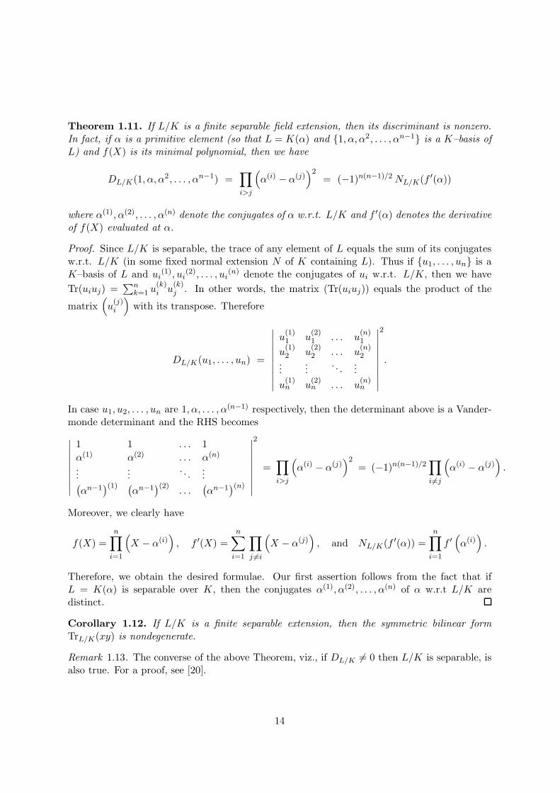
Theorem 1.11. If L/K is a finite separable field extension, then its discriminant is nonzero.In fact, if α is a primitive element (so that L = K(α) and 1, α, α2, . . . , αn−1 is a K–basis ofL) and f(X) is its minimal polynomial, then we have

DL/K(1, α, α2, . . . , αn−1) =∏

i>j

(

α(i) − α(j))2

= (−1)n(n−1)/2 NL/K(f ′(α))

where α(1), α(2), . . . , α(n) denote the conjugates of α w.r.t. L/K and f ′(α) denotes the derivativeof f(X) evaluated at α.

Proof. Since L/K is separable, the trace of any element of L equals the sum of its conjugatesw.r.t. L/K (in some fixed normal extension N of K containing L). Thus if u1, . . . , un is aK–basis of L and ui

(1), ui(2), . . . , ui

(n) denote the conjugates of ui w.r.t. L/K, then we have

Tr(uiuj) =∑n

k=1 u(k)i u

(k)j . In other words, the matrix (Tr(uiuj)) equals the product of the

matrix(

u(j)i

)

with its transpose. Therefore

DL/K(u1, . . . , un) =

∣∣∣∣∣∣∣∣∣∣

u(1)1 u

(2)1 . . . u

(n)1

u(1)2 u

(2)2 . . . u

(n)2

......

. . ....

u(1)n u

(2)n . . . u

(n)n

∣∣∣∣∣∣∣∣∣∣

2

.

In case u1, u2, . . . , un are 1, α, . . . , α(n−1) respectively, then the determinant above is a Vander-monde determinant and the RHS becomes

∣∣∣∣∣∣∣∣∣

1 1 . . . 1

α(1) α(2) . . . α(n)

......

. . ....

(αn−1

)(1) (αn−1

)(2). . .

(αn−1

)(n)

∣∣∣∣∣∣∣∣∣

2

=∏

i>j

(

α(i) − α(j))2

= (−1)n(n−1)/2∏

i6=j

(

α(i) − α(j))

.

Moreover, we clearly have

f(X) =n∏

i=1

(

X − α(i))

, f ′(X) =n∑

i=1

∏

j 6=i

(

X − α(j))

, and NL/K(f ′(α)) =n∏

i=1

f ′(

α(i))

.

Therefore, we obtain the desired formulae. Our first assertion follows from the fact that ifL = K(α) is separable over K, then the conjugates α(1), α(2), . . . , α(n) of α w.r.t L/K aredistinct.

Corollary 1.12. If L/K is a finite separable extension, then the symmetric bilinear formTrL/K(xy) is nondegenerate.

Remark 1.13. The converse of the above Theorem, viz., if DL/K 6= 0 then L/K is separable, isalso true. For a proof, see [20].

14

Chapter 2

Ring Extensions

In this chapter, we review some basic facts from Ring Theory.

2.1 Basic Processes in Ring Theory

There are three basic processes in Algebra using which we can obtain a new ring from a givenring1. Let us discuss them briefly.

Polynomial Ring: Given a ring A, we can form the ring of all polynomials in n variables(say, X1, . . . ,Xn) with coefficients in A. This ring is denoted by A[X1, . . . ,Xn]. Elements ofA[X1, . . . ,Xn] look like

f =∑

ai1...inXi11 . . . Xin

n , ai1...in ∈ A,

where (i1, . . . , in) vary over a finite set of nonnegative integral n–tuples. A typical term (ex-cluding the coefficient), viz., Xi1

1 . . . Xinn , is called a monomial; its (usual) degree is i1 + · · ·+ in.

If f 6= 0, then the (total) degree of f is defined by deg f = maxi1 + · · · + in : ai1...in 6= 0.Usual convention is that deg 0 = −∞. A homogeneous polynomial of degree d in A[X1, . . . ,Xn]is simply a finite A–linear combination of monomials of degree d. The set of all homogeneouspolynomials of degree d is denoted by A[X1, . . . ,Xn]d. Note that any f ∈ A[X1, . . . ,Xn] canbe uniquely written as f = f0 + f1 + . . . , where fi ∈ A[X1, . . . ,Xn]i and fi = 0 for i > deg f ;we may call fi’s to be the homogeneous components of f . If f 6= 0 and d = deg f , then clearlyfd 6= 0 and f = f0 + f1 + · · · + fd.

Quotient Ring: That is, the residue class ring A/I obtained by ‘moding out’ an ideal Ifrom a ring A. This is same as taking a homomorphic image. Passing to A/I from A has theeffect of making I the null element. We have a natural surjective homomorphism q : A→ A/Igiven by q(x) = x + I for x ∈ A. There is a one-to-one correspondence between the ideals of Acontaining I and the ideals of A/I given by J 7→ q(J) = J/I and J ′ 7→ q−1(J ′).

Localization: That is, the ring of fractions S−1A of a ring A w.r.t. a multiplicativelyclosed (m. c.) subset S of A [i.e., a subset S of A such that 1 ∈ S and a, b ∈ S ⇒ ab ∈ S].Elements of S−1A are, essentially, fractions of the type a

s , where a ∈ A and s ∈ S; the notion

of equality in S−1A is understood as follows. as = b

t ⇔ u(at − bs) = 0, for some u ∈ S.

1here, and hereafter, by a ring we mean a commutative ring with identity.

15

Quite often, we consider S−1A when A is a domain and 0 /∈ S; in this case, the notion ofequality (or, if you like, equivalence) is simpler and more natural. Note that if A is a domainand S = A \ 0, then S−1A is nothing but the quotient field of A. Important instance oflocalization is when S = A \ p, where p is a prime ideal of A; in this case S−1A is customarilydenoted by Ap. Passing from A to Ap has the effect of making p into a maximal ideal thatconsists of all nonunits; indeed, Ap is a local ring [which means, a ring with a unique maximalideal] with pAp as its unique maximal ideal. In general, we have a natural homomorphismφ : A → S−1A defined by φ(x) = x

1 . This is injective if S consists of nonzerodivisors, and inthis case A may be regarded as a subring of S−1A. Given an ideal I of A, the ideal of S−1Agenerated by φ(I) is called the extension of I, and is denoted by IS−1A or by S−1I. For anideal J of S−1A, the inverse image φ−1(J) is an ideal of A and is called the contraction of Jto A. By abuse of language, the contraction of J is sometimes denoted by J ∩ A. We haveS−1(J ∩A) = J and S−1I ∩A ⊇ I, and the last inclusion can be strict. This implies that thereis a one-to-one correspondence between the ideals J of S−1A and the ideals I of A such thata ∈ A : as ∈ I for some s ∈ S = I. This, in particular, gives a one-to-one correspondencebetween the prime ideals of S−1A and the prime ideals P of A such that P ∩ S = ∅.Exercise 2.1. Show that localization commutes with taking homomorphic images. More pre-cisely, if I is an ideal of a ring A and S is a m. c. subset of A, then show that S−1A/S−1I isisomorphic to S−1(A/I), where S denotes the image of S in A/I.

Given ideals I1 and I2 in a ring A, their sum I1 + I2 = a1 + a2 : a1 ∈ I1, a2 ∈ I2, theirproduct I1I2 = ∑ aibi : ai ∈ I1, bi ∈ I2, and intersection I1 ∩ I2 are all ideals. Analogue ofdivision is given by the colon ideal (I1 : I2), which is defined to be the ideal a ∈ A : aI2 ⊆ I1.If I2 equals a principal ideal (x), then (I1 : I2) is often denoted simply by (I1 : x). The idealsI1 and I2 are said to be comaximal if I1 + I2 = A. We can also consider the radical of an idealI, which is defined by

√I = a ∈ A : an ∈ I for some n ≥ 1, and which is readily seen to be

an ideal (by Binomial Theorem!). One says that I is a radical ideal if√

I = I. Note that thenotions of sum and intersections of ideals extend easily to arbitrary families of ideals.

Exercise 2.2. Show that colon commutes with intersections. That is, if Ii is a family of idealsof a ring A, then for any ideal J of A, we have ∩(Ii : J) = (∩Ii : J). Further, if Ii is a finitefamily, then show that

√∩Ii = ∩√Ii. Give examples to show that these results do not hold(for finite families) if intersections are replaced by products.

A useful fact about ideals is the following. The case when the ring in question is Z isconsidered, for example, in Ch’in Chiu-Shao’s Mathematical Treatise in the year 1247.

Proposition 2.3 (Chinese Remainder Theorem). Let I1, I2, . . . , In be pairwise comaximalideals in a ring A (i.e., Ii + Ij = A for all i 6= j). Then:

(i) I1I2 . . . In = I1 ∩ I2 ∩ · · · ∩ In.

(ii) Given any x1, . . . , xn ∈ A, there exists x ∈ A such that x ≡ xj(mod Ij) for 1 ≤ j ≤ n.

(iii) The map x(mod I1I2 · · · In) 7→ (x(mod I1), . . . , x(mod In)) defines an isomorphism ofA/I1I2 . . . In onto the direct sum A/I1 ⊕A/I2 ⊕ · · · ⊕A/In.

Proof. (i) Clearly, I1I2 . . . In ⊆ I1 ∩ I2 ∩ · · · ∩ In. To prove the other inclusion, we induct on n.The case of n = 1 is trivial. Next, if n = 2, then we can find a1 ∈ I1 and a2 ∈ I2 such that

16

a1 + a2 = 1. Now, a ∈ I1 ∩ I2 implies that a = aa1 + aa2, and thus a ∈ I1I2. Finally, if n > 2,then as in (i), let J1 = I2 · · · In and note that I1 + J1 = A. Hence by induction hypothesis andthe case of two ideals, I1 ∩ I2 ∩ · · · ∩ In = I1 ∩ J1 = I1J1 = I1I2 · · · In.

(ii) Given any i ∈ 1, . . . , n, let Ji = I1 · · · Ii−1Ii+1 · · · In. Since Ii + Ij = A, we can findaij ∈ Ij such that aij ≡ 1(mod Ii), for all j 6= i. Let ai =

∏

j 6=i aij . Then ai ≡ 1(mod Ii) andai ∈ Ji. Thus Ii + Ji = A. Now, x = x1a1 + · · · + xnan satisfies x ≡ xj(mod Ij) for 1 ≤ j ≤ n.

(iii) The map x(mod I1I2 · · · In) 7→ (x(mod I1), . . . , x(mod In)) is clearly well-defined anda homomorphism. By (i), it is surjective and by (ii), it is injective.

Exercise 2.4. With I1, . . . , In and A as in Proposition 2.3, show that the map in (iii) inducesan isomorphism of (A/I1I2 . . . In)× onto the direct sum (A/I1)

× ⊕ (A/I2)× ⊕ · · · ⊕ (A/In)×.

Deduce that the Euler φ-function is multiplicative.

2.2 Noetherian Rings and Modules

A ring A is said to be noetherian if every ideal of A is finitely generated. It is easy to see thatthis condition equivalent to either of the two conditions below.

(i) (Ascending Chain Condition or a.c.c.) If I1, I2, . . . are ideals of A such that I1 ⊆ I2 ⊆ . . . ,then there exists m ≥ 1 such that In = Im for n ≥ m.

(ii) (Maximality Condition) Every nonempty set of ideals of A has a maximal element.

The class of noetherian rings has a special property that it is closed w.r.t. each of the threefundamental processes. Indeed, if A is a noetherian ring, then it is trivial to check that bothA/I and S−1A are noetherian, for any ideal I of A and any m. c. subset S of A; moreover, thefollowing basic result implies, using induction, that A[X1, . . . ,Xn] is also noetherian.

Theorem 2.5 (Hilbert Basis Theorem). If A is a noetherian ring, then so is A[X].

Proof. Let I be any ideal of A[X]. For 0 6= f ∈ I, let LC(f) denote the leading coefficientof f , and J = 0 ∪ LC(f) : f ∈ I, f 6= 0. Then J is an ideal of A and so we can findf1, . . . , fr ∈ I \ 0 such that J = (LC(f1), . . . ,LC(fr)). Let d = maxdeg fi : 1 ≤ i ≤ r. For0 ≤ i < d, let Ji = 0∪LC(f) : f ∈ I, deg f = i; then Ji is an ideal of A and so we can findfi1, . . . , firi ∈ I such that Ji = (LC(fi1), . . . ,LC(firi)). Now if I ′ is the ideal of A[X] generatedby f1, . . . , fr ∪ fij : 0 ≤ i < d, 1 ≤ j ≤ ri, then I ′ ⊆ I and for any 0 6= f ∈ I, there isf ′ ∈ I ′ such that deg(f − f ′) < deg f . Thus an inductive argument yields I = I ′.

A field as well as a PID (e.g., Z, the ring of integers) is clearly noetherian, and constructingfrom these, using combinations of the three fundamental processes, we obtain a rather inex-haustible source of examples of noetherian rings. Especially important among these are finitelygenerated algebras over a field or, more generally, over a noetherian ring. Let us recall therelevant definitions.

Definition 2.6. Let B be a ring and A be a subring of B. Given any b1, . . . , bn ∈ B, wedenote by A[b1, . . . , bn] the smallest subring of B containing A and the elements b1, . . . , bn.This subring consists of all polynomial expressions f(b1, . . . , bn) as f varies over A[X1, . . . ,Xn].We say that B is a finitely generated (f. g.) A–algebra or an A–algebra of finite type if there

17

exist b1, . . . , bn ∈ B such that B = A[b1, . . . , bn]. Finitely generated k–algebras, where k is afield, are sometimes called affine rings.

A module over a ring A or an A–module is simply a vector space except that the scalars comefrom the ring A instead of a field. Some examples of A–modules are: ideals I of A, quotientrings A/I, localizations S−1A, and f. g. A–algebras A[x1, . . . , xn]. The notions of submodules,quotient modules, direct sums of modules and isomorphism of modules are defined in an obviousfashion. The concept of localization (w.r.t. m. c. subsets of A) also carries to A–modules, andan analogue of the property in Exercise 2.1 can be verified easily. Direct sum of (isomorphic)copies of A is called a free A–module; An = A⊕ · · · ⊕A

︸ ︷︷ ︸

n times

is referred to as the free A–module of

rank n.

Let M be an A–module. Given submodules Mi of M , their sum

∑

Mi = ∑

xi : xi ∈Mi and all except finitely many xi’s are 0

and their intersection ∩Mi are also submodules of M . Products of submodules doesn’t makesense but the colon operation has an interesting and important counterpart. If M1,M2 aresubmodules of M , we define (M1 : M2) to be the ideal a ∈ A : aM2 ⊆ M1 of A. The ideal(0 : M) is called the annihilator of M and is denoted by Ann(M); for x ∈ M , we may writeAnn(x) for the ideal (0 : x), i.e., for Ann(Ax). Note that if I is an ideal of A, then Ann(A/I) = Iand if Ann(M) ⊇ I, then M may be regarded as an A/I–module. Let us also note that for anysubmodules M1,M2 of M , we always have the isomorphisms (M1 +M2)/M2 ≃M1/(M1 ∩M2),and, if M2 ⊆M1 and N is a submodule of M2, (M1/N)/(M2/N) ≃M1/M2.

We say that M is finitely generated (f. g.) or that M is a finite A–module if there existx1, . . . , xn ∈ M such that M = Ax1 + · · · + Axn. Note that in this case M is isomorphic to aquotient of An. We can, analogously, consider the a.c.c. for submodules of M , and in the caseit is satisfied, we call M to be noetherian. Observe that M is noetherian iff every submoduleof M is finitely generated. In general, if M is f. g., then a submodule of M needn’t be f. g., i.e.,M needn’t be noetherian. However, the following basic result assures that ‘most’ f. g. modulesare noetherian.

Lemma 2.7. Finitely generated modules over noetherian rings are noetherian.

Proof (Sketch). First note that given a submodule N of M , we have that M is noetherian iffboth N and M/N are noetherian. Use this and induction to show that if A is noetherian, thenso is An, and, hence, any of its quotient modules.

Another basic fact about modules is the following.

Lemma 2.8 (Nakayama’s Lemma). Let M be a f. g. A–module and I be an ideal of A suchthat IM = M . Then there exists a ∈ I such that (1− a)M = 0. In particular, if I 6= A and Ais a local ring, then M = 0.

Proof. Write M = Ax1 + · · · + Axn. Then xi =∑n

j=1 aijxj, for some aij ∈ I. Let d =det(δij − aij). Then d = 1− a, for some a ∈ I, and, by Cramer’s rule, dxj = 0 for all j.

18

2.3 Integral Extensions

The theory of algebraic field extensions has a useful analogue to ring extensions, which isdiscussed in this section.

Let B be a ring and A be a subring of B. We may express this by saying that B is a (ring)extension of A or that B is an overring of A.

Definition 2.9. An element x ∈ B is said to be integral over A if it satisfies a monic polynomialwith coefficients in A, i.e., xn + a1x

n−1 + · · ·+ an = 0 for some a1, . . . , an ∈ A. If every elementof B is integral over A, then we say that B is an integral extension of A or that B is integralover A.

Evidently, if x ∈ B satisfies an integral equation such as above, then 1, x, x2, . . . , xn−1

generate A[x] as an A–module. And if B′ is a subring of B containing A[x] such that B′ =Ax1 + · · · + Axn, then for any b ∈ B′, bxi =

∑aijxj for some aij ∈ A so that b satisfies the

monic polynomial det(Xδij − aij) ∈ A[X]. Thus we obtain the following criteria.

x ∈ B is integral over A ⇔ A[x] is a finite A–module

⇔ a subring B′ of B containing A[x] is a finite A–module.

In particular, if B is a finite A–module, then B is integral over A. The converse is true if wefurther assume (the necessary condition) that B is a f. g. A–algebra. This follows by observingthat the above criteria implies, using induction, that if x1, . . . , xn ∈ B are integral over A, thenA[x1, . . . , xn] is a finite A–module. This observation also shows that the elements of B whichare integral over A form a subring, say C, of B. If C = A, we say that A is integrally closed inB. A domain is called integrally closed or normal if it is integrally closed in its quotient field.Note that if S is a m. c. subset of A, B is integral over A, and J is an ideal of B, then S−1B(resp: B/J) is integral over S−1A (resp: A/J ∩ A); moreover, if A is a normal domain and0 /∈ S, then S−1A is also a normal domain.

Exercise 2.10. Show that a UFD is normal. Also show that if A is a domain, then A is normaliff A[X] is normal. Further, show that if A is a normal domain, K is its quotient field, and xis an element of a field extension L of K, then x is integral over A implies that the minimalpolynomial of x over K has its coefficients in A.

Example 2.11. Let B = k[X,Y ]/(Y −X2), and let x, y denote the images of X,Y in B so thatB = k[x, y]. Let A = k[y]. Then x is integral over A, and hence B is integral over A. On theother hand, if B = k[X,Y ]/(XY − 1) = k[x, y], then x is not integral over A = k[y]. It may beinstructive to note, indirectly, that B ≃ k[Y, 1/Y ] is not a finite k[Y ]–module. These examplescorrespond, roughly, to the fact that the projection of parabola along the x–axis onto the y–axis is a ‘finite’ map in the sense that the inverse image of every point is at ‘finite distance’,whereas in the case of hyperbola, this isn’t so. Similar examples in “higher dimensions” can beconstructed by considering projections of surfaces onto planes, solids onto 3–space, and so on.Examples of integral (resp: non–integral) extensions of Z are given by subrings B of algebraicnumber fields (viz., subfields of C of finite degree over Q) such that B ⊆ OK (resp: B 6⊆ OK),where OK denotes the ring of integers in K. Indeed, OK is nothing but the integral closure ofZ in K.

A precise definition of dimension for arbitrary rings can be given as follows.

19

Definition 2.12. The (Krull) dimension of a ring A is defined as

dim A = maxn : ∃ distinct primes p0, p1, . . . , pn of A such that p0 ⊂ p1 ⊂ · · · ⊂ pn.

Remark 2.13. Observe that a field has dimension 0. A PID which is not a field, in particularZ as well as k[X], is clearly of dimension 1. It can be proved that dim k[X1, . . . ,Xn] = n. Formore on this topic, see [1].

Some of the basic results about integral extensions are as follows. In the five results givenbelow, B denotes an integral extension of A and p denotes a prime ideal of A.

Theorem 2.14. A is a field if and only if B is a field. Also, if q is a prime ideal of B suchthat q∩A = p, then p is maximal iff q is maximal. Moreover, if q′ is any prime ideal of B suchthat q ⊂ q′ and q′ ∩A = p, then q = q′.

Corollary 2.15. dim B ≤ dim A. In particular, if B is a domain and dim A ≤ 1, thendim A = dim B.

Theorem 2.16 (Lying Over Theorem). There exists a prime ideal q of B such that q∩A = p.In particular, pB ∩A = p.

Theorem 2.17 (Going Up Theorem). If q is a prime ideal of B such that q∩A = p, and p′

is a prime ideal of A such that p ⊆ p′, then there exists a prime ideal q′ of B such that q ⊆ q′

and q′ ∩A = p.

Corollary 2.18. dim A = dim B.

Proofs (Sketch). Easy manipulations with integral equations of relevant elements proves thefirst assertion of Theorem 2.14; the second and third assertions follow from the first one bypassing to quotient rings and localizations respectively. To prove Theorem 2.16, consider A′ =Ap and B′ = S−1B where S = A \ p. Then B′ is an integral extension of A′ and if q′ is anymaximal ideal of B′, then q′∩A′ is necessarily maximal and thus q′∩A′ = pA′. Now q = q′ ∩Blies over p, and thus Theorem 2.16 is proved. Theorem 2.17 follows by applying Theorem 2.16to appropriate quotient rings.

Exercise 2.19. Prove the two corollaries above using the results preceding them.

Remark 2.20. It may be noted that Corollary 2.18 is an analogue of the simple fact that ifL/K is an algebraic extension of fields containing a common subfield k, then tr.deg.kL =tr.deg.kK. Recall that if K is a ring containing a field k, then elements θ1, . . . , θd of K are saidto be algebraically independent over k if they do not satisfy any algebraic relation over k, i.e.,f(θ1, . . . , θd) 6= 0 for any 0 6= f ∈ k[X1, . . . ,Xn]. A subset of K is algebraically independent ifevery finite collection of elements in it are algebraically independent. If K is a field then any twomaximal algebraically independent subsets have the same cardinality, called the transcendencedegree of K/k and denoted by tr.deg.kK; such subsets are then called transcendence basesof K/k; note that an algebraically independent subset S is a transcendence basis of K/k iffK is algebraic over k(S), the smallest subfield of K containing k and S. If B is a domaincontaining k and K is its quotient field, then one sets tr.deg.kB = tr.deg.kK. Finally, note thatk[X1, . . . ,Xn] and its quotient field k(X1, . . . ,Xn) are clearly of transcendence degree n over k.A good reference for this material is [20, Ch. 2].

20

2.4 Discriminant of a Number Field

In this section, we shall first discuss some basic properties of normal domains. A key resulthere is the so called Finiteness Theorem. This will lead to the notion of an integral basis andthe notion of absolute discriminant of a number field.

Proposition 2.21. Let A be a domain with K as its quotient field. Then we have the following.

(i) If an element α (in some extension L of K) is algebraic over K, then there exists c ∈ Asuch that c 6= 0 and cα is integral over A. Consequently, if α1, . . . , αn is a K–basis ofL, then there exists d ∈ A such that d 6= 0 and dα1, . . . , dαn is a K–basis of L whoseelements are integral over A.

(ii) If A is normal, and f(X), g(X) are monic polynomials in K[X] such that f(X)g(X) ∈A[X], then both f(X) and g(X) are in A[X].

(iii) If A is normal, L/K is a finite separable extension and α ∈ L is integral over A, thenthe coefficients of the minimal polynomial of α over K as well as the field polynomial ofα w.r.t. L/K are in A. In particular, TrL/K(α) ∈ A and NL/K(α) ∈ A, and moreover,if α1, . . . , an is a K–basis of L consisting of elements which are integral over A, thenDL/K(α1, . . . , αn) ∈ A.

Proof. (i) If α satisfies the monic polynomial Xn + a1Xn−1 + · · · + an ∈ K[X], then we can

find a common denominator c ∈ A such that c 6= 0 and ai = cic for some ci ∈ A. Multiplying

the above polynomial by cn, we get a monic polynomial in A[X] satisfied by cα.(ii) The roots of f(X) as well as g(X) (in some extension of K) are integral over A becausethey satisfy the monic polynomial f(X)g(X) ∈ A[X]. Now the coefficients of f(X) as well asg(X) are the elementary symmetric functions of their roots (up to a sign), and therefore theseare also integral over A. But the coefficients are in K. It follows that both f(X) and g(X) arein A[X].(iii) If α is integral over A, then clearly so is every conjugate of α w.r.t. L/K. Now an argumentsimilar to that in (ii) above shows that the coefficients of Irr(α,K) as well as the field polynomialof α w.r.t. L/K are in A.

It may be observed that a proof of the FACT in Section 1.2 follows from (ii) above. We arenow ready to prove the following important result.

Theorem 2.22 (Finiteness Theorem). Let A be a normal domain with quotient field K.Assume that L/K is a finite separable extension of degree n. Let B be the integral closure of Ain L. Then B is contained in a free A–module generated by n elements. In particular, if A isalso assumed to be noetherian, then B is a finite A–module and a noetherian ring.

Proof. In view of (i) in the Proposition above, we can find a K–basis α1, . . . , αn of L, whichis contained in B. Let β1, . . . , βn be a dual basis, w.r.t. the nondegenerate bilinear formTrL/K(xy), corresponding to α1, . . . , αn. Let x ∈ B. Then x =

∑

j bjβj for some bj ∈ K.Now Tr(αix) =

∑

j bjTr(αiβj) = bi. Moreover, since αix is integral over A, it follows from theProposition above that bi ∈ A. Thus B is contained in the A–module generated by β1, . . . , βn.This module is free since β1, . . . , βn are linearly independent over K.

21

When A is a PID, or better still, when A = Z, the conclusion of Finiteness Theorem can besharpened using the following lemma.

Lemma 2.23. Let A be a PID, M be an A–module generated by n elements x1, . . . , xn, andlet N be a submodule of M .

(i) N is generated by at most n elements. In fact, we can find aij ∈ A for 1 ≤ i ≤ j ≤ nsuch that

N = Ay1 + · · ·+ Ayn where yi =∑

j≥i

aijxj for 1 ≤ i ≤ n. (2.1)

(ii) Assume that A = Z and M is a Z-submodule of K, where K is a number field with[K : Q] = n. Further assume that N contains a Q-basis of K. Then M/N is finite andwe can choose aij ∈ A, for 1 ≤ i ≤ j ≤ n, satisfying (2.1) and with the additional property

aii > 0 for 1 ≤ i ≤ n and |M/N | = a11a22 · · · ann = det(aij) (2.2)

where, by convention, aij = 0 for j < i.

Proof. (i) We have M = Ax1 + · · · + Axn. Let us use induction on n. Let

I = a ∈ A : ax1 + a2x2 + · · · + anxn ∈ N for some a2, . . . , an ∈ A.

Then I is an ideal of A and thus I = (a11) for some a11 ∈ A. Also, there exist a12, . . . , a1n ∈ Asuch that y1 ∈ N where y1 = a11x1 + a12x2 + · · · + a1nxn. If n = 1, we have N = Ix1 = Ay1,where y1 = a11x1 and thus the result is proved in this case. If n > 1, then let M1 = Ax2+. . . Axn

and N1 = N ∩M1. By induction hypothesis, we can find aij ∈ A for 2 ≤ i ≤ j ≤ n such that

N1 = Ay2 + · · ·+ Ayn where yi =∑

j≥i

aijxj for 2 ≤ i ≤ n.

Now if y ∈ N , then y = a1x1 + a2x2 + · · ·+ anxn for some a1, . . . , an ∈ A. Moreover a1 ∈ I andthus a1 = λ1a11 for some λ1 ∈ A. Hence y− λ1y1 ∈ N1 and so y− λ1y1 = λ2y2 + · · ·+ λnyn forsome λ2, . . . , λn ∈ A. It follows that N = Ay1 + · · ·+ Ayn and yi =

∑

j≥i aijxj, as desired.(ii) To begin with, let aij ∈ A = Z and yi ∈ N be such that (2.1) holds. If N contains

a Q-basis of K, then it is clear that K = Qy1 + · · · + Qyn and hence y1, . . . , yn are linearlyindependent over Q. Now, if some aii = 0, then we see easily that yi is a Q-linear combinationof yi+1, . . . , yn, which is a contradiction. Thus, aii 6= 0 for 1 ≤ i ≤ n and so replacing some yi’sby −yi’s, if necessary, we can assume that aii > 0 for 1 ≤ i ≤ n.

Given any x ∈ M , write x = a1x1 + · · · + anxn, where a1, . . . , an ∈ Z. We can find uniqueintegers q1 and r1 such that a1 = a11q1 + r1 and 0 ≤ r1 < a11. Hence

x− q1y1 = r1x1 + b2x2 + · · · + bnxn for some b2, . . . , bn ∈ Z.

Next, let q2, r2 ∈ Z be such that b2 = a22q2 + r2 and 0 ≤ r2 < a22. Hence

x− q1y1 − q2y2 = r1x1 + r2x2 + c3x3 + · · ·+ cnxn for some c3, . . . , cn ∈ Z.

Continuing in this way, we obtain q1, . . . , qn ∈ Z and r1, . . . , rn ∈ Z such that

x− (q1y1 + · · · + qnyn) = r1x1 + · · ·+ rnxn with 0 ≤ ri < aii.

22

Thus r1x1 + · · · + rnxn is a representative of x in M/N . Moreover, this representative isunique because the difference of two such representatives will be an element of N of the forms1x1+· · ·+snxn, where si ∈ Z with |si| < aii, and from (2.1), one sees easily that if sj is the firstnonzero integer among s1, . . . , sn, then ajj divides sj, which is a contradiction. It follows thatthe elements of M/N are in bijection with n-tuples (r1, . . . , rn) of integers with 0 ≤ ri < aii.Consequently, |M/N | = a11a22 · · · ann.

Corollary 2.24. Let A,K,L, n,B be as in the Finiteness Theorem. Assume that A is aPID. Then B is a free A–module of rank n, i.e., there exist n linearly independent elementsy1, . . . , yn ∈ B such that B = Ay1 + · · · + Ayn.

Proof. Follows from Finiteness Theorem 2.22 and Lemma 2.23 (i).

The above Corollary applied in the particular case of A = Z, shows that the ring of integersof a number field always has a Z–basis. Such a basis is called an integral basis of that ring orof the corresponding number field.

In general, suppose K is a number field with [K : Q] = n, and N is a Z-submodule ofM = OK such that N contains a Q-basis of K. Then by Lemma 2.23 (ii), we see that N hasa Z-basis of n elements, and we call this an integral basis of N . Notice that if α1, . . . , αn isan integral basis of N ⊆ OK , then by Proposition 2.21 (iii), DL/K(α1, . . . , αn) is an integer.Further, if u1, . . . , un is any Q–basis of K contained in N , then ui =

∑

j aijαj for somen × n nonsingular matrix (aij) with entries in Z. If d = det(aij), then d ∈ Z and we haveDL/K(u1, . . . , un) = d2DL/K(α1, . . . , αn). If u1, . . . , un is also an integral basis of N , thenclearly d = ±1. It follows that any two integral bases of N have the same discriminant, andamong all bases of K contained in N , the discriminant of an integral basis has the least absolutevalue. We denote the discriminant of an integral basis of N by ∆(N) and call this the (absolute)discriminant of N . In case N = OK , the discriminant ∆(OK) is denoted by dK and called the(absolute) discriminant of K. The two discriminants ∆(N) and dK = ∆(OK) are related bythe formula

∆(N) = |OK/N |2dK , (2.3)

which is an immediate consequence of Lemmas 1.9 and 2.23 (ii) where in the latter we takex1, . . . , xn to be an integral basis of K.

There are two cases when the formula (2.3) is particularly useful. One is when K = Q(α)is generated by a single element α which is integral over Z and N = Z[α]. In this case, if weknow that ∆(Z[α]) = DK/Q(1, α, . . . , αn−1) is squarefree, then we can conclude from (2.3) thatOK = Z[α]. Another case is when N is a nonzero ideal I of OK . Note that I 6= 0 implies thatI ∩Z 6= 0 since A is integral over Z; now, if m is a nonzero integer in I ∩Z and α1, . . . , αn isa Q-basis of K contained in OK , then mα1, . . . ,mαn is a Q-basis of K contained in I. ThusI does satisfy the hypothesis for the existence of an integral basis and for the formula (2.3) tohold with N = I. This case will be taken up again in Chapter 4.

Remark 2.25. An alternative proof of the existence of an integral basis of K can be given bypicking a Q–basis of K contained in OK whose discriminant has the least possible absolutevalue, and showing that this has to be an integral basis. Try this! Or see Appendix B for aproof along these lines.

23

In general, if A is a normal domain with quotient field K, L/K is finite separable of degreen, and B is the integral closure of A in L, then instead of a single number such as dK , one hasto consider the ideal of A generated by the elements DL/K(α1, . . . , αn) as α1, . . . , αn varyover all K–bases of L which are contained in B; this ideal is called the discriminant ideal ofB/A or of L/K, and is denoted DB/A. In case A happens to be a PID (which is often the casein number theoretic applications), we can replace this ideal by a generator of it, which thenplays a role analogous to dK .

We now discuss two examples to illustrate the computation of discriminant and determina-tion of integral bases.

Example 1: Quadratic Fields.

Let K be a quadratic field and O be its ring of integers. As noted before, we have K =Q(√

m), where m is a squarefree integer. We now attempt to give a more concrete descriptionof O. First, note that Z[

√m] = r + s

√m : r, s ∈ Z ⊆ O. Let x = a + b

√m ∈ O for some

a, b ∈ Q. Then Tr(x) = 2a and N(x) = a2 − mb2 (verify!) and both of them must be in Z.Since m is squarefree and a2 −mb2 ∈ Z, we see that a ∈ Z if and only if b ∈ Z. Thus if a /∈ Z,then we can find an odd integer a1 such that 2a = a1, and relatively prime integers b1 and c1

with c1 > 1 such that b = b1c1

. Now

(a1 = 2a ∈ Z and a2 −mb2 ∈ Z

)⇒(4|c2

1a21 and c2

1|4mb21

)⇒ c1 = 2.

Hence b1 is odd and a21 −mb2

1 ≡ 0(mod 4). Also a1 is odd, and therefore, m ≡ 1(mod 4). Itfollows that if m 6≡ 1(mod 4), then a, b ∈ Z, and so in this case, O = a + b

√m : a, b ∈ Z and

1,√m is an integral basis. In the case m ≡ 1(mod 4), the preceding observations imply that

O ⊆

a1 + b1√

m

2: a1, b1 are integers having the same parity, i.e., a1 ≡ b1(mod 2)

and, moreover, 1+√

m2 ∈ O since it is a root of X2 − X − m−1

4 ; therefore O = Z[1+√

m2 ] and

1, 1+√

m2 is an integral basis. We can now compute the discriminant of K as follows.

dK =

det

(2 00 2m

)

= 4m if m ≡ 2, 3(mod 4)

det

(2 11 (1 + m)/2

)

= m if m ≡ 1(mod 4).

It may be remarked that the integer d = dK determines the quadratic field K completely, and

the set 1, d+√

d2 is always an integral basis of K. (Verify!)

Example 2: Cyclotomic Fields.

Let p be an odd prime and ζ = ζp be a primitive pth root of unity. Consider the cyclotomicfield K = Q(ζ). We know that K/Q is a Galois extension and its Galois group is isomorphicto (Z/pZ)×, which is cyclic of order p− 1. The minimal polynomial of ζ over Q is given by

Φp(X) =Xp − 1

X − 1= Xp−1 + Xp−2 + · · ·+ X + 1 =

p−1∏

i=1

(X − ζi

).

24

We now try to determine OK , the ring of integers of K, and dK , the discriminant of K. Let usfirst note that since ζ ∈ OK , the ring Z[ζ], which is generated as a Z–module by 1, ζ, ζ2, . . . , ζp−1,is clearly contained in OK . Moreover, we have

DK/Q(1, ζ, . . . , ζp−1) = (−1)(p−1)(p−2)/2NK/Q(Φ′p(ζ)) = (−1)(p−1)/2NK/Q

(pζp−1

(ζ − 1)

)

.

Since Φp(X) = Xp−1 + · · · + X + 1 is the minimal polynomial of ζ over Q, we clearly see thatNK/Q(ζ) = (−1)p−1 · 1 = 1. And since the minimal polynomial of ζ − 1 is

Φp(X + 1) =(X + 1)p − 1

X=

p∑

i=1

(p

i

)

Xi−1 = Xp−1 + pXp−2 + · · · +(

p

2

)

X + p,

we see that N(ζ − 1) = (−1)p−1p = p. Thus N(Φ′p(ζ)) = pp−1·1

p = pp−2. On the other hand,N(ζ − 1) is the product of its conjugates, and so we obtain the identity

p = (ζ − 1)(ζ2 − 1) . . . (ζp−1 − 1),

which implies that the ideal (ζ − 1)OK ∩ Z contains pZ. But (ζ − 1) is not a unit in OK (lestevery conjugate (ζi − 1) would be a unit and hence p would be a unit in Z). So it followsthat (ζ − 1)OK ∩ Z = pZ. Now suppose x ∈ OK . Then x = c0 + c1ζ + · · · + cp−1ζ

p−1

for some ci ∈ Q. We shall now show that ci are, in fact, in Z. To this effect, consider(ζ − 1)x = c0(ζ − 1) + c1(ζ

2 − ζ) + · · · + cp−1(ζp − ζp−1). We have Tr(ζ − 1) = −p and

Tr(ζi+1−ζi) = 1−1 = 0 for 1 ≤ i < p. Therefore c0p = −Tr((ζ−1)x) ∈ (ζ−1)OK∩Z = pZ, andso c0 ∈ Z. Next, ζ−1(x−c0) = ζp−1c0 is an element of OK which equals c1+c2ζ+ · · ·+cp−1ζ

p−2.Using the previous argument, we find that c1 ∈ Z. Continuing in this way, we see that ci ∈ Z

for 0 ≤ i ≤ p− 1. It follows that OK = Z[ζ] and 1, ζ, ζ2, . . . , ζp−1 is an integral basis of OK .As a consequence, we obtain that

dK = DK/Q(1, ζ, ζ2, . . . , ζp−1) = (−1)(p−1)/2pp−2.

Exercise 2.26. Let n = pe where p is a prime and e is a positive integer. Show that the ringof integers of Q(ζn) is Z[ζn] and the discriminant of Q(ζn) is equal to (−1)ϕ(p)/2ppe−1(pe−e−1).Deduce that, in particular, the only prime dividing this discriminant is p and that the sign ofthis discriminant is negative only if n = 4 or p ≡ 3(mod 4).

Remark 2.27. If n is any integer > 1 and ζ = ζn is a primitive nth root of unity, then itcan be shown that the ring of integers of Q(ζn) is Z[ζn] and the discriminant of Q(ζn) equals(−1)ϕ(n)/2nϕ(n)

∏

p|n p−ϕ(n)/(p−1). The proof is somewhat difficult. See [19] for details.

Exercise 2.28 (Stickelberger’s Theorem). If K is a number field, then dK ≡ 0 or 1(mod 4).

[Hint: Let u1, . . . , un be an integral basis of K so that dK =[

det(

u(j)i

)]2, where u

(1)i , . . . , u

(n)i

denote the conjugates of ui w.r.t. K/Q. Write the above determinant as P −N , where P andN denote the contribution from even and odd permutations, respectively. Show that P + Nand PN are integers and dK = (P + N)2 − 4PN .] Verify this congruence from the formulaeabove when K is a quadratic field or a cyclotomic field,

Exercise 2.29. Let K = Q(α) where α is a root of X3 + 2X + 1. Show that ∆(Z[α]) = −59.Deduce that 1, α, α2 is an integral basis of K.

25

Chapter 3

Dedekind Domains and Ramification

Theory

In the investigation of Fermat’s Last Theorem and Higher Reciprocity Laws, mathematiciansin the 19th century were led to ask if the unique factorization property enjoyed by the integersalso holds in the ring of integers in an algebraic number field, especially in the ring of cyclotomicintegers. In 1844, E. Kummer showed that this does not hold, in general. About three yearslater, he showed that the unique factorization in such rings, or at least in rings of cyclotomicintegers, is possible if numbers are replaced by the so called “ideal numbers”. Kummer’s workwas simplified and furthered by R. Dedekind1. The concept of an ideal in a ring was thusborn. In effect, Dedekind showed that the ring of integers of an algebraic number field has thefollowing property:

Every nonzero ideal in this ring factors uniquely as a product of prime ideals.

Integral domains with this property are now known as Dedekind domains (or also Dedekindrings)2. In a famous paper3, Emmy Noether gave a set of abstract axioms for rings whoseideal theory agrees with that of ring of integers of an algebraic number field. This leadsto a characterization of Dedekind domains. In the next section, we will take this abstractcharacterization as the definition of a Dedekind domain, and then prove properties such as

1Dedekind published his ideas as a supplement to Dirichlet’s lectures on Number Theory, which were firstpublished in 1863. Dedekind’s supplements occur in the third and fourth editions, published in 1879 and 1894, ofDirichlet’s Vorlesungen uber Zahlentheorie. Another approach towards understanding and extending the ideas ofKummer was developed by L. Kronecker, whose work was apparently completed in 1859 but was not publisheduntil 1882. For more historical details, see the article “The Genesis of Ideal Theory” by H. Edwards, publishedin Archives for History of Exact Sciences, Vol. 23 (1980), and the articles by P. Ribenboim and H. Edwards in“Number Theory Related to Fermat’s Last Theorem”, Birkhauser, 1982.

2The term Dedekind domains was coined by I.S. Cohen [Duke Math. J. 17 (1950), pp. 27–42]. In fact, Cohendefines a Dedekind domain to be an integral domain in which every nonzero proper ideals factors as a productof prime ideals, and he notes that the uniqueness of factorization is automatic, thanks to the work of Matusita[Japan J. Math. 19 (1944), pp. 97–110].

3Abstrakter Aufbau der Idealtheorie in algebraischen Zahlund Funktionenkorpern, Math. Ann. 96 (1927), pp.26–61. The Aufbau paper followed another famous paper Idealtheorie in Ringbereichen [Math. Ann. 83 (1921),pp. 24–66] in which rings with ascending chain condition on ideals are studied; the term noetherian rings forsuch rings was apparently originated by Chevalley [Ann. Math. 44 (1943), pp. 690–708]. Incidentally, EmmyNoether had a great appreciation of Dedekind’s work and her favorite expression to her students was Alles steht

schon bei Dedekind!

26

the unique factorization of ideals as a consequence. In the subsequent sections, we study thephenomenon of ramification and discuss a number of basic results concerning it.

3.1 Dedekind Domains

An integral domain A is called a Dedekind domain if A is noetherian, normal and every nonzeroprime ideal in A is maximal. Note that the last condition is equivalent to saying that dimA ≤ 1,or in other words, either A is a field or A is one dimensional.

Example 3.1. Any PID is a Dedekind domain (check!). In particular, Z and the polynomialring k[X] over a field k are Dedekind domains.

Example 3.2. The ring Z[√−5], which is the ring of integers of the quadratic field Q(

√−5) is

a Dedekind domain. Indeed, this ring is noetherian being the quotient of a polynomial ringover Z, it is normal being the ring of integers of a number field, and it is one dimensional,being an integral extension of Z. However, Z[

√−5] is not a PID because, for instance, the ideal

P = (2, 1+√−5) is not principal. Indeed if P were generated by a single element a+b

√−5, then

a would have to be an even integer which divides 1, and this is impossible. As it turns out, thefact that the Dedekind domain Z[

√−5] is not a PID is related to failure of unique factorization

in Z[√−5], which is illustrated by the two distinct factorizations 2×3 and (1+

√−5)(1−

√−5)

of the number 6. Note, however, that if we pass to ideals and consider the principal ideal (6)generated by 6 in Z[

√−5], then there is no problem because

(6) = (2, 1 +√−5)(2, 1 −

√−5)(3, 1 +

√−5)(3, 1 −

√−5)

and it can be seen that the ideals on the right are distinct prime ideals and the above factor-ization of (6) into prime ideals is unique up to rearrangement of factors.

Many more examples of Dedekind domains can be generated from the following basic result.

Theorem 3.3 (Extension Theorem). Let A be a Dedekind domain, K its quotient field, La finite separable extension of K, and B the integral closure of A in L. Then B is a Dedekinddomain.

Proof. By Finiteness Theorem 2.22, B is noetherian. It is obvious that B is normal. Lastly, byCorollary 2.18 we see that dimB = dim A ≤ 1.

Since Z is a Dedekind domain, we obtain as an immediate consequence the following corol-lary.

Corollary 3.4. If K is a number field, then OK , the ring of integers of K, is a Dedekinddomain.

Exercise 3.5. Let A be a Dedekind domain with quotient field K. If S is any multiplicativelyclosed subset of A such that 0 /∈ S, then show that the localization S−1A of A at S is a Dedekinddomain with quotient field K. Moreover, if L is an algebraic extension of K, then show thatthe integral closure of S−1A in L is S−1B.

We shall now proceed to prove a number of basic properties of a Dedekind domain. Inparticular, we shall establish the fact about unique factorization of ideals as products of primeideals, which was alluded to in the beginning of this section.

27

Definition 3.6. Let A be a domain and K be its quotient field. By a fractionary ideal of A wemean an A-submodule J of K such that dJ ⊆ A for some d ∈ A, d 6= 0.

Note that a finitely generated A–submodule of K is a fractionary ideal of A. Conversely, ifA is noetherian, then every fractionary ideal of A is finitely generated.

To distinguish from fractionary ideals, the (usual) ideals of A are sometimes called theintegral ideals of A. Products of fractionary ideals is defined in the same way as the product ofintegral ideals, and w.r.t. this product, the set

FA = J : J a fractionary ideal of A and J 6= (0)

of all nonzero fractionary ideals is a commutative monoid with A as its identity element. Notethat FA contains the subset of nonzero principal fractionary ideals, viz.,

PA = Ax : x ∈ K, and x 6= (0)

and this subset is, in fact, a group. In case A is a PID, we see easily (from Corollary 2.24, forexample) that FA = PA, and in this case FA is a group. We will soon show that more generally,if A is any Dedekind domain, then FA is a group.

Lemma 3.7. Every nonzero ideal of a noetherian ring A contains a finite product of nonzeroprime ideals of A.

Proof. Assume the contrary. Then the family of nonzero nonunit ideals of A not containinga finite product of nonzero prime ideals of A is nonempty. Let I be a maximal element ofthis family. Then I 6= A and I can not be prime. Hence there exist a, b ∈ A \ I such thatab ∈ I. Now I + Aa and I + Ab are ideals strictly larger than I, and I ⊇ (I + Aa)(I + Ab).In particular, I + Aa and I + Ab are nonzero nonunit ideals. So by the maximality of I, bothI + Aa and I + Ab contain a finite product of nonzero prime ideals, and hence so does I. Thisis a contradiction.

Lemma 3.8. Let A be a noetherian normal domain and K be its quotient field. If x ∈ K andI is a nonzero ideal of A such that xI ⊆ I, then x ∈ A.

Proof. Since xI ⊆ I, we have xnI ⊆ I for n ≥ 1. Thus if we let J = A[x], then JI ⊆ I.In particular, if d ∈ I, d 6= 0, then dJ ⊆ A. So J is a fractionary ideal of A and since A isnoetherian, J = A[x] is a f.g. A-module. Therefore, x is integral over A and since A is normal,x ∈ A.

Lemma 3.9. Let A be a Dedekind domain and K be its quotient field. If P is any nonzeroprime ideal of A, then

P ′ = (A :K P ) = x ∈ K : xP ⊆ Ais a fractionary ideal of A, which strictly contains A. Moreover, PP ′ = A = P ′P . In particular,P is invertible and P−1 = P ′.

Proof. Clearly, P ′ is an A-module. Also, dP ′ ⊆ A for any d ∈ P , d 6= 0. Thus P ′ is afractional ideal of A. It is clear that P ′ ⊇ A. To show that P ′ 6= A, choose any d ∈ P , d 6= 0.By Lemma 3.7, we can find nonzero prime ideals P1, . . . , Pn of A such that (d) ⊇ P1 · · ·Pn.

28

Suppose n is the least positive integer with this property. Now, P1 · · ·Pn ⊆ P , and since Pis prime, we have Pi ⊆ P for some i. But A is a 1-dimensional ring, and so Pi = P . DefineI = P1 · · ·Pi−1Pi+1 · · ·Pn (note that I = A if n = 1). Then by the minimality of n, I 6⊆ (d). Letc ∈ I be such that c 6∈ (d). Then cd−1 6∈ A. But PI ⊆ (d), and this implies that P (c) ⊆ (d), andso cd−1 ∈ P ′. Thus P ′ 6= A. Next, to show that PP ′ = A, observe that P = PA ⊆ PP ′ ⊆ A.Thus PP ′ is an (integral) ideal of A containing the maximal ideal P . Hence PP ′ = A orPP ′ = P . But if x ∈ P ′ \A, then by Lemma 3.8, xP 6⊆ P , and hence PP ′ 6= P . It follows thatPP ′ = A.

Theorem 3.10. If A is a Dedekind domain, then FA, the set of nonzero fractionary ideals ofA, forms an abelian group (w.r.t products of fractionary ideals).

Proof. It suffices to show that every nonzero (integral) ideal of A is invertible, because if J ∈ FA,then dJ is a nonzero ideal of A for some d ∈ A, d 6= 0, and (d)(dJ)−1 is then the inverse of J .

Now if some nonzero ideal of A is not invertible, then we can find a nonzero ideal I ofA, which is not invertible and which is maximal with this property. Clearly I 6= A and sothere is a nonzero prime ideal P of A such that I ⊆ P . By Lemma 3.9, P−1 exists andI = IA ⊆ IP−1 ⊆ PP−1 = A. Moreover, if I = IP−1, then by Lemma 3.8, P−1 ⊆ A, whichcontradicts Lemma 3.9. Thus IP−1 is an ideal of A which is strictly larger than I. So bythe maximality of I, the ideal IP−1 is invertible. But then so is I = (IP−1)P . This is acontradiction.

Theorem 3.11. Let A be a Dedekind domain. Then every nonzero ideal I of A can be factoredas a product of prime ideals, and this factorization is unique up to a rearrangement of thefactors. More generally, every nonzero fractional ideal J of A factors as J = p

e11 · · · peh

h , forsome nonnegative integer h, distinct prime ideals p1, . . . , ph and nonzero integers e1, . . . , eh.

4

Furthermore, the prime ideals p1, . . . , ph and the corresponding exponents e1, . . . , eh are uniquelydetermined by J .

Proof. Assume for a moment that the assertion for integral ideals is proved. Then for anyJ ∈ FA, there exists d ∈ A, d 6= 0 such that dJ is a nonzero ideal of A. Now if dJ = p1 · · · pk

and (d) = q1 · · · ql, where pi and qj are prime ideals then J = p1 · · · pkq−11 · · · q−1

l . Moreover,if we also have J = P1 · · ·PmQ−1

1 · · ·Q−1n for some prime ideals Pi and Qj (necessarily nonzero

but not necessarily distinct), then p1 · · · pkQ1 · · ·Qn = q1 · · · qlP1 · · ·Pm and the uniqueness forfactorization of integral ideals can be used. This yields the desired results for nonzero fractionalideals.

To prove the existence of factorization of nonzero ideals of A into prime ideals, we canproceed as in the proof of Theorem 3.10. Thus, let I be a nonzero ideal of A which can not befactored as a product of prime ideals and which is maximal with this property. Then I 6= A andif P is a nonzero prime ideal containing I, then IP−1 is an ideal of A which is strictly largerthan I. So by the maximality of I, the ideal IP−1 is a product of prime ideals. Multiplying onthe right by P , we find that I is also a product of prime ideals. This is a contradiction.

To prove the uniqueness, let I be any nonzero ideal of A and suppose I = p1 · · · pr for somer ≥ 0 and prime ideals p1, . . . , pr. We induct on r to show that any other factorization of I as

4As per usual conventions, p−m =

(p−1)m

, for any positive integer m. Also, when h = 0, a product such asp

e11 · · · p

eh

h is the empty product and it equals (1) = A.

29

a product of prime ideals differs from p1 · · · pr by a rearrangement of factors. If r = 0, this isevident since a nonempty product of prime ideals will be contained in any one of the factors,which is a proper subset of A. Assume that r ≥ 1 and the result holds for ideals which areproducts of r − 1 prime ideals. Now if I = q1 · · · qs for some s ≥ 0 and prime ideals q1, . . . , qs,then it is clear that s > 0. Moreover, q1 · · · qs ⊆ p1 implies that qj ⊆ p1 for some j. But sinceI 6= (0), each qj is a nonzero prime ideal and hence maximal. Thus qj = p1. Multiplying I byp−11 we find that p2 · · · pr = q1 · · · qj−1qj+1 · · · qs. Thus by induction hypothesis r − 1 = s − 1

and p2, . . . pr are the same as q1, . . . , qj−1, qj+1, . . . , qs after a rearrangement. This implies thatr = s and p1, . . . , pr equal q1, . . . , qs after a rearrangement.

Remark 3.12. Either of the following four conditions can be taken as a definition for an integraldomain A to be a Dedekind domain.

(1) A is noetherian, normal and every nonzero prime ideal of A is maximal.

(2) Nonzero fractional ideals of A form a group with respect to multiplication.

(3) Every nonzero ideal of A factors uniquely as a product of prime ideals.

(4) Every nonzero ideal of A factors as a product of prime ideals.

Note that (3) ⇒ (4) is obvious and from Theorems 3.10 and 3.11, we have (1) ⇒ (2) and(1) ⇒ (3). Moreover, if (2) holds, then A is noetherian because if I is a nonzero ideal ofA, then II−1 = A implies that

∑ni=1 aibi = 1 for some ai ∈ I, bi ∈ I−1, and consequently,

I = (a1, . . . , an). Further, if (2) holds, then as in the proof of Theorem 3.11, the existenceof a nonzero ideal of A which can not be factored as a product of prime ideals leads to acontradiction. This shows that (2) ⇒ (4). Hence, to prove the equivalence of (1), (2), (3) and(4) it suffice to show that (4) ⇒ (1). This can be done but it needs a little bit of work; fordetails, we refer to [20, Ch. V, §6].Exercise 3.13. Use Theorem 3.11 to show that for every nonzero prime ideal p of A, we candefine a function np : FA → Z such that for any J ∈ FA, we have np(J) = 0 for all exceptfinitely many p, and

J =∏

p

pnp(J)

where the product is over all nonzero prime ideals p of A. Further show that J is an integral idealof A if and only if np(J) ≥ 0 for all nonzero prime ideals p of A. Deduce that for J1, J2 ∈ FA,

J1 ⊆ J2 ⇐⇒ np(J1) ≥ np(J2) for all nonzero prime ideals p of A.

Use this to show that if I1, I2 are integral ideals of A, then I1 ⊆ I2 if and only if I2 divides I1,i.e., I1 = I2I3 for some integral ideal I3 of A. Finally, for any J1, J2 ∈ FA and a nonzero primeideal p of A, prove the following.

(i) np(J1J2) = np(J1) + np(J2) and np(J1J−12 ) = np(J1)− np(J2).

(ii) np(J1 + J2) = min np(J1), np(J2) and np(J1 ∩ J)2 = max np(J1), np(J2).

30

We have seen in Example 3.2 that a Dedekind domain need not be a UFD. On the otherhand, if a Dedekind domain A is a UFD and P is any nonzero prime ideal of A, then P mustcontain an irreducible element because otherwise there will be an infinite strictly ascendingchain (a1) ⊂ (a2) ⊂ · · · of principal ideals contained in P , contradicting that A is noetherian.Now if p ∈ P is irreducible, then (p) is a nonzero prime ideal, and hence maximal. Hence,P = (p). Next, by Theorem 3.11, every nonzero ideal of A is a product of prime ideals andtherefore, it is principal. Thus A is a PID. Consequently, if a Dedekind domain A is a UFD,then FA = PA or in other words, the quotient group FA/PA is trivial.

Definition 3.14. Let A be a Dedekind domain and K be its quotient field. The ideal class groupof A, denoted by CA, is defined to be the quotient FA/PA. When K is a number field andA = OK is its ring of integers, CA is often denoted by CK and called the ideal class group of K.The elements of CK are called the ideal classes of K.

As remarked earlier, if A is a Dedekind domain, then

A is a UFD ⇐⇒ A is a PID ⇐⇒ CA is trivial.

Thus the size of the ideal class group CA is a measure of how far A is from being a UFD. In thecase when K is a number field and A = OK , it turns out that CK is a finite (abelian) group.The order of this group is denoted by hK and is called the class number of K. The finiteness ofclass number will be proved in Chapter 4 using some general results of Minkowski. A shorterproof is outlined in Exercise 4.3.

We end this section with a result which gives a sufficient condition for a Dedekind domainto be a PID.

Proposition 3.15. A local Dedekind domain is a PID. More generally, if a Dedekind domainhas only finitely many maximal ideals, then it is a PID.

Proof. Let A be a Dedekind domain with only finitely many maximal ideals, say, P1, . . . , Pr.Note that the ideals P1, . . . , Pr, and more generally, their powers Pm1

1 , . . . , Pmrr are pairwise

comaximal. Fix any i ∈ 1, . . . , r. Note that Pi 6= P 2i (because otherwise Pi = A). So we can

find ai ∈ Pi \ P 2i . By Chinese Remainder Theorem [cf. Prop. 2.3], there exists a ∈ A such that

a ≡ ai(mod P 2i ) and a ≡ 1(mod Pj) for 1 ≤ j ≤ r, j 6= i.

Now, (a) is a nonzero ideal of A with (a) ⊆ Pi, and the factorization of (a) into prime idealscan neither contain Pj for any j 6= i nor can it contain a power of Pi with exponent 2 or more.Hence (a) = Pi. Since every nonzero ideal of A is a product of the Pi’s, it must be principal.Thus A is a PID.

Remark 3.16. A ring with only finitely many maximal ideals is sometimes called a semilocalring. Thus the above Proposition says that a semilocal Dedekind domain is a PID. In the caseof local Dedekind domains, we can, in fact, say more. Namely, a local Dedekind domain is whatis called a discrete valuation ring or a DVR. An integral domain A with quotient field K is adiscrete valuation ring if there exists a map v : K \ 0 → Z with the properties

v(xy) = v(x) + v(y) and v(x + y) ≥ minv(x), v(y) for all x, y ∈ K \ 0

31

and A = x ∈ K : x = 0 or v(x) ≥ 0. The map v is called a valuation of K and A is calledits valuation ring. In case A is a local Dedekind domain, A has only one nonzero prime ideal,i say P , and for any nonzero element x of the quotient field of A, we can write Ax = Pn for aunique integer n, and the map given by x 7→ n is a valuation of K whose valuation ring is A.

Exercise 3.17. Let A be a Dedekind domain. If P is a nonzero prime ideal of A and e a positiveinteger, then show that A/P e is a principal ideal ring. Use this and the Chinese RemainderTheorem to show that if I is any nonzero ideal of A, then R/I is a principal ideal ring. Deducethat every ideal of A can be generated by two elements.

3.2 Extensions of Primes

In the ring OK of integers of a number field K, a prime p of Z may not remain a prime. Forinstance in the ring of integers of Q(

√−1), namely, in the ring Z[i] 5, the rational primes 2 and

5 are no longer primes but 3 is. However, by Theorem 3.11, the ideal generated by p in this ringcan be uniquely factored as a product of prime ideals. Roughly speaking, the phenomenon ofa prime splitting into several primes in an extension, is known as ramification. In this context,there is a beautiful analogue of the formula

∑gi=1 eifi = n, which holds when a monic polynomial

f(X) of degree n with coefficients in a field F , factors as f(X) = p1(X)e1 · · · pg(X)eg , whereg ≥ 0, ei > 0 and pi(X) are distinct monic irreducible polynomials in F [X] of degree fi. We nowproceed to give some relevant definitions and prove the

∑gi=1 eifi = n formula in the general

setting of Dedekind domains.

In this section, we shall assume that A,K,L,B are as in the Extension Theorem 3.3. Wewill also let n denote the degree of L/K.

Definition 3.18. Let p be a prime ideal of A. A prime ideal P of B is said to lie over p ifP ∩A = p.

Since B is a Dedekind domain, for any nonzero prime ideal p of A, the extension pB of p

to B is a nonzero ideal of B and hence it can be uniquely written as

pB =

g∏

i=1

P eii

where P1, P2, . . . , Pg are distinct nonzero prime ideals of B and ei are positive integers.

Exercise 3.19. With p and Pi as above, show that a prime ideal P of B lies over p iff P = Pi

for some i. Also show that pB ∩ A = p = P eii ∩ A. Deduce that B/pB as well as B/P ei

i B canbe regarded as vector spaces over the field A/p. Further show that B/Pi is a field extension ofA/p whose degree is at most n.

Definition 3.20. With p, Pi, etc. as above, the positive integer ei is called the ramificationindex of Pi over p and is denoted by e(Pi/p); the field degree [B/Pi : A/p] is called the residuedegree (or the residue class degree) of Pi over p and is denoted by f(Pi/p). If ei > 1 for some

5Elements of Z[i] are often called the Gaussian integers. These were first studied by C. F. Gauss in his workon biquadratic reciprocity.

32

i, then we say that p is ramified in B (or in L). Otherwise, it is said to be unramified. 6 Theextension L/K is said to be unramified if every nonzero prime ideal of A is unramified in L.

Exercise 3.21. Let A,K,L,B and p be as above. Suppose L′ is a finite separable extension ofL and B′ is the integral closures of B in L′. Show that B′ is the integral closure of A in L′.Further, if P a prime of B lying over p and P ′ a prime of B′ lying over P , then show that P ′

lies over p and the following transitivity relations hold:

e(P ′/p) = e(P ′/P )e(P/p) and f(P ′/p) = f(P ′/P )f(P/p).

We are now ready to prove the main result of this section.

Theorem 3.22. Let A,K,L,B be as above and n = [L : K]. Suppose p is a nonzero primeideal of A and we have

pB =

g∏

i=1

P eii

where P1, P2, . . . , Pg are distinct prime ideals of B and e1, . . . , eg are positive integers. Then,upon letting fi = [B/Pi : A/p], we have

g∑

i=1

eifi = n.

Proof. Let S = A \ p and A′ = S−1A be the localization of A at p. Then B′ = S−1B is theintegral closure of A′ in L, and pB′ = P ′

1e1 . . . P ′

geg , where P ′

i = PiB′. Moreover, the primes

P ′1, . . . , P

′g are distinct, A′/pA′ ≃ A/p and B′/P ′

i ≃ B/Pi. Thus we see that in order to provethe equality

∑eifi = n, we can replace A,B, p, Pi by A′, B′, p′, P ′

i respectively.

In view of the observations above, we shall assume without loss of generality that A is alocal Dedekind domain with p as its unique nonzero prime ideal. Then, by the Corollary 2.24,B is a free A–module of rank n = [L : K]. Write B = Ay1 + · · · + Ayn, where y1, . . . , yn aresome elements of B. Now for the vector space B/pB over A/p, we clearly have

B/pB =n∑

i=1

(A/p) yi

where yi denotes the residue class of yi mod pB. Moreover,

∑

aiyi = 0 =⇒∑

aiyi ∈ pB =⇒ ai ∈ p

where ai ∈ A and ai denotes its residue class mod p, and the last implication follows sincey1, . . . , yn is a free A–basis of B. It follows that y1, . . . , yn are linearly independent over A/p,and hence

dimA/p B/pB = n.

6To be accurate, we should define p to be ramified if ei > 1 for some i or B/Pi is inseparable over A/p for somei. However, in number theoretic applications, A/p will usually be a finite field and so the question of separabilityof residue field extensions doesn’t arise.

33

Now we count the same dimension by a different method. First, note that since P1, . . . , Pg

are distinct maximal ideals, P e11 , . . . , P

egg are pairwise comaximal. Since pB = P e1

1 · · ·Pegg , by

Chinese Remainder Theorem, we get an isomorphism (of rings as well as of (A/p)–vector spaces)

B/pB ≃g⊕

i=1

B/P eii .

Now let us find the dimension of the A/p–vector space B/P e where P = Pi and e = ei for somei. First, we note that for any j ≥ 1, pP j ⊆ P j+1, and hence P j/P j+1 can be considered as avector space over A/p. We claim that we have an isomorphism

B/P e ≃ B/P ⊕ P/P 2 ⊕ · · · ⊕ P e−1/P e.

To see this, use induction on e and the fact that for e > 1, we clearly have

B/P e−1 ≃ B/P e

P e−1/P e.

Next, we note that B is a Dedekind domain having only finitely many prime ideals (in fact, (0)and P1, . . . , Pg are the only primes of B), and so B must be a PID. Let t be a generator of P ,and consider the map

B/P → P j/P j+1

induced by the multiplication map x 7→ tjx of B → P j . This map is an A/p–homomorphism,and it is clearly bijective. So

dimA/p(Pj/P j+1) = dimA/p(B/P ) = f(P/p)

and consequently, from the above direct sum representations, we get

dimA/p(B/pB) =

g∑

i=1

dimA/p(B/P eii ) =

g∑

i=1

eifi,

which yields the desired identity. This completes the proof.

Examples:

1. Consider the quadratic field K = Q(i), where i denotes a square root of −1. We knowthat OK is the ring Z[i] of Gaussian integers. If p is a prime ≡ 1(mod 4), then we know (bya classical result of Fermat) that p can be written as a sum of two squares. Thus there exista, b ∈ Z such that p = a2 + b2 = (a + bi)(a − bi). It can be seen that (a + bi) and (a− bi) aredistinct prime ideals in OK . Thus for the prime ideal pZ, we have g = 2, e1 = e2 = 1 and (since∑

eifi = 2) f1 = f2 = 1. On the other hand, it is not difficult to see that a prime ≡ 3(mod 4)generates a prime ideal in Z[i] and so for such a prime, we have g = 1 = e1 and f1 = 2. Thecase of p = 2 is special. We have 2 = (1 + i)(1− i). But (1 + i) and (1− i) differ only by a unit(namely, −i) and thus they generate the same prime ideal. So 2 is a ramified prime and for it,we have g = 1 = f1 and e1 = 2.

34

2. In Example 2 of Section 2.4, where we discussed the pth cyclotomic field K = Q(ζp), wehave proved the identity

p = (ζ − 1)(ζ2 − 1) . . . (ζp−1 − 1),

and also the fact that (ζ−1)OK ∩Z = pZ. We note that for any integer i not divisible by p, wecan find an integer j such that ij ≡ 1(mod p), and thus (ζ i−1)/(ζ−1) = 1+ζ+· · ·+ζ i−1 ∈ Z[ζ]and its inverse (ζ − 1)/(ζi − 1) = (ζij − 1)/(ζi − 1) is also in Z[ζ]. Therefore, the fraction(ζi − 1)/(ζ − 1) is a unit in Z[ζ]. Consequently, (ζ i − 1) and (ζ − 1) generate the same ideal,say P . Now the above identity together with the previous Theorem shows that pZ[ζ] = P p−1

and P is a prime ideal. Thus we find that in this case g = 1 = f1 and e1 = p− 1 = [K : Q].

The last example illustrates the following definition.

Definition 3.23. A nonzero prime ideal p of A is said to be totally ramified in L (or in B) ifpB = Pn for some prime ideal P of B.

3.3 Kummer’s Theorem

In this section we prove a theorem, due to Kummer, which shows how the decomposition ofextended prime ideals can be “read off” from the factorization of a polynomial, for a certainclass of rings. It may be observed that the hypothesis of this theorem is satisfied in the case ofquadratic and cyclotomic extensions.

We shall use the following notation. Given a domain A and a maximal ideal p in A, we let A,denote the residue field A/p; for any polynomial p(X) ∈ A[X], by p(X) we denote its reductionmod p, i.e., the polynomial in A[X] whose coefficients are the p–residues of the correspondingcoefficients of p(X).

Theorem 3.24. Let A be a Dedekind domain, K its quotient field, L a finite separable extensionof K, and B the integral closure of A in L. Let p be a nonzero prime ideal of A. Assume thatB = A[α] for some α ∈ B. Let f(X) = Irr(α,K). Suppose

f(X) =

g∏

i=1

pi(X)ei

is the factorization of f(X) into powers of distinct monic irreducible polynomials in A[X]. Letpi(X) be the monic polynomial in A[X] whose reduction mod p is pi(X). Then the primes inB lying over p are precisely given by P1, . . . , Pg where Pi = pB + pi(α)B. Moreover,

pB =

g∏

i=1

P eii

is the factorization of pB into powers of distinct primes in B, the ramification index of Pi overp is the above exponent ei, and the residue degree fi of Pi over p is the degree of the irreduciblefactor pi(X).

Proof. Fix some i with 1 ≤ i ≤ g. Let αi be a root of pi(X). Consider the maps

A[X]→ A[X]→ A[X]/(pi(X)) ≃ A[αi]

35

where the first map sends a polynomial in A[X] to its reduction mod p, and the second one isthe natural quotient map. The composite of these maps is a homomorphism from A[X] ontoA[αi], and its kernel is clearly given by pA[X] + pi(X)A[X]. This kernel contains f(X), andthus we get the induced map of A[X]/(f(X)) onto A[αi]. Since B = A[α] ≃ A[X]/(f(X)),we get a map ϕi of B onto A[αi]. Note that ker ϕi is equal to pB + pi(α)B. Since pi(X) isirreducible in A[X], ker ϕi is a prime ideal in B which contains p. It is therefore a maximalideal in B lying over p. Also A is a field and

[B/ker ϕi : A/p] = dimA A[αi] = deg pi(X).

Now suppose P is any maximal ideal of B lying over p. Since

f(X)− p1(X)e1 . . . pg(X)eg ∈ pA[X]

and f(α) = 0, we see thatp1(α)e1 . . . pg(α)eg ∈ pB ⊆ P

and hence pi(α) ∈ P for some i, and then it follows that P must be equal to pB +pi(α)B. Thisshows that the primes lying in B over p are precisely P1, . . . , Pg where Pi = pB + pi(α)B, andthat the residue degree fi = f(Pi/p) equals deg pi(X). To prove the remaining assertion, let e′idenote the ramification index of Pi over p, so that

pB = Pe′11 . . . P

e′gg .

Since Pi = pB + pi(α)B, we have

P eii ⊆ pB + pi(α)eiB

and hence, in view of the above observation that p1(α)e1 . . . pg(α)eg ∈ pB, we have

P e11 . . . P

egg ⊆ pB + p1(α)e1 . . . pg(α)eg B ⊆ pB = P

e′11 . . . P

e′gg .

Consequently ei ≥ e′i for all i. But we know that

g∑

i=1

eifi = deg f(X) = [L : K] =

g∑

i=1

e′ifi.

Therefore ei = e′i for all i. This completes the proof.

Remark 3.25. If K is a number field, then by Primitive Element Theorem, there exists α ∈ Ksuch that K = Q(α). We can also choose this α to be in OK . However, a choice of α forwhich OK = Z[α] may not always be possible. In other words, the hypothesis of Kummer’sTheorem may not always be satisfied. As indicated earlier, quadratic fields and cyclotomicfields do satisfy the hypothesis of Kummer’s Theorem. Exercise 2.29 gives another example ofa number field K = Q(α) for which OK = Z[α]. On the other hand, the following exercise givesan example, due to Dedekind, of a number field K for which doesn’t satisfy the hypothesis ofKummer’s Theorem.

Exercise 3.26. Let α ∈ C be a root of X3 −X2 − 2X − 8 and K = Q(α). Prove the following:(i) [K : Q] = 3; (ii) if β = (α2 + α)/2, then β3 − 3β2 − 10β − 9 = 0, and hence β ∈ OK ; (iii)DK/Q(1, α, α2) = −4(503) and DK/Q(1, α, β) = −503, and hence 1, α, β is an integral basisof OK ; (iv) for any θ ∈ OK , DK/Q(1, θ, θ2) is an even integer; (v) OK 6= Z[θ] for any θ ∈ OK .

36

3.4 Dedekind’s Discriminant Theorem

Suppose we have a number field K whose ring of integers OK is of the form Z[α]. Let f(X) bethe minimal polynomial of α over Q and p be a rational prime7. Let f(X) ∈ Z/pZ[X] denotethe reduction of f(X) mod pZ. Then, by Kummer’s Theorem, p ramifies in K iff f(X) has amultiple root. Now, the polynomial f(X) has a multiple root iff its (classical) discriminant iszero (as an element of Z/pZ). The last condition means that DiscXf(X) = ±dK is divisible byp. Thus we find that in this situation we have:

p ramifies in K iff p divides dK .

In fact, this turns out to be true even in a more general situation. This section is devoted to aproof of this fundamental result, which is due to Dedekind.

Theorem 3.27. Let A be a Dedekind domain and K be its quotient field. Let L be a finiteseparable extension of K of degree n, and B be the integral closure of A in L. Let p be anonzero prime ideal of A. Assume that the field A/p is perfect (which means that every algebraicextension of this field is separable)8. Then we have:

p ramifies in L⇐⇒ p ⊇ DB/A.

In particular, if the above assumption on the residue field is satisfied by every nonzero primeideal of A, then there are only a finitely many prime ideals in A which ramify in L.

Proof. If we consider the localizations A′ = S−1A and B′ = S−1B where S = A \ p, then it isreadily seen that DB′/A′ = DB/AA′ and p ramifies in L iff p′ = pA′ ramifies in L. Thus to provethe first assertion, we can and will assume without loss of generality that A is a local Dedekinddomain and p is its unique maximal ideal.

Let pB = P e11 P e2

2 · · ·Pegg , where P1, P2, . . . , Pg are distinct prime ideals of B and e1, e2, . . . , eg

are their ramification indices. As noted in the proof of Theorem 3.22, we have pB ∩ A = p =P ei

i ∩A, and we have an isomorphism of A/p–vector spaces

B/pB ≃g⊕

i=1

B/P eii .

Let us set A = A/p and B = B/pB. For x ∈ B, let x denote the image of x in B. Note thatwe clearly have

TrB/A(x) = TrL/K(x) for all x ∈ B.

Now if α1, . . . , αn is any K–basis of L contained in B such that α1, . . . , αn is an A–basisof B, then using the above identity for traces, we see that

DB/A(α1, . . . , αn) = DL/K(α1, . . . , αn). (1)

7It is a common practice in Number Theory to call the usual primes as rational primes (and the usual integersas rational integers) so as to distinguish from primes (and integers) in the rings of integers of algebraic numberfields.

8This assumption would always be satisfied in number theoretic applications since A/p would usually be afinite field.

37

Next, we show that if B ≃ B1 ⊕ · · · ⊕ Bg, where the isomorphism is of A–vector spaces, thenwe have

DB/A =

g∏

i=1

DBi/A. (2)

To see the above identity, it suffices to consider the case when g = 2 since the general casewould follow by induction on g. For convenience of notation, let us denote the element of Bcorresponding to (u, 0) ∈ B1 ⊕ B2 by u itself and, similarly, the element of B corresponding to(0, v) ∈ B1⊕ B2 by v itself. It is clear that we can choose A–bases u1, . . . , ur and v1, . . . , vsof B1 and B2 respectively such that u1, . . . , ur, v1, . . . , vs is an A–basis of B. In view of theabove convention, we see that uivj = 0. Thus TrB/A(uivj) = 0, and so

DB/A(u1, . . . , ur, v1, . . . , vs) =

∣∣∣∣∣∣

Tr(uiui′) | 0. . . . . . | . . . . . .

0 | Tr(vjvj′)

∣∣∣∣∣∣

= DB1/A(u1, . . . , ur)DB2/A(v1, . . . , vs).

Since A is a field and the non-vanishing of any of the above discriminants is independent of thechoice of the corresponding A–bases, the desired equality of discriminant ideals follows. Thuswe have proved (2).

Now suppose p is a ramified prime. Then ei > 1 for some i and thus the ring B/P eii contains

a nonzero nilpotent element (which may be taken to be any element of P ei−1i \P ei

i ), and henceso does B. Let β ∈ B be such that β ∈ B is a nonzero nilpotent element. Extend β toan A–basis β1, . . . , βn of B with β1 = β. Since β1 is nilpotent, so is β1βj for 1 ≤ j ≤ n.Hence Tr(β1βj) = 0 for 1 ≤ j ≤ n [because if u ∈ B is nilpotent, then 0 is clearly the onlyeigenvalue of the linear transformation x 7→ ux of B → B and Tr(u) equals the sum of alleigenvalues of this linear transformation]. Consequently, DB/A(β1, . . . , βn) = 0, and so DB/A isthe zero ideal. Thus if α1, . . . , αn is an A–basis of B (which exists by Finiteness Theorem),then α1, . . . , αn is an A–basis of B and in view of (1), we see that DL/K(α1, . . . , αn) ∈ pB.It follows that DB/A ⊆ pB ∩A = p.

To prove the converse, assume that p ⊇ DB/A. Suppose, if possible, p is unramified. Thenei = 1 for all i and thus B is isomorphic (as an A–vector space) to the direct sum of the fieldsBi = B/Pi. Since A is perfect, the extension Bi/A is separable, and therefore DBi/A 6= 0, for1 ≤ i ≤ g. Thus by (2), we have DB/A 6= 0. But, in view of (1), this contradicts the assumptionthat DB/A ⊆ p. It follows that p must be a ramified prime.

The final assertion about the number of ramified prime is an immediate consequence of theabove characterization and the fact that DB/A is a nonzero ideal of the Dedekind domain A.

Corollary 3.28. Let K be a number field. A rational prime p ramifies in K iff p divides dK .In particular, only finitely many primes of Z ramify in K.

3.5 Ramification in Galois Extensions

In the case of Galois extensions, the fundamental identity∑

eifi = n, which was proved inSection 3.2, takes a particularly simple form. This short section is devoted to a proof of thissimpler identity. The key idea in the proof is the “norm argument” in the Lemma below.

38

Lemma 3.29. Let A be a normal domain, K its quotient field, L a Galois extension of K,B the integral closure of A, and p a prime ideal of A. Then the primes of B lying over p areconjugates of each other, i.e., for any prime ideals P,Q of B such that P ∩A = p = Q∩A, wehave Q = σ(P ) for some σ ∈ Gal(L/K). In particular, the number of prime ideals of B lyingover p is finite, and , in fact, ≤ [L : K].

Proof. We use a similar reduction as in the proof of Theorem 3.22. Thus we note that ifS = A \ p, then the integral closure of A′ = S−1A in L is B′ = S−1B, and PB′ and QB′ areprime ideals of B′ lying over pA′. Moreover if QB′ = σ(PB′), for some σ ∈ Gal(L/K), thenwe clearly have

Q = QB′ ∩B = σ(PB′) ∩B = σ(PB′) ∩ σ(B) = σ(PB′ ∩B) = σ(P ).

So we assume without loss of generality that p is a maximal ideal of A. Now since B/A isintegral, Q and P are maximal ideals of B. Suppose Q 6= σ(P ) for any σ ∈ Gal(L/K). ByChinese Remainder Theorem, we can find some x ∈ B such that

x ≡ 0(mod Q) and x ≡ 1(mod σ(P )) ∀σ ∈ Gal(L/K).

Consider the norm

NL/K(x) =∏

σ∈Gal(L/K)

σ(x).

By Proposition 2.21, this lies in A and hence in Q ∩ A = p. Now P is a prime ideal of Bcontaining p, and thus it follows that σ(x) ∈ P for some σ ∈ Gal(L/K). But this contradictsthe choice of x.

Corollary 3.30. Let A be a normal domain, K its quotient field, L a finite separable extensionof K, B the integral closure of A in L, and p a prime ideal in A. Then there exist only a finitenumber of prime ideals in B lying over p.

Proof. Let L′ be a least Galois extension of K containing L and B′ be the integral closure ofA in L′. Suppose P and Q are distinct prime ideals in B lying over p. Since B′ is integral overB, there exist prime ideals P ′ and Q′ in B′ lying over P and Q respectively. Clearly P ′ and Q′

are distinct and they both lie over p. Hence, by Lemma 3.29, we get the desired result.

Theorem 3.31. Let A be a Dedekind domain, K its quotient field, L a Galois extension of K,B the integral closure of A, and p a nonzero prime ideal of A. Then for the primes of B lyingover p, the ramification indices are the same and the residue degrees are the same. In otherwords, we have

pB = (P1P2 . . . Pg)e

where P1, . . . , Pg are distinct prime ideals of B, and f(P1/p) = · · · = f(Pg/p) (= f say).Moreover, if we let n = [L : K], then we have

efg = n.

39

Proof. Let pB = P e11 . . . P

egg , where P1, . . . , Pg are distinct prime ideals of B, and let fi =

f(Pi/p) for 1 ≤ i ≤ g. For any σ ∈ Gal(L/K), we clearly have σ(p) = p and σ(B) = B, andhence σ(pB) = pB. By Lemma 3.29, for any i with 1 ≤ i ≤ g, there exists σ ∈ Gal(L/K) suchthat σ(Pi) = P1, and consequently, B/Pi ≃ σ(B)/σ(Pi) = B/P1. Thus ei = e1 and fi = f1.Since we have already shown that

∑gi=1 eifi = n, the theorem follows.

Remark 3.32. With the notation and assumptions as in Theorem 3.31, we see that the ramifi-cation index e(P/p) of a prime P of B lying over p is independent of the choice of P . Thus itis sometimes denoted by ep. Likewise, in the case of Galois extensions, the notation fp and gp

is sometimes used.

3.6 Decomposition and Inertia Groups

The identity efg = n, proved in the last section, is a starting point of a beautiful theory oframification of primes developed by Hilbert. Some basic aspects of this theory will be discussedin this section. In order to avoid repetition, we state below the notations and assumptions thatwill be used throughout this section.

Notation and Assumption: Let A be a Dedekind domain and K be its quotient field.Let L be a Galois extension of K and B be the integral closure of A in L. Let G denote theGalois group of L/K. Let p be a nonzero prime ideal of A. Let A = A/p. Assume that A is aperfect field.9 Let e = ep, f = fp. and g = gp.

Observe that |G| = [L : K] = efg. Also note that if P is any prime of B lying over p, thenthe set primes of B lying over p is precisely σ(P ) : σ ∈ Gal(L/K). Thus the Galois group Gacts naturally on this set of g primes and the action is transitive.

Definition 3.33. Given any prime ideal P of B lying over p, the decomposition group of P w.r.t.L/K is defined to be the subgroup of G consisting of automorphisms σ such that σ(P ) = P . Itis denoted by DP (L/K) or simply by DP or D if the reference to L/K and/or P is clear fromthe context. The fixed field of DP (L/K) is called the decomposition field of P w.r.t. L/K, andis denoted by KD.

Note that DP (L/K) is the stabilizer of P for the natural action of G on the set of primesof B lying over p. Hence |DP (L/K)| = |G|/g = ef . Thus [L : KD] = ef and [KD : K] = g.Also note that if Q is any prime ideal of B lying over p, then Q = σ(P ) for some σ ∈ G, andwe have

τ ∈ DQ(L/K)⇔ τ(σ(P )) = σ(P )⇔ σ−1τσ ∈ DP (L/K)

and so DQ = σDP σ−1. Thus if DP is a normal subgroup of G (which, for example, is the caseif L/K is abelian), then it depends only on p and it may be denoted by Dp.

Lemma 3.34. Let P be a prime ideal of B lying over p, and D = DP (L/K) be its decompositiongroup. Let AD = B ∩KD be the integral closure of A in KD and let PD = P ∩AD. Then P isthe only prime of B lying over PD, and we have

PDB = P e and f(P/PD) = f.

9In number theoretic applications, A will usually be a finite field and thus this assumption is valid.

40

If D is a normal subgroup of G, then KD/K is a Galois extension and pAD is a product of gdistinct and conjugate primes of KD with residue degree 1.

Proof. Since L/KD is Galois, the set of primes of B lying over PD is given by σ(P ) : σ ∈Gal(L/KD) = P. Further, if e′ = e(P/PD) and f ′ = f(P/PD), then we know from Exercise3.21 that e′|e and f ′|f . On the other hand, e′f ′ = [L : KD] = ef . Hence e′ = e and f ′ = f .This proves our first assertion, and also it shows that e(PD/p) = 1 and f(PD/p) = 1. If D isnormal, then clearly KD/K is Galois and e(P ′/p) = 1 = f(P ′/p), for any prime P ′ of AD lyingover p. Since [KD : K] = g, we obtain the desired result.

For the remainder of this section, let us fix a prime P of B lying over p and let D =DP (L/K). Let B = B/P . Then B is a field extension of A of degree f . By our assumption,B/A is separable. Now if σ ∈ D, then σ clearly induces an A–automorphism σ of B. We thusobtain a homomorphism

ǫ : D → Gal(B/A) defined by ǫ(σ) = σ.

The kernel of ǫ is called the inertia group of P w.r.t. L/K and is denoted by TP (L/K) orsimply by TP or T . Clearly, T is a normal subgroup of D. Note that the inertia group can bealternatively defined as follows.

TP (L/K) = σ ∈ G : σ(x) = x(mod P ) for all x ∈ B.

The fixed field of T is called the inertia field of P w.r.t. L/K and is denoted by KT . Observethat K ⊂ KD ⊂ KT ⊂ L, and KT /KD is a Galois extension with Galois group D/T . A betterdescription of this group and its order is given by the following lemma.

Lemma 3.35. The extension B/A of residue fields is normal, and ǫ : D → Gal(B/A) definesan isomorphism of D/T onto Gal(B/A).

Proof. Let α ∈ B be any element, and α ∈ B be its representative. Let f(X) be the minimalpolynomial of α over K. Since α ∈ B, f(X) ∈ A[X]. Moreover, since L/K is normal, L andhence B contains all the roots of f(X). Now f(α) = 0 and thus Irr(α, A) divides f(X), thereduction of f(X) mod p. It follows that B contains all the roots of Irr(α, A). Thus B/A isnormal.

Next, we can find θ ∈ B such that B = A(θ) because B/A is a finite separable extension.Let θ ∈ B be a representative of B. By Chinese Remainder Theorem, we can find some β ∈ Bsuch that for any σ ∈ G we have

β ≡ θ(mod σ(P )) for σ ∈ D and β ≡ 0(mod σ(P )) for σ /∈ D.

Clearly β = θ and thus B = A(β). Let γ ∈ Gal(B/A) be any element. As in the previousparagraph, we see that γ(β) is the image of some conjugate of β. Thus γ(β) = σ(β) for someσ ∈ G. If σ /∈ D, then by the choice of β we have σ(β) ∈ P , i.e., γ(β) = σ(β) = 0, which isimpossible. It follows that γ = σ = ǫ(σ). This proves the Theorem.

41

Corollary 3.36. We have |T | = e = [L : KT ] and [KT : KD] = f . Further, if AT = B ∩KT isthe integral closure of A in KT and PT = P ∩AT , then we have

PDAT = PT with f(PT /PD) = f and PT B = P e with f(P/PT ) = 1.

In particular, we see that p is unramified in KT .

Proof. Since |D| = ef and [B : A] = f , it follows from Lemma 3.35 that |T | = e = [L : KT ]and [KT : KD] = f . Now if we consider the extension L/KT and the prime P lying over PT

(i.e., replace K,A, p by KT , AT , PT respectively), then we have DP (L/KT ) = TP (L/KT ) =Gal(L/KT ) = T and the above results show that e(P/PT ) = e and e(P/PT )f(P/PT ) = e.The desired result follows from this using the transitivity relations for ramification indices andresidue degrees.

Exercise 3.37. Let E be a subfield of L containing K and AE = B ∩ E be the integral closureof A in E. Let PE = P ∩ AE. Show that DP (L/E) = DP (L/K) ∩Gal(L/E) and TP (L/E) =TP (L/K) ∩Gal(L/E).

Exercise 3.38. Let H be the subgroup of G generated by the subgroups TP (L/K) as P variesover all nonzero prime ideals of B. Let E be the fixed field of H. Show that E/K is anunramified extension.

Exercise 3.39. For n ≥ 0, define Gn = σ ∈ G : σ(x) ≡ x(mod Pn+1). Show that Gn aresubgroups of G with G0 = T . Prove that Gn = 1 for all sufficiently large n. Also show thatG0/G1 is isomorphic to a subgroup of the multiplicative group of nonzero elements of B = B/P ,and therefore it is cyclic. Further show that for n ≥ 1, Gn/Gn+1 is isomorphic to a subgroupof the additive group B. Deduce that the inertia group T is a solvable group.

Remark 3.40. Let Kp be the completion of K w.r.t. the valuation of K corresponding top (whose valuation ring is Ap), and LP be the completion of L w.r.t. the valuation of Lcorresponding to P . Then we know that LP can be regarded as a field extension of Kp. Since Kp

is complete, there is only one prime of LP lying over the prime (or the corresponding valuation)of Kp. And since the residue fields of these primes in the completions coincide with the residuefields A and B respectively, it follows that the residue degrees are the same. Hence using theTheorem proved in the last section, we see that the ramification index corresponding to LP /Kp isprecisely e, and we have ef = [LP : Kp]. Moreover, every element of the decomposition groupD = DP (L/K) extends by continuity to an Kp–automorphism of LP , and since |D| = ef ,it follows that Gal(LP /Kp) ≃ DP (L/K). In particular, if P is unramified, then T = 1and thus D is isomorphic to Gal(B/A). Furthermore, if A is finite (which is the case if Kis a number field), then Gal(B/A) is cyclic, and thus whenever P is unramified, we haveGal(LP /Kp) ≃ Gal(B/A) ≃ Gal(LP /Kp), where LP and Kp denote the residue fields of (thevaluation rings of) LP and Kp respectively, so that the local Galois group Gal(LP /Kp) is cyclic.For more on these matters, see [17]

3.7 Quadratic and Cyclotomic Extensions

In this section we shall consider the examples of quadratic and cyclotomic fields and try todetermine explicitly the splitting of rational primes when extended to these number fields.

42

Example 1: Quadratic FieldsLet K be a quadratic field. As noted earlier, we have K = Q(

√m), for some uniquely

determined squarefree integer m (with m 6= 0, 1). Let O be the ring of integers of K. We havealso seen that

O =

Z[√

m] if m ≡ 2, 3(mod 4)

Z[1+√

m2 ] if m ≡ 1(mod 4).

In particular, we see that the hypothesis of Kummer’s Theorem 3.24 is satisfied.Now let p be a rational prime. We are interested in the decomposition of the extended ideal

pO. The formula∑g

i=1 eifi = n shows that g as well as ei, fi can only be 1 or 2, and that thesituation has to be one of the following.

(i) g = 2, e1 = f1 = e2 = f2 = 1 so that pO = P1P2 for some distinct primes P1, P2 of Owith O/Pi ≃ Z/pZ. In this case, we say that p is a decomposed (or split) prime, or that pdecomposes (or splits) in O.

(ii) g = 1, e1 = 2, f1 = 1 so that pO = P 2 for some prime P of O with O/P ≃ Z/pZ. Inthis case p is a ramified prime.

(iii) g = 1, e1 = 1, f1 = 2 so that pO = P for some prime P of O with [O/P : Z/pZ] = 2. Inthis case, we say that p is an inertial prime.

Now let’s figure out which one is which. First we consider

Case 1: m 6≡ 1(mod 4), i.e., m ≡ 2, 3(mod 4).In this case, O = Z[

√m] and f(X) = X2−m is the minimal polynomial of

√m over Q. By

Kummer’s Theorem 3.24, the factorization of pO is determined by the factorization of f(X),the reduction of f(X) modulo p. If p|m or p = 2, then f(X) = X2 or (X − 1)2, and hence(p)O = P 2, with P = (p,

√m) or P = (p, 1 −√m), and p is ramified. If p 6 |m and p 6= 2, then

f(X) is either irreducible in (Z/pZ)[X] or has two distinct roots in Z/pZ (why?). The latter isthe case if and only if m is a square mod p, i.e., m ≡ x2(mod p) for some integer x. So we knowwhich primes are decomposed and which are inertial. The result can be conveniently expressedusing the Legendre symbol, which is defined thus.10

(m

p

)

=

1 if p 6 |m and m is a square mod p−1 if p 6 |m and m is not a square mod p0 if p|m.

What we have shown so far is that if m ≡ 2, 3(mod 4), then

the rational prime p is

decomposed if p 6= 2 and(

mp

)

= 1

ramified if p = 2 or(

mp

)

= 0

inertial if p 6= 2 and(

mp

)

= −1.

10It may be noted that the Legendre symbol can be effectively computed using its basic properties, viz.,(

abp

)

=(

ap

) (bp

)

,(

ap

)

=(

bp

)

if a ≡ b(mod p), and the Gauss’ Law of Quadratic Reciprocity which states that for any

odd prime p, we have(

−1p

)

= (−1)p−12 ,

(2p

)

= (−1)p2−1

8 , and last but not the least,(

pq

)(qp

)

= (−1)p−12

q−12 ,

where q is any odd prime.

43

Now let’s consider

Case 2: m ≡ 1(mod 4).

In this case, O = Z

[1+

√m

2

]

and f(X) = X2−X− m−14 is the minimal polynomial of 1+

√m

2

over Q. If p = 2, then f(X) has a root mod p iff m−14 ≡ 0(mod 2), i.e., m ≡ 1(mod 8) [because

x2−x = x(x−1) ≡ 0(mod 2) for any x ∈ Z], and in this case, each of the two distinct elementsin Z/2Z is a root of f(X), which implies that 2 is a decomposed prime. If p = 2 and m 6≡ 1(mod8), then f(X) has to be irreducible in (Z/2Z)[X], and so 2 is an inertial prime. Now assume

that p 6= 2. Then the “roots” 1±√m

2 of X2 − X − m−14 will exist in Z/pZ if and only if

√m

exists in Z/pZ, or equivalently, m is a square mod p. Moreover, f(X) has multiple roots inZ/pZ iff p|m. (Verify!) Thus, by Kummer’s Theorem 3.24, we find that p is ramified iff p|m,and if p 6= 2 and p 6 |m, then p is decomposed or inertial according as m is or is not a squaremod p. So if m ≡ 1(mod 4), then

p is

decomposed if p = 2 and m ≡ 1(mod 8) or if p 6= 2 and(

mp

)

= 1

ramified if p|m, i.e.,(

mp

)

= 0

inertial if p = 2 and m 6≡ 1(mod 8) or if p 6= 2 and(

mp

)

= −1.

Recall that the discriminant of the quadratic field K = Q(√

m) is given by

dK =

4m if m ≡ 2, 3(mod 4)m if m ≡ 1(mod 4).

Now the above observations concerning ramified primes in K can be expressed in a unifiedmanner as follows.

p is a ramified prime in K ⇔ p|dK .

This verifies the theorem of Dedekind, which was proved in Section 3.4.

Exercise 3.41. (Fermat’s Two Square Theorem): Show that the ring of integers of the quadraticfield Q(i), where i2 = −1, is the ring Z[i] of Gaussian integers. Show that the decomposedprimes are precisely the primes of the form 4k + 1. Use this and the fact that Z[i] is a PID toshow that any prime of the form 4k + 1 can be written as a sum of two squares. Further, usethe fact that primes of the form 4k + 3 are inertial in Z[i] to show that any positive integern, with n = pe1

1 . . . pehh where p1, . . . , ph are distinct primes and e1, . . . , eh are positive integers,

can be written as a sum of two squares if and only if ei is even whenever pi ≡ 3(mod 4).

Example 2: Cyclotomic FieldsLet p be an odd prime number and ζ be a primitive p–th root of unity. Let O be the ring

of integers of the cyclotomic field K = Q(ζ). We have noted earlier that the prime p is totallyramified in K. In fact, we have (p)O = P p−1 where P is the prime ideal of O generated by

(ζ − 1). We also know that dK = (−1)p−12 pp−2. Hence p is the only ramified prime. (This fact

can also be seen from Kummer’s Theorem 3.24 which is applicable since O = Z[ζ]). Let q be arational prime different from p. Then qO is a product of g distinct prime ideals of O. Let Qbe a prime ideal of O lying over qZ, and let f = [O/Q : Fq] = (p − 1)/g, where Fq = Z/qZ.Then f (and hence g) can be determined as follows. If ζ denotes the image of ζ in the field

44

O = O/Q, then we have O = Fq(ζ) and ζp = 1. Thus ζ is a nonzero element of O∗, which isa multiplicative group of order qf − 1. So it follows that p divides qf − 1, i.e., qf ≡ 1(mod p).Moreover, if for some l < f , ql ≡ 1(mod p), then ζ would be in a field of ql elements and hencethis field have to contain O = Fq(ζ), which is a contradiction. Therefore f is the least positiveinteger such that qf ≡ 1(mod p). In this way f and hence g is explicitly determined. The primeideals lying above qZ can be determined by considering the factorization of Xp− 1 in Z/qZ[X]by using Kummer’s Theorem 3.24. For example, if p = 7 and q = 5, then we find that f = 6and g = 1; moreover, Q = (5, 1 + ζ + ζ2 + ζ3 + ζ4 + ζ5 + ζ6) = (5) is the only prime ideal of Olying over 5Z.

Exercise 3.42. Let p, ζ and K be as above. Let H be the unique subgroup of index 2 in the cyclicgroup Gal(Q(ζ)/Q). The fixed field of H, say E, is a quadratic field. Show that E = Q(

√p∗)

where p∗ = (−1)p−12 p. Let q be an odd prime different from p, f be as above, and let g = p−1

f .

Show that q decomposes in E iff(

p∗

q

)

= 1. Next, if q decomposes in E, then show that g is

even and(

qp

)

= 1. [You may use the elementary fact that(

ap

)

≡ ap−12 (mod p).] Conversely, if

g is even, then show that the decomposition field of q contains E, and so q decomposes in E.

Further, if g is odd, then use the minimality of f to show that(

qp

)

= −1. Deduce from all this

that(

pq

)(qp

)

= (−1)(p−1)

2(q−1)

2 .

45

Chapter 4

Class Number and Lattices

In this chapter, we will concentrate on the case of (algebraic) number fields. We shall see hownumber fields give rise to lattices in Rn in a natural way. We will then prove some resultsof Minkowski concerning lattices and deduce some of its number-theoretic consequences. Inparticular, we will show that the class number of any number field is always finite, and alsothat in any number field other than Q, some prime (of Z) is always ramified.

4.1 Norm of an ideal

Let K be a number field and let A = OK denote its ring of integers.To every nonzero fractional ideal J of A, we associate a nonzero rational number, denoted

N(J), and called the norm of J , as follows. For a nonzero prime ideal p of A, we define

N(p) = pf if p ∈ Z is such that p ∩ Z = pZ and f = f(p/pZ) = [A/p : Z/pZ].

This definition is extended to nonzero fractional ideals by multiplicativity. Thus, if J ∈ FA andif J = p

e11 · · · peh

h is its factorization as in Theorem 3.11, then

N(J) = pe1f11 · · · pehfh

h , if p1, . . . , ph ∈ Z are such that pi ∩ Z = piZ and fi = f(pi/piZ).

It is clear that N is multiplicative, i.e., N(J1J2) = N(J1)N(J2) for any J1, J2 ∈ FA; moreover,

J is an integral ideal of A =⇒ N(J) ∈ Z, for any J ∈ FA.

If p is a nonzero prime ideal of A lying over pZ and f = f(p/pZ), then as in the proof ofTheorem 3.22, we see that for any positive integer e, A/pe is isomorphic to e copies of A/p, asa vector space over Z/pZ. Thus, N(pe) = pef = |A/pe|. Using this and the Chinese RemainderTheorem, we see that

N(I) = |A/I|, for any nonzero integral ideal I of A.

Thus, from (2.3), we obtain the following important relation between the ideal norm and thediscriminant:

∆(I) = N(I)2dK for any nonzero integral ideal I of A. (4.1)

46

The ideal norm behaves just like the norm of an element w.r.t. K/Q when we pass from Kto a larger number field L. More precisely, if L/K is a finite extension, J ∈ FA and B = OL,then JB ∈ FB and from the transitivity relations in Exercise 3.21, it is readily seen that

N(JB) = N(J)[L:K]. (4.2)

The following proposition shows that in the case of principal fractional ideals the ideal norm isessentially the same as the norm of a generator.

Proposition 4.1. If xA the principal fractionary ideal of A generated by x ∈ K, x 6= 0, then

N(xA) = |NK/Q(x)|.

Proof. Let L be a normal closure of K so that L is a finite extension of K such that L/Q isGalois. From (4.2) and elementary properties of the norm of an element, we have

N(xB) = N(xA)[L:K] and NL/Q(x) = NK/Q(x)[L:K]

where B = OL is the ring of integers of L. Hence it suffices to show that N(xB) = |NL/Q(x)|.With this in view, we may assume without loss of generality that K/Q is a Galois extension.

Now, suppose p is a nonzero prime ideal of A. Let p ∈ Z be such that p ∩ Z = pZ and lete = e(p/pZ) and f = f(p/pZ). If P1, . . . , Pg are the prime ideals of A lying over pZ (with, say,P1 = p), then from Lemma 3.29 and Theorem 3.31, it is clear that

N(p)A = pfA = (pA)f = (P1 · · ·Pg)ef =

∏

σ∈Gal(K/Q)

σ(p). (4.3)

Note that since A is integral over Z, we have mA∩Z = mZ. for any m ∈ Z. Thus, to prove theproposition, it suffices to show that the integers N(xA) and NK/Q(x) generate the same idealin A. Let xA = p

e11 · · · peh

h be the factorization of xA as a product of powers of distinct primeideals of A. Then, N(xA)A = (N(p1)A)e1 · · · (N(ph)A)eh , and so from (4.3), we see that

N(xA)A =

h∏

i=1

(∏

σ∈G

σ(pi)

)ei

=∏

σ∈G

σ

(h∏

i=1

peii

)

=∏

σ∈G

σ (xA) =

(∏

σ∈G

σ(x)

)

A = NK/Q(x)A

where G = Gal(K/Q) denotes the Galois group of K over Q. This completes the proof.

We shall use the notion of ideal norm to prove the finiteness of the class number of K. Abasic observation is the following.

Lemma 4.2. If every ideal class of K contains an integral ideal I with N(I) ≤ C, where C isa positive real number independent of I (but may depend on K), then CK is finite.

Proof. It suffices to show that that the number of nonzero ideals I of A with N(I) = m is finite,for any positive integer m. Now, if N(I) = m, then the additive abelian group A/I has orderm and thus ma ∈ I for all a ∈ A. In particular, I contains mZ. But from Theorem 3.22, it isclear that there are only finitely many ideals of A containing mZ.

47

In section 4.4, we use some results of Minkowski to obtain an explicit value of C for whichLemma 4.2 holds. A crude bound can, however, be obtained by a less intricate argument asshown in the book of Marcus [13, Ch. 5]. We outline it here as an exercise.

Exercise 4.3. Let u1, . . . , un be an integral basis of A. Also, let u(1)i , . . . , u

(n)i denote the

conjugates of ui w.r.t. K/Q, for 1 ≤ i ≤ n.

(i) Given any nonzero ideal I of A, let m =[N(I)1/n

]be the integer part of N(I)1/n. Show

that there are (m + 1)n elements of the form∑n

i=1 miui where mi ∈ Z with 0 ≤ mi ≤ m.Deduce that I contains a nonzero element x such that x =

∑ni=1 miui where mi ∈ Z with

|mi| ≤ m.

(ii) Show that if x is as in (i) above, then

|NK/Q(x)| ≤ C N(I) where C =n∏

j=1

n∑

i=1

|u(j)i |.

(iii) Show that every ideal class of K contains an ideal I ′ of A such that N(I ′) ≤ C, where Cis as in (ii) above. Deduce that CK is finite.

4.2 Embeddings and Lattices

Let K be a number field and let n = [K : Q]. Since K/Q is separable and a normal closure ofK can be found in C (in fact C also contains an algebraic closure of K), it follows that thereare exactly n distinct Q-homomorphisms of K → C. These homomorphisms are called theembeddings of K (in C). If an embedding σ : K → C is such that σ(K) ⊆ R, then it is calleda real embedding; otherwise it is called a complex embedding. Note that the word ‘complex’ isused here in the sense of ‘non-real’. In particular, if σ : K → C is a complex embedding, thenσ : K → C defined by

σ(u) = σ(u) = the complex conjugate of σ(u), for u ∈ K,

is an embedding of K different from σ. It follows that the number of complex embeddings ofK is even. We usually denote the number of real embeddings of K by r (or by r1) and thenumber of complex embeddings of K by 2s (or by 2r2). We have r + 2s = n. In case s = 0, thefield K is said to be totally real.

Example 4.4. For K = Q(√

2), we have r = 2 and s = 0, since any embedding is of the forma + b

√2 7→ a ± b

√2. Thus Q(

√2) is a totally real field. On the other hand, for K = Q(i),

we have r = 0 and s = 1. For the cubic field K = Q( 3√

2), we have r = 1 and s = 1, and theembeddings of K are essentially given by 3

√2 7→ 3

√2, 3√

2 7→ ω 3√

2 and 3√

2 7→ ω2 3√

2, where ωdenotes a primitive cube root of unity.

A subset L of Rn such thatL = Zv1 + · · ·+ Zvn

for some R-basis v1, . . . , vn of Rn, is called a lattice in the Euclidean space Rn. We call theset

P = λ1v1 + · · · + λnvn : 0 ≤ λi < 1 for i = 1, . . . , n

48

a fundamental parallelotope of L (w.r.t. the Z-basis v1, . . . , vn of L). Note that Rn is coveredby the translates of P by elements of L, i.e.,

Rn =∐

x∈L

x + P (4.4)

where∐

denotes disjoint union.It is clear that any lattice can be transformed to Zn by an invertible linear transformation

of Rn, say T . If T ′ is another such linear transformation, then T and T ′ differ by an invertiblelinear transformation if Zn, or in other words, by an element of GLn(Z). In particular, detT =± detT ′, and thus the absolute value |det T | is independent of choice of T . We call this absolutevalue the volume of L, and denote it by Vol(Rn/L). Note that the volume of L is a positivereal number. Moreover, from the Change of Variables formula for n-fold integrals, we readilysee that the notion of the volume of a lattice L is related to the classical notion of volume ofsubsets of Rn by the formula

Vol(Rn/L) = vol(P ),

where P is a fundamental parallelotope of L and vol(P ) denotes its volume as a subset of Rn.Recall that for any measurable subset E of Rn, the volume of E is defined by

vol(E) =

∫

Edµ

where µ denotes the Lebesgue measure on Rn. Note that if E is compact or contained in acompact set, then vol(E) < ∞. Also note that if E′ = λE := λx : x ∈ E, then E′ ismeasurable and vol(E′) = λnvol(E).

The following result shows how number fields generate lattices, and also how their volumecan be computed.

Proposition 4.5. Let K be a number field of degree n over Q. Let σ1, . . . , σr be the realembeddings and τ1, . . . , τs, τ1, . . . , τs be the complex embeddings of K. Define f : K → Rn by,

f(u) = (σ1(u), . . . , σr(u),Reτ1(u), . . . ,Reτs(u), Imτ1(u), . . . , Imτs(u)) for u ∈ K.

Then f is injective and the image of OK under f is a lattice LK in Rn. In particular K embedsdensely in Rn. Moreover, if dK denotes the (absolute) discriminant of K, then

Vol (Rn/LK) =

√

|dK |2s

.

More generally, if I is any nonzero ideal of OK , then f(I) is a lattice LI in Rn and

Vol (Rn/LI) =

√

|dK |2s

N(I).

Proof. Let u1, . . . , un be an integral basis of OK . The conjugates of ui w.r.t. K/Q areprecisely given by σ1(u), . . . , σr(u), τ1(u), . . . , τs(u), τ1(u), . . . , τs(u). Thus from the expressionfor DL/K(u1, . . . , un) in the proof of Theorem 1.11, we see that

dK =

σ1(u1) . . . σr(u1) τ1(u1) . . . τs(u1) τ1(u1) . . . τs(u1)...

...σ1(un) . . . σr(un) τ1(un) . . . τs(un) τ1(un) . . . τs(un)

2

.

49

Now, in the n×n matrix above, let us make the following elementary column operations. First,we add the the (r + s + j)-th column to the (r + j)-th column for 1 ≤ j ≤ s. Next, we multiplythe resulting (r + j)-th column by 1/2 and subtract it from the (r + s + j)-th column for1 ≤ j ≤ s. As a consequence, we see that

dK = (−1)s22s [det (fi(uj))]2 and

√

|dK | = 2s |det (fi(uj))|

where f1, . . . , fn denote the coordinate functions of f . In particular, the determinant on theright is nonzero, and thus the vectors f(u1), . . . , f(un) in Rn are linearly independent. It followsthat f is injective and LK = f(OK) is a lattice in Rn with Vol (Rn/LK) = 2−s

√

|dK |. Theassertion about K being densely embedded in Rn follows since f(K) contains the Q-span off(u1), . . . , f(un).

In the more general case when I is a nonzero ideal of OK and LI = f(I), we can proceed asbefore but with u1, . . . , un replaced by an integral basis of I so that dK is replaced by ∆(I).The desired formula for Vol(Rn/LI) is then a consequence of (4.1).

Remark 4.6. 1. The above proof shows that the sign of the discriminant of a number field with2s complex embeddings is given by (−1)s. This result is sometimes called Brill’s DiscriminantTheorem.

2. From Proposition 4.5, it is immediate that N(I) = Vol(Rn/LI)/Vol(Rn/LK). Sometimesthe norm of an ideal is defined this way as the quotient of the volumes of lattices LI and LK .In this case, proving the multiplicativity of ideal norm requires some effort. For an approachalong these lines, see, for example, the recent book of Swinnerton-Dyer [16].

Definition 4.7. A subset S of Rn is called symmetric if 0 ∈ S and moreover, −x ∈ S wheneverx ∈ S.

Lemma 4.8. let L be a lattice in Rn and S be a convex, measurable, symmetric subset of Rn

such that vol(S) > 2nVol(Rn/L). Then S contains a nonzero point of L. In case S is alsocompact, then S contains a nonzero point of L even when vol(S) = 2nVol(Rn/L).

Proof. Let P be a fundamental parallelotope for L. Then from (4.4), we see that given anymeasurable subset E of Rn, we have E =

∐

x∈L E ∩ (x + P ). Therefore,

vol(E) =∑

x∈L

vol (E ∩ (x + P )) =∑

x∈L

vol ((E − x) ∩ P ) . (4.5)

Now, consider E = 12S. We have

vol(E) =1

2nvol(S) > Vol(Rn/L) = vol(P ). (4.6)

Hence, if the sets (E−x)∩P were all disjoint, as x varies over L, then the rightmost expression in(4.5) would be ≤ vol(P ), which contradicts (4.6). Therefore, there exist a, b ∈ S and p ∈ P suchthat p = 1

2a−x = 12b−y for some x, y ∈ L, x 6= y. It follows that 0 6= x−y = 1

2a+ 12(−b) ∈ S∩L.

In case S is compact, we consider Sn = S + 1nS, and obtain nonzero points xn ∈ Sn ∩ L

from the previous case. Note that Sn =(1 + 1

n

)S ⊆ 2S because S is convex and 0 ∈ S. Thus,

xn ∈ 2S ∩L for all n ≥ 1. But 2S ∩L is finite since S is compact. Therefore, the sequence (xn)has a constant subsequence, whose limit is in the closure of S, which is S itself.

50

Remark 4.9. The above lemma is sometimes referred to as Minkowski’s Convex Body Theorem.It is a key result in Minkowski’s geometric approach to the theory of numbers. A leisurelydiscussion of this result along with several applications as well as references to alternativeproofs and further developments, can be found in the recent book of Olds, Lax and Davidoff [14].The exercise below gives two such applications. The first is an elementary theorem of Dirichlet,which may be regarded as a starting point for the theory of Diophantine Approximation (and inparticular, the study of continued fractions). The second result is the celebrated Four SquareTheorem, first proved by Lagrange in 1770. Classical proofs of Dirichlet’s Theorem (usingPigeonhole principle) and Lagrange’s Theorem (using Fermat’s method of infinite descent) canbe found in the book of Baker [2]. The applications of Minkowski’s Convex Body Theorem withwhich we shall be concerned, appear after the exercises and in the subsequent sections.

Exercises 4.10. 1. Given any real number θ and any integer Q > 1 show that there exist integersp, q with 0 < q < Q and |qθ−p| ≤ 1/Q. [Hint: Let L = Z2 and S be the parallelogram boundedby the lines x = ±Q and y − θx = ±1/Q, and use Lemma 4.8.]

2. Let p be an odd prime. First, show that there exist integers a, b such that p|a2 + b2 + 1.[Hint: The numbers a2 with 0 ≤ a ≤ (p−1)/2 are mutually incongruent (mod p), and the sameholds for the numbers −1− b2 with 0 ≤ b ≤ (p − 1)/2.] Next, show that p is a sum of squaresof four integers. [Hint: Let L ⊂ R4 be the lattice spanned by (m, 0, a, b), (0,m, b,−a), (0, 0, 1, 0)and (0, 0, 0, 1), and S be the open disc in R4 centered at origin and of radius

√2m, and use

Lemma 4.8.] Finally, use the trivial representation 2 = 12 + 12 + 02 + 02 and Euler’s identity

(x2 + y2 + z2 + w2)(x′2 + y′2 + z′2 + w′2)

= (xx′ + yy′ + zz′ + ww′)2 + (xy′ − yx′ + wz′ − zw′)2

+ (xz′ − zx′ + yw′ − wy′)2 + (xw′ − wx′ + zy′ − yz′)2

to deduce that every positive integer is a sum of four squares.

Let n be a positive integer and r, s be nonnegative integers such that r + 2s = n. We definethe (r, s)-norm of any x = (x1, . . . , xn) ∈ Rn by

Nr,s(x) = x1 · · · xr

(x2

r+1 + x2r+s+1

)· · ·(x2

r+s + x2n

).

Observe that if K is a number field of degree n and r, s have their usual meaning, then forany u ∈ K we have NK/Q(u) = Nr,s(f(u)), where f denotes the injection of K in Rn given byLemma 4.5.

Corollary 4.11. Let n be a positive integer and r, s be nonnegative integers such that r+2s = n.If Ω is a compact, convex, symmetric subset of Rn such that

vol(Ω) > 0 and |Nr,s(a)| ≤ 1 for all a ∈ Ω,

then every lattice L in Rn contains a nonzero vector x such that

|Nr,s(x)| ≤ 2n Vol(Rn/L)

vol(Ω).

Proof. Apply Lemma 4.8 with S = λΩ, where λ = 2 n√

Vol(Rn/L)/vol(Ω).

51

4.3 Minkowski’s Theorem

We will now use the machinery developed in the previous section to prove the following impor-tant result of Minkowski.

Theorem 4.12 (Minkowski). Let n be a positive integer and r, s be nonnegative integers suchthat r + 2s = n. If L is any lattice in Rn, then L contains a nonzero vector x such that

|Nr,s(x)| ≤ n!

nn

(8

π

)s

Vol(Rn/L).

Proof. For any positive real number t, let Ωt = Ωt(r, s) denote the set

(x1, . . . , xn) ∈ Rn :

r∑

i=1

|xi|+ 2

r+s∑

j=r+1

√

x2j + x2

j+s ≤ t.

It is clear that Ωt is a compact and symmetric subset of Rn. Further, from the Cauchy-Schwartzinequality, we see that

√

(a + c)2 + (b + d)2 ≤√

a2 + b2 +√

c2 + d2 for any a, b, c, d ∈ R

and this, in turn, implies that if x, y ∈ Ωt and λ ∈ R with 0 ≤ λ ≤ 1, then λx + (1− λ)y ∈ Ωt.Thus Ωt is convex. Now let t = n. By applying the AM-GM inequality to the n numbers

|x1|, . . . , |xr|,√

x2r+1 + x2

r+s+1 ,√

x2r+2 + x2

r+s+2 , . . . ,√

x2r+s + x2

n, we see that

|Nr,s(x)| ≤ 1 for all x ∈ Ωn.

Now the desired result follows at once by applying Corollary 4.11 to Ω = Ωn if we prove thefollowing.

vol(Ωt) = tn2r(π

2

)s 1

n!. (4.7)

To prove (4.7), let Vr,s(t) = vol(Ωt(r, s)). Since Ωt = tΩ1, we have Vr,s(t) = tnVr,s(1) =tr+2sVr,s(1). We now calculate Vr,s(1) using double induction on r and s. First, if r > 0, thenfrom the definitions of Ωt(r, s) and Vr,s(t), we see that

Vr,s(1) =

∫ 1

−1Vr−1,s(1− |x|)dx

= 2

∫ 1

0Vr−1,s(1)(1 − x)r−1+2sdx

=2

r + 2sVr−1,s(1).

Thus by induction on r, we obtain

Vr,s(1) =2r

(r + 2s)(r − 1 + 2s) · · · (1 + 2s)V0,s(1).

52

Next, if s > 0, then

V0,s(1) =

∫∫

x2+y2≤1/2V0,s−1(1− 2

√

x2 + y2)dxdy

=

∫ 2π

0

∫ 1/2

0V0,s−1(1− 2ρ)ρ dρ dθ

=

∫ 2π

0

∫ 1/2

0V0,s−1(1)(1 − 2ρ)2s−2ρ dρ dθ

= 2πV0,s−1(1)1

4(2s)(2s − 1).

Thus using induction on s and by noting that V0,1(1) =∫∫

x2+y2≤1/2 dx dy = π2

12 , we see that

V0,s(1) = (π/2)s(1/(2s)!), and hence

Vr,s(1) =2r

(r + 2s)!V0,s(1)

(π

2

)s=

πs 2r−s

n!

This implies (4.7), and thus the theorem is proved.

4.4 Finiteness of Class Number and Ramification

Theorem 4.13. Let K be a number field with [K : Q] = n and let dK be its (absolute)discriminant. Suppose K has 2s complex embeddings. Then every ideal class of K contains anideal of I of A such that

N(I) ≤ n!

nn

(4

π

)s√|dK |. (4.8)

Consequently, the ideal class group CK of K is finite.

Proof. Let I ′ be an integral ideal in a given ideal class of K. If J ′ = (I ′)−1, then J ′ is afractional ideal but we can find d ∈ A, d 6= 0 such that J := 1

dJ ′ is an integral ideal. Now,consider the map f : K → Rn defined in Proposition 4.5, and let LJ = f(J) be the lattice in Rn

corresponding to I. Applying Minkowski’s Theorem 4.12 to the lattice LJ , we see that thereexists u ∈ J such that u 6= 0 and

N(Au) = |NK/Q(u)| = |Nr,s(f(u))| ≤ n!

nn

(8

π

)s

Vol(Rn/LJ) =n!

nn

(4

π

)s√|dK |N(J).

where the last equality follows from Proposition 4.5. Using the multiplicativity of ideal norm,we see that if I := (u)J−1, then

N(I) ≤ n!

nn

(4

π

)s√|dK |.

Moreover, I = (ud)I ′ and thus I is an integral ideal in the given ideal class. This proves thedesired inequality. The last assertion follows Lemma 4.2.

53

In the examples below, we show how Minkowski’s Theorem can be effectively used to de-termine the class number in several cases.

Examples 4.14. 1. Let K = Q(√

5). Then n = 2. s = 0 and dK = 5. Thus the Minkowski’sinequality (4.8) reduces to

N(I) ≤ 2!

22

√5 =

√5

2< 2.

Thus every ideal class contains an ideal I of A with N(I) = 1, i.e., I = A. It follows that CKis trivial and hK = 1. Notice that a similar argument will show that if K = Q(

√2) or Q(

√3),

then hK = 1.

2. Let K = Q(√−5). Then n = 2. s = 1 and dK = −20. Thus the Minkowski’s inequality

(4.8) reduces to

N(I) ≤ 2!

22

(4

π

)√20 =

2√

20

π= 2.84 . . . .

Now if N(I) = 2, then I must be a prime ideal lying over 2Z and with residue degree 1. Since2OK = (2, 1 +

√−5)(2, 1 −

√−5) = (2, 1 +

√−5)2, it follows that there is only one possibility

for I, namely I = (2, 1 +√−5). Thus there are at most two distinct ideal classes in K. Hence

hK ≤ 2. But we know that OK is not a UFD and so hK > 1. Thus, hK = 2.

3. Let K = Q(√

17). Then n = 2. s = 0 and dK = 17. Thus the Minkowski’s inequality(4.8) reduces to

N(I) ≤ 2!

22

√17 =

√17

2= 2.06 . . . .

Thus there are at most two ideal classes and hK ≤ 2. Moreover, if N(I) = 2, then I must be aprime ideal lying over 2Z and with residue degree 1. Now,

2 =17− 9

4=

(√17 + 3

2

)(√17− 3

2

)

and both the factors are irreducible elements in OK (check!). It follows that only ideals of OK

with norm 2 are the principal prime ideals(√

17+32

)

and(√

17−32

)

. Thus every ideal class of K

contains a principal ideal and so hK = 1.

Exercise 4.15. Show that the class number of the quadratic field Q(√

d) is 1 if d = −1,−2,−3,−7or if d = 2, 3, 5.

Remark 4.16. It turns out, more generally, that the class number of the imaginary quadraticfield Q(

√d) is 1, if d = −1,−2,−3,−7,−11,−19,−43,−67,−163. The converse, that these

are the only imaginary quadratic fields with class number 1, was proved independently, byBaker and Stark in 1967. For a beautiful exposition of this problem, known as the Gauss ClassNumber One Problem, and related results, see the article of D. Goldfeld in the Bull. Amer.Math. Soc. 13 (1985), pp. 22–37.

We end with a beautiful result, usually ascribed to Hermite and/or Minkowski, which maybe viewed as an arithmetic analogue of the topological fact that C is simply connected1.

1For more explanation, see the remarks at the end of Appendix B.

54

Theorem 4.17. Let K be a number field and dK be the (absolute) discriminant of K. IfK 6= Q, then |dK | > 1 and consequently, at least one rational prime must ramify in K.

Proof. Let n = [K : Q] and let r and 2s denote, respectively, the number of real and complexembeddings of K. Then r ≥ 0 and r + 2s = n, and so s ≤ [n/2], where [n/2] denotes theintegral part of n/2. As a consequence,

nn

n!=

[n/2]∏

i=1

n

i

n∏

i=[n/2]+1

n

i

≥

[n/2]∏

i=1

n

(n/2)

n∏

i=[n/2]+1

1

= 2[n/2] ≥ 2s.

Thus, from the Minkowski’s inequality (4.8), we see that

√

|dK | ≥nn

n!

(π

4

)s≥ 2[n/2]

(π

4

)s≥(π

2

)s.

Since K 6= Q, we have n > 1, and so√

|dK | ≥ 2[n/2] > 1 if s = 0 whereas√

|dK | ≥ (π/2)s > 1if s > 0. Thus in any case, |dK | > 1. Therefore, by Dedekind’s Discriminant Theorem [cf.Corollary 3.28], it follows that some rational prime must ramify in K.

Remarks 4.18. 1. If one analyzes the inequalities in the above proof a little more carefully, thenwe can see that

|dK | ≥π

3

(3π

4

)n−1

.

Consequently, n/ log |dK | is bounded by a constant independent of K, and, moreover, given anyd ∈ Z, the degree of a number field with discriminant d is bounded. The last assertion has beenrefined by Hermite to show that given any integer d, there are only finitely many number fieldswith discriminant d. For details concerning these finer results, we refer to the book of Samuel[15].

2. Some of the techniques in this chapter are useful to prove a celebrated result of Dirichlet,which states that if K is a number field with r real embeddings and 2s complex embeddings,then the group OK

× of units of OK is isomorphic to µK × Zr+s−1, where µK is a finite cyclicgroup consisting of the roots of unity in K. Dirichlet’s Unit Theorem may be regarded as avast generalization of some classical observations concerning the solutions of the Brahmagupta-Bhaskaracharya-Pell-Fermat equation2 X2−dY 2 = 1. For a proof of Dirichlet’s Unit Theorem,we refer to the books of Samuel [15] or Lang [12].

2For a historical discussion of this famous equation, see the write up at the MacTutor History of Mathematicsarchive: http://www-gap.dcs.st-and.ac.uk/ history/HistTopics/Pell.html, and the references therein.

55

Bibliography

[1] M. Atiyah and I. G. MacDonald, Introduction to Commutative Algebra, Addison–Wesley,1969.

[2] A. Baker, A Concise Introduction to the Theory of Numbers, Cambridge University Press,1984.

[3] J. W. S. Cassels and A. Frohlich (Eds.), Algebraic Number Theory, Academic Press, 1967.

[4] J. Esmonde and M. Ram Murty, Problems in Algebraic Number Theory, Springer–Verlag,2000.

[5] A. Frohlich and M. J. Taylor, Algebraic Number Theory, Cambridge University Press, 1991.

[6] E. Hecke, Lectures on the Theory of Algebraic Numbers, Springer-Verlag, 1998.

[7] D. Hilbert, The Theory of Algebraic Number Fields, Springer-Verlag, 1998.

[8] K. Ireland and M. Rosen, A Classical Introduction to Modern Number Theory, Springer–Verlag, 1982.

[9] N. Jacobson, Basic Algebra I, 2nd Ed., W. H. Freeman, 1985.

[10] H. Koch, Algebraic Number Theory, 2nd printing, Springer–Verlag, 1997.

[11] S. Lang, Algebra, 2nd ed., Addison-Wesley, 1984.

[12] S. Lang, Algebraic Number Theory, Springer–Verlag, 1986.

[13] D. A. Marcus, Number Fields, Springer–Verlag, 1977.

[14] C. D. Olds, A. Lax and G. Davidoff, The Geometry of Numbers, Mathematical Associationof America, 2000.

[15] P. Samuel, Algebraic Theory of Numbers, Hermann, 1970.

[16] H. P. F. Swinnerton-Dyer, A Brief Guide to Algebraic Number Theory, Cambridge UniversityPress, 2001.

[17] J.-P. Serre, Local Fields, Springer–Verlag, 1979.

[18] B. L. Van der Waerden, Algebra, F. Ungar, 1949.

[19] L. C. Washington, Introduction to Cyclotomic Fields, Springer–Verlag, 1982.

[20] O. Zariski and P. Samuel, Commutative Algebra, vol. 1, Springer–Verlag, 1975.

56

Appendix A

Notes on Galois Theory

A.1 Preamble

These notes attempt to give an introduction to some basic aspects of Field Theory and Galois Theory.Originally, a preliminary version of a part of these notes was prepared to supplement the lectures of theauthor on Galois Theory and Ramification Theory at the All India Summer School in Number Theoryheld at Pune in June 1991. Subsequently, the first 6 sections of the Pune Notes were separated andslightly revised to form these “Notes on Galois Theory”. These notes were, then, used for the pre-conference distribution to the participants of the NBHM sponsored Instructional School on AlgebraicNumber Theory (University of Bombay, December 1994) at the request of the organizers. A few minorrevisions have taken place in the subsequent years.

The main aim of these notes has always been to provide a geodesic, yet complete, presentationstarting from the definition of field extensions and concluding with the Fundamental Theorem of GaloisTheory. Some additional material on separable extensions and a section on Norms and Traces is alsoincluded, and some historical comments appear as footnotes. The prerequisite for these notes is basicknowledge of Abstract Algebra and Linear Algebra not beyond the contents of usual undergraduatecourses in these subjects. No formal background in Galois Theory is assumed. While a complete proofof the Fundamental Theorem of Galois Theory is given here, we do not discuss further results suchas Galois’ theorem on solvability of equations by radicals. An annotated list of references for GaloisTheory appears at the end of Section 5. By way of references for the last section, viz., Norms andTraces, we recommend Van der Waerden’s “Algebra” (F. Ungar Pub. Co., 1949) and Zariski–Samuel’s“Commutative Algebra, Vol. 1” (Springer-Verlag, 1975).

It appears that over the years, these notes are often used by students primarily interested in NumberTheory. Thus it may be pertinent to remark at the outset that the topics discussed in these notesare very useful in the study of Algebraic Number Theory1. In order to derive maximum benefit fromthese notes, the students are advised to attempt all the Exercises and fill the missing steps, if any, inthe proofs given. The author would appreciate receiving comments, suggestions and criticism regardingthese notes.

1In fact, questions concerning integers alone, can sometimes be answered only with the help of field extensionsand certain algebraic objects associated to them. For instance, Kummer showed that the equation Xp +Y p = Zp

has no integer solution for a class of odd primes p, called regular primes, which include all odd primes less than100 except 37, 59 and 67. Even a convenient definition of regular primes, not to mention the proof of Kummer’sTheorem, involves many of the algebraic notions discussed in these lectures. Indeed, an odd prime is regular ifit doesn’t divide the class number of the cyclotomic field extension Q(ζp) of Q. For details, see H. Edwards’Springer monograph “Fermat’s Last Theorem” (1977).

57

A.2 Field Extensions

Let K be a field 2. By a (field) extension of K we mean a field containing K as a subfield. Let a fieldL be an extension of K (we usually express this by saying that L/K [read: L over K] is an extension).Then L can be considered as a vector space over K. The degree of L over K, denoted by [L : K], isdefined as

[L : K] = dimK L = the vector space dimension of L over K.

If [L : K] < ∞, we say that L is a finite extension of K or that L is finite over K. A subfield K of C

such that [K : Q] <∞ is called an algebraic number field or simply a number field.Lemma 1: Finite over finite is finite. More precisely, if L/E and E/K are field extensions, then

L is finite over K ⇔ L is finite over E and E is finite over K

and, in this case, [L : K] = [L : E][E : K].Proof: The implication “⇒” is obvious. The rest follows easily from the observation that if ui is

an E–basis of L and vj is a K–basis of E, then uivj is a K–basis of L. 2

Let L/K be a field extension. An element α ∈ L is said to be algebraic over K if it satisfies a nonzeropolynomial with coefficients in K, i.e, ∃ 0 6= f(X) ∈ K[X ] such that f(α) = 0. Given α ∈ L which isalgebraic over K, we can find a monic polynomial in K[X ] of least possible degree, satisfied by α. Thisis unique and is called the minimal polynomial of α over K. It is easily seen to be irreducible and wewill denote it by Irr(α, K). Note that if f(X) is any monic irreducible polynomial satisfied by α, thenwe must have f(X) =Irr(α, K) and that it generates the ideal g(X) ∈ K[X ] : g(α) = 0 in K[X ].3 Theextension L of K is said to be algebraic if every element of L is algebraic over K.

Lemma 2: Finite ⇒ algebraic. That is, if L/K is a finite extension, then it is algebraic.Proof: For any α ∈ L, there must exist a positive integer n such that 1, α, α2, ..., αn is linearly

dependent over K, thus showing that α is algebraic over K. 2

Exercise 1: Show, by an example, that the converse of the above lemma is not true, in general.We now study extensions for which the converse is true.Definition: Given elements α1, . . . , αn in an extension L of a field K, we define

K[α1, . . . , αn] = the smallest subring of L containing K and α1, . . . , αn

K(α1, . . . , αn) = the smallest subfield of L containing K and α1, . . . , αn.

Note that K[α1, . . . , αn] precisely consists of elements of the form f(α1, . . . , αn) where f(X1, . . . , Xn)varies over K[X1, . . . , Xn] (= the ring of polynomials in the n variables X1, . . . , Xn with coefficients in K)

whereas K(α1, . . . , αn) precisely consists of elements of the form f(α1,...,αn)g(α1,...,αn) where f(X1, . . . , Xn), g(X1, . . . , Xn)

vary over K[X1, . . . , Xn] with g(α1, . . . , αn) 6= 0. Also note that K(α1, . . . , αn) is the quotient field ofK[α1, . . . , αn] in L.

Definition: An extension L of K is said to be finitely generated over K if there exist α1, . . . , αn inL such that L = K(α1, . . . , αn). We say that L is a simple extension of K if L = K(α) for some α ∈ L.

For simple extensions, the converse to Lemma 2 is true. In fact, we can say much more.Lemma 3: Let α be an element in an overfield L of a field K. Then:

K(α)/K is algebraic ⇔ α is algebraic over K ⇔ K[α] = K(α)⇔ [K(α) : K] <∞.

Moreover, if α is algebraic over K and f(X) =Irr(α, K), then there exists an isomorphism of K(α) ontoK[X ]/(f(X)) which maps α to X, the residue class of X , and the elements of K to their residue classes.

2Fields are usually denoted by K or k since the German word for field is Korper. Much of Modern FieldTheory was created by the German mathematician E. Steinitz; see his paper “Algebraische Theorie der Korper”,Crelle Journal (1910), pp. 167–308, for an original exposition.

3It may be instructive to verify the observations made in the last few statements. General Hint: Use theDivision Algorithm in K[X].

58

Proof: Without loss of generality, we can and will assume that α 6= 0. The first assertion triviallyimplies the second. Now, the map ϕ : K[X ]→ L defined by f(X) 7→ f(α) is clearly a ring homomorphismwhose image is K[α]. If α is algebraic over K, then the kernel of ϕ is a nonzero prime ideal in K[X ]and is hence a maximal ideal (prove!). So K[α] ≃ K[X ]/kerϕ is a field containing K and α. ThereforeK[α] = K(α). Next, if K[α] = K(α), we can write α−1 = a0 + a1α + · · ·+ arα

r for some a0, . . . , ar ∈ Kwith ar 6= 0, which shows that αr+1 lies in the K–linear span of 1, α, α2, . . . , αr, and consequently sodoes αr+j for any j ≥ 1. And since 1, α, α2, . . . clearly span K[α] = K(α), it follows that [K(α) : K] ≤r + 1 < ∞. If [K(α) : K] < ∞, Lemma 2 shows that K(α) is algebraic over K. Moreover, if α isalgebraic over K and f(X) =Irr(α, K), then, as noted earlier, ker ϕ is generated by f(X), from whichwe get the desired isomorphism between K(α) and K[X ]/(f(X)). 2

Exercise 2: If α is algebraic over K, then show that [K(α) : K] equals the degree of Irr(α, K).

Exercise 3: Try to give a more constructive proof of the fact that if α is algebraic over K, thenK[α] = K(α) by showing that for any g(X) ∈ K[X ] with g(α) 6= 0, we can find h(X) ∈ K[X ] such thatg(α)−1 = h(α).

The following lemma gives necessary and sufficient conditions for the converse to Lemma 2.

Lemma 4: Let L be an extension of a field K. Then:

L is finite over K ⇔ L is algebraic and finitely generated over K.

Proof: If L is finite over K, then it is algebraic, and if u1, . . . , un is a K–basis of L, then clearlyL = K(u1, . . . , un). Conversely, if L = K(α1, . . . , αn) for some α1, . . . , αn ∈ K, then using Lemmas 1and 3 and induction on n, it is seen that L is finite over K. 2

Let us obtain some useful consequences of the above lemma.

Lemma 5: Algebraic over algebraic is algebraic. More precisely, if L/E and E/K are field exten-sions, then:

L is algebraic over K ⇔ L is algebraic over E and E is algebraic over K

Proof: The implication “⇒” is obvious. To prove the other one, take any α ∈ L. Find b0, b1, . . . , bn ∈E, not all zero, such that b0 + b1α + · · · + bnαn = 0. Then α is algebraic over K(b0, b1, . . . , bn), andK(b0, b1, . . . , bn) ⊆ E is algebraic over K. Hence, in view of Lemmas 1, 3 and 4, we see that

[K(α) : K] ≤ [K(b0, b1, . . . , bn, α) : K]

= [K(b0, b1, . . . , bn, α) : K(b0, b1, . . . , bn)][K(b0, b1, . . . , bn) : K]

< ∞

which shows that α is algebraic over K. 2

Lemma 6: Let L be an extension of a field K and let

E = α ∈ L : α is algebraic over K.

Then E is a subfield of L containing K.

Proof: Clearly K ⊆ E ⊆ L. Given any α, β ∈ E, by Lemma 3, we see that

[K(α, β) : K] = [K(α, β) : K(α)][K(α) : K] <∞

and therefore every element of K(α, β) is algebraic over K. So α + β, α− β, αβ ∈ E and if β 6= 0, thenαβ ∈ E, and hence E is a subfield of L. 2

Exercise 4: Given elements α, β, algebraic over a field K, can you explicitly find polynomials in K[X ]satisfied by α + β, αβ? Find, for instance, a polynomial, preferably irreducible, satisfied by

√2 +√

3.

59

A.3 Splitting Fields and Normal Extensions

Galois Theory, at least in its original version, has to do with roots of polynomial equations. Thismotivates much of what is done in this section.

Let K be a field. By a root of a polynomial f(X) ∈ K[X ] we mean an element α in an overfield ofK such that f(α) = 0. It is easy to see that a nonzero polynomial in K[X ] of degree n has at most nroots (Verify!). The following lemma, usually attributed to Kronecker, shows, by a method not unlikewitchcraft, that roots can always be found.

Lemma 7: Let f(X) ∈ K[X ] be a nonconstant polynomial of degree n. Then there exists anextension E of K such that [E : K] ≤ n and f(X) has a root in E.

Proof: Let g(X) be a monic irreducible factor of f(X). Then (g(X)), the ideal generated by g(X)in K[X ], is a maximal ideal and hence E = K[X ]/(g(X)) is a field. Let σ : K[X ]→ E be the canonicalhomomorphism which maps an element in K[X ] to its residue class modulo (g(X)). Note that σ|K isinjective and hence K may be regarded as a subfield of E. Let α = σ(X). Then g(α) = g(σ(X)) =σ(g(X)) = 0. Hence, f(α) = 0. By Lemma 3 and Exercise 2, [E : K] = deg g(X) ≤ n. 2

Remark: The above proof, though common in many texts, is slightly imprecise. To be pedantic,an actual extension E of K as in the statement of Lemma 6 can be constructed by putting E =(σ(K[X ])\σ(K)) ∪ K, where σ is as in the above proof, and by defining field operations on E in anobvious manner. Note that we then have E ≃ σ(K[X ]).

To study the roots of a polynomial f(X) ∈ K[X ], it seems natural to be in a nice set containing allthe roots of f(X) and which, in some sense, is the smallest such. This is afforded by the following.

Definition: Let f(X) ∈ K[X ] be a nonconstant polynomial. By a splitting field of f(X) over K wemean an extension L of K such that f(X) splits into linear factors in L and L is generated over K bythe roots of f(X) in L, i.e.,

(i) f(X) = c(X − α1) . . . (X − αn) for some c ∈ K and α1, . . . , αn ∈ L.(ii) L = K(α1, . . . , αn).

Lemma 8: Given any nonconstant polynomial f(X) ∈ K[X ] of degree n, there exists a splittingfield L of f(X) over K such that [L : K] ≤ n!.

Proof: Induct on n. If n = 1, then L = K does the job. For n > 1, by Lemma 7, we can find anextension E of K such that [E : K] ≤ n and f(X) = (X − α)g(X) for some α ∈ E and g(X) ∈ E[X ].Since deg g(X) = n− 1 ≥ 1, a splitting field, say L, of g(X) over E exists. Clearly, L is also a splittingfield of f(X) over K; moreover, [L : K] = [L : E][E : K] ≤ (n− 1)!n = n!. 2

Notation: Given any fields K and K ′, a homomorphism σ : K → K ′, and a polynomial f(X) ∈K[X ], by fσ(X) we denote the corresponding polynomial in K ′[X ], i.e., if f(X) =

∑aiX

i then fσ(X) =∑

σ(ai)Xi. Note that f(X) 7→ fσ(X) gives a homomorphism of K[X ]→ K ′[X ] which is an isomorphism

if σ is an isomorphism.The following lemma will help us prove that a splitting field is unique up to isomorphism.Lemma 9: Let K and K ′ be fields and σ : K → K ′ be an isomorphism. Let g(X) ∈ K[X ] be an

irreducible polynomial and let α and α′ be roots of g(X) and gσ(X) in some extensions of K and K ′

respectively. Then there exists an isomorphism η : K(α)→ K ′(α′) such that η|K = σ and η(α) = α′.Proof: Clearly σ gives an isomorphism of K[X ] onto K ′[X ], which, in turn, induces an isomorphism of

K[X ]/(g(X)) onto K ′[X ]/(gσ(X)). By Lemma 3, we get an isomorphism of K(α) onto the former and ofK ′(α′) onto the latter. By suitably composing these maps, we obtain an isomorphism η : K(α)→ K ′(α′)such that η|K = σ and η(α) = α′. 2

Note: A field has no proper ideals. This means that a homomorphism of a field (into a ring) iseither injective or maps everything to 0. If L is an extension of K, by a K–homomorphism of L we meana homomorphism σ : L → L′, where L′ is some extension of K, which is identity on K, i.e., σ(c) = c∀ c ∈ K. Observe that a K–homomorphism is always injective.4 Also observe that, when L/K is finite, aK–homomorphism σ : L→ L is necessarily an automorphism (= isomorphism onto itself) of L [because

4Indeed, 1 ∈ K and σ(1) = 1 6= 0.

60

σ(L) is a subspace of L and the vector space dimension over K of L and σ(L) is the same]. Beforeproving the uniqueness of splitting fields, let us deduce an important consequence of the above lemma.

Corollary: Let α be algebraic over K and f(X) = Irr(α, K). Let L be any extension of K containinga splitting field of f(X). Then the number of K–homomorphisms of K(α) to L is equal to the numberof distinct roots of f(X); in particular, this number is ≤ [K(α) : K] with equality holding if and only ifall roots of f(X) are distinct.

Proof: Let α1, . . . , αr ∈ L be all possible distinct roots of f(X). By Lemma 9, there exist K–isomorphisms ηi : K(α) → K(αi) such that ηi(α) = αi (1 ≤ i ≤ r). Moreover, if σ : K(α) → L is anyK–homomorphism, then fσ(X) = f(X), and hence σ(α) = αi for some i, which shows that σ = ηi. Theinequality r ≤ [K(α) : K] follows from Exercise 2. 2

Lemma 10: Let K and K ′ be fields and σ : K → K ′ be an isomorphism. Let f(X) ∈ K[X ] beany nonconstant polynomial and let L and L′ be splitting fields of f(X) and fσ(X) over K and K ′

respectively. Then there exists an isomorphism τ : L→ L′ such that τ |K = σ. Moreover, the number ofsuch isomorphisms is ≤ [L : K].

Proof: Let n = deg f(X) = deg fσ(X) ≥ 1. We proceed by induction on n. If n = 1, we musthave L = K and L′ = K ′, so the assertion follows with τ = σ. Suppose n > 1. Let g(X) be a monicirreducible factor of f(X). Let α and α′ be roots of g(X) and gσ(X) in L and L′ respectively. ByLemma 9, we can find a K–isomorphism η : K(α) → K(α′) such that η|K = σ and η(α) = α′. Nowwrite f(X) = (X − α)h(X) for some h(X) ∈ K(α)[X ] and note that L and L′ are splitting fields ofh(X) and hσ(X) over K(α) and K ′(α) respectively. Using the induction hypothesis, we get the desiredisomorphism, and, in view of the above Corollary, also the desired inequality. 2

Taking K = K ′ and σ to be the identity map in the above Lemma, we get

Corollary: If f(X) ∈ K[X ] is a nonconstant polynomial, then any two splitting fields of f(X) overK are K–isomorphic. 2

A notion closely related to splitting fields is defined below.

Definition: An extension L of K such that whenever an irreducible polynomial in K[X ] has a rootin L it has all its roots in L, is called a normal extension.

And here is the connection.

Lemma 11: Let L/K be a finite extension. Then the following statements are equivalent.

(1) L is a normal extension of K.

(2) L is a splitting field of a polynomial in K[X ].

(3) Any K–homomorphism σ : L→ L′, where L′ is any extension of L, is an

automorphism of L.

Proof: (1)⇒ (2): Since L/K is finite, we can write L = K(α1, . . . , αn) for some α1, . . . , αn ∈ L.

Let fi(X) = Irr(αi, K) and f(X) =∏n

i=1 fi(X). Then, by our hypothesis, all the roots of f(X) are inL. Also L is clearly generated (over K) by these roots.

(2)⇒ (3): Let L = K(α1, . . . , αn) be a splitting field of some f(X) ∈ K[X ] where α1, . . . , αn are the

roots of f(X) in L. If σ : L→ L′ is any K–homomorphism, then fσ(X) = f(X) and hence σ(αi) mustbe a root of f(X). Since σ is injective, it permutes the roots of f(X), and therefore σ(L) = L.

(3)⇒ (1): Let f(X) be any irreducible polynomial having a root α ∈ L. Let β be any other root of f(X).

Let L′ be a splitting field of f(X) over L so that β ∈ L′. By Lemma 9, there exists a K–isomorphismη : K(α)→ K(β) such that η(α) = β. By Lemma 10, η can be extended to a K–isomorphism τ : L′ → L′.Let σ = τ |L. Then, by our hypothesis, β = σ(α) ∈ L. 2

Remark: The above lemma also holds for infinite algebraic extensions provided in (2) we replace “apolynomial” by “a family of polynomials”. Verify!

Example: The usual formula for the roots of a quadratic equation shows that an extension of degree2 is always normal. Extensions of Q of degree 2 are called quadratic fields. If ω is a “primitive n–th rootof unity” (i.e., ωn = 1 and ωm 6= 1 for 1 ≤ m < n), then Q(ω) is a normal extension of Q (prove!); it iscalled the cyclotomic field of the n–th roots of unity.

61

Exercise 5: Prove that if an algebraic extension L/K is normal and E is a subfield of L containingK, then L/E is also normal.

Exercise 6: Show, by an example, that normal over normal need not be normal.

Exercise 7: Show that if L/K is any finite extension, then we can find a least normal extension of Kcontaining L (as a subfield), i.e., an extension N of L such that N/K is normal, and no proper subfieldof N containing L is normal over K; note that any such N is finite over K. Show that any two leastnormal extensions of K containing L are K–isomorphic.

A.4 Separable Extensions

Let K be a field. An irreducible polynomial in K[X ] is said to be separable if all its roots (in itssplitting field) are distinct. An element α, which is algebraic over K, is said to be separable if Irr(α, K)is a separable polynomial. An algebraic extension L of K is called separable if every element of L isseparable over K.

Assuming an extension to be separable can lead to nice consequences such as the following

Lemma 12 (Primitive Element Theorem): Finite separable extensions are simple.Proof: Let L/K be a finite separable extension. If K is finite, then so is L, and using the well-known

fact that the multiplicative group of the nonzero elements of a finite field is cyclic,5 we can find θ ∈ Lwhich generates N = L \ 0; clearly L = K(θ), and thus L/K is simple. Now assume that K is infinite.Obviously L is finitely generated over K and so it suffices to show that if L = K(α, β), then we can finda “primitive element” θ ∈ L so that L = K(θ). Let f(X) = Irr(α, K) and g(X) = Irr(β, K). Supposeα1, . . . , αm and β1, . . . , βn are the roots of f(X) and g(X) respectively with α1 = α and β1 = β. Byhypothesis, αi 6= αj and βi 6= βj for all i 6= j. Since K is infinite, we can find an element c ∈ K suchthat

c 6= αi − αj

βr − βsfor all choices of i, j, r, s such that 1 ≤ i, j ≤ m, 1 ≤ r, s ≤ n and r 6= s.

Let θ = α + cβ and h(X) = f(θ− cX). Clearly h(X) ∈ K(θ)[X ] and h(β) = 0. Also h(βj) 6= 0 for j ≥ 2lest c = αi−α

β−βjfor some i ≥ 1. It follows that the GCD of g(X) and h(X) in K(θ)[X ] must be X − β.

Hence β ∈ K(θ), and consequently, α ∈ K(θ). Thus K(θ) = K(α, β) = L. 2

Remark: Note that the above proof actually shows that if either one of α or β is separable over K,then K(α, β)/K is simple.

To check separability, the notion of derivatives comes in handy. In Algebra, derivatives can be definedin a purely formal manner (i.e., without involving limits) as follows. Given any f(X) ∈ K[X ], let f(X) =∑n

i=0 aiXi, with ai ∈ K, and define the derivative of f(X), denoted by f ′(X), by f ′(X) =

∑ni=1 iaiX

i−1.The usual properties such as linearity [i.e., (af ± bg)′ = af ′ ± bg′], product rule [i.e., (fg)′ = f ′g + fg′],can be easily checked using this definition. Now recall that an element α in an extension L of K is calleda multiple root of f(X) ∈ K[X ] if f(X) = (X − α)2g(X) for some g(X) ∈ L[X ].

Lemma 13: Let f(X) be an irreducible polynomial in K[X ]. Then

f(X) has a multiple root ⇔ f ′(X) = 0.

Proof: If α is a multiple root of f(X), then, by the product rule, f ′(α) = 0. But f(X), beingirreducible, is a polynomial of the least degree satisfied by α, which contradicts the fact that deg f ′(X) <deg f(X) unless f ′(X) = 0. Conversely if f ′(X) = 0, then any root of f(X) is a multiple root. 2

Exercise 8: Let Z/pZ be the field of residue classes of integers modulo a prime number p. Let q = pn

and Fq denote the splitting field of Xq−X over Z/pZ. Show that Fq is a finite field containing q elements

5A proof of this fact may be taken as an exercise. A hint is to take the maximum order, say m, of the elementsof the multiplicative group, and note that the order of every element divides m whereas the equation Xm = 1has at most m solutions in the field.

62

and that it is a separable and normal extension of Z/pZ.6

Exercise 9: Let F be a finite field. Show that |F |, the cardinality of F , must equal pn for some primep, and that F is isomorphic to Fpn .

Definition: A field K is said to be perfect if either char(K), the characteristic of K, is 0, orchar(K) = p 6= 0 and K = Kp, i.e., for any α ∈ K, there exists β ∈ K such that α = βp.

Lemma 14: Any algebraic extension of a perfect field is separable.Proof: Let K be a perfect field and L be an extension of K. Let α ∈ L and Irr(α, K) = f(X) =

∑ni=0 aiX

i. If α is not separable, then f(X) has multiple roots and hence f ′(X) =∑n

i=1 iaiXi−1 = 0.

In case char(K) = 0, we get ai = 0 for all i ≥ 1, which is a contradiction. In case char(K) = p 6= 0, wehave ai = 0 if p 6 |i. Since K is perfect, we can find bi ∈ K such that ai = bp

i , and thus f(X) = g(X)p

where g(X) =∑

p|i biXi/p ∈ K[X ], which contradicts the irreducibility of f(X). 2

Exercise 10: Prove that the converse of Lemma 14 is also true. That is, if K is a field such that everyalgebraic extension of K is separable, then K is perfect.

Exercise 11: Prove that a finite field is perfect.Exercise 12: Show that not everything is perfect! More precisely, let k be a field of characteristic

p 6= 0, and K = k(t) be the field of rational functions in an indeterminate t over k. Let L be analgebraic extension of K containing a root of Xp− t. Show that L is not separable over K. In particular,inseparable (= not separable) extensions and imperfect (= not perfect) fields do exist.

Exercise 13: Let L/K be a finite extension of degree n. Show that L/K is separable if and only ifthere are n distinct K–homomorphisms of L into N , for any normal extension N/K containing L as asubfield. [Hint: Use Lemma 12 and the Corollary to Lemma 9]. Further show that if L/K is separableand E is a subfield of L containing K, then each K–homomorphism of E into N has exactly [L : E]distinct extensions to L.

Exercise 14: Show that separable over separable is separable. More precisely, if L/E and E/K arealgebraic extensions, then show that L/K is separable iff both L/E and E/K are separable. [Hint: Forthe nontrivial implication, reduce to the case of finite extensions and use Exercise 13]. Deduce that ifα1, . . . , αn are algebraic and separable over a field K, then K(α1, . . . , αn) is a separable extension ofK. Further deduce that if L/K is a finite separable extension and N is a least normal extension ofK containing L, then N/K is also a finite separable extension [in this case N is called a least Galoisextension of K containing L].

In Number Theory, the fields occurring are algebraic extensions of Q or Z/pZ, and thus, in view ofLemma 14 and Exercise 11, we only have to deal with separable extensions.

A.5 Galois Theory

Let K be a field. Given any polynomial f(X) ∈ K[X ] having distinct roots, the splitting field L of f(X)over K is a finite, normal and separable extension. The essence of Galois theory lies in the associationof a group G, known as Galois group, to such a polynomial or more generally, to an extension L/Kwith the above properties. Intrinsic properties of the polynomial f(X) (or the extension L/K) arenicely captured in this group. A main result of Galois Theory establishes a one–to–one correspondencebetween the subgroups of G and the subfields of L containing K. This enabled Galois to obtain hiscelebrated results in Theory of Equations.7

6Finite fields are often called Galois fields, and Fq is sometimes denoted by GF (q); these fields were firststudied by E. Galois in a paper, published in 1830, entitled “Sur la theorie des nomberes”.

7Galois showed that the equation f(X) = 0 is solvable by radicals (like the quadratic equation) if and onlyif G, the Galois group of f(X), is a solvable group. The Galois group of a general equation of degree n turnsout to be Sn, which is not solvable for n ≥ 5, and thus general equations of degree 5 or more cannot be solvedby radicals. For details, see any of the references given at the end of this section. It may be worth noting thatEvariste Galois, the inventor of Galois theory, did his work at a very early age. He was born in October 1811,and he died twenty years and seven months later in a duel.

63

To describe the Galois group and the said correspondence, let us begin with someDefinitions: Let L/K be a field extension.(1) The Galois group of L/K, denoted by Gal(L/K), is defined by

Gal(L/K) = the group of all K–automorphisms of L

(2) L/K is said to be a Galois extension if it is finite, normal and separable.8

(3) For a subgroup H of Gal(L/K), the fixed field of H , denoted by LH , is defined by

LH = α ∈ L : σ(α) = α for all σ ∈ H.

Note that Gal(L/K) is indeed a group (with composition of maps as the group operation) and thatLH is a subfield of L containing K. Also note that if L/K is a Galois extension, then for any subfieldE of L containing K, L/E is also a Galois extension (cf. Exercise 5) and Gal(L/E) is a subgroup ofGal(L/K).

Theorem 1 (Fundamental Theorem of Galois Theory): Let L/K be a Galois extension.Then Gal(L/K) is a finite group of order [L : K], and there is a bijection between the subfields E of Lcontaining K and the subgroups H of Gal(L/K), given by

E 7→ Gal(L/E) with the inverse given by H 7→ LH .

In particular, K is the fixed field of Gal(L/K).Note that this bijection is inclusion–reversing. It also has additional nice properties which can be

deduced from the above Theorem.Corollary (Supplement to the Fundamental Theorem of Galois Theory): Let L/K be a

Galois extension and E be a subfield of L containing K. Then E/K is a finite separable extension, and

E/K is a normal extension⇔ Gal(L/E) is a normal subgroup of Gal(L/K)

and, in this case,

Gal(E/K) is isomorphic to the quotient groupGal(L/K)

Gal(L/E).

A proof of the above Theorem will be given by piecing together the following lemmas.Lemma 15: Let L/E be a Galois extension. Then Gal(L/E) is a finite group of order [L : E] and

E is its fixed field.Proof: By Primitive Element Theorem, L = E(α) for some α ∈ L. Now Irr(α, E) is of degree

n = [L : E] and, since L/E is normal and separable, it has n distinct roots in L. By Corollary to Lemma9, we see that there are exactly n distinct E–automorphisms of L, i.e, |Gal(L/E)| = n. If β is in thefixed field of Gal(L/E) and β 6∈ E, then we can find β′ ∈ L such that β′ 6= β and β′ is a root of Irr(β, E).By Lemma 9, there exists an E–isomorphism η : E(β) → E(β′) with η(β) = β′, and, by Lemma 10,this can be extended to an E–automorphism σ : L→ L. Now σ ∈ Gal(L/E) and σ(β) = β′ 6= β, whichcontradicts the assumption on β. 2

The following result is a key step in the proof of the above Theorem.Lemma 16: Let L/K be a field extension and H be a finite subgroup of Gal(L/K). Then L/LH is

a Galois extension and Gal(L/LH) = H .Proof: Let α ∈ L and H = σ1, . . . , σn where σ1, . . . , σn are distinct elements so arranged that

σ(α) : σ ∈ H = σ1(α), . . . , σm(α) for some m ≤ n. Notice that σ1(α), . . . , σm(α) are distinct andfor any τ ∈ H , we have

τσ1(α), . . . , τσm(α) = τσ(α) : σ ∈ H = σ1(α), . . . , σm(α).8It may be noted that by a Galois extension, some authors mean an extension which is algebraic, normal, and

separable, i.e., they don’t require it to be finite.

64

Consider the polynomial

f(X) =

m∏

i=1

(X − σi(α)) and note that f τ (X) =

m∏

i=1

(X − τσi(α)) =

m∏

i=1

(X − σi(α)) = f(X).

So every τ ∈ H fixes the coefficients of f(X), and hence f(X) ∈ LH [X ]. Also f(α) = 0 and ifg(X) = Irr(α, LH), then g(σi(α)) = σi(g(α)) = 0 for all i = 1, . . . , m. Thus deg g(X) ≥ deg f(X), and,since g(X) is the minimal polynomial of α over LH , we have g(X) = f(X). Therefore α is algebraicand separable over LH , and moreover, [LH(α) : LH ] = m ≤ n = |H |. Now choose α ∈ L such that[LH(α) : LH ] is maximal. Then we must have L = LH(α). To see this, assume the contrary. Then we canfind β ∈ L such that β 6∈ LH and we note that, by Lemma 1, [LH(α, β) : LH ] > [LH(α) : LH ] and that,by Lemma 12, LH(α, β) is a simple extension of LH . But this contradicts the maximality of [LH(α) : LH ].Hence L = LH(α) and thus L/LH is a Galois extension. Moreover, H ⊆ Gal(L/LH) and, in view ofLemma 15, we have Gal(L/LH) = [L : LH ] = deg Irr(α, LH) ≤ |H |. Therefore H = Gal(L/LH). 2

Remark: Note that the subfield K did not play any role in the above proof. In fact, we could havetaken H to be any finite group of automorphisms of L.

Proof of the Fundamental Theorem of Galois Theory: Let L/K be a Galois extension. From Lemma15, it follows that the composite of the maps given by E 7→ Gal(L/E) and H 7→ LH is identity,i.e., Gal(L/E) is a subgroup of Gal(L/K) and LGal(L/E) = E. From Lemma 16, it follows that theother composite is identity, i.e., LH is a subfield of L containing K, L/LH is a Galois extension, andGal(L/LH) = H . Thus we have a bijection as desired. 2

Proof of the Supplement to FTGT: Let L/K be a Galois extension and E be a subfield of L containingK. The finiteness and separability of E/K is obvious. For any σ ∈ Gal(L/K), σ(E) is a subfield of Lcontaining K, and it is easy to see that

Gal(L/σ(E)) = σGal(L/E)σ−1.

From Lemma 11, it follows that

E/K is a normal extension ⇔ σ(E) = E for all σ ∈ Gal(L/K).

Consequently, if E/K is a normal extension, then Gal(L/E) is a normal subgroup of Gal(L/K). Toprove the converse, note that for any σ ∈ Gal(L/K), by Lemma 15, we have that

the fixed field of Gal(L/E) = E and the fixed field of σGal(L/E)σ−1 = σ(E).

Therefore if Gal(L/E) is a normal subgroup of Gal(L/K), we have σ(E) = E for any σ ∈Gal(L/K),and hence E/K is normal. In the case E/K is normal, it is Galois, and the map σ 7→ σ|E defines agroup homomorphism of Gal(L/K) into Gal(E/K). By Lemma 10, any K–automorphism of E can beextended to a K–automorphism of L, which shows that this group homomorphism is surjective. HenceGal(E/K) is isomorphic to the quotient group Gal(L/K)/Gal(L/E). 2

Remark: Let f(X) ∈ K[X ] be a nonconstant polynomial of degree n having distinct roots α1, . . . , αn.Let L = K(α1, . . . , αn) be the splitting field of f(X) over K. Then Gal(L/K) is called the Galois groupof f(X) over K, and may be denoted by Gf . Note that a K–automorphism of L gives a permutationof the n roots α1, . . . , αn, which uniquely determines this automorphism. Thus Gf can be considered asa subgroup of Sn, the group of all permutations of n symbols. A more concrete definition of Gf , whichdoesn’t involve automorphisms, is as follows.

Gf = σ ∈ Sn : Φ(ασ(1), . . . , ασ(n)) = 0 for all Φ ∈ K[X1, . . . , Xn] with Φ(α1, . . . , αn) = 0.

Exercise 15: Let f(X) and Gf be as in the above Remark. Prove that f(X) is irreducible if and onlyif Gf is transitive. [A subgroup H of Sn is said to be transitive if for any i, j ∈ 1, . . . , n, there existsσ ∈ H such that σ(i) = j.]

65

Exercise 16: Let F be a finite field containing q elements and E be a finite extension of F . Show thatE/F is a Galois extension and that Gal(E/F ) is cyclic; in fact, the “Frobenius map” α 7→ αq defines anF–automorphism of E, which generates Gal(E/F ).

Definition: A Galois extension L/K is said to be abelian (resp: cyclic) if its Galois group Gal(L/K)is abelian9 (resp: cyclic).

Exercise 17: Let E and F be subfields of a field L and K be a subfield of E ∩ F . Let EF denotethe smallest subfield of L containing E and F (this looks like ∑αiβi : αi ∈ E, βi ∈ F, and is calledthe compositum of E and F ). Show that if E/K is Galois, then so is EF/F , and that σ 7→ σ|E is aninjective homomorphism of Gal(EF/F ) into Gal(E/K) which is an isomorphism if K = E ∩ F . Alsoshow that if E/K and F/K are Galois and K = E ∩ F , then Gal(EF/K) ≃ Gal(E/K) × Gal(F/K).In particular, if Gal(E/K) and Gal(F/K) are abelian, then so is Gal(EF/K), and thus one can talk ofthe maximal abelian extension of K in L.

Exercise 18: Let L/K be a Galois extension and G = Gal(L/K). Let H be the commutator subgroupof G, i.e, the subgroup generated by the elements στσ−1τ−1 as σ, τ vary over elements of G. Show thatH is a normal subgroup of G and the fixed field LH is an abelian extension of K with Gal(LH/K)isomorphic to the ‘abelianization’ of G, viz., G/H . Further show that LH is, in fact, the maximalabelian extension of K contained in L.

There is more to Galois Theory than what has been discussed so far. Our objectives being limited, wehaven’t said anything about computing the Galois group of a given polynomial or a given extension. Nogeneral method is known. There are, however, various techniques which sometimes help in determiningthe Galois group. It may be mentioned that one of the major open problems in the area, called theInverse Problem of Galois Theory or the Construction Problem of Number Theory, is whether any finitegroup G is the Galois group of some (normal) extension of Q.10 As an aid for further studies, we givebelow a list of relevant books with some (highly subjective) remarks.

Annotated List of References for Galois TheoryBooks on Galois Theory, or Abstract Algebra in general, seem quite abundant these days. We will

mention only a few.[1] E. Artin, Galois Theory, 2nd Ed., Notre Dame Press, 1956.

a classic little text on which most of the modern treatments of Galois theory are based.[2] M. Artin, Algebra, Prentice Hall Inc., 1991 (Ch. 14).

a novel text on Algebra with a friendly introduction to the rudiments of Galois Theory.[3] H. Edwards, Galois Theory, Springer GTM 101, 1984.

a historically guided treatment; contains a translation of Galois’ original memoirs.[4] I. Herstein, Topics in Algebra, 2nd Ed., John Wiley, 1975 (Ch. V).

elementary and rather verbose; well–suited for an undergraduate course.[5] T. Hungerford, Algebra, Springer GTM 73, 1980 (Ch. V).

a useful reference; contains a treatment applying also to infinite extensions.[6] N. Jacobson, Basic Algebra I, 2nd Ed., W. H. Freeman, 1985 (Ch. IV).

9The term ‘abelian’ is derived from the name of the Norwegian mathematician N. H. Abel who proved, around1829, that a certain class of equations is always solvable by radicals. In the modern terminology, this is preciselythe class of equations whose Galois group is commutative. The usage of ‘abelian’ seems to have been initiatedby L. Kronecker who, in 1853, announced that the roots of every abelian equation with integer coefficients can

be represented as rational functions of roots of unity, a result which is nowadays known as the Kronecker–WeberTheorem and is usually expressed as: every abelian extension of Q is contained in a cyclotomic field. In an 1870paper, Kronecker formally defined “abstract abelian groups” and proved what is now known as the StructureTheorem for Finite Abelian Groups. To get an idea of Abel’s work on solvability by radicals, see Van derWaerden’s enchanting book “A History of Algebra”, Springer (1985), or the article ‘Niels Hendrick Abel and theequations of fifth degree’ by M. Rosen in the American Math. Monthly, Vol. 102 (1995), pp. 495–505.

10It is not difficult to see that the answer is Yes if G is an abelian group. For recent work on this problem, seethe article by B. Matzat in the MSRI Proceedings on “Galois groups over Q” published by Springer (1988) orthe book “ Groups as Galois groups” by H. Volklein (Cambridge University Press, 1996).

66

the introduction to the chapter is highly readable and informative; the 2nd Ed. has a valuablesection on mod p reduction.[7] S. Lang, Algebra, 2nd Ed., Addison–Wesley, 1984 (Ch. VII, VIII).

a neat exposition of the elements of Galois theory as well as more advanced material; contains agood collection of exercises.[8] TIFR Mathematical Pamphlet on Galois Theory, No. 3, 1965.

short, self–contained, neat, and thorough; seek elsewhere for motivation and history.

A.6 Norms and Traces

In the study of finite field extensions L/K, a useful passage from L to K is provided by the functionscalled Norm and Trace. These notions can be used in defining the so called discriminant, which playsan important role in Number Theory.

Definition: Let L/K be a finite extension of degree n and α be any element of L. Let (aij) be ann× n matrix, with entries in K, corresponding to the K–linear transformation x 7→ αx of L into itself,i.e., for some K–basis u1, . . . , un of L, we have

αui =n∑

j=1

aijuj i = 1, . . . , n.

The trace of α w.r.t. L/K, denoted by TrL/K(α) or simply Tr(α), is defined by

Tr(α) =

n∑

i=1

aii.

The norm of α w.r.t. L/K, denoted by NL/K(α) or simply N(α), is defined by

N(α) = det(aij).

We also define the field polynomial of α w.r.t. L/K 11 to be the polynomial Φ(X) ∈ K[X ] given by

Φ(X) = det(Xδij − aij) [where δij is the Kronecker delta].

Note that TrL/K(α), NL/K(α), and Φ(X) are independent of the choice of a K–basis of L, and dependonly upon the extension L/K and the element α.

Lemma 17: Let L/K be a finite extension of degree n and α ∈ L. Then:(1) TrL/K is a K–linear map, i.e.,

TrL/K(aα + bβ) = aTrL/K(α) + bTrL/K(β) ∀ a, b ∈ K, α, β ∈ L.

(2) NL/K is multiplicative, i.e.,

NL/K(αβ) = NL/K(α)NL/K(β) ∀α, β ∈ L.

(3) For any a ∈ K, we have

TrL/K(a) = na and NL/K(a) = an.

Proof: Assertions (1) and (2) follow from the fact that (aaij + bbij) and (∑n

k=1 bikakj) are n × nmatrices corresponding to the K–linear transformations x 7→ (aα+bβ)x and x 7→ (αβ)x, where (aij) and

11this is sometimes called the characteristic polynomial of α w.r.t. L/K; indeed, it is the characteristicpolynomial of the matrix (aij) [or the corresponding linear transformation] in the sense of Linear Algebra.

67

b(ij) are n× n matrices corresponding to the K–linear transformations x 7→ αx and x 7→ βx. Moreover,for any a ∈ K, (aδij) is a matrix corresponding to the K–linear transformation x 7→ ax, and hence weget (3). 2

Note that a field polynomial is monic of degree equal to the degree of the corresponding extension.Its relation to the trace and the norm is given in the following

Lemma 18: Let L/K be a finite extension of degree n and α ∈ L. Let Φ(X) = Xn+a1Xn−1+· · ·+an

be the field polynomial of α w.r.t. L/K. Then TrL/K(α) = −a1 and NL/K(α) = (−1)nan.Proof: Let aij be a matrix corresponding to the K–linear transformation x 7→ αx of L into itself.

Expanding det(Xδij − aij), it is easily seen that the coefficient of Xn−1 is −(a11 + · · · + ann) and theconstant coefficient is (−1)n det(aij). 2

Lemma 19: Let L/K be a finite extension, α ∈ L, and Φ(X) be the field polynomial of α w.r.t.L/K. Suppose E is a subfield of L containing K such that α ∈ E and Ψ(X) is the field polynomial ofα w.r.t. E/K. Then

Φ(X) = Ψ(X)[L:E]

and, in particular,

TrL/K(α) = [L : E](TrE/K(α)

)and NL/K(α) =

(NE/K(α)

)[L:E].

Proof: Let u1, . . . ur be an E–basis of L and v1, . . . , vs be a K–basis of E. Then uivj : 1 ≤ i ≤r, 1 ≤ j ≤ s, ordered lexicographically (say), is a K–basis of L. If (ajl) is the s× s matrix such that

αvj =

s∑

l=1

ajlvl j = 1, . . . , s

then, for 1 ≤ i ≤ r and 1 ≤ j ≤ s, we have

α(uivj) =

s∑

l=1

ajl(uivl) =∑

1≤k≤r

1≤l≤s

ajlδik(ukvl).

Now (ajlδik) [where (i, j) and (k, l) vary, in a lexicographic order, over the set 1, . . . , r × 1, . . . , s] isthe rs × rs matrix corresponding to the K–linear transformation x 7→ αx of L into itself. The rs × rsidentity matrix can be represented as (δikδjl), and so

Φ(X) = det (Xδikδjl − ajlδik) = det (δik[Xδjl − ajl]) = [det (Xδjl − ajl)]r.

Thus Φ(X) = Ψ(X)[L:E]. The rest is evident. 2

Corollary: Let L/K be a finite extension and α ∈ L. Then the field polynomial Φ(X) of α w.r.t.

L/K is a power of the minimal polynomial of α over K. In fact, Φ(X) = [Irr(α, K)][L:K(α)].Proof: Let Ψ(X) be the field polynomial of α w.r.t. K(α)/K. Then Ψ(X) is a monic polynomial

in K[X ] with Ψ(α) = 0 and deg Ψ(X) = [K(α) : K] = deg Irr(α, K). Hence Ψ(X) = Irr(α, K). Ourassertion now follows from the previous Lemma. 2

Remark: The field polynomial is usually easy to compute and, in view of the above results, it oftenhelps in finding the minimal polynomial.

We now proceed to give an alternative expression for the trace and norm.Definition: Two elements α and α′ in an extension of a field K are said to be conjugates of each

other if there exists a K–isomorphism of K(α) onto K(α′) which maps α to α′.Note that, in view of Lemma 9, α and α′ are conjugates over K if and only if they have the same

minimal polynomial over K. Also note that α and α′ are conjugates over K if and only if α′ = σ(α) forsome K–homomorphism σ of K(α) into an extension of K containing α′.

Let L/K be a finite separable extension of degree n, α ∈ L, and N be a normal extension of Kcontaining L [such N exists by Exercise 7; it can, for example, be the least Galois extension of K

68

containing L]. By Lemma 12 and the Corollary to Lemma 9, we see that there exist exactly n distinctK–isomorphisms σ1, . . . , σn of L into N . Clearly, σi(α) and α are conjugates over K for each i with1 ≤ i ≤ n. The n elements σ1(α), . . . , σn(α) will be called the conjugates of α w.r.t. L/K; these areuniquely determined provided we fix our N . Note that these n elements need not be distinct; in fact, thenumber of distinct conjugates among these is [K(α) : K] and each of these is repeated exactly [L : K(α)]times. (This follows from Exercise 12. Verify!)

Lemma 20: Let L/K be a finite separable extension of degree n and α ∈ L. Fix a normal extensionN of K containing L. Then:

(1) TrL/K(α) is the sum of all conjugates of α w.r.t. L/K. In particular, if L/K is Galois, then

TrL/K(α) =∑

σ∈Gal(L/K)

σ(α).

(2) NL/K(α) is the product of all conjugates of α w.r.t. L/K. In particular, if L/K is Galois, then

NL/K(α) =∏

σ∈Gal(L/K)

σ(α).

Proof: Let r = [L : K(α)] and s = [K(α) : K]. If τ1, . . . , τr are the distinct K–homomorphismsof K(α) into N , then τ1(α), . . . , τs(α) are precisely the distinct conjugates of α w.r.t. L/K and theminimal polynomial of α over K factors as

Irr(α, K) =

s∏

j=1

(X − τj(α))

Now the conjugates σ1(α), . . . , σn(α) of α w.r.t. K are nothing but τ1(α), . . . , τs(α) each repeated rtimes. Hence, by the Corollary to Lemma 19, we see that

Φ(X) =

n∏

i=1

(X − σi(α))

where Φ(X) denotes the field polynomial of α w.r.t. L/K. In view of Lemma 18, the above identityreadily implies (1) and (2). 2

Remark: In the above Lemma and the discussion preceding that, we could have replaced N by analgebraic closure12 of K (assumed to contain L). Fixing an algebraic closure K of K, one can defineGal(L/K), for any separable extension L/K with L ⊆ K, to be the set of all K–homomorphisms of Linto K. With this convention, the displayed identities for the trace and norm in Lemma 20 remain validfor any finite separable extension L/K. Our definition of Gal(L/K) applies only to Galois extensions butit has the advantage that we don’t have to talk about algebraic closures, and that we can legitimatelycall it the Galois group.

Exercise 19: Let L/K be a finite separable extension and E be a subfield of L containing K. Provethe following transitivity properties of the trace and norm.

TrL/K = TrE/K TrL/E and NL/K = NE/K NL/E.

12By an algebraic closure of a field K we mean an algebraic extension K of K such that every nonconstantpolynomial in K[X] has a root in K. It can be shown that every field K has an algebraic closure with the propertythat any algebraic extension of K is isomorphic to some subfield of it; further any two algebraic closures of Kare K–isomorphic. For details, see Lang’s “Algebra”.

69

Appendix B

Discriminants in Algebra and

Arithmetic1

We begin with the familiar notion of the discriminant of a quadratic and discuss how it can be extendedto more general situations. We also outline some important applications of the notion of discriminantin Algebra and Arithmetic.

B.1 Discriminant in High School Algebra

Usually, we first come across discriminants in High School when we study the quadratic equation

aX2 + bX + c = 0. (B.1)

The quantity ∆ = b2 − 4ac is called the discriminant of (B.1) and it has the quintessential property:

∆ = 0⇐⇒ the equation (B.1) has a repeated root. (B.2)

Strictly speaking, (B.2) holds if (B.1) is a genuine quadratic, i.e., if a 6= 0. Indeed, if a 6= 0 and if α, βare the roots of (B.1), then we have

aX2 + bX + c = a(X − α)(X − β) (B.3)

or equivalently

α + β =−b

aand αβ =

c

a.

Thus from the simple identity (α− β)2 = (α + β)2 − 4αβ, it follows that

∆ = a2(α− β)2. (B.4)

Note that the above expression makes it obvious that the property (B.2) holds.We now consider the problem of suitably defining the discriminant of a general equation

f(X) = 0

where f is a polynomial of degree n, i.e.,

f(X) = a0Xn + a1X

n−1 + · · ·+ an−1X + an, with a0 6= 0. (B.5)

1This appendix is a verbatim reproduction of an article with the same title published in Bona Mathematica,Vol. 11, No. 2-3 (2000), pp. 43–62.

70

Let us assume that f is a nonconstant polynomial, i.e., n ≥ 1. What should the discriminant of f be?Burnside and Panton (1892) answer this nicely by saying that the discriminant ought to be the simplestfunction of the coefficients in a rational and integral form, whose vanishing expresses the condition forequal roots. Let α1, . . . , αn denote the roots2 of f so that

f(X) = a0(X − α1) . . . (X − αn). (B.6)

As a first guess for the discriminant of f , it seems natural to consider an expression such as

Vf =∏

1≤i<j≤n

(αi − αj).

This is certainly a simple function whose vanishing expresses the condition for repeated roots. But itisn’t really a function of the coefficients, even in the case of a quadratic. So we take a cue from (B.4),and consider

V 2f =

∏

1≤i<j≤n

(αi − αj)2.

Now this is a symmetric polynomial function in α1, . . . , αn, in the sense that it is unchanged if we permuteα1, . . . , αn. We have a fundamental result going back to Newton which says that every symmetricpolynomial can be expressed as a polynomial in the ‘elementary symmetric functions’. The elementarysymmetric functions in α1, . . . , αn are as follows.

e1 = α1 + · · ·+ αn =∑

1≤i≤n

αi

e2 = α1α2 + · · ·+ αn−1αn =∑

1≤i<j≤n

αiαi

...

en = α1 . . . αn.

From (B.5) and (B.6), we see that

e1 =−a1

a0, e2 =

a2

a0, . . . , en =

(−1)nan

a0. (B.7)

Thus it follows from Newton’s Theorem on symmetric functions, that any symmetric polynomial inα1, . . . , αn is a polynomial in e1, . . . , en, and hence it equals a polynomial in the coefficients a0, a1, . . . , an

divided by some power of a0. In the case of V 2f , the degree in α1 is 2(n − 1), and since each ei is of

degree 1 in α1, we see that the degree of V 2f in e1, . . . , en is at most 2(n− 1). Thus a2n−2

0 V 2f would be

a polynomial in a0, a1, . . . , an with integral coefficients. We are now ready to make a formal definition.

Definition B.1. The discriminant of f , denoted by Disc(f), is defined by

Disc(f) = a2n−20

∏

1≤i<j≤n

(αi − αj)2.

2It may be worthwhile to digress here a bit to discuss the idea of roots of a polynomial. If our polynomial f(X)has complex coefficients (in particular, integral, rational or real coefficients), then the Fundamental Theorem ofAlgebra assures us that it has exactly n roots in C, when counted with multiplicities. Recall that α is said tobe a root of multiplicity m if f(X) = (X − α)mg(X) for some polynomial g(X) with g(α) 6= 0. In case m > 1,we say that α is a multiple root or a repeated root of f . In general, if A is an integral domain and f ∈ A[X] (i.e.,f is a polynomial in X with coefficients in A), then for any integral domain B containing A as a subring, f hasat most n roots in B. Moreover, there exists a field L containing A as a subring such that f has exactly n rootsin L when counted with multiplicities. Thus abstractly speaking, by suitably enlarging the domain, if necessary,we can always consider n elements α1, . . . , αn which are the roots of f . Here each root is repeated as many timesas its multiplicity.

71

From the definition of Disc(f), the following result is evident.

Theorem B.2. Disc(f) = 0⇐⇒ f has a repeated root. 2

Although our definition of Disc(f) meets all the basic requirements, the situation is still unsatisfac-tory because for any practical use of the above theorem, we should not have to find the Disc(f) by firstfinding the roots of f . In other words, it is highly desirable to have a concrete expression for Disc(f)purely in terms of the coefficients a0, a1, . . . , an of f . This is not so easy (try the case of n = 3)! But wecan give a nice expression for Disc(f) if we know the classical notion of resultant. Let us quickly recallsome basics concerning resultants. We refer to [21] for more on this topic.

Definition B.3. Given any two polynomials

f(X) = a0Xn + · · ·+ an and g(X) = b0X

m + · · ·+ bm, (B.8)

the resultant of f(X) and g(X) is defined to be the (m + n)× (m + n) determinant

∣∣∣∣∣∣∣∣∣∣∣∣∣∣∣∣

a0 a1 . . . . . . . . . an

a0 a1 . . . . . . . . . an−1 an

. . . . . . . . . . . . . . . . . . . . . . . . . . .a0 a1 . . . . . . . . . an

b0 b1 . . . . . . . . . . . . bm

b0 b1 . . . . . . . . . . . . bm−1 bm

. . . . . . . . . . . . . . . . . . . . . . . . . . .b0 b1 . . . . . . . . . . . . bm

∣∣∣∣∣∣∣∣∣∣∣∣∣∣∣∣

m rows

n rows

where the blanks before a0, b0 and after an, bm are to be filled with zeros. It is denoted by ResX(f, g; n, m)or simply by Res(f, g).

An important fact about resultants is the following.

Theorem B.4 (Product Formula). Let f(X) and α1, . . . , αn be as in (B.5) and (B.6). Also letg(X) = b0X

m + b1Xm−1 + · · ·+ bm be a polynomial in X. Then

Res(f, g) = am0

n∏

i=1

g(αi).

Moreover, if b0 6= 0 and if β1, . . . , βn are the roots of g so that g(X) = b0

∏mj=1(X − βj), then

Res(f, g) = (−1)mnbn0

m∏

j=1

f(βj) = am0 bn

0

n∏

i=1

m∏

j=1

(αi − βj).

In particular, Res(f, g) = 0 if and only if f and g have a common root.

We are now ready to relate resultants to discriminants and thereby get a concrete formula for Disc(f)in terms of the coefficients of f .

Theorem B.5. Let f(X) = a0Xn + a1X

n−1 + · · ·+ an−1X + an be a nonconstant polynomial of degreen. Let f ′(X) be the derivative of f(X), i.e., f ′(X) = na0X

n−1 + (n− 1)a1Xn−2 + · · ·+ an−1. Then

Res(f, f ′) = (−1)n(n−1)

2 a0 Disc(f).

72

Proof: Let α1, . . . , αn be the roots of f . Then we have

f(X) = a0

n∏

i=1

(X − αi), and therefore f ′(X) = a0

n∑

i=1

n∏

j=1

j 6=i

(X − αj).

Hence, using Theorem B.4, we see that Res(f, f ′) equals

an−10

n∏

i=1

f ′(αi) = an−10

n∏

i=1

a0

n∏

j=1

j 6=i

(αi − αj) = a2n−10

n∏

i=1

n∏

j=1

j 6=i

(αi − αj).

Now if in the last product, we collate together the terms of the form (αi−αj) and (αj −αi) so as to getthe corresponding term in the expression for Disc(f), then the number of sign changes required wouldbe

∑

1≤i<j≤n

1 =

n∑

i=1

n∑

j=i+1

1 =

n∑

i=1

(n− i) =n(n− 1)

2.

(Alternatively, the number of sign-changes is the number of 2-element subsets αi, αji<j of the n-

element set α1, . . . , αn, and so it is(n2

)= n(n−1)

2 .) Therefore, we conclude that

Res(f, f ′) = a2n−10 (−1)

n(n−1)2

n∏

i=1

n∏

j=1

i<j

(αi − αj)2 = (−1)

n(n−1)2 a0 Disc(f). 2

Remark. The sign factor (−1)n(n−1)

2 in the above result has, curiously, been missed by several mathe-maticians. For example, this error occurred in the first edition of Lang’s Algebra. In the second edition[13, p. 211], Lang mentions that Serre has pointed out to him this error and also that it occurs in vander Waerden, Samuel, and Hilbert but not in Weber. Indeed, the error occurs in van der Waerden’sAlgebra [23, p. 82], the original French edition of Samuel’s Algebraic Theory of Numbers [17, p. 49]although not in its English translation. In the case of Hilbert, one might expect that the reference isto Hilbert’s famous Zahlbericht (see [8, pp. 63–363] or the recent English translation [9]), but we havenot been able to spot any error there. This may be because Hilbert’s collected works were revised andcorrected by Olga Taussky et al. On the other hand, Weber’s Textbook of Algebra, written more than acentury ago, is quite careful about the sign during the discussion of the discriminant (cf. [24, §50]).

Corollary B.6. Let f(X) and α1, . . . , αn be as in (B.5) and (B.6). Assume that f ′(X) is of degreen− 1 3 and let β1, . . . , βn−1 be the roots of f ′(X). Then

Disc(f) = (−1)n(n−1)

2 an−20

n∏

i=1

f ′(αi) = (−1)n(n−1)

2 nnan−10

n−1∏

j=1

f(βj).

Proof: Follows easily from Theorem B.4 and Theorem B.5 by noting that (−1)n(n−1) = 1. 2

Example: Consider a cubic polynomial of the form f(X) = X3 + pX + q. To find Disc(f), we notethat the roots of f ′(X) = 3X2 + p are ±(−p/3)1/2. Therefore, by the second formula in the Corollaryabove, Disc(f) equals

(−1)3(2)2 33

[(−p/3)3/2 + p(−p/3)1/2 + q

] [−(−p/3)3/2 − p(−p/3)1/2 + q

]

= −27[

q2 − [(−p/3) + p]2(−p/3)

]

= −27[q2 + (4p2/9)(p/3)

]

= −4p3 − 27q2.

3This is always the case if the coefficients are complex numbers or more generally, if n is not divisible by thecharacteristic.

73

More generally, if f(X) = X3 + aX2 + bX + c, then using the above method or by directly computingthe resultant, it can be seen that

Disc(f) = −4a3c + a2b2 + 18abc− 4b3 − 27c2.

We leave it to the reader to verify this formula.

Exercise: Let f(X) and α1, . . . , αn be as in the definition of the Discriminant. Assume that f(X) is

monic, i.e., a0 = 1. Prove that Disc(f) equals the square of the Vandermonde determinant det(

αj−1i

)

corresponding to α1, . . . , αn. Deduce that Disc(f) is also given by the determinant of the n× n matrixwhose (i, j)th entry is the power sum symmetric function pi+j−2. In other words, if for k ≥ 0 , pk =αk

1 + · · ·+ αkn, then show that

Disc(f) =

∣∣∣∣∣∣∣∣∣

1 α1 . . . αn−11

1 α2 . . . αn−12

.... . .

1 αn . . . αn−1n

∣∣∣∣∣∣∣∣∣

2

=

∣∣∣∣∣∣∣∣∣

p0 p1 . . . pn−1

p1 p2 . . . pn

.... . .

pn−1 pn . . . p2n−2

∣∣∣∣∣∣∣∣∣

.

B.2 Discriminant in College Algebra

In the B.Sc. and M.Sc. level courses in Algebra, where one mainly studies groups, rings, fields, etc.,the notion of discriminant is encountered once again. Here, at least initially, it appears far removedfrom the classical or the high school algebra notion of discriminant. We will try to narrow this gapby first recalling the relevant definitions and then describing how the two seemingly different notionsof discriminant are related to one another. In what follows, we will assume mild familiarity with theconcepts such as rings, fields, vector spaces, and basic facts concerning them. We begin with a briefdiscussion of the notion of trace, and some of its properties, which are needed later. For proofs of theseauxiliary results, one may refer to [6] or standard texts such as [13].

Let K be a field and L be a ring containing K as a subring. Then L is a vector space over K.We will assume that the vector space dimension of L over K is finite and denote it by [L : K]. A nicepassage from L to K is provided by the trace map

TrL/K : L→ K

which is defined as follows. Let n = [L : K]. Given any α ∈ L, let tα denote the linear transformationof L → L defined by tα(x) = αx for x ∈ L. Then we define TrL/K(α), to be the trace of tα. In otherwords, if u1, . . . , un is a K-basis of L, and if tα(uj) =

∑ni=1 aijui for some aij ∈ K (1 ≤ j ≤ n), then

TrL/K(α) =∑n

i=1 aii. The latter is easily seen to be independent of the choice of a basis. Some basicproperties of the trace map Tr (we often drop the subscript L/K when it is clear from the context) areas follows.

(i) TrL/K is a K–linear map, i.e., Tr(au+bv) = aTr(u)+bTr(v) for all a, b ∈ K and u, v ∈ L. Moreover,the restriction of TrL/K to K equals [L : K] times the identity map, that is, Tr(a) = na. for a ∈ K.

(ii) Suppose L is a field such that L = K(α) for some α ∈ L.4 Let f(X) be the minimal polynomial 5

of α over K. Assume that f(X) has distinct roots, say α1, . . . , αn. Then Tr(α) = α1 + · · ·+ αn.

4By K(α) one denotes the smallest subfield of L containing K and α; it consists of all ‘rational functions’p(α)/q(α), where p(X), q(X) ∈ K[X] with q(α) 6= 0.

5A monic polynomial (i.e., a polynomial whose leading coefficient is 1) in K[X] satisfied by α and of leastpossible degree is unique and is called the minimal polynomial of α over K. Its degree equals [K(α) : K]. See[6], [11], [13] or [26] for more on this.

74

Remarks. 1. Suppose L is a field. Then K is a subfield of L and the finiteness of [L : K] = dimK Limplies that for each α ∈ L, the minimal polynomial of α over K exists.6 The roots α1, . . . , αd of thisminimal polynomial are called the conjugates of α over K.

2. Suppose L is a field. If every u ∈ L has distinct conjugates over K, then we say that L/K isseparable. It can be shown that if K is any field containing rationals, then L/K is always separable. IfL/K is separable (and dimK L is finite), then the so called Primitive Element Theorem assures us thatthere exists some α ∈ L such that L = K(α); such an element α is called a primitive element in L.

3. Suppose L is a field such that L/K is a separable and u is any element of L. If we let d denote thedegree of the minimal polynomial of u over K and u1, . . . , ud denote the roots of the minimal polynomial,then n = de, where e = dimK(u) L, and the n elements u(1), . . . , u(n) obtained by taking each of u1, . . . , ud

exactly e times, are called the conjugates of u w.r.t. L/K. We have Tr(u) = u(1) + · · ·+ u(n).

Example. Consider L = Q(√

2) = a+ b√

2 : a, b ∈ Q. This is a field and a 2-dimensional vector spaceover K = Q with 1,

√2 as a basis. Given any u = a+b

√2 ∈ L, the matrix of the linear transformation

tu w.r.t. the above basis is easily seen to be

(a b2b a

)

and therefore Tr(u) = 2a. Alternately, u satisfies the polynomial

X2 − 2aX + (a2 − 2b2) =(

X − (a + b√

2))(

X − (a− b√

2))

and this is the minimal polynomial of u if b 6= 0. Therefore a + b√

2, a − b√

2 are the conjugates of uw.r.t. L/K and the last equality in the Remark above is verified.

We are now ready to define the notion of discriminant in the set-up of the ring L containing a fieldK as a subring and such that dimK L = n is finite.

Definition B.7. Given any n elements u1, . . . , un ∈ L, the discriminant DL/K(u1, . . . , un) of u1, . . . , un

w.r.t. L/K is defined to be the determinant of the n× n matrix(TrL/K(uiuj)

).

Note that DL/K(u1, . . . , un) is an element of K.

Lemma B.8. If u1, . . . , un ∈ L are such that DL/K(u1, . . . , un) 6= 0, then u1, . . . , un is a K–basis ofL.

Proof: It suffices to show that u1, . . . , un are linearly independent over K. Suppose∑n

i=1 ciui = 0 forsome c1, . . . , cn ∈ K. Multiplying the equation by uj and taking the trace, we find that

∑ni=1 ciTr(uiuj) =

0. By hypothesis, the matrix(TrL/K(uiuj)

)is nonsingular. Hence it follows that cj = 0 for j = 1, . . . , n.

2

Lemma B.9. If u1, . . . , un and v1, . . . , vn are two K–bases of L and ui =∑n

j=1 aijvj, aij ∈ K,then we have

DL/K(u1, . . . , un) = [det(aij)]2DL/K(v1, . . . , vn).

In particular, since (aij) is nonsingular, we have

DL/K(u1, . . . , un) = 0⇐⇒ DL/K(v1, . . . , vn) = 0.

6Indeed, since n = dimK L, the set 1, α, . . . , αn of n + 1 elements must be linearly dependent over K, andthus α satisfies a nonzero polynomial of degree ≤ n over K. This, or any nonzero polynomial satisfied by α, caneasily be made monic upon dividing by its leading coefficient.

75

Proof: For any i, j ∈ 1, . . . , n, we have

uiuj =

(n∑

k=1

aikvk

)

uj =

n∑

k=1

aikvk

(n∑

l=1

ajlvl

)

=

n∑

k=1

n∑

l=1

aikajlvkvl.

Taking trace of both sides, and letting A denote the matrix (aij), we see that

(Tr(uiuj)) = At (Tr(vivj))A

and so the result follows. 2

Remark: We shall say that the discriminant of L/K is zero (or nonzero) and write DL/K = 0 (orDL/K 6= 0) if for some K–basis u1, . . . , un of L, the quantity DL/K(u1, . . . , un) is zero (or nonzero).The last lemma justifies this terminology.

We are now ready to describe the link between the two notions of discriminant considered in thisand the previous section.

Theorem B.10. Suppose L is a field and L/K is a separable. Then the discriminant of L/K is nonzero.In fact, if α is a primitive element (so that L = K(α) and 1, α, α2, . . . , αn−1 is a K–basis of L) andf(X) is its minimal polynomial, then we have

DL/K(1, α, α2, . . . , αn−1) =∏

i>j

(αi − αj)2

= Disc(f)

where α1, α2, . . . , αn denote the conjugates of α.

Proof: Since L/K is separable, the trace of any element of L equals the sum of its conjugates w.r.t.L/K. Thus if u1, . . . , un is a K–basis of L and ui

(1), ui(2), . . . , ui

(n) denote the conjugates of ui w.r.t.

L/K, then we have Tr(uiuj) =∑n

k=1 u(k)i u

(k)j . In other words, the matrix (Tr(uiuj)) equals the product

of the matrix(

u(j)i

)

with its transpose. Therefore

DL/K(u1, . . . , un) =

∣∣∣∣∣∣∣∣∣∣

u(1)1 u

(2)1 . . . u

(n)1

u(1)2 u

(2)2 . . . u

(n)2

......

. . ....

u(1)n u

(2)n . . . u

(n)n

∣∣∣∣∣∣∣∣∣∣

2

.

In case u1, u2, . . . , un are 1, α, . . . , α(n−1) respectively, then the determinant above is a Vandermondedeterminant and the RHS becomes

∣∣∣∣∣∣∣∣∣

1 1 . . . 1α1 α2 . . . αn

......

. . ....

α1n−1 α2

n−1 . . . αnn−1

∣∣∣∣∣∣∣∣∣

2

=∏

i>j

(αi − αj)2

=∏

i<j

(αi − αj)2.

Therefore, we obtain the desired formulae. Our first assertion follows from the fact that if L = K(α) isseparable over K, then the conjugates α(1), α(2), . . . , α(n) of α w.r.t. L/K are distinct. 2

Remark: The converse of the above Theorem, viz., if DL/K 6= 0 then L/K is separable, is also true.For a proof, see [26].

76

B.3 Discriminant in Arithmetic

In Arithmetic, which we start learning even before entering high school, we mainly deal with numbersand their divisibility properties. A basic result is the

Fundamental Theorem of Arithmetic Every nonzero integer can be factored as ±1 times a finiteproduct of prime numbers. Moreover, this decomposition is unique up to rearrangement of terms.

In higher arithmetic, we are interested in knowing if such a result holds in domains more generalthan Z, the ring of integers. An example of such a domain is

Z[i] = a + bi : a, b ∈ Z

This is a subring of C, and is called the ring of Gaussian integers. Here i is the usual complex numberwhose square is −1. The notion of divisibility is easily defined in Z[i] or for that matter, in any ring.

Given a ring7 A and elements a, b ∈ A, we say that b divides a, and write b|a, if a = bc for somec ∈ A.

The analogue of a prime number is the so called irreducible element.An element p in a ring A is said to be irreducible if p 6= 0, p is not a unit8, and whenever p = bc for

some b, c ∈ A, either b is a unit or c is a unit.For example, 5 is irreducible in Z but not in Z[i] since it decomposes as 5 = (2 + i)(2− i). Further,

the factors 2+ i and 2− i can be shown to be irreducible elements which are distinct; in fact, they do noteven differ by a unit. On the other hand, 3 remains prime in Z[i]. Indeed, if u = a + bi and v = c + diare elements of Z[i] such that 3 = uv, then by taking modulus (as complex numbers) and squaring, wehave 9 = (a2 + b2)(c2 + d2). But the square of an integer is always ≡ 0 or 1 (mod 4), and so the sumof two squares is never ≡ 3 (mod 4). Hence a2 + b2 = 1 or c2 + d2 = 1. This implies that either u or vis in 1,−1, i,−i, i.e., either u is a unit or v is a unit. The prime 2 of Z is special. It splits in Z[i] as2 = (1 + i)(1− i) and the factors 1± i are irreducible, but they aren’t really distinct because they differsimply by a unit [indeed, 1 + i = i(1 − i) and so 2 = i(1 − i)2]. In general, a prime number p, whenextended to Z[i]

splits as a product of two distinct irreducibles if p ≡ 1(mod 4)remains irreducible if p ≡ 3(mod 4)equals unit times the square of an irreducible if p = 2.

Incidentally, for p ≡ 1(mod 4), the two irreducible factors in Z[i] must be (complex) conjugates ofeach other (prove!), and thus the result about the decomposition of such primes in Z[i] is equivalent toFermat’s Two Squares Theorem (viz., primes ≡ 1(mod 4) are sums of two squares).

The ring Z[i] is an example of the ring of algebraic integers (in a number field). The latter aredefined as follows. A subfield K of C, which is finite dimensional as a vector space over Q is called analgebraic number field or simply a number field. We call dimQ K the degree of K/Q and denote it by[K : Q]. If K is a number field, then every element of K satisfies a nonzero polynomial with integercoefficients (check!). Those elements of K which satisfy a monic polynomial with integer coefficients arecalled (algebraic) integers in K. The set of all algebraic integers in K form a subring of K, called thering of integers of K and denoted by OK .

Exercises. Let K be a number field of degree n and OK be its ring of integers.1. Show that given any u ∈ K, there exists d ∈ Z such that d 6= 0 and du ∈ OK . Deduce that the

quotient field of OK is K and moreover, there exist a Q-basis u1, . . . , un of K such that ui ∈ OK forall i = 1, . . . , n.

7By a ring we shall always mean a commutative ring with identity.8Units in a ring A are defined to be the elements which divide 1. For example, 1, −1 are the only units in Z.

77

2. Show that OK ∩ Q = Z. In other words, if a rational number satisfies a monic polynomial withinteger coefficients, then it must be an integer.

If u1, . . . , un is a Q-basis of K such that u1, . . . , un ⊆ OK , then from Exercise 2 above, we seethat DK/Q(u1, . . . , un) is an integer. Moreover, by Theorem B.10, it is a nonzero integer.

Lemma B.11. Let u1, . . . , un ⊆ OK be a Q-basis of K with the property that |DK/Q(u1, . . . , un)| isminimal. Then OK = Zu1 + · · · + Zun, i.e., u ∈ OK if and only if u = c1u1 + · · · + cnun for somec1, . . . , cn ∈ Z.

Proof: It is clear that Zu1 + · · ·+ Zun ⊆ OK . If u ∈ OK , then we can write u = r1u1 + · · ·+ rnun forsome r1, . . . , rn ∈ Q. If rk 6∈ Z for some k (1 ≤ k ≤ n), then rk = mk + λ, where mk ∈ Z and λ is arational number with 0 < λ < 1. Define v1, . . . , vn by vj = uj if j 6= k and vk = u −mkuk. Then it isclear that v1, . . . , vn ⊆ OK and v1, . . . , vn is a Q-basis of K. Moreover the matrix (aij) of rationalsfor which vi =

∑nj=1 aijuj for i = 1, . . . , n, is the identity matrix except for the k–th row, which is given

by (r1, . . . , rk−1, λ, rk+1, . . . , rn). Thus in view of Lemma B.9, we see that

DK/Q(v1, . . . , vn) = [det (aij)]2DK/Q(u1, . . . , un) = λ2DK/Q(u1, . . . , un).

Since λ < 1, the minimality of |DK/Q(u1, . . . , un)| is contradicted. This proves the lemma. 2

Definition B.12. A Q-basis u1, . . . , un of a number field K such that OK = Zu1 + · · ·+ Zun is called anintegral basis of K.

The above Lemma shows that every number field has an integral basis. Also, it is clear that ifu1, . . . , un and v1, . . . , vn are any two integral bases of K, then vi =

∑nj=1 aijuj for j = 1, . . . , n, for

some n×n matrix (aij) with integral entries. Moreover the inverse of (aij) is also a matrix with integralentries. Therefore, det (aij) = ±1. Hence from Lemma B.9, it follows that any two integral bases of Khave the same discriminant; it is called the (absolute) discriminant of K and is denoted by dK .

The following example illustrates the computation of discriminant and determination of integralbases.

Example: Let K be a quadratic field [that is, a subfield of C such that [K : Q] = 2] and O be its ringof integers. If α is any element of K which is not in Q, then 1 < [Q(α) : Q] ≤ [K : Q] = 2, and henceK = Q(α). Moreover, α satisfies a quadratic polynomial with integer coefficients, and thus α = a+ b

√∆

for some a, b ∈ Q and ∆ ∈ Z. Since α 6∈ Q, we must have b 6= 0 and ∆ not a square. It follows that

K = Q

(√∆)

. Removing the extraneous square factors from ∆, if any, we can write K = Q(√

m),

where m is a squarefree integer. We now attempt to give a more concrete description of O. First, notethat Z[

√m] = r + s

√m : r, s ∈ Z ⊆ O. Let x = a + b

√m ∈ O for some a, b ∈ Q. Then the other

conjugate a − b√

m of x must also be in O. Therefore the sum of these two, i.e., Tr(x) = 2a and theproduct a2 −mb2 are both in OK ∩Q = Z. Since m is squarefree and a2 −mb2 ∈ Z, we see that a ∈ Z

if and only if b ∈ Z. Thus if a /∈ Z, then we can find an odd integer a1 such that 2a = a1, and relativelyprime integers b1 and c1 with c1 > 1 such that b = b1

c1. Now

(a1 = 2a ∈ Z and a2 −mb2 ∈ Z

)⇒(4|c2

1a21 and c2

1|4mb21

)⇒ c1 = 2.

Hence b1 is odd and a21−mb2

1 ≡ 0(mod 4). Also a1 is odd, and therefore, m ≡ 1(mod 4). It follows thatif m 6≡ 1(mod 4), then a, b ∈ Z, and so in this case,

O = Z[√

m] = a + b√

m : a, b ∈ Z and 1,√

m is an integral basis.

In the case m ≡ 1(mod 4), the preceding observations imply that

O ⊆

a1 + b1√

m

2: a1, b1 ∈ Z with a1 ≡ b1(mod 2)

78

and, moreover, 1+√

m2 ∈ O since it is a root of X2 −X − m−1

4 ; therefore

O = Z[1 +√

m

2] = a + b

√m

2: a, b ∈ Z with a ≡ b(mod 2)

and consequently,

1,1 +√

m

2 is an integral basis.

We can now compute the discriminant of K as follows.

dK =

det

(2 00 2m

)

= 4m if m ≡ 2, 3(mod 4)

det

(2 11 (1 + m)/2

)

= m if m ≡ 1(mod 4).

It may be remarked that the integer d = dK determines the quadratic field K completely, and the set

1, d+√

d2 is always an integral basis of K. (Verify!)

In general, the unique factorization property is not true in the ring of integers of a number field; inother words, the Fundamental Theorem of Arithmetic may not hold there. For example, if K = Q(

√−5),

then from the example above, we have OK = Z[√−5], and for the number 6, we have two different

factorizations:6 = 3 · 2 = (1 +

√−5)(1 −

√−5).

It is not difficult to see that the factors 2, 3, 1+√−5 and 1−

√−5 are irreducible and genuinely distinct

(i.e., no two differ by a unit) in OK = Z[√−5]. Around 1844, the German mathematician E. Kummer

was studying arithmetic in the ring Z[ζ] of cyclotomic integers9 while trying to prove Fermat’s LastTheorem10. Kummer realized that the unique factorization may not always hold in rings of cyclotomicintegers. Instead of giving up the problem, he continued to delve deeper and made a remarkable discovery!He showed that the unique factorization property can be salvaged if we replace numbers by what hecalled ideal numbers. Another German mathematician R. Dedekind simplified and extended Kummer’swork by using ideals in place of ideal numbers.11 Dedekind’s results were first published in 1871.12 Ineffect, Dedekind showed that if K is a number field, then every nonzero ideal of OK factors as a finiteproduct of prime ideals, and this factorization is unique up to rearrangement of terms. Integral domainswith this property are now known as Dedekind domains.

At any rate, if K is a number field and p is a prime number, then, thanks to the abovementionedresult of Kummer-Dedekind-Kronecker, the extended ideal pOK can be factored uniquely as

pOK = P e11 P e2

2 · · ·P eh

h

9If ζ = ζn is a primitive n–th root of unity (e.g., ζ = e2πi/n = cos(2π/n)+ i sin(2π/n)), then Q(ζ) is a numberfield, called a cyclotomic field and its ring of integers is Z[ζ] = a0 + a1ζ + · · · + an−1ζ

n−1 : a0, a1, . . . , an ∈ Z,which is called the ring of cyclotomic integers.

10Fermat’s Last Theorem (FLT) is the famous assertion of P. Fermat that the equation xn + yn = zn has nosolution in nonzero integers, if n ≥ 3. It is natural to consider the ring of cyclotomic integers here because theexistence of a solution (x, y, z) yields a factorization xn = (y − z)(y − ζz) . . . (y − ζn−1z) in Z[ζ] and to proceedfurther, it would be useful to know if the unique factorization property is valid in Z[ζ]. In a sense, Kummerdidn’t succeed in proving FLT (though he settled it for several values of n) because of the failure of uniquefactorization in Z[ζ]. Recently, in 1994 FLT has been proved by A. Wiles partly in collaboration with R. Taylor.

11In fact, the concept of an ideal of a ring was thus born in the work of Kummer and Dedekind. Note that thesehistorical origins justify the nomenclature “ideal”, which may otherwise seem obscure. Indeed, by consideringideals, the ideal situation (of unique factorization) is restored!

12Incidentally, another approach towards understanding and extending Kummer’s work was developed by hisstudent L. Kronecker, whose work was apparently completed in 1859 but was not published until 1882.

79

where P1, . . . , Ph are distinct prime ideals of OK and e1, . . . , eh are positive integers. The prime p issaid to be ramified in K if ei > 1 for some i.

Example: If K = Q(i), then 2 is the only ramified prime.

In general, to understand the phenomenon of ramification, the discriminant is an indispensable tool.This may be clear from the following basic result.

Theorem B.13 (Dedekind’s Discriminant Theorem). Let K be a number field and dK be itsdiscriminant. Then for any prime number p, we have

p is ramified in K ⇐⇒ p|dK .

Example: If K = Q(√

m), where m is a squarefree integer, then we have calculated the discriminantdK of K. Thus, for any prime number p, we have:

p is ramified in K ⇐⇒

p|m if m ≡ 1(mod 4)p|m or p = 2 if m 6≡ 1(mod 4).

In the case of the cyclotomic field K = Q(ζn), where n is any integer > 2 and ζn is a primitive n–theroot of unity, the discriminant turns out13 to be

dK = (−1)ϕ(n)/2 nϕ(n)

∏

p|n pϕ(n)/(p−1)

where the product in the denominator is over all prime numbers dividing n, and ϕ(n) denotes the numberof positive integers ≤ n and relatively prime to n. Therefore,

p is ramified in Q(ζn)⇐⇒ p|n.

Remarks. 1. For a proof of Dedekind’s discriminant Theorem, see [7] or the books of Lang [14] or Serre[19].2. The notions of discriminant and resultant are no doubt classical and date back more than a century.However, extensions and generalizations (to ‘higher dimensions’) of these notions are of much currentinterest. For an introduction, see the expository article [22] by Sturmfels and the references therein.At a more advanced level, there is a book [5] by Gelfand, Kapranov and Zelevinsky, and the recentlypublished review [3] by Catanese may be a good starting point for this.3. It may be remarked that the phenomenon of ramification or rather the absence of ramification, isclosely related to certain basic notions in Topology. Briefly speaking, unramified field extensions (i.e.,extensions for which no prime ‘below’ is ramified ‘above’) correspond to (topological or unbranched)coverings. Thus, saying that a field has no unramified extensions, is analogous to the condition that thecorresponding topological space is simply connected. Unfortunately, in the compartmentalized courses atCollege and University level, such analogies are rarely highlighted. Thus we might take this opportunityto mention the following brief and rough dictionary of some basic concepts from Algebra and Topology.

Algebraic Field Extensions ←→ Branched Coverings;Galois extensions ←→ Regular Coverings;

Galois Groups ←→ Groups of Deck transformations.

For more on Coverings Spaces in particular, and Topology, in general, we recommend the classic text ofSeifert and Threlfall [18] or the more recent book of Massey [15]. The first appendix in [16] also gives anice and quick summary of the basics of covering spaces.

13For a proof of the discriminant formula for cyclotomic fields, one may refer to [25].

80

4. It is a nontrivial result of Minkowski that for any number field K other than Q, we have |dK | > 1.This means that there exists at least one prime number p which is ramified in K. Thus, we might saythat Q is simply connected! Analogous result holds when Q is replaced by the field C(X) of rationalfunctions in one variable with complex coefficients. This time, the topological analogue is the morefamiliar result that the Riemann sphere or the extended complex plane is simply connected.

5. The study of ramification (and hence of discriminants) is of basic importance in some advanceddevelopments in Algebraic Number Theory, which go under the name of Class Field Theory. This is afascinating topic, and to learn more about it, see [2] or [14]. It may also be worthwhile and interesting tosee Hilbert’s Zahlbericht, which was meant as a report to the German Mathematical Society on the statusof Algebraic Number Theory in 1895. This report contained several original contributions by Hilbertand perhaps started the subject of Class Field Theory. The Zahlbericht is now available in English [9].

6. The relation with ramification is perhaps the most important application of discriminant inNumber Theory. However, the classical discriminant ∆ = b2 − 4ac of a quadratic also comes up in thefollowing important and classical question.

Given an integer ∆, what are the possible binary quadratic forms ax2 + bxy + cy2 with integercoefficients a, b, c, for which ∆ = b2 − 4ac? Can we classify them?

This was studied by Legendre and Gauss, and the notions of class number and genera were developedby Gauss for classifying binary quadratic forms with a given discriminant. For an exposition of the basicsof this theory, one may consult the texts of Baker [1] or Flath [4]. For a beautiful introduction to somemodern developments motivated by this problem, we refer to Serre’s Singapore lecture [20].

7. The discriminant also makes an unexpected appearance in questions related to the generalizationof the so called Waring’s problem. For example, it is shown in [12] that if K is a number field and n, kare integers with n ≥ k ≥ 2, then every n×n matrix over OK is a sum of k-th powers of matrices overOK if and only if the discriminant dK of K is coprime to k. Moreover, when this condition is met, sevenpowers always suffice.

Acknowledgments

This article is an expanded version of a lecture delivered at S. P. College, Pune on February 19, 2000.This formed a sequel to a lecture by Prof. Balwant Singh on Resultants (cf. [21]). The author wouldlike to thank the S. P. College for its invitation, and also thank Prof. S. A. Katre for a number of usefulsuggestions on a preliminary version of this article.

81

References

[1] A. Baker, A Concise Introduction to the Theory of Numbers, Cambridge University Press, 1984.

[2] J. W. S. Cassels and A. Frohlich (eds.), Algebraic Number Theory, Academic Press, 1967.

[3] F. Catanese, Review of [5], Bull. Amer. Math. Soc., Vol. 37 (2000), 183–198.

[4] D. E. Flath, Introduction to Number Theory, John Wiley & Sons, 1989.

[5] I. M. Gelfand, M. M. Kapranov and A. V. Zelevinsky, Discriminants, Resultants and Multidi-mensional Determinants, Birkhauser, 1994.

[6] S. R. Ghorpade, Notes on Galois Theory, IIT Bombay, Oct. 1994.

[7] S. R. Ghorpade, Field Theory and Ramification Theory, Instructional School on Algebraic Num-ber Theory, Bombay Univ., Dec. 1994.

[8] D. Hilbert, Gesammelte Abhandlungen, Band I: Zahlentheorie, 2nd Ed., Springer– Verlag, 1970.

[9] D. Hilbert, The Theory of Algebraic Number Fields, Springer-Verlag, 1998.

[10] K. Ireland and M. Rosen, A Classical Introduction to Modern Number Theory, Springer–Verlag,1982.

[11] N. Jacobson, Basic Algebra I, 2nd Ed., W. H. Freeman, 1985.

[12] S. A. Katre and S. A. Khule, Matrices over orders in algebraic number fields as sums of k-thpowers, Proc. Amer. Math. Soc., Vol. 128, No. 3 (2000), 671–675.

[13] S. Lang, Algebra, 2nd ed., Addison-Wesley, 1984.

[14] S. Lang, Algebraic Number Theory, Springer–Verlag, 1986.

[15] W. S. Massey, A Basic Course in Algebraic Topology, Springer-Verlag, 1991.

[16] D. Rolfsen, Knots and Links, Publish or Perish Inc., 1990.

[17] P. Samuel, Theorie Algebrique des Nombres, Hermann, 1967. [An English translation was pub-lished by Houghton Miffin in 1970, while a corrected French edition was published by Hermannin 1971.]

[18] H. Seifert and W. Threlfall, A Textbook of Algebraic Topology, Academic Press, 1980.

[19] J.-P. Serre, Local Fields, Springer–Verlag, 1979.

[20] J.-P. Serre, ∆ = b2 − 4ac, Math. Medley, Singapore Math. Society, Vol. 13 (1985), 1–13. (Seealso: Œuvres, Collected Papers, Vol. IV: 1985–1998, Springer–Verlag, 2000; or the appendix of[4].)

[21] B. Singh, Resultants, Bona Mathematica, Vol. 11, No. 1 (2000), 11–21.

82

[22] B. Sturmfels, Introduction to resultants, Proc. Symp. Appl. Math., Vol. 53, pp. 25–39, AmericanMath. Society, 1998.

[23] B. L. van der Waerden, Algebra, Vol. 1, F. Ungar, 1949. [Reprinted by Springer-Verlag in 1991.]

[24] H. Weber, Lehrbuch der Algebra, Band I, Viehweg, 1895.

[25] L. C. Washington, Introduction to Cyclotomic Fields, Springer–Verlag, 1982. [Second Ed.,Springer-Verlag, 1997.]

[26] O. Zariski and P. Samuel, Commutative Algebra, Vol. 1, D. Van Nostrand, 1958. [Reprinted bySpringer–Verlag in 1975.]

83