Lectures on Symmetries - Heidelberg University
128
Lectures on Symmetries Stefan Floerchinger Institut f¨ ur Theoretische Physik, Philosophenweg 16, D-69120 Heidelberg, Germany E-mail: [email protected] Abstract: Notes for lectures that introduce students of physics to symmetries and groups, with an emphasis on the Lie groups relevant to particle physics. Prepared for a course at Heidelberg university in the summer term 2020.
Transcript of Lectures on Symmetries - Heidelberg University
Lectures on Symmetries
Stefan Floerchinger
Institut fur Theoretische Physik, Philosophenweg 16, D-69120 Heidelberg, Germany
E-mail: [email protected]
Abstract: Notes for lectures that introduce students of physics to symmetries and groups,
with an emphasis on the Lie groups relevant to particle physics. Prepared for a course at
Heidelberg university in the summer term 2020.

Contents
1 Introduction and motivation 2
2 Symmetries and conservation laws 5
3 Finite groups 10
4 Lie groups and Lie algebras 25
5 SU(2) 32
6 Matrix Lie groups and tensors 46
7 SU(3) 51
8 Classification of compact simple Lie algebras 66
9 Lorentz and Pioncare groups 76
10 Conformal group 93
11 Non-relativistic space-time symmetries 97
12 Consequences of symmetries for effective actions 104
13 Non-Abelian gauge theories 108
14 Grand unification 112
15 General coordinate and local Lorentz transformations 116
16 Symmetries of the harmonic oscillator 122
– 1 –
1 Introduction and motivation
1.1 Plan of the course
These lectures are intended for Master students of physics. The implications of symmetry
in physics are ubiquitous and very interesting. Mathematically, they are described by
group theory. The lectures start with finite groups and then discuss the most important
Lie groups and Lie algebras, in particular SU(2), SU(3), the Lorentz and Poincare groups,
the conformal group and the gauge groups of the standard model and of grand unified
theories.
• Introduction and overview
• Symmetries and conservation laws
• Finite groups
• Lie groups and Lie algebras
• SU(2)
• SU(3)
• Classification of compact simple Lie algebras
• Lorentz and Poincare groups
• Conformal group
• Consequences of symmetries for effective actions
• Non-abelian gauge theories and the standard model
• Grand unification
1.2 Suggested literature
The application of group theory in physics is a well established mathematical subject and
there are many good books available. A selection of references that will be particularly
useful for this course is as follows.
• M. Fecko, Differential Geometry and Lie Groups for Physicists
• P. Ramond, Group Theory, A Physicist’s Survey
• A. Zee, Group Theory in a Nutshell for Physicists
• J. Fuchs and C. Schweigert, Symmetries, Lie algebras and Representations
• H. Georgi, Lie algebras in Particle Physics
• H. F. Jones, Groups, Representations and Physics
– 2 –

1.3 Symmetry transformations
Studying symmetries and their consequences is one of the most fruitful ideas in physics.
This holds especially in high energy and particle physics but by far not only there. To
get started, we first define the notion of a symmetry transformation and relate it to the
mathematical concept of a group.
It is natural to characterize a symmetry transformation by the following properties
• One symmetry transformation followed by another should be a symmetry transfor-
mation itself.
• There should be a unique (trivial) symmetry transformation doing nothing.
• For each symmetry transformation there needs to be a unique symmetry transforma-
tion reversing it.
With these properties, the set of all symmetry transformations G forms a group in the
mathematical sense. More formally, a group G has the following properties.
i) Closure: For all elements f, g ∈ G the composition g · f ∈ G.
(We use most of the time transformations acting to the right so that g · f should be
read as a transformation where we apply first f and then g.)
ii) Associativity: h · (g · f) = (h · g) · f .
iii) Identity element: There exists a unique unit element 1 or sometimes called e in the
group e ∈ G, such that e · f = f · e = f for all f ∈ G.
iv) Inverse element: For all elements f ∈ G there is a unique inverse f−1 ∈ G such that
f · f−1 = f−1 · f = e.
These basic properties characterize many possible symmetry groups, both of continuous
and discrete kind. We will mainly be concerned with the former but also mention briefly
a few of the latter.
1.4 Continuous symmetries and infinitesimal transformations
In physics the group elements g ∈ G which describe a symmetry can often be parametrised
by a continuous parameter on which the group elements depend in a differentiable way, for
exampleR→ G,
α→ g(α).
In this situation it is possible to study infinitesimal symmetries which are characterised by
their action close to the identity element 1 of the group. Without loss of generality we can
choose g(0) = 1. Moreover, if the parametrisation obeys
g(α1) · g(α2) = g(α1 + α2),
– 3 –

for any two group elements g(α1) and g(α2), one speaks of a one-parameter subgroup. Let us
now restrict to very small parameters α1, α2 such that the corresponding group elements
are close to the identity element. In this case one speaks of an infinitesimal symmetry
transformation and as a one-parameter subgroup in the limit α → 0 it is in fact fully
characterised by the derivative at α = 0,
d
dαg(α)
∣∣∣α=0
.
The idea is to decompose finite transformations into many infinitesimal transformations.
This idea will lead to the most important properties of Lie groups and in particular to Lie
algebras.
– 4 –

2 Symmetries and conservation laws
Before diving further into mathematical properties of symmetry groups, let us recall the
deep connection between continuous symmetries and conservation laws in classical and
quantum mechanics. The relation has first been understood and formulated as a theorem
by Emmy Noether in 1918.
2.1 Classical mechanics in Lagrangian description
In classical mechanics, the equations of motions of a physical system with action
S =
∫dt L(q(t), q(t), t),
where the Lagrangian L is a function of position q(t) and velocity q(t), as well as possibly
time t, can be derived by the variational principle of least action
δS =
∫dt
∂L
∂qδq +
∂L
∂qδq
=
∫dt
∂L
∂q− d
dt
∂L
∂q
δq = 0.
This yields the Euler-Lagrange equation
∂L
∂q− d
dt
∂L
∂q= 0.
Suppose now that there is a map (actually a one-parameter (sub)group of symmetry
transformations)
q → hs(q), (2.1)
which depends on a parameter s ∈ (−ε, ε) ⊂ R such that
hs=0(q) = q,
for any position q, and an induced map for velocities
q → hs(q) =∂hs(q)
∂qq, (2.2)
for the corresponding velocity q. The Lagrangian is then said to be invariant under (2.1)
and (2.2) if there is a differentiable function Fs(q, q, t) such that
L(hs(q), hs(q), t) = L(q, q, t) +d
dtFs(q, q, t). (2.3)
The action S changes then only by a boundary term so that one can speak of a (continuous)
symmetry of the action. The invariance (2.3) gives rise to a conservation law.
To see this, consider a solution to the equations of motion
q(t) = φ(t).
We define then
Φ(s, t) = hs(φ(t)),
– 5 –
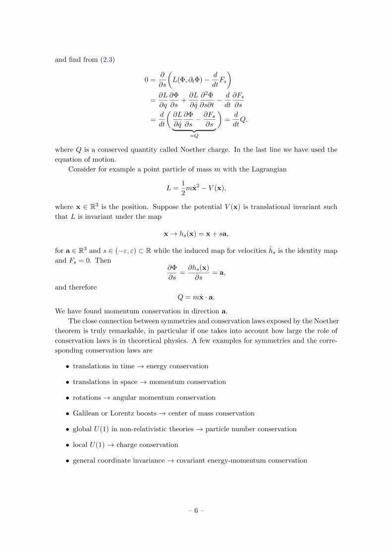
and find from (2.3)
0 =∂
∂s
(L(Φ, ∂tΦ)− d
dtFs
)=∂L
∂q
∂Φ
∂s+∂L
∂q
∂2Φ
∂s∂t− d
dt
∂Fs∂s
=d
dt
(∂L
∂q
∂Φ
∂s− ∂Fs
∂s︸ ︷︷ ︸=Q
)=
d
dtQ,
where Q is a conserved quantity called Noether charge. In the last line we have used the
equation of motion.
Consider for example a point particle of mass m with the Lagrangian
L =1
2mx2 − V (x),
where x ∈ R3 is the position. Suppose the potential V (x) is translational invariant such
that L is invariant under the map
x→ hs(x) = x + sa,
for a ∈ R3 and s ∈ (−ε, ε) ⊂ R while the induced map for velocities hs is the identity map
and Fs = 0. Then∂Φ
∂s=∂hs(x)
∂s= a,
and therefore
Q = mx · a.
We have found momentum conservation in direction a.
The close connection between symmetries and conservation laws exposed by the Noether
theorem is truly remarkable, in particular if one takes into account how large the role of
conservation laws is in theoretical physics. A few examples for symmetries and the corre-
sponding conservation laws are
• translations in time → energy conservation
• translations in space → momentum conservation
• rotations → angular momentum conservation
• Galilean or Lorentz boosts → center of mass conservation
• global U(1) in non-relativistic theories → particle number conservation
• local U(1) → charge conservation
• general coordinate invariance → covariant energy-momentum conservation
– 6 –

2.2 Classical mechanics in Hamiltonian description
In the Hamiltonian formulation of classical mechanics the physical information of a system
in encoded in the Hamiltonian H which is a function of position q, momenta p and time t.
The equations of motion are
dp
dt= −∂H
∂q,
dq
dt=∂H
∂p.
For systems which can also be described in the Lagrangian framework, the Hamiltonian is
given by the Legendre transformation
H(q, p, t) = pq − L(q, q, t),
where q is defined implicitly by
p =∂L
∂q.
The fundamental tool in Hamiltonian mechanics is the Poisson bracket. It is a map from
the space of pairs of differentiable functions of dynamical variables q and p to a single
differential function. For two such functions f, g we define a new function by
·, · :(f(q, p), g(q, p)
)→ f, g(q, p),
where
f, g =∂f
∂p
∂g
∂q− ∂f
∂q
∂g
∂p.
The Poisson bracket has three properties [Exercise: Show these.]
i) Bilinearity: λf + µg, h = λf, h+ µg, h,
i) Antisymmetry: f, g = −g, f,
iii) Jacobi identity: f, g, h+ g, h, f+ h, f, g = 0,
for differentiable functions f, g, h and for λ, µ ∈ R. By these properties the Poisson bracket
turns the space of functions of q and p into a Lie algebra. We will discuss much more about
Lie algebras later on.
If H does not explicitly depend on time, and for any differentiable function f(q(t), p(t))
which is evaluated on a trajectory that is a solution to the equations of motion, the time
derivative can be writtend
dtf(q(t), p(t)) = H, f.
One can formally solve this through an operator exp [∆tH, ·] for time translation,
f(q(t+ ∆t), p(t+ ∆t)) = exp [∆tH, ·] f(q(t), p(t)).
One says that H generates time translations in this sense. [Exercise: Work this out for an
infinitesimally small ∆t so that only linear terms need to be kept.]
– 7 –

Consider now again some map (q(t), p(t))→ (qs(t), ps(t)) with a continuous parameter
s and assume that this transformation is generated by Q in the sense that
d
dsqs(t) = Q, qs(t),
d
dsps(t) = Q, ps(t),
so that similar as for time translations one has for translations in s
f(qs+∆s(t), ps+∆s(t)) = exp [∆sQ, ·] f(qs(t), ps(t).
This transformation connects different solutions to the equations of motion if the operators
for translations in t and s commute,
exp [∆sQ, ·] exp [∆tH, ·] = exp [∆tH, ·] exp [∆sQ, ·] .
As we will show later in general terms, this is the case if
H,Q = 0.
But this actually means that Q is conserved, dQ/dt = 0.
We note here that the connection between symmetries and conservation laws is a little
less direct in the Hamiltonian formalism than in the Lagrangian one, but in any case the
connection is close.
2.3 Quantum mechanics
Starting from the Hamiltonian description it is most convenient to work in the Heisenberg
picture of quantum mechanics. Canonical quantisation maps the Poisson bracket of dif-
ferentiable functions in q and p to the commutator of the associated operators q and p in
some suitable Hilbert space H,
·, · → i
~[·, ·].
Here i is the imaginary unit, ~ denotes Planck’s constant and the commutator is defined
by
[A,B] = AB −BA.
In particular one has
p, q = 1→ i
~[p, q] = 1,
which is Heisenbergs commutation relation. The commutator equips H with a Lie alge-
bra in the same way the Poisson bracket does in the Hamiltonian description of classical
mechanics. In particular we have the properties
i) Bilinearity: [λA+ µB,C] = λ[A,C] + µ[B,C],
ii) Antisymmetry: [A,B] = −[B,A],
iii) Jacobi identity: [A, [B,C]] + [B, [C,A]] + [C, [A,B]] = 0,
– 8 –

for operators A,B,C and λ, µ ∈ R. Analogous to before the time dependance of the
operators is now described byd
dtA(t) =
i
~[H,A].
Observables which describe conservations laws are characterised by
[H,Q] = 0.
By the Jacobi identity, the space of all conserved quantities forms a closed Lie subalgebra.
As an example we consider angular momentum conservation of the electron in the
quantised hydrogen atom. Let the eigenstates of the Hamiltonian H be labelled by the
principal quantum number n, total angular momentum l and the quantum number for
the projection on the z-axis, m. Because angular momentum is conserved, the operator
commutes with the Hamiltonian,
[Lz, H] = 0,
and therefore for two eigenstates |n′, l′,m′〉, |n, l,m〉,
0 = 〈n′, l′,m′|[Lz, H]|n, l,m〉 = (m′ −m) 〈n′, l′,m′|H|n, l,m〉 .
Accordingly,
〈n′, l′,m′|H|n, l,m〉
can only be non-zero for m = m′, which is a selection rule.
One may also start from a conserved operator and construct the corresponding sym-
metry transformation. For a self-adjoint operator A ∈ H with
[H,A] = 0,
we define the unitary operator
UA(s) = eisA =
∞∑n=0
(isA)n
n!,
for s ∈ R. They obey the multiplication law
UA(s1) · UA(s2) = UA(s1 + s2),
for s1, s2 ∈ R and form a unitary one-parameter group. As an example consider the
momentum operator in position space defined as
p =~i
d
dx,
which generates infinitesimal translations. For a ∈ R the operator
exp(ia
~p)
= eaddx
generates finite translations, e. g.
eaddx f(x) = f(x+ a),
for a suitable function f .
– 9 –

3 Finite groups
Now that we discussed the close relation between symmetries and the mathematical concept
of a group it seems natural to start our analysis with simple cases, i.e. finite groups of low
order. The order ord(G) of a group G is defined to be the number of group elements.
3.1 Order 1
There is only one trivial group with a single element, namle e.
3.2 Order 2
The simplest symmetry transformation is a reflection,
P : x→ −x, (3.1)
which applied twice is the identity, i. e. PP = e. The parity transformation (3.1) has the
simplest finite group structure involving only two elements. The group is known as the
cyclic group Z2 with the following multiplication table.
Z2 e P
e e P
P P e
The group Z2 has many manifestations for example in terms of reflections about the sym-
metry axis of an isosceles triangle.
Studying higher order groups will naturally involve more elements which can manifest in
more symmetries, e.g. the equilateral triangle is symmetric under reflections about any of
its three medians as well as rotations of 2π3 around its center,
which is described by a group of order six. In general we denote the elements of a group
of order n by e, a1, a2, ..., an−1 where e denotes the identity element.
– 10 –

3.3 Order 3
There is only one group of order three which is Z3 with the following multiplication table.
Z3 e a1 a2
e e · e = e e · a1 = a1 e · a2 = a2
a1 a1 · e = a1 a1 · a1 = a2 a1 · a2 = e
a2 a2 · e = a2 a2 · a1 = e a2 · a2 = a1
Sometimes one writes this compactly as follows.
Z3 e a1 a2
e e a1 a2
a1 a1 a2 e
a2 a2 e a1
The group elements can be written as e, a1 = a, a2 = a2, with the law that a3 = e. One
says that a is an order three element. The structure of the group is completely fixed by
the multiplication table. However, this gets rather cumbersome, in particular for larger
groups and it is convenient to use another characterisation of the group elements and their
multiplication laws, the so-called presentation. For example Z3 has a presentation
〈a | a3 = e〉 .
The first part of the presentation lists the group elements from which all others can be
constructed – the so-called generators – while the second part gives the rules needed to
construct the multiplication table.
This generalises to the cyclic group Zn of order n ∈ N which has the group elements
e, a, a2, ..., an−1 and a presentation is given by
〈a | an = e〉 . (3.2)
One distinguishes between a group G which is an abstract entity defined by the set of
its group elements and their multiplication table (or, equivalently, a presentation) and a
representation of a group.
Representation. A representation can be seen as a manifestation of the group multipli-
cation laws in a concrete system or, in other words, a kind of incarnation of the group. For
example, the group Z3 has a representation in terms of rotations by 2π3 around the center
of an equilateral triangle. Zn has also a representation
1, ei2πn , e2i 2π
n , ..., e(n−1)i 2πn , (3.3)
where the group elements are represented equidistantly on the unit circle in the complex
plane and the action of the generator a is represented by a rotation of 2πn around the centre.
– 11 –

.
....
.
.
.. . .
.
C
Often one works with representations as operations in a vector space.
A matrix representation R of a group G on a vector space V is a group homomorphism
R : G→ GL(V )
onto the general linear group GL(V ) on V , i.e. a map from a group element g to a matrix
R(g) such that
R(g1 · g2) = R(g1) · R(g2)
for all g1, g2 ∈ G. We define the dimension of the representation R by
dim(R) = dim(V )
and denote the identity element of a group by e and of a representation by 1.
3.4 Order 4
At order four there are two different groups. Again there is Z4 which in the representations
(3.3) reads 1, i,−1,−i. The other group is the dihedral group D2 with the multiplication
table
D2 e a1 a2 a3
e e a1 a2 a3
a1 a1 e a3 a2
a2 a2 a3 e a1
a3 a3 a2 a1 e
The fact that the multiplication table is symmetric shows that D2 is abelian, ai ·aj = aj ·ai.Two representations of D2 are(
1 0
0 1
),
(1 0
0 −1
),
(−1 0
0 1
),
(−1 0
0 −1
),
and f1(x) = x, f2(x) = −x, f3(x) =
1
x, f4(x) = −1
x
.
For both groups of order four we can form a subgroup, namely Z2. It is straight forward
to see from the presentation (3.2) for Z4,
〈a | a4 = e〉 ,
– 12 –

that the group generated by a2 is Z2. The same goes for the group generated by ai ∈ D2
for any choice i ∈ 1, 2, 3. For D2 one can actually go on and write it as a direct product
of two factors Z2,
D2 = Z2 ⊗ Z2.
We use here the notion of a direct product.
Direct product. Let (G, ) and (K, ∗) be two groups with elements ga ∈ G, a ∈1, ..., nG and ki ∈ K, i ∈ 1, ..., nK respectively. The direct product is a group (G⊗K, ?)of order nGnK with elements (ga, ki) and the multiplication rule
(ga, ki) ? (gb, kj) = (ga gb, ki ∗ kj).
Since and ∗ act on different sets, they can be taken to be commuting subgroups and we
simply write gaki = kiga for the elements of G⊗K.
As long as it is clear we denote for notational simplicity the group (G, ) by G and the
group operation as g1 g2 = g1g2. [Exercise: Show that D2 = Z2 ⊗ Z2 but Z4 6= Z2 ⊗ Z2.]
3.5 Lagrange’s theorem
If a group G of order N has a subgroup H of order n, then N is necessarily an integer
multiple of n.
Consider a group G = ga | a ∈ 1, ..., N with subgroup H = hi | i ∈ 1, ..., n ⊂G. Take a group element ga ∈ G but not in the subgroup, ga /∈ H. Then it follows that
also gahi is not in H, gahi /∈ H, because if there would exist hj ∈ H such that gahi = hjthen ga = hjh
−1i ∈ H which would object our assumption. Continuing in this way we can
construct the disjoint cosets
gaH = gahi | i ∈ 1, ..., n
and write G as a (right) coset decomposition
G = H ∪ g1H ∪ ... ∪ gkH,
with k ∈ N. Therefore the order of G can only be a multiple of its subgroup’s order,
N = nk.
As an immediate consequence, groups of prime order cannot have subgroups of smaller
order. Hence for a group of prime order p all elements are of order one or order p and thus
G = Zp.
3.6 Order 5
By Lagrange’s theorem there is only Z5.
– 13 –

3.7 Order 6
We now know that there are at least two groups of order six: Z6 and Z2 ⊗ Z3 but the
question is whether they actually differ. Let us consider Z2⊗Z3. The generator a of Z3 is
an order-three element, by which we mean a3 = e. In contrast, the generator b of Z2 is an
order-two element and thus a3 = e = b2 and we also have ab = ba. Now (ab)6 = a6b6 = e
and ab is in fact an order-six element in Z2 ⊗ Z3 and one can infer
Z6 = Z2 ⊗ Z3.
To construct another order six group we again take an order-three element a and an
order-two element b. The set
e, a, a2, b, ab, a2b,
together with the relation ba = a2b 6= ab forms the dihedral group D3 which is non-abelian.
A presentation is given by
〈a, b | a3 = e, b2 = e, bab−1 = a−1〉 .
D3 is the symmetry group of the equilateral triangle
A
C
B
where a is a rotation by 2π3 (ABC → BCA) and b is a reflection (ABC → BAC). Higher
dihedral groups have higher polygon symmetries.
D4 D5
The group can also be represented by permutations as indicated above. The element a
corresponds to a three-cycle A→ B → C → A(A B C
B C A
)(3.4)
whereas the element b is a two-cycle: A→ B → A(A B
B A
). (3.5)
In general the n! permutations of n objects form the symmetric group Sn. From (3.4) and
(3.5) we see
D3 = S3.
– 14 –

The group operation for a k-cycle can be represented by k × k matrices, e.g. a three-cycle
can be represented by (3× 3) matrices0 1 0
0 0 1
1 0 0
ABC
=
BCA
.
3.8 Order 8
From what we know already we can immediately write down four order eight groups which
are not isomorphic to each other since they contain elements of different order: Z8, Z2 ⊗Z2 ⊗ Z2, Z4 ⊗ Z2. Additionally there is the dihedral group D4 and a new group Q called
the quaternion group.
Let us directly focus on the latter. An element q of the deduced quaternion vector
space H generalises the complex numbers,
q = x0 + x1i + x2j + x3k,
q = x0 − x1i− x2j− x3k,
with xi ∈ R and the relation
i2 = j2 = k2 = −1,
for the imaginary units as well as
ij = −ji = k,
and cyclic permutations thereof. For q ∈ H
N(q) =√qq,
defines a norm with
N(qq′) = N(q)N(q′).
A finite group of order eight can now be taken to be the set
1, i, j,k,−1,−i,−j,−k,
and is called the quaternion group Q. [Exercise: Convince yourself that Q is a closed group,
indeed.]
A matrix representation of the quaternion group Q is given by the Pauli matrices
1, i, j,k,−1,−i,−j,−k = 1,−iσ1,−iσ2,−iσ3,−1, iσ1, iσ2, iσ3
with the property
σjσk = δjk + iεjklσl,
and the concrete expressions
σ1 =
(0 1
1 0
), σ2 =
(0 −ii 0
), σ3 =
(1 0
0 −1
).
– 15 –

3.9 Permutations
The permutations of n objects can be represented by the symbol(1 2 3 ... n
a1 a2 a3 ... an
)
and all possible such permutations form a group (of order n!), the symmetric group Sn.
Every permutation can uniquely be resolved into cycles, e.g.(1 2 3 4
2 3 4 1
)∼ (1234),(
1 2 3 4
2 1 3 4
)∼ (12)(3)(4),(
1 2 3 4
3 1 2 4
)∼ (132)(4).
Any permutation can also be decomposed into a product of two-cycles,
(a1a2a3...an) ∼ (a1a2)(a1a3)...(a1an).
The symmetric group Sn has a subgroup of even permutations An ⊂ Sn of order n!/2.
Notice that the odd permutations do not form a subgroup since there is no unit element.
3.10 Cayley’s theorem
Every group of finite order n is isomorphic to a subgroup of Sn.
Let G = ga | a ∈ 1, ..., n be a group and associate the group elements with the
permutations
ga → Pa =
(g1 g2 ... gng1ga g2ga ... gnga
).
This construction leaves the multiplication table invariant,
gagb = gc → PaPb = Pc,
and Pa | a ∈ 1, ..., n is called the regular representation of G and it is by construction
a subgroup of Sn.
3.11 Some notations and concepts
Conjugate with respect to a group element. For a group G = ga | a ∈ 1, ..., nwe define the conjugate to an element ga ∈ G with respect to the element g ∈ G as
ga = g ga g−1.
With this definition, multiplication rules remain unmodified under conjugation,
gagb = gc → gagb = gc
– 16 –

since
gga g−1g︸︷︷︸e
gbg−1 = ggagbg
−1 = ggcg−1.
Note that if we have [g, ga] = 0, then the conjugate of ga with respect to g is just ga again.
Equivalence classes of group elements. For a group G and an element ga we define
the equivalence class Ca to consist of all ga that are conjugate to ga with respect to some
element g,
Ca = ga = g ga g−1 | g ∈ G.
Now take another group element gb ∈ G but such that gb /∈ Ca. The set of all conjugates
forms the class Cb,
Cb = gb = g gb g−1 | g ∈ G,
and so we can go on. Note that the classes are disjoint, i. e. there can be no group elements
that are simultaneously in two classes. [Exercise: Show this!] In this way we can decompose
G into a set of equivalence classes
G = C1 ∪ C2 ∪ ... ∪ Ck.
Note that the unit element e is always forming an equivalence class of it’s own and tra-
ditionally it is denoted by C1. Also, if the group is abelian, each group element forms its
own equivalence class so the concepts is only really interesting for non-abelian groups.
Normal or invariant subgroup. Let G be a group and H ⊂ G a subgroup. Assume
now that for all elements of the subgroup hi ∈ H the conjugates with respect to any group
element g ∈ G stay in H, that is
g hi g−1 ∈ H.
In this case H is called an invariant or normal subgroup. One can also formulate this by
saying that for for a normal subgroup, all the equivalence classes of its elements must be
entirely part of the subgroup. Normal subgroups are rather special subgroups and one uses
the notation H / G as a stronger version of H ⊂ G.
As a first example, consider a direct product group G = H1 ⊗ H2. In that case H1
and H2 are invariant or normal subgroups of G. As a second example consider Z4 =
1,−1, i,−i. It has the invariant subgroup Z2 = 1,−1, for example i1,−1(−i) =
1,−1. As a third example, consider the quaternion group
Q = 1, i, j,k,−1,−i,−j,−k,
which has an invariant subgroup Z4 = 1,−1, i,−i, for example j1,−1, i,−ij−1 =
1,−1,−i, i.
– 17 –

Quotient group. Let us consider a map from a group G to a smaller group K,
G→ K,
ga → ka,
such that gagb = gc → kakb = kc. Now we take H to be the kernel of this map, i. e. the set
of all group elements of G that are mapped to the unit element of K,
H = ga ∈ G | ga → e ⊂ G.
The so-constructed H is then a normal subgroup because for all hi ∈ H
ghig−1 → kek−1 = e.
Now let us go the other way. Let us assume that G has a normal subgroup H. We will
now use H to build sets of group elements and to define a multiplication between these
sets. More specific, consider the set
gH = g h | h ∈ H.
This is known as a left coset. Now take two cosets gaH and gbH and let H = eH be
the trivial coset. We define the multiplication of cosets through the multiplication of their
elements,
(gahi)︸ ︷︷ ︸∈gaH
(gbhj)︸ ︷︷ ︸∈gbH
= gagb g−1b higb︸ ︷︷ ︸hi
hj = gagb hihj︸︷︷︸∈H
∈ gagbH.
Note that we have assumed that H is a normal subgroup. This shows that the cosets can
be multiplied,
(gaH)(gbH) = (gagbH),
in the same way as the original group elements ga and gb.
In other words, the set of cosets gaH has a group structure itself where the identity
element is simply the trivial coset H. This group is called the quotient group G/H. The
quotient group is a homomorphic image of the original group G, but it is in general not a
subgroup.
As an example consider the quaternionic group Q = 1, i, j,k,−1,−i,−j,−k which,
as we have shown before, has a normal or invariant subgroup Z4 = 1,−1, i,−i. The
latter is the also the unit element of the quotient group Q/Z4, which is of order 8/4 = 2.
Its other element besides the unit element is jZ4 = j1,−1, i,−i = j,−j,−k,k. One
sees easily that (jZ4)(jZ4) = Z4 so that Q/Z4 = Z2 as expected.
To summarize, if G contains a non-trivial normal subgroup H, we can construct a
smaller group, the quotient group G/H, essentially by “dividing out” H. For example
starting from a direct product group H1⊗H2 and “dividing out” H2 leads to H1⊗H2/H2 =
H1.
However, not all groups have normal subgroups. For example, one can show that the
quotient group G/H has no normal subgroup if H is the maximal normal subgroup.
– 18 –

Simple group. A simple group is a group without (non-trivial) normal subgroups. The
simple groups are particularly interesting for mathematicians because they are elementary
in the sense that other groups can be reduced to them.
Relatively recently (in 2004), all finite simple groups have been classified with the
result that and there are
• the cyclic groups Zp for p prime
• the alternating groups An with n ≥ 5
• 16 infinite families of groups of Lie type (not to be confused with continuous Lie
groups)
• 26 sporadic groups
However, a detailed discussion of this classification goes beyond the scope of these lectures.
3.12 Representations
Let V be a N dimensional vector space with an orthonormal basis |i〉,
N∑i=1
|i〉 〈i| = 1, 〈i|j〉 = δij ,
where 1 is the identity element in the space of N -dimensional matrices GL(V ). Let G be a
group of order n with representation R on V such that the action of g ∈ G is represented
by
|i〉 → |i(g)〉 = Mij(g) |j〉 ,
where M(g) ∈ GL(V ). Then for ga, gb, gc, g ∈ G and gagb = gc,
M(ga) ·M(gb) = M(gc),
M(g−1)ij = (M(g)−1)ij .
The representation is called trivial if M(g) = 1 for all g ∈ G. The representation R is
called reducible if one can arrange M(g) in the form
M(g) =
(M [1](g) 0
N(g) M [⊥](g)
),
where M [1](g) ∈ GL(V1) acts on the subspace V1 ⊂ V of dimension d1, M [⊥](g) ∈ GL(V ⊥1 )
on its orthogonal complement V ⊥1 ⊂ V of dimension N − d1 and N(g) is a (N − d1) × d1
matrix. Then for g, g′ ∈ G
M [1](gg′) = M [1](g) ·M [1](g′),
M [⊥](gg′) = M [⊥](g) ·M [⊥](g′),
as well as
N(gg′) = N(g) ·M [1](g′) +M [⊥](g) ·N(g′).
– 19 –

One can in fact simplify this further. With
W =1
ord(G)
∑g∈G
M [⊥](g−1) ·N(g),
we diagonalise the representation(1 0
W 1
)·
(M [1] 0
N M [⊥]
)·
(1 0
−W 1
)=
(M [1] 0
0 M [⊥]
),
using
W ·M [1](g1) =1
ord(G)
∑g∈G
M [⊥](g−1) ·N(g) ·M [1](g1)
= −N(g1) +1
ord(G)
∑g′∈G
M [⊥](g1g′−1) ·N(g′)
= −N(g1) +M [⊥](g1) ·W,
with g′ = gg1. In this basis we say R is completely reducible,
R = R1 ⊕R⊥1 .
If R⊥1 is reducible we can further reduce until there are no subspaces left,
R = R1 ⊕R2 ⊕ ...⊕Rk,
with k ∈ N.
3.13 Schur’s lemmas
From the notation established before we write the action of a g ∈ G in the subspace V1 ⊂ Vas
|a〉 → |a(g)〉 = M[1]ab (g) |b〉 ,
where |a〉 is a orthonormal basis of V1. Since V1 is a subspace of V we can write
|a〉 = Sai |i〉 ,
with S a d1 ×N matrix. Now we write the group action
|a〉 → |a(g)〉 = M[1]ab (g) |b〉 = M
[1]ab (g) Sbi |i〉 ,
or equivalently
|a〉 = Sai |i〉 → Sai |i(g)〉 = Sai Mij(g) |j〉 .
Therefore,
R reducible ⇒ Sai Mij(g) = M[1]ab (g) Sbj for all g ∈ G. (3.6)
– 20 –

Schur’s first lemma: If matrices of two irreducible representations of different dimen-
sion can be related as in (3.6), then S = 0.
If now d1 = N , S is an N × N matrix and if |a〉 and |j〉 span the same space the
representations R and R1 are related by a similarity transformation
M [1] = S ·M · S−1.
Thus for S 6= 0 we conclude that either R is reducible or there is a similarity relation.
Schur’s second lemma: Let R be an irreducible representation. Any matrix S with
M(g) · S = S ·M(g)
for all g ∈ G is proportional to 1.
If |i〉 is an eigenket of S then |i(g)〉 is also an eigenket,
M(g)S |i〉︸︷︷︸λ|i〉︸ ︷︷ ︸
λ|i(g)〉
= SM(g) |i〉︸ ︷︷ ︸|i(g)〉
⇒ S = λ1.
Let Ra,Rb be two irreducible representations of dimension da and db respectively.
Construct the map
S =∑g∈G
M [a](g) ·N ·M [b](g−1),
where N is any da × db matrix. Then for g ∈ G
M [a](g) · S = S ·M [b](g).
For Ra 6= Rb by Schur’s first lemma
1
ord(G)
∑g∈G
M[a]ij (g) M [b]
pq (g−1) = 0.
On the other hand for Ra = Rb by Schur’s second lemma
1
ord(G)
∑g∈G
M[a]ij (g) M [a]
pq (g−1) =1
daδiqδjp.
Combining these two results leaves us with
1
ord(G)
∑g∈G
M[a]ij (g) M [b]
pq (g−1) =1
daδiqδjpδ
ab.
Let us define the scalar product
(i, j) =1
ord(G)
∑g∈G〈i(g)|j(g)〉 , (3.7)
– 21 –

where |j(g)〉 = M(g) |j〉. It is invariant under the group action
(i(ga), j(ga)) =1
ord(G)
∑g∈G〈i(gag)|j(gag)〉
=1
ord(G)
∑g′∈G〈i(g′)|j(g′)〉
= (i, j),
where g′ = gag runs over all group elements. Therefore for v,u ∈ V
(M(g−1)v,u) = (v,M(g)u).
On the other hand
(M †(g)v,u) = (v,M(g)u),
where M † is the Hermitian conjugate of M and therefore
M †(g) = M(g−1) = M−1(g).
Therefore all representations of finite groups are unitary with respect to the scalar prod-
uct (·, ·) that we have constructed as an average over the group elements in (3.7).
[Exercise: Use the scalar product (·, ·) to show that every reducible representation is
necessarily also completely reducible, which means that it can be brought to block diagonal
form. Hint: use that there is an invariant sub-vector-space and consider the orthogonal
complement.]
3.14 Crystals
Crystals live in between finite and infinite groups; they have symmetries of both kinds.
A crystal in three dimensions is defined as a lattice which is invariant under discrete
translations of the form
T = n1u1 + n2u2 + n3u3, (3.8)
with three linearly independent ui ∈ R3 and ni ∈ Z. The entire symmetry group of a
crystal (the so-called space group) contains besides translations also rotations, reflections,
and combinations thereof. A subgroup that consists of rotations and reflections (and their
combinations of course) that leave one point invariant, is know as the smaller point group.
We will not go into further detail here but mention that in three dimensions there are 230
crystallographic space groups and 32 crystallographic point groups. The latter determine
macroscopic properties of crystals. Point groups are also used to classify molecules, but
because they do not need to have translational symmetries, there are more point groups.
A crystal in two dimensions may also be called an ornament and the corresponding
symmetry group is sometimes called a wallpaper group. In two dimensions there are 17
space groups and only 9 crystallographic point groups: the cyclic groups Z2, Z3, Z4 and Z6
as well as the dihedral groups D2, D3, D4 and D6. In addition to this there is the trivial
group Z1 = D1 with only one element. It is remarkable that there are no 5-fold, 7-fold or
higher n-fold rotation symmetries possible. This is subject to the following theorem.
– 22 –

Crystallographic restriction theorem: Consider a crystal invariant under rotations
through 2π/n around an axis. Then n is restricted to n ∈ 1, 2, 3, 4, 6.
z
T1
T2
T3
T4
t21
First, the case n = 1 is trivial and we can exclude it and concentrate on the other cases.
Consider a translation vector T1. By rotations it gets transformed to T2,T3, ...,Tn . By
the group property of the space group, also the differences tij = Ti − Tj are translation
vectors and by construction they are orthogonal to the rotations axis, which we may take
to coincide with the z-axis. Take now the minimum of the differences,
|t| = mini,j
(|tij |),
and without loss of generality normalise |t| = 1. Take now a point A on the rotational
symmetry axis which by t gets translated to another symmetry point B. Rotation by
an angle ϕ around A brings B to B′. Similar, rotation by ϕ around B brings A to A′.
Because A′ and B′ are also symmetry points, the difference A′B′ must be a translation
vector parallel to AB, and so we can infer that A′B′ = p ∈ N0.
A B
ϕ
|t|
A′B′
• •
••
With
A′B′ = 1 + 2 sin(ϕ− π
2
)= 1− 2 cos(ϕ),
we conclude
cos(ϕ) =1− p
2,
– 23 –

and thus the possible values are
p ∈ 0, 1, 2, 3,
⇒ ϕ ∈π
3,π
2,2π
3, π,
⇒ n ∈ 6, 4, 3, 2.
This closes the proof of the restriction theorem above.
Quasicrystals may have elements or subregions with five-fold or other symmetries but
have in fact no periodic structure (3.8), for example a Penrose tiling.
– 24 –

4 Lie groups and Lie algebras
Lie groups can be defined as differentiable manifolds with a group structure. In contrast to
the finite groups we have discussed before they have now an infinite number of elements.
Let us start with a few examples.
4.1 Examples for Lie groups
• G = R, the additive group of real numbers. The group “product” is here the addition,
the inverse of an element is its negative and the neutral or unit element is zero. This
is clearly an abelian group.
• G = R∗+, the multiplicative group of positive real numbers. Also an abelian group.
• G = GL(n,R), the general linear group of real n × n matrices g with det(g) 6= 0
(such that they are invertible). Similarly, G = GL(n,C), the general linear group of
complex n× n matrices. These groups are non-abelian for n > 1.
• G = SL(n,R) the special linear group is a subgroup of GL(n,R) with det(g) = 1.
This is a more general notion, the S for special usually means det(g) = 1.
• G = O(n), the orthogonal group of real n×n matrices R with RTR = 1. This imme-
diately implies det(R) = ±1. Again this is a subgroup of GL(n,R). As a manifold,
O(n) is not connected. One component is the subgroup SO(n) with det(R) = 1,
the other is a separate submanifold where det(R) = −1. One can understand O(n)
as the group of rotations and reflections in the n-dimensional Euclidean space. The
simplest non-trivial case is for n = 2 where SO(2) consists of elements of the form
R(θ) =
(cos(θ) − sin(θ)
sin(θ) cos(θ)
).
This is clearly isomorphic to the group U(1) of complex phases eiθ. SO(n) is non-
abelian for n > 2.
• G = U(n), the unitary group of complex n × n matrices U with U †U = 1. Now we
immediately infer that det(U) is a complex number with absolute value 1. U(n) is
non-abelian for n > 1.
• G = SU(n), the special unitary group with unit determinant. Plays an important
role in physics and we will discuss in particular SU(2) and SU(3) in more detail.
• G = O(r, n − r) the indefinite orthogonal group of n × n matrices R that leaves
the metric η = diag(−1, . . . ,−1,+1, . . . ,+1) with r entries −1 and n− r entries +1
invariant, in the sense that RT ηR = η. An example is O(1, 3), the group of Lorentz
transformations in d = 1 + 3 dimensions.
– 25 –

• G = Sp(2n,R) is the symplectic group of 2n×2n matrices M that leaves a symplectic
bilinear form
Ω =
(0 +1n−1n 0
)(4.1)
invariant in the sense that MTΩM = Ω. Here 1n is the n dimensional unit matrix
and similarly 0. This is obviously a subgroup of GL(2n,R). There is also a complex
version Sp(2n,C).
[Exercise: Convince yourself that all these examples are groups and also differentiable
manifolds.]
Lie groups have very nice features and a rich mathematical structure because they are
both, groups and manifolds. We will now first introduce Lie groups and Lie algebras from
an algebraic point of view, and subsequently also briefly introduce a differential-geometric
characterization.
4.2 Algebraic approach to Lie groups and Lie algebras
Because a Lie group is also a manifold, group elements can be labeled by a (usually multi-
dimensional) parameter or coordinate ξ = (ξ1, . . . , ξm), i.e. we can write them as g(ξ).
Without loss of generality we can assume that ξ = 0 corresponds to the unit element,
g(0) = 1. Let us now consider infinitesimal transformations. We can write them as
g(dξ) = 1+ idξjTj + . . . , (4.2)
where we use Einsteins summation convention and the ellipses stand for terms of quadratic
and higher order in dξ. Note that we can write
iTj =∂
∂ξjg(ξ)
∣∣∣ξ=0
. (4.3)
Formally, the objects iTj constitute a basis of the tangent space of the Lie group manifold
at the position of the unit element g(ξ) = 1, which is at ξ = 0. The factor i is conventional
and used by physicists, while mathematicians usually work in a convention without it. The
Tj are also known as the generators of the Lie algebra, to which we turn in a moment. The
generators constitute a basis such that any element of the Lie algebra can be written as a
linear superposition vjTj .
A very important idea is now that one can compose finite group elements, at least in
some region around the unit element, out of very many infinitesimal transformations. In
other words one writes
g(ξ) = limN→∞
(1+
iξjTjN
)N= exp
(iξjTj
). (4.4)
One recognizes here that the limit in (4.4) would give the exponential if Tj were just
numbers, and one can essentially use this limit to define also the exponential of Lie algebra
elements. Alternatively, the exponential may also be evaluated as the usual power series
exp(iξjTj
)= 1+ iξjTj +
1
2
(iξjTj
)2+
1
3!
(iξjTj
)3+ . . .
– 26 –

Note that for α, β ∈ R one can combine
exp(iαξjTj
)exp
(iβξjTj
)= exp
(i(α+ β)ξjTj
). (4.5)
Such transformations (for fixed ξ) form a one-parameter subgroup. [Exercise: Verify this.]
However, it is more difficult to combine transformations exp(iξjTj
)and exp
(iζjTj
)when ξ is not parallel to ζ. The reason is that ξjTj and ζjTj can not be assumed to com-
mute. To combine two transformations, one needs to use the Baker-Campbell-Hausdorff
formula
exp(X) exp(Y ) = exp(Z(X,Y )), (4.6)
with
Z(X,Y ) = X + Y +1
2[X,Y ] +
1
12[X, [X,Y ]]− 1
12[Y, [X,Y ]] + . . . (4.7)
This shows that it is crucial to know how to calculate commutators between the Lie algebra
elements.
For transformations close to the identity element we can write using (4.6) and (4.7)
exp(iξjTj
)exp
(iζjTj
)= exp
(iωjTj
), (4.8)
with
ωl = ξl + ζ l − 1
2ξjζkf l
jk + . . . ,
where the ellipses stand now for terms of quadratic and higher order in ξ and / or in ζ.
We are using here the structure constants f ljk of the Lie algebra defined through the
commutator
[Tj , Tk] = i f ljk Tl. (4.9)
The structure constants are obviously anti-symmetric,
f ljk = −f l
kj .
Equation (4.9) tells that the commutator of two generators can itself be expressed as a
linear combination of generators. Together with eqs. (4.6) and (4.7) this makes sure that
the group elements (4.4) can be multiplied and indeed form a group. In other words, if
eq. (4.9) holds, we can multiply group elements as in eq. (4.8) to yield another term of the
same structure such that they form a group. On the other side, one could also start from
the group multiplication law and demand that the left hand side of (4.8) can be written
as on the right hand side. At order ∼ ξζ this implies then a relation of the form (4.9).
But (4.9) also makes sure that linear combinations of generators, which obviously form
a vector space, constitute a Lie algebra. As usual, the Lie bracket [·, ·] has the properties
i) Bilinearity: [λA+ µB,C] = λ[A,C] + µ[B,C],
ii) Antisymmetry: [A,B] = −[B,A],
iii) Jacobi identity: [A, [B,C]] + [B, [C,A]] + [C, [A,B]] = 0.
– 27 –

From the Jacobi identity for the generators
[Tj , [Tk, Tl]] + [Tk, [Tl, Tj ]] + [Tl, [Tj , Tk]] = 0, (4.10)
one infers for the structure constants
f mjn f n
kl + f mkn f n
lj + f mln f n
jk = 0. (4.11)
For unitary Lie groups where g† = g−1 one has Tj = T †j and that in that case the
structure constants are real,
f ljk =
(f ljk
)∗.
[Exercise: Check that.]
Representations. The commutation relation (4.9) and in particular the structure con-
stants define a Lie algebra similar as the multiplication rules do for a group. Again one
distinguishes between a particular Lie algebra as an abstract entity and a concrete incar-
nation or representation of it.
A first example is the fundamental representation
(T(F )j )mn = (tj)
mn. (4.12)
For SU(N), the generators in the fundamental representation tj are hermitian and traceless
N ×N matrices, e.g. the three Pauli matrices for SU(2) and the eight Gell-Mann matrices
for SU(3).
From the Jacobi identity (4.11), one can see that the structure constants can actually
be used to construct another representation, the so-called adjoint representation. Here one
sets the matrices to
(T(A)j )mn = if m
jn . (4.13)
Indeed, one can check that this fulfills the commutation relation (4.9). [Exercise: Do it!]
The dimension of the adjoint representation equals the number of generators of the
Lie algebra. For example, the Lie algebra of SU(3) has 8 generators and accordingly the
adjoint representation is given by 8× 8 matrices.
The fundamental and the adjoint representation are the most important representa-
tions of a Lie algebra and we will need them often in the following. However, there are
many more and they all induce corresponding representations of the Lie group through the
exponential map (4.4).
One remark of caution should be made here: Group elements in some neighborhood
of the unit elements can be written in the exponential form (4.4). However, it is not at all
clear that all group elements can be written is this way. For a group where the manifold
has two disconnected components, such as O(N), this can only be the case for the part
that is connected to the identity element. Only for groups that are connected and compact
one can show that the exponential map (4.4) reaches indeed all elements.
– 28 –

4.3 Differential geometric approach to Lie groups and Lie algebras
Now that we understand already some of the properties of Lie groups and Lie algebras, let
us discuss them also from a geometric point of view. It is interesting to consider the group
multiplication as a map on the group manifold,
Lh : G→ G, Lh(g) = hg. (4.14)
This is the so-called left translation.
Recall that in (4.3) we have introduced the generators Tj as a basis for the tangent
space of the group manifold G at the identity g = 1 or ξ = 0.
More formally, one can construct the tangent space of a manifold as a basis for vectors,
which are in turn defined through curves. Let us review this construction. We first consider
a curve in the group manifold parametrized by some parameter α ∈ R and we assume that
it goes through the unit element g(α0) = 1. We can write the curve as g(α), or in terms
of coordinates ξ on the group manifold as ξ(α) such that g(α) = g(ξ(α)) and ξ(α0) = 0.
Now consider the derivative
d
dαg(α)
∣∣∣α=α0
=∂
∂ξjg(ξ)
∣∣∣ξ=0
dξj
dα= iTj
dξj
dα.
This is now an element of the tangent space T1(G) of the group manifold at the point
where g(ξ) = 1. Any element of this vector space can be written as a linear combination
of the basis elements
iTj =∂
∂ξjg(ξ)
∣∣∣ξ=0
.
Interestingly, this basis for T1(G) can be extended to a basis for the tangent spaces at
other positions of the group manifold. To that end we can use the left translation (4.14).
Specifically, from the curve g(α) we can construct another curve through the left transla-
tion (4.14)
g(α) = Lh(g(α)) = hg(α).
The derivative at the point α0 is now
d
dαg(α)
∣∣∣α=α0
=∂
∂ξjhg(ξ)
∣∣∣ξ=0
dξ
dα.
– 29 –

One observes that a basis for the tangent space Th(G) is given by
iTj(h) =∂
∂ξjhg(ξ)
∣∣∣ξ=0
= h∂
∂ξjg(ξ)
∣∣∣ξ=0
= i hTj . (4.15)
In this way we can actually get a basis for the tangent spaces everywhere in the entire
group manifold. It is quite non-trivial that the tangent spaces can be parametrized by a
single set of basis functions iTj(h). One says that the manifold G is parallelizable.
Formally, the map (4.15) between the tangent spaces T1(G) and Th(G) is an example
for a pushforward, induced by the map (4.14) on the manifold itself. One also writes this
as
Tj(h) = Lh∗Tj(e) = Lh∗Tj .
One may now construct vector fields on the entire manifold as linear combinations,
V (h) = vj(h)Tj(h). (4.16)
Such a vector field is called left invariant if
Lg∗V (h) = V (gh).
Because the basis Tj(h) is left-invariant by construction, the vector field (4.16) is left-
invariant when the coefficients vj(h) are independent of the position on the manifold, i. e.
independent of h. [Exercise: Check that Tj(h) is left-invariant.]
In summary, we may say that the generators of the Lie algebra Tj induce actually a left-
invariant basis for vector fields on the entire group manifolds. One may even understand
the Lie algebra itself as an algebra of left-invariant vector fields. The Lie bracket is then
introduced as the Lie derivative of vector fields.
4.4 Examples for matrix Lie algebras
Let us end this section with a few examples for Lie algebras corresponding to matrix Lie
groups introduced previously.
• su(n) is the Lie algebra corresponding to the group SU(n). We write the group
elements as U = exp(it). From U †U = 1 one infers t† = t. Writing this in com-
ponents, the real part is symmetric, Re(tnm) = Re(tmn), and the imaginary part is
anti-symmetric, Im(tnm) = −Im(tmn). Moreover, we have the condition det(U) = 1.
The latter can be rewritten as
det(U) = exp(ln(det(U))) = exp(Trln(U)) = exp(iTrt) = 1, (4.17)
so that we need Trt = 0. These arguments show that the Lie algebra su(n) as a
real vector space has n2 − 1 linearly independent generators Tj .
• so(n) is the Lie algebra corresponding to the group SO(n). Here we write the group
elements as R = exp(it) and they are real matrices such that RTR = 1. For the Lie
algebra elements we have again t = t†. In order for an infinitesimal transformation
R = 1+it to be real, the components tmn must be imaginary, and therefore also anti-
symmetric. The condition Trt = 0 is then automatically fulfilled. These arguments
show that the Lie algebra so(n) has n(n− 1)/2 linearly independent generators Tj .
– 30 –

• sp(2n) is the Lie algebra corresponding to the group Sp(2n). The group elements
R = exp(it) are real matrices that satisfy RTΩR = Ω with Ω = −ΩT given in (4.1).
For an infinitesimal transformation R = 1+ it one finds the condition
Ωt+ tTΩ = Ωt− tTΩT = Ωt− (Ωt)T = 0. (4.18)
In other words, Ωt must be symmetric. These arguments show that the Lie algebra
sp(2n) has n(2n+ 1) linearly independent generators Tj .
[Exercise: Consider the three dimensional rotation group SO(3). Find convenient gener-
ators Tj of the Lie algebra so(3) such that TrTjTk = 2δjk, and work out the structure
constants f ljk . For rotations around a particular axis (e.g. the z-axis), work out the
exponential map explicitly. Show also that SO(3) is non-abelian.
Consider also the Lie algebra su(2), find convenient generators normalized now such
that TrTjTk = 12δjk, and show that the structure constants are the same as for so(3). In
this sense the two Lie algebras actually agree, su(2) = so(3), even though the Lie groups
SU(2) and SO(3) differ.]
– 31 –

5 SU(2)
5.1 The Lie algebra and its representations
The Lie algebra su(2) of SU(2) is one of the smallest non-trivial Lie algebras. It plays an
important role in physics not only because it is isomorphic to the Lie algebra of rotations
SO(3) but also because there are many direct applications of SU(2) such as for two-state
systems in quantum mechanics. We will study representations of the Lie algebra of SU(2)
in Hilbert spaces because a lot of physics can be described there.
In the simplest non-trivial case the Lie algebra of SU(2) is represented in a two-
dimensional Hilbert space with orthonormal basis |j〉, where j ∈ 1, 2. There are three
linearly independent generators which can be taken to be
T+ = |1〉 〈2| , T− = |2〉 〈1| , T3 =1
2(|1〉 〈1| − |2〉 〈2|) .
They satisfy the commutation relations
[T+, T−] = 2T3, [T3, T±] = ±T±. (5.1)
We see from the second relation that T+ raises the value of T3 by one unit, while T− lowers
it by one unit. One can also define the hermitian operators
T1 =1
2(T− + T+) , T2 =
i
2(T− − T+) ,
such that the commutator algebra reads
[Tj , Tk] = iεjkl Tl, (5.2)
for j, k, l ∈ 1, 2, 3. The algebra (5.2) is closed under commutation and satisfies the Jacobi
identity and is therefore a Lie algebra. This explicit construction gives an irreducible
representation of the Lie algebra su(2) of dimension two, denoted 2. It is called the
fundamental or spinor representation.
To study other representations it is useful to introduce Casimir operators. These are
operators that commute with the generators of the Lie algebra and in the case of su(2)
there is only one quadratic Casimir,
C2 = T 21 + T 2
2 + T 23 , [C2, Tj ] = 0.
Because Tj = T †j , by construction we also have C2 = C†2.
The states of the Hilbert space can be labelled by the eigenvalues of a maximal number
of commuting operators (recall that commuting operators can de diagonalized simultane-
ously). Here we can take C2 and one of the generators. We choose T3 and thus the algebra
will be represented on eigenstates of these two operators,
C2 |c,m〉 = c |c,m〉 , T3 |c,m〉 = m |c,m〉 ,
with c,m ∈ R because C2 and T3 are hermitian.
– 32 –

The Casimir operator C2 is quadratic in T3, and for a finite value c the spectrum of
T3 needs to be bounded with minimal and maximal values roughly between −√c and
√c.
From the commutation relations (5.1) we infer
T+ |c,m〉 = dm(+) |c,m+ 1〉 .
for some number dm(+). Then
T3T+ |c,m〉 = (m+ 1)T+ |c,m〉= (m+ 1) dm(+) |c,m+ 1〉 ,
and
C2T+ |c,m〉 = c T+ |c,m〉= c dm(+) |c,m+ 1〉 .
Because T3 is bounded, there needs to be a so-called highest weight state |c, j〉 of the
representation for which j ∈ R is the maximal value of T3. It cannot be raised further,
T+ |c, j〉 = 0, T3 |c, j〉 = j |c, j〉 .
Similarly we can infer from the commutation relations (5.1)
T− |c,m〉 = dm(−) |c,m− 1〉 ,
for some number dm(−) and we can find a lowest weight state |c, k〉 for some k ∈ R,
T− |c, k〉 = 0, T3 |c, k〉 = k |c, k〉 .
Then the Casimir operator is actually determined by the highest weight state,
C2 |c, j〉 =(T 2
3 + 12 (T+T− + T−T+)
)|c, j〉
=(T 2
3 + 12 [T+, T−]
)|c, j〉
=(T 2
3 + T3
)|c, j〉
= (j2 + j) |c, j〉 .
Analogously we can proceed for the lowest weight state
C2 |c, k〉 = (k2 − k) |c, k〉 ,
and thus
c = j(j + 1) = k(k − 1). (5.3)
Taking into account that j is the maximal value of T3 there is only the solution k = −j to
(5.3). We conclude that there are (2j + 1) states,
|j,m〉 , m ∈ −j, ..., j,
– 33 –

such that 2j ∈ N. We have replaced the label c by j for convenience. We denote the
representation by the number of states, written as 2j + 1. Mathematicians usually use 2j
for the classification, the so-called Dynkin label.
Let us now also determine the numbers dm(±). First of all, at the end of the chain for
m = ±j we have dj(+) = d−j(−) = 0. Using
T± |j,m〉 = dm(±) |j,m± 1〉 ,
we find from
[T+, T−] |j,m〉 = 2T3 |j,m〉 ,that
dm−1(+)dm(−) − dm(+)dm+1(−) = 2m.
This is solved by
dm(+) =√
(j −m)(j +m+ 1), dm(−) =√
(j +m)(j −m+ 1).
The eigenstates for fixed j form an orthonormal and complete set,
〈j,m|j,m′〉 = δmm′ ,
j∑m=−j
|j,m〉 〈j,m| = 1.
In other words, these states form an orthonormal basis for the Hilbert space associated
with the representation 2j + 1.
Fundamental representation 2. In the smallest representation 2 with j = 1/2 the
generators are represented by the Pauli matrices,
Tj =σj2, (5.4)
which satisfy
σjσk = δjk1+ i εjkl σl, σ∗j = σTj = −σ2σjσ2. (5.5)
Explicit expressions are
σ1 =
(0 1
1 0
), σ2 =
(0 −ii 0
), σ3 =
(1 0
0 −1
). (5.6)
This representation 2 is also known as duplet, spin-1/2 or fundamental spinor representa-
tion.
Adjoint representation 3. For j = 1 the generators can be represented by the three
hermitian matrices,
T1 =
0 0 0
0 0 −i0 +i 0
, T2 =
0 0 +i
0 0 0
−i 0 0
, T3 =
0 −i 0
+i 0 0
0 0 0
. (5.7)
They can also be written using the Levi-Civita-symbol,
(Tj)mn = −iεjmn.
This is indeed the adjoint representation introduced in (4.13). It is also known as the
triplet, spin-1 or vector representation.
– 34 –

Trivial representation 1. There is also a trivial representation 1 with j = 0 where the
generators simply vanish, Tj = 0. This satisfies the commutation relation (5.2) in a trivial
way. This representation is known as the singlet, spin-0 or scalar representation.
The construction generalises to an infinite number of irreducible representations such
that the possible eigenvalues of T3 = m are half integer or integer numbers, lying on an
axis from −j to j.
T3 = m−2 −1 0 1 2
•• •
• • •• • • •
• • • • •
j = 0
j = 12
j = 1
j = 32
j = 2
In this diagram, a point represents an element of a representation, with different repre-
sentations aligned parallel to the T3-axis. As shown above, the Lie algebra of SU(2) has
one Casimir operator C2 = j(j + 1) and the states for given j are uniquely determined by
one label m. In general Lie algebras will have as many labels as Casimir operators. The
number of Casimirs is called the rank of the Lie algebra and hence the Lie algebra of SU(2)
has rank one.
Another way of generating representations is by taking direct products, starting for
example from of the smallest non-trivial representation. Let us suppose T(1)j and T
(2)j are
two copies of the Lie algebra su(2) each satisfying[T
(a)j , T
(a)k
]= i εjkl T
(a)l ,
for a ∈ 1, 2, j, k, l ∈ 1, 2, 3 and they commute with each other,[T
(1)j , T
(2)k
]= 0.
Then the sum of the generators[T
(1)j + T
(2)j , T
(1)k + T
(2)k
]= i εjkl
(T
(1)l + T
(2)l
),
fulfills the same algebra. They act now on the direct product states, denoted by |·〉(1) |·〉(2).
(Below we drop the indices (1) and (2) when no confusion can arise.)
One can represent the action of the sums of generators in terms of the two original
representations where T(a)j and T
(b)j act. For concreteness, let us consider the direct product
of representations 2j + 1 ⊗ 2k + 1. We expect that this direct product contains different
irreducible representations which we aim to find.
The highest weight state |j, j〉 |k, k〉 is uniquely determined by its values of T(a)3 , a ∈
1, 2 and we have
T3 |j, j〉 |k, k〉 =(T
(1)3 + T
(2)3
)|j, j〉 |k, k〉 = (j + k) |j, j〉 |k, k〉 .
– 35 –

This must also be the highest weight state of an irreducible representation 2(j + k) + 1.
To generate the remaining states of 2(j + k) + 1 we apply the combined lowering operator
T− = T(1)− + T
(2)− to the highest weight state,
T− |j, j〉 |k, k〉 = dj(−) |j, j − 1〉 |k, k〉+ dk(−) |j, j〉 |k, k − 1〉 , (5.8)
and in this way we can go. However, there is also a combination of states orthogonal to
(5.8). This is (up to overall normalization)
dk(−) |j, j − 1〉 |k, k〉 − dj(−) |j, j〉 |k, k − 1〉 ,
and it must be the highest weight state of a 2(j + k− 1) + 1 representation because T3
acting on it gives (j + k − 1) and applying a raising operator leads to zero,
T+
(dk(−) |j, j − 1〉 |k, k〉 − dj(−) |j, j〉 |k, k − 1〉
)= 0.
Continuing this way by applying lowering operators and searching for orthogonal states
leads to the following decomposition of the direct product representation,[2j + 1
]⊗[2k + 1
]=[2(j + k) + 1
]⊕[2(j + k− 1) + 1
]⊕ ...⊕
[2(j− k) + 1
],
where we assumed without loss of generality j ≥ k.
As an example consider the direct product 2⊗ 2 of two spinor representations of the
Lie algebra su(2). We denote the highest weight state by
|↑↑〉 = |12 ,12〉 |
12 ,
12〉 ,
and generate the state
|↓↑〉+ |↑↓〉 = |12 ,−12〉 |
12 ,
12〉+ |12 ,
12〉 |
12 ,−
12〉 ,
by applying the combined lowering operator T− = T(1)− +T
(2)− . Doing so again will give the
lowest weight state
|↓↓〉 = |12 ,−12〉 |
12 ,−
12〉 .
These three states form the three-dimensional representation 3 of the Lie algebra. The
linear combination
|↓↑〉 − |↑↓〉 = |12 ,−12〉 |
12 ,
12〉 − |
12 ,
12〉 |
12 ,−
12〉
is a singlet state as it is annihilated by either the combined lowering or raising operator and
therefore forms the scalar representation 1. In summary we have confirmed 2⊗ 2 = 3⊕ 1.
Similarly consider the direct product 2⊗ 3 of the a spinor and adjoint representation
of the Lie algebra su(2). The highest weight state
|32 ,32〉 = |12 ,
12〉 |1, 1〉 ,
– 36 –
is uniquely determined by its values of T3. Applying the combined lowering operator
generates the other states, e. g.
|32 ,12〉 =
1√3T− |32 ,
32〉
=
√1
3|12 ,−
12〉 |1, 1〉+
√2
3|12 ,
12〉 |1, 0〉 ,
where the coefficients of the states are called Clebsch-Gordan coefficients. Continuing
analogous to before we decompose the direct product representation to the sum of the
representation 4 and 2, i.e. 2⊗ 3 = 4⊕ 2.
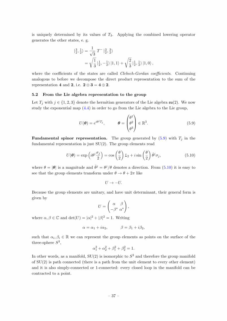
5.2 From the Lie algebra representation to the group
Let Tj with j ∈ 1, 2, 3 denote the hermitian generators of the Lie algebra su(2). We now
study the exponential map (4.4) in order to go from the Lie algebra to the Lie group,
U(θ) = eiθjTj , θ =
θ1
θ2
θ3
∈ R3. (5.9)
Fundamental spinor representation. The group generated by (5.9) with Tj in the
fundamental representation is just SU(2). The group elements read
U(θ) = exp(iθj
σj2
)= cos
(θ
2
)12 + i sin
(θ
2
)θjσj , (5.10)
where θ = |θ| is a magnitude and θj = θj/θ denotes a direction. From (5.10) it is easy to
see that the group elements transform under θ → θ + 2π like
U → −U.
Because the group elements are unitary, and have unit determinant, their general form is
given by
U =
(α β
−β∗ α∗
),
where α, β ∈ C and det(U) = |α|2 + |β|2 = 1. Writing
α = α1 + iα2, β = β1 + iβ2,
such that αi, βi ∈ R we can represent the group elements as points on the surface of the
three-sphere S3,
α21 + α2
2 + β21 + β2
2 = 1.
In other words, as a manifold, SU(2) is isomorphic to S3 and therefore the group manifold
of SU(2) is path connected (there is a path from the unit element to every other element)
and it is also simply-connected or 1-connected: every closed loop in the manifold can be
contracted to a point.
– 37 –

Adjoint or vector representation. If we insert the adjoint representation of Tj in (5.7)
into the exponential map (5.9) one obtains the group elements of SO(3). (Recall that the
Lie algebras so(3) = su(2) agree.) Infinitesimal transformation matrices read
Rmn = δmn + i dθj(Tj)mn = δmn + dθjεjmn. (5.11)
These generate rotations in three-dimensional Euclidean space such that a vector v ∈ R3
transforms under the group action as
vm → v′m = R(θ)mnvn.
From the infinitesimal transformation (5.11) one can easily check that indeed
R(θ)TR(θ) = 13, det(R(θ)) = 1.
Finite versions of the group elements (5.11) can be written as
Rmn = cos(θ)δmn + sin(θ)θjεjmn + (1− cos(θ))θmθn.
One can now check that this is symmetric under θ → θ + 2π,
R→ R.
Limiting the range to θ ∈ (−π, π) we can represent the group elements as points inside of
the closed ball S2 where the antipodal points of the surface are to be identified because
θ = π and θ = −π represent the same group element.
π
•
•
From this consideration we can infer that the group manifold of SO(3) is connected (there
is a path from the unit element to every other element), but it is not simply connected or
1-connected. A loop in the group manifold extending to the boundary that is closed by
going through the antipodal point can not be contracted to a single point. We see here the
even though the Lie algebras of SU(2) and of SO(3) agree, the groups do not. In particular
the topological properties of the group manifolds are actually different.
5.3 Three-dimensional harmonic oscillator
The quantum harmonic oscillator is described by the Hamiltonian
H =p2
2M+
1
2Mω2x2
= ~ω(a†jaj +
3
2
),
– 38 –
where x, p are position and momentum operators respectively, M is the particle’s mass and
ω the angular frequency of the oscillator. The Hamiltonian is then rewritten in terms of
the creation and annihilation operators a†j and aj respectively which obey the commutation
relations
[aj , a†k] = δjk, [a†j , a
†k] = [aj , ak] = 0.
Then the energy eigenstates are
H |n1, n2, n3〉 = ~ω(n1 + n2 + n3 +
3
2
)|n1, n2, n3〉 ,
for nj ∈ N0 where
|n1, n2, n3〉 =
3∏j=1
(a†j)nj√nj !|0〉 .
Define transition operators for the first exited states such that
P12 |1, 0, 0〉 = i |0, 1, 0〉 ,P23 |0, 1, 0〉 = i |0, 0, 1〉 ,P31 |0, 0, 1〉 = i |1, 0, 0〉 .
These states have all the same energy and the operators should Pjk commute with the
Hamiltonian,
[H,Pij ] = 0. (5.12)
One can realize hermitian operators that behave as we want in terms of creation and
annihilation operators,
Pjk = i(a†kaj − a†jak).
In fact, they can be identified with the angular momentum operators
L1 = P23 = x2p3 − x3p2,
L2 = P31 = x3p1 − x1p3,
L3 = P12 = x1p2 − x2p1,
which fulfill the Lie algebra of SU(2),
[Lj , Lk] = iεjklLl.
Equation (5.12) expresses actually angular momentum conservation, [H,Lj ] = 0. Also one
finds
[Lj , a†k] = i εjkl a
†l .
This tells that the operators a†j transform like vectors and thus span the 3 representation of
the Lie algebra of SU(2). One can now also construct higher dimensional representations
by acting several times with the creation operators. Of course, the creation operators
– 39 –

commute, so the result will always be symmetric under the exchange of two of them. The
N ’th excited state transforms as the N -fold symmetric direct product
(3⊗ ...⊗ 3︸ ︷︷ ︸N times
)sym.
We can now decompose any exited level, e.g. the second excited state,
(3⊗ 3)sym = 5⊕ 1,
where the 5 or spin-2 representation is a symmetric and traceless tensor (using Einsteins
summation convention), [1
2a†ja†k +
1
2a†ka†j −
1
3δjka
†l a†l
]|0〉 ,
and similarly the singlet 1 is [a†ja†j
]|0〉 .
The tensor decomposition we are using here is part of a more general decomposition of
a tensor of rank two into three irreducible representations (of the rotation group), namely
a symmetric and trace-less tensor with five independent components, an anti-symmetric
tensor with three independent components, and a trace corresponding to one component,
Tij = T sym, trace-lessij + T anti-sym
ij︸ ︷︷ ︸εijktk
+δijt.
This realizes the tensor product decomposition 3⊗ 3 = 5⊕ 3⊕ 1.
5.4 Bohr atom
As another application we can consider Bohr’s Hamiltonian for the relative motion of the
electron and the proton in a simple hydrogen atom,
H =p2
2M− e2
r.
The spectrum of bound states is given by
En = −Ry
n2,
where n is the principal quantum number, with some degeneracy in the angular momentum
quantum number l = 0, 1, ..., n− 1 and azimuthal quantum number m = −l, ..., 0, ..., l. For
example, the states for n = 2 are in the representations
states with n = 2 :
l = 0 : singlet 0
l = 1 : triplet 3
and have the same energy. The fact that these two states have the same energy poses
the question whether there is a (hidden) symmetry that connects them. We would need a
– 40 –

transition operator from 0 to 3 that commutes with the Hamiltonian. To be in agreement
with rotation symmetry, this transition operator must be vector-like. In classical mechanics
there is the Laplace-Runge-Lenz vector which precisely meets these requirements,
Aclassicali = εijkpjLk −Me2xi
r.
For quantum theory we define it in the hermitian form
Ai =1
2εijk(pjLk + Lkpj)−Me2xi
r,
which obeys
LjAj = AjLj = 0, [Lj , Ak] = iεjklAl,
as well as
[H,Aj ] = 0.
This invariance is a hidden symmetry for 1/r-potentials. We will now use this to find the
spectrum algebraically. We start with the commutation relation
[Aj , Ak] = iεjklLl(−2MH),
and define the rescaled operator
Aj =Aj√−2MH
,
to give the simple commutation relation
[Aj , Ak] = iεjklLl,
as well as
[Lj , Ak] = iεjklAl.
Additionally we know
[Lj , Lk] = iεjklLl.
We define now the linear combinations
X(+)j =
1
2(Lj + Aj),
X(−)j =
1
2(Lj − Aj),
which commute
[X(+)i , X
(−)j ] = 0.
Interestingly, we are now left with two independent copies of the Lie algebra su(2),
[X(+)j , X
(+)k ] = iεjklX
(+)l ,
[X(−)j , X
(−)k ] = iεjklX
(−)l .
– 41 –

We also observe that the quadratic Casimir operators are the same
C(+)2 =
1
4(Lk + Ak)(Lk + Ak) =
1
4(Lk − Ak)(Lk − Ak) = C
(−)2 ,
because of AkLk = LkAk = 0 and therefore
C(+)2 = C
(−)2 = j(j + 1),
where j1 = j2 = j. To express the Hamiltonian in terms of the Casimir operator we
calculate (somewhat lengthy)
AkAk = (−2MH)AkAk =
(p2 − 2Me2
r
)︸ ︷︷ ︸
−2MH
(LkLk + 1) +M2e4,
and arrive at
H = − Me4/2
LkLk + AkAk + 1= − Me4/2
4C(+)2 + 1
= − Me4/2
(2j + 1)2.
In other words, we get the well-known result for the energy spectrum! The principle
quantum number is related to the Casimir by
n = 2j + 1.
To find the degeneracy of these states we note that the angular momentum operator is
given by
Lk = X(+)k +X
(−)k .
For given value of j we have therefore states with different values of angular momentum
as in the direct product representation (2j + 1)× (2j + 1). The possible values for l are
l = 2j = n− 1, l = 2j − 1 = n− 2, . . . , l = 0,
with the usual degeneracy in the quantum number m = −l, ..., l. We have solved the Bohr
atom without a single differential equation!
5.5 Isospin
Fermi-Yang model. Even though protons (mass mp = 938 MeV) carry electromagnetic
charge and neutrons (mass mn = 939 MeV) do not, the small mass difference of the two
particles led to the assumption that this is due to symmetry of the strong interaction.
Assume that nucleons and antinucleons are fermionic states
|p〉 = b†1 |0〉 , |n〉 = b†2 |0〉 ,
|p〉 = b†1 |0〉 , |n〉 = b†2 |0〉 ,
where |0〉 denotes the vacuum state and the creation and annihilation operators satisfy the
anticommutation relations
bi, b†j = bi, b†j = δij ,
– 42 –

with all other anticommutators vanishing. From these operators one can construct three
generators for an su(2) algebra,
Ij =1
2b†α(σj)αβbβ −
1
2b†α(σ∗j )αβ bβ,
as well as one generator for the (rather trivial) Lie algebra of U(1),
I0 =1
2(b†αbα − b†αbα).
The direct product of the two isospin representations 2(p
n
)and
(p
n
)then decomposes according to 2⊗2 = 3⊕1 such that the 3 representation furnishes three
particles,
|π+〉 = b†1b†2 |0〉 , |π0〉 =
1
2(b†1b
†1 − b
†2b†2) |0〉 , |π−〉 = b†2b
†1 |0〉 .
They turn out to have the masses mπ± = 139 MeV and mπ0 = 135 MeV. The pions have
here the same quantum numbers as nucleon-anti-nucleon bound states. As for the proton
and neutron the mass difference is explained by the symmetry breaking when weak and
electromagnetic forces are taken into account. The electro-magnetic charge is given by the
combination
Q = I3 + I0,
where I0 equals 1/2 for nucleons and −1/2 for anti-nucleons. In fact, 2I0 is known as baryon
number, and it is a globally conserved quantum number in QCD. Pions have vanishing
baryon number, I0 = 0.
One may also ask here where the singlet 1 went; one may identify it here with the
η-meson (with mass 548 MeV).
Wigner supermultiplet model. Extending the isospin symmetry by combining it with
spin,
SU(4) ⊃ SU(2)isospin ⊗ SU(2)spin ,
leads to nucleons N and antinucleons N transforming as isospin and spin spinors,
|N〉 ∼ 4 = (2isospin,2spin),
|N〉 ∼ 4 = (2isospin,2spin).
We can now decompose
4⊗ 4 = 15⊕ 1,
and the pions belong to the 15 which now includes also other mesons,
15 = (3isospin,3spin)︸ ︷︷ ︸ρ+, ρ0, ρ−
ρ-meson (vector)1−, 149 MeV
⊕ (1isospin,3spin)︸ ︷︷ ︸ω
ω-meson (vector)1−, 783 MeV
⊕ (3isospin,1spin)︸ ︷︷ ︸π+, π0, π−
pion (scalar)0−
.
– 43 –

The singlet state 1 corresponds again to the scalar η-meson (0−, 548 MeV).
The modern understanding of mesons is not as nucleon-anti-nucleon bound states but
as quark-anti-quark bound states, for example pn ∼ uudddu ∼ ud ∼ π+.
5.6 From SU(2) to the real symplectic group and Bogoliubov transformations
We move now away from the Lie algebra of SU(2) or SO(3) and broaden the view some-
what. Consider the quantum mechanical commutation relation between position x and
momentum p,
[x, p] = i,
In terms of the combined variable
q =
(x
p
),
the commutation relation can be rewritten as
[qj , qk] = iΩjk,
with the antisymmetric matrix
Ω = iσ2 =
(0 +1
−1 0
).
One may consider canonical transformations
qj → q′j = qmSmj , (5.13)
such that
[q′j , q′k] = SmjSnk[qm, qn] = i STjmΩmnSnk = iΩjk.
In other words, the canonical commutation relation should remain unmodified. This leads
to the condition
STΩS = Ω, (5.14)
which characterizes the symplectic group Sp(2,R). (We do not allow complex transforma-
tions because we want qj to remain real, or hermitian as an operator.) As usual we write
the group element in exponential form,
S = exp(iθjTj
).
The Lie algebra elements of Sp(2,R) are subject to ΩT = (ΩT )T . We can take
T1 = −i12σ1, T2 =
1
2σ2, T3 = −i1
2σ3. (5.15)
such that ΩTj = iσ2Tj are symmetric and iTj are real matrices. Note that the basis (5.15)
is obtained from the basis (5.4) for su(2) by multiplying two generators with −i. This has
an important consequence for the quadratic Casimir, which becomes now
C2 = −T 21 + T 2
2 − T 23 , [C2, Tj ] = 0. (5.16)
– 44 –

This is not positive semi-definite any more! This means that for a given value of C2, the
spectrum of the Tj does not need to be bounded and indeed, many representations of the
Lie algebra (5.15) are actually infinite.
The group matrices themselves can be written as
S =
(s11 s12
s21 s22
)and from (5.14) we find the condition s11s22 − s12s21 = 1. The matrix entries smn are real
but not bounded. The group manifold of Sp(2,R) is not compact. This is closely related
to the fact that C2 is not positive semi-definite.
One can use symplectic transformations to rewrite quadratic expression of the form
(with ∆12 = ∆21)
1
2(x, p)
(∆11 ∆12
∆21 ∆22
)(x
p
)=
1
2qT∆ q =
1
2q′TS∆ST q′ =
1
2q′T∆′q′, (5.17)
with q = ST q′ and
∆′ = S∆ST .
Note that this is not a standard similarity transform because ST 6= S−1. Nevertheless, one
can make some general statements about such symplectic transformations and in particular
according to Williamsons theorem1 one can here find an S such that ∆′ = diag(λ, λ) is
diagonal with two equal eigenvalues. In that case, the expression on the right hand side
of (5.17) becomes just the Hamiltonian of a harmonic oscillator, λ2 (x′2 + p′2). In other
words, symplectic transformations can be used to simplify Hamiltonians that are quadratic
in variables and their conjugate momenta and in order to bring them to a simple standard
form.
One can also relate the symplectic transformations (5.13) to transformations between
creation and annihilation operators(a
a†
)→
(b
b†
)=
(u v
v∗ u∗
)(a
a†
), (5.18)
where u, v ∈ C. Then
[b, b†] = [ua+ va†, v∗a+ u∗a†] = (|u|2 − |v|2)[a, a†],
and thus for |u|2 − |v|2 = 1 the transformation is canonical (it preserves the canonical
commutation relation) and known as a Bogoliubov transformation.
Also, the form of the quadratic Casimir in (5.16) suggests a relation to the indefinite
orthogonal group SO(2, 1) of Lorentz transformations in d = 2 + 1 dimensions, which is
also not compact. This can indeed be established, as well.
[Exercise: Find the relation between real symplectic transformations and Bogoliubov
transformations. Also establish a relation between Sp(2,R) and indefinite orthogonal trans-
formations SO(2, 1).]1This theorem states that a real symmetric positive definite matrix of even dimension can be brought
to diagonal form by a symplectic congruence transformation. The diagonal entries come in pairs and are
called symplectic eigenvalues.
– 45 –

6 Matrix Lie groups and tensors
Now that we understood the Lie algebra of the simplest unitary and orthogonal groups up
to SU(2) and of SO(3), and before moving on to SU(3), let us pause for a moment and
explore what can be said about general matrix Lie groups GL(N,C) and specifically about
the groups SO(N) and SU(N) and their tensor representations on general grounds.
6.1 General linear group GL(N,C)
Quite generally, a matrix Lie group has a fundamental representation of the form
vj →M jkvk.
Here M could be an element of the orthogonal group O(N) for example, but also any other
matrix Lie group. In this subsection we make only the minimal assumption M ∈ GL(N,C).
One can then immediately build higher rank tensor representations that transform like
vjn···p →M jkM
nm · · ·Mp
q vkm···q.
It is also convenient to introduce representations with lower index, which should transform
like
wj → (M−1)kjwk. (6.1)
Now one can contract upper and lower indices to yield an invariant term, for example,
wjvj → (M−1)mjM
jkwmv
k = δmkwmvk = wkv
k.
A general tensor can now have upper and lower indices and transforms accordingly, for
example,
vjn →M jk (M−1)mnv
km.
In other words, upper indices transform with M , lower indices transform with the inverse
M−1. The unit tensor with one upper and one lower transforms like
δjn →M jk (M−1)mnδ
km = M j
m (M−1)mn = δjn.
One may say that δjn is an invariant symbol. In contrast, δmn or δmn are in general not
invariant.
To find another invariant symbol consider also the N -dimensional Levi-Civita symbol
εijk···n. It is totally antisymmetric, which means anti-symmetric in any pair of indices,
ε···k···m··· = −ε···m···k···, (6.2)
and normalized such that
ε123···N = 1. (6.3)
Under the matrix group it transforms to
εijk···n →M ipM
jq · · ·M
nsεpq···s = det(M)εij···n.
This shows that for the special linear group M ∈ SL(N,C) where det(M) = 1 the Levi-
Civita symbol εijk...n is also an invariant symbol. Similarly, an analogously defined Levi-
Civita symbol with lower indices εijk···n is also invariant for det(M) = 1.
– 46 –

6.2 Orthogonal group SO(N)
The group of rotations in N -dimensional Euclidean space is SO(N) where the group ele-
ments are N ×N matrices R (in the fundamental representation) satisfying
RTR = RRT = 1, or RjmRknδmn = δjk, (6.4)
and
det(R) = 1. (6.5)
This is clearly a subgroup of SL(2,R). A vector in the sense of rotations is defined by its
transformation behavior under rotations, namely
vj → Rjk vk.
This constitutes obviously a representation of the group SO(N). Analogously we define
tensors be to objects transforming like
vij → RimRjnv
mn, (6.6)
and so on for higher rank tensors. To be complete, a scalar transforms in the trivial way,
s→ s.
Interestingly, SO(N) has more invariant symbols then GL(N) or SL(N). Specifically,
the defining property in eq. (6.4) tells that
δjk → RjmRknδmn = δjk,
and similarly δjk, are also invariant symbols. These two can now be used to raise and
lower indices so that one does not really need to distinguish upper and lower indices for
SO(N). For the rest of the discussion in this subsection we will only use lower indices for
this reason.
One may ask whether the tensor representation (6.6) can de decomposed into different
parts that do not mix under rotations, i. e. whether the representation is reducible. This
is indeed the case.
The anti-symmetric combination
Aij =1
2(Mij −Mji) = −Aji,
again is a tensor and it also does not mix with other parts under rotations. There are
N(N−1)/2 independent components for anti-symmetric second-rank tensors. Analogously
we can argue for a symmetric second-rank tensor
Sij =1
2(Mij +Mji),
which has N(N + 1)/2 independent components. The trace is actually a scalar because
Sjj → RjkRjlSkl = (RT )kjRjlSkl = δklSkl = Skk.
– 47 –

Constructing the symmetric and trace-less second-rank tensor
Sij = Sij − δijSkkN
,
we are left with N(N + 1)/2 − 1 components. Therefore we have decomposed the tensor
representation into three irreducible representations,
N⊗N =
[N(N− 1)
2
]⊕[N(N + 1)
2− 1
]⊕ 1.
For example for SO(3) this gives 3⊗ 3 = 5⊕ 3⊕ 1 as we have seen before. For a general
decomposition of higher rank tensors Mijk...m the technique of Young tableaux was invented
to keep track of the emerging patterns. We will not discuss this further here, however.
Dual tensors. Let Aij be an anti-symmetric second-rank tensor. We define its dual to
be the totally anti-symmetric (N − 2)-rank tensor
Bk...n = εijk...nAij .
For example, for N = 3 we get in this way a vector
Bk = εijkAij ,
and for N = 2 a scalar
B = εijAij .
In the case of N = 4 we again get a relation between two anti-symmetric second-rank
tensors as it is used in electromagnetism, namely the fields strength tensor and its dual in
4-dimensional Euclidean space (for the treatment in Minkowski space we are dealing with
SO(3, 1) not SO(4) anymore),
Bkl = εijklAij .
Self-dual / Anti-self-dual tensors. For an even number of dimensions, i. e. for SO(2n)
we can construct two irreducible representations with an additional feature. Consider an
totally anti-symmetric n-rank tensor Ai1i2...in and its dual,
Bi1i2...in =1
n!εi1i2...inj1j2...jnAj1j2...jn ,
such that
Ai1i2...in =1
n!εi1i2...inj1j2...jnBj1j2...jn .
In other words, the two tensors A and B are dual to each other. We can form the linear
combinations
M±i1...in =1
2(Ai1...in ±Bi1...in),
and they are self-dual and anti-self-dual. This can be seen by writing schematically
εM± =1
2(εA± εB) = ±1
2(A±B) = ±M±.
The self-dual and anti-self-dual tensors are also each irreducible representations of the
rotation group SO(N).
– 48 –

6.3 Unitary group SU(N)
Now that we have discussed SO(N), let us move to the unitary group SU(N). For SU(N)
we write the fundamental representation as
ψj → U jkψk. (6.7)
The complex conjugate spinor transforms then formally like
ψ∗j → (U jk)∗ψ∗k.
However, we also have the transformation law for a lower index spinor,
ξj → (U−1)kjξk = (U †)kjξk. (6.8)
The matrix elements of (U jk)∗ and (U †)kj are actually identical so that we can simply and
consistently write complex conjugate spinors with a lower index,
(ψj)∗ = ψ∗j .
This has the nice feature that the quadratic form ξ†ψ = ξ∗jψj transforms like
ξ∗jψj → ξ∗j (U †)kjU
jmψ
m = ξ∗j δjmψ
m = ξ∗jψj ,
so it is invariant as expected. One can now also consider tensors with several upper and
lower indices and transform them consistently, for example
φijk → U ilUjm(U †)nk φ
lmn.
It is important to note that δjk and δmn are not invariant symbols any more. [Exercise:
Check this!] They can accordingly also not be used to raise or lower indices. This means
that one must indeed be careful to distinguish upper and lower indices for SU(N).
We can sometimes use the fully anti-symmetric Levi-Civita symbol εij···n introduced in
eqs. (6.2) and (6.3) and its counterpart εij···n to raise and lower indices. This works because
the elements of SU(N) have unit determinant. For example for SU(4) we can lower indices
of a tensor ϕ ijk that is anti-symmetric in i and j and define a new tensor with only lower
indices as φkpq = εijpq ϕijk .
In case of SU(2) there is a special situation because the invariant symbols εij and εij
allow to pull all indices up or all indices down, e. g.
ψm = εmjψj .
This also implies that there is no real difference between the fundamental representation
and its complex conjugate. This can also be understood directly from the exponential map
U = exp(iθj
σj2
).
The complex conjugate of the Pauli matrices can be written as (recall eq. (5.5))
σ∗j = −S−1σjS,
– 49 –

where S is given by
S = −iσ2 =
(0 1
−1 0
).
Note that the matrix entries of S agree with the Levi-Civita symbol, Sjk = εjk. The group
element U and its complex conjugate U∗ are related through
U∗ = exp
(−iθj
σ∗j2
)= S−1 exp
(iθj
σj2
)S = S−1US,
which is just a similarity transform. Such a simple relation between a representation and its
complex conjugate is not available for N > 2, though. In general, for a given representation
of SU(N) with multiplication law
U1U2 = U3,
we can obtain another representation by taking complex conjugates.
U∗1U∗2 = U∗3 ,
While the fundamental representation itself is for a spinor ψj as in (6.7), the complex
conjugate representation is for a lower index spinor ξj as in (6.8).
– 50 –

7 SU(3)
7.1 Lie algebra
We now consider the Lie algebra of SU(3). The vector space of hermitian and trace-less
3 × 3 matrices is spanned by the Gell-Mann matrices. Their role is similar to the role
played by the Pauli matrices for SU(2). The Gell-Mann matrices can be taken as
λ1 =
0 1 0
1 0 0
0 0 0
, λ2 =
0 −i 0
i 0 0
0 0 0
, λ3 =
1 0 0
0 −1 0
0 0 0
,
λ4 =
0 0 1
0 0 0
1 0 0
, λ5 =
0 0 −i0 0 0
i 0 0
,
λ6 =
0 0 0
0 0 1
0 1 0
, λ7 =
0 0 0
0 0 −i0 i 0
, λ8 =1√3
1 0 0
0 1 0
0 0 −2
.
They are normalised to Trλaλb = 2δab. Observe that the first three Gell-Mann matrices
contain the Pauli matrices, (λ1, λ2, λ3) ∼ (σ1, σ2, σ3), acting on a subspace. They can be
used to construct an su(2) subalgebra.
We can now investigate the other commutators and because λ3 and λ8 are diagonal
we immediately find
[λ3, λ8] = 0.
Moreover we introduce a new matrix λ[4,5] by
2iλ[4,5] = [λ4, λ5] = 2i
1 0 0
0 0 0
0 0 −1
= i(λ3 +√
3λ8),
and therefore λ4, λ5, λ[4,5] work similarly as the Pauli matrices but now in the 1-3-sector.
They can also be used to span an su(2) algebra. Something similar can also be done in the
2-3-sector with λ6, λ7 and λ[6,7] defined through
2iλ[6,7] = [λ6, λ7] = 2i
0 0 0
0 1 0
0 0 −1
= i(−λ3 +√
3λ8).
In total we find three overlaping copies of the su(2) algebra.
The Lie algebra su(3) is generated in the fundamental representation by
Tj =λj2.
In the light of the above discussion we define six new operators
I± = T1 ± iT2, V± = T4 ± iT5, U± = T6 ± iT7. (7.1)
– 51 –

Note that I†± = I∓ and similar for V± and U±. The operators in eq. (7.1) form a basis of
the Lie algebra together with the commuting diagonal generators T3 and T8, [T3, T8] = 0.
One finds the commutation relations
[T3, I±] = ±I±, [T3, U±] = ∓1
2U±, [T3, V±] = ±1
2V±,
[T8, I±] = 0, [T8, U±] = ±√
3
2U±, [T8, V±] = ±
√3
2V±,
[I+, I−] = 2T3, [U+, U−] =√
3T8 − T3, [V+, V−] =√
3T8 + T3,
[I+, V−] = −U−, [I+, U+] = V+, [U+, V−] = I−,
[I+, V+] = 0, [I+, U−] = 0, [U+, V+] = 0.
For su(3) we have two Casimir operators, one quadratic,
C2 =
8∑j=1
T 2j ,
and one cubic
C3 =
8∑j,k,l=1
fjklTjTkTl.
Here fjkl are the structure constants, defined through the commutation relation
[Tj , Tk] = ifjkl Tl. (7.2)
Because there are now two Casimir operators there are also two labels. We can label the
states in every irreducible representation by eigenstates of T3 and T8,
|i3, i8〉 ,
such that
T3 |i3, i8〉 = i3 |i3, i8〉 , T8 |i3, i8〉 = i8 |i3, i8〉 .
One can then verify that
T3I± |i3, i8〉 = (I±T3 ± I±) |i3, i8〉 = (i3 ± 1)I± |i3, i8〉 ,T8I± |i3, i8〉 = I±T8 |i3, i8〉 = i8I± |i3, i8〉 ,
and thus
I± |i3, i8〉 ∝ |i3 ± 1, i8〉 .
Analogously
T3U± |i3, i8〉 =(i3 ∓ 1
2
)U± |i3, i8〉 ,
T8U± |i3, i8〉 =(i8 ±
√3
2
)U± |i3, i8〉 ,
giving
U± |i3, i8〉 ∝ |i3 ∓ 12 , i8 ±
√3
2 〉 ,
and finally in the same manner
V± |i3, i8〉 ∝ |i3 ± 12 , i8 ±
√3
2 〉 .
– 52 –

Root vectors. We can summarize these relations diagrammatically. On a lattice spanned
by i3 and i8 the operators I±, V± and U± can be represented as follows.
i3
i8
I+I−
U+
U−
V+
V−
The vectors appearing here are called root vectors,
I± = (±1, 0) , U± =(∓1
2 ,±√
32
), V± =
(±1
2 ,±√
32
).
The root vectors associated to T3 and T8 are (0, 0) because these operators do not change
the labels. We can make a few observations.
• Root vectors have unit lengths or vanish.
• The angles between them are π3 , 2π
3 and so on.
• In some cases the sum of two root vectors gives another root vector, in some not.
• The sum of a root vector with itself is not a root vector.
Positive roots and simple roots. We define positive roots to be characterised by i3 > 0.
Therefore V+, I+ and U− are positive while V−, I−, and U+ are negative. Moreover, among
the positive roots there is a linear relation
I+ = V+ + U−,
and V+ as well as U− are called the simple roots.
7.2 Representations
Weight diagrams and fundamental representation. Let R be some (irreducible or
reducible) representation of su(3) and plot the states |i3, i8〉 in the i3, i8 plane. For the
fundamental representation 3 we identify the states with quark states,
|u〉 = |12 ,1
2√
3〉 ,
|d〉 = |−12 ,
12√
3〉 ,
|s〉 = |0,− 1√3〉 .
The weight diagram is as follows.
– 53 –

i3
i8
strangeness
−12
12
12√
3
− 1√3
0
−1
•u•d
isospin
•s
Using the root vectors we see that
V− |u〉 ∝ |s〉 , V+ |s〉 ∝ |u〉 ,I− |u〉 ∝ |d〉 , I+ |d〉 ∝ |u〉 ,U+ |s〉 ∝ |d〉 , U− |d〉 ∝ |s〉 ,
as well as (for example)
V+ |u〉 = I+ |u〉 = U+ |u〉 = U− |u〉 = 0.
Charge or complex conjugation. Let us investigate how the generators behave under
charge or complex conjugation,
TCj = −T ∗j = −T Tj .
Here we used that the generators are hermitian. From the commutation relation (7.2) we
find also
[TCj , TCk ] = ifjkl T
Cl .
This is something we have observed before: for every representation of SU(3) there is also
a complex conjugate representation. Concretely we find from the Gell-Mann matrices
TCj = Tj ,
for j = 2, 5, 7 and
TCj = −TCj
for j = 1, 3, 4, 6, 8. Thus we conclude for the charge conjugate
C |i3, i8〉 = |−i3,−i8〉 .
– 54 –

Charge conjugate representation. We are now ready to look at the charge conjugate
representation 3∗ where we identify the states as the antiparticles of the 3 states, namely
|u〉 = |−12 ,−
12√
3〉 ,
|d〉 = |12 ,−1
2√
3〉 ,
|s〉 = |0, 1√3〉 .
The weight diagram is now
i3
i8
−12
12
1√3
− 12√
3
•u
•d
•s
Singlet representation. For the singlet representation 1 the weight diagram is almost
trivial with only one state (i3, i8) = (0, 0).
i3
i8
•
Adjoint representation. In the adjoint representation we have
adj(Tj)X = [Tj , X],
with X = XjTj being a linear combination of generators itself. This satisfies the algebra
because
[adj(Tj), adj(Tk)]X = adj([Tj , Tk])X
is equivalent to
[Tj , [Tk, X]]− [Tk, [Tj , X]] = [[Tj , Tk], X]
or
[Tj , [Tk, Tl]] + [Tk, [Tl, Tj ]] + [Tl, [Tj , Tk]] = 0.
– 55 –

This is simply the Jacobi identity.
The weight table for the adjoint representation 8 can be computed using the commu-
tation relations.
state [T3, V ] [T8, V ] weight (i3, i8)
T3 0 0 (0, 0)
T8 0 0 (0, 0)
I+ +1 0 (+1, 0)
I− −1 0 (−1, 0)
U+ −12 +
√3
2 (−12 ,+
√3
2 )
U− +12 −
√3
2 (+12 ,−
√3
2 )
V+ +12 +
√3
2 (+12 ,+
√3
2 )
V− −12 −
√3
2 (−12 ,−
√3
2 )
The weight diagram is now as follows.
i3
i8
•T3 •
T8 •I+
•V+•
U+
•I−
•V−
•U−
Tensor product representations. Analogous to what we have done for SU(2) we can
consider tensor product representations out of representations T(1)k and T
(2)k with states
|i3, i8〉(1) and |j3, j8〉(2) respectively. (We drop the indices (1) and (2) when no confusion
can arise.) Define
Tk = T(1)k + T
(2)k ,
and we have for example
T3 |i3, i8〉 |j3, j8〉 =(T
(1)3 + T
(2)3
)|i3, i8〉 |j3, j8〉 = (i3 + j3) |i3, i8〉 |j3, j8〉 .
A difference to SU(2) is that we now have two labels for SU(3). The Lie algebra su(3) is
rank two. Let us denote
Em+ = I+, U+, V+,Em− = I−, U−, V−,
where m = 1, 2, 3 and study 3⊗ 3. The weight table is as follows.
– 56 –

state weight (i3, i8)
u⊗ u (1, 1√3)
d⊗ d (−1, 1√3)
s⊗ s (0,− 2√3)
u⊗ d, d⊗ u (0, 1√3)
u⊗ s, s⊗ u (12 ,−
12√
3)
d⊗ s, s⊗ d (−12 ,−
12√
3)
We can represent these in the following weight diagram.
i3
i8
•dd •du •ud •uu
•ds •sd •su •us
•ss
For the highest weight state we need Em+ |s〉 = 0 and therefore it is u ⊗ u. Applying
Em− |u⊗ u〉 generates the representation 6 with the following weight table.
state weight (i3, i8)
u⊗ u (1, 1√3)
d⊗ d (−1, 1√3)
s⊗ s (0,− 2√3)
1√2(u⊗ d+ d⊗ u) (0, 1√
3)
1√2(u⊗ s+ s⊗ u) (1
2 ,−1
2√
3)
1√2(d⊗ s+ s⊗ d) (−1
2 ,−1
2√
3)
Accordingly this representation 6 has the following weight diagram.
– 57 –

i3
i8
• • •
• •
•
The remainder of the decomposition is 3∗ with the weight table
state weight (i3, i8)1√2(d⊗ u− u⊗ d) (0, 1√
3)
1√2(d⊗ s− s⊗ d) (−1
2 ,−1
2√
3)
1√2(s⊗ u− u⊗ s) (1
2 ,−1
2√
3)
and weight diagram
i3
i8
•
• •
We have thus decomposed 3⊗ 3 = 6⊕ 3∗ where 3∗ denotes the charge conjugate. Similar
one can derive the weight tables and diagrams for 3∗ ⊗ 3∗ = 6∗ ⊕ 3. Now for 3⊗ 3∗. The
weight table is
state weight (i3, i8)
u⊗ u, d⊗ d, s⊗ s (0, 0)
u⊗ s (12 ,√
32 )
u⊗ d (1, 0)
d⊗ s (−12 ,√
32 )
d⊗ u (−1, 0)
s⊗ u (−12 ,−
√3
2 )
s⊗ d (12 ,−
√3
2 )
– 58 –

and the associated weight diagram
i3
i8
•ds •us
•du •uu •dd•ss
•ud
•su •sd
Applying lowering operators to the highest weight state u⊗ s give the states
u⊗s , u⊗d , d⊗s , d⊗u , s⊗u , s⊗d , 1√2
(d⊗d−u⊗u) ,1
2(d⊗d+u⊗u−2s⊗s)
which furnish the 8 representation with the following weight diagram
i3
i8
• •
• •• •
• •
There is a singlet representation left with the state 1√3(u ⊗ u + d ⊗ d + s ⊗ s). It is clear
that this must be a singlet because it is annihilated by all raising or lowering operators
Em± . Thus we have decomposed 3⊗ 3∗ = 8⊕ 1. Finally considering 3⊗ 3⊗ 3 the weight
table can be derived analogously and the weight diagram is
– 59 –

i3
i8
•ddd •••ddu •••duu •uuu
•••dds ••••••dus
•••uus
•••dss •••uss
•sss
In the exact same way as before applying lowering operators to the highest weight state
(uuu) we can decompose 3⊗ 3⊗ 3 = 10⊕ 8⊕ 8⊕ 1. The first irreducible representation
are the symmetric combinations
u⊗ u⊗ u , d⊗ d⊗ d , s⊗ s⊗ s , 1√3
(u⊗ u⊗ s+ u⊗ s⊗ u+ s⊗ u⊗ u) , ...
forming 10 whereas the singlet 1 is the totally anti-symmetric combination
1√6
(s⊗ d⊗ u− s⊗ u⊗ d+ d⊗ u⊗ s− d⊗ s⊗ u+ u⊗ s⊗ d− u⊗ d⊗ s).
The octet states have mixed symmetry.
7.3 Meson and baryon states
One can now assign particle states to the derived decomposed representations, namely
mesons to the decomposition
3⊗ 3∗ = 8⊕ 1,
and baryons to
3⊗ 3⊗ 3 = 10⊕ 8⊕ 8⊕ 1.
We use the following quantum numbers
• B: baryon number
• S: strangeness (number of s quarks − number of s quarks)
• J : spin
• I3: isospin (actually the third component of it)
• Y = B + S: hypercharge.
– 60 –

We then identify the pseudoscalar mesons (B = 0, J = 0) with the weight diagram 8
I3
Y = B + S
•η•π
0
•π+
•K+
•K0
•π−
•K−
•K0
495 MeV
137 MeV549 MeV
495 MeV
and the additional singlet with the η′-particle. Note that the pion triplet and the η meson
appear here again, now as part of a larger structure. One observes that SU(3) symmetry is
actually broken to some extend, otherwise all the states in 8 would have the same masses.
This breaking is mainly due to the somewhat larger mass of the strange quark compared
to the lighter up and down quarks.
Analogous for the vector mesons (B = 0, J = 1) with weight diagram
I3
Y = B + S
•ω•ρ0
•ρ+
•K+∗
•K0∗
•ρ−
•K−
∗ •K0∗
892 MeV
770 MeV783 MeV
892 MeV
and the additional singlet is the φ-particle.
The baryons (B = 1, J = 32) are in the 10 representation with the weight diagram
– 61 –

I3
Y = B + S
•∆−
•∆0
•∆+
•∆++
•Σ−∗
•Σ0∗•Σ+∗
•Ξ−∗
•Ξ0∗
•Ω−
1235 MeV
1385 MeV
1530 MeV
1670 MeV
In contrast the baryons (B = 1, J = 12) form an 8 with weight diagram
I3
Y = B + S
•Σ0
•Λ0
•Σ+
•p
•n
•Σ−
•Ξ−
•Ξ+
939 MeV
1193 MeV1116 MeV
1318 MeV
Interestingly, the neutron and proton now appear as part of a larger structure which in-
cludes other, somewhat heavier baryons.
Now the question might arise why there are no 3⊗ 3 or 3⊗ 3⊗ 3∗ states. The reason
is related to another SU(3) symmetry of quarks that we did not discuss so far: color. One
assumes that all observable / asymptotic states are singlets with respect to an additional
SU(3)C colour symmetry. Because we have
3C ⊗ 3∗C = 8C ⊕ 1C ,
as well as
3C ⊗ 3C ⊗ 3C = 10C ⊕ 8C ⊕ 8C ⊕ 1C ,
there are singlets under SU(3)C in both cases. In contrast,
3C ⊗ 3C = 6C ⊕ 3∗C ,
– 62 –

does not contain any color singlets. This is the reason why no states from 3C ⊗ 3C can be
observed.
7.4 Nucleon-meson models
Let us turn again to the isospin model of the Lie algebra of SU(2) in the fundamental
representation we already encountered and denote the nucleons and antinucleons as
N i =
(p
n
), Ni =
(p
n
).
Their transformation in the notation we have established for general SU(N) then is
N i → U ijNj , Ni → Nj(U
†)ji.
Turning to the adjoint representation we can write
φ = π · σ = π1σ1 + π2σ2 + π3σ3
=
(π3 π1 − iπ2
π1 + iπ2 −π3
)=
(π0
√2π+
√2π− −π0
),
which transforms under SU(2) like
φij → φ′ij = U il φ
lm (U †)mj .
In other words, the pions are now forming a matrix valued field! We now use these fields
to construct an invariant Lagrangian. For example, an interaction term of the form
L = ...+ gNiφijN
j ,
is SU(2) invariant. Explicitly, we can expand(p, n
)( π0√
2π+√
2π− −π0
)(p
n
)= pπ0p− nπ0n+
√2pπ+n+
√2nπ−p.
The appearing terms can be expressed in terms of Feynman diagrams.
t
p
•gp
π0
p
•g
p
n
•−g
nπ0
n
•−g n
p
•√2g
nπ+
n
•√
2g p
In a similar manner one may also introduce a meson field as an adjoint representation
of SU(3),
φ =1√2
8∑a=1
φaλa =
1√2π0 + 1√
6η π+ K+
π− − 1√2π0 + 1√
6η K0
K− K0 − 2√6η
.
– 63 –

Besides the pions this includes now also the Kaons and the η meson. We may start by
assuming a Lagrangian with full SU(3) symmetry
L0 =1
2gµν Tr (∂µφ)(∂νφ) − 1
2m2
0 Trφφ.
Here all mesons masses would be equal, which clearly is not the case and therefore we have
to introduce a term that break the symmetry. Suppose we have a symmetric Hamiltonian
H0 and introduce a perturbation H1 which breaks the symmetry,
H = H0 + αH1.
As long as α stays small we are in the perturbative regime such that H1 just shifts the
energy eigenvalue by a small amount
〈s|H0|s〉 = Es,
〈s|αH1|s〉 = ∆E.
We can therefore write
E = Es + ∆E +O(α2).
Let us now try to find a suitable symmetry breaking term in the Lagrangian. It is
natural to search for a term quadratic in the fields, so we need to use the decomposition
8⊗ 8 = 27⊕ 10⊕ 10∗ ⊕ 8⊕ 8⊕ 1,
As usual, these terms can be split into symmetric and anti-symmetric terms,
(8⊗ 8)s = 27⊕ 8⊕ 1,
(8⊗ 8)a = 10⊕ 10∗ ⊕ 8.
We need to concentrate here on the symmetric terms because mesons are bosonic and φ2
is symmetric in this sense. The singlet 1 from the first line is actually the mass term in
L0. For the breaking term we can choose between 27 and 8. It is probably natural to start
with the simpler case so we pick 8 and add a term ∼ Trφφλ8 as the breaking term.
Note that we need to preserve the isospin SU(2) in the upper part of φ to keep the
pion structure. Now we decompose the Gell-Mann matrix λ8 into two parts,
λ8 =1√313 −
2√3
0 0 0
0 0 0
0 0 1
,
such that the first term adds to the mass term in the Lagrangian and the second is new.
It breaks the SU(3) symmetry in the right way, namely
Tr
φφ0 0 0
0 0 0
0 0 1
= K−K+ +K0K0 +
2
3η2,
– 64 –

and therefore we can write the perturbed Lagragian as
L = L0 −1
2κ
[K−K+ +K0K0 +
2
3η2
].
The new term corrects the mass term of the kaons and the η-meson but not of the pion.
This needs to be compared to the mass term in the unperturbed Lagrangian,
Trφφ = (π0)2 + η2 + 2K−K+ + . . . .
To first order in perturbation theory around the symmetric situation one finds
m2π = m2
0, m2η = m2
0 +2
3κ, m2
K = m20 +
1
2κ,
which yields the Gell-Mann Okubo mass formula
4m2K = 3m2
η +m2π.
Indeed this is fulfilled to reasonably good accuracy.
[Exercise: Di-quarks are hypothetical bound states of two quarks (but no anti-quarks).
Because they necessarily carry color, they cannot be asymptotic states but might arise
as resonances. Moreover, it may be possible to understand baryons as bound states of
di-quarks with an additional quark. Using your freshly gained insights into SU(3) repre-
sentation theory, classify the di-quarks states composed out of the up, down, and strange
quarks 3 ⊗ 3 with respect to their transformation behaviour under SU(3) and the color
symmetry SU(3)C .]
– 65 –

8 Classification of compact simple Lie algebras
In the following we will briefly go through a classification of Lie algebras worked out by
Wilhelm Killing and Elie Cartan. This topic is treated in much more depth in mathematics
lectures and books; we can only cover the very basics here. More specifically, in this
section we will discuss a general classification of a special class of real Lie algebras, namely
those that are simple and for which the corresponding Lie group is compact as a manifold.
However, this is the basis also for other cases. Let us first clarify these notions.
Simple Lie group and algebra. Recall that we defined finite simple groups as those
that do not have any non-trivial normal subgroups and that other finite groups could be
reduced to those. Recall also that a subgroup H of G was called normal when ghg−1 ∈ Hfor all h ∈ H and g ∈ G. For Lie groups one can define similarly: a simple Lie group
is a connected, non-abelian Lie group which does not have non-trivial connected normal
subgroups. (Note as an aside that it may have discrete normal subgroups.) One can also
express this through the algebra: a simple Lie group is a connected Lie group for which
the corresponding Lie algebra is simple. A simple Lie algebra in turn is a Lie algebra that
is non-abelian and that does not contain any non-trivial ideal. To understand this, we also
need the following notions.
Lie subalgebra and ideal. A Lie subalgebra is a sub vector-space of the Lie algebra
that is also closed with respect to the Lie bracket. In other words, the Lie bracket of two
elements of the subalgebra is again an element of the subalgebra. An ideal in this context
is a Lie subalgebra that fulfills the stronger condition that the Lie bracket of any element
of the full Lie algebra with an element of the ideal is again part of the ideal.
Semi-simple Lie algebra. A semi-simple Lie algebra is a Lie algebra that can be written
as a direct sum of simple Lie algebras. In other words, semi-simple Lie algebras can be
composed out of simple Lie algebras.
By the so-called Levi decomposition one can actually decompose all finite dimensional
real or complex Lie algebras in terms of a semi-simple Lie subalgebra and a solvable Lie
algebra for which an abelian Lie algebra is an example. We see here that simple Lie algebras
are an important building block to understand the general case.
Compact Lie group and algebra. A Lie group is called compact if it is compact as
a manifold. (For example the rotation group in four dimensions SO(4) is compact, but
the group of special Lorentz transformations SO(1, 3) is not.) Accordingly, one calls a Lie
algebra compact if it is the Lie algebra of a compact group. This is of course not the general
case. However, it turns out that both compact and non-compact simple real Lie algebras
can be seen as restrictions, so-called real forms, of the same simple Lie algebras over the
complex numbers and for every such complex simple Lie group there is a particular real
form that is compact. In this sense, studying the compact real Lie algebras gives insights
into the general case. As a physicist one would say that compact and non-compact Lie
algebras (and their groups) are related through analytic continuation. (For example Wick
rotation from SO(1, 3) to SO(4).)
– 66 –

8.1 The adjoint representation
Previously we have already introduced the adjoint representation for the Lie algebra. Now
we also discuss the adjoint representation of the group. The interesting thing about the
adjoint representation is that we need no additional structure; everything is provided by
the Lie group already. Consider a group element h ∈ G on which other group elements
g ∈ G act as follows
h→ Adg(h) = ghg−1.
This is obviously a representation of the group, in the sense that Adg1(Adg2(h)) = Adg1g2(h).
Note that this representation acts in fact in the group space itself, because h is simply a
group element. However, one may also take h to be infinitesimally close to the unit element,
h = 1+ iζjTj , and finds
h = 1+ iζkTk → ghg−1 = 1+ ig(ζkTk)g−1.
This shows that one may also consider the adjoint representation to act on the space of
the Lie algebra,
ζkTk → g(ζkTk)g−1.
Finally, we may take also g to be infinitesimal, g = 1+ iξjTj , and find to linear order in ξj ,
ζkTk → g(ζkTk)g−1 = ζkTk + i
[ξjTj , ζ
kTk
]= ζ ′kTk. (8.1)
We can identify the representation of the Lie algebra in the adjoint representation as acting
in terms of the commutator. Now we can express the Lie bracket in term of the structure
constants as
[Tj , Tk] = if ljk Tl. (8.2)
It is clear from (8.2) that the structure constants are anti-symmetric in the first two indices,
f ljk = −f l
kj . Let us also recall that they are real, f ljk ∈ R, for Lie algebras with some
hermitian representation T †j = Tj . This is the case for the Lie algebras of compact Lie
groups.
Eq. (8.2) allows to write the infinitesimal transformation in the adjoint representation
(8.1) as
ζk → ζ ′k =[δkl + iξj(T
(A)j )kl
]ζ l, (8.3)
with the Lie algebra generators in the adjoint representation introduced already in (4.13)
(T(A)j )kl = i f k
jl . (8.4)
It follows from the Jacobi identity in eq. (4.11) that these matrices satisfy also the com-
mutation relation (8.2). Note that we are carefully distinguishing upper and lower indices
here. As it is defined in (8.3), the adjoint representation acts on the Lie algebra or the
tangent space of the Lie group at the position of the identity element.
– 67 –

Note that (8.3) can be understood as a matrix representation of the Lie algebra. As
usual, an object with a lower index (actually an element of the co-tangent space or a
one-form) transforms with the inverse matrix,
ωk → ω′k =[δl k − iξj(T
(A)j )l k
]ωl, (8.5)
and continuing in this way we can construct arbitrary tensor representations with upper
and lower indices.
We now show that the structure constants are actually invariant symbols in the sense
of this matrix representation. It is enough to show this for infinitesimal transformations,
f ljk →f
ljk + iξm
[−(T (A)
m )njfl
nk − (T (A)m )nkf
ljn + (T (A)
m )lnfn
jk
]=f l
jk − ξm[−f n
mj f lnk − f
nmk f l
jn + f lmn f
njk
]=f l
jk + ξm[f njm f l
kn + f nmk f l
jn + f nkj f l
mn
]= f l
jk .
(8.6)
In the last line we have used the Jacobi identity written in terms of (4.11).
8.2 Killing-Cartan metric
From the structure constants we can construct another invariant symbol. Let us consider
the following matrix known as the Killing-Cartan metric,
gjk = TrT
(A)j T
(A)k
= −f m
jn f nkm . (8.7)
The definition immediately implies that this is a symmetric matrix, gjk = gkj . In principle
this transforms as a tensor with two lower indices. However, because it is constructed purely
from the structure constants, it is in fact an invariant symbol under group transformations
in the adjoint representation, gjk → gjk.
For semi-simple Lie algebras the determinant of gjk is non-vanishing, so that also the
inverse gkm exists, such that gjkgkm = δ m
j . In the differential-geometric description of Lie
groups one can understand the Killing-Cartan metric as a Riemannian metric on the group
manifold.
Now that we know that it is an invariant symbol, we can use gjk and its inverse to pull
indices up and down. For example, a variant of the structure constants with only lower
indices would be
fjkl = f mjk gml = −f m
jk f qmp f
plq = −iTr
T
(A)j T
(A)k T
(A)l − T (A)
k T(A)j T
(A)l
. (8.8)
In the last equation we used the Jacobi identity and (8.4). From equation (8.8) one reads
off that fjkl is fully anti-symmetric with respect to any interchange of indices.
8.3 Cartan subalgebra
Among the generators Tj there is a maximal number of mutually commuting generators,
this number r is the rank of the Lie algebra. We will denote these generators by Ha with
an index like a from the beginning of the alphabet,
[Ha, Hb] = 0, (8.9)
– 68 –

with a, b = 1, . . . , r. In other words, the corresponding components of the structure con-
stants vanish, f jab = 0. The generators Ha form a sub-algebra known as the Cartan
subalgebra.
As an example, for SU(3) the rank is r = 2 and one can take H1 = λ3/2 and H2 = λ8/2,
which are both diagonal. The Cartan subalgebra is here the algebra of diagonal matrices.
8.4 Root vectors
In the following we will consider the generators corresponding to the Ha’s in the adjoint
representation and acting in the space of the remaining N − r generators. They are given
by
(T (A)a )mn = if m
an .
While a is from the range 1, . . . , r, the indices m and n run here over the remaining N − rpossible values.
Because the Ha mutually commute, one can diagonalize the corresponding generators
(T(A)a )mn in the adjoint representation simultaneously through a similarity transformation
in the space of the remaining generators. Moreover, because the generators are hermitian,
the eigenvalues need to be real. We assume now that this diagonalization has been done,
and write
(T (A)a )mn = βa(n) δmn. (8.10)
As a side remark let us note that as a consequence of the diagonalization, the remaining
N − r generators that do not span the Cartan subalgebra need not be hermitian any more.
The function βa(n) associates to every remaining generator with index n a set of r numbers,
or a vector (strictly speaking a covector) ~β(n) = (β1(n), β2(n), . . . , βr(n)).
Consider now
[Ha, Tn] = if man Tm = βa(n)Tn. (8.11)
In other words, the commutator of an Ha with any of the remaining generators is again
proportional to this generator with a prefactor given again by the βa(n).
This is interesting because it says that Tn changes the “quantum number” measured by
the operator Ha by an amount βa(n). This is precisely as we have seen it happening before
for su(2) and su(3). In other words, we can understand the Ha as operators corresponding
to labels (similar to T3 for su(2) and T3 and T8 for su(3)) while the remaining operators
Tn are generalized raising and lowering operators (similar to T± for su(2) and I±, U± and
V± for su(3)). The vectors ~β(n) by which the labels can be changed are known as the root
vectors.
Note that the root vectors are vectors in an r dimensional space. We have already seen
this at play for su(2) which has rank one and su(3) which has rank two. More generally,
the Lie algebra of SU(N) has rank r = N − 1 such that the roots of SU(4) live in a
three-dimensional space etc.
It is now convenient to label the remaining generators by their roots, and to introduce
a new letter,
E~β(n)= Tn.
– 69 –

One can conveniently normalize these operators to
TrE†~βE~β = 1.
We can then write (8.11) as
[Ha, E~β] = βaE~β.
The hermitian conjugate of this equation is
[Ha, E†~β] = −βaE†~β.
This shows that for the E~β hermitian conjugation reverses the sign of the root,
E†~β= E−~β.
We can also infer that, because the negative of a root is also a root, (N − r) is always even.
In summary, the generators of an N -dimensional Lie algebra with rank r can be di-
vided quite general in into N − r generators E~β(n), labeled by root vectors ~β(n). Half of
them might be called positive, the other half negative roots. Intuitively, they change the
commuting “quantum numbers” by an amount ~β(n). In addition there are r hermitian
generators Ha and because [Ha, Hb] = 0 one may say that they have vanishing roots. They
do not change the labels or “commuting quantum numbers”, but rather quantify them.
8.5 Scalar product in root space
Consider the commutator [E~β, E~γ ], where ~β and ~γ are roots. From the Jacobi identity one
finds
[Ha, [E~β, E~γ ]] = (βa + γa)[E~β, E~γ ]. (8.12)
This commutator [E~β, E~γ ] could vanish, but if it does not, we see that it is a generator
belonging to the root ~β + ~γ. This implies that one can write
[E~β, E~γ ] = N~β,~γ E~β+~γ, (8.13)
with some coefficients N~β,~γ . However, there are only N − r roots, so not all possible sums
(or differences) of roots can be roots again. If ~β + ~γ is not a root, the corresponding
coefficient vanishes, N~β,~γ = 0.
Now set ~γ = −~β. From (8.12) we get now a linear combination of generators with
vanishing roots, so that we can write
[E~β, E−~β] = βaHa. (8.14)
Note that we are now using βa with an upper index. That this is indeed consistent follows
from the following consideration,
TrHb[E~β, E−~β]
= Tr
[Hb, E~β]E−~β
= βbTr
E~βE−~β
= βb = βa Tr HaHb . (8.15)
– 70 –

The last expression is just the Killing-Cartan metric, Tr HaHb = gab, which can be
consistently used to pull indices up and down,
βa = gabβb, βa = gabβb.
We have now also a sensible scalar product in the space of root vectors,
(~α, ~β) = (~β, ~α) = αaβb gab = αaβb gab.
8.6 Constraints on angles and ratios of root vectors
A detailed consideration based on the fact that the set of root vectors must be finite, and
with clever use of the Jacobi identity (for which we refer to the literature) shows now
that the scalar product between two non-parallel root vectors is actually not arbitrary but
constrained such that
2(~α, ~β)
(~α, ~α)= n, 2
(~α, ~β)
(~β, ~β)= m, (8.16)
with two (positive, negative or zero) integers n and m. This implies also the following
relation for the angle between the root vectors,
cos2 θαβ =(~α, ~β)2
(~α, ~α)(~β, ~β)=mn
4. (8.17)
Also, the ratio of the length squared of the root vectors must be a rational number (as-
suming here n 6= 0),(~α, ~α)
(~β, ~β)=m
n. (8.18)
Because 0 ≤ cos2 θαβ < 1 one finds 0 ≤ mn < 4. (We exclude cos2 θαβ = 1 because the
root vectors would then be parallel.) Because (~α, ~α) must be positive, we see that n and
m are either both negative, both positive, or both zero. When they are both negative one
could just change the sign of one of the roots, ~α→ −~α, so that n and m can be taken both
positive or zero. Also, one can take m ≥ n without loss of generality.
We find then the following cases
m n cos2 θαβ θαβ |~α|/|~β|0 0 0 π/2 indeterminate
1 1 1/4 π/3 1
2 1 1/2 π/4√
2
3 1 3/4 π/6√
3
We note here that root vectors of at most two different lengths can appear for a given
simple Lie algebra. Their ratio can be either√
2 or√
3. If both cases would be present
simultaneously, we would also have a ratio√
2/3, in conflict with the statements above.
In other words, either the root vectors are all of equal length, or there are long and short
roots.
– 71 –

8.7 Positive and simple roots
We have seen that the negative of a root is also a root. It is useful to find some notion
of what one calls a positive root and what a negative root, even if this is necessarily
dependent on the basis one chooses. In terms of the components βa one can say that the
root is positive/negative when β1 is positive/negative. When the first component vanishes,
β1 = 0, we let the second component decide and so on. This allows to classify every
non-zero root vector as either positive or negative.
We now still have (N − r)/2 positive root vectors in an r-dimensional space and they
are not all linearly independent. In particular, some positive roots can typically be written
as sums of other positive roots with positive coefficients (see our discussion of su(3)). It
is customary to call those roots that can not be written as sums of other positive roots
simple roots.
8.8 Lie algebras of rank one
At rank one there is in fact only one compact and simple Lie algebra, namely su(2). The
Cartan subalgebra has a single generator, H = T3. There is one positive and simple root
“vector” corresponding to T+ and its negative corresponds to T−. The root diagram is as
follows (the simple root is shown dashed).
SU(2)
One also uses so-called Dynkin diagrams to represent the simple roots. Here we have only
a single simple root, so the Dynkin diagram contains just one element.
SU(2)
As we have seen, one can obtain other, non-compact Lie algebras of rank one by analytic
continuation, i. e. by multiplying some generators with i.
8.9 Lie algebras of rank two
At rank two we have more possibilities. We have already discussed su(3) with the following
root diagram (again we draw the simple roots as dashed lines).
SU(3)
Indeed, the angles are here π/3 and all root vectors are of equal length. By construction
they correspond to the states of the adjoint representation with two additional states
corresponding to H1 = T3 and H2 = T8 having vanishing root vectors. By dividing this
– 72 –

into two halfs we distinguish positive and negative roots and can determine two of the
positive roots as simple roots, while the third positive root is the sum of these two simple
ones.
Another graphical representation for this Lie algebra su(3) is in terms of the Dynkin
diagram. Because there are only two simple roots it contains two small circles and because
they have equal length and intersect at an angle of π/3, they get linked by a simple line.
SU(3)
Another possible root diagram is the one of the Lie algebra of SO(4).
SO(4)
Here we have essentially two copies of the su(2) algebra with the corresponding root vectors
intersecting at the angle π/2. Indeed one can establish so(4) ∼= su(2) ⊕ su(2). There are
six generators in total, two of them generate the Cartan subalgebra, two simple roots, and
their negatives. The Dynkin diagram represents the fact that the algebra breaks up into a
direct sum of two su(2) algebras. It has two disconnected circles for the two simple roots.
SO(4)
There is also a possibility to have long and short roots when the roots intersect at an
angle π/4, as in the following root diagram of SO(5).
SO(5)
In the Dynkin diagram the short root is now symbolized by a filled circle. Moreover, simple
roots that intersect at an angle of π/4 are connected with two lines.
SO(5)
Finally, there is also an exceptional Lie group of rank two, G2.
– 73 –

G2
Here the two simple roots intersect at an angle π/6 and have the length ratio√
3. This is
denoted by three lines in the Dynkin diagram.
G2
8.10 Higher rank
Recall that for SU(2) we had one generator for the Cartan subalgebra, H1 = T3 =
diag(1,−1)/2. Similarly, for SU(3) we worked with H1 = T3 = diag(1,−1, 0)/2 and
H2 = T8 = diag(1, 1,−2)/2√
3. More general, for SU(N) there are N − 1 traceless di-
agonal matrices, so the rank of su(N) is r = N −1. For example, for SU(4) one could work
with
H1 =diag(1,−1, 0, 0)/2,
H2 =diag(1, 1,−2, 0)/2√
3,
H3 =diag(1, 1, 1,−3)/2√
6.
The root vectors are now in a three-dimensional space and there are three simple roots.
They are all of equal length and intersect at angles π/3 such that the Dynkin diagram is
as follows.
SU(4)
Similarly, SU(N) has a Dynkin diagram with r = N − 1 connected simple roots.
SU(N)
8.11 Classification
One can now go on and derive rules about how Dynkin diagrams can be constructed.
Because they represents the simple roots and the possible angles and length ratios, the
Dynkin diagrams can be used to characterize each semi-simple compact real Lie algebra.
This leads ultimately to the complete characterization of simple Lie algebras.
There are then four infinite series, labeled by their rank r.
Math. notation Group Real compact alg. Complex form Dynkin diagram
Ar SU(r + 1) su(r + 1,R) sl(r + 1,C)
Br SO(2r + 1) so(2r + 1,R) so(2r + 1,C)
Cr USp(2r) usp(2r,R) sp(2r,C)
Dr SO(2r) so(2r,R) so(2r,C)
– 74 –

Note that one distinguishes here between the orthogonal groups in even and those in odd
dimensions. They have different properties and in particular different Dynkin diagrams.
In addition to the four series, there are the exceptional Lie groups G2, F4, E6, E7 and
E8. For completeness we also give their Dynkin diagrams,
G2 , F4 , E6 , E7, E8.
For more details about this classification we refer to the literature.
Note that what we have discussed here is a characterization of the Lie algebras them-
selves, and not of their possible representations. The root vectors and corresponding op-
erators are useful there, as well; they correspond to generalized ladder operators. The
generators of the Cartan subalgebra provide convenient labels for states. We have seen
this at play for SU(3) with the meson and baryon states. While the above classification
encompasses both compact and non-compact real Lie algebras through their shared com-
plex form, the representation theory is typically simpler for compact real algebras because
their Casimir operators are non-negative, while they can be unbounded for non-compact
real Lie algebras.
– 75 –
9 Lorentz and Pioncare groups
We now discuss the symmetry groups of spacetime, both relativistic and non-relativistic.
We start with the invariance groups of special relativity, the Lorentz and Pioncare groups.
9.1 Lorentz group for arbitrary number of time and space dimensions
Real indefinite orthogonal group. We concentrate first on real coordinates xµ and
consider d spacetime dimensions divided into r time and (d − r) space dimensions. Tech-
nically, we mean by this that there is a real, indefinite but non-degenerate metric, which
by a convenient choice of coordinates can be brought to the form
ηµν = diag(−1, . . . ,−1,+1, . . . ,+1).
The first r entries are −1 for time-like coordinates followed by (d − r) entries +1 for
space coordinates. One may label the indices µ of coordinates xµ and the metric such
that µ = 1 − r, . . . , 0 are time indices and µ = 1, . . . , d − r are spatial indices. The most
interesting case is d = 4 and r = 1 such that the Minkowski space metric has signature
(−,+,+,+). (One may alternatively use conventions where time coordinates have positive
and space coordinates negative entries.)
The spacetime symmetry group (including rotations, boosts and reflections but without
translations) is then the one of the indefinite orthogonal group O(r, d − r,R). The group
elements are real d× d matrices Λµν , defined through the relation
ΛρµηρσΛσν = ηµν , or ΛT ηΛ = η. (9.1)
In other words, these transformations are such that the metric is left invariant. The metric
and its inverse are invariant symbols and they can be used to pull indices up and down.
Complex orthogonal group O(d,C). It is sometimes also convenient to study complex
extensions of real spacetime symmetries. Here the coordinates xµ are complex and the
transformations consist of complex matrices that satisfy (9.1). However, if the coordinates
are anyway complex, one can just multiply the time coordinates by i and effectively map
ηµν = diag(−1, . . . ,−1,+1, . . . ,+1) → diag(1, . . . , 1) = δµν . Of course, one can similarly
map to any other metric signature by such a complex change of basis. This shows that the
distinction of time and space coordinates looses its meaning, and for given d there is only
one complex orthogonal group O(d,C).
Rotation group O(d,R). We now turn back to the real case and first discuss the simplest
and definite case r = 0 (or, essentially equivalent, d = r). In this case there are two
disconnected components of the group O(d,R) with det(Λ) = ±1. The elements close to
the unit element Λ = 1 have det(Λ) = 1 and form the group SO(d,R). They can be
combined with reflections to construct other elements of the group O(d,R). For d odd one
has a full reflection Λ = −1 with det(Λ) = −1. This transformation commutes with all
other elements. One has therefore the structure O(d,R) = Z2 × SO(d,R). For d even
this is not possible, and reflections with det(Λ) = −1 do not commute with all elements of
SO(d). In any case, the topology of O(d,R) has two disconnected parts with det(Λ) = ±1.
These topological considerations directly extend to the complex group O(d,C).
– 76 –

Generalized Lorentz group O(r, d−r,R). Now we assume r > 0 and (d−r) > 0. Again
there are two disconnected parts with det(Λ) = ±1. The elements that are continuously
connected to Λ = 1 have det(Λ) = 1. Reflections along the coordinate axis’ can be
decomposed into a temporal part P and a spatial part Q,
Λ = diag(P,Q).
One may have det(P ) = ±1, det(Q) = ±1 with det(Λ) = det(P ) det(Q). Accordingly,
there are now four disconnected components of the group O(r, d− r,R).
For d odd one can write again O(r, d − r,R) = Z2 × SO(r, d − r,R) where SO(r, d −r,R) has only two disconnected components. Depending on whether the number of time
dimensions r or the number of space dimensions (d − r) is odd, these two topologically
disconnected components are connected by time reflections or space reflections, respectively.
For d even, the group is not of a simple product structure but still has four disconnected
components in the real case. We denote the component topologically connected to the unit
transformation by SO↑(r, d−r,R). The following table illustrates the topological structure
of O(r, d− r,R) and decomposes it into four sectors I, II, III and IV.
det(Q) = +1 det(Q) = −1
det(P ) = +1I
det(Λ) = +1
II
det(Λ) = −1
det(P ) = −1III
det(Λ) = −1
IV
det(Λ) = +1
Note that two subsequent transformations out of a single sector always lead to I. The
structure is the one of the finite group Z2 × Z2. In other words, O(r, d− r,R)/SO↑(r, d−r,R) ∼= Z2 × Z2.
In the complexified group O(d,C) region I and IV are connected, as well as II and
III, but the two sectors with det(Λ) = ±1 remain disconnected from each other. In other
words, O(d,C)/SO(d,C) ∼= Z2.
Space and time reflections. For d−r even, space reversion (i. e. the reflection along all
time-like coordinate axis) P does not connect different topologically disconnected elements
of the group but for d − r odd this is the case. Similarly, when r is even, simple time
reversal T does not connect different components, but for r odd, they do. Combined
transformations PT = −1 connect different components for d odd or for d even with r and
d− r odd.
(d− r) even (d− r) odd
r evend even
P ∈ I, T ∈ I, PT ∈ I
d odd
P ∈ II, T ∈ I, PT ∈ II
r oddd odd
P ∈ I, T ∈ III, PT ∈ III
d even
P ∈ II, T ∈ III, PT ∈ IV
– 77 –

Lie algebra. The connected subgroup SO↑(r, d− r,R) may be discussed in terms of the
Lie algebra. Infinitesimal transformations are of the form
Λµν = δµν + δωµν . (9.2)
For δωµν = ηνρδωµρ the condition (9.1) implies anti-symmetry,
δωµν = −δωνµ. (9.3)
Representations of the Lorentz group with can be written in infinitesimal form as
U(Λ) = 1+i
2δωµνMµν , (9.4)
and finite transformations through the corresponding exponentiation. The generators are
anti-symmetric, Mµν = −Mνµ, and their Lie bracket is
[Mµν ,Mρσ] = i (ηµρMνσ − ηµσMνρ − ηνρMµσ + ηνσMµρ) . (9.5)
This defines the Lie algebra so(r, d− r,R).
The fundamental representation (9.2) has the generators
(MFµν)αβ = −i
(δαµηνβ − δαν ηµβ
). (9.6)
It acts on the space of d-dimensional vectors xα and the infinitesimal transformation in
(9.2) induces the infinitesimal change
δxα =i
2δωµν(MF
µν)αβ xβ.
As we have done previously, one can now define tensor representations of various kind, i. e.
with an arbitrary number of upper and lower spacetime indices.
9.2 Four dimensional orthogonal group
Let us now specialize to d = 4 dimensions and focus first on Euclidean signature ηµν =
δµν = diag(1, 1, 1, 1). It is convenient to decompose the generators into the spatial-spatial
part (with j, k, l ∈ 1, 2, 3),Jj =
1
2εjklMkl, (9.7)
as well as
Ij = Mj4. (9.8)
Equation (9.5) implies the commutation relations
[Jj , Jk] = iεjklJl,
[Jj , Ik] = iεjklIl,
[Ij , Ik] = iεjklJl.
– 78 –

Interestingly, we have seen this structure before, namely in section 5.4 when we discussed
the hidden symmetry of the hydrogen atom. By defining the linear combinations
J±j =1
2(Jj ± Ij) , (9.9)
we find two independent representations of the su(2) algebra,[J±j , J
±k
]= iεjklJ
±l ,
[J+j , J
−k
]= 0. (9.10)
In other words, one can write
so(4,R) = su(2)⊕ su(2). (9.11)
In fact, we have seen this also in our discussion of Lie algebras of rank two in section 8.9.
The two copies of the SU(2) algebra are linked through the parity transformation
Jj → Jj , Ij → −Ij which implies J±j → J∓j .
One can also discuss this correspondence directly in terms of the Lie groups. To that
end, let us write an element of SU(2) as
M = −ix41+ xjσj , (x4)2 + ~x2 = 1. (9.12)
By writing this in components, it is easy to check that iM is the most general unitary
2 × 2 matrix with unit determinant. On the other side we can also understand xm as a
unit vector in four dimensional Euclidean space. Now consider a transformation
M →M ′ = U †MV, (9.13)
with U, V ∈ SU(2). This implies that iM ′ is also unitary and M ′ can again be written as
in (9.12). In other words, two SU(2) elements U and V induce a SO(4) rotation xm →x′m = Rmnx
n. Because (−U,−V ) and (U, V ) induce the same transformation we have in
fact the relation
SO(4,R) ∼= SU(2)⊗ SU(2)/Z2.
One says that SU(2)⊗SU(2) is the double cover of SO(4). Note that both SO(4) and SU(2)
are compact groups so that the correspondence is also consistent from this point of view.
As we have discusses before, representations of SU(2) are characterized by spin j of
half integer or integer value. Accordingly, the representations of the “Euclidean Lorentz
group” can be classified as (2j + 1, 2j + 1). For example
(1, 1) = scalar or singlet,
(2, 1) = left-handed spinor,
(1, 2) = right-handed spinor,
(2, 2) = vector.
– 79 –

Complex Lorentz or orthogonal group. The decomposition of the Lie algebra into a
direct sum works also for the complex group O(4,C). To understand this properly, we need
to understand the complexified form of su(N). While the Lie algebra of su(N) consists
of trace-less, hermitian N × N matrices, the same basis actually spans the vector space
of trace-less but otherwise arbitrary complex N × N matrices when the coefficients are
complex. This shows that the complexification of su(N) is sl(N,C). Applied to (9.11) this
implies for the Lie algebra of the complex orthogonal group
so(4,C) = sl(2,C)⊕ sl(2,C).
In fact, this follows also from the discussion of Lie algebras of rank two in section 8.9.
Also the direct relation between groups specified by eqs. (9.12) and (9.13) generalizes.
In fact when the coefficients xm are complex, M is simply a complex matrix with unit
determinant. For a transformation as in (9.13) this remains the case as long as U, V ∈SL(2,C). With this identification one has
SO(4,C) ∼= SL(2,C)⊗ SL(2,C)/Z2.
9.3 Four dimensional Lorentz group
Let us now come to standard Minkowski space with r = 1 and d = 4. Again it is convenient
to decompose the generators into the spatial-spatial part
Jj =1
2εjklMkl, (9.14)
and a spatial-temporal part,
Kj = Mj0. (9.15)
Equation (9.5) implies now the commutation relations
[Jj , Jk] = iεjklJl,
[Jj ,Kk] = iεjklKl,
[Kj ,Kk] = −iεjklJl.
In the fundamental representation one has
(JFi )j k = −iεijk,
where j, k are spatial indices. All other components vanish, (JFi )00 = (JFi )0
j = (JFi )j 0 =
0. Note that JFi is hermitian, (JFi )† = JFi . The generator Kj has the fundamental
representation
(KFj )0
m = −iδjm, (KFj )m0 = −iδjm,
and all other components vanish, (KFj )0
0 = (KFj )mn = 0. As a matrix, KF
j is anti-
hermitian, (KFj )† = −KF
j .
One can define the linear combinations of generators
Nj =1
2(Jj − iKj), Nj =
1
2(Jj + iKj), (9.16)
– 80 –

for which the commutation relations become
[Ni, Nj ] = iεijkNk,
[Ni, Nj ] = iεijkNk,
[Ni, Nj ] = 0.
Note that in contrast to (9.9), equation (9.16) consists of complex linear combinations. In
particular, this implies for an infinitesimal transformation
1+i
2δωµνMµν = 1+
i
2δωmnεmnjJj + iδωj0Kj
= 1+i
2δωmnεmnj [Nj + Nj ] + iδωj0[iNj − iNj ]
= 1+
[i
2δωmnεmnj − δωj0
]Nj +
[i
2δωmnεmnj + δωj0
]Nj .
(9.17)
The coefficients in front of the hermitian generators Nj = N †j and Nj = N †j are now
complex and not purely imaginary as one would have it for a compact group.
In fact, the last line of (9.17) can be understood as a representations of the complexi-
fication of su(2), namely sl(2,C). In other words,
so(3, 1,R) = sl(2,C).
Representations can still be classified as we would do for two representations of su(2)
namely in terms of two spins of integer or half-integer value (2j + 1, 2j + 1). They specify
the representation of the hermitian generators Nj and Nj , respectively, e. g.
(1, 1) = scalar or singlet,
(2, 1) = left-handed spinor,
(1, 2) = right-handed spinor,
(2, 2) = vector.
Note that the second bracket in the last line of (9.17) is obtained from the first bracket
as the negative hermitian conjugate. From a representation L ∈ SL(2,C) acting on a
left-handed spinor (2, 1) one can get the transformation matrix in the right-handed spinor
representation (1, 2) by taking the inverse and hermitian conjugate, (L†)−1. If we take the
inverse of the hermitian conjugate of (9.17) we find(1+
i
2δωµνMµν
)†−1
= 1+
[i
2δωmnεmnj − δωj0
]Nj +
[i
2δωmnεmnj + δωj0
]Nj . (9.18)
The two generators Nj and Nj now have changed their role.
Let us also work out what happens to the relation between groups induced through
eqs. (9.12) and (9.13). Analytic continuation x0 = −ix4 leads to
M = x01+ xjσj . (9.19)
– 81 –

For real coefficients xµ, the matrix M is now the most general hermitian 2× 2 matrix with
determinant det(M) = (x0)2 − ~x2. A transformation
M →M ′ = LML†, (9.20)
with L ∈ SL(2,C) is such that M ′ also of the form (9.19) and it is also preserving the
determinant. The sign of x0 can not be changed through this transformation and the sign
of L drops out. This establishes the correspondence
SO↑(1, 3) ∼= SL(2,C)/Z2.
We will later use this to obtain the transformation behaviour of relativistic fermions.
[Exercise: Investigate the group SO(2, 2) as another interesting real form of SO(4,C).
What isomorphism between Lie algebras can you establish? What is the corresponding
relation between the Lie groups?]
9.4 Pauli spinors
In the non-relativistic description of spin-1/2 particles due to Pauli they are described by
a complex two-component spinor
Ψ =
(ψ1
ψ2
),
and the generators of rotation are given by the Pauli matrices as given in eq. (5.6),
Ji =1
2σi.
We recognize of course the fundamental representation of su(2). Concretely, an infinitesimal
rotation
Λi j = δi j + δωi j ,
corresponds to
L(Λ) = 1+i
4δωij εijk σk.
By exponentiating this one obtains the rotation map acting on the spinors. Note, however,
that the group SU(2) covers SO(3) twice in the sense that a rotation by 2π corresponds to
L(Λ) = −1.
Discrete transformations such as space parity or time reflection need to be established
in addition to the rotations.
9.5 Relativistic spinors
Left and right handed spinor representation. We will construct the left and right
handed spinor representations of the Lorentz group by using that they agree with the Pauli
representation for normal (spatial) rotations. When acting on the left-handed represen-
tation (2,1), the generator Nj vanishes. Since Jj = Nj + Nj and Kj = i(Nj − Nj) one
has
Nj = Jj = −iKj =1
2σj , Nj = 0.
– 82 –

Using (9.14) and (9.15) this yields for the left handed spinor representation
(MLjk) = εjklNl =
1
2εjkl σl,
(MLj0) = iNj = i
1
2σj .
(9.21)
As the name suggests, this representation acts in the space of left-handed spinors which
are two-components entities, for example
ψL =
((ψL)1
(ψL)2
).
We also use a notation with explicit indices (ψL)a with a = 1, 2. The infinitesimal trans-
formation in (9.2) reads with the matrices (9.21)
δ(ψL)a =i
2δωµν(ML
µν) ba (ψL)b. (9.22)
Similarly one finds for the right-handed spinor representation (1,2) using
Nj = 0, Nj = Jj = iKj =1
2σj ,
the relations
(MRjk) = εjklNl =
1
2εjkl σl,
(MRj0) = −iNj = −i1
2σj .
(9.23)
The representation (9.23) acts in the space of right handed spinors, for example
ψR =
((ψR)1
(ψR)2
).
For right handed spinors we will also use a notation with an explicit index that has a dot
in order to distinguish it from a left-handed index, (ψR)a with a = 1, 2. The infinitesimal
transformation in (9.2) reads with the matrices in (9.23)
δ(ψR)a =i
2δωµν(MR
µν)ab
(ψR)b.
Invariant symbols. From the discussion in section 6.3 or directly from the tensor prod-
uct decomposition
(2, 1)⊗ (2, 1) = (1, 1)A ⊕ (3, 1)S ,
it follows that there must be a Lorentz-singlet with two left-handed spinor indices and that
it has to be anti-symmetric. The corresponding invariant symbol can be taken as εab with
components ε21 = 1, ε12 = −1 and ε11 = ε22 = 0. Indeed one finds that
(MµνL ) c
a εcb + (MµνL ) c
b εac = 0. (9.24)
– 83 –
(This is essentially due to σjσ2 + σ2σTj = 0 for j = 1, 2, 3.) It is natural to use εab and its
inverse εab to pull the indices a, b, c up and down. For clarity the non-vanishing components
are
ε12 = −ε21 = ε21 = −ε12 = 1. (9.25)
The symbol δab is also invariant when spinors with upper left-handed indices have the
Lorentz-transformation behavior
δ(ψL)a = − i2δωµν(ψL)b(Mµν
L ) ab .
From eq. (9.24) it follows also that
(MµνL )ab = (Mµν
L )ba,
so that
εab(MµνL )ab = (Mµν
L ) aa = 0.
In a completely analogous way the relation
(1, 2)⊗ (1, 2) = (1, 1)A ⊕ (1, 3)S
implies that there is a Lorentz singlet with two right-handed spinor indices. The corre-
sponding symbol can be taken as εab, with inverse εab, with components as in (9.25). This
symbol is used to lower and raise right-handed indices. Spinors with lower right handed
index transform under Lorentz-transformations as
δ(ψR)a = − i2δωµν(ψR)b(M
µνR )b a. (9.26)
Consider now an object with a left-handed and a right-handed index. It is in the represen-
tation (2, 2) which should also contain the vector. There is therefore an invariant symbol
which can be chosen as
(σµ)aa = (1, ~σ),
and similarly
(σµ)aa = (1,−~σ).
It turns out that the matrices for infinitesimal Lorentz transformations can be written as
(MµνL ) b
a =i
4(σµσν − σν σµ) b
a ,
(MµνR )a
b=i
4(σµσν − σνσµ)a
b.
– 84 –

Some useful identities are
(σµ)aa(σµ)bb = −2 εabεab ,
(σµ)aa(σµ)bb = −2εabεab,
εabεab(σµ)aa(σν)bb = −2 ηµν ,
(σµ)aa = εabεab(σµ)bb,
(σµσν + σν σµ) ba = −2 ηµνδba,
Tr(σµσν) = Tr(σµσν) = −2 ηµν ,
σµσν σµ = 2 σν ,
σµσνσµ = 2σν .
Complex conjugation. Note that the matrices (9.21) and (9.23) are hermitian conju-
gate of each other, i. e.
(MLµν)† = MR
µν , (MRµν)† = ML
µν .
The hermitian conjugate of the Lorentz transformation (9.22) is given by
[δ(ψL)a]† = − i
2δωµν∗ [(ψL)b]
†[(ML
µν) ba
]†︸ ︷︷ ︸
=(MRµν)b a
. (9.27)
For δωµν ∈ R this is of the same form as eq. (9.26). In Minkowski space it is therefore
consistent to take ψ†L to be a right-handed spinor with lower dotted index. We write
[(ψL)a]† = (ψ†L)a,
and in an analogous way one finds that it is consistent to write[(ψR)a
]†= (ψ†R)a.
More generally we define new fields
(ψL)a, (ψR)a,
with transformation laws
δ(ψL)a = − i2δωµν(ψL)b(M
µνR )b a,
δ(ψR)a = − i2δωµν(ψR)b(Mµν
L ) ab .
Only in Minkowski space one may identify (ψL)a = (ψ†L)a and (ψR)a = (ψ†R)a.
– 85 –

Weyl fermions. We now have everything to understand massless relativistic fermions.
The Lagrange density for Weyl fermions is
L = i(ψL)a(σµ)ab∂µ(ψL)b.
[Exercise: Check invariance of this Lagrangian under rotations and Lorentz boosts.]
To obtain the equation of motion we vary with respect to ψL,
δ
δ(ψL)a(x)S =
δ
δ(ψL)a(x)
∫d4x L = i(σµ)ab∂µ(ψL)b(x) = 0.
This is the Weyl equation for a left-handed fermion. In Fourier representation, ψL(x) ∼e−iEt+i~p ~x, the Weyl equation reads
pµσµψL = (−E1− ~p~σ)ψL = 0.
Multiplying with E1− ~p~σ from the left gives(− E2
1+ pipjσi, σj)ψL = 0.
With σi, σj = σiσj + σjσi = 1δij the dispersion relation is therefore
−E2 + ~p2 = 0,
which describes massless particles, indeed.
Helicity. The spin of a massive particle is defined in the rest frame where one can choose
one axis, say the z-axis for the label of states. For massless particles this does not work,
they have no rest frame. One defines spin with respect to the momentum axis and defines
helicity to be determined by the operator
h =~σ~p
2E=
~σ~p
2|~p|.
For left-handed Weyl fermions this may be evaluated
hψL =~σ~p
2|~p|ψL = (−1/2)ψL,
so they have helicity −1/2. Analogously, there are massless right-handed Weyl fermions
with helicity 1/2. [Exercise: Consider the Lagrangian
L = i(ψR)a(σµ)ab∂µ(ψR)b
and show it describes massless particles with helicity h = 1/2.]
– 86 –

Transformations of fields. So far we have discussed how the “internal” indices of a
field transform under Lorentz transformations. However, a field depends on a space-time
position xµ which also transforms. This is already the case for a scalar field,
φ(x)→ φ′(x) = φ(Λ−1x).
(A maximum at xµ is moved to a maximum at Λµνxν .) In infinitesimal form
(Λ−1)µν = δµν − δωµν ,
and thus
φ(x)→ φ′(x) = φ(x)− xνδωµν∂µφ(x).
This can also be written as
φ′(x) =
(1 +
i
2δωµνMµν
)φ(x),
with generator
Mµν = −i(xµ∂ν − xν∂µ).
Indeed, these generators form a representation of the Lie algebra (9.5), i. e.
[Mµν ,Mρσ] = i(ηµρMνσ − ηµσMνρ − ηνρMµσ + ηνσMµρ). (9.28)
For fields with non-vanishing spin, the complete generator containsMµν and the generator
of “internal” transformations, for example
(ψL)a(x)→ (ψ′L)a(x) =
(δ ba +
i
2δωµν(Mµν) b
a
)(ψL)b(x),
with
(Mµν) ba = (ML
µν) ba +Mµν δ
ba .
This can now be extended to fields in arbitrary representations of the Lorentz group.
9.6 Pioncare group
Poincare transformations consist of Lorentz transformations plus translations,
xµ → Λµνxν − bµ.
Translations only (without Lorentz transformations) form themselves an abelian Lie group,
the additive group R4. It is clear that Poincare transformations form a group. The
composition law is
(Λ2, b2) (Λ1, b1) = (Λ2Λ1, b2 + Λ2b1).
[Exercise: Show this.] The composition law is an example for a semi-direct product, namely
of the Lorentz group O(1, 3) and the additive group R4 of space and time translations,
Poincare group ∼= O(1, 3) nR4.
– 87 –

Lorentz transformations can be parametrized by six parameters, which are supplemented
by four parameters for translations. The entire symmetry group of Minkowski space has
therefore ten parameters.
Let us now find the Lie algebra associated with the Poincare group. As transformations
of fields, translations are generated by the momentum operator
Pµ = −i∂µ.
For example, as an infinitesimal transformation,
φ(x)→ φ′(x) = φ(Λ−1(x+ b))
= φ(xµ − δωµνxν + bµ)
=
(1 +
i
2δωµνMµν + ibµPµ
)φ(x).
One finds easily
[Pµ, Pν ] = 0, (9.29)
and
[Mµν , Pρ] = i (ηµρPν − ηνρPµ) , (9.30)
which together with (9.28) forms the Lie bracket relations of the Poincare algebra. The
commutator (9.29) tells that the different components of the energy-momentum operator
can be diagonalized simultaneously, while (9.30) says that Pρ transforms as a covector
under Lorentz transformations.
9.7 Representations of the Poincare group
Let us now discuss representations of the Poincare algebra (and corresponding representa-
tions of the Poincare group). We concentrate here on the part of the group that is connected
to the identity transformations, i. e. SO↑(1, 3)nR4. It turns out that single-particle states
can be understood as examples for such representations.
As we have done before, we will use a maximal number of commuting generators to
label states. In particular, the different components of the momentum operator Pµ = −i∂µcommute and we can work with corresponding eigenstates, namely plane waves eipµx
µ. The
eigenvalues are then energy and momentum, pµ = (−E, ~p).
Casimir operators. To classify representations, we first search for Casimir operators, i.
e. operators that commute with all generators. One Casimir operator is
P 2 = PµPµ,
which obviously commutes withMµν and Pµ. For single particle states of massive particles
we have pµpµ + M2 = 0 so that −P 2 = M2 gives the particle mass. The other Casimir
operator follows from the Pauli-Lubanski vector
Wµ =1
2εµνρσMνρPσ.
– 88 –

It is orthogonal to the momentum, WµPµ = 0 and has the commutation relations
[Wµ, Pν ] = 0, [Mρσ,Wµ] = i
(δµρWσ − δµσWρ
),
as well as
[Wµ,W ν ] = −iεµνρσWρPσ.
The second Casimir of the Poincare algebra is then given by
W 2 = WµWµ.
The little group. When discussing representations of the Poincare group it is convenient
to first make a case separation in terms of the quadratic Casimir P 2 = PµPµ. In each of
the cases one can then fix a reference choice for pµ∗ and discuss remaining transformations
that leave this reference invariant,
(δµν + δωµν)pν∗ = pµ∗ . (9.31)
This remaining symmetry group is then known as the little group. We will see this working
in practise below.
Representations with vanishing momentum. The eigenvalue of the momentum op-
erator Pµ may actually simply vanish, pµ∗ = (0, 0, 0, 0). In that case the little group corre-
sponds to the entire Lorentz group SO(1, 3). An example for such a state is the vacuum.
Representations with positive mass squared. Let us now first consider situations
with −P 2 = M2 > 0. Examples for such representations are single particle states with
positive mass.
We can fix a reference momentum pµ∗ = (M, 0, 0, 0) which corresponds to a particle
momentum in its rest frame. The little group then consists of transformations that leave pµ∗invariant. These are just rotations so the little group is here SO(3). More explicitly, this
follows from searching solutions to (9.31) which is here equivalent to δωµ0 = 0. Lorentz
boosts are excluded; what is left are rotations.
In the particles rest frame, the Pauli-Lubanski vector evaluates to
W0 = 0, Wj =M
2εjklMkl = MJj ,
with angular momentum or spin operator Jj . The second Casimir of the Poincare algebra
is accordingly W 2/M2 = ~J2. Single particle states |p, j,m〉 can be labeled by momentum
pµ, total spin ~J2 = j(j + 1) and eigenvalue m of the spin operator in z-direction J3.
Representations with negative mass squared. Here we have a situation with −P 2 =
M2 < 0. This corresponds to so-called tachyonic modes and if they appear they are usually
associated to an instability.
We can fix a reference momentum as pµ∗ = (0, 0, 0,M). The little group consists now
of transformations that leave pµ∗ invariant and these are Lorentz transformations in the
remaining 1 + 2 dimensional space, SO(1, 2). We will not discuss these representations in
more detail.
– 89 –
Representations with vanishing mass. Let us now consider representations with
P 2 = 0. This is again a rather interesting case. Examples are here single particle states
with vanishing mass M = 0.
Massless particles do not have a restframe, so to discuss the little group one must pick
another reference momentum, for example pµ∗ = (p, 0, 0, p) = p(δµ0 + δµ3 ). The little group
consists of transformations that leave this invariant. Specifically, eq. (9.31) implies here
δωµ0 = δωµ3. One can write this as
ωµν =
0 α β 0
−α 0 θ −α−β −θ 0 −β0 α β 0
.
Here, if only θ was non-vanishing, it would be the angle of a rotation in the 1-2-plane, i. e.
around the propagation direction of the massless particle. Instead non-vanishing α would
parametrize a combination of a boost in 1-direction together with a rotation in the 1-3
plane. Finally, β parametrizes a combination of a boost in the 2-direction with a rotation
in 2-3-plane. An infinitesimal group transformation out of the litte group can be written
as
1+ iδθJ3 + iδαA+ iδβB, (9.32)
with
A = K1 + J2 = M10 +M31, B = K2 − J1 = M20 +M32.
The Lie algebra of the little group is
[J3, A] = iB, [J3, B] = −iA, [A,B] = 0. (9.33)
This is in fact the Lie algebra of the so-called special Euclidean group E+(2) consisting of
translations and rotations in the two-dimensional Euclidean plane. It contains an SO(2)
subgroup of rotations, as well as a subgroup of translations R2. The abelian subgroup of
translations is in fact a normal subgroup. Similar to the Poincare group itself, the Euclidean
group E+(2) has the structure of a direct product, E+(2) = SO(2) nR2. [Exercise: Check
all this!]
In the fundamental representation of the Lorentz algebra, the operators A and B are
actually nilpotent. In fact, one has A3 = B3 = AB = BA = 0. However, there are also
representations of (9.33) where A and B are hermitian such that the group has a unitary
representation. However, as for any non-compact group, such unitary representations are
necessarily infinite dimensional.
Physically, A and B can be related to gauge transformations. To see this consider
polarization vectors for photons with momentum pµ∗ ,
εµ± =1√2
(0, 1,±i, 0).
These are eigenstates of J3, namely in the fundamental or vector representation of the
Lorentz group,
(J3)µνεν± = ±εµ±.
– 90 –

The two polarizations εµ± describe therefore states with helicity ±1, respectively. Now
consider the action of (9.32) with δθ = 0,
εµ± → εµ± +(δα± iδβ)√
2ppµ∗ .
This is in fact a gauge transformation! For massless particles in the spin-one or vector
representation, invariance under the little group transformations implies gauge invariance!
This works similarly for massless particles of spin two, where the gauge symmetry is then
the one of general relativity.
In a gauge fixed description, physical states of single massless particles can be char-
acterized as having vanishing eigenvalues with respect to the operators A and B. We are
then left with J3 which generates rotations around the direction of propagation. This is in
fact helicity, J3 = h.
Fermionic massless particle states can change by a factor −1 under rotations of 2π
around the propagation direction. This implies half-integer helicity h. In contrast, bosonic
massless particle states should be invariant under 2π rotations, so that helicity h must be
integer valued. These quantization conditions arise here from topological properties of the
group, and not from properties of the Lie algebra.
[Exercise: Consider massless fermions in the left-handed (2, 1) representation. Show
that solutions of the corresponding equation of motion (the Weyl equation) are automat-
ically invariant under transformations (9.32) for δθ = 0 when the appropriate representa-
tions for A and B are chosen.]
9.8 Euclidean group and complex form
Sometimes it is useful to study also the analytic continuation of Minkowski space to Eu-
clidean signature. The extension of SO(4,R) by Euclidean translations acts like xµ →Rµνxν − bµ and corresponds to the so-called special Euclidean group
E+(4) = SO(4,R) nR4.
The discussion of the Lie algebra is very similar as for the Poincare group itself. Concerning
representations, the Casimir operator P 2 = PµPµ is now positive semi-definite and we need
to distinguish only the vacuum where pµ∗ = (0, 0, 0, 0) such that the little group is SO(4),
and states with P 2 > 0 where one may choose pµ∗ = (p, 0, 0, 0). In the latter case the little
group is the rotation group SO(3).
One may more generally also consider a complexified version, which contains complex
rotations and translations in C4, and it has the direct product form
SO(4,C) nC4.
This is a rather large group that contains both the Euclidean group E+(4) and the Poincare
group as subgroups or real forms.
The Casimir P 2 is now a complex number. The vacuum state with pµ∗ = (0, 0, 0, 0)
has obviously the little group SO(4,C). There are also states with Pµ 6= 0 but P 2 = 0
– 91 –

(massless states). Here one may take pµ∗ = (ip, 0, 0, p). The little group corresponds now to
the complexified version of E+(2) including complex rotations and translations in a two-
dimensional space. This has the important subgroup SO(2,C) that is isomorphic to the
multiplicative group of non-vanishing complex numbers C∗.
Finally, there are states where P 2 = p2 is some non-vanishing complex number. Here
one may choose pµ∗ = (p, 0, 0, 0) and the little group is given by the complex rotation
group in three dimensions, SO(3,C). The latter contains the real group SO(3,R) but also
SO(1, 2) as subgroups.
– 92 –
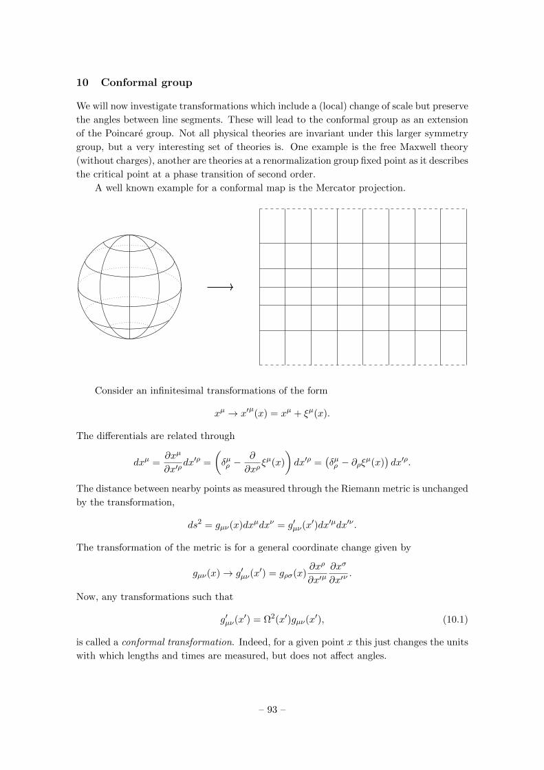
10 Conformal group
We will now investigate transformations which include a (local) change of scale but preserve
the angles between line segments. These will lead to the conformal group as an extension
of the Poincare group. Not all physical theories are invariant under this larger symmetry
group, but a very interesting set of theories is. One example is the free Maxwell theory
(without charges), another are theories at a renormalization group fixed point as it describes
the critical point at a phase transition of second order.
A well known example for a conformal map is the Mercator projection.
Consider an infinitesimal transformations of the form
xµ → x′µ(x) = xµ + ξµ(x).
The differentials are related through
dxµ =∂xµ
∂x′ρdx′ρ =
(δµρ −
∂
∂xρξµ(x)
)dx′ρ =
(δµρ − ∂ρξµ(x)
)dx′ρ.
The distance between nearby points as measured through the Riemann metric is unchanged
by the transformation,
ds2 = gµν(x)dxµdxν = g′µν(x′)dx′µdx′ν .
The transformation of the metric is for a general coordinate change given by
gµν(x)→ g′µν(x′) = gρσ(x)∂xρ
∂x′µ∂xσ
∂x′ν.
Now, any transformations such that
g′µν(x′) = Ω2(x′)gµν(x′), (10.1)
is called a conformal transformation. Indeed, for a given point x this just changes the units
with which lengths and times are measured, but does not affect angles.
– 93 –

Transformations of this type constitute a Lie group, the conformal group. As usual
we will discuss this in terms of the Lie algebra that governs transformations close to the
identity.
For an infinitesimal transformation we expand to linear order,
Ω2(x) = 1 + κ(x), (10.2)
and we use∂xρ
∂x′µ= δρµ − ∂µξρ(x).
Inserting this in (10.1) yields the conformal Killing equation
gµσ∂ρξµ + gρν∂σξ
ν + ξλ∂λgρσ + κgρσ = 0. (10.3)
A solution ξµ(x) is called conformal Killing vector field. It parametrizes a change of
coordinates for which the metric is invariant up to a conformal factor. Solutions with κ = 0
is called a Killing vector field and it parametrises a change of coordinates for which the
metric does not change at all. This is obviously a stronger condition. [Exercise: Show that
the expansion (10.2) together with (10.1) implies the conformal Killing equation (10.3).]
While the above considerations apply in principle to different spacetime geometries, it
is not clear that there are always solutions to the (conformal) Killing equation. Not every
space-time may have useful symmetries.
For many applications, the special case of the Minkowski metric gµν(x) = ηµν is most
interesting. In that case, the conformal Killing equation (10.3) reduces to
∂ρξσ + ∂σξρ + κ ηρσ = 0.
For the case κ = 0 the solutions are at most linear in x,
ξµ(x) = aµ + ωµνxν ,
with antisymmetric ωµν = −ωνµ. These are precisely the Poincare transformations we
discussed in the previous section!
The Poincare group is accordingly a subgroup of the larger conformal group and corre-
sponds to Ω2(x) = 1. As a first example for the more interesting case of κ 6= 0 we consider
the scaling transformation
xµ → λxµ. (10.4)
This is an infinitesimal transformation for λ = 1 + c with infinitesimal c ∈ R. For the
transformation (10.4) the conformal Killing vector and κ are given by
ξµ = cxµ, κ = −2c.
[Exercise: Show this!]
Another example for a conformal transformation is the inversion (we introduce some
arbitrary length l so that units match)
xµ → x′µ(x) =xµ
x2l2. (10.5)
– 94 –

We have
dx′µ = l2δµλx
2 − 2xµxλx4
dxλ,
and thus
ηµνdx′µdx′ν =
l4
x4ηµνdx
µdxν .
This is indeed a conformal transformation! However, such an inversion cannot be continu-
ously deformed to the identity transformation, which means that we need to do more steps
to find the Lie algebra of the conformal group.
Let us therefore consider the chain
xµinversion→ xµ
x2l2
translation→ xµ
x2l2 + bµl2
inversion→xµ
x2+ bµ
ηρσ
(xρ
x2+ bρ
)(xσ
x2+ bσ
)and expand the final result to linear order in b,
xµ → x′µ = xµ + bλ(ηµλx2 − 2xµxλ).
This implies that
ξµ(x) = bλ(ηµλx2 − 2xµxλ),
must be a conformal Killing vector. (One may of course check this directly.) The transfor-
mations
xµ → xµ + bλ(ηµλx2 − 2xµxλ), (10.6)
are also known as infinitesimal versions of special conformal transformations. In addition
to the dilations (10.4), we have in d = 4 dimensions with the transformations (10.6) a
1 + 4 = 5 parameter class of transformations in addition to the already existing 6 + 4 = 10
parameters of the Poincare group. The conformal group is rather large, which makes it
quite powerful in practise.
Let us go back to the conformal Killing equation (10.3). By contracting it with gρσ
one finds in Minkowski space with d the number of spacetime dimensions,
κ = −2
d∂µξ
µ.
Inserting this into the conformal Killing equation and taking another derivative yields
d∂µ∂µξσ = (2− d)∂σ∂µξ
µ.
For d = 2 the equation ∂µ∂µξσ = 0 has infinitely many solutions so that conformal symme-
try is even more powerful. In fact, every holomorphic function induces then a conformal
map if the two coordinates are identified with real and imaginary parts of a complex vari-
able. In contrast, for d > 2, the vector field ξσ can be at most quadratic in xµ,
ξµ = aµ + ωµνxν + cxµ + bλ(ηµλx2 − 2xµxλ).
The analysis given above is complete in this sense.
– 95 –

Let us now find the Lie algebra. This is most easily done by writing the generators in
a specific representation. When acting on fields, the generators of the conformal algebra
areD = −ixµ∂µ,Pµ = −i∂µ,Cµ = −i(δνµx2 − 2xµx
ν)∂ν ,
Mµν = −i(xµ∂ν − xν∂µ).
As we have seen for Lorentz transformations, it may be necessary to add an internal
representation part when generators act on a specific field. For example, the dilation
operator also contains a part that goes with the engineering dimension of a field. We
already know the commutation relations of Pµ and Mµν . We notice that
[iD, (xα1 · · ·xαn)] = n(xα1 · · ·xαn),
[iD, (∂α1 · · · ∂αn)] = −n(∂α1 · · · ∂αn).
This means that iD “measures” in this sense the engineering dimension of an expression.
The remaining non-trivial commutation relations can now be easily worked out and read
[D,Pµ] = iPµ,
[D,Cµ] = −iCµ,[D,Mµν ] = 0,
[Cµ, Cν ] = 0,
[Mµν , Cρ] = i(ηµρCν − ηνρCµ),
[Cµ, Pν ] = −2i(Mµν + ηµνD).
(10.7)
The first two lines tells that Pµ has dimension of momentum and Cµ has dimension of
length, while the third line tells that Mµν is dimensionless and D transforms as a scalar
under Lorentz transformations. The second to last line tells that Cρ transforms appropri-
ately under Lorentz transformations. [Exercise: Derive the commutation relations (10.7).]
One can actually show that the commutation relations of the conformal group in
d = 1 + 3 dimensions correspond to the one of the indefinite orthogonal group in d = 2 + 4
dimensions. In other words, the conformal Lie algebra is actually so(2, 4). [Exercise: Find
this correspondence!]
– 96 –

11 Non-relativistic space-time symmetries
Quantum field theories can also be used in the non-relativistic regime, i. e. at energies that
are much smaller than mc2. As an example, consider the action for a scalar field
S =
∫dtdd−1x
ϕ∗(t, ~x)
[i∂t +
~∇2
2m− V (t, ~x)
]ϕ(t, ~x)− λ
2ϕ∗2(t, ~x)ϕ2(t, ~x)
. (11.1)
We include here an external potential V (t, ~x) that couples to the density ϕ∗ϕ and a two-
particle contact interaction strength λ. The action is written in one time and d− 1 space
dimensions. On a classical level, variation of (11.1) leads to the Gross-Pitaevskii equation.
What are the symmetries? Formally one could study the non-relativistic limit of the
Poincare algebra, but it is more transparent to establish the symmetries directly in the
non-relativistic regime.
11.1 Symmetries of non-relativistic quantum field theories
Galilei group. As a low energy limit of the Poincare group, we have in the non-
relativistic regime the following space-time transformations
(t, xj)→ (t+ a,Rj kxk + vjt+ bj). (11.2)
This includes translations in time by an amount a, translations in space by ~b, rotations in
space through the matrix R and Galilei boosts with the velocity ~v. A Galilei transformation
consists of several elements (R, a,~v,~b), with the composition law
(R2, a2, ~v2,~b2) (R1, a1, ~v1,~b1) = (R2R1, a2 + a1, ~v2 +R2~v1,~b2 +R2~b1 + ~v2a1).
While the composition law looks a bit involved, it is clear that such Galilei transformations
form a group, the Galilei group. In the following we study how the different elements are
implemented as transformations of non-relativistic quantum fields.
Rotations. Rotations are realized as in the relativistic case with hermitian generators
Jj = 12εjklMkl. When acting on a scalar field we have Mkl =Mkl where
Mkl = −i(xk∂l − xl∂k).
The action on a scalar field is simply
ϕ(t, ~x)→ ϕ′(t, ~x) = ϕ(t, R−1~x).
For non-relativistic spinor or tensor fields, this is supplemented by the appropriate gener-
ator acting on the “internal” representation of the field.
– 97 –

Translations in space and time. Translations in space and time are also implemented
as in the relativistic case. They are generated by
P0 = −H = −i ∂∂t, Pj = −i ∂
∂xj.
The action of a finite group element on the scalar field is
ϕ(t, ~x)→ ϕ′(t, ~x) = ϕ(t− a, ~x−~b).
For an infinitesimal transformation this becomes
ϕ(t, ~x)→ ϕ′(t, ~x) =(1− idaP0 − idbjPj
)ϕ(t, ~x).
The last equation is for an infinitesimal transformation. Eigenfunctions are plane waves,
e−iωt+i~p~x, as usual.
Galilei boosts. Galilei boosts are realized in a somewhat non-trivial way. The scalar
field transforms as
ϕ(t, ~x)→ ϕ′(t, ~x) = eim~v~x−im~v2t
2 ϕ(t, ~x− ~vt). (11.3)
The non-trivial point is here the appearance of an additional phase factor which involves
the boost velocity ~v. Expanding this to linear order in dvj , we find that an infinitesimal
transformation can be written as
ϕ(t, ~x)→ ϕ′(t, ~x) =(1− idvjKj
)ϕ(t, ~x),
where the boost generator is
Kj = −mxj − it∂
∂xj.
In particular, we see that this depends through the first term on the particle mass m. We
also make the observation that in contract to the generator of a Lorentz transformation,
the generator of a Galilei boost is hermitian, Kj = K†j . Indeed, the Galilei group can
be made compact when time and space are compactified, such as with periodic boundary
conditions.
Lie algebra. We can now state the commutation relations. We have
[Pj , Pk] = [P0, Pk] = [Kj ,Kk] = 0,
[Jj , Jk] = iεjklJl,
[Jj , P0] = 0
[Jj , Pk] = iεjklPl, [Jj ,Kk] = iεjklKl,
[Kj , P0] = −iPj ,[Kj , Pk] = −imδjk.
(11.4)
Particularly interesting is the last line. It tells that the Lie algebra has been extended
by a so-called central charge, given here by the particle mass m. Note that such a mass
was not present when we first specified Galilei transformations in (11.2). As they stand,
– 98 –

the commutation relations (11.4) form a central extension of the Galilei algebra. There
are many different such central extensions of the algebra; in particular the mass m is not
constrained, except for being real and positive. There are also representations of the Galilei
algebra on fields that do not need such a central extension, for example in non-relativistic
fluid dynamics.
Related to the central charge is the appearance of the U(1) phase factor in (11.3). One
says that this is a projective representation; in some sense a representation of the Galilei
group without central extension up to a phase. This comes with a superselection rule:
linear superpositions of states with different mass are not allowed. Alternatively one may
introduce one more element of the Lie algebra, a mass operator M which has eigenvalue
m for a specific representation of a field for a particle with mass m. In that case, the last
line in (11.4) is replaced by
[Kj , Pk] = −iMδjk,
[M,P0] = [M,Pj ] = [M,Jj ] = [M,Kj ] = 0.
With this prescription we have again an ordinary representation (instead of a projective
one), but now in a larger algebra. The mass operator commutes with all other operators,
that is why one says that it is in the center of the algebra.
Galilei covariant derivative. It is instructive to work out how different elements in the
action (11.1) transform under Galilei boost transformations. First of all, the interaction
term is covariant,
λ
2ϕ∗2(t, ~x)ϕ2(t, ~x)→ λ
2ϕ∗2(t, ~x− ~vt)ϕ2(t, ~x− ~vt).
The phase factors in (11.3) cancel out and the net effect is just the one of a translation in
space by and amount ~vt. Now consider the time derivative term,
ϕ∗(t, ~x) [i∂t]ϕ(t, ~x)→ ϕ∗(t, ~x− ~vt)[i∂t +
m~v2
2− i~v ~∇
]ϕ(t, ~x− ~vt).
This is not covariant! Let us also consider the spatial derivative term
ϕ∗(t, ~x)
[~∇2
2m
]ϕ(t, ~x)→ ϕ∗(t, ~x− ~vt)
[~∇2
2m− m~v2
2+ i~v ~∇
]ϕ(t, ~x− ~vt).
We observe that neither the time derivative term nor the spatial derivative terms are Galilei
covariant by themselves. However, their combination is. One may state this by saying that
the combination
D = i∂t +~∇2
2m, (11.5)
is acting as a covariant derivative with respect to Galilei boost transformations. In fact,
for this combined derivative operator one has the Galilei boost transformation
Dϕ(t, ~x)→ Deim~v~x−im~v2t
2 ϕ(t, ~x− ~vt) = eim~v~x−im~v2t
2 Dϕ(t, ~x− ~vt).
The covariant derivative of a scalar field Dϕ transforms just as the field ϕ itself. Any
power of D also has this property, this is important to construct invariant terms that can
appear in a quantum effective action.
– 99 –
Global U(1) transformations. The action (11.1) has another symmetry, namely under
global U(1) transformations,
ϕ(t, ~x)→ eiαϕ(t, ~x), ϕ∗(t, ~x)→ e−iαϕ∗(t, ~x).
This is rather easy to check. The physical consequence of this symmetry is the conservation
law for particle number which can be stated in local form as
∂tn+ ~∇~n = 0.
Here n = ϕ∗ϕ is the particle number density and
~n = − i
m
(ϕ∗~∇ϕ− ϕ~∇ϕ∗
),
is the corresponding current.
Time-dependent U(1) transformations. There is also a way to make the U(1) trans-
formations time dependent,
ϕ(t, ~x)→ eiα(t)ϕ(t, ~x), ϕ∗(t, ~x)→ e−iα(t)ϕ∗(t, ~x).
One would say that this is in conflict with the time derivative term which transforms as
[i∂t]ϕ→ [i∂t] eiα(t)ϕ = eiα(t) [−∂tα(t) + i∂t]ϕ.
However, this change can be compensated by a change in the external potential,
V (t, ~x)→ V (t, ~x)− ∂tα(t).
In other words, the combination
i∂t − V (t, ~x),
acts as a covariant derivative with respect to time-dependent U(1) transformations! The
extended combination
D = i∂t +~∇2
2m− V (t, ~x),
is now a covariant derivative for both Galilei boost and time-dependent U(1) transforma-
tions.
As a special case of a time-dependent U(1) transformation consider
ϕ(t, ~x)→ e−i∆V tϕ(t, ~x), V (t, ~x)→ V (t, ~x) + ∆V.
This changes the field ϕ by an oscillating phase and the external potential by an additive
constant. For a massive relativistic scalar field, the solutions to the equations of motion
have oscillations with frequency proportional to the rest mass, actually mc2. In the non-
relativistic limit we have taken mc2 →∞ and the above symmetry is a direct consequence
of this limit. In the non-relativistic quantum mechanical formalism this corresponds to the
observation that the absolute scale of potential energy can be chosen at will.
– 100 –

11.2 Scaling transformations in the non-relativistic regime
The question comes up what happens to conformal transformations in the non-relativistic
regime. There is in fact an algebra known as the conformal Galilean algebra that contains
analogously to the relativistic conformal group also 15 generators. However, this is not the
invariance group of the free Schrodinger equation. In fact, for the non-relativistic limit of a
relativistic quantum field theory, the particle mass m is crucial. It is intuitively clear that
this leads to a partial breaking of relativistic conformal invariance, because this is only a
symmetry for theories with massless particles (or no quasi-particles at all).
Despite this, there is also a non-relativistic version of scaling symmetry and the sym-
metry group of the free Schrodinger equation, the so-called Schrodinger group has a Lie
algebra that contains in addition to Galilei algebra (with central extension) in (11.4) two
more generators.
Dilatations. To find the non-relativistic version of a dilatation let us first note that the
operator in (11.5) contains a quadratic space and a linear time derivative. It is therefore
not consistent to rescale time and space coordinates by the same factor but rather one
should do the rescaling according to
(t, ~x)→(λ2t, λ~x
). (11.6)
In this sense, time counts in the non-relativistic domain as having dimension of length
squared! (More precisely this works in units where mass m is effectively dimensionless.)
In the following we also need to know the scaling dimension of a scalar field as it
appears in the action (11.1). The action S itself must be dimensionless. The combination
dtdd−1x has with the counting we just established dimension of length to the power d+ 1.
The time derivative term has length dimension (−2) and accordingly the field ϕ must have
dimension of length to the power (1−d)/2, where d−1 is the number of spatial dimensions.
We can now state the action of a dilation transformation acting on the field,
ϕ(t, ~x)→ ϕ′(t, ~x) = λ(1−d)/2ϕ(λ−2t, λ−1~x).
For an infinitesimal transformation λ = 1 + c this can be written as
ϕ(t, ~x)→ ϕ′(t, ~x) = (1− icD)ϕ(t, ~x),
with the dilatation operator acting acting on the scalar fields given by
D = −i(xj
∂
∂xj+ 2t
∂
∂t
)− id− 1
2.
This is such that iD measures the non-relativistic scaling dimensions of an expression, for
example [iD, xj ] = xj , [iD, ∂j ] = −∂j , [iD, t] = 2t and [iD, ∂t] = −2∂t.
We can immediately state the commutation relation with the generators of the Galilei
algebra. They are given by
[D,Jj ] = 0, [D,Pj ] = iPj , [D,P0] = 2iP0,
[D,Kj ] = −iKj , [D,M ] = 0.(11.7)
– 101 –

Note again that mass is effectively dimensionless in the units measured by D. For vanishing
external potential V (t, ~x) = 0, and vanishing interaction strength λ = 0, the action (11.1)
contains no dimensionfull external parameter and is then invariant under the dilatations
generated by D.
Scaling symmetry in two dimensions. One may also work out the scaling dimension
of the interaction λ and finds that it has dimension of length to the power d − 3. In
particular for d− 1 = 2 spatial dimensions one finds that λ is dimensionless. On a classical
level there is then accordingly a scaling symmetry also for the interacting system. However,
this scaling symmetry is broken by quantum fluctuations. More specifically, the interaction
parameter λ becomes scale dependent as a consequence of the renormalization group flow.
Time-dependent scaling or “Schrodinger expansion”. There is another interesting
symmetry of the free Schrodinger equation, namely it is invariant with respect to the time-
dependent scaling
(t, ~x)→ (t′, ~x′) =
(t
1 + ft,
~x
1 + ft
). (11.8)
Here we are using a real parameter f with dimension of inverse time. As an infinitesimal
transformation this reads
(t, ~x)→ (t′, ~x′) = (t− dft2, ~x− dft~x).
To see that the scaling (11.8) is indeed a symmetry requires a few calculations. We con-
centrate on the infinitesimal transformation where one has
dt = (1 + 2dft)dt′, dxj = (1 + dft)dx′j ,
such that we can replace in the action (11.8)
dtdd−1x→ [1 + (d+ 1)dft] dt′dd−1x′.
To transform also the other terms we need to study how partial derivatives are related.
For the spatial derivative this is straight-forward,
∂
∂xj=
∂t′
∂xj∂
∂t′+∂x′k
∂xj∂
∂x′k= (1− dft) ∂
∂x′j,
so there is just a time-dependent scaling. For the time derivative there is an extra term,
∂
∂t=∂t′
∂t
∂
∂t′+∂x′k
∂t
∂
∂x′k= (1− 2dft)
∂
∂t′− dfxj ∂
∂x′j.
Without this extra term one could establish a symmetry of the action (11.8) by just rescal-
ing also the fields in an appropriate way. Now we need also an additional position dependent
phase factor. Accordingly, the infinitesimal transformation of the fields is
ϕ(t, ~x)→ ϕ′(t, ~x) = (1− idfC)ϕ(t, ~x),
with the generator for a special conformal transformation in the representation ϕ
C = −i(t2∂
∂t+ txj
∂
∂xj
)− itd− 1
2− 1
2m~x2. (11.9)
– 102 –

Full Schrodinger algebra. We can now state the full Lie algebra of symmetries for the
free Schrodinger equation. The Galilei algebra with central extension (11.4) is extended
by the operators for non-relativistic dilations D with the commutation relations (11.7).
In addition to this, there are special conformal transformations C with the additional
commutation relations
[C, Jj ] = 0, [C,Kj ] = 0, [C,Pj ] = iKj ,
[C,P0] = iD, [C,D] = 2iC.(11.10)
This closes the algebra. Not counting the central generator for mass M we have 12 gen-
erators. Let us emphasize again that the full Schrodinger group can only be applied in
exceptional cases such as the free Schrodinger equation or at a renormalization group fixed
point of an interacting system.
The subgroup of Galilei transformations is more useful and applies quite generally to
few-body systems in the non-relativistic regime. It can also be broken, however, as in
a state of condensed matter. As an example, the fluid rest frame singles out a specific
frame and therefore breaks Galilei boost symmetry. Also translation invariance and rota-
tion symmetry can be broken in various ways, for example through the external potential
V (t, ~x).
[Exercise: Investigate the subgroup of the Schrodinger group formed by translations in
time, dilatations, and special conformal transformations. Find the infinitesimal and finite
group transformations and establish a correspondence to SL(2,R).]
– 103 –

12 Consequences of symmetries for effective actions
Now that we have discussed many different symmetries that appear in different physics
problems, specifically in the context of quantum theory, let us pause for a moment and
discuss what consequences follow from this. We will perform this discussion in the context
of quantum field theory after analytic continuation from a space with Minkowski signature
of the metric to a Euclidean signature.
12.1 Functional integral, partition function and effective action
We consider a theory for quantum fields χ(x) which we do not specify in further detail
here. In practise χ(x) stands typically for a collection of different fields and may encompass
components transforming as scalars, vectors, tensors, or spinors. The theory is described
by a microscopic action S[χ]. The latter enters the partition function
Z[J ] =
∫Dχ e−S[χ]+
∫x J(x)χ(x). (12.1)
We use here the functional integral∫Dχ. We cannot go here into the details of its con-
struction and refer to a lecture course on quantum field theory. From the partition function
one defines the Schwinger functional W [J ] = lnZ[J ] and from there the quantum effective
action or one-particle irreducible effective action Γ as a Legendre transform,
Γ[φ] = supJ
(∫xJ(x)φ(x)−W [J ]
). (12.2)
The effective action Γ[φ] depends on φ, which is the expectation value of the field χ. To
see this one evaluates the supremum by varying the source field J(x) leading to
φ(x) =δ
δJ(x)W [J ] =
1
Z[J ]
δ
δJ(x)Z[J ] =
∫Dχ χ(x) e−S[χ]+
∫Jχ∫
Dχ e−S[χ]+∫Jχ
.
One also writes this as
φ(x) = 〈χ(x)〉,
with the obvious definition of the expectation value 〈·〉 in the presence of sources J . An
interesting property of Γ[φ] is its equation of motion. It follows from the variation of (12.2)
asδ
δφ(x)Γ[φ] = J(x). (12.3)
In particular, for vanishing source J = 0, one obtains an equation that resembles very
much the classical equation of motion, δS/δχ = 0. However, in contrast to the latter,
(12.3) contains all corrections from quantum fluctuations! Another interesting property is
that tree-level Feynman diagrams become formally exact when propagators and vertices
are taken from the effective action Γ[φ] instead of the microscopic action S[χ].
– 104 –

12.2 Symmetry transformations of microscopic action
Both the microscopic action S[χ] and the quantum effective action Γ[φ] are functionals of
fields. When one speaks of a symmetry transformation of the action one means in practise
a symmetry transformation of the fields on which the action depends. A symmetry of the
microscopic action means an identity of the form
S[gχ] = S[χ].
Here the group element g ∈ G is acting on the fields (not necessarily linearly) and the
symmetry implies that the action is unmodified by this transformation. So far, G could be
either a finite group, an infinite discrete group or a continuous Lie group. In the latter case
one can decompose finite group transformations into infinitesimal transformations. One
can write
S[gχ] = S[(1+ idξjTj
)χ]
= S[χ] +
∫x
δS[χ]
δχ(x)idξj(Tjχ)(x).
One also abbreviates this as S[χ] + dS[χ] and a continuous symmetry corresponds then to
the statement dS[χ] = 0. This needs in particular the infinitesimal change in the field
χ(x)→ χ′(x) = χ(x) + dχ(x) = χ(x) + idξj(Tjχ)(x), (12.4)
where Tj is an appropriate representation of the Lie algebra acting on the fields (not
necessarily linearly).
12.3 Symmetry transformation of integral measure
The functional integral measure can also be transformed. One says that it is invariant if
Dχ = D(gχ).
An example for this would be a generalization of a change of integration variable xj →f j(~x), where one would in general expect a Jacobian determinant, dNx = |det(∂xj/∂fk)|dNf(x).
The above equation tells that this determinant is unity. (More generally one may also allow
a field independent constant that can be dropped for many purposes.) Again this goes for
elements g ∈ G of finite, discrete or continuous groups G.
It can happen that one finds a symmetry of a microscopic action S[χ] but that the
functional integral measure is not invariant. In that case one speaks of a quantum anomaly.
12.4 Continuous symmetries of effective actions
We now specialize to continuous transformations which we can study in infinitesimal form
(12.4). After a change of integration variable χ → gχ we write the Schwinger functional
(12.1) as
Z[J ] =
∫D(χ+ idξjTjχ
)e−S[χ+idξjTjχ]+
∫x J(x)(χ(x)+idξjTjχ(x)).
– 105 –

We now assume the invariance of the measure D(χ+ idξjTjχ
)= Dχ, or, in other words,
the absence of an anomaly. This leads for small dξj to
Z[J ] =
∫Dχ e−S[χ+idξjTjχ]+
∫x J(x)(χ(x)+idξjTjχ(x))
=
∫Dχ
[1 +
∫x
(− δ
δχ(x)S[χ] + J(x)
)idξjTjχ(x)
]e−S[χ]+
∫x J(x)χ(x).
The leading term on the right hand side is just Z[J ] itself. Subtracting it we find using
(12.3) the Slavnov-Taylor identity
〈dS[χ]〉 =
⟨∫x
(δ
δχ(x)S[χ]
)idξjTjχ(x)
⟩=
∫x
(δ
δφ(x)Γ[φ]
)idξj 〈Tjχ(x)〉 . (12.5)
An important class of transformations is such that the Lie algebra generators Tj act on the
fields χ in a linear way. In that case one can write
〈Tjχ(x)〉 = Tj 〈χ(x)〉 = Tjφ.
In that case the right hand side of (12.5) can be written as dΓ[φ] and one has
〈dS[χ]〉 = dΓ[φ]. (12.6)
In particular, the most important case is here that the microscopic action is invariant,
dS[χ] = 0, from which it follows that also the effective action is invariant, dΓ[φ] = 0, or
Γ[gφ] = Γ[φ].
In summary, in the absence of a quantum anomaly, and for a linear representation of the
Lie algebra on the fields, we conclude that the effective action Γ[φ] shares the symmetries
of the microscopic action S[χ]. This is very useful in practice because it constrains very
much the form the effective action can have. This is important for example for proofs of
renormalizability or also for solving renormalization group equations in practice.xx
Extended symmetries. Interestingly, eq. (12.6) is also useful when the microscopic
action S[χ] is not fully invariant, i. e. dS[χ] 6= 0. Specifically, if dS[χ] is linear in the field
χ, one can infer that the effective action Γ[φ] must change in the same way such that (12.6)
remains fulfilled. This can also constrain the form of Γ[φ] substantially. All this assumes
invariance of the functional integral measure, though.
One can also often make use out of anomalous symmetries, i. e. symmetry trans-
formations where the functional measure is not invariant, if the corresponding Jacobian
determinant can be absorbed into a change of the action.
12.5 Conservation laws for field theories
We have already briefly discussed the close relation between continuous symmetries and
conservation laws in terms of Noethers theorem earlier. Here we will briefly discuss how this
extends to classical field theories as described by the action S[χ]. An extension to quantum
field theories and a description in terms of the effective action Γ[φ] will be discussed later.
– 106 –

Assume that we have an action S[χ] that is invariant under a global transformation of
the fields
χ(x)→ χ(x) + idξjTj(x).
Here the adjective global refers to dξj being independent of position x. By the statement
that S[χ] is invariant we mean dS = 0. More generally, one may allow the change of S[χ]
by a boundary term, such that one can write dS for a global transformation as an integral
over a total divergence,
dS = iξj∫x∂µFµj (x).
Because such boundary terms do not contribute to the equations of motion one can drop
them for many purposes and we will do so below.
As a calculational trick we allow now the transformation become local, dξj → dξj(x).
We can then write up to boundary terms
dS = i
∫x
J µj (x)∂µdξ
j(x) +Kµνj (x)∂µ∂νdξj(x) + . . .
Because we have assumed a global symmetry, the derivative expansion on the right hand
side starts with the terms proportional to the first derivative ∂µdξj . The objects J µj (x)
and Kµνj (x) depend on the field χ which is evaluated at the solution to the classical field
equation δS/δχ = 0. In principle, higher orders in derivatives may appear, but typically,
for microscopic actions S[χ] this is not the case and already Kµν(x) often vanishes.
Let us now perform a partial integration. Dropping again boundary terms we find
dS = i
∫x
[−∂µJ µj (x) + ∂µ∂νKµνj (x)− . . .
]dξj(x)
.
Because dξj(x) is arbitrary and for stationary action dS = 0, we find one local conservation
law for each Lie algebra generator Tj ,
∂µJµj (x) = 0,
where
Jµj (x) = J µj (x)− ∂νKµνj (x) + . . . .
In principle this derivation would extend also to the quantum effective action Γ[φ]
and should then give a conservation law for currents where quantum effects have been
taken into account. However, in that case it is less clear that the expansion in powers
of derivatives terminates, and the construction is therefore not as useful. A possibility
to solve this problem is to extend the global symmetry to a local symmetry in a more
sophisticated way, namely by introducing (external) gauge fields. This will be discussed in
a later section.
– 107 –

13 Non-Abelian gauge theories
A gauge theory has a local symmetry as opposed to a global symmetry. Let us discuss this
immediately for a non-abelian group, such as SU(N) (recall our discussion of matrix Lie
groups in section 6.3). For some matter field ψa(x) in the fundamental representation the
local transformation reads
ψa(x)→ Uab(x)ψb(x) = exp[iξj(x)Tj ]ab ψ
b(x) (13.1)
where Uab(x) depends now through the parameter fields ξj(x) on space and time. In order
to construct theories involving such local symmetries one needs a covariant derivative such
that with the field transforming like (13.1) its covariant derivative transforms similarly,
(Dµ(x))abψb(x)→ Uab(x)(Dµ(x))bcψ
c(x). (13.2)
The covariant derivative is written as
(Dµ(x))ab = ∂µδab − i(Aµ(x))ab = ∂µδ
ab − iAjµ(x)(Tj)
ab.
We use in the first equation a notation where the gauge field (Aµ(x))ab is a field which for
every space-time position x and index µ is an element of the Lie algebra, i. e. it is matrix
valued. One may decompose this further in terms of a set of generators of the Lie algebra
Tj in the fundamental representation,
(Aµ(x))ab = Ajµ(x)(Tj)ab, (13.3)
so that Ajµ(x) is the corresponding coefficient field.
Under the local transformation (13.1), the gauge field transforms as
(Aµ(x))ab → Uac(x)(Aµ(x))cd(U−1)db(x)− iUac(x)∂µ(U−1)cb(x). (13.4)
Indeed this makes sure that (schematically) Dµ(x)→ U(x)Dµ(x)U−1(x), such that (13.2)
is indeed fulfilled. Note that the first term in the transformation (13.4) is such that it is
corresponds to the standard transformation law for a field with one upper and one lower
index. (This is essentially how matter fields transform.) More precisely, we recognize here
the adjoint representation of the gauge group. However, the second term spoils this and is
characteristic for a gauge field. [Exercise: Consider two fields (Aµ(x))ab and (Bµ(x))ab that
transform both as gauge fields. Show that the difference (Aµ(x))ab− (Bµ(x))ab transforms
as an ordinary matter field.]
One may also define the field strength tensor (also a Lie algebra valued field; we drop
the indices a, b, . . . for simplicity)
Fµν(x) = i[Dµ(x), Dν(x)] = ∂µAν(x)− ∂νAµ(x)− i[Aµ(x), Aν(x)].
Under gauge transformations this transforms covariantly (as a matter field in the adjoint
representation of the gauge group),
Fµν(x)→ U(x)Fµν(x)U−1(x).
– 108 –

Similar to (13.3) one can also write the field strength tensor as
(Fµν(x))ab = F jµν(x)(Tj)ab,
and using the structure constants
[Tj , Tk] = if ljk Tl,
one finds then
F jµν(x) = ∂µAjν(x)− ∂νAjµ(x) + f j
mn Amµ (x)Anν (x).
Finally, let us write down a kinetic term for gauge fields, as it appears in the La-
grangian. The construction principle is the action should be invariant. An allowed term
involving only the gauge field is
S =
∫ddx
− 1
2g2trFµν(x)Fµν(x)
=
∫ddx
− 1
2g2(Fµν(x))ab(F
µν(x))ba
.
It is immediately clear that this is gauge invariant. One may also write this in terms of
generators Tj . In that case the action becomes
S =
∫ddx
−cRδjk2g2
F jµν(x)F kµν(x)
.
We assumed here that the generators are normalized according to
TrTjTk = cRδjk,
with a constant cR that depends on the representation R. For su(2) and su(3) we had
chosen generators such that in the fundamental representation cR = 1/2 and that can
be done more generally for su(N). In fact one can relate cR to the dimension dR of the
representation R (such that the generators Tj are in this representation dR×dR matrices),
the dimension dA of the adjoint representation (equal to the number of generators), and
the eigenvalue of the quadratic Casimir operator in the representation R defined by
C2 = TjTj = cR2 1.
The relation is [Exercise: Show this!]
cR =dRc
R2
dA.
13.1 Gauge group of the standard model
The gauge group of the standard model of elementary particle physics is
SU(3)⊗ SU(2)⊗U(1).
– 109 –

The fermion fields and the Higgs boson scalar field can be classified into representations of
the corresponding Lie algebras. With respect to the strong interaction group SU(3)colour
we need the representationssinglet 1,
triplet 3,
anti-triplet 3∗.
With respect to the weak interaction group SU(2) we need
singlets 1,
doublets 2.
Recall that SU(2) is pseudo-real so there is no independent 2∗. Finally with respect to the
hypercharge group U(1)Y we will classify fields by their charge as generalisations of electric
charge q. The charges turn out to be
0 , ±1
6, ±1
3, ±1
2,
2
3, ±1 .
Moreover the fermions transform as Weyl spinors under the Lorentz group, either left- or
right-handed. There are the following fields(νLeL
)neutrino
electronleft-handed
(1, 2, −1
2
)(νL eL
) anti-neutrino
anti-electronright-handed
(1, 2,
1
2
)eR electron right-handed
(1, 1, −1
)eR anti-electron left-handed
(1, 1, 1
)(uLdL
)up-quark
down-quarkleft-handed
(3, 2,
1
6
)(uL dL
) anti-up-quark
anti-down-quarkright-handed
(3∗, 2, −1
6
)uR up-quark right-handed
(3, 1,
2
3
)uR anti-up-quark left-handed
(3∗, 1, −2
3
)dR down-quark right-handed
(3, 1, −1
3
)dR anti-down-quark left-handed
(3∗, 1,
1
3
)φ Higgs-doublet scalar
(1, 2,
1
2
)
– 110 –

where the last expression determines the representations under the gauge symmetries. The
fields have several indices corresponding to the different groups, for example(uR)am
where a ∈ 1, 2 is the Lorentz spinor index and m ∈ 1, 2, 3 is the SU(3)colour index.
The leptons and quarks come in three copies, also known as families. For example, in
addition to the electrons and anti-electrons there are also muons and tau leptons with their
corresponding anti-particles and an associated neutrino. For the quarks we have discussed
this already.
In addition to these “matter fields”, there are corresponding gauge bosons, specifically
for SU(3)color the eight real gluons, for SU(2) three real gauge bosons and one for the
abelian U(1)Y subgroup. After spontaneous symmetry breaking, the SU(2)⊗U(1)Y bosons
combine into the two massive complex W± bosons, the neutral and massive Z boson and
the massless photon. The symmetry breaking itself is due to an expectation value for the
scalar Higgs field.
– 111 –

14 Grand unification
14.1 SU(5) unification
We now discuss a proposed extension of the Standard Model which leads to a unification
of the gauge groups into SU(5). This has been proposed by Howard Georgi and Sheldon
Glashow in 1974.
Note that the SU(3) and SU(2) generators naturally fit into SU(5) generators and
similar for the spinors (
3× 3
)SU(3) (
2× 2
)SU(2)
ψ1
ψ2
ψ3
ψ4
ψ5
.
There are 52 − 1 = 24 generators of SU(5) corresponding to the hermitian traceless 5 × 5
matrices. Out of them, eight generate SU(3), while three generate SU(2).
Moreover, within SU(5) there is one hermitian traceless matrix
1
2Y =
−1
3
−13
−13
12
12
.
That generates a U(1) subgroup which actually gives U(1)Y . The remaining generators
correspond to additional gauge bosons not present in the Standard Model so they are
supposedly very heavy or confined. We find the embedding
SU(5)→ SU(3)⊗ SU(2)⊗U(1).
Fundamental representation 5. Now let us consider representations. Take the funda-
mental representation of SU(5) the spinor ψm. From the above illustration one sees that
it decomposes like
5 =
(3, 1, −1
3
)⊕(
1, 2,1
2
),
in a natural way. The conjugate decomposes
5∗ =
(3∗, 1,
1
3
)⊕(
1, 2, −1
2
).
Indeed these could be the representations for the right-handed down quark and the anti-
lepton doublet,
dR,(νL eL
),
and their anti-particles
dR,
(νLeL
),
– 112 –

respectively.
Note that the hypercharges indeed conspire to be such that the generator 12Y is indeed
traceless. It can therefore be one of the generators of SU(5).
Antisymmetric tensor representation 10. So what about the other representations?
The next smallest representation is the anti-symmetric tensor ψmn with dimension ten.
We still need (3, 2,
1
6
),
(3∗, 1, −2
3
),
(1, 1, 1
),
and the corresponding anti-fields. These are ten fields indeed. Now ψmn decomposes into
irreducible representations according to(3, 1, −1
3
)⊗A
(3, 1, −1
3
)=
(3∗, 1, −2
3
),(
3, 1, −1
3
)⊗A
(1, 2,
1
2
)=
(3, 2,
1
6
),(
1, 2,1
2
)⊗A
(1, 2,
1
2
)=
(1, 1, 1
).
This matches indeed to uR, the left-handed quark doublet (uL, dL) and eR, respectively.
Note that we have used here tensor product decomposition relations discussed before
such as for SU(3)
3⊗ 3 = 3∗A ⊕ 6S ,
or for SU(2)
2⊗ 2 = 1A ⊕ 3S .
The U(1) charges are simply added. Indeed things work out! Also in this sector one finds
that the hypercharges add up to zero, 3× 1× (−23) + 3× 2× 1
6 + 1× 1× 1 = 0.
All fermions. The fermion fields of a single generation in the Standard Model can be
organised into the SU(5) representations
5∗ : dR,
(νLeL
),
and
10 : uR, eR,
(uLdL
),
as well as the corresponding anti-fields. There is no space here for a right handed neutrino,
it would have to be a singlet 1 under SU(5).
The scalar Higgs field could be part of a 5 scalar representation but the corresponding
field with quantum numbers (3, 1, −2
3
)is not present in the Standard Model and must be very heavy or otherwise suppressed.
– 113 –

Gauge bosons. The gauge bosons of SU(5) can be found from decomposing 5 ⊗ 5∗ =
24 + 1. In terms of SU(3)⊗ SU(2)⊗U(1) the 24 decomposes into
24 =
(1, 3, 0
)⊕(
8, 1, 0
)⊕(
1, 1, 0
)⊕(
3, 2,2
3
)⊕(
3∗, 2, −2
3
).
We recognize the W boson triplet, the gluons, the hypercharge photon and two more gauge
bosons that transform under both SU(3)color and the electroweak group SU(2)×U(1). The
latter type of gauge bosons could in principle induce transitions of the type
d→ e+,
u→ u,
and thus u+ d→ u+ e+ causing
uud→ uu+ e+,
p→ π0 + e+.
The proton could therefore decay! This is actually one of the main experimental signatures
for such grand unified theories.
Proton decay has not been observed so the transition rate must be very small. This
also implies that the unification scale where the three forces SU(3)color, SU(2) and U(1)Yunite, must be very high. The latest experimental constraint is that the proton half-life
time must be at least 1.6× 1034 years [Super-Kamiokande, PRD 95, 012004 (2017)]. If the
decay rate goes like
Γ ≈m5p
M4GUT
,
one can estimate for the unification scale MGUT > 1016 GeV.
The Georgi-Glashow model we discussed so far is not very realistic, in some sense
it is already ruled out. For example it predicts massless neutrinos, which is in conflict
with the observation of neutrino oscillations. Also the unification of renormalization group
trajectories to a single SU(5) coupling constant at the scale MGUT does not seem to work
as it should.
Charge quantization. Besides the nice matching of the representations, there is another
theoretical reason that speaks for a unified gauge theory. In the standard model it is not
explained by electric charge to be a multiple of the electron charge (with fractional charges
1/3 for the quarks). In the SU(5) model the U(1)Y generator is part of SU(5) and it is
naturally explained why the charges have the values they have.
14.2 SO(10) unification
There are further possibilities to construct unified theories. The Pati-Salam model for
example has the gauge group SU(4)× SU(2)L × SU(2)R.
Both the Georgi-Glashow and the Pati-Salam model can be further unified and em-
bedded into the group SO(10). The unified gauge theory based on SO(10) is particularly
– 114 –

elegant, but we will not discuss it in detail here. Let us just mention that there is a
spinorial representation (similar to the left-handed or right-handed spinor representations
of SO(1, 3) for chiral fermions) 16, that decomposes in terms of SU(5) representations as
16 = 10⊕ 5∗ ⊕ 1.
This contains all the representations we need for the Georgi-Glashow model and therefore
the standard model fermions of one generation as well as one additional fermion that has
the quantum numbers of the right-handed neutrino! The latter is anyway needed for the
seesaw mechanism to give mass to the observable neutrinos. For this mechanism to work,
the right-handed neutrino is supposed to be very heavy. On the other side, in the SO(10)
model, it is part of the 16 representation together with all the other fermions, so it is
supposed to be massless. There must be some mechanism that breaks SO(10) at some high
energy or mass scale and this mechanism needs to give the right-handed neutrino its mass.
One can infer that the scale of SO(10) breaking shows up (albeit somewhat indirectly)
through the seesaw mechanism in the observable neutrino masses and more directly in the
right-handed neutrino mass, which is also a candidate for dark matter.
– 115 –

15 General coordinate and local Lorentz transformations
We started these lectures by stating that symmetries are closely related to conservation
laws. In particular, the translational symmetries of the Poincare group are responsible for
energy and momentum conservation. However, when gravity is taken into account, space-
time becomes curved, and Minkowski space is only a local approximation to it. One may
then ask what happens to the conservation laws and also to concepts like spin or helicity
that seem to be bounded to the symmetries of Minkowski space. To answer these questions,
we will now extend our considerations to general coordinates on some quite general space-
time manifold. The latter may be different from Minkowski space and may also be curved
as is the case in general relativity as a consequence of gravitation. We will discuss here the
tetrad formalism which allows to describe also fermionic in such a situation. The basic idea
of the tetrad formalism is that one the one hand we use a general system of (non-cartesian)
coordinates xµ, but that on the other hand even a curved manifold is locally flat. Moreover,
one can locally choose a frame such that different directions are orthogonal. The tetrad
field will mediate between these two points of view and it will also allow to make Lorentz
transformations local.
The present section assumes some familiarity with standard concepts of differential
geometry as they are taught for example in a course on general relativity.
15.1 Tetrad formalism
The tetrad field can be defined through a local choice of an orthogonal frame, or formally
as a Lorentz vector valued one-form V Aµ (x)dxµ. The latin index A is here a Lorentz index
(in a sense to be made more precise below), while the Greek index µ is a general coordinate
index. With Minkowski metric ηAB = diag(−1,+1,+1,+1) one can write the Riemannian
coordinate metric gµν(x) as
gµν(x) = ηABVAµ (x)V B
ν (x). (15.1)
We also introduce the inverse tetrad V µA(x) such that
V Aµ (x)V ν
A(x) = δ νµ , V A
µ (x)V µB(x) = δAB.
Under a general coordinate transformation or diffeomorphism xµ → x′µ(x), the tetrad
transforms like a coordinate covector or one-form
V Aµ (x)→ V ′Aµ (x′) =
∂xν
∂x′µV Aν (x).
Note that no transformation acts here on the Lorentz index A. In this formalism one must
carefully distinguish between Lorentz and coordinate indices.
Changing afterwards the coordinate label from x′µ back to xµ gives the transformation
rule
V Aµ (x)→ V ′Aµ (x) =
∂xν
∂x′µV Aν (x)−
[V ′Aµ (x′)− V ′Aµ (x)
].
For an infinitesimal transformation x′µ = xµ − εµ(x) this reads
V Aµ (x)→ V A
µ (x) + εν(x)∂νVAµ (x) + (∂µε
ρ(x))V Aρ (x) = V A
µ (x) + LεV Aµ (x). (15.2)
– 116 –

We are using here the Lie derivative Lε in the direction εµ(x). More general, any co-
ordinate tensor transforms under such infinitesimal coordinate transformations with the
corresponding Lie derivative Lε.In addition to coordinate transformations one may also consider local Lorentz trans-
formations acting on the tetrad according to
V Aµ (x)→ V ′Aµ (x) = ΛAB(x) V B
µ (x), (15.3)
where ΛAB(x) is at every point x a Lorentz transformation matrix such that
ΛAB(x)ΛCD(x)ηAC = ηBD.
Note that these local Lorentz transformations are internal, i. e. they do not act on the
space-time argument xµ of a field as a conventional Lorentz transformation would do.
In infinitesimal form, the local Lorentz transformation (15.3) reads
V Aµ (x)→ V ′Aµ (x) = V A
µ (x) + δωAB(x)V Bµ (x), (15.4)
where ωAB(x) = −ωBA(x) is anti-symmetric.
Coordinate vectors and tensors can be transformed using the tetrad and its inverse to
become scalars under general coordinate transformations according to
AB(x) = V Bµ (x)Aµ(x), TAB(x) = V A
µ (x)V Bν (x)Tµν(x).
The results are then Lorentz vectors and tensors, respectively.
More generally, a field Ψ might transform in some representation R with respect to
the local, internal Lorentz transformations
Ψ(x)→ Ψ′(x) = LR(Λ(x))Ψ(x), (15.5)
or infinitesimally
Ψ(x)→ Ψ′(x) = Ψ(x) +i
2ωAB(x)MRABΨ(x).
In addition to various fields, we also need to consider their derivatives. The standard
coordinate covariant derivative ∇µ using the Levi-Civita connection creates coordinate
tensors of higher rank when acting on coordinate scalar, vector or tensor fields. Moreover,
one could contract with the inverse tetrad V µA(x) to change the additional index from a
coordinate index into a Lorentz index.
It is less clear at this point how to deal with fields that are already in some non-
trivial representation with respect to local Lorentz transformations. For Lorentz vectors or
tensors one could use the strategy to first transform them to coordinate vectors and tensors
with help of the tetrad, use then the standard coordinate covariant derivative, and then
transform the result back using again the tetrad. This shows that a real difficulty arises
only for spinor fields in a corresponding representationR with respect to the Lorentz group.
The problem is solved by the Lorentz covariant derivative in terms of the spin connection.
– 117 –
It is possible to define a covariant derivative Dµ such that for the spinor field Ψ(x)
transforming under local Lorentz transformations according to (15.5) one has
V µA(x)DµΨ(x)→ Λ B
A (x)V µB(x)LR(Λ(x))DµΨ(x).
In other words, the covariant derivative of some field transforms as before, with an addi-
tional transformation matrix for the new index, but without any extra non-homogeneous
term.
The full covariant derivative is now
Dµ = ∇µ + Ωµ(x),
where ∇µ is the standard coordinate covariant derivative and where Ωµ depends on the
Lorentz representation of the field the derivative acts on. The spin connection Ωµ(x) must
transform like a non-abelian gauge field for local Lorentz transformations,
Ωµ(x)→ Ω′µ(x) = LR(Λ(x))Ωµ(x)L−1R (Λ(x))− [∂µLR(Λ(x))]L−1
R (Λ(x)).
We also write this for an infinitesimal Lorentz transformation ΛAB(x) = δAB + δωAB(x) as
Ωµ(x)→ Ω′µ(x) = Ωµ(x) +i
2δωAB(x)
[MRAB,Ωµ(x)
]− i
2MRAB∂µδω
AB(x).
This is the transformation rule of the adjoint representation plus the additional term re-
quired for a gauge field. Quite generally, one may write the spin connection as
Ωµ(x) = Ω ABµ (x)
i
2MRAB, (15.6)
where Ω ABµ (x) is anti-symmetric in the Lorentz indices A and B and now independent of
the representation R. Sometimes it is also called spin connection. Es examples we note
here the covariant derivative of a Lorentz vector with upper index,
DµAB(x) = ∂µA
B(x) + Ω Bµ C(x)AC(x),
and similarly for a lower Lorentz index,
DµAB(x) = ∂µAB(x)− Ω Cµ B(x)AC(x) = ∂µAB(x) + Ω C
µB (x)AC(x).
We will define the spin connection Ω Aµ B such that the fully covariant derivative of the
tetrad vanishes,
DµVAν = ∂µV
Aν + Ω A
µ BVBν − ΓρµνV
Aρ = 0.
This implies directly the so-called metric compatibility condition ∇ρgµν = 0. One may
solve the above relation for the spin connection, leading to
Ω Aµ B = −
(∇µV A
ν
)V νB = −
(∂µV
Aν
)V νB + ΓρµνV
Aρ V ν
B. (15.7)
– 118 –

Note that the spin connection is here fully determined by the tetrad and its derivatives. As
a consequence of (15.1) one can also express the Christoffel symbols through the tetrad.
An expression for the spin connection that uses only the tetrad can be given as follows
Ω ABµ =
1
2V Aν
(∂µV
Bν − ∂νV B
µ
)−1
2V Bν
(∂µV
Aν − ∂νV A
µ
)−1
2V AρV Bσ (∂ρVCσ − ∂σVCρ)V C
µ.
(15.8)
Even though the spin connection is directly determined by the tetrad it is sometimes useful
to keep it open and to vary it independent of the tetrad, at least at intermediate stages of
a calculation.
It is useful to note also a relation known as Cartans first structure equation for torsion
T Aµν = ∂µV
Aν − ∂νV A
µ + Ω Aµ BV
Bν − Ω A
ν BVBµ .
In particular the right hand side vanishes in situations without space-time torsion. We also
give the behavior under infinitesimal Lorentz transformations directly for Ω Aµ B(x),
Ω Aµ B(x)→ Ω′ Aµ B(x) = Ω A
µ B(x) + δωAC(x)Ω Cµ B(x)− Ω A
µ C(x)δωCB(x)− ∂µδωAB(x).
(15.9)
This relation will be useful below. It is automatically fulfilled by (15.7).
Finally we note a useful identity for the variation of the spin connection that can be
easily derived from (15.7),
δΩ Aµ B(x) = −
(DµδV
Aν
)V νB + δΓρµνV
Aρ V ν
B. (15.10)
We use here the fully covariant derivative Dµ and the variation of the Christoffel symbol
δΓ ρµ ν =
1
2gρλ (∇µδgνλ +∇νδgµλ −∇λδgµν) . (15.11)
Note that in contrast to the spin connection Ω Aµ B(x) itself, which is a gauge field for
local Lorentz transformations, its variation δΩ Aµ B(x) transforms simply as a tensor with
one upper and one lower index under local Lorentz transformations. Under coordinate
transformations both Ω Aµ B(x) and δΩ A
µ B(x) transform as one-forms.
15.2 Response to coordinate and local Lorentz transformations
Let us discuss here the response of a quantum field theory to both general coordinate
transformations and local Lorentz transformations. We will perform this discussion for
a quantum effective action which we take to depend on a collection of matter fields Ψ(x)
(actually field expectation values), as well as the tetrad field V Aµ (x) and the spin connection
field Ω Aµ B(x),
Γ[Ψ, V,Ω].
Because of relation (15.7) or equivalently (15.8) the spin connection and the tetrad
field are actually not independent of each other. Nevertheless, one may at an intermediate
stage consider the spin connection as an independent field (for the moment anti-symmetric
– 119 –

in A and B) and vary the effective action with respect to it. For stationary matter fields
δΓ/δΨ = 0, the variation of the effective action is
δΓ =
∫ddx√g
T µ
A(x)δV Aµ (x)− 1
2S µ
AB(x)δΩ ABµ (x)
. (15.12)
The field T µA(x) is defined through a variation with respect to the tetrad at fixed spin
connection. It’s physical significance will become more clear below. The variation with
respect to the spin connection with otherwise fixed tetrad defines the current S µAB(x)
which is in fact the spin current. Both T µA(x) and S µ
AB(x) transform as mixed coordinate
and Lorentz tensors under coordinate transformations and local Lorentz transformations as
indicated by their indices. The reason is that δV Aµ (x) and δΩ AB
µ (x) are both transforming
as tensors in this sense and the variation of the action itself must be a scalar.
We should also state here that a full variation of the effective action with respect to
the tetrad (with the spin connection taken to obey relation (15.7) and therefore not taken
as independent) leads to the energy momentum tensor as a mixed coordinate and Lorentz
tensor,
δΓ =
∫ddx√g TµA(x)δV A
µ (x). (15.13)
Using (15.10) we can relate the quantities in (15.12) and (15.13) and find
TµA(x) = T µA(x)− 1
2Dρ
[−S ρµ
A + S ρµA + S µρ
A
]. (15.14)
One can recognize this as the Belinfante-Rosenfeld form of the energy-momentum tensor
with the first term T µA(x) being the canonical energy-momentum tensor and TµA(x) its
symmetric relative, written here as a mixed Lorentz and coordinate tensor. Note that
the expression in square brackets in (15.14) is anti-symmetric in ρ and µ. This implies
DµTµA(x) = DµT
µA(x).
Let us now first discuss general coordinate transformations. The tetrad transforms
according to eq. (15.2) and the spin connection in a fully analogous way with the Lie
derivative Lε. It suffices at this point to consider the variation with spin connection taken
as dependent, as in eq. (15.13). One finds after a bit of algebra
δΓ =
∫ddx√g TµA(x)
[εν(x)∂νV
Aµ (x) + V A
ν (x)∂µεν(x)
]=
∫ddx√g εν(x)
[−V A
ν (x)DµTµA(x) + TAB(x)Ω AB
ν (x)].
(15.15)
We will see below that TAB(x) = TBA(x) so that the second term on the right hand side
of (15.15) drops out. Accordingly, because the variation δΓ must vanish for any εν(x),
the energy-momentum tensor TµA(x) is covariantly conserved. One may easily bring this
conservation law to the standard form ∇µTµν(x) = ∇µT µν(x) = 0.
Besides general coordinate transformations, the action is invariant under local Lorentz
transformations. We consider now such a transformation in infinitesimal form. The matter
fields are still assumed to be stationary, δΓ/δΨ = 0, so that it suffices to consider the
variations of the tetrad and spin connection.
– 120 –

We first consider a variation where only the tetrad is being varied, and the spin con-
nection is taken as dependent according to eq. (15.7). One finds
δΓ =
∫ddx√g TµA(x)V B
µ (x)δωAB(x).
Because this must vanish for arbitrary δωAB(x) one finds that the energy-momentum tensor
is symmetric,
TAB(x) = TBA(x).
However, one may also do the calculation in an alternative way where the spin connection
is first varied independent of the tetrad and we use then (15.4) and (15.9),
δΓ =
∫ddx√g
T µ
A(x)δV Aµ (x)− 1
2S µ
AB(x)δΩ ABµ (x)
=
∫ddx√g
T µ
A(x)δωAB(x)V Bµ (x)
− 1
2S µ
AB(x)[δωAC(x)Ω C
µ B(x)− Ω Aµ C(x)δωCB(x)− ∂µδωAB(x)
].
(15.16)
Using partial integration one can rewrite this as
δΓ =
∫ddx√g
[T BA(x)− 1
2DµS
µAB(x)
]δωAB(x).
For this to vanish for arbitrary δωAB(x) the expression in square brackets must be sym-
metric. Because S µAB = −S µBA is anti-symmetric, we find for the divergence of the spin
current
DµSµAB(x) =
[T BA(x)−T AB(x)
]. (15.17)
We note that the spin current is in general not conserved. What needs to be conserved as
a consequence of full Lorentz symmetry (also including a coordinate transformation) is the
sum of spin current and orbital angular momentum current,
M µAB(x) = xA(x)T µB(x)− xB(x)T µA(x) + S µAB(x).
We assume here DµxA(x) = V A
µ (x) (which essentially defines what is meant by xA(x) in
non-cartesian coordinates) one has indeed DµM µAB(x) = 0 as a consequence of (15.17)
and the conservation law DµT µA(x) = 0.
– 121 –

16 Symmetries of the harmonic oscillator
This section considers a rather simple problem, but with enormous importance for physics:
the harmonic oscillator. It has so many incarnations, in classical mechanics, quantum
mechanics, non-relativistic and relativistic quantum field theory and also statistical physics
that it is worth to study it in detail. The symmetry group of the harmonic oscillator is
surprisingly large.
16.1 Classical and quantum mechanics
We consider first the mechanical formulation in terms of the action for a trajectory ~x(t),
S =
∫dt
m2d−1∑j=1
[x2j (t)− ω2x2
j (t)] . (16.1)
What are the symmetries that leave this action invariant? The only obvious symmetries
are translations in time, t→ t+∆t, and spatial rotations, xj → Rjkxk. Note that rotations
are here seen as an internal transformation, because the “field” is the trajectory xj(t).
In addition to these obvious symmetries there are a number of somewhat hidden sym-
metries. The general transformation includes a transformation of the time coordinate,
t→ t′ =1
ωarctan
(α tan(ωt) + β
γ tan(ωt) + δ
), (16.2)
with αδ − γδ = 1. Interestingly, there is (at least locally) an isomorphism to SL(2,R),
given by the relation(α β
γ δ
)= cosh
(√s2
1 + s22 + s2
3
2
)1+ sinh
(1
2(s1σ1 + is2σ2 + s3σ3)
)∈ SL(2,R).
In infinitesimal form, i. e. when sj are infinitesimal, one has(α β
γ δ
)= 1+ i
(s1−iσ1
2+ s2
σ2
2+ s3
−iσ3
2
)=
(1 + s3/2 (s1 + s2)/2
(s1 − s2)/2 1− s3/2
),
and the transformation of the time coordinate reads then
t→ t′ = t+ s1cos(2ωt)
2ω+ s2
1
2ω+ s3
sin(2ωt)
2ω.
This contains a translation ∼ s2, but also two non-linear periodic transformations ∼ s1 and
∼ s3. Note that for ω → 0 the term ∼ s3 becomes a dilation of time while the term ∼ s1
becomes to leading order a translation in time, and contains at subleading order also a an
infinitesimal “Schrodinger expansion”, see section 11.2. This explains how the symmetry
group of the harmonic oscillator is related to the SL(2,R) part of the Schrodinger group.
The general symmetry transformation of the trajectory xj(t) is a linear map of the
form
xj(t)→ x′j(t′) =
√1 + tan2(ωt)
(α tan(ωt) + β)2 + (γ tan(ωt) + δ)2
× [Rjkxk(t) + vj sin(ωt) + aj cos(ωt)] ,
(16.3)
– 122 –

with rotation matrix R ∈ O(d− 1) in d− 1 spatial dimensions, vectors ~v,~a ∈ Rd−1.
The SL(2,R) transformation acts here both on the time argument of xj(t) as well as
explicitly through a prefactor. In addition, there are rotations mediated by Rjk and two
time-periodic translations in space proportional to vj and aj respectively. Note that in the
limit ω → 0 these become Galilei boosts and spatial translations, respectively. Note that
the full symmetry group is now as large as the one of the free Schrodinger equation we
have studied in section 11.2 and in fact there is an isomorphism between the groups.
It is very useful to express (16.3) in infinitesimal form,
xj(t)→ x′j(t′) =
[1− s1
2sin(2ωt) +
s3
2cos(2ωt)
]xj(t) + ωjkxk(t) + vj sin(ωt) + aj cos(ωt),
(16.4)
where again the right hand side must be evaluated at t(t′).
Let us establish that these are indeed symmetries of the action (16.1) step by step.
• First, rotations as parametrized in infinitesimal form by ωjk are an obvious symmetry
of (16.1). Note that the group O(d− 1) includes also discrete reflections such as the
parity transform xj → −xj .
• The infinitesimal parameter s2 parametrizes translations in time. Because (16.1) does
not contain any explicit time dependence, this is also an obvious symmetry.
• The time dependent translations in space proportional to vj and aj are less obvious
symmetries but easy to check. Up to a total derivative, the change in the action is
δS =
∫dt
md−1∑j=1
xj(t)[−δxj(t)− ω2δxj(t)
] .
With δxj(t) = vj sin(ωt) + aj cos(ωt) this vanishes, indeed.
• The transformations proportional to s1 and s3 are non-trivial because they act in
a non-linear way on time t. Concentrating on the term proportional to s1 (the one
proportional to s3 goes similarly) we have the leading order relations
dt→ dt′ = dt [1− s1 sin(2ωt)] ,
xj(t)→ x′j(t′) =
[1− s1
2sin(2ωt)
]xj(t),
xj(t)→d
dt′x′(t′) =
dt
dt′d
dtx′(t′) =
[1 +
s1
2sin(2ωt)
]xj(t)− s1ω cos(2ωt)xj(t).
(16.5)
Inserting this in the action (16.1) one finds again to leading order
S →∫dt
m2d−1∑j=1
[x2j (t)− ω2x2
j (t)−d
dt
[s1x
2j (t)ω cos(2ωt)
]] .
Up to boundary terms, the action is indeed invariant!
– 123 –

In summary, we have found that the d-dimensional harmonic oscillator has a substan-
tially larger symmetry group than apparent on first sight. In particular, the full symmetry
group of the classical action (16.1) contains a factor SL(2,R). This group is particularly
interesting because it contains time translations. This implies that the Hamiltonian (which
generates time translations) is actually part of the corresponding Lie algebra.
16.2 Lie algebra sl(2,R)
Now that we have seen that SL(2,R) with its Lie algebra sl(2,R) plays such an important
role for the harmonic oscillator, let us say a few words about it.
Fundamental representation. The fundamental representation follows from writing
an infinitesimal SL(2,R) matrix element as usual as
M = 1+ iξjTj ,
where one can choose the generators of the Lie algebra in terms of Pauli matrices,
T1 = −i12σ1, T2 =
1
2σ2, T3 = −i1
2σ3. (16.6)
Note that the generators differ from the ones of SU(2) by factors −i for T1 and T3 and
they agree with the ones we have introduced for Sp(2,R) in eq. (5.15). The Lie algebras
sl(2,R), sp(2,R) and also so(2, 1) actually agree.
Incidentally, this given another view on the SL(2,R) part of the symmetry group of
the harmonic oscillator. It is in fact the group of symplectic transformations that leave
the commutation relation [x, p] = i invariant as we have discussed it in section (5.6).
The latter can also be seen as the group of canonical transformations or of Bogoliubov
transformations.
Note that the generators T1 and T3 in (16.6) are not hermitian (in agreement with the
fact that the group is not compact). This implies that the fundamental representation of
SL(2,R) is not unitary.
The commutation relations and structure constants of sl(2,R) follow immediately
through (16.6) and the commutation relations of the Pauli matrices,
[T1, T2] = iT3, [T2, T3] = iT1, [T3, T1] = −iT2. (16.7)
Because SL(2,R) is non-compact, the representation theory of the Lie algebra is more
involved than for SU(2). For example, non-trivial finite representations are not unitary.
Many of them can be obtained by analytic continuation from a representation of su(2).
Singleton representations. As we have mentioned in section (5.6), the quadratic Casimir
C2 = −T 21 + T 2
2 − T 23 .
is not positive semi-definite. This implies that there can be infinite representations where
C2 remains finite. Two of them are particularly interesting, the so-called singleton repre-
sentations. They can be constructed with the choice
T1 =1
4(a†a†+aa), T2 =
1
4(aa†+a†a) =
1
4+
1
2a†a, T3 =
1
4(ia†a†−iaa), (16.8)
– 124 –
where a† and a are creation and annihilation operators with [a, a†] = 1. Note that the
generators in (16.8) are actually hermitian so that the corresponding representation of the
group is in fact unitary. However, we will see below that they act in an infinite space.
Note that T2 is essentially the familiar Hamiltonian of the harmonic oscillator, H =
2~ωT2. Moreover,
T+ = T1 − iT3 =1
2a†a†, T− = T1 + iT3 =
1
2aa,
act as double creation and annihilation operators, respectively.
Assume now that there is a vacuum state |0〉 such that a|0〉 = 0. Through application
of T+ we can create the states
|0〉, |2〉, |4〉, |6〉, . . .
These form now a representation of the Lie algebra sl(2,R). These states are eigenstates
of T2 and accordingly also energy eigenstates of the harmonic oscillator problem.
In a similar way we can start from the state |1〉 and create through application of T+
the set
|1〉, |3〉, |5〉, |7〉, . . .
This set is another representation of sl(2,R). For the harmonic oscillator, the represen-
tation |2n〉 contains the energy eigenstates that are even under spatial parity x → −x,
while the representation |2n+ 1〉 contains parity odd energy eigenstates. For both of these
representations the quadratic Casimir has the value C2 = −3/16.
In summary, we find that the energy spectrum of the harmonic oscillator follows nicely
from the Lie algebra representation theory of its SL(2,R) symmetry group. The reason is
that time translations, as they are generated by the Hamiltonian, are actually a subgroup
of SL(2,R).
16.3 Lie superalgebra
One can extend the Lie algebra generated by T1, T2 and T3 to a so-called Lie superalgebra.
This is an extension of the Lie algebra which includes a Z2 grading. In the present context,
this Z2 grading corresponds to spatial parity (which can be either even or odd).
In general, a Lie superalgebra is closed with respect to a generalized bracket [[·, ·]] for
which antisymmetry is replaced by so-called super skew-symmetry,
[[A,B]] = −(−1)|A||B|[[B,A]].
Here, |A| is the Z2 grade of the algebra element A. Obviously, for operators with grade
|A| = 0 this corresponds to the standard anti-symmetry. In other words, for Z2 even
operators the generalized bracket is just the standard anti-commutator [[A,B]] = [A,B].
For Z2 odd operators it is the anti-commutator instead, [[A,B]] = A,B. The Jacobi
identity is also generalized and becomes for a Lie superalgebra
(−1)|A||C|[[A, [[B,C]]]] + (−1)|B||A|[[B, [[C,A]]]] + (−1)|C||B|[[C, [[A,B]]]] = 0.
– 125 –

For the harmonic oscillator we extend the algebra of the parity even operators T1, T2
and T3 in (16.8) by the two parity odd generators a and a†. Note that parity x → −xor a → −a is itself a part of the symmetry group of the harmonic oscillator. The graded
bracket relations become then in addition to (16.7)
a, a = 4(T1 + iT3), a†, a† = 4(T1 − iT3), a, a† = 8T2,
[a, T1] =1
2a†, [a, T2] =
1
2a, [a, T3] =
i
2a†,
[a†, T1] = −1
2a, [a†, T2] = −1
2a†, [a†, T3] =
i
2a.
(16.9)
Graded algebras appear also in other contexts in physics, for example BRST transforma-
tions in the context of gauge theories, certain condensed matter systems, or supersymmetric
extensions of the standard model.
As a representation of the Lie superalgebra, the two singleton representations of parity
even and odd states combine, and form a single series of states,
|0〉, |1〉, |2〉, |3〉, . . .
This infinite series contains now all energy eigenstates of the simple quantum harmonic
oscillator.
16.4 Non-relativistic quantum field theory
Let us now discuss the symmetries of the harmonic oscillator in the non-relativistic quantum
field theoretic formalism. The action is the one of a non-relativistic quantum field theory
for scalar particles with harmonic external potential,
S =
∫dtdd−1x
ϕ∗(t, ~x)
[i∂t +
~∇2
2m− mω2
2~x2
]ϕ(t, x)
. (16.10)
Our goal is now to find the appropriate transformations of time and space coordinates, as
well as of the field ϕ corresponding to the symmetry group introduced in section (16.1).
For simplicity we concentrate on R = 1, ~v = ~a = 0, and work with infinitesimal transfor-
mations. (For a more complete discussion see [U. Niederer, Helvetica Physica Acta 46, 191
(1973)].)
For time we keep the transformations we introduced previously,
t→ t′ = t+ s1cos(2ωt)
2ω+ s2
1
2ω+ s3
sin(2ωt)
2ω.
The transformation of spatial coordinates is adapted from (16.4) and reads in infinitesimal
form
xj → x′j =[1− s1
2sin(2ωt) +
s3
2cos(2ωt)
]xj .
Together, these transformations imply for the integration measure
dtdd−1x→ dt′dd−1x′ =[1− (1 + d−1
2 )s1 sin(2ωt) + (1 + d−12 )s3 cos(2ωt)
]dtdd−1x.
– 126 –

The field theoretic action in (16.10) is in fact invariant under this coordinate transformation
together with the time and space dependent linear field transformation
ϕ(t, ~x)→[1 + d−1
4 s1 sin(2ωt)− d−14 s3 cos(2ωt)− imω~x22 (s1 cos(2ωt)− s3 sin(2ωt))
]ϕ(t, ~x).
We leave the proof as an [exercise].
16.5 Relativistic quantum field theory
For a free real scalar field theory we can write the action as
S =
∫dt
∫dd−1p
(2π)d−1
1
2∂tφ∗(t, ~p)∂tφ(t, ~p)− 1
2(~p2 +m2)φ∗(t, ~p)φ(t, ~p)
.
We are using here a representation in (spatial) Fourier modes such that
φ(t, ~x) =
∫dd−1x
(2π)d−1ei~p~xφ(t, ~p),
and because φ(t, ~x) ∈ R we have φ∗(t, ~p) = φ(t,−~p). In d = 1 + 0 dimensions the situation
is particularly simple and the action is just
S =
∫dt
1
2∂tφ(t)∂tφ(t)− 1
2m2φ(t)φ(t)
.
Here it is immediately clear that this is just the action of a harmonic oscillator in the
quantum mechanical formalism. Similarly, for d > 1 we can consider a fixed momentum ~p.
The action is then formally equivalent to the one of a two-dimensional harmonic oscillator
(with real and imaginary part of φ(t, ~p) corresponding to the two directions). The oscillation
frequency is of course determined by the dispersion relation ω2 = ~p2 +m2.
We have learned that the symmetry group for the harmonic oscillator contains a factor
SL(2,R) including time translations and its “conformal extension”. The Hamiltonian is
part of the corresponding Lie algebra. Energy eigenstates form representations of the Lie
algebra sl(2,R) = sp(2,R) = so(2, 1).
In a quantum field theory, the excitations correspond actually to particles. So we can
say that the fact that a quantum field theory contains discrete excitations with quantized
amounts of energy can actually be traced back to the representation theory of Lie algebras!
– 127 –