
This a collection of handouts from 5 class lectures at MIT ...

LECTURES ON REAL OPTIONS:
PART II — TECHNICAL ANALYSIS
Robert S. Pindyck
Massachusetts Institute of TechnologyCambridge, MA 02142
Robert Pindyck (MIT) LECTURES ON REAL OPTIONS—PART II August, 2008 1 / 50

Use of Option Pricing Methods
Hard to handle options with NPV methods. Need option pricingmethods.
We will illustrate this with a simple case:The Option to Invest.
Example: You are deciding whether to build a plant that wouldproduce widgets. The plant can be built quickly, and will cost $1million. A careful analysis shows that the present value of thecash flows from the plant, if it were up and running today, is$1.2 million. Should you build the plant?
Answer: Not clear.
Robert Pindyck (MIT) LECTURES ON REAL OPTIONS—PART II August, 2008 2 / 50

You Have an Option to Invest
Issue is whether you should exercise this option.
If you exercise the option, it will cost you I = $1 million. Youwill receive an asset whose value today is V = $1.2 million. Ofcourse V might go up or down in the future, as marketconditions change.
Compare to call option on a stock, where P is price of stock andEX is exercise price:Option Payoff
Call option on stock: Max (P-EX, 0)
Option to invest in Max (V-I, 0)factory
Robert Pindyck (MIT) LECTURES ON REAL OPTIONS—PART II August, 2008 3 / 50

Nature of Option to Invest
Unlike call option on a stock, option to invest may be long-lived,even perpetual.
Why does the firm have this option?
Patents, and technological know-how.
A license or copyright.
Land or mineral rights.
Firm’s market position, reputation.
Scale economies.
Managerial know-how.
In general, a firm’s options to invest can account for a large partof the firm’s market value.
Robert Pindyck (MIT) LECTURES ON REAL OPTIONS—PART II August, 2008 4 / 50

Project Value and Investment Decision
To solve this problem, must model the value of the project andits evolution over time.
Given the dynamics of the project’s value, we can value theoption to invest in the project.
Valuing the option to invest requires that we find theoptimal investment rule, i.e., the rule for when to invest.
”When” does not mean determining the point in time thatinvestment should occur.It means finding the critical value of the project that shouldtrigger investment.
Robert Pindyck (MIT) LECTURES ON REAL OPTIONS—PART II August, 2008 5 / 50
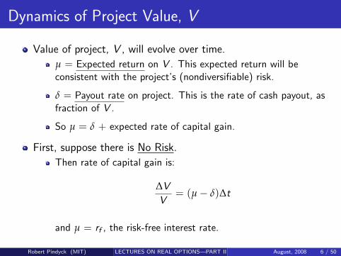
Dynamics of Project Value, V
Value of project, V , will evolve over time.
µ = Expected return on V . This expected return will beconsistent with the project’s (nondiversifiable) risk.
δ = Payout rate on project. This is the rate of cash payout, asfraction of V .
So µ = δ + expected rate of capital gain.
First, suppose there is No Risk.
Then rate of capital gain is:
∆V
V= (µ− δ)∆t
and µ = rf , the risk-free interest rate.
Robert Pindyck (MIT) LECTURES ON REAL OPTIONS—PART II August, 2008 6 / 50

Dynamics of Project Value, V (Continued)
Now, suppose V is risky. Then:
∆V
V= (µ− δ)∆t + σet
where et is random, zero-mean. So V follows a random walk, like theprice of a stock.
If all risk is diversifiable, µ = rf .
If there is nondiversifiable risk, µ > rf .
Formally, write process for V as:
dV
V= (µ− δ)dt + σdz
where dz = et
√dt is the increment of a Wiener process, and et
normally distributed, with (dz)2 = dt.
So V follows a geometric Brownian motion (GBM).
Note (dV )2 = σ2V 2dt.
Robert Pindyck (MIT) LECTURES ON REAL OPTIONS—PART II August, 2008 7 / 50

Mathematical Background
Wiener Process: If z(t) is a Wiener process, any change in z ,∆z , over time interval ∆t, satisfies
1. The relationship between ∆z and ∆t is given by:
∆z = εt
√∆t,
where εt is a normally distributed random variable with zeromean and a standard deviation of 1.
2. The random variable εt is serially uncorrelated, i.e., E [εtεs ] = 0for t 6= s. Thus values of ∆z for any two different time intervalsare independent.
Robert Pindyck (MIT) LECTURES ON REAL OPTIONS—PART II August, 2008 8 / 50

Mathematical Background (continued)
What do these conditions imply for change in z over an intervalof time T?
Break interval up into n units of length ∆t each, withn = T /∆t. Then the change in z over this interval is
z(s + T )− z(s) =n
∑i=1
εi
√∆t (1)
The εi ’s are independent of each other. By the Central LimitTheorem, the change z(s + T )− z(s) is normally distributedwith mean 0 and variance n ∆t = T .
This result, which follows from the fact that ∆z depends on√∆t and not on ∆t, is particularly important; the variance of
the change in a Wiener process grows linearly with the timehorizon.
Robert Pindyck (MIT) LECTURES ON REAL OPTIONS—PART II August, 2008 9 / 50

Mathematical Background (continued)
By letting ∆t become infinitesimally small, we can represent theincrement of a Wiener process, dz , as:
dz = εt
√dt (2)
Since εt has zero mean and unit standard deviation, E(dz) = 0,and V [dz ] = E [(dz)2] = dt.Note that a Wiener process has no time derivative in aconventional sense; ∆z/∆t = εt (∆t)−1/2, which becomesinfinite as ∆t approaches zero.
Generalization: Brownian Motion with Drift.
dx = α dt + σ dz , (3)
where dz is the increment of a Wiener process, α is the driftparameter, and σ the variance parameter.
Robert Pindyck (MIT) LECTURES ON REAL OPTIONS—PART II August, 2008 10 / 50

Mathematical Background (continued)
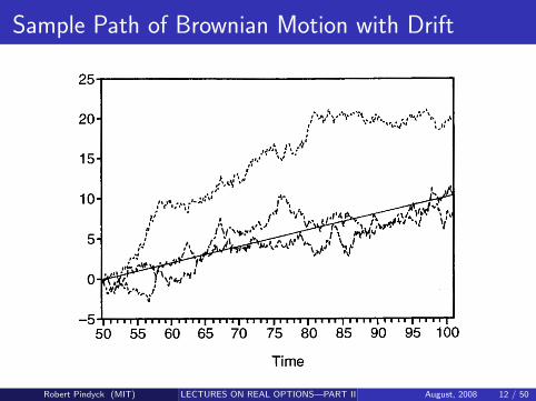
Over any time interval ∆t, ∆x is normally distributed, and hasexpected value E(∆x) = α ∆t and variance V(∆x) = σ2∆t.
Figure 1 shows three sample paths of eq. (3), with α = 0.2 peryear, and σ = 1.0 per year. Each sample path was generated bytaking a ∆t of one month, and then calculating a trajectory forx(t) using
xt = xt−1 + .01667 + .2887 εt , (4)
with x1950 = 0. In eq. (4), at each time t, εt is drawn from anormal distribution with zero mean and unit standard deviation.(Note: α and σ are in monthly terms. Trend of .2 per yearimplies 0.0167 per month; S.D. of 1.0 per year implies varianceof 1.0 per year, hence variance of 1
12 = .0833 per month, so
monthly S.D. is√
0.0833 = 0.2887.) Also shown is a trend line,i.e., eq. (4) with εt = 0.
Robert Pindyck (MIT) LECTURES ON REAL OPTIONS—PART II August, 2008 11 / 50
Sample Path of Brownian Motion with Drift
Robert Pindyck (MIT) LECTURES ON REAL OPTIONS—PART II August, 2008 12 / 50

Mathematical Background (continued)
Fig. 2 shows a forecast of this process. A sample path wasgenerated from 1950 to the end of 1974, again using eq. (4),and then forecasts of x(t) were constructed for 1975 to 2000.The forecast of x for T months beyond Dec. 1974 is
x̂1974+T = x1974 + .01667 T .
The graph also shows a 66 percent forecast confidence interval,i.e., the forecasted x(t) plus or minus one standard deviation.Recall that variance grows linearly with the time horizon, so thestandard deviation grows as the square root of the time horizon.Hence the 66 percent confidence interval is
x1974 + .01667T ± .2887√
T .
One can similarly construct 90 or 95 percent confidence intervals.
Robert Pindyck (MIT) LECTURES ON REAL OPTIONS—PART II August, 2008 13 / 50

Forecast of Brownian Motion with Drift
Robert Pindyck (MIT) LECTURES ON REAL OPTIONS—PART II August, 2008 14 / 50

Mathematical Background (continued)
Generalized Brownian Motion: Ito Process.
dx = a(x , t)dt + b(x , t)dz
Mean of dx : E(dz) = 0 so E(dx) = α(x , t)dt.
Variance of dx : V(dx) = E [dx2]− (E [dx ]2), which hass termsin dt, (dt)2, and (dt)(dz), which is of order (dt)3/2. For dtinfinitesimally small, terms in (dt)2 and (dt)3/2 can be ignored,so
V [dx ] = b2(x , t) dt.
Geometric Brownian Motion (GBM).
a(x , t) = αx , and b(x , t) = σx , so
dx = α x dt + σ x dz . (5)
Percentage changes in x , ∆x/x , are normally distributed, soabsolute changes in x , ∆x , are lognormally distributed.
Robert Pindyck (MIT) LECTURES ON REAL OPTIONS—PART II August, 2008 15 / 50

Mathematical Background (continued)
If x(0) = x0, the expected value of x(t) is
E [x(t)] = x0 eαt ,
and the variance of x(t) is
V [x(t)] = x20 e2αt (eσ2 t − 1).
We can calculate the expected present discounted value of x(t)over some period of time. For example,
E[ ∫ ∞
0x(t) e−rt dt
]=
∫ ∞
0x0 e−(r−α)t dt = x0/(r − α) .
(6)
Robert Pindyck (MIT) LECTURES ON REAL OPTIONS—PART II August, 2008 16 / 50

Mathematical Background (continued)
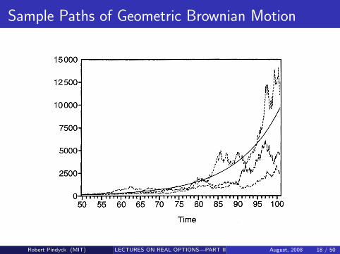
Fig. 3 shows three sample paths of eq. (5), with α = .09 andσ = .2. (These numbers approximately equal annual expectedgrowth rate and S.D. of the NYSE Index in real terms.) Samplepaths were generated by taking a ∆t of one month, and using
xt = 1.0075 xt−1 + .0577 xt−1 εt , (7)
with x1950 = 100. Also shown is the trend line.
Note that in one of these sample paths the “stock market”outperformed its expected rate of growth, but in the other two itunderperformed.
Robert Pindyck (MIT) LECTURES ON REAL OPTIONS—PART II August, 2008 17 / 50
Sample Paths of Geometric Brownian Motion
Robert Pindyck (MIT) LECTURES ON REAL OPTIONS—PART II August, 2008 18 / 50

Mathematical Background (continued)
Figure 4 shows a forecast of this process. The forecasted valueof x is given by
x̂1974+T = (1.0075)T x1974 ,
where T is in months. Also shown is a 66-percent confidenceinterval. Since the S.D. of percentage changes in x grows withthe square root of the time horizon, bounds of this confidenceinterval are
(1.0075)T (1.0577)√
T x1974 and (1.0075)T (1.0577)−√
T x1974 .
Robert Pindyck (MIT) LECTURES ON REAL OPTIONS—PART II August, 2008 19 / 50

Forecast of Geometric Brownian Motion
Robert Pindyck (MIT) LECTURES ON REAL OPTIONS—PART II August, 2008 20 / 50

Mathematical Background (continued)
Mean-Reverting Processes: Simplest is
dx = η (x̄ − x) dt + σ dz . (8)
Here, η is speed of reversion, and x̄ is “normal” level of x .
If x = x0, its expected value at future time t is
E [xt ] = x̄ + (x0 − x̄) e−ηt . (9)
Also, the variance of (xt − x̄) is
V [xt − x̄ ] =σ2
2η(1− e−2ηt). (10)
Note that E [xt ] → x̄ as t becomes large, and variance→ σ2/2η. Also, as η → ∞, V [xt ] → 0, so x can never deviatefrom x̄ . As η → 0, x becomes a simple Brownian motion, andV [xt ] → σ2 t.
Robert Pindyck (MIT) LECTURES ON REAL OPTIONS—PART II August, 2008 21 / 50

Mathematical Background (continued)
Fig. 5 shows four sample paths of equation (8) for differentvalues of η. In each case, σ = .05 in monthly terms, x̄ = 1, andx(t) begins at x0 = 1.
Fig. 6 shows an optimal forecast for η = .02, along with a66-percent confidence interval. Note that after four or five years,the variance of the forecast converges toσ2/2η = .0025/.04 = .065, so the 66 percent confidenceinterval (± 1 S.D.) converges to the forecast ±.25.
Robert Pindyck (MIT) LECTURES ON REAL OPTIONS—PART II August, 2008 22 / 50

Sample Paths of Mean-Reverting Process
dx = η (x̄ − x) dt + σ dz
Robert Pindyck (MIT) LECTURES ON REAL OPTIONS—PART II August, 2008 23 / 50
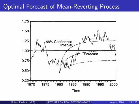
Optimal Forecast of Mean-Reverting Process
Robert Pindyck (MIT) LECTURES ON REAL OPTIONS—PART II August, 2008 24 / 50

Mathematical Background (continued)
Can generalize eq. (8). For example, one might expect x(t) torevert to x̄ but the variance rate to grow with x . Then one coulduse
dx = η (x̄ − x) dt + σ x dz . (11)
Or, proportional changes in a variable might be modelled asmean- reverting:
dx = η x (x̄ − x) dt + σ x dz . (12)
Robert Pindyck (MIT) LECTURES ON REAL OPTIONS—PART II August, 2008 25 / 50

Mathematical Background (continued)
Ito’s Lemma: Suppose x(t) is an Ito process, i.e.,
dx = a(x , t)dt + b(x , t)dz , (13)
How do we take derivatives of F (x , t)?Usual rule of calculus:
dF =∂F
∂xdx +
∂F
∂tdt.
But suppose we include higher order terms:
dF =∂F
∂xdx +
∂F
∂tdt + 1
2
∂2F
∂x2(dx)2 + 1
6
∂3F
∂x3(dx)3 + ... (14)
Robert Pindyck (MIT) LECTURES ON REAL OPTIONS—PART II August, 2008 26 / 50
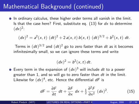
Mathematical Background (continued)
In ordinary calculus, these higher order terms all vanish in the limit.Is that the case here? First, substitute eq. (13) for dx to determine(dx)2:
(dx)2 = a2(x , t) (dt)2 + 2 a(x , t) b(x , t) (dt)3/2 + b2(x , t) dt.
Terms in (dt)3/2 and (dt)2 go to zero faster than dt as it becomesinfinitesimally small, so we can ignore these terms and write
(dx)2 = b2(x , t) dt.
Every term in the expansion of (dx)3 will include dt to a powergreater than 1, and so will go to zero faster than dt in the limit.Likewise for (dx)4, etc. Hence the differential dF is
dF =∂F
∂tdt +
∂F
∂xdx + 1
2
∂2F
∂x2(dx)2. (15)
Robert Pindyck (MIT) LECTURES ON REAL OPTIONS—PART II August, 2008 27 / 50
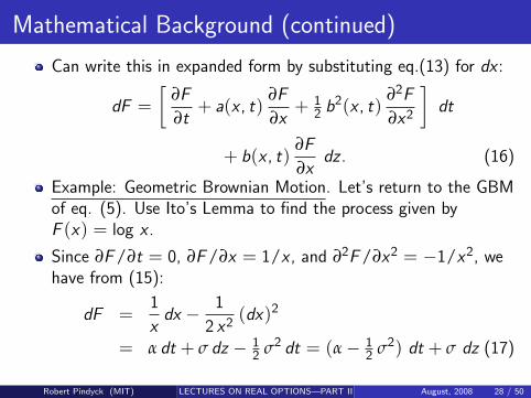
Mathematical Background (continued)
Can write this in expanded form by substituting eq.(13) for dx :
dF =[
∂F
∂t+ a(x , t)
∂F
∂x+ 1
2 b2(x , t)∂2F
∂x2
]dt
+ b(x , t)∂F
∂xdz . (16)
Example: Geometric Brownian Motion. Let’s return to the GBMof eq. (5). Use Ito’s Lemma to find the process given byF (x) = log x .
Since ∂F /∂t = 0, ∂F /∂x = 1/x , and ∂2F /∂x2 = −1/x2, wehave from (15):
dF =1
xdx − 1
2 x2(dx)2
= α dt + σ dz − 12 σ2 dt = (α− 1
2 σ2) dt + σ dz (17)
Robert Pindyck (MIT) LECTURES ON REAL OPTIONS—PART II August, 2008 28 / 50

Mathematical Background (continued)
Hence over any interval T , the change in log x is normallydistributed with mean (α− 1
2 σ2) T and variance σ2 T .
Why is the drift rate of F (x) = log x less than α? Becauselog x is a concave function of x , so with x uncertain, expectedvalue of log x changes by less than the log of the expected valueof x . Uncertainty over x is greater the longer the time horizon,so the expected value of log x is reduced by an amount thatincreases with time; hence drift rate is reduced.
Robert Pindyck (MIT) LECTURES ON REAL OPTIONS—PART II August, 2008 29 / 50

Investment Problem
Invest I , get V , with V a GBM, i.e.,
dV = αVdt + σVdz (18)
Payout rate is δ and expected rate of return is µ, so α = µ− δ.
Want value of the investment opportunity (i.e., the option toinvest), F (V ), and decision rule V ∗.Solution by Dynamic Programming: F (V ) must satisfy Bellmanequation:
ρ F dt = E(dF ) . (19)
This just says that over interval dt, total expected return on theinvestment opportunity, ρ F dt, is equal to expected rate ofcapital appreciation.Expand dF using Ito’s Lemma:
dF = F ′(V ) dV + 12 F ′′(V ) (dV )2 .
Robert Pindyck (MIT) LECTURES ON REAL OPTIONS—PART II August, 2008 30 / 50

Investment Problem (continued)
Substituting eq. (18) for dV and noting that E(dz) = 0 gives
E [dF ] = α V F ′(V ) dt + 12 σ2 V 2 F ′′(V ) dt .
Hence the Bellman equation becomes (after dividing through by dt):
12 σ2 V 2 F ′′(V ) + α V F ′(V )− ρ F = 0 . (20)
Also, F (V ) must satisfy boundary conditions:
F (0) = 0 (21)
F (V ∗) = V ∗ − I (22)
F ′(V ∗) = 1 (23)
This is easy to solve, but first, let’s do this again using option pricingapproach. Then we avoid problem of choosing ρ and α.
Robert Pindyck (MIT) LECTURES ON REAL OPTIONS—PART II August, 2008 31 / 50

Investment Problem (continued)
Solution by Contingent Claims Analysis.Create a risk-free portfolio: Hold option to invest, worth F (V ).Short n = dF /dV units of project.
Value of portfolio = Φ = F − F ′(V )V
Short position requires payment of δVF ′(V ) dollars per period.So total return on portfolio is:
dF − F ′(V )dV − δVF ′(V )dt
Since dF = F ′(V )dV + 12F ′′(V )(dV )2, total return is:
12F ′′(V )(dV )2 − δVF ′(V )dt
(dV )2 = σ2V 2dt, so total return becomes:
12σ2V 2F ′′(V )dt − δVF ′(V )dt
Robert Pindyck (MIT) LECTURES ON REAL OPTIONS—PART II August, 2008 32 / 50
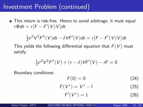
Investment Problem (continued)
This return is risk-free. Hence to avoid arbitrage, it must equalrΦdt = r [F − F ′(V )V ]dt:
12σ2V 2F ′′(V )dt − δVF ′(V )dt = r [F − F ′(V )V ]dt
This yields the following differential equation that F (V ) mustsatisfy:
12σ2V 2F ′′(V ) + (r − δ)VF ′(V )− rF = 0
Boundary conditions:F (0) = 0 (24)
F (V ∗) = V ∗ − I (25)
F ′(V ∗) = 1 (26)
Robert Pindyck (MIT) LECTURES ON REAL OPTIONS—PART II August, 2008 33 / 50

Investment Problem (continued)
Solution. You can check (by substitution) that
F (V ) = AV β, for V ≤ V ∗
= V − I , for V > V ∗
where β = 12 −
r − δ
σ2+
√(r − δ
σ2− 1
2
)2
+2r
σ2,
V ∗ =βI
β− 1, A =
V ∗ − I
(V ∗)β
Solution is shown in figure.
Robert Pindyck (MIT) LECTURES ON REAL OPTIONS—PART II August, 2008 34 / 50

Graph of F (V )
Robert Pindyck (MIT) LECTURES ON REAL OPTIONS—PART II August, 2008 35 / 50

Characteristics of Solution
Higher σ: Makes F larger, and also makes V ∗ larger. Now thefirm’s options to invest (patents, land, etc.) are worth more, butthe firm should do less investing. Opportunity cost of investingis higher.
Higher δ: Higher cash payout rate increases opportunity cost ofkeeping the option alive. Makes F smaller, V ∗ smaller. Now thefirm’s options to invest are worth less, but the firm should domore investing.
Higher r : Makes F larger and V ∗ larger. Option value increasesbecause present value of exercise price I decreases (in event ofexercise). This increases opportunity cost of “killing” the option,so V ∗ rises.
Robert Pindyck (MIT) LECTURES ON REAL OPTIONS—PART II August, 2008 36 / 50

Characteristics of Solution (continued)
Higher I : Makes F smaller and V ∗ larger. Note that as I → 0,F → V , and V ∗ → 0.
Question: Suppose σ increases. We know this makes V ∗ larger.What happens to E(T ∗), the expected time until V reaches V ∗
and investment occurs?
The following two figures illustrate how F (V ) and V ∗ vary withσ and δ.
Robert Pindyck (MIT) LECTURES ON REAL OPTIONS—PART II August, 2008 37 / 50

Value of Investment Opportunity
Robert Pindyck (MIT) LECTURES ON REAL OPTIONS—PART II August, 2008 38 / 50

Critical Value V ∗ as a Function of σ
Robert Pindyck (MIT) LECTURES ON REAL OPTIONS—PART II August, 2008 39 / 50

How Important is Option Value?
Take a factory which costs $1 million (= I ) to build. Supposeriskless rate is 7% (nominal). Critical value V ∗ is shown belowfor different values of σ and δ.
Payout Rate δ2% 5% 10% 15%
Annual 10% 3.84 1.65 1.13 1.06Standard Deviation 20% 4.77 2.15 1.40 1.22
of Project Value (σ) 40% 8.06 3.61 2.18 1.73
For average firm on NYSE, σ = 20%.
Observe that for σ = 20% or 40%, V ∗ is much larger than I . Sohow important is option value? Very.
Robert Pindyck (MIT) LECTURES ON REAL OPTIONS—PART II August, 2008 40 / 50
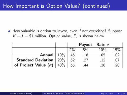
How Important is Option Value? (continued)
How valuable is option to invest, even if not exercised? SupposeV = I = $1 million. Option value, F , is shown below.
Payout Rate δ2% 5% 10% 15%
Annual 10% .46 .18 .05 .02Standard Deviation 20% .52 .27 .12 .07
of Project Value (σ) 40% .65 .44 .28 .20
Robert Pindyck (MIT) LECTURES ON REAL OPTIONS—PART II August, 2008 41 / 50

Mean-Reverting Process
Suppose V follows the mean-reverting process:
dV = η (V̄ − V ) V dt + σ V dz , (27)
To find the optimal investment rule, we will use contingentclaims analysis.
Let µ = risk-adjusted discount rate for project.
Expected rate of growth of V is not constant, but a function ofV . Hence the “shortfall,” δ = µ− (1/dt)E(dV )/V , is afunction of V :
δ(V ) = µ− η (V̄ − V ) . (28)
The differential equation for F (V ) is now
12 σ2 V 2 F ′′(V ) + [r − µ + η (V̄ − V )] V F ′(V )− r F = 0 .
(29)Also, F (V ) must satisfy the same boundary conditions (21) –(23) as before, and for the same reasons.
Robert Pindyck (MIT) LECTURES ON REAL OPTIONS—PART II August, 2008 42 / 50

Mean-Reverting Process (continued)
Solution is a little more complicated. Define a new functionh(V ) by
F (V ) = A V θ h(V ) , (30)
Substituting this into eq. (29) and rearranging gives thefollowing equation:
V θ h(V )[
12 σ2 θ(θ − 1) + (r − µ + η V̄ ) θ − r
]+ V θ+1
[12 σ2 V h′′(V ) + (σ2θ + r − µ + η V̄ − η V ) h′(V )
− η θ h(V )] = 0 . (31)
Robert Pindyck (MIT) LECTURES ON REAL OPTIONS—PART II August, 2008 43 / 50

Mean-Reverting Process (continued)
Eq. (31) must hold for any value of V , so the bracketed termsin both the first and second lines must equal zero. First chooseθ to set the bracketed terms in the first line equal to zero:
12 σ2 θ(θ − 1) + (r − µ + η V̄ ) θ − r = 0 .
To satisfy the boundary condition that F (0) = 0, we use thepositive solution:
θ = 12 +(µ− r − ηV̄ )/σ2 +
√[(r − µ + ηV̄ )/σ2 − 1
2
]2 + 2r/σ2 .(32)
From the second line of eq. (31),
12 σ2 V h′′(V )+ (σ2 θ + r −µ + η V̄ − η V ) h′(V )− η θ h(V ) = 0 .
(33)
Robert Pindyck (MIT) LECTURES ON REAL OPTIONS—PART II August, 2008 44 / 50

Mean-Reverting Process (continued)
Make the substitution x = 2ηV /σ2, to transform eq.(33) into astandard form. Let h(V ) = g(x), so that h′(V ) = (2η/σ2) g ′(x)and h′′(V ) = (2η/σ2)2 g ′′(x). Then (33) becomes
x g ′′(x) + (b− x) g ′(x)− θ g(x) = 0 , (34)
whereb = 2θ + 2 (r − µ + ηV̄ )/σ2 .
Eq. (34) is Kummer’s Equation. Its solution is the confluenthypergeometric function H(x ; θ, b(θ)), which has the followingseries representation:
H(x ; θ, b) = 1+θ
bx +
θ(θ + 1)b(b + 1)
x2
2!+
θ(θ + 1)(θ + 2)b(b + 1)(b + 2)
x3
3!+ . . . .
(35)
Robert Pindyck (MIT) LECTURES ON REAL OPTIONS—PART II August, 2008 45 / 50

Mean-Reverting Process (continued)
We have verified that the solution to equation (29) is indeed ofthe form of equation (30). Solution is
F (V ) = A V θ H(2η
σ2V ; θ, b) , (36)
where A is a constant yet to be determined.
We can find A, as well as the critical value V ∗, from theremaining two boundary conditions, that is, F (V ∗) = V ∗ − Iand FV (V ∗) = 1. Because the confluent hypergeometricfunction is an infinite series, A and V ∗ must be foundnumerically.
Look at several numerical solutions. Set I = 1, r = .04,µ = .08, and σ = .2. We will vary η and V̄ .
Robert Pindyck (MIT) LECTURES ON REAL OPTIONS—PART II August, 2008 46 / 50
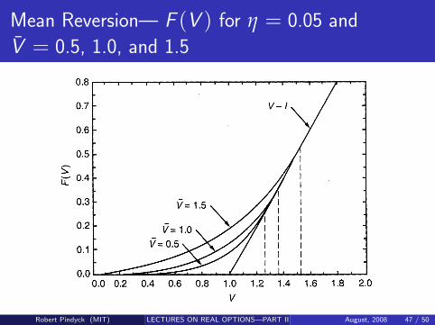
Mean Reversion— F (V ) for η = 0.05 and
V̄ = 0.5, 1.0, and 1.5
Robert Pindyck (MIT) LECTURES ON REAL OPTIONS—PART II August, 2008 47 / 50

Mean Reversion— F (V ) for η = 0.1 and
V̄ = 0.5, 1.0, and 1.5
Robert Pindyck (MIT) LECTURES ON REAL OPTIONS—PART II August, 2008 48 / 50

Mean Reversion— F (V ) for η = 0.5 and
V̄ = 0.5, 1.0, and 1.5
Robert Pindyck (MIT) LECTURES ON REAL OPTIONS—PART II August, 2008 49 / 50

Crtical Value V ∗ as a Function of η for µ = 0.08
and V̄ = 0.1, 1.0, and 1.5
Robert Pindyck (MIT) LECTURES ON REAL OPTIONS—PART II August, 2008 50 / 50