From Robotic Routing and Balancingto Stochastic Surveillance

Francesco Bullo

Center for Control,Dynamical Systems & Computation

University of California at Santa Barbara

http://motion.me.ucsb.edu

System and Control DepartmentIndian Institute of Technology Bombay, Jan 4, 2017

Acknowledgments

Jorge Cortes∗

Sonia Martınez∗

Emilio Frazzoli∗

Marco Pavone∗

Paolo Frasca∗

G. NotarstefanoAnurag GanguliKetan SavlaRuggero Carli∗

Sara Susca

Stephen SmithShaunak BopardikarKarl ObermeyerJoey DurhamVaibhav Srivastava

Fabio PasqualettiRush PatelPushkarini AgharkarJeff PetersMishel George

Rush Patel,NorthropGrumman

PushkariniAgharkar,

SecreteCorporation

Mishel George,UCSB

VaibhavSrivastava,

Michigan State

Andrea Carron,ETH Zurich

NSF AFOSR ARO ONR DOE

New text “Lectures on Robotic Planning and Kinematics”

Lectures on Robotic Planning and Kinematics, ver .91For students: free PDF for downloadFor instructors: slides and answer keyshttp://motion.me.ucsb.edu/book-lrpk/

Robotic Planning:

1 Sensor-based planning

2 Motion planning via decomposition and search

3 Configuration spaces

4 Sampling and collision detetion

5 Motion planning via sampling

Robotic Kinematics:

6 Intro to kinematics

7 Rotation matrices

8 Displacement matrices and inverse kinematics

9 Linear and angular velocities

New text “Lectures on Network Systems”

Lectures onNetwork Systems

Francesco Bullo

With contributions byJorge Cortés

Florian DörflerSonia Martínez

Lectures on Network Systems, ver .85For students: free PDF for downloadFor instructors: slides and answer keyshttp://motion.me.ucsb.edu/book-lns/

Linear Systems:

1 motivating examples from social, sensor andcompartmental networks,

2 matrix and graph theory, with an emphasis onPerron–Frobenius theory and algebraic graph theory,

3 averaging algorithms in discrete and continuous time,described by static and time-varying matrices, and

4 positive and compartmental systems, described byMetzler matrices.

Nonlinear Systems:

5 formation control problems for robotic networks,

6 coupled oscillators, with an emphasis on theKuramoto model and models of power networks, and

7 virus propagation models, including lumped andnetwork models as well as stochastic anddeterministic models, and

8 population dynamic models in multi-species systems.

Stochastic surveillance and dynamic routing

Design efficient vehicle control strategies to

1 search unpredictably

2 detect anomalies quickly

3 provide service to customers at known locations

4 perform load balancing among vehicles

VehicleRouting

StochasticSurveillance

DataAggregation

Outline

1 vehicle routing2 load balancing and partitioning

3 stochastic surveillance

AeroVironment Inc, “Raven”unmanned aerial vehicle

iRobot Inc, “PackBot”unmanned ground vehicle

Vehicle routing in dynamic stochastic environments

customers appear sequentially randomly space/time

robotic network knows locations and provides service

Goal: distributed adaptive algos, delay vs throughput

F. Bullo, E. Frazzoli, M. Pavone, K. Savla, and S. L. Smith. Dynamic vehicle routingfor robotic systems. Proceedings of the IEEE, 99(9):1482–1504, 2011.

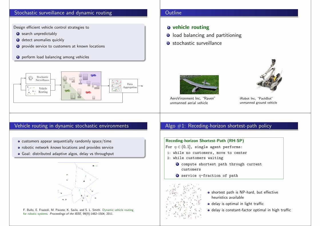
Algo #1: Receding-horizon shortest-path policy

Receding-horizon Shortest-Path (RH-SP)

For η ∈ (0, 1], single agent performs:

1: while no customers, move to center

2: while customers waiting

1 compute shortest path through current

customers

2 service η-fraction of path

shortest path is NP-hard, but effectiveheuristics available

delay is optimal in light traffic

delay is constant-factor optimal in high traffic

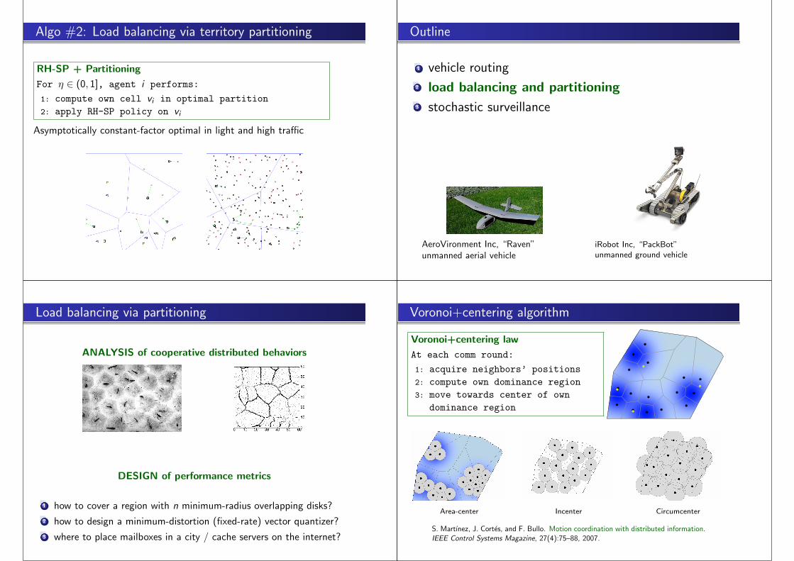
Algo #2: Load balancing via territory partitioning

RH-SP + Partitioning

For η ∈ (0, 1], agent i performs:

1: compute own cell vi in optimal partition

2: apply RH-SP policy on vi

Asymptotically constant-factor optimal in light and high traffic

Outline

1 vehicle routing

2 load balancing and partitioning3 stochastic surveillance

AeroVironment Inc, “Raven”unmanned aerial vehicle

iRobot Inc, “PackBot”unmanned ground vehicle

Load balancing via partitioning

ANALYSIS of cooperative distributed behaviors

DESIGN of performance metrics

1 how to cover a region with n minimum-radius overlapping disks?

2 how to design a minimum-distortion (fixed-rate) vector quantizer?

3 where to place mailboxes in a city / cache servers on the internet?

Voronoi+centering algorithm

Voronoi+centering law

At each comm round:

1: acquire neighbors’ positions

2: compute own dominance region

3: move towards center of own

dominance region

Area-center Incenter Circumcenter

S. Martınez, J. Cortes, and F. Bullo. Motion coordination with distributed information.IEEE Control Systems Magazine, 27(4):75–88, 2007.

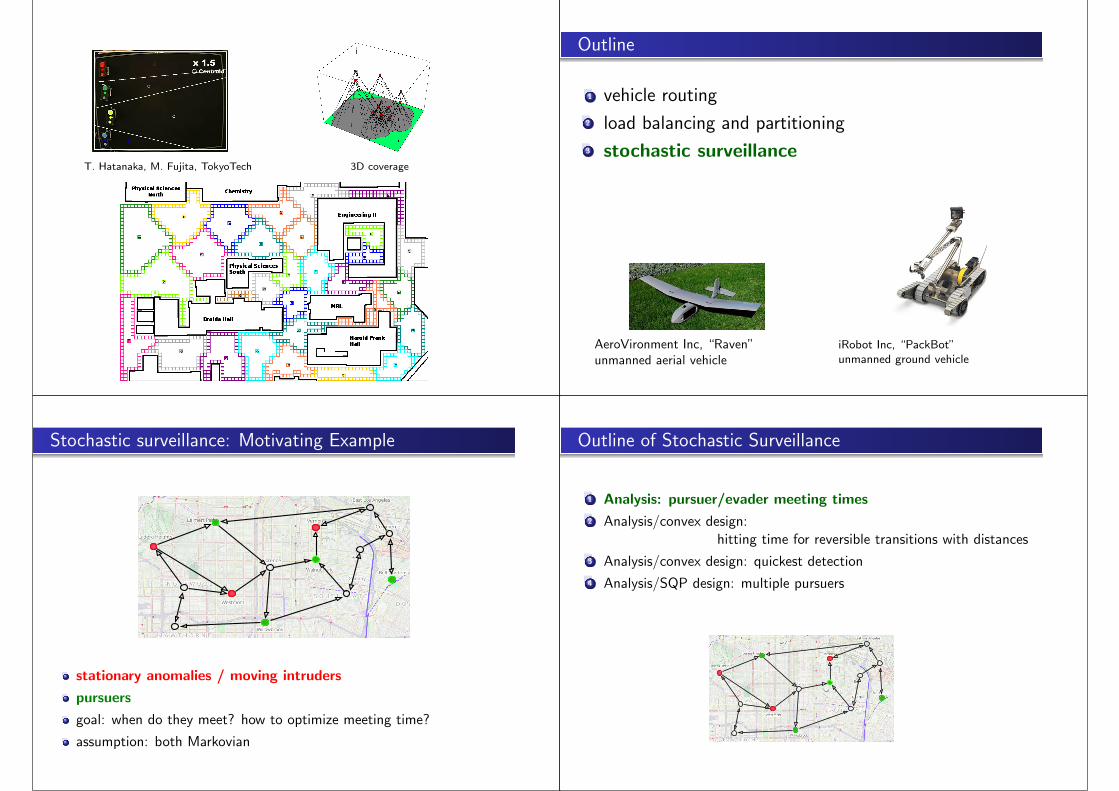
T. Hatanaka, M. Fujita, TokyoTech 3D coverage

Outline

1 vehicle routing

2 load balancing and partitioning

3 stochastic surveillance

AeroVironment Inc, “Raven”unmanned aerial vehicle

iRobot Inc, “PackBot”unmanned ground vehicle

Stochastic surveillance: Motivating Example

stationary anomalies / moving intruders

pursuers

goal: when do they meet? how to optimize meeting time?

assumption: both Markovian

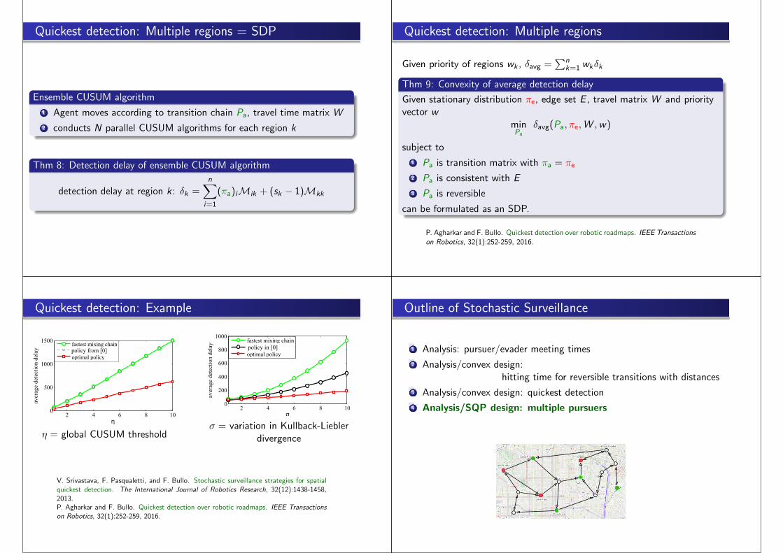
Outline of Stochastic Surveillance

1 Analysis: pursuer/evader meeting times

2 Analysis/convex design:hitting time for reversible transitions with distances

3 Analysis/convex design: quickest detection

4 Analysis/SQP design: multiple pursuers

Single pursuer/evader expected first meeting time

Mij(Pp,Pe) = E[first time pursuer starting @i meets evader starting @j]

?optimal

pursuer chain Pp?evader chain Pe

Objective

Given evader chain Pe

minpursuer chain Pp

E[Mij(Pp,Pe)]

Walks in the Kronecker graph

1

3 2

1

3 2

1,1

3,3 2,2

1,3

3,2 2,1

1,2

3,1 2,3

Pe

Pp

Pp ⌦ Pe

Thm 1: equivalent statements

(i) all Mij are finite(ii) from every (pursuer node, evader node) in Kronecker

graph there is a walk to a common node

The Kronecker product of matrices A ∈ Rn×m and B ∈ Rq×r is annq ×mr matrix given by

A⊗B =

a1,1B . . . a1,mB...

. . ....

an,1B. . . an,mB

Properties of the Kronecker product

Given the matrices A,B,C and D of appropriate dimensions,

(i) (A⊗B) is bilinear in A and B,

(ii) (A⊗B)(C ⊗D) = (AC )⊗(BD),

(iii) (B>⊗A) vec(C ) = vec(ACB),

where vec(C ) is the vectorization of C by stacking of the columns

Walks in the Kronecker graph — or lack thereof

1

3 2

1

3 2

1,1

3,3 2,2

1,3

3,2 2,1

1,2

3,1 2,3

Pe

Pp

Pp ⌦ Pe

1

3 2

1

3 2

1,1

3,3 2,2

1,3

3,2 2,1

1,2

3,1 2,3

Pe

Pp

Pp ⌦ Pe

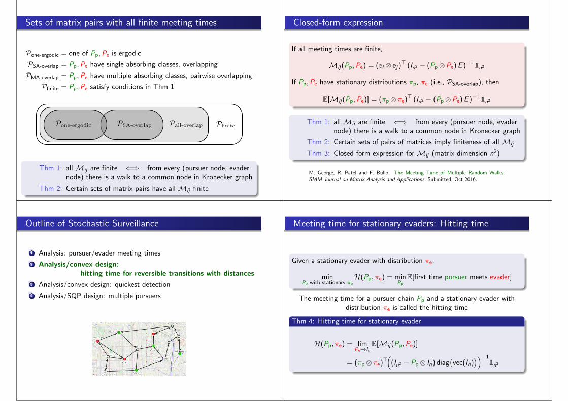
Sets of matrix pairs with all finite meeting times

Pone-ergodic = one of Pp,Pe is ergodic

PSA-overlap = Pp,Pe have single absorbing classes, overlapping

PMA-overlap = Pp,Pe have multiple absorbing classes, pairwise overlapping

Pfinite = Pp,Pe satisfy conditions in Thm 1

PfinitePSA-overlap Pall-overlapPone-ergodic

Thm 1: all Mij are finite ⇐⇒ from every (pursuer node, evadernode) there is a walk to a common node in Kronecker graph

Thm 2: Certain sets of matrix pairs have all Mij finite

Closed-form expression

If all meeting times are finite,

Mij(Pp,Pe) = (ei ⊗ ej)> (In2 − (Pp⊗Pe)E )−1 1n2

If Pp,Pe have stationary distributions πp, πe (i.e., PSA-overlap), then

E[Mij(Pp,Pe)] = (πp⊗πe)> (In2 − (Pp⊗Pe)E )−1 1n2

Thm 1: all Mij are finite ⇐⇒ from every (pursuer node, evadernode) there is a walk to a common node in Kronecker graph

Thm 2: Certain sets of pairs of matrices imply finiteness of all Mij

Thm 3: Closed-form expression for Mij (matrix dimension n2)

M. George, R. Patel and F. Bullo. The Meeting Time of Multiple Random Walks.SIAM Journal on Matrix Analysis and Applications, Submitted, Oct 2016.

Outline of Stochastic Surveillance

1 Analysis: pursuer/evader meeting times

2 Analysis/convex design:hitting time for reversible transitions with distances

3 Analysis/convex design: quickest detection

4 Analysis/SQP design: multiple pursuers

Meeting time for stationary evaders: Hitting time

Given a stationary evader with distribution πe,

minPp with stationary πp

H(Pp, πe) = minPp

E[first time pursuer meets evader]

The meeting time for a pursuer chain Pp and a stationary evader withdistribution πe is called the hitting time

Thm 4: Hitting time for stationary evader

H(Pp, πe) = limPe→In

E[Mij(Pp,Pe)]

= (πp⊗πe)>(

(In2 − Pp⊗ In) diag(vec(In)

))−11n2

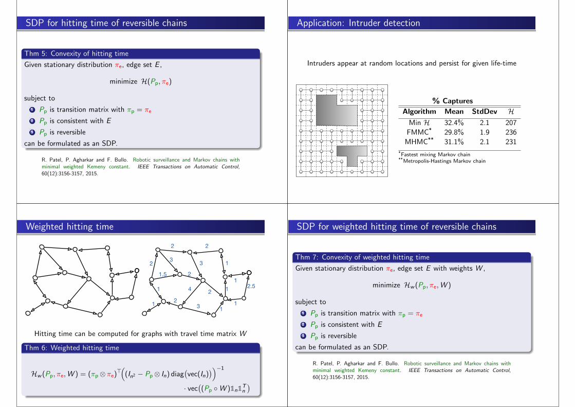
SDP for hitting time of reversible chains

Thm 5: Convexity of hitting time

Given stationary distribution πe, edge set E ,

minimize H(Pp, πe)

subject to

1 Pp is transition matrix with πp = πe

2 Pp is consistent with E

3 Pp is reversible

can be formulated as an SDP.

R. Patel, P. Agharkar and F. Bullo. Robotic surveillance and Markov chains withminimal weighted Kemeny constant. IEEE Transactions on Automatic Control,60(12):3156-3157, 2015.

Application: Intruder detection

Intruders appear at random locations and persist for given life-time

% Captures

Algorithm Mean StdDev HMin H 32.4% 2.1 207

FMMC* 29.8% 1.9 236

MHMC** 31.1% 2.1 231

*Fastest mixing Markov chain**Metropolis-Hastings Markov chain

Weighted hitting time

2 2

1

2.5

1

1

3

2

132

4

2

321.5

1

1

1

Hitting time can be computed for graphs with travel time matrix W

Thm 6: Weighted hitting time

Hw (Pp, πe,W ) = (πp⊗πe)>(

(In2 − Pp⊗ In) diag(vec(In)

))−1

· vec((Pp ◦W )1n1T

n

)

SDP for weighted hitting time of reversible chains

Thm 7: Convexity of weighted hitting time

Given stationary distribution πe, edge set E with weights W ,

minimize Hw (Pp, πe,W )

subject to

1 Pp is transition matrix with πp = πe

2 Pp is consistent with E

3 Pp is reversible

can be formulated as an SDP.

R. Patel, P. Agharkar and F. Bullo. Robotic surveillance and Markov chains withminimal weighted Kemeny constant. IEEE Transactions on Automatic Control,60(12):3156-3157, 2015.

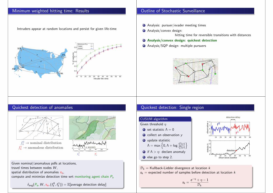
Minimum weighted hitting time: Results

Intruders appear at random locations and persist for given life-time

10 15 20 25 30 35 40 45 50 55 60

0.4

0.5

0.6

0.7

0.8

0.9

1

Intruder life−time

% o

f cap

ture

s

MinimumFMMCMHMC

Outline of Stochastic Surveillance

1 Analysis: pursuer/evader meeting times

2 Analysis/convex design:hitting time for reversible transitions with distances

3 Analysis/convex design: quickest detection

4 Analysis/SQP design: multiple pursuers

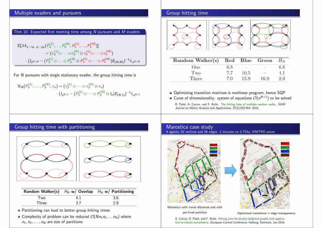
Quickest detection of anomalies

Given nominal/anomalous pdfs at locations,travel times between nodes W ,spatial distribution of anomalies πe,compute and minimize detection time wrt monitoring agent chain Pa

δavg(Pa,W , πe, (f0k , f

1k )) = E[average detection delay]

Quickest detection: Single region

CUSUM algorithm

Given threshold η

1 set statistic Λ = 0

2 collect an observation y

3 update statistic

Λ = max{

0,Λ + logf 1k (y)

f 0k (y)

}

4 if Λ > η: declare anomaly

5 else go to step 2.

10 20 30 40 50 60 70 80−4

−2

0

2

4

obse

rvat

ion

y

10 20 30 40 50 60 70 800

5

10

15

20

stat

isti

c Λ

detection

}detection delay

f0k

f1k

observation number

Dk = Kullback-Liebler divergence at location ksk = expected number of samples before detection at location k

sk =e−η + η − 1

Dk

Quickest detection: Multiple regions = SDP

Ensemble CUSUM algorithm

1 Agent moves according to transition chain Pa, travel time matrix W

2 conducts N parallel CUSUM algorithms for each region k

Thm 8: Detection delay of ensemble CUSUM algorithm

detection delay at region k: δk =n∑

i=1

(πa)iMik + (sk − 1)Mkk

Quickest detection: Multiple regions

Given priority of regions wk , δavg =∑n

k=1 wkδk

Thm 9: Convexity of average detection delay

Given stationary distribution πe, edge set E , travel matrix W and priorityvector w

minPa

δavg(Pa, πe,W ,w)

subject to

1 Pa is transition matrix with πa = πe

2 Pa is consistent with E

3 Pa is reversible

can be formulated as an SDP.

P. Agharkar and F. Bullo. Quickest detection over robotic roadmaps. IEEE Transactionson Robotics, 32(1):252-259, 2016.

Quickest detection: Example

2 4 6 8 100

500

1000

1500

η

aver

age

dete

ctio

n de

lay

fastest mixing chain

optimal policypolicy from [0]

η = global CUSUM threshold

2 4 6 8 100

200

400

600

800

1000

σ

aver

age

dete

ctio

n de

lay fastest mixing chain

policy in [0]optimal policy

σ = variation in Kullback-Lieblerdivergence

V. Srivastava, F. Pasqualetti, and F. Bullo. Stochastic surveillance strategies for spatialquickest detection. The International Journal of Robotics Research, 32(12):1438-1458,2013.P. Agharkar and F. Bullo. Quickest detection over robotic roadmaps. IEEE Transactionson Robotics, 32(1):252-259, 2016.

Outline of Stochastic Surveillance

1 Analysis: pursuer/evader meeting times

2 Analysis/convex design:hitting time for reversible transitions with distances

3 Analysis/convex design: quickest detection

4 Analysis/SQP design: multiple pursuers

Multiple evaders and pursuers

Thm 10: Expected first meeting time among N pursuers and M evaders

E[Mi1···iN , j1···jM (P(1)p ,. . .,P

(N)p ,P

(1)e ,. . .,P

(M)e )]

= (π(1)p ⊗ · · ·⊗π(N)

p ⊗π(1)e ⊗ · · ·⊗π(M)

e )

· (InN+M − (P(1)p ⊗ . . .⊗P

(N)P ⊗P

(1)e ⊗ · · ·⊗P

(M)e )E(N,M))−11nN+M

For N pursuers with single stationary evader, the group hitting time is

HN(P(1)p , . . . ,P

(N)p , πe) = (π

(1)p ⊗ · · ·⊗π(N)

p ⊗πe)

· (InN+1 − (P(1)p ⊗ · · ·⊗P

(N)p ⊗ In)E(N,1))−11nN+1

Group hitting time

Optimizing transition matrices is nonlinear program, hence SQP

Curse of dimensionality: system of equations O(nN+1) to be solved

R. Patel, A. Carron, and F. Bullo. The hitting time of multiple random walks. SIAMJournal on Matrix Analysis and Applications, 37(3):933-954, 2016.

Group hitting time with partitioning

Random Walker(s) HN w/ Overlap HN w/ Partitioning

Two 4.1 3.6Three 3.7 2.9

Partitioning can lead to better group hitting times

Complexity of problem can be reduced O(Nn1n2 . . . nN) wheren1, n2, . . . , nN are size of partitions

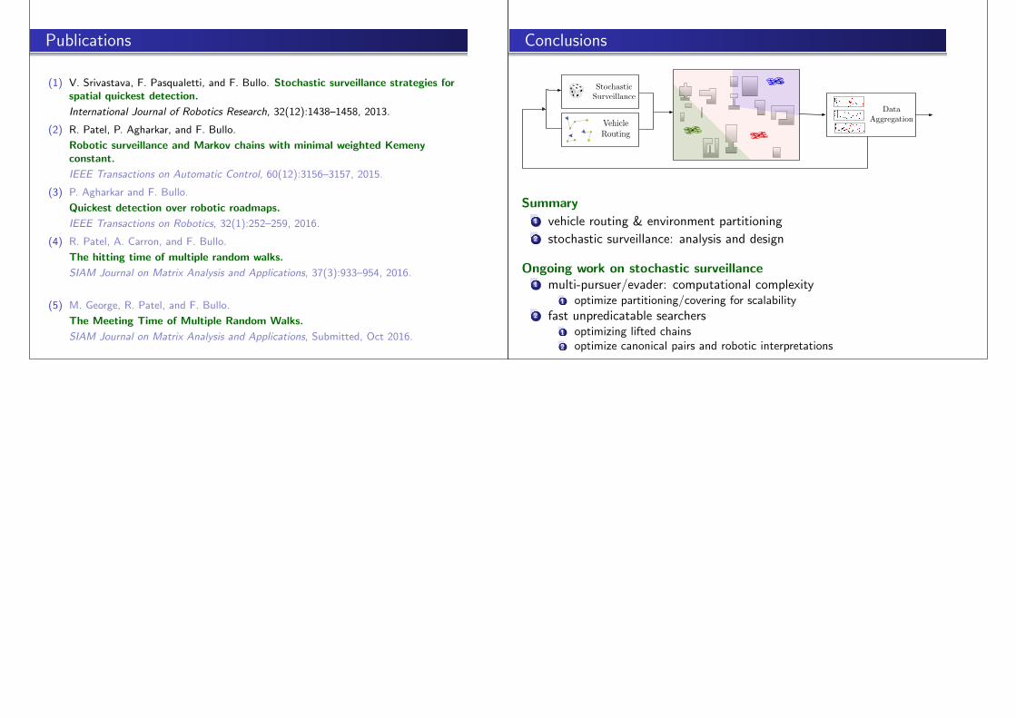
Marostica case study4 agents, 42 vertices and 56 edges: 2 minutes on 2.7Ghz, KNITRO solver

Marostica with travel distances and with

pre-fixed partition Optimized transitions ≈ edge transparency

A. Carron, R. Patel, and F. Bullo. Hitting time for doubly-weighted graphs with applica-tion to robotic surveillance. European Control Conference, Aalborg, Denmark, Jun 2016.

Publications

(1) V. Srivastava, F. Pasqualetti, and F. Bullo. Stochastic surveillance strategies forspatial quickest detection.

International Journal of Robotics Research, 32(12):1438–1458, 2013.

(2) R. Patel, P. Agharkar, and F. Bullo.

Robotic surveillance and Markov chains with minimal weighted Kemenyconstant.

IEEE Transactions on Automatic Control, 60(12):3156–3157, 2015.

(3) P. Agharkar and F. Bullo.

Quickest detection over robotic roadmaps.

IEEE Transactions on Robotics, 32(1):252–259, 2016.

(4) R. Patel, A. Carron, and F. Bullo.

The hitting time of multiple random walks.

SIAM Journal on Matrix Analysis and Applications, 37(3):933–954, 2016.

(5) M. George, R. Patel, and F. Bullo.

The Meeting Time of Multiple Random Walks.

SIAM Journal on Matrix Analysis and Applications, Submitted, Oct 2016.

Conclusions

VehicleRouting

StochasticSurveillance

DataAggregation

Summary1 vehicle routing & environment partitioning2 stochastic surveillance: analysis and design

Ongoing work on stochastic surveillance1 multi-pursuer/evader: computational complexity

1 optimize partitioning/covering for scalability2 fast unpredicatable searchers

1 optimizing lifted chains2 optimize canonical pairs and robotic interpretations