Lectures on L-functions, Converse Theorems, and Functoriality for GL

Lectures on L-functions, Converse Theorems, and

Functoriality for GLn

J.W. Cogdell

Department of Mathematics, Oklahoma State University, Stillwater OK 74078

Contents

Preface 1

Lecture 1. Modular Forms and Their L-functions 3

Lecture 2. Automorphic Forms 13

Lecture 3. Automorphic Representations 21

Lecture 4. Fourier Expansions and Multiplicity One Theorems 29

Lecture 5. Eulerian Integral Representations 37

Lecture 6. Local L-functions: the Non-Archimedean Case 45

Lecture 7. The Unramified Calculation 53

Lecture 8. Local L-functions: the Archimedean Case 61

Lecture 9. Global L-functions 69

Lecture 10. Converse Theorems 77

Lecture 11. Functoriality 87

Lecture 12. Functoriality for the Classical Groups 93

Lecture 13. Functoriality for the Classical Groups, II 99

iii

iv Contents

Preface

These are the lecture notes that accompanied my lecture series at the FieldsInstitute in the Spring of 2003 as part of the Thematic Program on AutomorphicForms. The posted description of the course was the following.

“The theory of L-functions of automorphic forms (or modular forms) via in-tegral representations has its origin in the paper of Riemann on the zeta-function.However the theory was really developed in the classical context of L-functionsof modular forms for congruence subgroups of SL(2,Z) by Hecke and his school.Much of our current theory is a direct outgrowth of Hecke’s. L-functions of auto-morphic representations were first developed by Jacquet and Langlands for GL(2).Their approach followed Hecke combined with the local-global techniques of Tate’sthesis. The theory for GL(n) was then developed along the same lines in a longseries of papers by various combinations of Jacquet, Piatetski-Shapiro, and Shalika.In addition to associating an L-function to an automorphic form, Hecke also gave acriterion for a Dirichlet series to come from a modular form, the so called ConverseTheorem of Hecke. In the context of automorphic representations, the ConverseTheorem for GL(2) was developed by Jacquet and Langlands, extended and sig-nificantly strengthened to GL(3) by Jacquet, Piatetski-Shapiro, and Shalika, andthen extended to GL(n).”

“In these lectures we hope to present a synopsis of this work and in doing sopresent the paradigm for the analysis of general automorphic L-functions via inte-gral representations. We will begin with the classical theory of Hecke and then adescription of its translation into automorphic representations of GL(2) by Jacquetand Langlands. We will then turn to the theory of automorphic representationsof GL(n), particularly cuspidal representations. We will first develop the Fourierexpansion of a cusp form and present results on Whittaker models since these areessential for defining Eulerian integrals. We will then develop integral represen-tations for L-functions for GL(n) × GL(m) which have nice analytic properties(meromorphic continuation, boundedness in vertical strips, functional equations)and have Eulerian factorization into products of local integrals.”

“We next turn to the local theory of L-functions for GL(n), in both thearchimedean and non-archimedean local contexts, which comes out of the Eulerfactors of the global integrals. We finally combine the global Eulerian integrals withthe definition and analysis of the local L-functions to define the global L-functionof an automorphic representation and derive their major analytic properties.”

1

2 Preface

“We will then turn to the various Converse Theorems for GL(n). We will beginwith the simple inversion of the integral representation. Then we will show howto proceed from this to the proof of the basic Converse Theorems, those requiringtwists by cuspidal representations of GL(m) with m at most n − 1. We will thendiscuss how one can reduce the twisting to m at most n−2. Finally we will considerwhat is conjecturally true about the amount of twisting necesssary for a ConverseTheorem.”

“We will end with a description of the applications of these Converse Theoremsto new cases of Langlands Functoriality. We will discuss both the basic paradigmfor using the Converse Theorem to establish liftings to GL(n) and the specifics ofthe lifts from the split classical groups SO(2n + 1), SO(2n), and Sp(2n) to theappropriate GL(N).”

I have chosen to keep the informal format of the actual lectures; what follows arethe texed versions of the notes that I lectured from. Other than making correctionsthey remain as they were when posted weekly on the web to accompany the recordedlectures. In particular, I have left each lecture with its individual references, butthere are no citations within the body of the notes. For full details of the proofs,many of which are only sketched in the notes and many others omitted, the readershould consult the references for that section.

Of course, there will be some overlap with other surveys I have written on thissubject, particularly my PCMI Lecture notes L-functions and Converse Theoremsfor GLn. However there are several lectures, particularly among the early ones andlater ones, that appear in survey form, at least by me, for the first time. I hope thismore informal presentation of the material, in conjunction with the accompanyingLectures of Henry Kim and Ram Murty, add value to this contribution.

I would like to thank the staff of the Fields Institute, and particularly theprogram managers for our special program – Allison Conway and Sonia Houle – fortaking such good care of us during the Thematic Program on Automorphic Forms.

LECTURE 1

Modular Forms and Their L-functions

I want to begin by describing the classical theory of holomorphic modular formsand their L-functions more or less in the terms in which it was developed by Hecke.

Let H = {z = x+ iy | y > 0} denote the upper half plane. The group PSL2(R)or PGL+

2 (R) acts on H by linear fractional transformations(a bc d

)· z =

az + b

cz + d.

We will be interested in certain discrete groups of motions Γ which have finitevolume quotients Γ\H. We will consider two main examples.

1. The full modular group SL2(Z). This group is generated by the two trans-

formations T =

(1 10 1

)and S =

(0 −11 0

). It has the usual (closed) fundamental

domain given by

F = {z = x+ iy | −12 ≤ x ≤

12 , |z| ≥ 1}.

Then the quotient Γ\H ≃ P1 − {∞} is a once punctured sphere.

2. The Hecke congruence groups Γ0(N). These are defined by

Γ0(N) =

{γ =

(a bc d

)∈ SL2(Z)

∣∣∣ c ≡ 0 (mod N)

}.

These groups preserve not only H but also the rational points on the real line:Q∪{∞}. So if we let H∗ = H∪Q∪{∞} then Γ acts on H∗ and Γ\H∗ is a compactRiemann surface.

The cusps of Γ are the (Γ–equivalence classes of) points of Q ∪ {∞}. Theseare finite in number. If a ∈ Q then there is an element σa ∈ SL2(Q) such thatσa · a =∞. Thus locally all cusps look like the cusp at infinity.

Modular forms for Γ are a special class of function on H.

Definition 1.1 A (holomorphic) modular form of (integral) weight k ≥ 0 forΓ is a function f : H→ C satisfying

(i) [modularity] for each γ =

(a bc d

)∈ Γ we have the modular transformation

law f(γz) = (cz + d)kf(z);

3

4 1. Modular Forms and Their L-functions

(ii) [regularity] f is holomorphic on H;(iii) [growth condition] f extends holomorphically to every cusp of Γ.

Let us explain the condition (iii) for the cusp at infinity. The element T =(1 10 1

)∈ Γ and T generates the stabilizer Γ∞ of the point ∞ in Γ. On modular

forms T act as

f(Tz) = f(z + 1) = f(z)

so any modular form is periodic in z 7→ z + 1. f(z) then defines a holomorphicfunction on Γ∞\H which can be viewed as either a cylinder or a punctured disk“centered at ∞”. We can take as a local parameter on this disk D the parameterq = q∞ = e2πiz. Then z 7→ q maps Γ\H→ D× = D − {0}. Since f is holomorphicon D× we can write it in a Laurent expansion in the variable q:

f(z) =

∞∑

n=−∞

anqn.

For f to be holomorphic at the cusp ∞ means that an = 0 for all n < 0, i.e.,

f(z) =

∞∑

n=0

anqn =

∞∑

n=0

ane2πinz.

This expansion is called the Fourier expansion (or q-expansion) of f(z) at the cusp∞. There is a similar expansion at any cusp.

A modular form is called a cusp form if in fact f(z) vanishes at each of thecusps of Γ. In the Fourier expansion of f(z) at the cusp ∞ this takes the form

f(z) =

∞∑

n=1

ane2πinz.

Traditionally one letsMk(Γ) denote the space of all holomorphic modular formsof weight k for Γ and Sk(Γ) the subspace of cusp forms. It is a fundamental factthat the imposed conditions on modular forms are strong enough to give a basicfiniteness result.

Theorem 1.1 dimC Mk(Γ) <∞.

The proof in this context is essentially an application of Riemann–Roch to thepowers of the canonical bundle on the compact Riemann surface Γ\H∗.

1 Examples

Here are some well known examples of classical modular forms. Note the arith-metic nature of the Fourier coefficients in each case.

1. Eisenstein series. Let k > 2 be an even integer. Then

Gk(z) =∑

(m,n) 6=(0,0)

(mz + n)−k

2. Growth Estimates on Cusp Forms 5

is a modular form of weight k for SL2(Z). It has a Fourier expansion

Gk(z) = 2ζ(k) + 2(2π)k

Γ(k)

∞∑

n=1

σk−1(n)e2πinz

where σr(n) =∑d|n d

r. The normalized Eisenstein series Ek(z) is defined to have

constant Fourier coefficient equal to 1 so that

Gk(z) = 2ζ(k)Ek(z).

2. The Discriminant function.

∆(z) = e2πiz∞∏

m=1

(1− e2πimz)24 =1

1728(E4(z)

3 − E6(z)2)

is the unique cusp of weight 12 for SL2(Z). It has the Fourier expansion

∆(z) =

∞∑

n=1

τ(n)e2πinz

where τ(n) is the Ramanujan τ -function.

3.Theta series. Let Q be a positive definite integral quadratic from in 2kvariables. Then

ΘQ(z) =∑

~m∈Z2k

e2πiQ(~m)z = 1 +

∞∑

n=1

rQ(n)e2πinz

is a modular form of weight k for an appropriate congruence group Γ. Here theFourier coefficients are the representation numbers for Q

rQ(n) =∣∣{~m ∈ Z2k | Q(~m) = n}

∣∣.

2 Growth Estimates on Cusp Forms

As preliminaries to the definition of the L-function we look at two estimateson cusp forms. So let f(z) ∈ Sk(Γ).

1. From the Fourier expansion

f(z) =∞∑

n=1

ane2πinz

we obtain

|f(x+ iy)| ≪ e−2πy

as y → ∞, uniformly in x, with similar estimates at any cusp. So cusp forms arerapidly decreasing at all cusps.

2. Since yk/2|f(z)| is a bounded function on Γ\H we obtain

|f(x+ iy)| ≪ y−k/2


as y → 0, uniformly in x. Since

ane−2πiny =

∫ 1

0

f(x+ iy)e−2πinx dx

then combining this with the above estimate and setting y = 1n we obtain Hecke’s

estimate on the Fourier coefficients of a cups form

|an| ≪ nk/2.

3 The L-function of a Cusp Form

Hecke associated to the cusp form

f(z) =∞∑

n=1

ane2πinz

the Dirichlet series, or L-function, formed out of its Fourier coefficients

L(s, f) =

∞∑

n=1

anns

which converges absolutely for Re(s) > k2 + 1 by his estimate on the Fourier coef-

ficients. The L-function is analytically related to f(z) by the Mellin transform

Λ(s, f) = (2π)−sΓ(s)L(s, f) =

∫ ∞

0

f(iy)ys d×y

giving an integral representation for the completed L-function Λ(s, f). Through thisintegral representation Hecke was able to derive the analytic properties of Λ(s, f)from those of of f(z).

If we take Γ = SL2(Z), then S =

(0 −11 0

)∈ Γ and we have that

f(Sz) = f(−1/z) = zkf(z) or f(i/y) = ikykf(iy).

Using this transformation law in the integral representation gives

Λ(s, f) =

∫ ∞

1

f(iy)ys d×y +

∫ 1

0

f(iy)ys d×y

=

∫ ∞

1

f(iy)ys d×y +

∫ ∞

1

f(i/y)y−s d×y

=

∫ ∞

1

f(iy)ys d×y + ik∫ ∞

1

f(iy)yk−s d×y

= ikΛ(k − s, f).

Note that from the rapidly decrease of cusp forms, the integrals from 1 to ∞ areall absolutely convergent for all s and bounded in vertical strips.

Theorem 1.2 The completed L-function Λ(s, f) is nice i.e., it converges ab-solutely in a half-plane and

(i) extends to an entire function of s,(ii) is bounded in vertical strips,

3. The L-function of a Cusp Form 7

(iii) satisfies the functional equation Λ(s, f) = ikΛ(k − s, f)

Moreover, Hecke was able to invert the integral representation (via the Mellininversion formula) and prove a Converse to this Theorem.

Theorem 1.3 Suppose D(s) =

∞∑

n=1

anns

is absolutely convergent for Re(s)≫ 0

and, setting

Λ(s) = (2π)−sΓ(s)D(s),

that Λ(s) is nice, i.e., satisfies (i)–(iii) in Theorem 1.2. Then

f(z) =

∞∑

n=1

ane2πinz

is a cusp form of weight k for SL2(Z).

Proof: The convergence of the Dirichlet series gives an estimate on the coefficientsof the form |an| ≪ nc which in turn gives the convergence and holomorphy of f(z)as a function on H. Recall that SL2(Z) is generated by the two transformations

T =

(1 10 1

)and S =

(0 −11 0

).

By construction we have f(Tz) = f(z+1) = f(z) so we need to prove the transfor-mation law for f(z) under S. Since we already know f(z) is holomorphic it sufficesto show f(S · iy) = f(i/y) = (iy)kf(iy). But by using the Mellin inversion formulaand the functional equation for Λ(s) we have

f(iy) =

∞∑

n=1

ane−2πny =

1

2πi

∫

Re(s)=k2

Λ(s)y−s ds

=ik

2πi

∫

Re(s)=k2

Λ(k − s)y−s ds =ik

2πi

∫

Re(s)=k2

Λ(s)ys−k ds

=iky−k

2πi

∫

Re(s)=k2

Λ(s)ys ds =

(i

y

)k1

2πi

∫

Re(s)=k2

Λ(s)

(1

y

)−s

ds

=

(i

y

)kf

(i

y

).

Note then that f(z) is cuspidal from its Fourier expansion.

For Γ = Γ0(N) the situation is more complicated. The functional equation forΛ(s, f) now comes from the action of

SN =

(0 −1N 0

)

which only normalizes Γ0(N). However if f(z) ∈ Sk(Γ0(N)) then one can showthat the function g(z) obtained from the action of SN on f(z), namely

g(z) = N−k/2z−kf

(−1

Nz

)


is also in Sk(Γ0(N)) and the Mellin transform now leads to a functional equationof the form

Λ(s, f) = ikNk2−sΛ(k − s, g)

and that this function extends to an entire function of s which is bounded in verticalstrips, i.e., is nice.

The converse to this result is due to Weil. One variant of Weil’s statement isthe following.

Theorem 1.4 Let D1(s) =

∞∑

n=1

anns

and D2(s) =

∞∑

n=1

bnns

be absolutely conver-

gent in some right half-plane Re(s) ≫ 0. For any primitive Dirichlet character χset

D1(s, χ) =

∞∑

n−1

χ(n)anns

and D2(s, χ) =

∞∑

n−1

χ(n)bnns

and setΛi(s, χ) = (2π)−sΓ(s)Di(s, χ).

Suppose that there exists an N such that for all primitive characters χ of conductorq prime to N we have

(i) the Λi(s, χ) extend to entire functions of s,(ii) the Λi(s, χ) are bounded in vertical strips,(iii) we have the functional equation

Λ1(s, χ) = ikǫ(χ)Nk2−sΛ2(k − s, χ),

with ǫ(χ) = τ(χ)2

q χ(N).

Then both

f(z) =∞∑

n=1

ane2πinz and g(z) =

∞∑

n=1

bne2πinz

are cusp forms of weight k for Γ0(N) and are related by

g(z) = N−k/2z−kf

(−1

Nz

).

4 The Euler Product

One of Hecke’s crowning achievements was to give conditions on a modularform f(z) that would guarantee that its L-function would have an Euler productfactorization. He did this via what are now known as the Hecke operators Tn forn ∈ N. In essence Tn acts on a modular form by averaging it over integer matricesof determinant n.

To make this precise, introduce a weight k action of GL+2 (R) on holomorphic

functions on H by

f |kg(z) =det(g)k/2

(cz + d)kf(gz) for g =

(a bc d

)∈ GL+

2 (R).

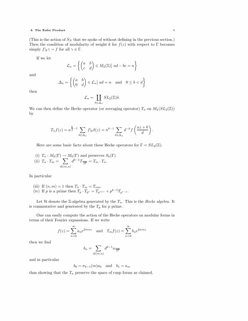
4. The Euler Product 9

(This is the action of SN that we spoke of without defining in the previous section.)Then the condition of modularity of weight k for f(z) with respect to Γ becomessimply f |kγ = f for all γ ∈ Γ.

If we let

Ln =

{(a bc d

)∈M2(Z)

∣∣ ad− bc = n

}

and

∆n =

{(a b0 d

)∈ Ln

∣∣ ad = n and 0 ≤ b < d

}

then

Ln =∐

δ∈∆n

SL2(Z)δ.

We can then define the Hecke operator (or averaging operator) Tn on Mk(SL2(Z))by

Tnf(z) = nk2−1

∑

δ∈∆n

f |kδ(z) = nk−1∑

δ∈∆n

d−kf

(az + b

d

).

Here are some basic facts about these Hecke operators for Γ = SL2(Z).

(i) Tn : Mk(Γ)→Mk(Γ) and preserves Sk(Γ).

(ii) Tn · Tm =∑

d|(m,n)

dk−1Tnm

d2= Tm · Tn.

In particular

(iii) If (n,m) = 1 then Tn · Tm = Tnm.(iv) If p is a prime then Tp · Tpr = Tpr+1 + pk−1Tpr−1 .

Let H denote the Z-algebra generated by the Tn. This is the Hecke algebra. Itis commutative and generated by the Tp for p prime.

One can easily compute the action of the Hecke operators on modular forms interms of their Fourier expansions. If we write

f(z) =

∞∑

n=0

ane2πinz and Tmf(z) =

∞∑

n=0

bne2πinz

then we find

bn =∑

d|(m,n)

dk−1anm

d2

and in particular

b0 = σk−1(m)a0 and b1 = am

thus showing that the Tn preserve the space of cusp forms as claimed.


Suppose now that

f(z) =

∞∑

n=1

ane2πinz

is a cusp form of weight k for SL2(Z) which is a simultaneous eigen-function forall the Hecke operators. If we set Tnf = λ(n)f then we find that the Fouriercoefficients are related to the Hecke eigenvalues by

λ(n)a1 = an

coming from the computation of the first Fourier coefficient of Tnf above. So ifwe normalize f(z) by requiring a1 = 1 then we have λ(n) = an so that the Heckeeigen-values carry the same arithmetic information that the Fourier coefficients do.In addition, from the relations among the Hecke operators, and thus the Heckeeigen-values, we obtain the following recursions on the Fourier coefficients of f .

(i) If (n,m) = 1 then anam = anm.(ii) If p is a prime then apapr = apr+1 + pk−1apr−1 or

apr+1 − apapr + pk−1apr−1 = 0.

If we see what these imply about the L-function associated to f we find

L(s, f) =

∞∑

n=1

anns

=∏

p

(∞∑

r=0

apr

prs

)

=∏

p

(1− app

−s + pk−1p−2s)−1

.

Theorem 1.5 Let f(z) ∈ Sk(SL2(Z)) have a1 = 1. Then f is an eigen-function for all the Hecke operators iff

L(s, f) =∏

p

(1− app

−s + pk−1p−2s)−1

or

Λ(s, f) = (2π)−sΓ(s)∏

p

(1− app

−s + pk−1p−2s)−1

.

5 References

[1] E. Hecke, Uber die Bestimmung Dirischletscher Reihen durch ihre Funktion-algleichung. Math. Ann. 112 (1936), 664–699.

[2] E. Hecke, Mathematische Werke. Vandenhoeck & Ruprecht, Gottingen,1959.

[3] H. Iwaniec, Topics in Classical Automorphic Forms. Graduate Studies inMathematics, 17. American Mathematical Society, Providence, RI, 1997.

[4] G. Shimura, Introduction to the Arithmetic Theory of Automorphic Func-tions. Princeton University Press, Princeton, NJ, 1994.

5. References 11

[5] A. Weil, Uber die Bestimmung Dirichletscher Reihen durch Funktionalgle-ichungen. Math. Ann. 168 (1967), 149–156.

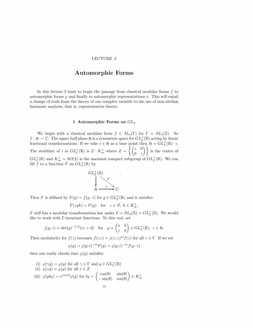
LECTURE 2

Automorphic Forms

In this lecture I want to begin the passage from classical modular forms f toautomorphic forms ϕ and finally to automorphic representations π. This will entaila change of tools from the theory of one complex variable to the use of non-abelianharmonic analysis, that is, representation theory.

1 Automorphic Forms on GL2

We begin with a classical modular form f ∈ Mm(Γ) for Γ = SL2(Z). Sof : H→ C. The upper half plane H is a symmetric space forGL+

2 (R) acting by linearfractional transformations. If we take i ∈ H as a base point then H = GL+

2 (R) · i.

The stabilizer of i in GL+2 (R) is Z · K+

∞ where Z =

{(z 00 z

)}is the center of

GL+2 (R) and K+

∞ = SO(2) is the maximal compact subgroup of GL+2 (R). We can

lift f to a function F on GL+2 (R) by

GL+2 (R)

F

##GGGG

GGGG

G

��H

f // C

.

Then F is defined by F (g) = f(g · i) for g ∈ GL+2 (R) and it satisfies

F (zgk) = F (g) for z ∈ Z, k ∈ K+∞.

F still has a modular transformation law under Γ = SL2(Z) = GL+2 (Z). We would

like to work with Γ-invariant functions. To this end, set

j(g; z) = det(g)−1/2(cz + d) for g =

(a bc d

)∈ GL+

2 (R), z ∈ H.

Then modularity for f(z) becomes f(γz) = j(γ; z)mf(z) for all γ ∈ Γ. If we set

ϕ(g) = j(g; i)−mF (g) = j(g; i)−mf(g · i)

then one easily checks that ϕ(g) satisfies

(i) ϕ(γg) = ϕ(g) for all γ ∈ Γ and g ∈ GL+2 (R)

(ii) ϕ(zg) = ϕ(g) for all z ∈ Z

(iii) ϕ(gkθ) = eπimθϕ(g) for kθ =

(cos(θ) sin(θ)− sin(θ) cos(θ)

)∈ K+

∞

13

14 2. Automorphic Forms

We have interchanged the properties of Γ-modularity and K+∞-invariance for Γ-

invariance and a K+∞-transformation law.

Now let g denote the complexified Lie algebra of GL2(R). Let U(g) denote theuniversal enveloping algebra of g and Z = Z(g) the center of U(g). Z is the spaceof invariant differential operators on GL2(R). Then the holomorphy of f(z) can beexpressed in terms of these operators as

(iv) ϕ(g) is an eigen-function for Z.

Finally, one can express the growth condition of f(z) being holomorphic atinfinity as

(v) ϕ(g) is of moderate growth on GL+2 (R), i.e., for any norm ‖ ‖ on GL+

2 (R)there exists a positive integer r such that

|ϕ(g)| ≤ C‖g‖r.

For the norm we can take ‖g‖ = (tr(gtg) + tr((g−1)tg−1))1/2.

Note that we could do the same passage for a holomorphic modular form forsome Γ0(N) or for a Maass form.

Functions on GL+2 (R) that satisfy (i) – (v) are examples of automorphic forms.

For our purposes it will be more convenient to work with automorphic forms onGL2(A) where A is a ring of adeles. Recall that Q has several completions, namelyR = Q∞ and the various Qp for primes p. The ring of adeles A of Q is then therestricted product of these completions

A = R×∏′

p

Qp =∏′

v

Qv ⊂∏

v

Qv

with respect to the compact open subrings Zp ⊂ Qp. More precisely if we let Sfrun over all finite sets of primes then A is the union, or inductive limit,

A = lim−→Sf

R×

∏

p∈Sf

Qp ×∏

p/∈Sf

Zp

.

Each R×∏p∈Sf

Qp×∏p/∈Sf

Zp receives the product topology and A the inductive

limit topology. Then Q → A diagonally as a canonical discrete subgroup and thequotient Q\A is compact. Note that Z = Q ∩ (R×

∏Zp).

Accordingly, one has

GL2(A) = GL2(R)×∏′

p

GL2(Qp) =∏′

v

GL2(Qv)

= lim−→Sf

GL2(R)×

∏

p∈Sf

GL2(Qp)×∏

p/∈Sf

GL2(Zp)

1. Automorphic Forms on GL2 15

a restricted product with respect to the maximal open compact subgroupsGL2(Zp).Once again GL2(Q) → GL2(A) diagonally as a canonical discrete subgroup havingfinite co-volume modulo the center.

Let us now set G = GL2 and let

G∞ = G(R) ⊃ K = O(2)

Gf =∏′

p

G(Qp) ⊃ Kf =∏

p

Zp

K = K∞Kf ⊂ G∞Gf = G(A).

The groups K∞, Kf and K are all maximal compact subgroups and Kf is open inGf . Then Strong Approximation for SL2 combined with the fact that Q has classnumber one lets us write

G(A) = G(Q) ·G+(R)Kf

and since

Γ = GL+2 (Z) = GL2(Q) ∩ (G+(R)Kf )

we have

Γ\GL+2 (R) = G(Q)\G(A)/Kf

and

Z(R)Γ\GL+2 (R) = Z(A)G(Q)\G(A)/Kf .

To carry out this process for Γ = Γ0(N) we would replace Kf by an appropriateopen compact subgroup L ⊂ Kf which would no longer be maximal.

If we return to our automorphic form ϕ on Z(R)Γ\GL+2 (R) we can further lift

it to a function, still denoted by ϕ, on G(Q)\G(A) by

G(Q)\G(A)

��ϕ

&&LLLLLLLLLLLLLLLLLLLLLLLLLLLL

Z(A)G(Q)\G(A)/Kf

Z(R)Γ\GL+2 (R)

ϕ // C

The function ϕ(g) on G(A) which we construct in this way will be a smoothfunction in the following sense. If we write g ∈ G(A) = G∞ · Gf as g = (g∞, gf )then ϕ(g) = ϕ(g∞, gf ) will be C∞ in the archimedean g∞ variable and locallyconstant in the non-archimedean gf variables. Moreover it will satisfy:

(i) [automorphy] ϕ(γg) = ϕ(g) for all γ ∈ G(Q);(ii) [K-finite] ϕ(gkθkf ) = eimθϕ(g) for kθ ∈ K+

∞ and kf ∈ Kf , or, more gener-ally, the space 〈ϕ(gk) | k ∈ K〉 is finite dimensional;

(iii) [Z-finite] there exists an ideal J ⊂ Z of finite co-dimension such that J ·ϕ =0, or equivalently, the space 〈Xϕ(g) | X ∈ Z〉 is finite dimensional;


(iv) [moderate growth] for any norm ‖ ‖ on G(A) there exists a positive integerr such that

|ϕ(g)| ≤ C‖g‖r.

For an adelic norm on G(A) we can take

‖g‖ =∏

v

(maxi,j{|gi,j|v, |(g

−1)i,j |v}

).

Definition 2.1 A smooth function ϕ : GL2(A) → C satisfying conditions (i)– (iv) is called a (K-finite) automorphic form on GL2(A).

We let A = A(GL2(Q)\GL2(A)) denote the space of automorphic forms onGL2. If we wish to specify a behavior under the center Z(A) then for any continuouscharacter ω : k×\A× → C× we let

A(ω) = {ϕ ∈ A | ϕ(zg) = ω(z)ϕ(g) for z ∈ Z(A)}.

With this generality in the conditions (i)–(iv), the space A will contain the lifts ofall holomorphic modular forms and all Maass forms for all Γ0(N) as well.

2 Automorphic Forms on GLn

It should be clear how to define automorphic forms on GLn(k)\GLn(A) for A

the ring of adeles for any global field k. For our purposes, we will stick to A beingthe ring of adeles of a number field k. Let O denote the ring of integers of k.

The ring A is then the restricted product of the completions kv of k with respectto the maximal compact subrings Ov ⊂ kv for non-archimedean places v <∞.

A =∏′

v

kv = lim−→S

(∏

v∈S

kv ×∏

v/∈S

Ov

)

where now we have taken S to run through all finite sets of places of k such thatS contains V∞ = {v | v|∞}, the set of archimedean places of k. Then we can writeA = k∞Af where

k∞ =∏

v|∞

kv and Af =∏′

v<∞

kv.

If k has r1 real embeddings and r2 pairs of complex embeddings, then k∞ = Rr1 ×Cr2 .

Then

GLn(A) =∏′

v

GLn(kv) = lim−→S

(∏

v∈S

GLn(kv)×∏

v/∈S

GLn(Ov)

)

is the restricted product with respect to the maximal open compact subgroupsKv = GLn(Ov) ⊂ GLn(kv) for the non-archimedean places. If we agree to now letG = GLn then as before we have

G(A) = G∞ ·Gf ⊃ K = K∞ ·Kf

3. Smooth Automorphic Forms 17

where

G∞ = GLn(R)r1 ×GLn(C)r2 ⊃ K∞ = O(n)r1 × U(n)r2

Gf = GLn(Af ) =∏′

v<∞

GLn(kv) ⊃ Kf =∏

v<∞

GLn(Ov).

Again, G(k) → G(A) diagonally as a canonical discrete subgroup with finite co-volume modulo the center Z(A).

Let Z = Z(g) denote the center of the universal enveloping algebra U(g) of thecomplexified Lie algebra g of G∞.

Definition 2.2 A smooth function ϕ : GLn(A) → C is called a (K-finite)automorphic form if it satisfies:

(i) [automorphy] ϕ(γg) = ϕ(g) for all γ ∈ G(Q);(ii) [K-finite] the space 〈ϕ(gk) | k ∈ K〉 is finite dimensional;(iii) [Z-finite] the space 〈Xϕ(g) | X ∈ Z〉 is finite dimensional;(iv) [moderate growth] for any norm ‖ ‖ on G(A) there exists a positive integer

r such that

|ϕ(g)| ≤ C‖g‖r.

We again denote this space by A = A(GLn(k)\GLn(A)).

As in the classical case, the conditions defining automorphic forms imply strongfiniteness results.

Theorem 2.1 (Harish-Chandra) If we fix δ be a finite dimensional repre-sentation of K∞, L ⊂ Kf a compact open subgroup, J ⊂ Z an ideal of finiteco-dimension, and ω : k×\A× → C× a central character and let A(δ, L,J , ω) de-note the set of ϕ ∈ A(ω) such that

(i) ϕ transforms by δ under K∞,(ii) ϕ(gℓ) = ϕ(g) for all ℓ ∈ L,(iii) J · ϕ = 0.

then dimCA(δ, L,J , ω) <∞.

3 Smooth Automorphic Forms

One would hope to be able to analyze A as a representation of GLn(A) actingby right translation. Unfortunately, this is not possible since condition (ii) in thedefinition of automorphic forms is not preserved under right translation. Morespecifically, it is being K∞-finite that is not preserved under right translation byG∞.

[To make this more precise, consider ϕ(g) ∈ A and set

ϕ′(g) = R(g′)ϕ(g) = ϕ(gg′).


Then ϕ(g) is right K-finite and ϕ′(g) is naturally right K ′-finite where K ′ =g′K(g′)−1 is a conjugate of K. Now, at the finite places, since Kf and K ′

f are

both compact and open, the intersection Kf ∩ K ′f is of finite index in both. So

there is no difference between Kf -finiteness and K ′f -finiteness. On the other hand

at the archimedean places there is no reason for K∞ and K ′∞ to have anything

more in common than the identity. This is quite apparent when considering GL2

or SL2 where the maximal compacts are one dimensional. So while the notion ofbeing Kf -finite is really independent of the choice of maximal compact, the notionof K∞-finiteness is dependent on the choice of K∞.]

There are two ways to remedy this: (i) settle for representations of somethingsmaller – namely the Hecke algebra H; or (ii) enlarge the space of automorphicforms. We will address the Hecke algebra in the next lecture. The most naturalenlargement is the space of smooth automorphic forms, in which the condition ofK∞-finiteness is weakened to a condition of uniform moderate growth.

Definition 2.3 A smooth function ϕ : GLn(A) → C is called a smooth auto-morphic form if it satisfies:

(i) [automorphy] ϕ(γg) = ϕ(g) for all γ ∈ G(Q);(ii) [Kf -finite] there is a compact open subgroup L ⊂ Kf such that ϕ(gℓ) = ϕ(g)

for all ℓ ∈ L;(iii) [Z-finite] there exists an ideal J ⊂ Z of finite co-dimension such that Jϕ =

0;(iv) [uniform moderate growth] there exists a positive integer r such that for all

differential operators X ∈ U(g)

|Xϕ(g)| ≤ CX‖g‖r.

We will denote the space of smooth automorphic forms by

A∞ = A∞(GLn(k)\GLn(A)).

Now GLn(A) does act on A∞ by right translation. Moreover A∞ will carry a limitFrechet topology coming from the uniform moderate growth semi-norms. A∞ isnot that far removed from A. By a theorem of Harish-Chandra we know that K∞-finiteness implies uniform moderate growth, so that A ⊂ A∞ and A is preciselythe space of ϕ ∈ A∞ that are K-finite, and that in fact A is dense in A∞ in thisnatural topology.

4 L2-automorphic Forms

Another natural class of automorphic forms are the L2-automorphic forms. Todefine these we must fix a unitary central character ω : k×\A× → C1. Then

L2(ω) = L2(GLn(k)\GLn(A);ω)

is the space of all measurable ϕ : GLn(k)\GLn(A)→ C such that ϕ(zg) = ω(z)ϕ(g)for z ∈ Z(A) and ∫

Z(A)GLn(k)\GLn(A)

|ϕ(g)|2 dg <∞.

5. Cusp Forms 19

This is a Hilbert space and the group GLn(A) acts by right translation on this spacepreserving the norm; hence L2(ω) affords a unitary representation of GLn(A).

5 Cusp Forms

As in the classical case, the cusp forms will play a special role for us. Recallthat if f(z) is a classical modular form for Γ = SL2(Z) then f is a cusp form if

0 = a0 =

∫ 1

0

f(x+ iy) dx =

∫ 1

0

f

((1 x0 1

)· iy

)dx.

If ϕ(g) is an automorphic form on GL2, then the group of translations is

N2 =

{n =

(1 x0 1

)}⊂ GL2.

The analogous integral would be overN2(k)\N2(A) ≃ k\A, which is compact. Thuswe have the following definition.

Definition 2.4 An automorphic form ϕ(g) on GL2(A) is a cusp form iff∫

N2(k)\N2(A)

ϕ(ng) dn =

∫

k\A

ϕ

((1 x0 1

)g

)dx = 0.

This is the same no matter whether ϕ ∈ A, A∞, or L2.

For GLn there are many translation subgroups. They are given by the unipo-tent radicals of (rational) parabolic subgroups. For GLn the parabolic subgroupsare parameterized (up to conjugation) by partitions n = n1 + · · · + nr of n. Theassociated parabolic is

P =

g1 ∗ · · · ∗0 g2 · · · ∗...

. . ....

0 · · · · · · gr

∣∣gi ∈ GLni

= M · U

where M ≃ GLn1 × · · · ×GLnris the Levi subgroup and

U =

In1 ∗ · · · ∗0 In2 · · · ∗...

. . ....

0 · · · · · · Inr

is the unipotent radical of P . P is called proper if the partition is non-trivial. Asfor GL2 for any of these unipotent radicals, U(k)\U(A) is compact.

Definition 2.5 An automorphic form ϕ(g) on GLn(A) is a cusp form iff∫

U(k)\U(A)

ϕ(ug) du = 0

for all unipotent radicals of all proper parabolic subgroups of GLn.


Since all parabolics are (rationally) conjugate to a standard (upper triangular)one, it suffices to only consider integrals over the standard unipotent radicals. (Thisis often referred to by saying that when one works adelically GLn has only onecusp.) In fact, it suffices to consider only unipotent radicals of maximal parabolicsubgroups, i.e., those associated to partitions with only two terms n = n1 + n2, so

P =

{(g1 X

g2

)}⊃ U =

{(In1 X

In2

)}≃Mn1×n2 ,

since at least one of these unipotent groups will occur as a normal subgroup in anyother standard unipotent radical.

As in the classical case we have that cusp forms are rapidly decreasing.

Theorem 2.2 (Gelfand and Piatetski-Shapiro) If ϕ(g) is a cusp form,then it is rapidly decreasing modulo the center on a fundamental domain F forGLn(k)\GLn(A), that is, for some integer r

|g(zg)| ≤ C|z|r‖g‖−N for all N ∈ N

where we restrict g to lie in F ∩ SLn(A).

We should note that exact fundamental domains for GLn(A) are rather un-wieldy and instead one usually replaces F with a slightly bigger set S, called aSiegel set, which is easier to construct.

We will denote the subspaces of cusp forms by A0, A∞0 , and L2

0. Note that ifwe fix a unitary central character ω then one consequence of this rapid decay is thecontainment A0(ω) ⊂ A∞

0 (ω) ⊂ L20(ω).

6 References

[1] A. Borel and H. Jacquet, Automorphic forms and automorphic representa-tions. Proc. Sympos. Pure Math. 33, part 1, (1979), 189–207.

[2] S. Gelbart, Automorphic Forms on Adele Groups. Annals of Math. Studies83, Princeton University Press, Princeton, 1975.

[3] I.M. Gelfand, M.I. Graev, and I.I. Piatetski-Shapiro, Representation Theoryand Automorphic Functions. Saunders, Philadelphia, 1968.

[4] Harish-Chandra, Automorphic forms on Semisimple Lie Groups. LectureNotes in Mathematics, No. 62 Springer-Verlag, Berlin-New York 1968.

[5] N.R. Wallach, C∞ vectors. Representations of Lie Groups and QuantumGroups, Pitman Res. Notes Math. Ser. 311, Longman Sci. Tech., Harlow, 1994,205–270.

LECTURE 3

Automorphic Representations

We have defined our spaces of automorphic forms. Now we turn to our tools.We will analyze A, A∞, or L2(ω) as representation spaces for certain algebras orgroups. Throughout we will let G = GLn, although the results remain true for anyreductive algebraic group G, let k be a number field, and retain all notations frombefore.

1 (K-finite) automorphic representations

As we have noted the space A of (K-finite) automorphic forms does not givea representation of G(A). It will be a representation space for the global Heckealgebra H.

1.0.1 The Hecke algebra. The global Hecke algebraH will be a restricted tensorproduct of local Hecke algebras: H = ⊗′Hv. H and each Hv will be idempotentedalgebras under convolution. So there will be a directed family of fundamentalidempotents {ξi} such that

H = lim−→i

ξi ∗ H ∗ ξi =⋃

i

ξi ∗ H ∗ ξi

andHv = lim

−→i

ξi,v ∗ Hv ∗ ξi,v =⋃

i

ξi,v ∗ H ∗ ξi,v.

Neither H nor any Hv will have an identity, but for each ξi the subalgebra ξi ∗H∗ξiwill have ξi as an identity.

(i) If v < ∞ is an non-archimedean place of k then Hv = C∞c (G(kv)) is the

algebra of smooth (locally compact) compactly supported functions on Gv = G(kv).It is naturally an algebra under convolution. For each compact open subgroupLv ⊂ Gv there is a fundamental idempotent

ξLv=

1

V ol(Lv)XLv

where XLvis the characteristic function of Lv. Then ξLv

∗ Hv ∗ ξLv= H(Gv//Lv)

is the algebra of Lv-bi-invariant compactly supported functions on Gv. In anyrepresentation of Hv the idempotent ξLv

will act as a projection onto the Lv-fixed vectors. We will let ξ◦v denote the fundamental idempotent associated to themaximal compact subgroup Kv. Note that if k = Q, G = GL2, and Lp = Kp =GL2(Zp) then ξ◦p ∗Hp ∗ ξ

◦p = H(GL2(Qp)//GL2(Zp)) is isomorphic to the complex

algebra spanned by the classical Hecke operators 〈Tpr 〉.

21

22 3. Automorphic Representations

(ii) If v|∞ is an archimedean place of k then Hv is the convolution algebra ofbi-Kv-finite distributions on Gv with support in Kv. Then Hv contains both

U(g) : distributions supported at the identity

and

A(Kv) : finite measures on Kv

and in fact

Hv = U(gv)⊗U(kv) A(Kv).

For each finite dimensional representation δv of Kv we have a fundamental idem-potent

ξδv=

1

deg(δv)Θδv

dkv

where deg(δv) is the degree and Θδvis the character of δv and dkv is the normalized

Haar measure on Kv . In any representation δv should act as the projection ontothe δv-isotypic component.

(iii) The global Hecke algebra H is then the restricted tensor product of thelocal algebras Hv with respect to the idempotents {ξ◦v} at the non-archimedeanplaces., i.e.,

H = ⊗′vHv = lim

−→S

((⊗v∈SHv)⊗ (⊗v/∈Sξ◦v ))

as S runs over finite sets of places of k which contain all archimedean places V∞.Let us write H = H∞ ⊗Hf where, as usual,

H∞ = ⊗v|∞Hv and Hf = ⊗′v<∞Hv.

Then the fundamental idempotents in H are of the form ξ = ξ∞ ⊗ ξf where

ξ∞ = ξδ = ⊗v|∞ξδv∈ H∞

is associated to a finite dimensional representation δ = ⊗δv of K∞ and

ξf = ξL = ⊗v<∞ξLv∈ Hf

is associated to a compact open subgroup L =∏Lv of Gf (so for almost all places

Lv = Kv and ξLv= ξ◦v).

1.0.2 The representation on automorphic forms. The space A of K-finite au-tomorphic forms is naturally an H-module by right convolution. For ξ ∈ H andϕ ∈ A set

R(ξ)ϕ(g) = ϕ ∗ ξ(g) =

∫

G(A)

ϕ(gh)ξ(h) dh

where ξ(g) = ξ(g−1). Note that with this action the K-finiteness condition onϕ ∈ A can now be stated as: there exists a fundamental idempotent ξ = ξ∞⊗ ξf =ξδ ⊗ ξL such that R(ξ)ϕ = ϕ.

The representations that we will be most interested in will be admissible rep-resentations of H.

Definition 3.1 A representation (πv, Vv) of a local Hecke algebra Hv is ad-missible if for every fundamental idempotent ξv we have

dimC(πv(ξv)Vv) <∞.

1. (K-finite) automorphic representations 23

Similarly a representation (π, V ) of the global Hecke algebra H is admissible if forevery global fundamental idempotent ξ ∈ H the subspace π(ξ)V is finite dimen-sional.

One consequence of admissibility, which we state in the global case, is that as arepresentation of K the space V decomposes into a direct sum of irreducibles withfinite multiplicities:

V =⊕

τ∈K

m(τ, V )Vτ .

The reason for our interest in admissible representations is the following fun-damental result of Harish-Chandra (probably first due to Jacquet and Langlandsfor GL2).

Theorem 3.1 Suppose ϕ ∈ A. Then the H-module generated by ϕ, namely

Vϕ = R(H)ϕ = ϕ ∗ H ⊂ A,

is an admissible H-module.

This makes the following definition reasonable.

Definition 3.2 An automorphic representation (π, V ) of H is an irreducible(hence admissible) sub-quotient of A(G(k)\G(A)).

There is a canonical way to construct admissible representations ofH abstractlyusing the restricted tensor product structure H = ⊗′Hv. Suppose we have a col-lection {(πv, Vv)} of admissible representations of the local Hecke algebras Hv suchthat for almost all finite places the representation Vv contains a (fixed) Kv-invariantvector, say u◦v. Then we can define the restricted tensor product of these represen-tations with respect to the {u◦v} in the (by now) usual manner:

V = ⊗′vVv = lim−→

S

((⊗v∈SVv)⊗ (⊗v/∈Su◦v)) .

Note that since u◦v isKv-fixed, then πv(ξ◦v )u

◦v = u◦v so this space does carry a natural

representation ofH, coming from its restricted tensor product decomposition, whichwe will denote by π = ⊗′πv. We leave it as an exercise to verify that if each of the(πv, Vv) is admissible then so is (π, V ) and if each (πv, Vv) is irreducible, then so is(π, V ).

An important fact for us, which is a purely algebraic fact about H-modules, isthe converse to this construction.

Theorem 3.2 (Decomposition Theorem) If (π, V ) is an irreducible ad-missible representation of H then for each place v of k there exists an irreducibleadmissible representation (πv, Vv) of Hv, having a Kv-fixed vector for almost all v,such that π = ⊗′πv.

Therefore in the context of automorphic representations of H we have thefollowing corollary.


Corollary 3.2.1 If (π, V ) is an automorphic representation, then π decom-poses into a restricted tensor product of local irreducible admissible representations:π = ⊗′πv.

Note that the decomposition given in this corollary is an abstract decompo-sition. It does not give a factorization of automorphic forms into a product offunctions on the local groups G(kv).

2 Smooth automorphic representations

Now things are more straight forward on the one hand, since G(A) acts inA∞(G(k)\G(A)) by right translation. However the representation theory is now abit more complicated. More precisely, for every compact open subgroup L ⊂ Kf

the space of L-invariant functions (A∞)L in A∞, namely

(A∞)L = {ϕ ∈ A∞ | ϕ(gℓ) = ϕ(g) for ℓ ∈ L},

is a representation for G∞. The spaces (A∞)L all carry compatible limits of smoothFrechet topologies coming from the uniform moderate growth semi-norms on A∞

and the representation of G∞ on these spaces are limits of smooth Frechet repre-sentation of moderate growth. More precisely, if we let

A∞r = {ϕ ∈ A∞ | sup

g∈G(A)

(‖g‖−r|Xϕ(g)|) <∞ for all X ∈ U(g)}

then for any open compact subgroup L ⊂ Kf the space of L-fixed vectors (A∞r )L

in A∞r is a smooth Frechet representation of moderate growth for G∞ defined by

the natural seminorms

qX,r(ϕ) = supg

(‖g‖−r|Xϕ(g)|) for X ∈ U(g).

Then as topological representations both

(A∞)L = lim−→r

(A∞r )L and A∞ = lim

−→L

(A∞)L

carry a limit-Frechet topology. Without going into details on such representations,let us state the results we will need analogous to those for representations of H.

Theorem 3.3 (Harish-Chandra; Wallach) If ϕ ∈ A∞ is a smooth auto-morphic form then the (closed) sub-representation generated by ϕ, namely

Vϕ = R(G(A))ϕ ⊂ A∞,

is admissible in the sense that its (dense) subspace of K-finite vectors (Vϕ)K isadmissible as an H-module.

Then we can make the following definition.

Definition 3.3 A smooth automorphic representation (π, V ) of G(A) is a(closed) irreducible sub-quotient of A∞(G(k)\G(A)).

Note that the smooth automorphic representations are automatically admis-sible in the above sense. We still have a version of the Decomposition Theorem,which we state as follows.

3. L2-automorphic representations 25

Theorem 3.4 (Decomposition Theorem) If (π, V ) is a smooth automor-phic representation of G(A) then there exist irreducible admissible smooth repre-sentations (πv, Vv) of G(kv), which are smooth Frechet representations of moderategrowth if v|∞, such that π = π∞ ⊗ πf where

π∞ = ⊗v|∞πv

is the topological tensor product of smooth Frechet representations and

πf = ⊗′v<∞πv

is the restricted tensor product of smooth representations of the G(kv). Moreover, if(πK , VK) is the associated irreducible H-module of K-finite vectors in V then in thedecomposition πK = ⊗′(πK)v we have πv = (πK)v for v <∞ while for v|∞ we have

(πv)K = (πK)v and πv = (πK)v is the Casselman-Wallach canonical completion ofthe Hv-module (πK)v.

Even though the theory of smooth automorphic representations is topological,according to Wallach it is also quite algebraic. These representations will be alge-braically irreducible as representations of the global Schwartz algebra S = S(G(A)).This is a restricted tensor product of the local Schwatrz algebras Sv = S(G(kv)).For archimedean places v|∞ then Sv is the usual space of smooth (infinitely dif-ferentiable) rapidly decreasing functions on G(kv). At the non-archmiedean placesrapidly decreasing is interpreted as having compact support, so Sv is the space ofsmooth (locally constant) compactly supported supported functions on G(kv), thatis, Sv = Hv. Then S = S∞ ⊗ Sf where now

S∞ = S(G∞) = ⊗v|∞Sv and Sf = ⊗′v<∞Sv = Hf .

3 L2-automorphic representations

If we now fix a unitary central character ω : k×\A× → C× and consider theassociated space of L2-automorphic forms L2(G(k)\G(A);ω) then this space is aHilbert space and affords a unitary representation representation of G(A) acting byright translation. In some sense this is the easiest situation to be in.

Theorem 3.5 (Harish-Chandra) If ϕ ∈ L2(ω) then

Vϕ = R(G(A))ϕ ⊂ L2(ω)

is an admissible sub-representation in the sense that the (dense) sub-space (Vϕ)Kof K-finite vectors is admissible as as H-module.

Definition 3.4 An L2-automorphic representation (π, V ) is an irreducible con-stituent in the L2-decomposition of some L2(ω).

In the context of L2-automorphic representations, the Decomposition Theorempredates the algebraic one and is due to Gelfand and Piatetski-Shapiro.

Theorem 3.6 If (π, V ) is an L2-automorphic representation then there ex-

ist irreducible unitary representations (πv, Vv) of G(kv) such that π = ⊗′πv is a

restricted Hilbert tensor product of local representations.


4 Cuspidal representations

Since the cuspidality condition is defined by the vanishing of a left unipotentintegration ∫

U(k)\U(A)

ϕ(ug) du = 0,

which is a closed condition, and our actions of H or G(A) on the spaces of auto-morphic forms are by right convolution or right translations we see that the spacesof cusp forms A0, A∞

0 , or L20(ω) are all (closed) sub-representations of the relevant

spaces of automorphic forms.

A fundamental result of the space of L2-cusp forms is the following result ofGelfand and Piatetski-Shapiro.

Theorem 3.7 The space L20(ω) of L2-cusp forms decomposes into a discrete

Hilbert direct sum with finite multiplicities of irreducible unitary sub-representations

L20(ω) = ⊕m(π)Vπ with m(π) <∞.

We can then make the following definition.

Definition 3.5 The irreducible constituents (π, Vπ) of the various L20(ω) are

the L2-cuspidal representations.

Recall that for a fixed unitary central character ω we have, as a consequenceof the rapid decrease of cusp forms, the inclusions

A0(ω) ⊂ A∞0 (ω) ⊂ L2

0(ω)

and in fact upon passing to smooth vectors and then K-finite vectors we have

A∞0 (ω) = L2

0(ω)∞ and A0(ω) = A∞0 (ω)K = L2

0(ω)K

so we can deduce the decompositions

A∞0 (ω) = ⊕m(π)V∞

π and A0(ω) = ⊕m(π)(Vπ)K .

Definition 3.6 The irreducible constituents of A0(ω) are the unitary (K-finite)cuspidal representations of G(A) and the irreducible constituents of A∞(ω) are theunitary smooth cuspidal representations of G(A).

Note that if (π, Vπ) is a cuspidal representation (in any context) then the el-ements of Vπ are indeed cusp forms, that is, Vπ ⊂ A0 as a subspace not a moregeneral sub-quotient.

In general any irreducible subrepresentation of A0 or A∞0 will be called a cuspi-

dal representation. Due to the rapid decrease of cusp forms, any cuspidal represen-tation (π, Vπ) will be an unramified twist of a unitary cuspidal representation, thatis, if we define for any character χ : k×\A× → C× the twisted representation π⊗χas the representation by right translation on the space V ⊗ χ = {ϕ(g)χ(det g) |ϕ ∈ Vπ}, then one can always find an unramified character χ such that π ⊗ χ isa unitary cuspidal representation as above. Some choose to call the non-unitarycuspidal representations quasi-cuspidal.

6. References 27

5 Connections with classical forms

Suppose we return to a classical cusp form f for SL2(Z) of weight m. If wefollow our passage f 7→ ϕ 7→ (πϕ, Vϕ) then (πϕ, Vϕ) is an admissible subspace ofthe space of cuspidal automorphic forms. It need not be irreducible. However, if inaddition f is a simultaneous eigen-function for all the classical Hecke operators, then(πϕ, Vϕ) is irreducible and hence a cuspidal representation. Then the DecompositionTheorem lets us decompose πϕ as πϕ = π∞ ⊗ (⊗′πp). In this decomposition

(i) π∞ is completely determined by the weight m of f(ii) πp is completely determined by the Hecke eigen-value λ(p) of Tp acting on

f .

In fact, as we shall see, the Decomposition Theorem for πϕ is equivalent to theEuler product factorization for the completed L-function Λ(s, f).

6 References

[1] A. Borel and H. Jacquet, Automorphic forms and automorphic representa-tions. Proc. Sympos. Pure Math. 33, part 1, (1979), 189–207.

[2] D. Flath, Decomposition of representations into tensor products. Proc. Sym-pos. Pure Math. 33, part 1, (1979), 179–183.

[3] I.M. Gelfand, M.I. Graev, and I.I. Piatetski-Shapiro, Representation Theoryand Automorphic Functions. Saunders, Philadelphia, 1968.

[4] Harish-Chandra, Automorphic forms on Semisimple Lie Groups. LectureNotes in Mathematics, No. 62 Springer-Verlag, Berlin-New York 1968.

[5] H. Jacquet and R.P. Langlands, Automorphic Forms on GL(2). SpringerLecture Notes in Mathematics, No. 114, Springer-Verlag, Berlin-New York, 1971.

[6] N.R. Wallach, C∞ vectors. Representations of Lie Groups and QuantumGroups, Pitman Res. Notes Math. Ser. 311, Longman Sci. Tech., Harlow, 1994,205–270.

LECTURE 4

Fourier Expansions and Multiplicity One

Theorems

We now start with results which are often GLn specific. So we let G = GLn(however one should also keep in mind G = GLn ×GLm) and still take k to be anumber field.

1 The Fourier expansion of a cusp form

Let (π, Vπ) be a smooth cuspidal representation, so Vπ ⊂ A∞0 . Let ϕ ∈ Vπ be

a smooth cusp form.

We begin with G = GL2. Our translation subgroup is

N = N2 =

{n =

(1 x0 1

)}.

For any g ∈ G(A) the function

x 7→ ϕ

((1 x0 1

)g

)

is a smooth function of x ∈ A which is periodic under k. Since k\A is a compactabelian group we will have an abelian Fourier expansion of this function.

For each continuous character ψ : k\A → C we define a ψ-Fourier coefficient,or ψ-Whittaker function, of ϕ by

Wϕ,ψ(g) =

∫

k\A

ϕ

((1 x0 1

)g

)ψ−1(x) dx.

This function satisfies

Wϕ,ψ

((1 x0 1

)g

)= ψ(x)Wϕ,ψ(g).

Then by standard abelian Fourier analysis we have

ϕ

((1 x0 1

)g

)=∑

ψ∈dk\A

Wϕ,ψ(g)ψ(x)

or

ϕ(g) =∑

ψ

Wϕ,ψ(g).

29

30 4. Fourier Expansions and Multiplicity One Theorems

By standard duality theory, k\A ≃ k and if we fix one non-trivial character ψ thenany other is of the form ψγ(x) = ψ(γx) for γ ∈ k, so

ϕ(g) =∑

γ∈k

Wϕ,ψγ(g).

Since ϕ is cuspidal, for γ = 0 we have

Wϕ,ψ0(g) =

∫

k\A

ϕ

((1 x0 1

))dx = 0

and for γ 6= 0 it is an easy change of variables to see that

Wϕ,ψγ(g) = Wϕ,ψ

((γ 00 1

)g

)

which gives for our Fourier expansion for GL2

ϕ(g) =∑

γ∈k×

Wϕ

((γ 00 1

)g

)

where we have set Wϕ,ψ = Wϕ.

Now consider G = GLn. The role of the translations is played by the fullmaximal unipotent subgroup

N = Nn =

n =

1 x1,2 ∗. . .

. . .

. . . xn−1,n

0 1

which is now non-abelian. If we retain out fixed additive character ψ of k\A frombefore, then ψ defines a (continuous) character of N(k)\N(A) by

ψ(n) = ψ

1 x1,2 ∗. . .

. . .

. . . xn−1,n

0 1

= ψ(x1,2 + · · ·+ xn−1,n).

The associated ψ-Whittaker function of ϕ is now

Wϕ(g) = Wϕ,ψ(g) =

∫

N(k)\N(A)

ϕ(ng)ψ−1(n) dn

which again satisfiesWϕ(ng) = ψ(n)Wϕ(g) for all n ∈ N(A). The Fourier expansionof ϕ which is useful is

ϕ(g) =∑

γ∈Nn−1(k)\GLn−1(k)

Wϕ

((γ 00 1

)g

).

This is not hard to prove. It is essentially an induction based on the aboveargument, begun by expanding about the last column of N , which is abelian.

2. Whittaker models 31

For G = GL3 one would begin with

ϕ

1 x1 x2

1 x3

1

g

= ϕ

1 x2

1 x3

1

1 x1

11

g

and expand this as a function of

(x2

x3

)∈ (k\A)2. Remember that ((k\A)2)∧ ≃ k2

and that GL2(k) acts on k2 with two orbits: {0} and an open orbit (0, 1) ·GL2(k).The {0} orbit contributes 0 by cuspidality and the open orbit can be parameterized

by P2(k)\GL2(k) where P2 =

{(a b0 1

)}= Stab((0, 1)). One then expands the

resulting terms as functions of x1 as before.

As I said, the proof is not hard. The difficult thing, if there is one, is inrecognizing that this is what one needs. This was recognized independently byPiatetski-Shapiro and Shalika.

2 Whittaker models

Consider now the functions W = Wϕ which appear in the Fourier expansion ofour cusp forms ϕ ∈ Vπ . These are smooth functions on G(A) satisfying W (ng) =ψ(n)W (g) for all n ∈ N(A). Let

W(π, ψ) = {Wϕ | ϕ ∈ Vπ}.

The group G(A) acts in this space by right translation and the map

ϕ 7→Wϕ intertwines Vπ∼−→W(π, ψ).

Note that since we can recover ϕ from Wϕ through its Fourier expansion we areguaranteed that Wϕ 6= 0 for all ϕ 6= 0. The space W(π, ψ) is called the Whittakermodel of π.

The idea of a Whittaker model makes sense over a local field (and even a finitefield). If we let kv be a local field (a completion of our global field k) and let ψvbe a non-trivial (continuous) additive character of kv then as before ψv defines acharacter of the local translationsN(kv). LetW(ψv) denote the full space of smoothfunctions W : G(kv) → C which satisfy W (ng) = ψv(n)W (g) for all n ∈ N(kv).This is the space of smooth Whittaker functions on G(kv) and G(kv) acts on it byright translation.

If (πv, Vπv) is a smooth irreducible admissible representation of G(kv), then an

intertwining

Vπv→ W(ψv) given by ξv 7→Wξv

gives a Whittaker model W(πv, ψv) of πv.

For a representation (πv, Vπv) to have a Whittaker model it is necessary and

sufficient for Vπvto have a non-trivial (continuous) Whittaker functional, that is ,

a continuous functional Λv : Vπv→ C satisfying

Λv(πv(n)ξv) = ψv(n)Λv(ξv)


for all n ∈ N(kv) and ξv ∈ Vπv. A model ξv 7→Wξv

gives a functional by

Λv(ξv) = Wξv(e)

and a functional Λv gives a model by setting

Wξv(g) = Λv(πv(g)ξv).

The fundamental result on local Whittaker models is due to Gelfand and Kazh-dan (v <∞) and Shalika (v|∞).

Theorem 4.1 (Local Uniqueness) Given (πv, Vπv) an irreducible admissible

smooth representation of G(kv) the space of (continuous) Whittaker functionals isat most one dimensional, that is, and πv has at most one Whittaker model.

Remarks. (i) One proves this by showing that the space of Whittaker functionsW(ψv) is multiplicity free as a representation ofG(kv). WritingW(ψv) = Ind(ψv)

∞

one shows that the intertwining algebra of Bessel distributions, that is, distributionsB satisfying B(n1gn2) = ψv(n1)B(g)ψv(n2), is commutative by exhibiting an anti-involution of the algebra that stabilizes the individual distributions.(ii) When v|∞, if we worked simply with irreducible admissible representationsof the Hecke algebra Hv then the space of (algebraic) Whittaker functionals on(Vπv

)K would have dimension n!, but only one extends continuously to Vπvwith

its (smooth moderate growth) Frechet topology.(iii) Simultaneously, one shows that if πv has a Whittaker model, then so does itscontragredient πv and in fact

W(πv, ψ−1v ) = {W (g) = W (wn

tg−1) |W ∈ W(πv, ψv)}

where wn denotes the long Weyl element wn =

1. .

.

1

.

Definition 4.1 A representation (πv, Vπv) having a Whittaker model is called

generic.

Of course, the same definition applies in the global situation. Note that forG = GLn this notion is independent of the choice of (non-trivial) ψv or ψ.

Now return to our smooth cuspidal representation (π, Vπ), or in fact any ir-reducible admissible smooth representation of G(A). If we factor π into its localcomponents

π ≃ ⊗′πv with Vπ ≃ ⊗′Vπv

then any Whittaker functional Λ on Vπ determines a family of compatible Whittakerfunctionals Λv on the Vπv

by

Λv : Vπv→ ⊗′Vπv

∼−→ Vπ

Λ−→ C

such that Λ = ⊗Λv. Similarly, any suitable family {Λv} of Whittaker functionalson the Vπv

, where suitable means Λv(ξ◦v ) = 1 for our distinguished Kv-fixed vectors

ξ◦v giving the restricted tensor product, determines a global Whittaker functionalΛ = ⊗Λv on Vπ = ⊗′Vπv

.

The Local Uniqueness Theorem then has the following consequences.

3. Multiplicity One for GLn 33

Corollary 4.1.1 (Global Uniqueness) If π = ⊗′πv is any irreducible ad-missible smooth representation of G(A) then the space of Whittaker functionals ofVπ is at most one dimensional, that is, π has a unique Whittaker model.

If (π, Vπ) is our cuspidal representation then we have seen that Vπ has a globalWhittaker functional given by

Λ(ϕ) = Wϕ(e) =

∫

N(k)\N(A)

ϕ(n)ψ−1(n) dn.

Corollary 4.1.2 If (π, Vπ) is cuspidal with π ≃ ⊗′πv then π and each of itslocal components πv are generic.

A most important consequence for our purposes is:

Corollary 4.1.3 (Factorization of Whittaker Functions) If (π, Vπ) is acuspidal representation with π ≃ ⊗′πv and ϕ ∈ Vπ such that under the isomorphismVπ ≃ ⊗

′Vπvwe have ϕ 7→ ⊗ξv (so ϕ is decomposable) then

Wϕ(g) =∏

v

Wξv(gv).

The proof is essentially the following simple computation:

Wϕ(g) = Λ(π(g)ϕ) = (⊗Λv)(⊗πv(gv)ξv)

=∏

v

Λv(πv(gv)ξv) =∏

v

Wξv(gv).

Note once again that the cusp form ϕ(g) itself does not factor. The G(k)-invariance mixes the various places together. Only Wϕ factors for decomposable ϕ.If f ∈ Sm(SL2(Z)) is a classical Hecke eigen-form of weight m for SL2(Z), with itsusual Fourier expansion f(z) =

∑ane

2πinz, and f 7→ ϕ is our lifted automorphicform, then ϕ is decomposable and the Whittaker function Wϕ factors. If we writeWϕ = W∞Wf then

W∞

(ny

1

)= (ny)m/2e−2πny and Wf

(n

1

)= an.

3 Multiplicity One for GLn

The uniqueness of the Whittaker model is the key to the following result.

Theorem 4.2 (Multiplicity One) Let (π, Vπ) be a smooth irreducible admis-sible (unitary) representation of GLn(A). Then its multiplicity m(π) in the spaceof cusp forms is at most one.

This result was proven independently by Piatetski-Shapiro and Shalika, basedon the Fourier expansion and the global uniqueness of Whittaker models. Supposewe have two realizations of π in the space of cusp forms:

Vπ → Vπ,i ⊂ A∞0 for i = 1, 2.


For ξ ∈ Vπ let ϕ1 and ϕ2 be the corresponding cusp forms. Then the maps

ξ 7→ ϕi 7→Wϕi(e) = Λi(ξ)

give two Whittaker functionals on Vπ . By uniqueness, there exists c 6= 0 such thatΛ1 = cΛ2. Then

Wϕ1(g) = Λ1(π(g)ξ) = cΛ2(π(g)ξ) = cWϕ2(g)

so that

ϕ1(g) =∑

γ

Wϕ1

((γ 00 1

)g

)= c

∑

γ

Wϕ2

((γ 00 1

)g

)= cϕ2(g).

But then Vπ,1 ∩ Vπ,2 6= {0}. So by irreducibility Vπ,1 = Vπ,2, that is, m(π) = 1.

4 Strong Multiplicity One for GLn

Strong Multiplicity One was originally due to Piatetski-Shapiro. His proof,which we will sketch here, is a variant of the proof of Multiplicity One. We willgive a second proof due to Jacquet and Shalika based on L-functions later.

Theorem 4.3 (Strong Multiplicity One) Let (π1, Vπ1) and (π2, Vπ2) betwo cuspidal representations of GLn(A). Decompose them as π1 ≃ ⊗′π1,v andπ1 ≃ ⊗′π2,v. Suppose that there is a finite set of places S such that π1,v ≃ π2,v forall v /∈ S. Then (π1, Vπ1) = (π2, Vπ2).

In place of the Whittaker model, Piatetski-Shapiro used a variant known as theKirillov model. To define this, let

P = Pn =

∗ · · · ∗ ∗...

......

∗ · · · ∗ ∗0 · · · 0 1

= Stab ((0, . . . , 0, 1))

denote the mirabolic subgroup of GLn. If we let (πv, Vπv) be an irreducible admis-

sible generic representation of G(kv) with Whittaker model W(πv, ψv) then we canconsider the restrictions Wv(pv) of the functions Wv ∈ W(πv, ψv) to Pv = P (kv).The first surprising fact is:

Theorem 4.4 The map Wv 7→ Wv|Pvis injective, that is, if Wv 6= 0 then

Wv(pv) 6≡ 0.

This is due to Bernstein and Zelevinsky if v < ∞ and Jacquet and Shalika ifv|∞.

Definition 4.2 The (local) Kirillov model of a generic (πv, Vπv) is the space

of functions on Pv defined by

K(πv, ψv) = {Wv(pv) |Wv ∈ W(πv, ψv), pv ∈ Pv}.

5. References 35

A second surprising fact is that no matter what the generic representation(πv, Vπv

) we begin with, the Kirillov models all have a common Pv sub-module,namely

τ(ψv) =

indPv

Nv(ψv) v <∞

IndPv

Nv(ψv)

∞ v|∞

.

This is a canonical space of functions on Pv. The result for v <∞ is of course dueto Bernstein and Zelevinsky and for v|∞ it is due to Jacquet and Shalika.

We may now sketch the proof of the Strong Multiplicity One Theorem. Let π1,π2, and S be as in the statement of the theorem. As before, our goal is to producea common non-zero cusp form ϕ ∈ Vπ1 ∩ Vπ2 .

(i) Let P ′ = P ′n = PnZn be the (n− 1, 1) parabolic subgroup of GLn (here Zn

is still the center of GLn). Then P ′(k)\P ′(A) is dense in GLn(k)\GLn(A). [Thisfollows from the fact that P ′\GLn ≃ Pn−1 and Pn−1(k) is dense in Pn−1(A).] Soit suffices to find ϕi ∈ Vπi

such that ϕ1(p′) = ϕ2(p

′) for all p′ ∈ P ′(A).

(ii) Utilizing the Fourier expansion as before, it suffices to find non-zero Wi ∈W(πi, ψ) such that W1(p

′) = W2(p′).

(iii) Since ω = ωπ1 = ωπ2 (by weak approximation) it suffices to find non-zeroWi such that W1(p) = W2(p) for all p ∈ P (A), that is, to find non-zero

W = W1 = W2 ∈ K(π1, ψ) ∩ K(π2, ψ).

(iv) At v /∈ S we have π1,v ≃ π2,v so that

K(π1,v, ψv) = K(π2,v, ψv) for v /∈ S.

At v ∈ S we have

τ(ψv) ⊂ K(π1,v, ψv) ∩ K(π2,v, ψv) for v ∈ S

which is a quite large intersection. So we may simply take any

W ∈∏

v∈S

τ(ψv)∏′

v/∈S

K(πi,v, ψv) ⊂ K(π1, ψ) ∩ K(π2, ψ)

which is non-zero.

Now retrace the steps to obtain ϕ ∈ Vπ1 ∩ Vπ2 forcing Vπ1 = Vπ2 as before.

Remark. In Piatetski-Shapiro’s original proof, he had to require that the set Sconsisted of finite places, since the result of Jacquet and Shalika was not availableat that time. Once it became available his proof worked for general finite set S aswell.

5 References

[1] J. Bernstein and A. Zelevinsky, Representations of GL(n, F ) where F is anon-archimedean local field. Russian Math. Surveys 31 (1976), 1–68.


[2] J.W. Cogdell, L-functions and Converse Theoresm for GLn. IAS/PCMILecture Notes, to appear. Available at www.math.okstate.edu/∼cogdell .

[3] I.M. Gelfand and D.A. Kazhdan, Representations of GL(n,K) where K isa local field. Lie Groups and Their Representations (I.M. Gelfand, ed.) Halsted,New York, 1975, 95–118.


[5] H. Jacquet and J. Shalika, On Euler products and the classification of auto-morphic representations, I & II. Amer. J. Math. 103 (1981), 499–588 & 777–815.

[6] I.I. Piatetski-Shapiro, Euler Subgroups. Lie Groups and Their Representa-tions (I.M. Gelfand, ed.) Halsted, New York, 1975, 597–620.

[7] I.I. Piatetski-Shapiro, Multiplicity one theorems. Proc. Sympos. Pure Math.33, Part 1 (1979), 209–212.

[8] J. Shalika, The multiplicity one theorem for GL(n). Ann. Math. 100(1974), 171–193.

LECTURE 5

Eulerian Integral Representations

We now turn to the integral representations for the L-functions for GLn. Wewill be interested not only in the integral representations for L(s, π), with π acuspidal representation of GLn(A), but also the twisted L-functions L(s, π × π′)with π′ a cuspidal representation ofGLm(A). We have seen these in Weil’s ConverseTheorem and in the lectures of Ram Murty.

Two points before we begin. (1) The space Vπ of cusp forms of π is an infinitedimensional space. The integral representations will involve the ϕ ∈ Vπ, but weeventually will want a single L(s, π). (2) In contrast to Hecke, we will need to seethe Euler factorization already at the individual integral level. This is reasonablein view of the Decomposition Theorem since our representations are irreducible.This is very much in the spirit of Tate’s thesis.

We still take k to be a number field. We will take (π, Vπ) to always be asmooth unitary cuspidal automorphic representation of GLn(A), so Vπ ⊂ A∞

0 (ω)with unitary central character ω = ωπ. Similarly, (π′, Vπ′) will be a smooth unitaryrepresentation of GLm(A) with unitary central character ω′ = ωπ′ . The conditionof unitarity is not restrictive, but allows for convenient normalizations.

1 GL2 ×GL1

We begin with GL2 where we can follow Hecke’s lead. So (π, Vπ) is a smoothcuspidal representation of GL2(A). Let χ : k×\A× → C be a unitary idele classcharacter, that is a (cuspidal) automorphic representation of GL1(A).

Just as Hecke set

L(s, f) =

∫ ∞

0

f(iy)ys d×y =

∫ ∞

0

f

((y 00 1

)· i

)ys d×y,

for ϕ ∈ Vπ we set

I(s, ϕ, χ) =

∫

k×\A×

ϕ

(a 00 1

)χ(a)|a|s−

12 d×a.

Utilizing the rapid decrease of cusp forms we quickly arrive at the followingresult.

Proposition 5.1 (i) I(s, ϕ, χ) is absolutely convergent for all s ∈ C, henceentire.

37

38 5. Eulerian Integral Representations

(ii) I(s, ϕ, χ) is bounded in vertical strips.(iii) I(s, ϕ, χ) satisfies the functional equation

I(s, ϕ, χ) = I(1− s, ϕ, χ−1)

where ϕ(g) = ϕ( tg−1).

Statement (i) follows from the rapid decrease of cusp forms and (ii) followsfrom (i). The functional equation follows from the change of variable a 7→ a−1 inthe integral. The function ϕ is again a cusp form. If we set π(g) = π(tg−1) thenπ is the contragredient representation of π and ϕ ∈ Veπ. The map g 7→ gι = tg−1

is the outer automorphism of GLn and will be responsible for all of our functionalequations.

So this family of integrals, as ϕ varies over Vπ , is nice. To see that the integralsare Eulerian we first replace ϕ by its Fourier expansion.

I(s, ϕ, χ) =

∫

k×\A×

ϕ

(a 00 1

)χ(a)|a|s−

12 d×a

=

∫

k×\A×

∑

γ∈k×

Wϕ

(γa 00 1

)χ(a)|a|s−

12 d×a

=

∫

A×

Wϕ

(a 00 1

)χ(a)|a|s−

12 d×a for Re(s) > 1.

Since π ≃ ⊗′πv, if ϕ ∈ Vπ is decomposable, say ϕ ≃ ⊗ξv ∈ ⊗′Vπv, then we have

seen from the uniqueness of the Whittaker model that

Wϕ(g) =∏

v

Wξv(gv).

Since χ(a) =∏χv(av) and |a| =

∏|av|v we have

I(s, ϕ, χ) =∏

v

∫

k×v

Wξv

(av 00 1

)χv(av)|av|

s−12

v d×av

=∏

v

Ψv(s,Wξv, χv) for Re(s) > 1.

This gives a factorization of our global integral into a product of local integrals.

2 GLn ×GLm with m < n

Now take ϕ ∈ Vπ ⊂ A∞0 (GLn) and ϕ′ ∈ Vπ′ ⊂ A∞

0 (GLm). The naturalextension of the above would seemingly be to consider

∫

GLm(k)\GLm(A)

ϕ

(h 00 In−m

)ϕ′(h)| det h|s−∗ dh.

This family of integrals is indeed nice but will not be Eulerian unless m = n−1. Inthe case m = n−1 we can indeed proceed as before. In general, families of Eulerianintegrals are very difficult to find. For GLn×GLm the situation is relatively simple.

2. GLn × GLm with m < n 39

For each pair (n,m) we introduce a “projection” of ϕ to a space of cuspidalfunctions on Pm+1, the usual mirabolic subgroup inside GLm+1, by taking a partialWhittaker transform. Let

Y = Yn,m =

{(Im+1 ∗

0 x

)| x ∈ Nn−m−1

}⊂ N = Nn.

Then Y is the unipotent radical of the parabolic subgroup Q of GLn associatedto the partition (m + 1, 1, . . . , 1) of n. We have our usual additive character ψ :N(k)\N(A)→ C and we may restrict this to Y . Note that if M ≃ GLm+1×GL1×· · · ×GL1 is the Levi subgroup of Q then StabM (Y, ψ) = Pm+1 ⊂ GLm+1 ⊂M .

For ϕ ∈ Vπ and p ∈ Pm+1(A) set

Pϕ(p) = | det p|−n−m−1

2

∫

Y (k)\Y (A)

ϕ

(y

(p 00 In−m−1

))ψ−1(y) dy.

The following proposition is then fairly routine.

Proposition 5.2 (i) Pϕ(p) is left invariant under Pm+1(k) and cuspidal onPm+1(A) in the sense that all relevant unipotent integrals are zero.

(ii) Setting p =

(h 00 1

)with h ∈ GLm(A) we have the Fourier expansion

Pϕ

(h 00 1

)= | deth|−

n−m−12

∑

γ∈Nm(k)\GLm(k)

Wϕ

(γh 00 In−m

).

We view P as projecting the cusp forms on GLn(A) to cusp forms on Pm+1(A).If n = m+1, so there is no integration, then P is simply the restriction of functionsfrom GLn(A) to Pn(A).

We are now in the same situation as we were for GL2×GL1 or GLn×GLn−1.For ϕ ∈ Vπ and ϕ′ ∈ Vπ′ we set

I(s, ϕ, ϕ′) =

∫

GLm(k)\GLm(A)

Pϕ

(h 00 1

)ϕ′(h)| deth|s−

12 dh.

As before, but with a bit more work, we have:

Proposition 5.3 (i) I(s, ϕ, ϕ′) is absolutely convergent for all s ∈ C, henceentire.(ii) I(s, ϕ, ϕ′) is bounded in vertical strips.(iii) I(s, ϕ, ϕ′) satisfies the functional equation

I(s, ϕ, ϕ′) = I(1 − s, ϕ, ϕ′)

where ϕ(g) = ϕ( tg−1) = ϕ(gι) ∈ Veπ and ϕ′(h) = ϕ′(hι) ∈ Veπ′ as before and theintegral appearing in the right hand side is

I(s, ϕ, ϕ′) =

∫

GLm(k)\GLm(A)

Pϕ

(h 00 1

)ϕ′(h)| det h|s−

12 dh

with P = ι ◦ P ◦ ι.


So once again our family of integrals is nice. Moreover they are now Eulerianjust as before. We first insert the Fourier expansion of Pϕ to obtain

I(s,ϕ, ϕ′) =

∫

GLm(k)\GLm(A)

Pϕ

(h 00 1


12 dh

=

∫ ∑

γ∈Nm(k)\GLm(k)

Wϕ

(γh 00 In−m


n−m2 dh

=

∫

Nm(k)\GLm(A)

Wϕ

(h 00 In−m


n−m2 dh

=

∫

Nm(A)\GLm(A)

Wϕ

(h 00 In−m

)×

×

(∫

Nm(k)\Nm(A)

ϕ′(nh)ψ(n) dn

)| deth|s−

n−m2 dh

=

∫

Nm(A)\GLm(A)

Wϕ

(h 00 In−m

)W ′ϕ′(h)| deth|s−

n−m2 dh.

where this is again convergent only for Re(s) > 1 once we unfold the Fourierexpansion. The fact that the boundary of convergence is Re(s) > 1 depends on thefact that π and π′ are taken to be unitary and the estimates on Whittaker functionsthat we will present in future lectures. Note that W ′

ϕ′ ∈ W(π′, ψ−1). If we now

take ϕ and ϕ′ decomposable, say ϕ ≃ ⊗ξv ∈ ⊗′Vπvand ϕ′ ≃ ⊗ξ′v ∈ ⊗

′Vπ′v, then we

again have

Wϕ(g) =∏

v

Wξv(gv) and W ′

ϕ′(h) =∏

v

W ′ξ′v

(hv)

from the uniqueness of the Whittaker model and the integral now factors as

I(s, ϕ, ϕ′) =∏

v

Ψv(s,Wξv,W ′

ξ′v) for Re(s) > 1

with the local integrals given by

Ψv(s,Wv,W′v) =

=

∫

Nm(kv)\GLm(kv)

Wv

(hv 00 In−m

)W ′v(hv)| dethv|

s−n−m2

v dhv.

Hence our family is once again Eulerian.

For this family of integrals the two sides of the functional equation involveslightly different integrals. With a little (?) more work, one shows that the integralsoccurring in the right hand side of the functional equation are also Eulerian, with

I(1 − s, ϕ, ϕ′) =∏

v

Ψv(1 − s,R(wn,m)Wξv, W ′

ξ′v) for Re(s) < 0

where R is simply right translation,

wn,m =

(Im

wn−m

)

where as always wn−m is the long Weyl element, with ones along the skew diagonal,

in GLn−m, Wv(g) = Wv(wngι) ∈ W(πv, ψ

−1v ), W ′

v(h) = W ′v(wmh

ι) ∈ W(π′v, ψv),

3. GLn × GLn 41

and finally

Ψv(s,Wv,W′v) =

=

∫∫Wv

hvxv In−m−1

1

dxvW

′v(hv)| dethv|

s− n−m2 dhv

where the inner xv integration is over the matrix spaceMn−m−1,m(kv) and the outerhv integration is over Nm(kv)\GLm(kv) as usual. The lower unipotent integration

over Mn−m−1,m(kv) is the remnant of P.

3 GLn ×GLn

In the m = n case the paradigm comes not from Hecke but from the classicalwork of Rankin and Selberg, again with a bit of Tate’s thesis mixed in. One mightbe first tempted to try ∫

GLn(k)\GLn(A)

ϕ(g)ϕ′(g)| det g|s dg

for ϕ ∈ Vπ ⊂ A∞0 (GLn) and ϕ′ ∈ Vπ′ ⊂ A∞

0 (GLn), but this, convergence issuesaside, would give an invariant pairing and would be zero unless π ≃ π′⊗| det |s. (Infact, such integrals will arise as residues of poles of our family of Eulerian integrals.)Instead, we will consider integrals of the form∫

ϕ(g)ϕ′(g)E(g, s) dg

where E(g, s) is an appropriate Eisenstein series. Murty wrote down the classicalversion of this in his lectures.

To construct our Eisenstein series we begin with a Schwartz-Bruhat functionΦ ∈ S(An). Recall that S(An) is a restricted tensor product (topological at thearchimedean places), S(An) = ⊗′S(knv ), where for v|∞ we have S(knv ) = S(Rn)or S(Cn) is the usual Schwartz space of infinitely differentiable rapidly decreasingfunctions and for v < ∞ we have S(knv ) = C∞

c (knv ) is Bruhat’s space of smooth(i.e., locally constant) compactly supported functions.

For each Φ ∈ S(An) we may form a Θ-series

ΘΦ(a, g) =∑

ξ∈kn

Φ(aξg) with a ∈ A×, g ∈ GLn(A).

Our Eisenstein series is essentially the Mellin transform of Θ. More precisely, forη ∈ (k×\A×)∧ a unitary idele class character, set

E(g, s) = E(g, s; Φ, η) = | det g|s∫

k×\A×

Θ′Φ(a, g)η(a)|a|ns d×a

where Θ′Φ(a, g) = ΘΦ(a, g)−Φ(0). This converges for Re(s) > 1. The basic analytic

properties of this Eisenstein series are the following.

Proposition 5.4 (i) E(g, s) ∈ A∞(η−1), that is, E(g, s) is a smooth automor-phic form on GLn(A) transforming by η−1 under the center.(ii) E(g, s) extends to a meromorphic function of s and away from its poles is


bounded in vertical strips. The extension still satisfies (i).(iii) E(g, s) has possible simple poles at s = iσ and s = 1+ iσ with σ ∈ R such thatη(a) = |a|−inσ and no others.(iv) E(g, s) satisfies a functional equation

E(g, s; Φ, η) = E(gι, 1− s; Φ, η−1),

where Φ is the Fourier transform on S(An).

The proof of this result follows Hecke’s proof of the analytic continuation ofL-functions of classical modular forms, utilizing the Poisson summation formula forthe Θ-series.

There is a second construction of E(g, s) which will be essential for us. Usingthe same data as in E(g, s), set

F (g, s) = F (g, s; Φ, η) = | det g|s∫

A×

Φ(aeng)η(a)|a|ns d×a

where en = (0, . . . , 0, 1) ∈ kn. This is convergent for Re(s) > 1n . Recall that the

mirabolic subgroup Pn is the stabilizer of en. If P ′n = ZnPn is the full (n − 1, 1)

parabolic subgroup of GLn then

F (g, s) ∈ IndGLn(A)P ′

n(A)

(δs− 1

2

P ′ η−1),

that is,

F

((h y0 d

)g, s

)= | deth|s|d|−(n−1)sη−1(d)F (g, s)

for h ∈ GLn−1(A) and d ∈ A×. Here δP ′ is the modulus character for the parabolicP ′n. Then we may also write

E(g, s) =∑

γ∈P ′n(k)\GLn(k)

F (γg, s)

which is the general form of an Eisenstein series from the representation theoreticpoint of view. This again converges for Re(s) > 1.

We now return to our family of Eulerian integrals. For ϕ ∈ Vπ , ϕ′ ∈ Vπ′ , andΦ ∈ S(An) we set

I(s, ϕ, ϕ′,Φ) =

∫

Zn(A)GLn(k)\GLn(A)

ϕ(g)ϕ′(g)E(g, s; Φ, ωω′) dg

where ω = ωπ and ω′ = ωπ′ are the central characters. As the cusp forms ϕ andϕ′ are rapidly decreasing on Zn(A)GLn(k)\GLn(A), from our first expression forE(g, s) we find that the integrals are (relatively) nice.

Proposition 5.5 (i) I(s, ϕ, ϕ′,Φ) is a meromorphic function of s ∈ C with atmost simple poles at s = iσ and s = 1 + iσ for σ ∈ R such that π ≃ π′ ⊗ | det |iσ.(ii)I(s, ϕ, ϕ′,Φ) is bounded in vertical strips away from its poles.(iii) I(s, ϕ, ϕ′,Φ) satisfies the functional equation

I(s, ϕ, ϕ′,Φ) = I(1− s, ϕ, ϕ′, Φ).

5. References 43

On the other hand, if we replace E(g, s) by its second expression E(g, s) =∑F (γg, s) and unfold this sum, replace ϕ by its Fourier expansion in the resulting

expression, and proceed as before we find that our integrals are Eulerian. If ϕ,ϕ′, and Φ are all decomposable, say ϕ ≃ ⊗ξv ∈ ⊗′Vπv

, ϕ′ ≃ ⊗ξ′v ∈ ⊗′Vπ′

v, and

Φ ≃ ⊗Φv ∈ ⊗′S(knv ) then

I(s, ϕ, ϕ′Φ) =∏

v

Ψv(s,Wξv,W ′

ξ′v,Φv) for Re(s) > 1

where the local integrals are given by

Ψv(s,Wv,W′v,Φv) =

∫

Nn(kv)\GLn(kv)

Wv(gv)W′v(gv)Φ(engv)| det gv|

sv dgv

with Wv ∈ W(πv, ψv), W′v ∈ W(π′

v, ψ−1v ) and en = (0, . . . , 0, 1) ∈ kn.

4 Summary

For each pair of cuspidal representations π ≃ ⊗′πv and π′ ≃ ⊗′π′v we have

associated:

1. A family of global Eulerian integrals

{I(s, ϕ, ϕ′)} or {I(s, ϕ, ϕ′,Φ)}

for ϕ ∈ Vπ, ϕ′ ∈ Vπ′ , and if necessary Φ ∈ S(An).

2. For each place v of k a family of local integrals

{Ψv(s,Wv,W′v)} or {Ψv(s,Wv,W

′v,Φv)}

with Wv ∈ W(πv, ψv), W′v ∈ W(π′

v, ψ−1v ), and if necessary Φv ∈ S(knv ).

Next we will first sift the local L-functions L(s, πv×π′v) from our families of local

integrals. We then put these together to form the global L-function L(s, π × π′).Then we relate this global L-function back to the family of global integrals anddeduce its analytic properties from theirs. We will do this over the next 4 lectures.

5 References

[1] J.W. Cogdell, L-functions and Converse Theorems for GLn. IAS/PCMILecture Notes, to appear. Available at www.math.okstate.edu/∼cogdell .

[2] H. Jacquet, Automorphic Forms on GL(2), II, Springer Lecture Notes inMathematics, No.278 , Springer-Verlag, Berlin, 1972.

[3] H. Jacquet, I.I. Piatetski-Shapiro, and J. Shalika, Automorphic forms onGL(3), I & II. Ann. Math. 109 (1979), 169–258.




[6] R. Murty, Symmetric Power L-functions and Applications to Analytic Num-ber Theory. This volume.

[7] J. Tate, Fourier Analysis in Number Fields and Hecke’s Zeta-Functions[Princeton Thesis, 1950]. Algebraic Number Theory (J.W.S. Cassels and A. Frolich,eds.), Academic Press, London, 1967, 305–347.

LECTURE 6

Local L-functions: the Non-Archimedean Case

For this lecture and the next k will be a non-archimedean local field, O its ringof integers, p its maximal ideal. We will let denote a uniformizer, so p = ().We normalize the absolute value by

||−1 = |O/p| = q.

ψ will denote a non-trivial additive character of k.

Let (π, Vπ) be an irreducible admissible smooth unitary generic representationof GLn(k) and (π′, Vπ′) a representation of GLm(k) satisfying the same hypotheses.

[Note: Even if π and π′ are not generic, they are Langlands quotients of inducedrepresentations Ξ and Ξ′ which do have full Whittaker models. In what follows, fornon-generic π and/or π′ one usesW(Ξ, ψ) andW(Ξ′, ψ−1) in place ofW(π, ψ) andW(π′, ψ−1) to obtain a theory of local L-functions for non-generic representations.]

From the factorization of our global integrals we have defined families of localintegrals

{Ψ(s,W,W ′)} or {Ψ(s,W,W ′,Φ)}

for W ∈ W(π, ψ), W ′ ∈ W(π′, ψ−1), and Φ ∈ S(kn). For convenience we willconcentrate on the case m < n. The m = n theory is analogous.

For each j with 0 ≤ j ≤ n−m−1 and W and W ′ as above we will also considerbriefly the family of integrals

Ψj(s,W,W′) =

∫∫W

hx Ij

In−m−j

dx W ′(h)| det h|s−

n−m2 dh

where the inner x integration is over the matrix space Mj,m(k) and the outer hintegration is over Nm(k)\GLm(k) as usual. In these terms, the integrals appearing

in our Euler factorizations are Ψ(s,W,W ′) = Ψ0(s,W,W′) and Ψ(s,W,W ′) =

Ψn−m−1(s,W,W′). As j varies these families interpolate between those two.

1 Whittaker functions

To analyze any of these integrals we need to know some basic facts aboutsmooth Whittaker functions W . Recall that they satisfy

(i) W (ng) = ψ(n)W (g) for n ∈ N(k) and g ∈ GLn(k).

45

46 6. Local L-functions: the Non-Archimedean Case

(ii) W (gk′) = W (g) for k′ ∈ K ′ for some K ′ ⊂ GLn(O) = K.

So they are essentially controlled by their behavior on

A = An =

a =

a1

a2

. . .

an

∣∣∣ ai ∈ k×

.

For a ∈ A let αi(a) = ai/ai+1 be the simple roots, 1 ≤ i ≤ n−1. The basic analyticproperties of the Whittaker functions are given in the following proposition.

Proposition 6.1 There is a finite set of A-finite functions on A, say X(π) ={χi}, depending only on π, such that for every W ∈ W(π, ψ) there exist Schwartz-Bruhat functions φi ∈ S(kn−1) such that for a ∈ A with an = 1 we have

W

a1

. . .

an−1

1

=

∑

X(π)

χi(a)φi(α1(a), . . . , αn−1(a)).

Remarks: 1. We can determine the behavior in an by using the central charac-ter.2. Since the φi are compactly supported on kn−1, this says that W (a) vanishes asthe αi(a) → ∞. [This fact is quite easy to see. If for example we take G = GL2

and π unramified and let W be the GL2(O)-invariant Whittaker function, then forx ∈ O we have

W

(a1 00 1

)= W

((a1 00 1

)(1 x0 1

))= ψ(a1x)W

(a1 00 1

)

so that

0 = (1 − ψ(a1x))W

(a1 00 1

).

Hence if ψ is also unramified this gives

W

(a1 00 1

)= 0 if |a1| > 1.

A similar argument works in general.]3. The collection of A-finite functions X(π) comes from the Jacquet module of π.If we let Vπ,N denote the largest quotient of Vπ on which N acts trivially, so

Vπ,N = Vπ/〈v − π(n)v | v ∈ Vπ , n ∈ N〉

=W(π, ψ)/〈W − π(n)W 〉

≃ {W (a)}/〈W (a)− ψ(ana−1)W (a)〉

then Vπ,N is a finite dimensional representation of A. It may not be completelyreducible – there may be Jordan blocks. The functions occurring in these blocksare essentially characters of A or characters times powers of the ord function (thenon-archimedean log). These functions make up X(π). As the last form for Vπ,Ngiven above indicates, they determine the asymptotics of W (a) as the simple rootsαi(a)→ 0. They depend only on π and not the choice of W .

2. The local L-function (m < n) 47

2 The local L-function (m < n)

If we take these properties of the Whittaker functions and utilize them in ourfamily of local integrals, we quickly arrive at the following basic result.

Proposition 6.2 (i) Each local integral Ψj(s,W,W′) converges for Re(s) ≥ 1.

(ii) Each Ψj(s,W,W′) ∈ C(q−s) is a rational function of q−s and hence extends

meromorphically to all of C.(iii) Each Ψj(s,W,W

′) can be written with a common denominator determined byX(π) and X(π′). Hence the family has “bounded denominators”.

To prove this proposition, we reduce the integrals to finite sums of integralsover A. Then part (i) follows from the fact that π and π′ were taken to be unitaryand what that implies about the functions occurring in X(π) and X(π′). Part (ii)and (iii) follow from the fact that the W (a) vanish as the αi(a) → ∞ and havecommon summable asymptotics as the αi(a)→ 0 (essentially geometric series).

Now let us set

Ij(π × π′) = 〈Ψj(s,W,W

′) |W ∈ W(π, ψ), W ′ ∈ W(π′, ψ−1)〉.

This is a subspace of C(q−s) having bounded denominators. Since in addition wehave

Ψj

(s, π

(h

In−m

)W,π′(h)W ′

)= | deth|−s−j+

n−m2 Φj(s,W,W

′)

with | deth| = qr for any r ∈ Z we see that each Ij(π × π′) is in fact a fractionalideal in C(q−s). A rather involved manipulation of the integrals guarantees thatIj(π × π′) = Ij+1(π × π′) for each j and hence

I(π × π′) = Ij(π × π′) is independent of j.

Moreover, W occurs in the integral as W

(h

In−m

)and this lies in K(π, ψ), the

Kirillov model of π. Since K(π, ψ) ⊃ τ(ψ) = indPN (ψ) we can show that in fact1 ∈ I(π × π′). Putting this together we have the following.

Theorem 6.1 The family of local integrals I(π × π′) = 〈Ψ(s,W,W ′)〉 is aC[qs, q−s]–fractional ideal of C(q−s) containing the constant 1.

Since the ring C[qs, q−s] is a principal ideal domain, the fractional ideal I(π×π′)has a generator. Since 1 ∈ I(π × π′) we can take a generator having numerator 1and normalized (up to units) to be of the form P (q−s)−1 with P (X) ∈ C[X ] havingP (0) = 1.

Definition 6.1 The local L-function L(s, π×π′) = P (q−s)−1 is the normalizedgenerator of the fractional ideal I(π × π′) spanned by the local integrals. We setL(s, π) = L(s, π × χ0) where χ0 is the trivial character of GL1(k).

Another useful way of viewing the local L-function is the following. L(s, π×π′)is the minimal inverse polynomial P (q−s)−1 such that the ratios

e(s,W,W ′) =Ψ(s,W,W ′)

L(s, π × π′)∈ C[qs, q−s]


are polynomials in qs and q−s and so are entire for all choices W ∈ W(π, ψ) andW ′ ∈ W(π′, ψ−1).

Since L(s, π × π′) is the generator of a fractional ideal, we find:

Proposition 6.3 There exist finite collections {Wi} and {W ′i} such that

L(s, π × π′) =∑

i

Ψ(s,Wi,W′i ).

For the same family we have 1 =∑

i e(s,Wi,W′i ). From this and the definition

of the e(s,W,W ′) we have the following corollary.

Corollary 6.3.1 The ratios e(s,W,W ′) are entire, bounded in vertical strips,and for each s0 ∈ C there is a choice of W and W ′ such that e(s0,W,W

′) 6= 0.

3 The local functional equation

From the functional equation of the global integrals we would expect a re-

lation between Ψ(s,W,W ′) and Ψ(1 − s,R(wn,m)W , W ′). This will follow frominterpreting these integrals as giving quasi-invariant functionals on Vπ × Vπ′ orW(π, ψ)×W(π′, ψ−1) and then invoking a uniqueness principle.

As for the quasi-invariance, note that the integrals Ψ(s,W,W ′) naturally satisfy

Ψ

(s, π

(h

In−m

)W,π′(h)W ′

)= | deth|−s+

n−m2 Ψ(s,W,W ′)

for all h ∈ GLm(k) and

Ψ(s, π(y)W,W ′) = ψ(y)Ψ(s,W,W ′)

for all y ∈ Yn,m(k) =

{(Im+1 ∗

0 x

) ∣∣x ∈ Nn−m−1(k)

}. One can check (some-

what painfully) that (W,W ′)→ Ψ(1 − s,R(wn,m)W , W ′) satisfies the same quasi-invariance properties. Then one invokes the following uniqueness principle.

Proposition 6.4 Except for a finite number of exceptional values of q−s, thereis a unique (up to scalars) bilinear form Bs on W(π, ψ)×W(π′, ψ−1) satisfying

(i) Bs

(π

(h

In−m

)W,π′(h)W ′

)= | deth|−s+

n−m2 Bs(W,W

′)

(ii) Bs(π(y)W,W ′) = ψ(y)Bs(W,W′)

for all h ∈ GLm(k) and y ∈ Yn,m(k).

The proof of this uniqueness principle takes place in the Kirillov models andinvolves the representation theory of the mirabolic subgroup P and Bruhat theory.As a result we obtain our local functional equation.

Theorem 6.2 (Local Functional Equation) There exists a rational functionγ(s, π × π′, ψ) ∈ C(q−s) such that

Ψ(1− s,R(wn,m)W , W ′) = ωπ′(−1)n−1γ(s, π × π′, ψ)Ψ(s,W,W ′)

4. The conductor of π 49

for all W ∈ W(π, ψ) and W ′ ∈ W(π′, ψ−1).

This defines the local γ–factor γ(s, π×π′, ψ). An equally important local factoris the local ε-factor

ε(s, π × π′, ψ) =γ(s, π × π′, ψ)L(s, π × π′)

L(1− s, π × π′)

with which the local functional equation becomes

Ψ(1− s,R(wn,m)W , W ′)

L(1− s, π × π′)= ωπ′(−1)n−1ε(s, π × π′, ψ)

Ψ(s,W,W ′)

L(s, π × π′)or

e(1− s,R(wn,m)W , W ′) = ωπ′(−1)n−1ε(s, π × π′, ψ)e(s,W,W ′).

Recall that we have finite collections {Wi} and {W ′i} such that

1 =∑

i

e(s,Wi,W′i ) =

∑

i

Ψ(s,Wi,W′i )

L(s, π × π′).

If we combine this with the local functional equation we find

ε(s, π × π′, ψ) = ωπ′(−1)n−1∑

i

e(1 − s,R(wn,m)Wi.W′i ) ∈ C[qs, q−s].

Applying the local functional equation twice then gives

ε(s, π × π, ψ)ε(1 − s, π × π′, ψ−1) = 1

so ε(s, π × π′, ψ) is a unit in C[qs, q−s]. Thus:

Proposition 6.5 The local ε–factor is a monomial function of the form

ε(s, π × π′, ψ) = cq−fs.

4 The conductor of π

Let me explain a bit about the information contained in the ε–factor. Takeπ′ = χ0 the trivial character of GL1(k) and write ε(s, π, ψ) = ε(s, π × χ0, ψ).Furthermore assume ψ is unramified, that is, ψ is trivial on O but ψ(−1) 6= 1.Let us write

ε(s, π, ψ) = ε(12 , π, ψ)q−f(π)(s−1/2).

Then |ε(12 , π, ψ)| = 1. The “sign” ε(1

2 , π, ψ) is the so called “local root number” of πand can contain subtle information. On the other hand, the integer f(π) occurringin the exponent contains the following basic information.

Theorem 6.3 (i) f(π) ≥ 0.(ii) f(π) = 0 iff π is unramified, that is, Vπ has a non-zero vector fixed by K =GLn(O).(iii) Let

K1(pt) =

k ∈ GLn(O)

∣∣k ≡

∗ · · · ∗ ∗...

......

∗ · · · ∗ ∗0 · · · 0 1

(mod pt)

.


Then if 0 ≤ t < f(π) then Vπ has no non-zero K1(pt) fixed vectors. If t = f(π)

then the space of K1(pf(π))–fixed vectors has dimension one.

The integer f(π) or the ideal pf(π) is the conductor of π. The one dimensionalspace of K1(p

f(π))-fixed vectors is the space of “local new vectors” or “local newforms”.

5 Multiplicativity and Stability of γ-factors

I would like to end with two facts about the local γ-factors. Their proofs wouldtake us too far afield, but we will need them for later applications to liftings.

Suppose that π is an induced representation. Then there is a maximal para-bolic subgroup Q = MN of GLn with M ≃ GLr1 × GLr2 and smooth irreducibleadmissible generic representations π1 and π2 such that

π ≃ IndGLn(k)Q(k) (π1 ⊗ π2).

Then there is a relation between W(π, ψ) and the spaces W(π1, ψ) and W(π2, ψ)that can be exploited to show:

Proposition 6.6 (Multiplicativity of γ) In the above situation

γ(s, π × π′, ψ) = γ(s, π1 × π′, ψ)γ(s, π2 × π

′, ψ).

In this case, one also has a divisibility among the L-functions

L(s, π × π′)−1∣∣ [L(s, π1 × π

′)L(s, π2 × π′)]−1.

There is also a similar multiplicativity and divisibility in the second variable, thatis, for π′ induced.

Our second result is an instance of a common phenomenon: if one twists asituation by a highly ramified character then things become “standard”, that is,one twists away all interesting information.

Proposition 6.7 (Stability of γ) Let π1 and π2 be two irreducible admissiblesmooth generic representations of GLn(k) having the same central character. Thenfor every sufficiently highly ramified character η of k× we have

γ(s, π1 × η, ψ) = γ(s, π2 × η, ψ).

In this situation, one also has that the L-functions stabilize

L(s, π1 × η) = L(s, π2 × η) ≡ 1

so that the ε(s, πi × η, ψ) stabilize as well. More generally, we also have

γ(s, (π1 ⊗ η)× π′, ψ) = γ(s, (π2 ⊗ η)× π

′, ψ)

and

L(s, (π1 ⊗ η)× π′) = L(s, (π2 ⊗ η)× π

′) ≡ 1

for all sufficiently highly ramified characters η.

6. References 51

Note that if we combine multiplicativity and stability we can actually computethe stable form of γ or ε. This is useful for comparing these local factors on differentgroups.

For example, let π be an irreducible admissible generic representation withcentral character ω. Let µ1, . . . , µn be characters of GL1(k) such that µ1 · · ·µn = ω.Then taking π1 = π and π2 = Ind(µ1⊗· · ·⊗µn) we find that for sufficiently highlyramified η we have

γ(s, π × η, ψ) = γ(s, Ind(µ1 ⊗ · · · ⊗ µn)× η, ψ)

=n∏

i=1

γ(s, µiη, ψ) =n∏

i=1

ε(s, µiη, ψ)

expressing γ(s, π × η, ψ) as a product of standard abelian ε-factors.

6 References

[1] J.W. Cogdell, L-functions and Converse Theorems for GLn. IAS/PCMILecture Notes, to appear. Available at www.math.okstate.edu/∼cogdell .

[2] H. Jacquet, I.I. Piatetski-Shapiro, and J. Shalika, Conducteur des represen-tations du groupe lineaire. Math. Ann. 256 (1981), 199–214.

[3] H. Jacquet, I.I. Piatetski-Shapiro, and J. Shalika, Rankin–Selberg convolu-tions. Amer. J. Math. 105 (1983), 367–464.

[4] H. Jacquet and J. Shalika, A lemma on highly ramified ǫ-factors. Math.Ann. 271 (1985), 319–332.

LECTURE 7

The Unramified Calculation

In this lecture I would like to calculate L(s, π × π′) when both π and π′ areunramified, that is, they both have vectors fixed under their respective maximalcompact subgroups GLn(O) and GLm(O). We will do this by explicitly computingthe local integral Ψ(s,W ◦,W ′◦) for W ◦ and W ′◦ the normalized K-fixed Whittakerfunctions. This calculation is similar to and motivated by the calculation of thep-Euler factor for L(s, f) for f a classical cusp form. Recall that in the classicalcase of f ∈ Sk(SL2(Z)) to be able to compute the p-Euler factor for L(s, f) weneeded to know two things:

(i) that f was an eigen-function for all Hecke operators Tp or Tn;(ii) the recursion among the Tpr for a fixed p.

Now again let k be a non-archimedean local field of characteristic 0 with ringof integers O, maximal ideal p and uniformizer . Let

HK = H(GLn(k)//K) = C∞c (GLn(k)//GL2(O))

be the spherical Hecke algebra for GLn(k) consisting of compactly supported func-tions on GLn(k) which are bi-K-invariant, as in Lecture 3. This plays the role ofthe classical Hecke algebra in this context. It is a convolution algebra as before.For each i, 0 ≤ i ≤ n, let Φi be the characteristic function

Φi = Char

(GLn(O)

(Ii

In−i

)GLn(O)

)

so that occurs in the first i diagonal entries. (For G = GL2 and k = Qp, Φ1 isthe avatar of the classical Hecke operator Tp.) Then a standard fact is:

Proposition 7.1 The spherical Hecke algebra HK is a commutative algebraand is generated by the Φi for 1 ≤ i ≤ n.

For any smooth representation (π, Vπ) of GLn(k) we have an action of H orHK on Vπ as a convolution algebra via

π(Φ)v =

∫

GLn(k)

Φ(g)π(g)v dg.

Note that since π is smooth and Φ has compact support, this is really a finite sum.In the transition from classical modular forms to automorphic representations andback, this corresponds to the action of the classical Hecke operators on modularforms.

53

54 7. The Unramified Calculation

1 Unramified representations

Now let (π, Vπ) be an irreducible admissible smooth generic representation ofGLn(k) which is unramified. Then it is known that

π = IndGLn(k)B(k) (µ1 ⊗ · · · ⊗ µn)

is a full induced representation from the Borel subgroup B(k) of unramified charac-ters µi of k×. Here unramified means that each µi is invariant under the maximalcompact subgroup O× ⊂ k×. Since k× =

∐jO×, each character µi is completely

determined by its value µi() ∈ C×. Thus in turn π will be completely determinedby the n complex numbers

{µ1(), . . . , µn()}

which can be encoded in a diagonal matrix

Aπ =

µ1()

. . .

µn()

∈ GLn(C).

These parameters, whether viewed as n non-zero complex numbers, the matrixAπ ∈ GLn(C) or the conjugacy class [Aπ ] ⊂ GLn(C) are the Satake parameters ofthe unramified representation π.

Since (π, Vπ) is unramified, then there is a unique (up to scalar multiples) non-zero K-fixed vector v◦ ∈ Vπ. If Φ ∈ HK , the spherical Hecke algebra, then π(Φ)v◦

will again be K-fixed. Thus we obtain

π(Φ)v◦ = Λπ(Φ)v◦

with Λπ : HK → C a character of HK as a convolution algebra. Thus v◦ is ourlocal Hecke eigen-function.

For π = Ind(µ1⊗· · ·⊗µn) it is easy to compute this character on the generatorsΦi of HK . As in the classical case, we will need to know how to decompose theassociated double coset into single cosets.

For each J ∈ Zn, say J = (j1, . . . , jn), let

J =

j1

. . .

jn

∈ GLn(k).

So if we set ηi = (1, . . . , 1, 0, . . . , 0) ∈ Zn with the first i entries of 1 and the others0, then Φi is the characteristic function of KηiK. To decompose this double cosetinto single ones, let us set

Ii ={ǫ = (ǫ1, . . . , ǫn) ∈ Zn | ǫj ∈ {0, 1},

∑ǫj = i

}

and for each ǫ ∈ Ii let

N(O, ǫ) = N(O) ∩ǫK−ǫ.

2. Unramified Whittaker functions 55

Lemma 7.1

KηiK =∐

ǫ∈Ii

∐

n∈N(O)/N(O,ǫ)

nǫK.

Now let f◦ be the K-fixed vector in Ind(µ1 ⊗ · · · ⊗ µn) normalized so thatf◦(e) = 1. Then we have

(π(Φi)f◦)(e) = Λ(Φi)f

◦(e) = Λπ(Φi).

On the other hand, we can do the explicit computation in the induced model. Bydefinition

f◦(nak) = δ1/2Bn

(a)

n∏

i=1

µi(ai)f◦(e) = δ

1/2Bn

(a)

n∏

i=1

µi(ai)

for n ∈ Nn(k), a =

a1

. . .

an

∈ An(k), and k ∈ Kn. Then we can compute

(π(Φi)f◦)(e) =

∫

GLn(k)

Φi(g)f◦(g) dg =

∫

KηiK

f◦(g) dg

=∑

ǫ∈Ii

∑

n∈N(O)/N(O,ǫ)

f(nǫ)

=∑

ǫ∈Ii

|N(O)/N(O, ǫ)|δ1/2Bn

(ǫ)

n∏

j=1

µj()ǫj .

An elementary computation then gives

|N(O)/N(O, ǫ)|δ1/2Bn

(ǫ) = qi(n−i)/2

so that

(π(Φi)f◦)(e) = qi(n−i)/2

∑

ǫ∈Ii

n∏

j=1

µj()ǫj

= qi(n−i)/2σi(µ1(), . . . , µn())

where σi is the ith elementary symmetric polynomial in the µj().

Comparing our two expressions for (π(Φi)f◦)(e) we obtain

Proposition 7.2 For π = Ind(µ1 ⊗ · · · ⊗ µn) unramified

Λπ(Φi) = qi(n−i)/2σi(µ1(), . . . , µn()).

This computes the Hecke eigen-values in terms of the Satake parameters of π.

2 Unramified Whittaker functions

The analogue of the classical recursion relation for the Hecke operators Tpr

can now be employed to compute a formula for the unramified Whittaker functionW ◦ that occurs in our integrals. For GLn this was first done by Shintani, who wefollow.


Take ψ : k → C our additive character to also be unramified and non-trivial, soψ(O) = 1 but ψ(−1) 6= 1. Let W ◦ ∈ W(π, ψ) be the K-fixed Whittaker functionin W(π, ψ). By the Iwasawa decomposition, any g ∈ GLn(k) can be written

g = nak ∈ NAK with a = J ∈ A

for some J ∈ Zn. Then

W ◦(g) = W ◦(nJk) = ψ(n)W ◦(J ).

So it suffices to compute the values W ◦(J ). The same calculation that gave the“rapid decrease” of W on A in the GL2(k) case now gives

W ◦(J ) = 0 unless j1 ≥ j2 ≥ · · · ≥ jn.

We next do an explicit calculation of the action of each Φi ∈ HK in the Whit-taker model. We still have that

(π(Φi)W◦)(J ) = Λπ(Φi)W

◦(J )

for all J , with an explicit formula for Λ(Φi). Computing in the Whittaker modelwe have

(π(Φi)W◦)(J ) =

∫

KηiK

W ◦(Jg) dg

=∑

ǫ∈Ii

∑

n∈N(O)/N(O,ǫ)

W ◦(Jnǫ)

=∑

ǫ∈Ii

∑

n∈N(O)/N(O,ǫ)

ψ(Jn−J)W ◦(J+ǫ).

Since j1 ≥ · · · ≥ jn, we have that Jn−J ∈ N(O) so that the value of ψ on thiselement is 1. Hence

(π(Φi)W◦)(J ) =

∑

ǫ∈Ii

|N(O)/N(O, ǫ)|W ◦(J+ǫ)

=∑

ǫ∈Ii

δ−1/2Bn

(ǫ)qi(n−i)/2W ◦(J+ǫ).

If we then combine our two expressions for (π(Φi)W◦)(J ) we obtain our recursion.

Proposition 7.3 For the unramified Whittaker function in W(π, ψ) we havethe recursion

Λπ(Φi)W◦(J ) = qi(n−i)/2

∑

ǫ∈Ii

δ−1/2Bn

(ǫ)W ◦(J+ǫ).

The solution to this recursion is quite interesting. It involves the charactersof finite dimensional representations of GLn(C). The n-tuples J = (j1, . . . , jn)with j1 ≥ · · · ≥ jn are the possible highest weights for the finite dimensionalrepresentations of GLn(C). Let ρ

Jdenote the finite dimensional representation of

highest weight J and let χJ

= Tr(ρJ) be its character. Then many things are known

about these characters, for example, from the formula for the decomposition of thetensor product of two finite dimensional representations we also obtain a recursion

χηiχ

J=∑

ǫ∈Ii

χJ+ǫ

3. Calculating the integral 57

similar to the recursion for W ◦(J ). Since the χJ

are class functions on GLn(C),it makes sense to evaluate them on our Satake class Aπ for π. For example, sinceρηi

is the ith exterior power of the standard representation of GLn we find that

χηi

(Aπ) = σi(µ1(), . . . , µn()) = q−i(n−i)/2Λπ(Φi).

Utilizing these facts from finite dimensional representation theory it is then asimple matter to solve the recursion for the W ◦(J ) in terms of the χ

J(Aπ) and

obtain Shintani’s formula.

Proposition 7.4 W ◦(J) = δ1/2Bn

(J)χJ(Aπ).

3 Calculating the integral

We now return to our local integral. We consider the case m < n and π, π′,and ψ all unramified. Let W ◦ ∈ W(π, ψ) and W ′◦ ∈ W(π′, ψ−1) be the normalizedK-fixed Whittaker functions computed above. We have

Ψ(s,W ◦,W ′◦) =

∫

Nm(k)\GLm(k)

W ◦

(h

In−m

)W ′◦(h)| det(h)|s−

n−m2 dh.

Use the Iwasawa decomposition to write GLm = NmAmKm so that h = nJk anddh = dn δ−1

Bm(J ) dk. Then

Ψ(s,W ◦,W ′◦)

=∑

J∈Zm

W ◦

(J

In−m

)W ′◦(J)| det(J)|s−

n−m2 β−1

Bm(J ).

Now W ′◦(J ) = 0 unless j1 ≥ · · · ≥ jm and W ◦

(J

In−m

)= 0 unless j1 ≥

· · · ≥ jm ≥ 0. Moreover, | det(J )| = q−|J| where |J | = j1 + · · · + jm. So ourintegral becomes

Ψ(s,W ◦,W ′◦)

=∑

j1≥···≥jm≥0

W ◦

(J

In−m

)W ′◦(J )q−|J|(s−n−m

2 )β−1Bm

(J ).

We next insert the formula from Proposition 7.4 and use the elementary fact that

δ1/2Bn

(J

In−m

)δ−1/2Bm

(J) = q−|J|n−m2

to obtain

Ψ(s,W ◦,W ′◦) =∑

j1≥···≥jm≥0

χ(J,0)

(Aπ)χJ(Aπ′)q−|J|s

where (J, 0) = (j1, . . . , jm, 0, . . . , 0) represents J filled out to be a vector in Zn.

We next use some fairly standard facts from the finite dimensional representa-tion theory of GLn(C), namely

χ(J,0)

(Dn)χJ(Dm) = Tr(ρ

(J,0)(Dn)⊗ ρJ

(Dm)),


∑

j1≥···≥jm≥0

|J|=r

Tr(ρ(J,0)

(Dn)⊗ ρJ(Dm)) = Tr(Sr(Dn ⊗Dm)),

and∞∑

r=0

Tr(Sr(D))Xr = det(1 −XD)−1,

where Sr(D) is the rth symmetric power of D. Applying these with Dn = Aπ andDm = Aπ′ finishes our calculation of the local integral.

Proposition 7.5 If π, π′, and ψ are all unramified, then

Ψ(s,W ◦,W ′◦) = det(I − q−sAπ ⊗Aπ′)−1 =∏

i,j

(1− µi()µ′j()q−s)−1.

Since L(s, π × π′) is the minimal inverse polynomial in q−s killing all poles ofthe family of local integrals this implies

det(I − q−sAπ ⊗Aπ′)|L(s, π × π′)−1.

Then comparing the poles of this factor with the potential poles coming from theasymptotics of W ◦ and W ′◦ as the simple roots go to zero from Lecture 6 gives usour result.

Theorem 7.1 If π, π′, and ψ are all unramified, then

L(s, π × π′) = det(I − q−sAπ ⊗Aπ′)−1 = Ψ(s,W ◦,W ′◦).

Note that the degree of this Euler factor is mn. Moreover,

L(s, π) = det(I − q−sAπ)−1 =

∏(1− µi()q−s)−1

is an Euler factor of degree n. The same result holds for GLn×GLn. One then takesfor the Schwartz function Φ ∈ S(kn) the characteristic function Φ◦ of On ⊂ kn.

Since the factor ε(s, π × π′, ψ) satisfies the local functional equation

Ψ(1− s,R(wn,m)W ◦, W ′◦)

L(1− s, π × π′)= ωπ′(−1)n−1ε(s, π × π′, ψ)

Ψ(s,W ◦,W ′◦)

L(s, π × π′)

we can conclude the following corollary.

Corollary 7.1.1 If π, π′, and ψ are all unramified, then

ε(s, π × π′, ψ) ≡ 1.

In particular, taking π′ to be the trivial character of GL1 we see that if π is unram-ified then its conductor f(π) = 0.

Finally, as a second corollary we obtain the Jacquet-Shalika bounds on theSatake parameters.

Corollary 7.1.2 Suppose that π is a irreducible unitary generic unramifiedrepresentation of GLn(k), π ≃ Ind(µ1 ⊗ · · · ⊗ µn). Then the Satake parametersµi() satisfy

q−1/2 < |µi()| < q1/2.

4. References 59

To see this, we apply the GLn ×GLn unramified calculation to π and π′ = π,the complex conjugate representation. Then Aπ′ = Aπ = Aπ and

det(I − q−sAπ ⊗Aπ)Ψ(s,W ◦,W ′◦,Φ◦) = 1.

The local integral is absolutely convergent for Re(s) ≥ 1 since π is unitary. Then

det(I − q−sAπ ⊗Aπ) 6= 0 for Re(s) ≥ 1.

This determinant has as a factor (1 − |µi()|2q−s), so this also cannot vanish forRe(s) ≥ 1. Hence

|µi()| < q1/2.

Applying the same argument to π gives

|µi()|−1 < q1/2

since Aeπ = A−1π . Thus we have the result.

4 References


[2] T. Shintani, On an explicit formula for class-1 “Whittaker functions” onGLn over P-adic fields. Proc. Japan Acad. 52 (1976), 180–182.

LECTURE 8

Local L-functions: the Archimedean Case

When k = R or C we still have our family of local integrals

{Ψ(s,W,W ′)} or {Ψj(s,W,W′)} or {Ψ(s,W,W ′,Φ)}

for W ∈ W(π, ψ), W ′ ∈ W(π′, ψ−1), and Φ ∈ S(kn), now for π and π′ irreducibleadmissible generic representations of GLn(k) or GLm(k) which are smooth and ofmoderate growth. In the current state of affairs the local L-functions L(s, π × π′)are not defined intrinsically through the integrals, but rather extrinsically throughthe arithmetic Langlands classification and then related to the integrals.

1 The arithmetic Langlands classification

Both k = R and k = C have attached to them Weil groups Wk which playa role in their local class field theory similar to that of the richer Gal(k/k) fornon-archimedean k.

When k = C, WC = C× is simply the multiplicative group of C. The onlyirreducible representations of WC are thus characters.

When k = R then WR can be defined as WR = C× ∪ jC× where jzj−1 = z andj2 = −1 ∈ C×. This is an extension of Gal(C/R) by C× = WC.

1 −−−−→ C× −−−−→ WR −−−−→ Gal(C/R) −−−−→ 1

Now WR has both one and two dimensional irreducible representations. Note thatW ab

R≃ R×.

In rough terms, the arithmetic Langlands classification says there are naturalbijections between

An(k) = { irreducible admissible H−modules for GLn(k)}

and

Gn(k) = {n− dimensional, semisimple representations of Wk}.

On the other hand, if

A∞n (k) = { irreducible admissible smooth moderate growth

representations of GLn(k)}

then the work of Casselman and Wallach gives a bijection between An(k) andA∞n (k). Combining these, we can view the arithmetic Langlands classification as

61

62 8. Local L-functions: the Archimedean Case

giving a natural bijection

A∞n (k)

∼←→ An(k)

∼←→ Gn(k)

π −→ τ = τ(π)π = π(τ) ←− τ

.

For example:

• If dim(τ) = 1, then π(τ) is a character of GL1(k).

• If k = R and τ is irreducible, unitary, and dim(τ) = 2, then π(τ) is a unitarydiscrete series representation of GL2(R).

• If τ =r⊕

i=1

τi with each τi irreducible, then π(τ) is the Langlands quotient of

IndGLn

Q (π(τ1)⊗ · · · ⊗ π(τr)).

• If in addition π is generic, then

π = π(τ) = IndGLn

Q (π(τ1)⊗ · · · ⊗ π(τr))

is a full irreducible induced representation from characters of GL1(k) and possiblediscrete series representations of GL2(k) if k = R. (This result is due to Vogan andis not part of the classification per se.)

2 The L-functions

Set

Γk(s) =

{π−s/2Γ

(s2

)k = R

2(2π)−sΓ(s) k = C.

Then Weil attached to each semi-simple representation τ of Wk an L-function:L(s, τ). For example:

• If τ is an unramified character of W abk = k×, say τ(x) = |x|rk, then L(s, τ) =

Γk(s+ r).

• If dim(τ) = 2 and π(τ) is the holomorphic discrete series of weight k forGL2(R), then L(s, τ) = ΓC

(s+ k−1

2

).

• If τ =

r⊕

i=1

τi with each τi irreducible, then L(s, τ) =

r∏

i=1

L(s, τi).

He also attached local ε-factors. For example, if τ is the character τ(x) =x−N |x|tk and ψ is the standard additive character of k, then ε(s, τ, ψ) = iN .

There are natural “twisted” L-functions and ε-factors in this context, for if τis an n-dimensional representation of Wk and τ ′ in a m-dimensional representationof Wk then the tensor product τ ⊗ τ ′ is an mn-dimensional representation and wehave thus defined L(s, τ ⊗ τ ′) and ε(s, τ ⊗ τ ′, ψ) as well.

3. The integrals (m < n) 63

Now return to our representations π of GLn(k) and π′ of GLm(k). Supposethat under the arithmetic Langlands classification we have π = π(τ) and π′ = π(τ ′)with τ an n-dimensional and τ ′ an m−dimensional representation of Wk. Then wedefine the L-function for π and π′ through the classification:

L(s, π × π′) = L(s, τ ⊗ τ ′)

ε(s, π × π′, ψ) = ε(s, τ ⊗ τ ′, ψ)

and we set

γ(s, π × π′, ψ) =ε(s, π × π′, ψ)L(1− s, π × π′)

L(s, π × π′)

=ε(s, τ ⊗ τ ′, ψ)L(1− s, τ ⊗ τ ′)

L(s, τ ⊗ τ ′).

Note that L(s, π × π′) is always an archimedean Euler factor of degree nm.

3 The integrals (m < n)

We now have to prove that this definition of the L-function behaves well withrespect to our integrals. To analyze the integrals, we begin again with the propertiesof the Whittaker functions.

Proposition 8.1 Let π be an irreducible admissible generic representationof GLn(k) which is smooth of moderate growth. Then there is a finite set of A-finite functions on A, say X(π) = {χi}, depending only on π, such that for everyW ∈ W(π, ψ) there exist Schwartz functions φi ∈ S(kn−1 ×K) such that for a ∈ Awith an = 1 and k ∈ K we have

W

a1

. . .

an−1

1

k

=

∑

X(π)

χi(a)φi(α1(a), . . . , αn−1(a); k).

As in the non-archimedean case, the A-finite functions in X(π) are related tothe archimedean Jacquet module of π and then through the classification to theassociated representation τ of Wk. This then gives the same convergence estimatesas before.

Proposition 8.2 Each local integral Ψj(s,W,W′) converges absolutely for

Re(s)≫ 0, and if π and π′ are both unitary they converge absolutely for Re(s) ≥ 1.

The non-archimedean statements on rationality and “bounded denominators”are replaces by the following analysis.

Let M(π × π′) = M(τ ⊗ τ ′) be the space of all meromorphic functions φ(s)satisfying:

• If P (s) ∈ C[s] is a polynomial such that P (s)L(s, π × π′) is holomorphic inthe vertical strip S[a, b] = {s | a ≤ Re(s) ≤ b}, then P (s)φ(s) is holomorphic andbounded in S[a, b].


As an exercise, one can show that φ ∈ M(π × π′) implies that the ratioφ(s)

L(s, π × π′)is entire.

Theorem 8.1 The integrals Ψj(s,W,W′) extend to meromorphic functions of

s and as such Ψj(s,W,W′) ∈ M(π × π′). In particular, the ratios ej(s,W,W

′) =Ψj(s,W,W

′)

L(s, π × π′)are entire.

This is more than just “bounded denominators” since it specifies L(s, π × π′)as a common denominator.

The same formal manipulations as in the non-archimedean show that if we set

Ij(π × π′) = 〈Ψj(s,W,W

′) |W ∈ W(π, ψ),W ′ ∈ W(π′, ψ−1)〉

then Ij(π × π′) = Ij+1(π× π

′) and hence I(π × π′) = Ij(π × π′) is independent of

j. Our theorem then becomes

I(π × π′) ⊂M(π × π′).

There is also a local functional equation, but unlike the non-archimedean case, the“factor of proportionality” γ(s, π × π′, ψ) is specified a priori.

Theorem 8.2 We have the local functional equation

Ψ(1− s,R(wn,m)W , W ′) = ωπ′(−1)n−1γ(s, π × π′, ψ)Ψ(s,W,W ′)

with γ(s, π × π′, ψ) = γ(s, τ ⊗ τ ′, ψ).

The proofs of Theorems 8.1 and 8.2 are due to Jacquet and Shalika. Theirstrategy is roughly as follows:

(i) Very interestingly, they essentially show that Theorem 8.2 (the local func-tional equation) implies Theorem 8.1 (that the L-functions is essentially the correctdenominator). This takes place in the spaceM(π × π′).

(ii) If m = 1, so π′ is a character, they reduce Theorem 8.2 to previous resultsof Godement and Jacquet on standard L-functions for GLn, which in turn reducedto the cases of GL2 ×GL1 and GL1 ×GL1 in that context.

(iii) If m = 2 and π′ is a discrete series representation of GL2(R), then theyembed π′ ⊂ Ind(µ1 ⊗ µ2) and then reduce to (ii).

(iv) If m > 2 and π′ = Ind(π′1 ⊗ · · · ⊗ π

′r) with each π′

i either a character ordiscrete series representation then they use a “multiplicativity” argument to againreduce to (ii) or (iii).

4 Is the L-factor correct?

We know that I(π×π′) ⊂M(π×π′), so that L(s, π×π′) = L(s, τ⊗τ ′) containsall poles of our local integrals. We are left with the following two related questions.

4. Is the L-factor correct? 65

1. Is L(s, π × π′) the minimal such factor?

2. Can we write

L(s, π × π′) =

r∑

i=1

Ψ(s,Wi,W′i )

as a finite linear combination of local integrals?

To investigate these questions, Jacquet and Shalika had to first enlarge thefamily of local integrals. If Λ and Λ′ are continuous Whittaker functionals on Vπand Vπ′ then their tensor product Λ = Λ ⊗ Λ′ is a continuous linear functionalon the algebraic tensor product Vπ ⊗ Vπ′ which extends continuously to the topo-logical tensor product Vπ⊗π′ = Vπ⊗Vπ′ . (Note that this completion is in fact theCasselman-Wallach canonical completion of the algebraic tensor product. So toremain categorical, this is natural.) Then for ξ ∈ Vπ⊗Vπ′ we can define

Wξ(g, h) = Λ(π(g)⊗ π′(h)ξ),

so that Wξ ∈ W(π⊗π′) =W(π, ψ)⊗W(π′, ψ−1), and then

Ψ(s,W ) =

∫

Nm(k)\GLm(k)

Wξ

((h

In−m

), h

)| det(h)|s−

n−m2 dh.

Essentially the same arguments as before give Theorems 8.1 and 8.2 for theseextended integrals. If we set

I(π⊗π′) = 〈Ψ(s,W ) |W ∈ W(π⊗π′)〉

then again we have I(π⊗π′) ⊂M(π × π′). But now they are able to show that infact these spaces are equal.

Theorem 8.3 I(π⊗π′) =M(π × π′).

So L(s, π × π′) is the correct denominator for the extended family I(π⊗π′).This partially answers our first question. We also obtain a partial answer to oursecond question.

Corollary 8.3.1 There exists W ∈ I(π⊗π′) such that Ψ(s,W ) = L(s, π×π′).

In order to investigate our questions for our original family, with Piatetski-Shapiro we showed the following continuity result.

Proposition 8.3 The functional

W 7→ e(s,W ) =Ψ(s,W )

L(s, π × π′)

is continuous on W(π⊗π′), uniformly for s in compact subsets.

Since the algebraic tensor product W(π, ψ)⊗W(π′, ψ−1) is dense in W(π⊗π′)and by the above corollary there exists W ∈ W(π⊗π′) with e(s,W ) ≡ 1 we thenobtain the following result.


Corollary 8.3.2 For each s0 ∈ C there exist Whittaker functions W ∈ W(π, ψ)and W ′ ∈ W(π′, ψ−1) such that

e(s0,W,W′) =

Ψ(s,W,W ′)

L(s, π × π′)6= 0.

Moreover, one can take W and W ′ to be K-finite Whittaker functions.

So L(s, π × π′) is precisely the archimedean Euler factor of degree nm deter-mined by the poles of original family of integrals I(π × π′). This finally answersquestion 1.

As for question 2, the answer is more ambiguous. There are definitive resultsonly in the cases of m = n and m = n − 1. In the case where π and π′ are bothunramified, Stade has done the archimedean unramified calculation.

Theorem 8.4 If n = m or n = m− 1 and both π and π′ are unramified then

L(s, π × π′) =

{Ψ(s,W ◦,W ′◦,Φ◦) m = n

Ψ(s,W ◦,W ′◦) m = n− 1

where W ◦, W ′◦, and Φ◦ are all normalized and unramified.

This has been generalized by Jacquet and Shalika, utilizing the last corollary.

Theorem 8.5 If m = n or m = n − 1 then there are finite collections ofK-finite Whittaker functions Wi ∈ W(π, ψ) and W ′

i ∈ W(π′, ψ−1) and possiblyΦi ∈ S(kn) such that

L(s, π × π′) =

∑iΨ(s,Wi,W

′i ,Φi) m = n

∑iΨ(s,Wi,W

′i ) m = n− 1

.

It is somewhat widely believed that this last result will not extend to m ≤ n−2,even if one relaxes the K-finiteness condition.

5 References

[1] J.W. Cogdell and I.I. Piatetski-Shapiro, Remarks on Rankin-Selberg con-volutions. Contributions to Automorphic Forms, Geometry and Number Theory(Shalikafest 2002) (H. Hida, D. Ramakrishnan, and F. Shahidi, eds.), Johns Hop-kins University Press, Baltimore, to appear.

[2] R. Godement and H. Jacquet, Zeta Functions of Simple Algebras, SpringerLecture Notes in Mathematics, No.260, Springer-Verlag, Berlin, 1972.

[3] H. Jacquet and J. Shalika, Rankin-Selberg convolutions: Archimedean the-ory. Festschrift in Honor of I.I. Piatetski-Shapiro, Part I, Weizmann Science Press,Jerusalem, 1990, 125–207.

5. References 67

[4] R.P. Langlands, On the classification of irreducible representations of realalgebraic groups. Representation Theory and Harmonic Analysis on Semisimple LieGroups, AMS Mathematical Surveys and Monographs, No.31, 1989, 101–170.

[5] E. Stade, Mellin transforms of GL(n,R) Whittaker functions. Amer. J.Math. 123 (2001), 121–161.

[6] E. Stade, Archimedean L-factors on GL(n)×GL(n) and generalized Barnesintegrals. Israel J. Math. 127 (2002), 201–219.

[7] J. Tate, Number theoretic background. Proc. Sympos. Pure Math. 33, part2, (1979), 3–26.

LECTURE 9

Global L-functions

We return now to the global setting. So once again k is a number field and A

its ring of adeles. Let Σ denote the set of all places of k. Take ψ : k\A → C× anon-trivial continuous additive character.

Let (π, Vπ) be a unitary smooth cuspidal representation of GLn(A), which thendecomposes as π ≃ ⊗′πv. Similarly, (π′, Vπ′) will be a unitary smooth cuspidalrepresentation of GLm(A) with π′ ≃ ⊗′π′

v. We will mainly concentrate on the caseof m < n. The case of m = n can then be worked out as an exercise.

For each place v ∈ Σ we have defined local L- and ε-factors

L(s, πv × π′v) and ε(s, πv × π

′v, ψv).

We then define the global L-function and ε-factor as Euler products.

Definition 9.1 The global L-function and ε-factors for π and π′ are

L(s, π × π′) =∏

v∈Σ

L(s, πv × π′v)

and

ε(s, π × π′) =∏

v∈Σ

ε(s, πv × π′v, ψv).

Implicit in this definition is the convergence of the products in a half planeRe(s) >> 0 and the independence of the ε-factor from the choice of ψ. We willaddress this below. Then we will turn to showing these L-functions are nice. Ourscheme will be to relate these Euler products to our global integrals and deduce theglobal properties of the L-functions from those of our global integrals.

Throughout, we will take S ⊂ Σ to be a finite set of places, containing thearchimedean places, such that for all v /∈ S we have that πv, π

′v, and ψv are all

unramified and ψv normalized. The set S can vary, but it should always have theseproperties.

1 Convergence

Choose cusp forms ϕ ∈ Vπ and ϕ′ ∈ Vπ′ such that under the decompositionVπ ≃ ⊗′Vπv

we have ϕ ≃ ⊗ξv and similarly ϕ′ ≃ ⊗ξ′v. Choose S as above such that

69

70 9. Global L-functions

for all v /∈ S, ξv = ξ◦v is the Kv-fixed vector in Vπvand similarly ξ′v = ξ

′◦v . Then we

know from Lecture 5 that

I(s, ϕ, ϕ′) = Ψ(s,Wϕ,W′ϕ′) =

∏

v∈Σ

Ψ(s,Wξv,W ′

ξ′v)

and this converges absolutely for Re(s) > 1. By our unramified calculation ofLecture 7 we know that for v /∈ S we have

Ψ(s,Wξ◦v ,W′ξ′◦v

) = L(s, πv × π′v).

Hence

I(s, ϕ, ϕ′) =

(∏

v∈S

Ψ(s,Wξv,W ′

ξ′v)

)LS(s, π × π′)

where LS(s, π × π′) is the partial L-function

LS(s, π × π′) =∏

v/∈S

L(s, πv × π′v).

Thus the Euler product for LS(s, π × π′) converges for Re(s) >> 0 and hence

• L(s, π × π′) converges for Re(s) >> 0.

Thus our global L-function is well defined.

We could have also deduced the convergence of the infinite product from theJacquet-Shalika bounds on the Satake parameters for unramified representations.As was pointed out, this would give convergence for Re(s) > 3

2 . In fact, with a bitmore work than I have done here, Jacquet and Shalika show absolute convergence(and hence non-vanishing) for Re(s) > 1.

As for the ε-factor, again from our unramified calculation of Lecture 7 we knowthat ε(s, πv × π′

v, ψv) ≡ 1 for v /∈ S. So

ε(s, π × π′) =∏

v∈S

ε(s, πv × π′v, ψv)

is only a finite product. From the shape of the local ε-factors from Lectures 6 and8, we know that it has the form

ε(s, π × π′) = WN12−s

with N a positive integer.

The independence of ε(s, π × π′) from the choice of ψ can be seen either byinvestigating how the local ε-factors vary as we vary ψ, which can be done throughthe local integrals, or as a consequence of the global functional equation below.

4. The global functional equation 71

2 Meromorphic continuation

We continuation analyzing the relation between L(s, π × π′) and our globalintegrals from above. We have

I(s, ϕ, ϕ′) =

(∏

v∈S

Ψ(s,Wξv,W ′

ξ′v)

)LS(s, π × π′)

=

(∏

v∈S

Ψ(s,Wξv,W ′

ξ′v)

L(s, πv × π′v)

)L(s, π × π′)

=

(∏

v∈S

e(s,Wξv,W ′

ξ′v)

)L(s, π × π′)

From our analysis of the global integrals, we know that I(s, ϕ, ϕ′) is entire (orI(s, ϕ, ϕ′,Φ) is meromorphic if m = n). For each v ∈ S we have seen that the localratios e(s,Wξv

,W ′ξ′v

) are entire. Since S is a finite set, we can conclude

• L(s, π × π′) extends to a meromorphic function of s.

3 Poles of L-functions

In our analysis of the local L-functions in Lectures 6 and 8 we have shownnot only that the local ratios e(s,Wξv

,W ′ξ′v

) are entire, but in fact that for every

s0 ∈ C there is a choice of local Whittaker functions Wv and W ′v such that the

ratio e(s0,Wv,W′v) 6= 0. So as we vary Wv ∈ W(πv, ψv) and W ′

v ∈ W(π′v, ψ

−1v ) we

obtain that the poles of the global L-function L(s, π × π′) are precisely those thatoccur for the families of global integrals

{I(s, ϕ, ϕ′)} or {I(s, ϕ, ϕ′Φ)}.

Hence

• If m < n then L(s, π × π′) is entire.

• If m = n then L(s, π × π′) has simple poles precisely at those s = iσ ands = 1 + iσ with σ ∈ R such that π ≃ π′ ⊗ | det |iσ.

In particular,

• L(s, π × π) has simple poles at s = 0, 1

• L(s, π × π′) has a pole at s = 1 iff π ≃ π′.

4 The global functional equation

We know that our global integrals satisfy a functional equation

I(s, ϕ, ϕ′) = I(1− s, ϕ, ϕ′).


Furthermore, as above, we have decompositions

I(s, ϕ, ϕ′) =

(∏

v∈S

e(s,Wξv,W ′

ξ′v)

)L(s, π × π′)

and

I(1− s, ϕ, ϕ′) =

(∏

v∈S

e(1− s,R(wn,m)Wξv, W ′

ξ′v)

)L(1− s, π × π′).

By the local functional equations, for each v ∈ S we have

e(1 − s,R(wn,m)Wξv, W ′

ξ′v) = ωπ′

v(−1)n−1ε(s, πv × π

′v, ψv)e(s,Wξv

,W ′ξ′v

).

We now take the product of both sides over those v ∈ S. Note that since everythingis unramified for v /∈ S, we have

∏

v∈S

ωπ′v(−1)n−1 =

∏

v∈Σ

ωπ′v(−1)n−1 = ωπ′(−1) = 1

and as we have seen above∏

v∈S

ε(s, πv × π′v, ψv) =

∏

v∈Σ

ε(s, πv × π′v, ψv) = ε(s, π × π′).

Thus when we take this product we find∏

v∈S

e(1− s,R(wn,m)Wξv, W ′

ξ′v) = ε(s, π × π′)

∏

v∈S

e(s,Wξv,W ′

ξ′v)

so that

I(1− s, ϕ, ϕ′) =

(∏

v∈S

e(s,Wξv,W ′

ξ′v)

)ε(s, π × π′)L(1− s, π × π′).

If we combine this with our functional equation for the global integrals, we findour global functional equation

• L(s, π × π′) = ε(s, π × π′)L(1− s, π × π′).

Note that this equality implies that ε(s, π × π′) is independent of ψ.

5 Boundedness in vertical strips

This is not as simple as it should be. Here is the paradigm. We include thecase of m = n.

For v /∈ S we have

L(s, πv × π′v) =

{Ψ(s,W ◦

v ,W′◦v ,Φ

◦v) m = n

Ψ(s,W ◦v ,W

′◦v ) m < n

.

6. Summary 73

For non-archimedean v ∈ S there are finite collections {Wv,i}, {W ′v,i}, and

{Φv,i} if necessary such that

L(s, πv × π′v) =

{∑iΨ(s,Wv,i,W

′v,i,Φv,i) m = n∑

iΨ(s,Wv,i,W′v,i) m < n

.

For archimedean places v only if m = n or m = n − 1 do we know that thereare finite families of either smooth or even Kv-finite Whittaker functions {Wv,i}and {W ′

v,i}, and if necessary Schwartz functions {Φv,i} such that

L(s, πv × π′v) =

{∑i Ψ(s,Wv,i,W

′v,iy,Φv,i) m = n∑

i Ψ(s,Wv,i,W′v,i) m = n− 1

.

Hence if m = n or m = n − 1 the there are finite collections of cusp forms{ϕi} ⊂ Vπ and {ϕ′

i} ⊂ Vπ′ and if necessary Schwartz functions {Φi} ⊂ S(An) suchthat

L(s, π × π′) =

{∑i I(s, ϕi, ϕ

′i,Φi) m = n∑

i I(s, ϕi, ϕ′i) m = n− 1.

Now boundedness in vertical strips of the L-function L(s, π× π′) follows from thatof the global integrals.

If m < n − 1 then at the archimedean places we must pass to the topologicalproduct Vπv

⊗Vπ′v

in order to obtain L(s, πv × π′v), that is,

L(s, πv × π′v) = Ψ(s,W ) for W ∈ W(πv⊗π

′v, ψv).

To make our paradigm work we should re-develop the analysis of our global integralsfor cusp forms ϕ(g, h) ∈ Vπ⊗Vπ′ , which is a smooth cuspidal representation of theproduct GLn(A)×GLm(A). Then we would obtain an equality

L(s, π × π′) = I(s, ϕ) with ϕ ∈ Vπ⊗Vπ′

and would then have boundedness in vertical strips as before. There seems to beno obstruction to carrying this out and we hope to soon write up the details. Thisthen gives boundedness in vertical strips in general.

If this makes you nervous, Gelbart and Shahidi have proven boundedness in ver-tical strips for a wide class of L-functions, including ours, via the Langlands-Shahidimethod of analyzing L-functions through the Fourier coefficients of Eisenstein se-ries.

So, no matter how you cut it,

• L(s, π × π′) is bounded in vertical strips of finite width.

6 Summary

If we combine these results, we obtain a statement of the basic analytic prop-erties of out L-functions.


Theorem 9.1 If π is a unitary cuspidal representation of GLn(A) and π′ is aunitary cuspidal representation of GLm(A) with m < n then L(s, π × π′) is nice,i.e.,

(i) L(s, π × π′) converges for Re(s) >> 0 and extends to an entire function ofs;

(ii) this extension is bounded in vertical strips of finite width;(iii) it satisfies the functional equation

L(s, π × π′) = ε(s, π × π′)L(1− s, π × π′).

In the case of m = n we have a similar result.

Theorem 9.2 If π and π′ are two unitary cuspidal representation of GLn(A)then

(i) L(s, π×π′) converges for Re(s) >> 0 and extends to a meromorphic functionof s with simple poles at those s = iσ and s = 1 + iσ such that π ≃ π′ ⊗| det |iσ; if there are no such iσ then L(s, π × π′) is entire;

(ii) this extension is bounded in vertical strips of finite width (away from itspoles);

(iii) it satisfies the functional equation

L(s, π × π′) = ε(s, π × π′)L(1− s, π × π′).

7 Strong Multiplicity One revisited

We will now present the analytic proof of the Strong Multiplicity One Theoremdue to Jacquet and Shalika. It is based on the analytic properties of L-functions.First, recall the statement.

Theorem 9.3 (Strong Multiplicity One) Let (π1, Vπ1) and (π2, Vπ2) betwo cuspidal representations of GLn(A). Decompose them as π1 ≃ ⊗′π1,v andπ1 ≃ ⊗′π2,v. Suppose that there is a finite set of places S such that π1,v ≃ π2,v forall v /∈ S. Then (π1, Vπ1) = (π2, Vπ2).

Without loss of generality we may assume π1 and π2 are unitary. We knowfrom Section 3 of this Lecture or Theorem 9.2 that L(s, π1× π2) has a pole at s = 1iff π1 = π2.

Let us write

L(s, π1 × π2) =

(∏

v∈S

L(s, π1,v × π2,v)

)LS(s, π1 × π2).

The local L-functions for v ∈ S are all of the form

L(s, π1,v × π2,v) =

{Pv(q

−sv )−1 v <∞∏

Γv(s+ ∗) v|∞.

8. Generalized Strong Multiplicity One 75

So in either case they are never zero. We also know from Lectures 6 and 8 that thelocal integrals are absolutely convergent for Re(s) ≥ 1. So the local L-factors canhave no poles in this region either. Hence the finite product

∏

v∈S

L(s, π1,v × π2,v)

has no zeros or poles in Re(s) ≥ 1. Thus L(s, π1 × π2) has a pole at s = 1 iffLS(s, π1 × π2) does.

Since π1,v ≃ π2,v for all v /∈ S we have

LS(s, π1 × π2) = LS(s, π1 × π1).

By the same argument as above, LS(s, π1 × π1) will have a pole at s = 1 since thefull L-function L(s, π1 × π1) does, again by Theorem 9.2.

Thus L(s, π1 × π2) does indeed have a pole at s = 1 and so π1 ≃ π2. ThenMultiplicity One for GLn gives that in fact (π1, Vπ1) = (π2, Vπ2).

8 Generalized Strong Multiplicity One

Jacquet and Shalika were able to push this technique further to obtain a versionof the Strong Multiplicity One Theorem for non-cuspidal representations. To stateit, we must first recall a theorem of Langlands.

If π is any irreducible automorphic representation of GLn(A) then there existsa partition n = n1 + · · ·+ nr of n and cuspidal representations τi of GLni

(A) suchthat π is a constituent of the induced representation

Ξ = IndGLn(A)Q(A) (τ1 ⊗ · · · ⊗ τr).

Langlands worked in the context of K-finite automorphic representations, but theresult is valid for smooth automorphic representations as well. It is a consequence ofthe theory of Eisenstein series. Similarly, if π′ is another automorphic representationof GLn(A) then π′ will be a constituent of a similarly induced representation

Ξ′ = IndGLn(A)Q′(A) (τ ′1 ⊗ · · · ⊗ τ

′r′)

associated to a second partition n = n′1 + · · ·+ n′

r′ .

Theorem 9.4 (Generalized Strong Multiplicity One) Let π and π′ be twoautomorphic representations of GLn(A) as above. Suppose that there is a finite setof places S such that πv ≃ π′

v for all v /∈ S. Then r = r′ and there is a permutationσ of {1, . . . , r} such that ni = n′

σ(i) and τi ≃ τσ(i).

Thus the knowledge of the local components of π at almost all places completelydetermines the “cuspidal support” of π. In particular, the “cuspidal support” ofπ is well defined. As a consequence of this result Jacquet and Shalika showed theexistence of the category of isobaric representations for GLn(A).


9 References

[1] J.W. Cogdell and I.I. Piatetski-Shapiro, Remarks on Rankin-Selberg con-volutions. Contributions to Automorphic Forms, Geometry and Number Theory(Shalikafest 2002) (H. Hida, D. Ramakrishnan, and F. Shahidi, eds.), Johns Hop-kins University Press, Baltimore, to appear.

[2] S. Gelbart and F. Shahidi, Boundedness of automorphic L-functions in ver-tical strips. J. Amer. Math. Soc. 14 (2001), 79–107.


[4] R.P. Langlands, On the notion of an automorphic representation. Proc.Sympos. Pure Math. 33, part 1, (1979), 203–207.

LECTURE 10

Converse Theorems

Once again, we take k to be a global field, which we have taken to be a numberfield – but that is irrelevant. Then A is its ring of adeles and we take ψ : k\A −→ C×

a non-trivial continuous additive character.

1 Converse Theorems for GLn

For automorphic representations of GLn(A) the “Converse Theorem”, i.e., theconverse to the theory of global L-functions developed in the last lecture, has aslightly different flavor from the classical ones. It addresses the following question.

Let us take π ≃ ⊗′πv to be an arbitrary (i.e., not necessarily automorphic)irreducible admissible smooth representation of GLn(A).

Question: How can we tell if the local pieces πv of π are “coherent enough” thatwe have an embedding

Vπ → A∞0 (GLn(k)\GLn(A))?

Our Converse Theorems gives an analytic answer to this question in terms ofL-functions. From our local theory of L-functions, to each local component πv wehave attached a local L-factor L(s, πv) and a local ε-factor ε(s, πv, ψv). Thus wecan (at least formally) form the Euler products

L(s, π) =∏

v

L(s, πv) and ε(s, π, ψ) =∏

v

ε(s, πv, ψv).

Then L(s, π) is a formal Euler product of degree n and our question can be rephrasedas:

Question: Is the Dirichlet series defined by this formal Euler product modular?

This is closer to the classical Converse Theorems.

To begin we must make some mild coherence and modularity assumptions,namely that

(i) the Euler product for L(s, π) is absolutely convergent in some right halfplane Re(s) >> 0;

77

78 10. Converse Theorems

(ii) the central character ωπ of π is an automorphic form on GL1(A), that is, anidele class character of k×\A×.

Note that one can show that (ii) implies that ε(s, π, ψ) = ε(s, π) is independentof ψ.

Under these conditions, if π′ ≃ ⊗′π′v is any cuspidal (hence automorphic) rep-

resentation of GLm(A) with 1 ≤ m ≤ n− 1 then we can similarly form

L(s, π × π′) =∏

v

L(s, πv × π′v) and ε(s, π × π′, ψ) =

∏

v

ε(s, πv × π′v, ψv)

and still have that

• both the Euler products for L(s, π× π′) and L(s, π× π′) converge absolutelyfor Re(s) >> 0; and that

• ε(s, π × π′, ψ) = ε(s, π × π′) is independent of ψ.

We say that L(s, π×π′) is nice if it behaves as it would if π were cuspidal, i.e.,

(i) L(s, π × π′) and L(s, π × π′) extend to entire functions of s;(ii) these extensions are bounded in vertical strips;(iii) they satisfy the functional equation

L(s, π × π′) = ε(s, π × π′)L(1− s, π × π′).

Our Converse Theorems, like Weil’s, will involve these twists. To that end, for anym with 1 ≤ m ≤ n− 1 let us set

T (m) =

m∐

d=1

{π′ cuspidal, Vπ′ ⊂ A∞0 (GLd(k)\GLd(A))}

and for any finite set S of finite places we set

T S(m) = {π′ ∈ T (m) | π′v is unramified for all v ∈ S}.

The basic Converse Theorem, the analogue of those of Hecke and Weil, is thefollowing result.

Theorem 10.1 Let π be as above, an irreducible admissible smooth repre-sentation of GLn(A) having automorphic central character and such that L(s, π)converges for Re(s) >> 0. Let S be a finite set of finite places. Suppose thatL(s, π × π′) is nice for all π′ ∈ T S(n− 1). Then

(i) if S = ∅ then π is automorphic and cuspidal;(ii) if S 6= ∅ then π is quasi-automorphic in the sense that there exists an auto-

morphic representation π1 such that π1,v ≃ πv for all v /∈ S.

A stronger result, but somewhat harder to prove, is the following.

Theorem 10.2 Let n ≥ 3 and let π be as above, an irreducible admissiblesmooth representation of GLn(A) having automorphic central character and suchthat L(s, π) converges for Re(s) >> 0. Let S be a finite set of finite places. Supposethat L(s, π × π′) is nice for all π′ ∈ T S(n− 2). Then

2. Inverting the integral representation 79

(i) if S = ∅ then π is automorphic and cuspidal;(ii) if S 6= ∅ then π is quasi-automorphic in the sense that there exists an auto-

morphic representation π1 such that π1,v ≃ πv for all v /∈ S.

I would like to sketch the proof of Theorem 10.1. For simplicity let us assumethat in addition (π, Vπ) is generic. (We have discussed how to get around this inpractice.)

2 Inverting the integral representation

Take π ≃ ⊗′πv as in the statement of Theorem 10.1. For this section we assumethat L(s, π × π′) is nice for all π′ ∈ T (n − 1) and see what this leads to when weinvert our integral representation.

We first need to produce some functions on GLn(A). Since we have assumed(π, Vπ) is generic we can do this via the Whittaker model. If ξ ∈ Vπ is such thatunder the decomposition Vπ ≃ ⊗′Vπv

we have ξ ≃ ⊗ξv then to each ξv we haveassociated a Whittaker function Wξv

∈ W(πv, ψv) and hence

Wξ(g) =∏

v

Wξv(gv) ∈ W(π, ψ)

is a smooth function on Nn(k)\GLn(A).

We could try to embed Vπ into A∞0 by averaging Wξ over GLn(k), but this

would not converge. However the standard estimates on Whittaker functions do letus average over the rational points of the mirabolic

P = StabGLn((0, . . . , 0, 1)) =

p =

∗ · · · ∗ ∗...

......

∗ · · · ∗ ∗0 · · · 0 1

.

So we form

Uξ(g) =∑

p∈N(k)\P (k)

Wξ(pg) =∑

γ∈Nn−1(k)\GLn−1(k)

Wξ

((γ

1

)g

).

Proposition 10.1 Uξ(g) converges absolutely and uniformly for g in compactsubsets, is left invariant under P (k), and its restriction to GLn−1(k)\GLn−1(A) israpidly deceasing (modulo the center).

Note that if ξ = ϕ was indeed a cusp form, this would be its Fourier expansion.

We can make a similar construction for any mirabolic subgroup and to utilizeour functional equation we will need to do this. To this end, let Q be the oppositemirabolic

Q = StabGLn

0...01

=

q =

∗ · · · ∗ 0...

......

∗ · · · ∗ 0∗ · · · ∗ 1


and let α =

(1

In−1

), a permutation matrix. Then set

Vξ(g) =∑

q∈N ′(k)\Q(k)

Wξ(αqg) where N ′ = α−1Nα.

This is again absolutely convergent, uniformly on compact subsets, left invariantunder Q(k), and rapidly decreasing upon restriction to GLn−1(k)\GLn−1(A) (modcenter, of course).

Since P (k) and Q(k) together generate GLn(k), it suffices to show that Uξ(g) =Vξ(g), for then

ξ 7→ Uξ(g) embeds Vπ → A∞0 .

We will obtain this equality from the analytic properties of L(s, π × π′).

Let Vπ′ ⊂ A∞(GLn−1(k)\GLn−1(A)) be any irreducible subspace of the spaceof smooth automorphic forms on GLn−1. For example π′ could be cuspidal. We callsuch π′ proper automorphic representations. They consist of spaces of automorphicforms.

If ϕ′ ∈ Vπ′ then we can form

I(s, Uξ, ϕ′) =

∫

GLn−1(k)\GLn−1(A)

Uξ

(h

1


12 dh

and show that this converges for Re(s) >> 0. This will then factor in the usualmanner into

I(s, Uξ, ϕ′) =

∏

v

Ψ(s,Wξv,W ′

ϕ′v).

Suppose first that π′ is cuspidal. Let T be the finite set of places, containingthe archimedean ones, such that πv, π

′v, and ψv are all unramified for v /∈ T . Then

as before

I(s, Uξ, ϕ′) =

(∏

v∈T

Ψ(s,Wξv,W ′

ϕ′v)

)LT (s, π × π′)

=

(∏

v∈T

e(s,Wξv,W ′

ϕ′v)

)L(s, π × π′).

From our local theory we know that the factors ev(s) are entire and by assumptionL(s, π × π′) is entire. Hence I(s, Uξ, ϕ

′) extends to an entire function of s.

If π′ is not cuspidal, then by Langlands’ Theorem given last lecture we knowthat π′ is a constituent, and in fact a sub-representation, of an induced represen-tation Ξ = Ind(τ1 ⊗ · · · ⊗ τr) with each τi a cuspidal representation of some GLni

with ni < n−1. So each L(s, π× τi) is nice and we can use these to reach the sameconclusion, namely that I(s, Uξ, ϕ

′) is entire for any ϕ′ ∈ Vπ′ for any proper π′.

Similarly if we form

I(s, Vξ, ϕ′) =

∫

GLn−1(k)\GLn−1(A)

Vξ

(h

1


12 dh

3. Proof of Theorem 10.1 (i) 81

then this will converge for Re(s) << 0, unfolds to

I(s, Vξ, ϕ′) =

(∏

v∈T

e(1− s,R(wn,n−1Wξv, W ′

ϕ′v)

)L(1− s, π × π′),

and continues to an entire function of s.

If we now apply the assumed global functional equation for either L(s, π × π′)or the L(s, π × τi) and the local functional equations for v ∈ T we may concludethat

I(s, Uξ, ϕ′) = I(s, Vξ, ϕ

′) for all ϕ′ ∈ Vπ′ ⊂ A∞(GLn−1).

Then an application of the Phragmen–Lindelof principle implies that these functionsare bounded in vertical strips of finite width.

Thus we have∫Uξ

(h

1


12 dh =

∫Vξ

(h

1


12 dh

in the sense of analytic continuation; the integration is over GLn−1(k)\GLn−1(A).Using the boundedness in vertical strips, we can apply Jacquet-Langlands’ versionof Mellin inversion to obtain∫

Uξ

(h

1

)ϕ′(h) dh =

∫Vξ

(h

1

)ϕ′(h) dh

now with the integration over SLn−1(k)\SLn−1(A). Then using the weak formof Langlands spectral theory for SLn−1(k)\SLn−1(A) we can conclude that thefunctions ϕ′ are “complete” and that

Uξ

(h

1

)= Vξ

(h

1

)for h ∈ SLn−1(A), ξ ∈ Vπ

and in particular

Uξ(In) = Vξ(In) for all ξ ∈ Vπ.

3 Proof of Theorem 10.1 (i)

To conclude the proof of part (i) of Theorem 10.1 we just note that since wehave

Uξ(In) = Vξ(In) for all ξ ∈ Vπ

then for any g ∈ GLn(A) we have

Uξ(g) = Uπ(g)ξ(In) = Vπ(g)ξ(In) = Vξ(g).

So the map ξ 7→ Uξ maps Vπ → A∞. Since Uξ is given by a Fourier expansion

Uξ(g) =∑

Nn−1(k)\GLn−1(k)

Wξ

((γ

1

)g

)

we can compute a non-zero Fourier coefficient to conclude that Uξ 6≡ 0, and hencethe map is injective, and explicitly show that all unipotent periods are zero, andhence that Uξ is in fact cuspidal. Thus we have Vπ → A∞

0 as desired.


4 Proof of Theorem 10.1 (ii)

In part (ii) of Theorem 10.1 we can no longer directly apply the inversion ofthe integral representation since we can no longer control I(s, Uξ, ϕ

′) for ϕ′ ∈ Vπ′

for every proper automorphic representation π′, rather only for those which areunramified for v ∈ S. Our first idea to get around this is to place local conditionson our vector ξ at v ∈ S to ensure that this is all you need. For v ∈ S, let ξ◦v ∈ Vπv

be the “new vector”, that is, the essentially unique vector fixed by K1(pf(πv)) where

f(πv) is the conductor of πv as in Lecture 6. Note that for any t we have

K1(ptv) =

kv ∈ GLn(Ov)

∣∣kv ≡

∗ · · · ∗ ∗...

......

∗ · · · ∗ ∗0 · · · 0 1

(mod ptv)

⊃

{(k′v

1

) ∣∣ k′v ∈ GLn−1(Ov)

}.

Set ξ◦S = ⊗v∈Sξ◦v ∈ VπS. This is then fixed by

K1(n) =∏

v∈S

K1

(p(f(πv)v

)⊃ GLn−1(OS).

For any ξS ∈ VπS ≃ ⊗′v/∈SVπv

we can form ξ = ξ◦S ⊗ ξS and for such restricted

ξ ∈ Vπ we form Uξ and Vξ as before. Note that when we restrict these functions to

GLn−1(A) we see that Uξ

(h

1

)and Vξ

(h

1

)are now unramified for v ∈ S.

So when we form I(s, Uξ, ϕ′) and I(s, Vξ, ϕ

′) for ϕ′ ∈ Vπ′ a proper automorphicrepresentation of GLn−1(A) we find that either

• I(s, Uξ, ϕ′) = 0 = I(s, Vξ, ϕ′) if π′ is not unramified for v ∈ S, or

• I(s, Uξ, ϕ′) = I(s, Vξ, ϕ′) as before if π′ is unramified for v ∈ S.

Thus, arguing as before, we may now conclude that we have

Uξ(g) = Vξ(g) for all g ∈ K1(n)GS

where GS =∏v/∈S GLn(kv).

We now use the weak approximation theorem to get back to GLn(A). Notethat

• Uξ(g) is left invariant under P (n) = P (k) ∩K1(n)GS

• Vξ(g) is left invariant under Q(n) = Q(k) ∩K1(n)GS

• P (n) and Q(n) generate Γ(n) = GLn(k) ∩K1(n)GS .

Thus as we let ξS vary in VπS we obtain that

ξS 7→ ξ = ξ◦S ⊗ ξS 7→ Uξ(g) embeds VπS → A∞(Γ(n)\K1(n)GS).

5. Theorem 2 and beyond 83

Now weak approximation gives that GLn(A) = GLn(k)K1(n)GS so that

A∞(Γ(n)\K1(n)GS) = A∞(GLn(k)\GLn(A)).

Then πS determines a sub-representation of the space of automorphic forms onGLn(A) and for our π1 we may take any irreducible constituent of this. Fortunatelywe still retain that π1,v ≃ πv for v /∈ S. This is the π1 claimed in the Theorem.

5 Theorem 2 and beyond

What can we expect if we only assume that L(s, π× π′) is nice for all π′ in sayT (m) or T S(m)?

If L(s, π× π′) is nice for all π′ ∈ T (m) then we can proceed as above to invertthe integral representation for GLn × GLm. We form Uξ as before, but must usea Vξ which is adapted to this functional equation. To this end, we let Qm be themirabolic subgroup defined as the stabilizer in GLn of the vector tem+1, that is,the column vector all of whose entries are 0 except for the (m+1)st which is 1. Wetake for our permutation matrix the matrix

αm =

1Im

In−m−1

.

Then we set

Vξ(g) =∑

q∈N ′\Qm

Wξ(αmqg) where now N ′ = α−1m Nαm.

Then if we invert the GLn ×GLm integral representation as before we obtain

PmUξ

(h

1

)= PmVξ

(h

1

)for h ∈ SLm(A), ξ ∈ Vπ

or

PmUξ(Im+1) = PmVξ(Im+1) for ξ ∈ Vπ.

If we now set m = n−2 as in Theorem 10.2 (i), then this last equation becomes∫Uξ

(In−1 u

1

)ψ−1(un−1) du =

∫Vξ

(In−1 u

1

)ψ−1(un−1) du

where the integral is over kn−1\An−1. We can rewrite this as∫

kn−1\An−1

Fξ

(In−1 u

1

)ψ−1(un−1) du = 0

with Fξ(g) = Uξ(g) − Vξ(g). Then our desired equality Uξ(In) = Vξ(In) becomesFξ(In) = 0.

If we set fξ(u) = Fξ

(In−1 u

1

)then fξ is a periodic function on kn−1\An−1

and we wish to know that fξ(0) = Fξ(In) = 0 for all ξ. Instead, what we have fromthe above is that a certain Fourier coefficient of fξ vanishes. But we also know thatFξ(g) is left invariant under P (k) ∩ Qn−2(k). Using this allows us to show that


many more Fourier coefficients of fξ vanish. Eventually this analysis leads to thefact that fξ(

t(0, . . . , 0, un−1)) is constant, and moreover this constant is

fξ(t(0, . . . , 0, 0)) = fξ(0) = Fξ(In).

To conclude, we now take any finite place v1 and working in the local Kirillov modelat the place v1 we are able to place a local condition on the component ξv1 whichguarantees that this common value is 0. Hence we may conclude Uξ(In) = Vξ(In)for all ξ ∈ Vπ with ξv1 fixed.

Now we more or less proceed as in the proof of Theorem 10.1 (ii). We useweak approximation to obtain an automorphic representation π1 which agrees withπ except possibly at v1. Then we repeat the argument with a second fixed place v2to get an automorphic representation π2 which agrees with π except possibly at v2.Then we use the Generalized Strong Multiplicity One Theorem and what we knowabout the entirety of the twisted L-functions to conclude that π1 = π2 = π and πis cuspidal. This gives Theorem 10.2 (i).

Theorem 10.2 (ii) is then obtained by combining this method with the proofof Theorem 10.1 (ii). Once can take the place v1 used above to lie in S, and thenonce you have used the weak approximation theorem, you are done.

Note that if m < n−2 then the unipotent integration in Pm is now non-abelianand our abelian Fourier expansion method (thus far) breaks down.

6 A useful variant

For applications, these theorems are used in the following useful variant form.

Useful Variant: Let π be as in Theorems 10.1 and 10.2. Let T be the twisting setof either theorem. Let η : k×\A× → C× be an fixed idele class character. Supposethat L(s, π × π′) is nice for every π′ ∈ T ⊗ η. Then we have the same conclusionsfor π as in those theorems.

To see this, note that L(s, π×π′) is nice for every π′ ∈ T ⊗η iff L(s, (π⊗η)×π′0)

is nice for every π′0 ∈ T . Hence π ⊗ η satisfies the conclusions of either Theorem

10.1 or 10.2. But since η is automorphic, π will as well.

In practice, the set of places S often is taken to be the places where π is ramifiedand η is taken to be highly ramified at those place so that stability of γ can beused.

7 Conjectures

The most widely held belief is the conjecture of Jacquet:

Conjecture 10.1 Let π be as in Theorem 10.1 or Theorem10.2. Suppose thatL(s, π × π′) is nice for all π′ ∈ T S

([n2

]). Then we have the same conclusions as

in those theorems. In particular, if S is empty then π should be cuspidal.

8. References 85

The most interesting and useful conjecture is due to Piatetski-Shapiro:

Conjecture 10.2 Let π be as in Theorem 10.1 or Theorem10.2. Suppose thatL(s, π⊗χ) is nice for all χ ∈ T (1), that is, for all idele class characters. Then thereexists an automorphic representation π1 such that π1,v ≃ πv at all places where theyare both unramified and

L(s, π ⊗ χ) = L(s, π1 ⊗ χ) for all χ ∈ T (1).

In particular π and π1 have the same L-function, so that the formal Euler productdefining L(s, π) is in fact modular.

One can easily formulate a version of this conjecture for T S(1).

8 References

[1] J.W. Cogdell, H. Kim, I.I. Piatetski-Shapiro, and F. Shahidi, On lifting fromclassical groups to GLN . Publ, Math. IHES 93 (2001), 5–30.

[2] J.W. Cogdell and I.I. Piatetski-Shapiro, Converse Theorems for GLn. Publ.Math. IHES 79 (1994), 157–214.

[3] J.W. Cogdell and I.I. Piatetski-Shapiro, Converse Theorems for GLn, II. J.reine angew. Math. 507 (1999), 165–188.

[4] H. Jacquet and R.P. Langlands, Automorphic Forms on GL(2), SpringerLecture Notes in Mathematics No.114, Springer Verlag, Berlin, 1970.

[5] H. Jacquet, I.I. Piatetski-Shapiro, and J. Shalika, Automorphic forms onGL(3), I & II. Ann. Math. 109 (1979), 169–258.

LECTURE 11

Functoriality

In this lecture we would like to give a brief introduction to functoriality andhow one uses the Converse Theorem to attack the problem of functoriality fromreductive groups G to GLn.

1 The Weil-Deligne group

Local functoriality is mediated by admissible maps of the Weil-Deligne groupinto the Langlands dual group or the L-group.

Let k be a local field. We have defined the Weil group Wk when k = R or C.So we will let k denote a non-achimedean local field (of characteristic 0 as usual).Let O be the ring of integers of k, p its unique prime ideal, and κ = O/p its residuefield. Let p be the characteristic of κ and q = |κ|. Let k denote the algebraic closureof k.

Reduction mod p gives a surjective map Gal(k/k) to Gal(κ/κ) and we let Idenote its kernel:

1 −→ I −→ Gal(k/k) −→ Gal(κ/κ) −→ 1.

I is called the inertia group. We know that Gal(κ/κ) is cyclic and generated by the

Frobenius automorphism. Let Φ ∈ Gal(k/k) be any inverse image of the inverse ofFrobenius (a so-called geometric Frobenius).

Since the Galois group Gal(k/k) is a pro-finite compact group, to obtain asufficiently rich class of representations to hopefully classify admissible representa-tion of GLn, we need to relax this topology. So we let Wk denote the subgroup ofGal(k/k) generated by I and Φ, but we topologize Wk so that I retains its inducedtopology from the Galois group, I is open in Wk, and multiplication by Φ is a home-omorphism. Wk with this topology is the Weil group of k. (It carries the structureof a group scheme over Q.) Wk has a natural character || || : Wk → qZ ⊂ Q× givenby ||w|| = 1 for w ∈ I and ||Φ|| = q−1.

The topology on Wk, being essentially pro-finite on I, is still too restrictive tohave a sufficiently interesting theory of complex representations. However it hasmany interesting Qℓ-representations and these are the ones that arise in arithmeticgeometry. In order to free the representation theory from incompatible topologies,Deligne introduced the Weil-Deligne group W ′

k. Following Deligne and Tate we

87

88 11. Functoriality

take W ′k to be the semi-direct product Wk⋉Ga of the Weil group with the additive

group where Wk acts on Ga by wxw−1 = ||w||x.

What is important about W ′k is not so much its structure but its representation

theory. A representation ρ′ of W ′k is a pair ρ′ = (ρ,N) consisting of

(i) an n-dimensional vector space V and a group homomorphism ρ : Wk →GL(V ) whose kernel contains an open subgroup of I (so it is continuouswith respect to the discrete topology on V );

(ii) a nilpotent endomorphism N of V such that ρ(w)Nρ(w)−1 = ||w||N .

The representation ρ′ is called semi-simple if ρ is. This category of representationsis independent of the (characteristic 0) coefficient field.

[Often one sees W ′k = Wk × SL2. This can be made consistent in terms of

the representation theory via the Jacobson-Morozov Theorem. However it is thenilpotent endomorphism N that arises naturally as a monodromy operator in thetheory of ℓ-adic Galois representations (Grothendieck) so I have chosen to retainthis formulation.]

When k is R or C, we simply take W ′k = Wk.

2 The dual group

Now let k be either local or global and let G be a connected reductive algebraicgroup over k. For simplicity we will take G split, so things behave as if k werealgebraically closed.

Recall from Kim’s lectures that over an algebraically closed field G is deter-mined by its root data. If T is a maximal split torus in G then the root data for Gis Ψ = (X∗(T ),Φ, X∗(T ),Φ∨) where:

X∗(T ) is the set of rational characters of TΦ ⊂ X∗(T ) is the root system Φ(G, T )X∗(T ) is the set of rational co-characters of T (one parameter subgroups)Φ∨ ⊂ X∗(T ) is the co-root system.

If we dualize this to obtain Ψ∨ = (X∗(T ),Φ∨, X∗(T ),Φ) then this dual datadetermines a complex group LG◦ = LG which is the Langlands dual group or the(connected component of the) L-group of G.

3 The local Langlands conjecture

Let k be a local field and let G be a reductive algebraic group over k, as-sumed split as before. The local Langlands conjecture essentially says that theirreducible admissible representations of G(k) are parameterized by admissible ho-momorphisms of the Weil-Deligne groupW ′

k to the L-group LG. To be more precise,

4. Local Functoriality 89

for this lecture let us set A(G) denote the equivalence classes of irreducible admissi-ble (complex) representations of G(k) and let Φ(G) denote the set of all admissiblehomomorphisms φ : W ′

k →LG (module inner automorphisms). We won’t worry

about the precise definition of admissible, but just note that for G = GLn anadmissible homomorphism is simply a semi-simple representation as above.

Local Langlands Conjecture: There is a surjective map A(G) −→ Φ(G) withfinite fibres which partitions A(G) into finite sets Aφ(G), called L-packets, satisfyingcertain naturality conditions.

This is known in the following cases which will be of relevance to us. (This listis not exhaustive.)

1. If k = R or C this was completely established by Langlands. His naturalityconditions were representation theoretic in nature.

2. If k is non-archimedean (recalling that G is split) then one knows howto parameterize the unramified representations of G(k) by unramified admissiblehomomorphisms. This is the Satake classification.

3. If k is non-archimedean and G = GLn this is known and due to Harris-Taylor and then Henniart (remember we have taken k of characteristic 0) and infact the map is a bijection. In these works the naturality conditions were phrasedin terms of matching twisted L- and ε-factors for the Weil-Deligne representationswith those we presented here for GLn.

Note that there is at present no similar formulation of a global Langlandsconjecture for global fields of characteristic 0. To obtain one, one would need toreplace the local Weil-Deligne group by the conjectural Langlands group Lk thatJim Arthur talked about in the Shimura Variety Workshop. With Lk in hand itwould be relatively easy to formulate a conjecture like the one above.

4 Local Functoriality

We still take k to be a local field. Let G be a split reductive algebraic groupover k. Let r : LG → GLn(C) be a complex analytic representation. SinceLGLn = GLn(C), the map r is an example of what Langlands referred to as anL-homomorphism. Langlands’ Principle of Functoriality can then be roughly statedas saying:

Principle of Functoriality: Associated to the L-homomorphism r : LG→ LGLnthere should be associated a natural lift or transfer of admissible representationsfrom A(G) to A(GLn).

If we assume the local Langlands conjecture for G, this is easy to formulate.We begin with π ∈ A(G). Associated to π we have a parameter φ ∈ Φ(G). Then


via the diagram

LGr // LGLn

π � // � // Π.

W ′k

φ

XX111111111111111

Φ

EE

we obtain a parameter Φ ∈ Φ(GLn) and hence a representation Π of GLn(k). Werefer to Π as the local functorial lift of π. As part of the formalism we obtain

L(s, π, r) = L(s, r ◦ φ) = L(s,Φ) = L(s,Π)

with similar equalities for ε-factors and twisted versions.

5 Global functoriality

Now let us take k a global field of characteristic 0, that is, a number field andlet G be a connected reductive group defined and split over k. As before, we letr : LG → GLn(C) = LGLn be an L-homomorphism. Then there is also a globalPrinciple of Functoriality, namely:

Principle of Functoriality: Associated to the L-homomorphism r : LG→ LGLnthere should be associated a natural lift or transfer of automorphic representationsof G(A) to automorphic representations of GLn(A) .

We can give a precise formulation of this through local Langlands functorialityand a local-global principle. Let π = ⊗′πv be an irreducible automorphic represen-tation of G(A). Then there is a finite set S of finite places such that for all v /∈ S wehave that either v is archimedean or πv is unramified. In either case, we understandthe local Langlands conjecture for πv and hence we have a local functorial lift Πv

as a representation of GLn(kv).

Definition 11.1 Let π = ⊗′πv be an automorphic representation of G(A). Anautomorphic representation Π = ⊗′Πv of GLn(A) will be called a functorial lift ortransfer of π if there is a finite set of places S such that Πv is the local Langlandslift of πv for all v /∈ S.

Then Langlands’ Principle of Functoriality predicts that every automorphicrepresentation π of G(A) does indeed have a functorial lift to GLn(A). Note thatΠ being a functorial lift of π entails an equality of partial L-functions LS(s, π, r) =LS(s,Π) as well as for ε-factors and twisted versions. (A one point we calledthis a weak lift. But the terminology of functorial lift (without any prejudicialadjective) is consistent with the recent formulations of functoriality due to Arthurand Langlands himself.)

7. References 91

6 Functoriality and the Converse Theorem

It should be clear how to approach the problem of global functoriality via theConverse Theorem. We begin with a cuspidal automorphic representation π = ⊗′πvof G(A). There are three basic steps:

1. Construction of a candidate lift. If we know the local Langlands conjecturefor all πv then we simply take for Πv the local Langlands lift of πv. Note that theselocal lifts will satisfy

L(s, πv × π′v, r ⊗ ι) = L(s,Πv × π

′v)

ε(s, πv × π′v, r ⊗ ι, ψv) = ε(s,Πv × π

′v, ψv)

for all irreducible admissible generic representations π′v of GLr(kv), where the map

ι : GLm(C)→ GLm(C) is the identity map, viewed as an L-homomorphism. Thenwe take Π = ⊗′Πv to be our candidate lift. We then have

L(s, π × π′, r ⊗ ι) = L(s,Π× π′)

ε(s, π × π′, r ⊗ ι) = ε(s,Π× π′)

for all cuspidal π′ of GLm(A).

In practice, there will be a finite set of places S where we do not know the localLanglands conjecture for πv and we will have to deal with this.

2. Analytic properties of L-functions. By the equality of L- and ε-factors above,to show that L(s,Π × π′) is nice for π′ in a suitable twisting set T it suffices toknow this for L(s, π × π′, r ⊗ ι). But this is what Kim has been lecturing on allsemester.

In practice we do not expect L(s, π×π′) to be entire always, since we do expectsome cuspidal representations π of G(A) to lift to non-cuspidal representations Πof GLn(A). This will also have to be dealt with.

3. Apply the Converse Theorem. Once we know that L(s,Π× π′) is nice for asuitable twisting set T , then we can apply the appropriate Converse Theorem toconclude that a functorial lift exists.

We have left two problems unresolved: (i) the lack of the local Langlandsconjecture at the v ∈ S, and (ii) the fact that some L(s, π×π′) could have poles. Weare able to finesse both of these using an appropriately chosen idele class characterη and the Useful Variant of our Converse Theorems. We will explain these in thenext lecture when we deal with the functoriality for the classical groups.

7 References

[1] J. Arthur, The principle of functoriality. Bull. AMS 40 (2002), 39–53.

[2] A. Borel, Automorphic L-functions. Proc. Sympos. Pure Math. 33, part2, (1979), 27–61.


[3] J.W. Cogdell, Langlands conjectures for GLn. An Introduction to the Lang-lands Program (J. Bernstein and S. Gelbart, eds.). Birkhauser, Boston, 2003, 229–249.

[4] J.W. Cogdell, Dual groups and Langlands Functoriality. An Introductionto the Langlands Program (J. Bernstein and S. Gelbart, eds.). Birkhauser, Boston,2003, 251–268.

[5] J.W. Cogdell and I.I. Piatetski-Shapiro, Converse Theorems, Functoriality,and applications to number theory. Proc. ICM 2002, Beijing II (2002), 119–128.

[6] M. Harris and R. Taylor, The Geometry and Cohomology of Some SimpleShimura Varieties, Annals of Math. Studies No. 151, Princeton University Press,Princeton, 2001.

[7] G. Henniart, Une preuve simple des conjectures de Langlands pour GL(n)sur un corps p-adique. Invent. Math. 139 (2000), 439–455.

[8] H. Kim, Automorphic L-functions. This volume.

[9] R.P. Langlands, On the classification of irreducible representations of realalgebraic groups. Representation Theory and Harmonic Analysis on Semisimple LieGroups, Math. Surveys Monographs, 31, Amer. Math. Soc., Providence, RI, 1989,101–170

[10] R.P. Langlands, Where stands functoriality today. Proc. Sympos. PureMath. 61 (1997), 457–471.

[11] J. Tate, Number theoretic background. Proc. Sympos. Pure Math. 33,part 2, 3–26.

LECTURE 12

Functoriality for the Classical Groups

We again take k to be a number field. In this Lecture, this is currently a nec-essary restriction. We let A denote its ring of adeles and fix a non-trivial characterψ of k\A.

1 The result

We take G = Gn to be a split classical group of rank n defined over k. Morespecifically, we consider the following cases.

(a) Gn = SO2n+1 or SO2n, the special orthogonal group over k with respectto the symmetric bilinear form represented by

Φm =

1. .

.

1

with m = 2n+ 1, 2n.

(b) Gn = Sp2n the symplectic group with respect to the alternating formrepresented by

J2n =

(Φn

−Φn

).

In each case, there is a standard embedding r : LG → GLN (C) = LGLN foran appropriate N as given in the following table.

Gn r :LGn →LGLN GLN

SO2n+1 Sp2n(C) → GL2n(C) GL2n

SO2n SO2n(C) → GL2n(C) GL2n

Sp2n SO2n+1(C) → GL2n+1(C) GL2n+1

Let π = ⊗′πv be a globally generic cuspidal representation of Gn(A). [Recallthat if B = TU is the standard (upper triangular) Borel subgroup of G(A) and we

93

94 12. Functoriality for the Classical Groups

extend our additive character to one of U(k)\U(A) in the standard way then π isglobally generic if for ϕ ∈ Vπ we have

∫

U(k)\U(A)

ϕ(ug)ψ−1(u) du 6≡ 0.]

Our result is then the following.

Theorem 12.1 Let π be a globally generic cuspidal representation of Gn(A).Then π has a functorial lift Π to GLN (A).

Our proof will be by the Converse Theorem. We will follow the three stepsgiven above.

Let S be a non-empty set of finite places such that πv is unramified for all finitev /∈ S.

2 Construction of a candidate lift

(i) If v /∈ S, then either v|∞ or v <∞ and πv is unramified. In either case wehave the local Langlands parameterization for πv and hence a local functorial liftΠv as an irreducible admissible representation of GLN (kv).

LGnr // LGLn

πv� // � // Πv.

W ′kv

φv

YY222222222222222

Φv

EE

As suggested by the formalism, one can show the following.

Proposition 12.1 Let Πv be the local functorial lift of πv. Let π′v be an irre-

ducible admissible generic representation of GLd(kv) with 1 ≤ d ≤ N − 1. Then

L(s, πv × π′v) = L(s,Πv × π

′v)

ε(s, πv × π′v, ψv) = ε(s,Πv × π

′v, ψv)

For simplicity, since r is the standard embedding of the L-groups, we havedropped it from our notation and written

L(s, πv × π′v) = L(s, πv × π

′v, r ⊗ ι),

etc..

(ii) If v ∈ S then we may not have the local Langlands parameterization of πv.We replace this knowledge with the following two local results.

2. Construction of a candidate lift 95

Proposition 12.2 (Multiplicativity of γ) If πv is an irreducible admissi-ble generic representation of Gn(kv) and π′

v is an irreducible admissible genericrepresentation of GLd(kv) of the form

π′v ≃ Ind

GLd(kv)Q(kv) (π′

1,v ⊗ π′2,v)

then

γ(s, πv × π′v, ψv) = γ(s, πv × π

′1,v, ψv)γ(s, πv × π

′2,v, ψv).

In this case, one also has a divisibility among the L-functions

L(s, πv × π′v)

−1∣∣ [L(s, πv × π

′1,v)L(s, πv × π

′2,v)]

−1.

There is a similar multiplicativity in the first variable, that is, when the repre-sentation πv of Gn(kv) is induced.

Proposition 12.3 (Stability of γ) Let π1,v and π2,v be two irreducible admis-sible smooth generic representations of Gn(kv). Then for every sufficiently highlyramified character ηv of k×v we have

γ(s, π1,v × ηv, ψv) = γ(s, π2,v × ηv, ψv).

In this situation, one also has that the L-functions stabilize

L(s, π1,v × ηv) = L(s, π2,v × ηv) ≡ 1

so that the ε(s, πi,v × ηv, ψv) stabilize as well.

Recall from Lecture 6 that we had analogous statements for GLn(kv). More-over, as noted there, by using the multiplicativity in the Gn-variable one can com-pute the stable form of the γ-factor in terms of abelian γ-factors. Comparing thesestable forms for Gn(kv) with those for GLN (kv) one finds:

Proposition 12.4 (Comparison of stable forms) Let πv be an irreducibleadmissible generic representation of Gn(kv). Let Πv be an irreducible admissiblerepresentation of GLN (kv) having trivial central character. Then for every suffi-ciently ramified character ηv of GL1(kv) we have

γ(s, πv × ηv, ψv) = γ(s,Πv × ηv, ψv).

Of course since both L-functions stabilize to 1, this gives the equality of thestable L- and ε-factors.

So at the places v ∈ S we can now take as the local component Πv of ourcandidate lift any irreducible admissible representation of GLN (kv) with ωΠv

≡ 1.With this choice of Πv we have the following result.

Proposition 12.5 Let π′v be an irreducible admissible generic representation

of GLd(kv) of the form π′v = π′

0,v⊗ηv with π′0,v unramified and ηv chosen as above.

Then we have


′v)


′v, ψv)


To see this on the level of γ-factors, write π′0,v = Ind(| |s1v ⊗ · · · ⊗ | |

sdv ). Then

π′v = Ind(| |s1v ηv ⊗ · · · ⊗ | |

sdv ηv) and we have

γ(s, πv × π′v, ψv) =

d∏

i=1

γ(s+ si, πv × ηv, ψv) (multiplicativity)

=

d∏

i=1

γ(s+ si,Πv × ηv, ψv) (stability)

= γ(s,Πv × π′v, ψv) (multiplicativity)

Return to our generic cuspidal representation π = ⊗′πv of Gn(A). For each πvwe have attached a local representation Πv of GLN (kv), which is the local functoriallift for those v /∈ S. Then Π = ⊗′Πv is an irreducible admissible representation ofGLN (A). This is our candidate lift. Combining our local results, we have:

Proposition 12.6 Let π and Π be as above. Then there exists an idele classcharacter η : k×\A× → C× such that for all π′ ∈ T S(N − 1)⊗ η we have

L(s, π × π′) = L(s,Π× π′)

ε(s, π × π′) = ε(s,Π× π′)

3 Analytic properties of L-functions

The analytic properties of the L(s, π × π′) are controlled through the Fouriercoefficients of Eisenstein series as in Kim’s lectures. We summarize the results fromthere that we need in the following result.

Proposition 12.7 Let π be a globally generic cuspidal representation of Gn(A).Let S be a non-empty set of finite places and let η : k×\A× → C× be an idele classcharacter such that at one place v0 ∈ S we have that both ηv0 and η2

v0 are ramified.

Then L(s, π × π′) is nice for all π′ ∈ T S(N − 1)⊗ η, that is,

(i) L(s, π × π′) and L(s, π × π′) are entire functions of s;(ii) these functions are bounded in vertical strips;(iii) we have the standard functional equation

L(s, π × π′) = ε(s, π × π′)L(1− s, π × π′).

Recall that η is necessary only to ensure that the L(s, π × π′) are all entire.This resolves our global problem that the lift Π of π need not be cuspidal so thatL(s, π × π′) might have poles if some restriction is not placed on the π′.

It is in the use of the Eisenstein series to control the L-functions that k isrequired to be a number field. In reality this should not matter, but at presentthis method of controlling the L-functions is only worked out in characteristic zero,that is, the number field case.

5. References 97

4 Apply the Converse Theorem

Take π = ⊗′πv to be our globally generic cuspidal representation of Gn(A).Let S be a non-empty set of finite places such that πv is unramified for all finiteplaces v /∈ S. Construct the candidate lift Π = ⊗′Πv as above.

For an appropriate choice if idele class character η : k×\A× → C×, chosen tosatisfy both our local requirements of Proposition 12.6 and our global requirementof Proposition 12.7, we know that for all π′ ∈ T S(N − 1)⊗ η both

L(s, π × π′) = L(s,Π× π′)

ε(s, π × π′) = ε(s,Π× π′)

andL(s, π × π′), and hence L(s,Π× π′), is nice.

Now applying the useful variant of our Converse Theorem there exists an au-tomorphic representation Π′ of GLN(A) such that for all v /∈ S we have

Π′v ≃ Πv = the local functional lift of πv.

Then Π′ is our functorial lift of π.

5 References

[1] J.W. Cogdell, H. Kim, I.I. Piatetski-Shapiro, and F. Shahidi, On lifting fromclassical groups to GLN . Publ. Math. IHES 93 (2001), 5–30.

[2] J.W. Cogdell, H. Kim, I.I. Piatetski-Shapiro, and F. Shahidi, Functorialityfor the classical groups. Preprint (2003).

[3] H. Kim, Automorphic L-Functions. This volume.

LECTURE 13

Functoriality for the Classical Groups, II

[This are the notes that accompanied my talk at the Workshop on AutomorphicL-functions. It has a slight overlap with Lecture 12.]

We let k be a number field, A its ring of adeles, and ψ : k\A→ C× a non-trivialadditive character.

1 Functoriality

We will be interested in global functoriality from the split classical groups toGLN . More precisely, let Gn be a split classical group of rank n defined over k asbelow:

(a) Gn = SO2n+1 or SO2n with respect to the split symmetric form

Φm =

1. .

.

1

with m = 2n+ 1, 2n.

(b) Gn = Sp2n with respect to the alternating form

J2n =

(Φn

−Φn

).

For each group there is a standard embedding r : LG → GLN (C) = LGLN :

Gn r :LGn →LGLN GLN

SO2n+1 Sp2n(C) → GL2n(C) GL2n

SO2n SO2n(C) → GL2n(C) GL2n

Sp2n SO2n+1(C) → GL2n+1(C) GL2n+1

By Langlands principle of functoriality there should be an associated functoriallift or transfer of automorphic representations π of Gn(A) to automorphic represen-tations Π of GLN (A). Together with Kim, Piatetski-Shapiro and Shahidi, we haverecently completed this functoriality for globally generic cuspidal representationsπ.

99

100 13. Functoriality for the Classical Groups, II

Theorem 13.1 (Functoriality) Let π = ⊗′πv be a globally generic represen-tation of Gn(A). Then π has a functorial lift to an automorphic representation Πof GLN (A). More precisely, there is a finite set of (finite) places S such that forall v /∈ S, Πv is the local functorial lift of πv in the sense of the local Langlandsparameterization:

LGnr // LGLn

πv� // � // Πv.

W ′kv

φv

YY222222222222222

Φv

EE

Philosophically, through functoriality one hopes to pull back structural resultsfrom GLN to the classical groups Gn. In this lecture I would like to outline someof what we know in these cases.

2 Descent

A bit earlier than our proof of functoriality, Ginzburg, Rallis, and Soudrywere developing a theory of local and global descent from self dual automorphicrepresentations Π of GLN (A) to cuspidal automorphic representations π of theclassical groups Gn(A). I would like to give some idea of the descent in the case ofGLN = GL2n to Gn = SO2n+1.

Begin with Π a self dual cuspidal representation of GLN (A) having trivialcentral character. Let H = SO4n. Then H has a maximal (Siegel) parabolicsubgroup P ≃ MN with Levi subgroup M ≃ GL2n. Hence we can form theglobally induced representation

Ξ(Π) = IndH(A)P (A) (Π⊗ | det |s−1/2).

For any function f ∈ VΞ(Π) we can then form an Eisenstein series E(s, f, h) onH(A) in the usual manner.

H also has a parabolic subgroup P ′ = M ′N ′ with Levi subgroup M ′ ≃(GL1)

n−1 × SO2n+2. If one takes an appropriate additive character ψ′ of N ′ thenits stabilizer in M ′ is precisely SO2n+1 = Gn. Ginzburg, Rallis, and Soudry referto the corresponding Fourier coefficient

Eψ′

(s, f, h) =

∫

N ′(k)\N ′(A)

E(s, f, nh)ψ′(n) dn

a Gelfand-Graev coefficient. These naturally restrict to automorphic functions ofg ∈ Gn(A) → H(A). Hence if π is any cuspidal representation of Gn(A) we can

2. Descent 101

consider the Petersson inner products of ϕ ∈ Vπ with these coefficients

〈ϕ,Eψ′

(s, f)〉 =

∫

Gn(k)\Gn(A)

ϕ(g)Eψ′

(s, f, g) dg.

This will vanish unless π is globally generic and in that case one finds that outsidea finite set of places T we have

〈ϕ,Eψ′

(s, f)〉 ∼LT (s, π ×Π)

LT (2s,Π,∧2).

The condition for LT (s, π×Π) to have a pole at s = 1 is that Π be a functoriallift of π. On the other hand, if LT (s, π ×Π) is to have a pole at s = 1 with a non-zero residue, then the above formula gives that Vπ will have a non-zero Gn-invariantpairing with the space of residues

πψ′(Π) = 〈Ress=1(Eψ′

(s, f, g)) | f ∈ VΞ(Π)〉.

On the other hand, if the Gelfand-Graev coefficients Eψ′

(s, f) is to have a pole ats = 1 then the full Eisenstein series E(s, f) must as well and this happens iff (fromthe constant term calculation) LT (s,Π,∧2) does.

If we run this analysis backwards, we obtain the descent theorem for self dualcuspidal representations Π of GL2n(A) such that LT (s,Π,∧2) has a pole at s = 1.

Theorem 13.2 (Descent) Let Π be a self dual cuspidal representation ofGL2n(A) with trivial central character and such that LT (s,Π,∧2) has a pole ats = 1. Let

πψ′(Π) = 〈Ress=1(Eψ′

(s, f, g)) | f ∈ VΞ(Π)〉.

Then

(i) πψ′(Π) 6= 0,(ii) πψ′(Π) is cuspidal,(iii) each summand of πψ′(Π) is globally generic,(iv) each summand of πψ′(Π) functorially lifts to Π,(v) πψ′(Π) is multiplicity one,(vi) if π is a globally generic cuspidal representation which functorially lifts to Π

then π has a non-zero invariant pairing with πψ′(Π).

Of course the conjecture is the following.

Conjecture 13.1 πψ′(Π) is irreducible (and hence cuspidal and the only glob-ally generic representation of Gn(A) which functorially lifts to Π).

One has precisely the same result for the other classical groups with modifica-tions as indicated in the following table.


GLN H Gn LT (s,Π, βGn) with a pole at s = 1

GL2n SO4n SO2n+1 LT (s,Π,∧2)

GL2n SO4n+1 SO2n LT (s,Π, Sym2)

GL2n+1 Sp4n+2 Sp2n LT (s,Π, Sym2)

As a consequence of this descent theorem, they obtain the following character-ization of the image of functoriality.

Theorem 13.3 (Characterization of the image) Let π be a globally genericrepresentation of Gn(A). Then any functorial lift of π to an automorphic represen-tation Π of GLN (A) has trivial central character and is of the form

Π = Ind(Π1 ⊗ · · · ⊗Πd) = Π1 ⊞ · · ·⊞ Πd

with Πi 6≃ Πj for i 6= j and such that each Πi is a unitary self dual cuspidalrepresentation of GLNi

(A) such that LT (s,Πi, βGn) has a pole at s = 1. Moreover,

any such Π is the functorial lift of some π.

Note that since these functorial lifts are isobaric, then by the Strong MultiplicityOne Theorem for GLN , the functorial image Π is completely determined by the πvfor v /∈ S, i.e, those places where we know the local functorial lifts.

3 Bounds towards Ramanujan

As a first consequence of functoriality, we obtain bounds towards Ramanujan forglobally generic cuspidal representations of Gn by pulling back the known boundsfor GLN .

Theorem 13.4 Let π ≃ ⊗′πv be a globally generic cuspidal representation ofGn(A). Then at the places v where πv is unramified the Satake parameters for πvsatisfy

q−( 1

2−1

N2+1)

v ≤ |αv| ≤ q12−

1N2+1

v .

We obtain similar estimates towards temperedness at all places. As far as weknow, these are the first Ramanujan type bounds for classical groups.

4 The local converse theorem

The results in this section are due to Jiang and Soudry. We now restrictourselves to the case of Gn = SO2n+1. Also, let v be a non-archimedean place of k,so kv is a p-adic field. One of the most powerful local results for SO2n+1(kv) to bepulled back from GL2n is the “local converse theorem” for GL2n, first formulatedby Jacquet, Piatetski-Shapiro, and Shalika but finally proved by Henniart.

4. The local converse theorem 103

Theorem 13.5 (Local Converse Theorem) Let π1,v and π2,v be two irre-ducible admissible generic representations of SO2n+1(kv). Suppose that

γ(s, π1,v × π′v, ψv) = γ(s, π2,v × π

′v, ψv)

for all irreducible super-cuspidal π′v of GLd(kv) for 1 ≤ d ≤ 2n − 1. Then π1,v ≃

π2,v.

To obtain this result, Jiang and Soudry needed to combine global functoriality

from SO2n+1 to GL2n with local descent from GL2n to Sp2n and then the local

theta correspondence from Sp2n to SO2n+1 to be able to pull Henniart’s result backfrom GL2n to SO2n+1.

One immediate consequence of this is that Conjecture 13.1 is true for Gn =SO2n+1 and hence the global functoriality from SO2n+1 to GL2n for globally genericcuspidal representations is injective. This allows them to pull the Strong Multiplic-ity One Theorem for GL2n(A) back to globally generic cuspidal representations ofSO2n+1(A) to obtain a rigidity theorem.

Theorem 13.6 (Rigidity) Let π1 and π2 be two globally generic cuspidalrepresentations of SO2n+1(A). Suppose there is a finite set of places S such thatπ1,v ≃ π2,v for all v /∈ S. Then π1,v ≃ π2,v for all v, that is. π1 ≃ π2.

More importantly, having this Local Converse Theorem allow one to pull backlocal results from GL2n to SO2n+1 through global functoriality. As a first result,Jiang and Soudry are able to complete the local functoriality from SO2n+1(kv) toGL2n(kv) for generic representations at those places where it was not previouslyknown. The first step is the following.

Let Ag0(SO2n+1) denote the set of irreducible generic super-cuspidal represen-tations of SO2n+1(kv) up to equivalence and let Aℓ(GL2n) denote the set of all Πv

of GL2n(kv) of the form

Πv ≃ Ind(Π1,v ⊗ · · · ⊗Πd,v)

where each Πi,v is an irreducible super-cuspidal self dual representation of someGL2ni

(kv) such that L(s,Πi,v,∧2) has a pole at s = 0 and Πi,v 6≃ Πj,v for i 6= j.

Theorem 13.7 (Local functoriality) There exists a unique bijection takingAg0(SO2n+1)→ Aℓ(GL2n), denoted πv 7→ Πv = Π(πv) such that


′v)


′v, ψv)

for all irreducible super-cuspidal representations of GLd(kv) for all d.

Using the way in which one builds a general generic representation from genericsuper-cuspidal ones, they later extended this theorem to all of Ag(SO2n+1), the setof all irreducible admissible generic representations of SO2n+1(kv).

Through local functoriality they were then able to pull back the local Lang-lands conjecture (or arithmetic Langlands parameterization) for Ag0(SO2n+1). LetΦg0(SO2n+1) denote the set of admissible, completely reducible, multiplicity free


representations ρ : Wkv→ Sp2n(C) = LSO2n+1 which are symplectic (so each

irreducible constituent must be symplectic).

Theorem 13.8 (Local Langlands conjecture) There exists a unique bijec-tion Φg0(SO2n+1)→ A

g0(SO2n+1) denoted ρv 7→ πv = π(ρv) such that

L(s, ρv ⊗ φv) = L(s, π(ρv)× π′(φv))

ε(s, ρv ⊗ φv, ψv) = L(s, π(ρv)× π′(φv), ψv)

for all irreducible admissible representations φv : Wkv→ GLd(kv), that is φv ∈

Φ0(GLd).

In the same subsequent paper, they extended this result to all of Ag(SO2n+1)as well.

There are other local consequences to be found in their papers, such as theexistence of a unique generic member of each tempered L-packet for SO2n+1, butwe shall end here.

5 Further applications

Independent of the descent theory, Kim has proved several results along thelines of Jiang and Soudry’s independently. Even though we do not have completelocal descent results in the cases of the other classical groups, we can still applyKim’s techniques and explicitly compute the local functorial lifts Πv of πv at theplaces v ∈ S. With these local lifts at hand, which were needed for the morecomplete Ramanujan results mentioned in Section 10.3, we have been able to proveseveral results on the p-adic local representation theory of the split classical groups.These include a proof of Mœglin dimension relation for generic discrete series repre-sentations πv, the basic analysis of the conductor f(πv) of a generic representation,and the holomorphy and non-vanishing of the local intertwining operators in theregion Re(s) ≥ 0 for constituents πv of globally generic cuspidal representations.

6 References

[1] J.W. Cogdell, H.H. Kim, I.I. Piatetski-Shapiro, and F. Shahidi, On liftingfrom classical groups to GLN . Publ, Math. IHES 93 (2001), 5–30.

[2] J.W. Cogdell, H.H. Kim, I.I. Piatetski-Shapiro, and F. Shahidi, Functorialityfor the classical groups. Preprint (2003).

[3] D. Ginzburg, S. Rallis, and D. Soudry, Generic automorphic forms onSO(2n+1): functorial lift to GL(2n), endoscopy, and base change. Internat. Math.Res. Notices 2001, no. 14, 729–764.

[4] D. Jiang and D. Soudry, The local converse theorem for SO(2n + 1) andapplications. Ann. of Math. 157 (2003), 743–806.

6. References 105

[5] D. Jiang and D. Soudry, Generic representations and local Langlands reci-procity law for p-adic SO2n+1. Contributions to Automorphic Forms, Geometryand Number Theory (Shalikafest 2002) (H. Hida, D. Ramakrishnan, and F. Shahidi,eds.), Johns Hopkins University Press, Baltimore, to appear.

[6] H. Kim, Applications of Langlands’ functorial lift of odd orthogonal groups.Trans. Amer. Math. Soc. 354 (2002), 2775–2796.

[7] D. Soudry, On Langlands functoriality from classical groups to GLn. Aster-isque, to appear. [IHP Lectures, Spring 2000]

Lectures on L-functions, Converse Theorems, and Functoriality for GL

Documents

Transcript of Lectures on L-functions, Converse Theorems, and Functoriality for GL