Lectures on integrability of Lie brackets
107
Geometry & T opology Monographs 17 (2011) 1–107 1 Lectures on integrability of Lie brackets MARIUS CRAINIC RUI LOJA F ERNANDES These lectures discuss the problem of integrating infinitesimal geometric structures to global geometric structures. 22A22, 53D17, 58H05 Preface The subject of these lecture notes is the problem of integrating infinitesimal geometric structures to global geometric structures. We follow the categorical approach to differ- ential geometry, where the infinitesimal geometric structures are called Lie algebroids and the global geometric structures are called Lie groupoids. It is also one of our aims to convince you of the advantages of this approach. You may not be familiar with the language of Lie algebroids or Lie groupoids, but you have already seen several instances of the integrability problem. For example, the problem of integrating a vector field to a flow, the problem of integrating an involutive distribution to a foliation, the problem of integrating a Lie algebra to a Lie group or the problem of integrating a Lie algebra action to a Lie group action. In all these special cases, the integrability problem always has a solution. However, in general, this need not be the case and this new aspect of the problem, the obstructions to integrability, is one of the main topics of these notes. One such example, that you may have seen before, is the problem of geometric quantization of a presymplectic manifold, where the so-called prequantization condition appears. These notes are made up of five lectures. In Lecture 1, we introduce Lie groupoids and their infinitesimal versions. In Lecture 2, we introduce the abstract notion of a Lie algebroid and explain how many notions of differential geometry can be described in this language. Lectures 1 and 2 should help you in becoming familiar with the language of Lie groupoids and Lie algebroids. Lectures 3 and 4 are concerned with the various aspects of the integrability problem. These two lectures form the core material of this course and contain a detailed description of the integrability obstructions. In Lecture 5 we consider, as an example, aspects of integrability related to Poisson geometry. At Published: 20 April 2011 DOI: 10.2140/gtm.2011.17.1
Transcript of Lectures on integrability of Lie brackets

Geometry & Topology Monographs 17 (2011) 1–107 1
Lectures on integrability of Lie brackets
MARIUS CRAINIC
RUI LOJA FERNANDES
These lectures discuss the problem of integrating infinitesimal geometric structuresto global geometric structures.
22A22, 53D17, 58H05
Preface
The subject of these lecture notes is the problem of integrating infinitesimal geometricstructures to global geometric structures. We follow the categorical approach to differ-ential geometry, where the infinitesimal geometric structures are called Lie algebroidsand the global geometric structures are called Lie groupoids. It is also one of our aimsto convince you of the advantages of this approach.
You may not be familiar with the language of Lie algebroids or Lie groupoids, butyou have already seen several instances of the integrability problem. For example, theproblem of integrating a vector field to a flow, the problem of integrating an involutivedistribution to a foliation, the problem of integrating a Lie algebra to a Lie group or theproblem of integrating a Lie algebra action to a Lie group action. In all these specialcases, the integrability problem always has a solution. However, in general, this neednot be the case and this new aspect of the problem, the obstructions to integrability,is one of the main topics of these notes. One such example, that you may have seenbefore, is the problem of geometric quantization of a presymplectic manifold, wherethe so-called prequantization condition appears.
These notes are made up of five lectures. In Lecture 1, we introduce Lie groupoidsand their infinitesimal versions. In Lecture 2, we introduce the abstract notion of a Liealgebroid and explain how many notions of differential geometry can be described inthis language. Lectures 1 and 2 should help you in becoming familiar with the languageof Lie groupoids and Lie algebroids. Lectures 3 and 4 are concerned with the variousaspects of the integrability problem. These two lectures form the core material of thiscourse and contain a detailed description of the integrability obstructions. In Lecture 5we consider, as an example, aspects of integrability related to Poisson geometry. At
Published: 20 April 2011 DOI: 10.2140/gtm.2011.17.1

2 Marius Crainic and Rui Loja Fernandes
the end of each lecture, we have included a few notes with some references to theliterature. We warn you that these notes are not meant to be complete; they are simplya way to provide some historical background as well as further material to read anddiscover. There are also around 100 exercises which are an integral part of the lectures:you will need to solve the vast majority of the exercises to get a good feeling of whatintegrability is all about!
A version of these lecture notes were used for a course we gave at the Summer Schoolin Poisson Geometry, held at ICTP, Trieste, in the summer of 2005. Due to a lack oftime and space, we were not able to include in these notes all the topics discussedin the course. Topics left out include aspects of integrability related to cohomology,quantization and homotopy theory. We have plans to write a book on the Geometry ofLie Brackets, where all those topics that were left out (and more!) will be included.
Acknowledgements We would like to thank the organizers of the Summer School atICTP and in particular Nguyen Tien Zung for the invitation to deliver these lectures,which gave us the right excuse to write them down.
MC was supported in part by the NWO, via the Open Competitie project 613.000.425and the Vidi project 639.032.712. RLF was supported in part by FCT/POCTI/FEDERand by research grant PTDC/MAT/098936/2008.
1 Lie Groupoids
1.1 Why groupoids?
These lectures are centered around the notion of a groupoid. What are groupoids?What are they good for? These are basic questions that we will be addressing and wehope that, by the end of these lectures, we will have convinced you that groupoids areworth studying.
It maybe a good idea, even before we start with any formal definitions, to look at anexample. You may wish to keep this kind of example in mind, since it illustrates verynicely many of the basic abstract concepts that we will introduce in this lecture.
Let N be a manifold, and suppose that we want to classify the set of Riemannianmetrics on N (this is obviously too ambitious, but keep on reading!). This means thatour space of objects, which we will denote by M , is the space of metrics on N :
M D fg W g is a Riemannian metric on N g :
Geometry & Topology Monographs, Volume 17 (2011)

Lectures on integrability of Lie brackets 3
This space is quite large. In the classification problem it is natural not to distinguish twometrics that are related by a diffeomorphism. So let us consider the triples .g1; �;g2/,where gi are metrics on N and � is a diffeomorphism of N which relates the twometrics:
G D f..g2; �;g1/ W g2 D ��g1g :
Now G is precisely the prototype of a groupoid. The word “groupoid” is meant to besuggestive of the notion of group. You will notice that we cannot always compose twoelements of G , but that sometimes we can do it: if .g2; �;g1/ and .h2; ; h1/ are twoelements of G , then we can compose them obtaining the new element .g2; � ı ; h1/,provided g1 D h2 . Also, there are elements which behave like units under thismultiplication, namely .g; I;g/, where I W N !N is the identity map. Finally, eachelement .g2; �;g1/ has an inverse, namely .g1; �
�1;g2/.
As we have mentioned above, in the classification problem, we identify two metrics g1
and g2 that differ by a diffeomorphism � (ie, such that g2 D ��g1 ). In other words,we are interested in understanding the quotient space M=G , which we may call themoduli space of Riemannian metrics on M . On the other hand, if we want to payattention to a fixed metric g , then we recognize immediately that the triples .g; �;g/(ie, the set of diffeomorphisms preserving this metric) is just the group of isometries of.N;g/. Hence, our groupoid encodes all the relevant data of our original problem ofstudying and classifying metrics on N .
There is nothing special about this example, where we have chosen to look at metricson a manifold. In fact, anytime one tries to study and classify some class of structureson a space, there will be a groupoid around.
1.2 Groupoids
Here is the shortest definition of a groupoid:
Definition 1.1 A groupoid G is a (small) category in which every arrow is invertible.
The set of morphisms (arrows) of the groupoid will be denoted by the same letter G ,while the set of objects is denoted by MG , or even by M , provided it is clear from thecontext what the groupoid is. We call M the base of the groupoid, and we say that Gis a groupoid over M .
From its very definition, a groupoid G over M has certain underlying structure maps:
� The source and the target maps
s; tW G �!M
Geometry & Topology Monographs, Volume 17 (2011)

4 Marius Crainic and Rui Loja Fernandes
associate to each arrow g its source object s.g/ and its target object t.g/. Giveng 2 G , we write gW x �! y , or
xg! y or y
g x
to indicate that g is an arrow from x to y .
� The composition mapmW G2 �! G
is defined on the set G2 of composable arrows:
G2 D f.g; h/ 2 G �G W s.g/D t.h/g :
For a pair .g; h/ of composable arrows, m.g; h/ is the composition g ı h. Wealso use the notation m.g; h/Dgh, and sometimes we call gh the multiplicationof g and h.
� The unit mapuW M �! G
sends x 2MG to the identity arrow 1x 2 G at x . We will often identify 1x
and x .
� The inverse mapi W G �! G
sends an arrow g to its inverse g�1 .
Of course, these structure maps also satisfy some identities, similar to the group case,which again are consequences of Definition 1.1:
� Law of composition:
If xg y
h z; then x
gh z:
� Law of associativity:
If xg y
h z
k u; then g.hk/D .gh/k:
� Law of units:
x1x x and for all x
g y; 1xg D g1y D g:
� Law of inverses:
If xg y; then y
g�1
x and gg�1D 1x; g�1g D 1y :
Geometry & Topology Monographs, Volume 17 (2011)

Lectures on integrability of Lie brackets 5
Hence, in a more explicit form, here is the long definition of a groupoid:
Definition 1.2 A groupoid consists of a set G (of arrows), a set MG (of objects), andmaps s; t;u;m, and i as above, satisfying the laws of composition, associativity, unitsand inverses.
We will use the following notation for a groupoid G over M : if x 2M , then the sets
G.x;�/D s�1.x/; G.�;x/D t�1.x/
are called the s–fiber at x , and the t –fiber at x , respectively. The inverse map inducesa natural bijection between these two sets:
i W G.x;�/ �! G.�;x/:
Given gW x �! y , the right multiplication by g is only defined on the s–fiber at y ,and induces a bijection
RgW G.y;�/ �! G.x;�/:Similarly, the left multiplication by g induces a map from the t –fiber at x to the t –fiberat y .
Next, the intersection of the s and t –fiber at x 2M ,
Gx D s�1.x/\ t�1.x/D G.x;�/\G.�;x/
together with the restriction of the groupoid multiplication, is a group called the isotropygroup at x .
On the other hand, at the level of the base M , one has an equivalence relation �G :two objects x;y 2M are said to be equivalent if there exists an arrow g 2 G whosesource is x and whose target is y . The equivalence class of x 2M is called the orbitthrough x :
Ox D ft.g/ W g 2 s�1.x/g;
and the quotient setM=G WDM=�G D fOx W x 2M g
is called the orbit set of G .
The following exercise shows that for any groupoid G there is still an underlying grouparound.
Exercise 1 Let G be a groupoid over M . Define a bisection of G to be a mapbW M ! G satisfying sıbD IdM and and having the property that tıbW M !M is abijection. Show that bisections are in 1–1 correspondence with subspaces B � G with
Geometry & Topology Monographs, Volume 17 (2011)

6 Marius Crainic and Rui Loja Fernandes
the property that sjB; t jBW B!M are bijections. Deduce that any two bisections canbe multiplied (write down the explicit formula!) and the set of bisections form a group.
The groupoids we will be interested in are not just algebraic objects. Usually we willbe interested in comparing two arrows, looking at neighborhoods of an arrow, etc.
Definition 1.3 A topological groupoid is a groupoid G whose set of arrows and set ofobjects are both topological spaces, whose structure maps s; t;u;m; i are all continuous,and such that s and t are open maps.
Example 1.4 Consider the groupoid G formed by triples .g2; �;g1/ where gi aremetrics on N and � is a diffeomorphism taking g1 to g2 . The compact-open topologyon the space of diffeomorphisms of N and on the space of metrics, induces a naturaltopology on G so that it becomes a topological groupoid.
Note that for a topological groupoid all the s– and t –fibers are topological spaces, theisotropy groups are topological groups, and the orbit set of G has an induced quotienttopology.
Exercise 2 For a topological groupoid G prove that the unit map
uW M ! G
is a topological embedding, ie, it is a homeomorphism onto its image (furnished withthe relative topology).
Obviously, one can go one step further and set:
Definition 1.5 A Lie groupoid is a groupoid G whose set of arrows and set of objectsare both manifolds, whose structure maps s; t;u;m; i are all smooth maps and suchthat s and t are submersions.
Note that the condition that s and t are submersions ensure that the s– and t–fibers aremanifolds. They also ensure that the space G2 of composable arrows is a submanifoldof G �G , and the smoothness of the multiplication map m is to be understood withrespect to the induced smooth structure on G2 .
Convention 1.6 Unless otherwise stated, all our manifolds are second countable andHausdorff. An exception to this convention is the total space of a Lie groupoid G whichis allowed to be non-Hausdorff (to understand why, look at Exercise 8). But we willassume that the base manifold M as well as all the s–fibers G.x;�/ (and, hence, thet –fibers G.�;x/) are Hausdorff.
Geometry & Topology Monographs, Volume 17 (2011)

Lectures on integrability of Lie brackets 7
Exercise 3 Given a Lie groupoid G over M and x 2M , prove that:
(a) The isotropy groups Gx are Lie groups.
(b) The orbits Ox are (regular immersed) submanifolds in M .1
(c) The unit map uW M ! G is an embedding.
(d) tW G.x;�/!Ox is a principal Gx –bundle.
Remark 1.7 Let G be a Lie groupoid over M . A smooth bisection of G is a bisection� W M!G which is smooth. If one furnishes the group �.G/ of smooth bisections withthe compact-open topology, one can show that �.G/ is a Fréchet Lie group. However,very little is known about these infinite dimensional Lie groups, so one prefers to studythe Lie groupoid G , which is a finite dimensional object.
Since groupoids are categories, a morphism G!H between two groupoids is a functor:to each arrow and each object in G we associate an arrow and an object in H , andthese two assignments have to be compatible with the various structure maps. Thereare other important notions of morphisms, but for these lectures this more classicalversion suffices:
Definition 1.8 Given a groupoid G over M and a groupoid H over N , a morphismfrom G to H , consists of a map F W G �!H between the sets of arrows, and a mapf W M �!N between the sets of objects, which are compatible with all the structuremaps. A morphism between two topological (respectively, Lie) groupoids is a morphismwhose components are continuous (respectively, smooth).
The compatibility of F with the structure maps translate into the following explicitconditions:
� If gW x �! y is in G , then F.g/W f .x/ �! f .y/ in H .� If g; h 2 G are composable, then F.gh/D F.g/F.h/.� If x 2M , then F.1x/D 1f .x/ .
� If gW x �! y , then F.g�1/D F.g/�1 .
Notice that the last property actually follows from the first three.
Exercise 4 If F W G!H is a morphism of Lie groupoids, show that the restrictionsF jx W Gx!Hf .x/ are Lie group homomorphisms.
1An immersion i W N !M is called regular if for any map f W P!N the composition i ıf W P!M
is smooth if and only if f W P !N is smooth.
Geometry & Topology Monographs, Volume 17 (2011)
8 Marius Crainic and Rui Loja Fernandes
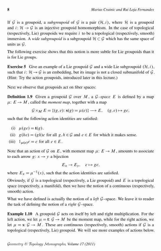
If G is a groupoid, a subgroupoid of G is a pair .H; i/, where H is a groupoidand i W H! G is an injective groupoid homomorphism. In the case of topological(respectively, Lie) groupoids we require i to be a topological (respectively, smooth)immersion. A wide subgroupoid is a subgroupoid H� G which has the same space ofunits as G .
The following exercise shows that this notion is more subtle for Lie groupoids than itis for Lie groups.
Exercise 5 Give an example of a Lie groupoid G and a wide Lie subgroupoid .H; i/,such that i W H! G is an embedding, but its image is not a closed submanifold of G .(Hint: Try the action groupoids, introduced later in this lecture.)
Next we observe that groupoids act on fiber spaces:
Definition 1.9 Given a groupoid G over M , a G–space E is defined by a map�W E!M , called the moment map, together with a map
G �M E D f.g; e/W s.g/D �.e/g �!E; .g; e/ 7! ge;
such that the following action identities are satisfied:
(i) �.ge/D t.g/.(ii) g.he/D .gh/e for all g; h 2 G and e 2E for which it makes sense.
(iii) 1�.e/e D e for all e 2E .
Note that an action of G on E , with moment map �W E!M , amounts to associateto each arrow gW x! y a bijection
Ex!Ey ; e 7! ge;
where Ex D ��1.x/, such that the action identities are satisfied.
Obviously, if G is a topological (respectively, a Lie groupoid) and E is a topologicalspace (respectively, a manifold), then we have the notion of a continuous (respectively,smooth) action.
What we have defined is actually the notion of a left G–space. We leave it to readerthe task of defining the notion of a right G–space.
Example 1.10 A groupoid G acts on itself by left and right multiplication. For theleft action, we let �D tW G!M be the moment map, while for the right action, welet � D sW G ! M . These are continuous (respectively, smooth) actions if G is atopological (respectively, Lie) groupoid. We will see more examples of actions below.
Geometry & Topology Monographs, Volume 17 (2011)

Lectures on integrability of Lie brackets 9
We mention here one more important notion, which is a simple extension of the notionof representations of groups, and which corresponds to linear groupoid actions.
Definition 1.11 Given a (topological, Lie) groupoid G over M , a representation of Gconsists of a vector bundle �W E!M , together with a (continuous, smooth) linearaction of G on E!M : for any arrow of G , gW x �! y , one has an induced linearisomorphism Ex!Ey , denoted v 7! gv , such that the action identities are satisfied.
Note that, in particular, each fiber Ex is a representation of the isotropy Lie group Gx .
There is an obvious notion of isomorphism of two representations and the isomorphismclasses of representations of a groupoid G form a semiring .Rep.G/;˚;˝/, where, fortwo representations E1 and E2 of G , the induced actions on E1˚E2 and E1˝E2
are the diagonal ones. The unit element is given by the trivial representation, ie, thetrivial line bundle LM over M with g � 1D 1.
1.3 First examples of Lie groupoids
Let us list some examples of groupoids. We start with two extreme classes of groupoidswhich, in some sense, are of opposite nature.
Example 1.12 (Groups) A group is the same thing as a groupoid for which theset of objects contains a single element. So groups are very particular instances ofgroupoids. Obviously, topological (respectively, Lie) groups are examples of topological(respectively, Lie) groupoids.
Example 1.13 (The pair groupoid) At the other extreme, let M be any set. TheCartesian product M �M is a groupoid over M if we think of a pair .y;x/ as anarrow x �! y . Composition is defined by
.z;y/.y;x/D .z;x/:
If M is a topological space (respectively, a manifold), then the pair groupoid is atopological (respectively, Lie) groupoid.
Note that each representation of the pair groupoid is isomorphic to a trivial vectorbundle with the tautological action. Hence
Rep.M �M /DN;
the semiring of nonnegative integers.
Geometry & Topology Monographs, Volume 17 (2011)

10 Marius Crainic and Rui Loja Fernandes
Our next examples are genuine examples of groupoids, which already exhibit somedistinct features.
Example 1.14 (General linear groupoids) If E is a vector bundle over M , thereis an associated general linear groupoid, denoted by GL.E/, which is similar to thegeneral linear group GL.V / associated to a vector space V . GL.E/ is a groupoidover M whose arrows between two points x and y consist of linear isomorphismsEx �!Ey , and the multiplication of arrows is given by the composition of maps.
Note that, given a general Lie groupoid G and a vector bundle E over M , a linear actionof G on E (making E into a representation) is the same thing as a homomorphism ofLie groupoids G! GL.E/.
Example 1.15 (The action groupoid) Let G �M !M be a smooth action of a Liegroup G on a manifold M . The corresponding action groupoid over M , denotedG ËM , has as space of arrows the Cartesian product
G DG �M:
For an arrow .g;x/ 2 G its source and target are given by
s.g;x/D x; t.g;x/D g �x;
while the composition of two arrows is given by
.h;y/.g;x/D .hg;x/:
Notice that the orbits and isotropy groups of G coincide with the usual notions of orbitsand isotropy groups of the action G �M !M . Also,
Rep.G ËM /D VectG.M /;
the semiring of equivariant vector bundles over M .
Example 1.16 (The gauge groupoid) If G is a Lie group and P �!M is a principalG –bundle, then the quotient of the pair groupoid P �P by the (diagonal) action of G
is a groupoid over P=G DM , denoted P ˝G P , and called the gauge groupoid of P .Note that all isotropy groups are isomorphic to G . Also, fixing a point x 2M , arepresentation E of P˝G P is uniquely determined by Ex 2Rep.G/, and this definesan isomorphism of semirings:
Rep.P ˝G P /� Rep.G/:
A particular case is when G D GLn and P is the frame bundle of a vector bundle E
over M of rank n. Then the resulting gauge groupoid coincides with GL.E/ mentionedabove.
Geometry & Topology Monographs, Volume 17 (2011)

Lectures on integrability of Lie brackets 11
Example 1.17 (The fundamental groupoid of a manifold) Closely related to the pairgroupoid of a manifold M is the fundamental groupoid of M , denoted …1.M /, whichconsists of homotopy classes of paths with fixed end points (we assume that M isconnected). In the light of Example 1.16, this is the gauge groupoid associated to theuniversal cover of M , viewed as a principal bundle over M with structural groupthe fundamental group of M , and this point of view also provides us with a smoothstructure on …1.M /, making it into a Lie groupoid. Note also that, when M is simplyconnected, …1.M / is isomorphic to the pair groupoid M �M (a homotopy class ofa path is determined by its end points). In general, there is an obvious homomorphismof Lie groupoids …1.M / �!M �M , which is a local diffeomorphism.
Exercise 6 Show that representations of …1.M / correspond to vector bundles over M
endowed with a flat connection.
Example 1.18 (The fundamental groupoid of a foliation) More generally, let F be afoliation of a space M of class C r (0 � r �1). The fundamental groupoid of F ,denoted by …1.F/, consists of the leafwise homotopy classes of paths (relative to theend points):
…1.F/D fŒ � W W Œ0; 1�!M a path lying in a leafg :
For an arrow Œ � 2…1.F/ its source and target are given by
s.Œ �/D .0/; t.Œ �/D .1/;
while the composition of two arrows is just concatenation of paths:
Œ 1�Œ 2�D Œ 1 � 2�;
the homotopy class of the concatenation of 2 with 1 .
In this example, the orbit Ox coincides with the leaf L through x , while the isotropygroup …1.F/x coincides with the fundamental group �1.L;x/.
Exercise 7 Verify that if F is a foliation of class C r (0� r �1) then …1.F/ is agroupoid of class C r .
The next exercise gives a simple example of a non-Hausdorff Lie groupoid.
Exercise 8 Let F be the smooth foliation of R3�f0g by horizontal planes. Checkthat the Lie groupoid …1.F/ is not Hausdorff.
Geometry & Topology Monographs, Volume 17 (2011)

12 Marius Crainic and Rui Loja Fernandes
1.4 The Lie algebroid of a Lie groupoid
Motivated by what we know about Lie groups, it is natural to wonder what are theinfinitesimal objects that correspond to Lie groupoids, and these ought to be called Liealgebroids.
Let us recall how we construct a Lie algebra out of a Lie group: if G is a Lie group,then its Lie algebra Lie.G/ consists of:
� An underlying vector space, which is just the tangent space to G at the unitelement.
� A Lie bracket on Lie.G/, which comes from the identification of Lie.G/ withthe space Xinv.G/ of right invariant vector fields on G , together with the factthat the space of right invariant vector fields is closed under the usual Lie bracketof vector fields:
ŒXinv.G/;Xinv.G/�� Xinv.G/:
Now, back to general Lie groupoids. One remarks two novelties when comparing withthe Lie group case. First of all, there is more than one unit element. In fact, there isone unit for each point in M , hence we expect a vector bundle over M , instead of avector space. Secondly, the right multiplication by elements of G is only defined onthe s–fibers. Hence, to talk about right invariant vector fields on G , we have to restrictattention to those vector fields which are tangent to the s–fibers, ie, to the sections ofthe subbundle T sG of T G defined by
T sG D Ker.ds/� T G:
Having in mind the discussion above, we first define Lie.G/ as a vector bundle over M .
Definition 1.19 Given a Lie groupoid G over M , we define the vector bundle AD
Lie.G/ whose fiber at x 2M coincides with the tangent space at the unit 1x of thes–fiber at x . In other words
A WD T sGjM :
Next, we describe the Lie bracket of the Lie algebroid A. This is, in fact, a bracketon the space of sections �.A/, and to deduce it we will identify the space �.A/ withthe space of right invariant vector fields on G . To see this, we observe that the fiber ofT s.G/ at an arrow hW y �! z is
T shG D ThG.y;�/;
Geometry & Topology Monographs, Volume 17 (2011)

Lectures on integrability of Lie brackets 13
so, for any arrow gW x �! y , the differential of the right multiplication by g inducesa map
RgW TshG! T s
hgG:Hence, we can describe the space of right invariant vector fields on G as
Xsinv.G/D
˚X 2 �.T sG/ WXhg DRg.Xh/; 8 .h;g/ 2 G2
:
Now, given ˛ 2 �.A/, the formula
zg DRg.˛t.g//
clearly defines a right invariant vector field. Conversely, any vector field X 2 Xsinv.G/
arises in this way: the invariance of X shows that X is determined by its values at thepoints in M :
Xg DRg.Xy/ for all gW x �! y;
ie, X D z where ˛ WD X jM 2 �.A/. Hence, we have shown that there exists anisomorphism
.1:20/ �.A/��! Xs
inv.G/; ˛ 7! z:
On the other hand, the space Xsinv.G/ is a Lie subalgebra of the Lie algebra X.G/ of
vector fields on G with respect to the usual Lie bracket of vector fields. This is clearsince the pullback of vector fields on the s–fibers, along Rg , preserves brackets.
Definition 1.21 The Lie bracket on A is the Lie bracket on �.A/ obtained from theLie bracket on Xinv.G/ under the isomorphism (1.20).
Hence the bracket on �.A/, which we denote by Œ � ; � �A (or simply Œ � ; � �, when thereis no danger of confusion) is uniquely determined by the formula
.1:22/ AŒ˛; ˇ�A D Œz; z�:To describe the entire structure of A, we need one more piece.
Definition 1.23 The anchor map of A is the bundle map
�AW A! TM
obtained by restricting dtW T G! TM to A� T G .
Again, when there is no danger of confusion (eg, in the discussion below), we simplywrite � instead of �A . The next proposition shows that the bracket and the anchor arerelated by a Leibniz-type identity. We use the notation LX for the Lie derivative alonga vector field.
Geometry & Topology Monographs, Volume 17 (2011)

14 Marius Crainic and Rui Loja Fernandes
Proposition 1.24 For all ˛; ˇ 2 �.A/ and all f 2 C1.M /,
Œ˛; fˇ�D f Œ˛; ˇ�CL�.˛/.f /ˇ:
Proof We use the characterization of the bracket (1.22). First note that efˇ D .f ıt/ z.From the usual Leibniz identity of vector fields (on G ),
BŒ˛; fˇ�D Œz;ffˇ�D Œz; .f ı t/ z�
D .f ı t/Œz; z�CLz.f ı t/ z:
But, at a point gW x �! y in G , we find
Lz.f ı t/.g/D dg.f ı t/.z.g//D dt.g/f ı d1t.g/ t.˛.t.g///D dt.g/f ı dgt.z.g//D L�.˛/.f /.t.g//:
Hence, we conclude that
BŒ˛; fˇ� DBf Œ˛; ˇ�C DL�.˛/.f /ˇ;and the result follows.
We summarize this discussion in the following definition:
Definition 1.25 The Lie algebroid of the Lie groupoid G is the vector bundle A D
Lie.G/, together with the anchor �AW A! TM and the Lie bracket Œ � ; � �A on �.A/.
Exercise 9 For each example of a Lie groupoid furnished in the paragraph above,determine its Lie algebroid.
To complete our analogy with the Lie algebra of a Lie group, and introduce theexponential map of a Lie groupoid, we set:
Definition 1.26 For x 2M , we put
�t˛.x/ WD �
tz.1x/ 2 G
where �tz
is the flow of the right invariant vector field z induced by ˛ . We call �t˛
the flow of ˛ .
Geometry & Topology Monographs, Volume 17 (2011)

Lectures on integrability of Lie brackets 15
Remark 1.27 The relevance of the flow comes from the fact that it provides the bridgebetween sections of A (infinitesimal data) and elements of G (global data). In fact,building on the analogy with the exponential map of a Lie group and Remark 1.7,we see that the flow of sections can be interpreted as defining an exponential mapexpW �.A/! �.G/ to the group of bisections of G :
exp.˛/.x/D �1˛.x/:
This is defined provided ˛ behaves well enough (eg, if it has compact support). Thisshows that, in some sense, �.A/ is the Lie algebra of �.G/.
Using the exponential notation, we can write the flow as �t˛ D exp.t˛/. The next
exercise will show that, just as for Lie groups, exp.t˛/ contains all the informationneeded to recover the entire flow of z .
Exercise 10 For ˛ 2 �.A/, show that:
(a) For all y 2M , �t˛.y/W y �! �t
�.˛/.y/.(b) For all gW x �! y in G , �t
z.g/ W x �! �t
�.˛/.y/, and �tz.g/D �t
˛.y/g .
(Here, �t�.˛/ is the flow of the vector field �.˛/ on M ).
1.5 Particular classes of groupoids
There are several particular classes of groupoids that deserve special attention, due totheir relevance both in the theory and in various applications.
First of all, recall that a topological space X is called k –connected (where k � 0 isan integer) if �i.X / is trivial for all 0� i � k and all base points.
Definition 1.28 A topological groupoid G over a space M is called source k –connected if the s–fibers s�1.x/ are k –connected for every x 2M . When k D 0 wesay that G is a s–connected groupoid, and when k D 1 we say that G is a s–simplyconnected groupoid.
Remark 1.29 One can show that a source n–connected Lie groupoid G over a n–connected base M has a space of arrows which is n–connected (see, eg, [26]).
Most of the groupoids that we will meet in these lectures are source-connected. Any Liegroupoid G has an associated source-connected groupoid G0 – the source-connectedcomponent of the identities. More precisely, G0�G consists of those arrows gW x�!y
of G which are in the connected component of G.x;�/ containing 1x .
Proposition 1.30 For any Lie groupoid, G0 is an open subgroupoid of G . Hence, G0
is a s–connected Lie groupoid that has the same Lie algebroid as G .
Geometry & Topology Monographs, Volume 17 (2011)

16 Marius Crainic and Rui Loja Fernandes
Proof Note that right multiplication by an arrow gW x �! y is a homeomorphismfrom s�1.y/ to s�1.x/. Therefore, it maps connected components to connectedcomponents. If g belongs to the connected component of s�1.x/ containing 1x , thenright multiplication by g maps 1y to g , so it maps the connected component of 1y tothe connected component of 1x . Hence G0 is closed under multiplication. Moreover,g�1 is mapped to 1x , so that g�1 belongs to the connected component of 1y , andhence G0 is closed under inversion. This shows that G0 is a subgroupoid.
To check that G0 is open, it is enough to observe that there exists an open neigh-borhood U of the identity section M � G which is contained in G0 . To see that,observe that by the local normal form of submersions, each 1x 2 G has an openneighborhood Ux which intersects each s–fiber in a connected set, ie, Ux � G0 . ThenU D
Sx2M Ux is the desired neighborhood.
Exercise 11 Is this proposition still true for topological groupoids?
Analogous to simply connected Lie groups and their role in standard Lie theory,groupoids which are s–simply connected play a fundamental role in the Lie theory ofLie groupoids.
Theorem 1.31 Let G be a s–connected Lie groupoid. There exist a Lie groupoid zGand homomorphism F W zG! G such that:
(i) zG is s–simply connected.
(ii) zG and G have the same Lie algebroid.
(iii) F is a local diffeomorphism.
Moreover, zG is unique up to isomorphism.
Proof We define the new groupoid zG by letting zG.x;�/ be the universal cover ofG.x;�/ consisting of homotopy classes (with fixed end points) of paths starting at 1x .Given gW I ! G representing a homotopy class Œg� 2 zG , we set s.Œg�/ WD s.g.0//and t.Œg�/ WD t.g.1//. Given Œg1�; Œg2� 2 zG composable, we define Œg1� � Œg2� as thehomotopy class of the concatenation of g2 with Rg2.1/ ıg1 . (Draw a picture!)
It is easy to check that zG is a groupoid. To describe its smooth structure, one remarksthat zG D p�1.M /, where pW …1.F.s//! G is the source map of the fundamentalgroupoid of the foliation on G by the fibers of s. Since p is a submersion, zG will besmooth and of the same dimension as G . It is not difficult to check that the structuremaps are also smooth. The projection F W zG! G which sends Œg� to g.1/ is clearly a
Geometry & Topology Monographs, Volume 17 (2011)

Lectures on integrability of Lie brackets 17
surjective groupoid morphism (G is s–connected), which is easily seen to be a localdiffeomorphism. Hence, it induces an isomorphism at the level of algebroids. We leavethe proof of uniqueness as an exercise.
At the opposite extreme of s–connectedness there are the groupoids that model the leafspaces of foliations, known as étale groupoids.
Definition 1.32 A Lie groupoid G is called étale if its source map s is a local diffeo-morphism.
Example 1.33 Here are a few simple examples of étale groupoids:
(1) Any manifold M can be viewed as an étale groupoid with identity elementsonly.
(2) The fundamental groupoid of a foliation is not étale in general. However, let T
be a complete transversal, ie, an immersed submanifold which intersects everyleaf, and is transversal at each intersection point (note that T does not have to beconnected). Then, each holonomy transformation determines an arrow betweenpoints of T , and so they form a groupoid Hol.T /� T , which is étale.2
(3) An action groupoid G D G ËM is étale if and only if G is discrete. To seethis, just notice that sW G!M is the projection s.g;m/Dm, so it is a localdiffeomorphism if and only if G is discrete.
Exercise 12 Show that a Lie groupoid is étale if and only if its source fibers arediscrete.
Analogous to compact Lie groups are proper Lie groupoids, which define anotherimportant class.
Definition 1.34 A Lie groupoid G over M is called proper if the map .s; t/W G !M �M is a proper map.
We will see that, for proper groupoids, any representation admits an invariant metric.The following exercise asks you to prove some other basic properties of proper Liegroupoids.
Exercise 13 Let G be a proper Lie groupoid over M . Show that:
(a) All isotropy groups of G are compact.(b) All orbits of G are closed submanifolds.(c) The orbit space M=G is Hausdorff.
2 The resulting groupoid is equivalent to the fundamental groupoid of the foliation, in a certain sensethat can be made precise.
Geometry & Topology Monographs, Volume 17 (2011)
18 Marius Crainic and Rui Loja Fernandes
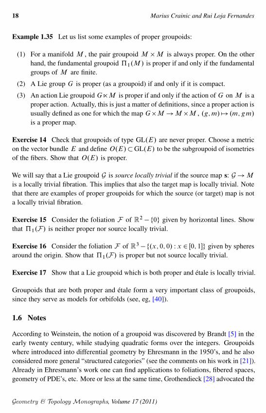
Example 1.35 Let us list some examples of proper groupoids:
(1) For a manifold M , the pair groupoid M �M is always proper. On the otherhand, the fundamental groupoid …1.M / is proper if and only if the fundamentalgroups of M are finite.
(2) A Lie group G is proper (as a groupoid) if and only if it is compact.
(3) An action Lie groupoid GËM is proper if and only if the action of G on M is aproper action. Actually, this is just a matter of definitions, since a proper action isusually defined as one for which the map G�M !M �M , .g;m/ 7! .m;gm/
is a proper map.
Exercise 14 Check that groupoids of type GL.E/ are never proper. Choose a metricon the vector bundle E and define O.E/�GL.E/ to be the subgroupoid of isometriesof the fibers. Show that O.E/ is proper.
We will say that a Lie groupoid G is source locally trivial if the source map sW G!M
is a locally trivial fibration. This implies that also the target map is locally trivial. Notethat there are examples of proper groupoids for which the source (or target) map is nota locally trivial fibration.
Exercise 15 Consider the foliation F of R2 � f0g given by horizontal lines. Showthat …1.F/ is neither proper nor source locally trivial.
Exercise 16 Consider the foliation F of R3�f.x; 0; 0/ W x 2 Œ0; 1�g given by spheresaround the origin. Show that …1.F/ is proper but not source locally trivial.
Exercise 17 Show that a Lie groupoid which is both proper and étale is locally trivial.
Groupoids that are both proper and étale form a very important class of groupoids,since they serve as models for orbifolds (see, eg, [40]).
1.6 Notes
According to Weinstein, the notion of a groupoid was discovered by Brandt [5] in theearly twenty century, while studying quadratic forms over the integers. Groupoidswhere introduced into differential geometry by Ehresmann in the 1950’s, and he alsoconsidered more general “structured categories” (see the comments on his work in [21]).Already in Ehresmann’s work one can find applications to foliations, fibered spaces,geometry of PDE’s, etc. More or less at the same time, Grothendieck [28] advocated the
Geometry & Topology Monographs, Volume 17 (2011)

Lectures on integrability of Lie brackets 19
use of groupoids in algebraic geometry as the right notion to understand moduli spaces(in the spirit of the introductory section in this lecture), and from that the theory ofstacks emerged; see Behrend et al [3]. Important sources of examples, which stronglyinfluenced the theory of Lie groupoids, comes from Haefliger’s approach to transversalgeometry of foliations, from Connes’ noncommutative geometry [11] and from Poissongeometry (see the announcement of Weinstein [56] and the first systematic expositionof symplectic groupoids by Coste, Dazord and Weinstein [12]), with independentcontributions from others, notably Karasëv [34] and Zakrzewski [65]).
The book of MacKenzie [36] contains a nice introduction to the theory of transitive andlocally trivial groupoids, which has now been superseded by his new book [38], wherehe also treats nontransitive groupoids and double structures. The modern approach togroupoids can also be found in recent monographs, such as the book by Cannas da Silvaand Weinstein [51] devoted to the geometry of noncommutative objects, the book byMoerdijk and Mrcun [43] on Lie groupoids and foliations, and the book by Dufour andZung [19] on Poisson geometry.
Several important aspects of Lie groupoid theory have not made it yet to expositorybooks. Let us mentioned as examples the theory of proper Lie groupoids (see, eg, thepapers by Crainic [14], Weinstein [59] and Zung [66]), the theory of differentiablestacks, gerbes and nonabelian cohomology (see, eg, the preprints by Behrend andXu [4] and Moerdijk [41]).
As time progresses, there are also a few aspects of Lie groupoid theory that seem to havelost interest or simply disappeared. We feel that some of these are worth recovering andwe mention two examples. A prime example is provided by Haefliger’s approach tointegrability and homotopy theory (see the beautiful article of Haefliger [30]). Anotherremarkable example is the geometric approach to the theory of PDE’s sketched byEhresmann’s, with roots in É Cartan’s pioneer works, and which essentially came to anhalt with the monograph by Kumpera and Spencer [35].
2 Lie algebroids
2.1 Why algebroids?
We saw in Lecture 1 that Lie groupoids are natural objects to study in differentialgeometry. Moreover, to every Lie groupoid G over M there is associated a certainvector bundle A!M , which carries additional structure, namely a Lie bracket on thesections and a bundle map A! TM . If one axiomatizes these properties, one obtainsthe abstract notion of a Lie algebroid:
Geometry & Topology Monographs, Volume 17 (2011)

20 Marius Crainic and Rui Loja Fernandes
Definition 2.1 A Lie algebroid over a manifold M consists of a vector bundle A
together with a bundle map �AW A! TM and a Lie bracket Œ ; �A on the space ofsections �.A/, satisfying the Leibniz identity
Œ˛; fˇ�A D f Œ˛; ˇ�ACL�A.˛/.f /ˇ;
for all ˛; ˇ 2 �.A/ and all f 2 C1.M /.
Exercise 18 Prove that the induced map �AW �.A/! X.M / is a Lie algebra homo-morphism.
Before we dive into the study of Lie algebroids, we would like to show that Liealgebroids are interesting by themselves, independently of Lie groupoids. In fact, ingeometry one is led naturally to study Lie algebroids and, in their study, it is useful tointegrate them to Lie groupoids!
In order to illustrate this point, just like we did at the beginning of Lecture 1, we lookagain at equivalence problems in geometry. Élie Cartan observed that many equivalenceproblems in geometry can be best formulated in terms of coframes. Working out thecoframe formulation, he was able to come up with a method, now called Cartan’sequivalence method, to deal with such problems.
A local version of Cartan’s formulation of equivalence problems can be described asfollows: one is given a family of functions ci
j ;k, ba
i defined on some open set U �Rn ,where the indices satisfy 1� i; j ; k � r , 1� a� n (n, r positive integers). Then theproblem is:
Cartan’s Problem Find a manifold N , a coframe f�ig on N and a function hW N!U ,satisfying the equations
d�iD
Xj ;k
cij ;k.h/�
j^ �k ;.2:2/
dhaD
Xi
bai .h/�
i :.2:3/
As part of this problem we should be able to answer the following questions:
� When does Cartan’s problem have a solution?
� What are the possible solutions to Cartan’s problem?
Here is a simple, but interesting, illustrative example:
Geometry & Topology Monographs, Volume 17 (2011)

Lectures on integrability of Lie brackets 21
Example 2.4 Let us consider the problem of equivalence of metrics in R2 withconstant Gaussian curvature. If ds2 is a metric in R2 then there exists a diagonalizingcoframe f�1; �2g, so that
ds2D .�1/2C .�2/2:
In terms of Cartesian coordinates, this coframe can be written as
�1DA dxCB dy; �2
D C dxCD dy;
where A;B;C;D are smooth functions of .x;y/ satisfying AD�BC 6D 0. Takingexterior derivatives, we obtain
d�1D J�1
^ �2; d�2DK�1
^ �2;.2:5/
J DBx �Ay
AD�BC; K D
Dx �Cy
AD�BC:where
If f is any smooth function in R2 , the coframe derivatives of f relative to f�1; �2g
are defined to be the coefficients of the differential df when expressed in terms of thecoframe:
df D@f
@�1�1C@f
@�2�2:
For example, the Gaussian curvature of ds2 is given in terms of the coframe derivativesof the structure functions by
� D@J
@�2�@K
@�1�J 2
�K2:
So we see that for metrics of constant Gaussian curvature, the two structure functionsJ and K are not independent, and we can choose one of them as the independent one,say J . Then we can write
.2:6/ dJ DL�1^ �2:
Equations (2.5) and (2.6) form the structure equations of the Cartan problem of clas-sifying metrics of constant Gaussian curvature. Using these equations one can findnormal forms for all metrics of constant Gaussian curvature.
Exercise 19 Show that the metrics of zero Gaussian curvature (� D 0) can be reducedto the following form:
ds2D dx2
C dy2:
Obvious necessary conditions to solve Cartan’s problem can be obtained as immediateconsequences of the fact that d2 D 0 and that f�ig is a coframe. In fact, a simple
Geometry & Topology Monographs, Volume 17 (2011)
22 Marius Crainic and Rui Loja Fernandes
computation gives3
Fbi .h/
@Faj
@hb.h/�Fb
j .h/@Fa
i
@hb.h/D�cl
i;j .h/Fal .h/;.2:7/
Faj .h/
@cik;l
@ha.h/CFa
k .h/@ci
l;j
@ha.h/CFa
l .h/@ci
j ;k
@ha.h/
D��ci
m;j .h/cmk;l.h/C ci
mk.h/cml;j .h/C ci
m;l.h/cmj ;k.h/
�:
.2:8/
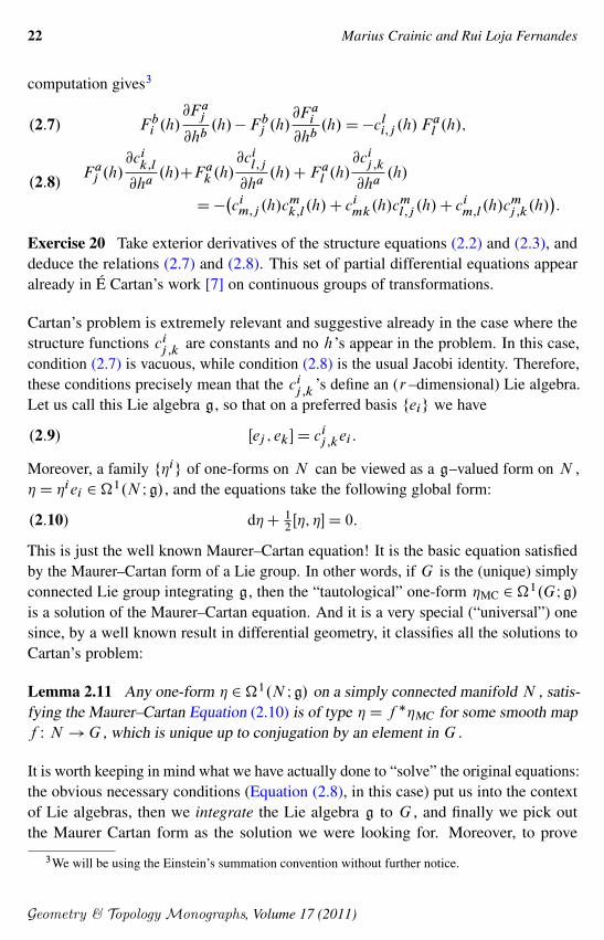
Exercise 20 Take exterior derivatives of the structure equations (2.2) and (2.3), anddeduce the relations (2.7) and (2.8). This set of partial differential equations appearalready in É Cartan’s work [7] on continuous groups of transformations.
Cartan’s problem is extremely relevant and suggestive already in the case where thestructure functions ci
j ;kare constants and no h’s appear in the problem. In this case,
condition (2.7) is vacuous, while condition (2.8) is the usual Jacobi identity. Therefore,these conditions precisely mean that the ci
j ;k’s define an (r –dimensional) Lie algebra.
Let us call this Lie algebra g, so that on a preferred basis feig we have
.2:9/ Œej ; ek �D cij ;kei :
Moreover, a family f�ig of one-forms on N can be viewed as a g–valued form on N ,�D �iei 2�
1.N I g/, and the equations take the following global form:
.2:10/ d�C 12Œ�; ��D 0:
This is just the well known Maurer–Cartan equation! It is the basic equation satisfiedby the Maurer–Cartan form of a Lie group. In other words, if G is the (unique) simplyconnected Lie group integrating g, then the “tautological” one-form �MC 2�
1.GI g/
is a solution of the Maurer–Cartan equation. And it is a very special (“universal”) onesince, by a well known result in differential geometry, it classifies all the solutions toCartan’s problem:
Lemma 2.11 Any one-form � 2�1.N I g/ on a simply connected manifold N , satis-fying the Maurer–Cartan Equation (2.10) is of type �D f ��MC for some smooth mapf W N !G , which is unique up to conjugation by an element in G .
It is worth keeping in mind what we have actually done to “solve” the original equations:the obvious necessary conditions (Equation (2.8), in this case) put us into the contextof Lie algebras, then we integrate the Lie algebra g to G , and finally we pick outthe Maurer Cartan form as the solution we were looking for. Moreover, to prove
3We will be using the Einstein’s summation convention without further notice.
Geometry & Topology Monographs, Volume 17 (2011)

Lectures on integrability of Lie brackets 23
its universality (see the Lemma), we had to produce a map f W N ! G out of aform � 2 �1.N I g/. Viewing � as a map �W TN ! g, we may say that we have“integrated �”.
Now what if we allow the h into the picture, and try to extend this piece of basicgeometry to the general equations? This leads us immediately to the world of algebroids!Since the structure functions ci
j ;kare no longer constant (they depend on h 2 U ), the
brackets they define (2.9) make sense provided feig depend themselves on h. Ofcourse, feig can then be viewed as trivializing sections of an r –dimensional vectorbundle A over U . On the other hand, the functions ba
i are the components of a map
�.A/ 3 ei 7�! bai
@
@xa2 X.U /:
The necessary conditions (2.7) and (2.8) are just the conditions that appear in thedefinition of a Lie algebroid. This is the content of the next exercise.
Exercise 21 Let A be a Lie algebroid over a manifold M . Pick an open coordinateneighborhood U �M , with coordinates .xa/ and a basis of sections feig that trivializethe bundle AjU . Also, define structure functions ci
j ;kand ba
i by
Œej ; ek �D cij ;kei ; �.ei/D ba
i
@
@xa:
Check that Equation (2.7) is equivalent to the condition that � is a Lie algebra homo-morphism:
Œ�.ej /; �.ek/�D �.Œej ; ek �/;
and that Equation (2.8) is equivalent to the Jacobi identity:
Œei ; Œej ; ek ��C Œej ; Œek ; ei ��C Œek ; Œei ; ej ��D 0:
What about the associated global objects and the associated Maurer Cartan forms? Ourobjective here is not to give a detailed discussion of Cartan’s problem, but it is nothard to guess that, in the end, you will find Lie algebroid valued forms and that youwill need to integrate the Lie algebroid, eventually rediscovering the notion of a Liegroupoid.
After this motivating example, it is now time to start our study of Lie algebroids.
2.2 Lie algebroids
Let A be a Lie algebroid over M . We start by looking at the kernel and at the imageof the anchor �W A! TM .
Geometry & Topology Monographs, Volume 17 (2011)

24 Marius Crainic and Rui Loja Fernandes
If we fix x 2 M , the kernel Ker.�x/ is naturally a Lie algebra: if ˛; ˇ 2 �.A/lie in Ker.�x/ when evaluated at x , the Leibniz identity implies that Œ˛; fˇ�.x/ Df .x/Œ˛; ˇ�.x/. Hence, there is a well defined bracket on Ker.�x/ such that
Œ˛.x/; ˇ.x/�Ker.�x/ D Œ˛; ˇ�A.x/:
for ˛ and ˇ as above.
Definition 2.12 At any point x 2M the Lie algebra
gx.A/ WD Ker.�x/;
is called the isotropy Lie algebra at x .
Exercise 22 Let G be a s–connected Lie groupoid over M and let A be its Liealgebroid. Show that the isotropy Lie algebra gx.A/ is isomorphic to the Lie algebraof the isotropy Lie group Gx , for all x 2M .
Let us now look at the image of the anchor. This gives a distribution
M 3 x 7! Im.�x/� TxM;
of subspaces whose dimension, in general, will vary from point to point. If the rankof � is constant we say that A is a regular Lie algebroid.
Exercise 23 If A is a regular Lie algebroid show that the resulting distribution is inte-grable, so that M is foliated by immersed submanifolds O ’s, called orbits, satisfyingTxOD Im.�x/ forall x 2O .
For a general Lie algebroid A there is still an induced partition of M by immersedsubmanifolds, called the orbits of A. As in the regular case, one looks for maximalimmersed submanifolds O ’s satisfying
TxOD Im.�x/;
for all x 2 O . Their existence is a bit more delicate in the nonregular case. Onepossibility is to use a Frobenius type theorem for singular foliations. However, there isa simple way of describing the orbits, at least set theoretically. This uses the notionof A–path, which will play a central role in the integrability problem to be studied inLecture 3.
Geometry & Topology Monographs, Volume 17 (2011)

Lectures on integrability of Lie brackets 25
Definition 2.13 Given a Lie algebroid A over M , an A–path consists of a pair .a; /where W I !M is a path in M , aW I !A is a path in A4, such that:
(i) a is a path above , ie, a.t/ 2A .t/ for all t 2 I .
(ii) �.a.t//D d dt.t/ for all t 2 I .
Of course, a determines the base path , hence when talking about an A–path we willonly refer to a. The reason we mention in the previous definition is to emphasizethe way we think of A–paths: a should be interpreted as an “A–derivative of ”, andthe last condition in the definition should be read: “the usual derivative of is relatedto the A–derivative by the anchor map”.
We can now define an equivalence relation on M , denoted �A , as follows. We saythat x;y 2M are equivalent if there exists an A–path a, with base path , such that .0/D x and .1/D y . An equivalence class of this relation will be called an orbitof A. When � is surjective we say that A is a transitive Lie algebroid. In this case,each connected component of M is an orbit of A.
Remark 2.14 It remains to show that each orbit O is an immersed submanifold of M ,which integrates Im.�/, ie, TxOD Im.�x/ for all x 2O . This can be proved using alocal normal form theorem for Lie algebroids (see, eg, [17, Theorem 8.5.1]).
Exercise 24 Let G be a s–connected Lie groupoid over M and let A be its Liealgebroid. Show that the orbits of G in M coincide with the orbits of A in M . (Hint:Check that if g.t/W I ! G is a path that stays in a s–fiber and starts at 1x , thena.t/D dg.t/Rg.t/�1 � Pg.t/ is an A–path.)
As we saw in Lecture 1, any Lie groupoid has an associated Lie algebroid. For futurereference, we introduce the following terminology:
Definition 2.15 A Lie algebroid A is called integrable if it is isomorphic to the Liealgebroid of a Lie groupoid G . For such a G , we say that G integrates A.
Similar to Lie’s first theorem for Lie algebras (which asserts that there is at most onesimply connected Lie group integrating a given Lie algebra), we have the followingtheorem:
Theorem 2.16 (Lie I) If A is integrable, then there exists an unique (up to isomor-phism) s–simply connected Lie groupoid G integrating A.
4Here and below, I D Œ0; 1� will always denote the unit interval.
Geometry & Topology Monographs, Volume 17 (2011)

26 Marius Crainic and Rui Loja Fernandes
Proof This follows at once from Lecture 1, where we have shown that for any Liegroupoid G there exists a unique (up to isomorphism) Lie groupoid zG which is s–simply connected and which has the same Lie algebroid as G (see Theorem 1.31).
Let us turn now to morphisms of Lie algebroids.
Definition 2.17 Let A1!M1 and A2!M2 be Lie algebroids. A morphism of Liealgebroids is a vector bundle map
A1F //
��
A2
��M1
f
// M2
which is compatible with the anchors and the brackets.
Let us explain what we mean by compatible. First, we say that the map F W A1!A2
is compatible with the anchors if
df .�A1.a//D �A2
.F.a//:
This can be expressed by the commutativity of the diagram:
A1F //
�1
��
A2
�2
��TM1
df// TM2
Secondly, we would like to say what we mean by compatibility with the brackets. Thedifficulty here is that, in general, sections of A1 cannot be pushed forward to sectionsof A2 . Instead we have to work at the level of the pullback bundle f �A2 .5 Firstnote that from sections ˛ of A1 or ˛0 of A2 , we can produce new sections F.˛/ andf �.˛0/ of f �A2 by
F.˛/D F ı˛; f �.˛0/D ˛0 ıf:
Now, given any section ˛ 2�.A1/, we can express its image under F as a (nonunique)finite combination
F.˛/DX
i
cif�.˛i/;
5Alternative, more intrinsic, definitions will be described in Exercise 47 and Exercise 50.
Geometry & Topology Monographs, Volume 17 (2011)

Lectures on integrability of Lie brackets 27
where ci 2C1.M1/ and ˛i 2�.A2/. By compatibility with the brackets we mean that,if ˛; ˇ 2�.A1/ are sections such that their images are expressed as finite combinationsas above, then their bracket is a section whose image can be expressed as
.2:18/ F.Œ˛; ˇ�A1/D
Xi;j
cic0jf�Œ˛i ; j �A2
C
Xj
L�.˛/.c0j /f�. j /�
Xi
L�.ˇ/.ci/f�.˛i/:
Notice that, in the case where the sections ˛; ˇ 2 �.A1/ can be pushed forward tosections ˛0; ˇ0 2 �.A2/, so that F.˛/D ˛0 ı f and F.ˇ/D ˇ0 ı f , this just meansthat
F.Œ˛; ˇ�A1/D Œ˛0; ˇ0�A2
ıf:
The following exercises should help make you familiar with the notion of a Lie algebroidmorphism.
Exercise 25 Check that condition (2.18) is independent of the way one expresses theimage of the sections under F as finite combinations.
Exercise 26 Let A be a Lie algebroid. Show that a path aW Œ0; 1�!A is an A–pathif and only if the map a dt W TI !A is a morphism of Lie algebroids.
Exercise 27 Show that if F W G!H is a homomorphism of Lie groupoids, then itinduces a Lie algebroid homomorphism F W A! B of their Lie algebroids.
Again, just like in the case of Lie algebras, under a suitable assumption, we can integratemorphisms of Lie algebroids to morphisms of Lie groupoids:
Theorem 2.19 (Lie II) Let F W A! B be a morphism of integrable Lie algebroids,and let G and H be integrations of A and B . If G is s–simply connected, then thereexists a (unique) morphism of Lie groupoids F W G!H integrating F .
You may try to reproduce the proof that you know for the Lie algebra case. You willalso find a proof in Lecture 3 (see Exercise 64). The next exercise shows how to definethe exponential map for Lie algebroids/groupoids.
Exercise 28 Let A be the Lie algebroid of a Lie groupoid G . Use Lie II (Theorem 2.19)to define the exponential map expW �c.A/! �.G/, taking sections of compact supportto bisections of G . How does this relate to the construction hinted at in Remark 1.27?
Geometry & Topology Monographs, Volume 17 (2011)

28 Marius Crainic and Rui Loja Fernandes
2.3 First examples of Lie algebroids
Let us present now a few basic examples of Lie algebroids.
Example 2.20 (Tangent bundles) The most basic example of a Lie algebroid over M
is the tangent bundle A D TM , with the identity map as anchor, and the usual Liebracket of vector fields. Here the isotropy Lie algebras are trivial and the Lie algebroidis transitive.
Exercise 29 Prove that the Lie algebroids of the pair groupoid M �M and of thefundamental groupoid …1.M / are both isomorphic to TM .
Example 2.21 (Lie algebras) At the other extreme, Lie algebras g are the same thingas Lie algebroids over a one-point manifold; Lie groupoids integrating g are the sameas Lie groups whose Lie algebra is g.
Both these examples can be slightly generalized. For example, the tangent bundle canbe generalized as follows:
Example 2.22 (Foliations) Let A � TM be an involutive subbundle, ie, constantrank smooth distribution which is closed for the usual Lie bracket. This gives a Liealgebroid (in fact a Lie subalgebroid of TM ) over M , with anchor map the inclusion,and the Lie bracket the restriction of the usual Lie bracket of vector fields.
Recall that, by the Frobenius Integrability Theorem, A determines a foliation F of amanifold M (and conversely, every foliation determines a Lie algebroid TF � TM ).In fact, F is just the orbit foliation of A (see the discussion above). On the other hand,since the anchor is injective, the isotropy Lie algebras gx are all trivial.
Exercise 30 Prove that the Lie algebroid of the fundamental groupoid …1.F/ isisomorphic to TF . Can you give another example of a groupoid integrating TF ?
On the other hand, Lie algebras can be generalized as follows:
Example 2.23 (Bundles of Lie algebras) A bundle of Lie algebras over M is avector bundle A over M together with a Lie algebra bracket Œ � ; � �x on each fiber Ax ,which varies smoothly with respect to x in the sense that if ˛; ˇ 2 �.A/, then Œ˛; ˇ�defined by
Œ˛; ˇ�.x/D Œ˛.x/; ˇ.x/�x
Geometry & Topology Monographs, Volume 17 (2011)

Lectures on integrability of Lie brackets 29
is a smooth section of A. Note that this notion is weaker then that of Lie algebra bundle,when one requires that A is locally trivial as a bundle of Lie algebras (in particular, allthe Lie algebras Ax should be isomorphic).
Since the anchor is identically zero, the orbits of A are the points of M , while theisotropy Lie algebras are the fibers Ax . It is easy to see that a bundle of Lie algebrasover M is precisely the same thing as a Lie algebroid over M with zero anchor map.
A general Lie algebroid can be seen as combining aspects from both the previous twoexamples. In fact, take a Lie algebroid A over M and fix an orbit i W O ,!M . Inthe following exercise we ask you to check that the bracket restricts to a bracket onAO DAjO WD i�A.
Exercise 31 Let ˛; ˇ 2 �.AO/ be local sections, and z; z 2 �.A/ be any choice oflocal extensions. Show that
Œ˛; ˇ� WD Œz; z�jO;
is well-defined, ie, it is independent of the choice of extensions. (Hint: Since O is aleaf, the vector fields �.˛/ and �.ˇ/ are tangent to O .)
Since the restriction of the anchor gives a map �OW AO ! TO , we obtain a Liealgebroid structure on AO over O . On the other hand, one has an induced bundle ofLie algebras:
gO.A/D Ker.�O/;
whose fiber at x is the isotropy Lie algebra gx.A/. All these fit into a short exactsequence of algebroids over O
0 �! gO.A/ �!AO �! TO �! 0:
The isotropy bundle gO.A/ is actually a Lie algebra bundle, as indicated in the followingexercise.
Exercise 32 (a) Show that a bundle of Lie algebras gM !M is a Lie algebrabundle if and only if there exists a connection rW X.M /˝�.gM /! �.gM /
satisfyingrX .Œ˛; ˇ�/D ŒrX .˛/; ˇ�C Œ˛;rX .ˇ/�
for all ˛; ˇ 2 �.gM /.
(b) Deduce that each isotropy bundle gO.A/ is a Lie algebra bundle. In particular,all the isotropy Lie algebras gx.A/, with x 2O , are isomorphic.
(Hint: For (a), use parallel transport. For (b), use a splitting of �OW AjO! TO andthe bracket of AO to produce a connection.)
Geometry & Topology Monographs, Volume 17 (2011)
30 Marius Crainic and Rui Loja Fernandes
Example 2.24 (Vector fields) It is not difficult to see that Lie algebroid structureson the trivial line bundle over M are in 1–1 correspondence with vector fields on M .Given a vector field X , we denote by AX the induced Lie algebroid. Explicitly, as avector bundle, AX D LDM �R is the trivial line bundle, while the anchor is givenby multiplication by X , and the Lie bracket of two section f;g 2 �.AX /D C1.M /
is defined byŒf;g�D f LX .g/�LX .f /g:
Exercise 33 Find out how the flow of X defines an integration of AX .
Example 2.25 (Action Lie algebroid) Generalizing the Lie algebroid of a vectorfield, consider an infinitesimal action of a Lie algebra g on a manifold M , ie, a Liealgebra homomorphism �W g! X.M /. The standard situation is when g is the Liealgebra of a Lie group G that acts on M . Then
�.v/.x/ WDddt
exp.tv/x; v 2 g;x 2M;
defines an infinitesimal action of g on M . We say that an infinitesimal action of g
on M is integrable if it comes from a Lie group action.
Given an infinitesimal action of g on M , we form a Lie algebroid gËM , called theaction Lie algebroid, as follows. As a vector bundle, it is the trivial vector bundleM � g over M with fiber g, the anchor is given by the infinitesimal action, while theLie bracket is uniquely determined by the Leibniz identity and the condition that
Œcv; cw �D cŒv;w�;
for all v;w 2 g, where cv denotes the constant section of g.
Exercise 34 This exercise discusses the relationship between the integrability of Liealgebra actions and the corresponding action Lie algebroid:
(a) Given an action of a Lie group G on M , show that the corresponding action Liegroupoid G ËM over M has a Lie algebroid the action Lie algebroid gËM .Hence, if an infinitesimal action of g on M is integrable, then the Lie algebroidgËM is integrable.
(b) Find an infinitesimal action of a Lie algebra g which is not integrable but whichhas the property that the Lie algebroid g ËM is integrable. (Hint: Think ofvector fields!)
Exercise 35 Show that all action Lie algebroids gËM arising from infinitesimal Liealgebra actions are integrable. (Hint: Think again of what happens for vector fields!)
Geometry & Topology Monographs, Volume 17 (2011)

Lectures on integrability of Lie brackets 31
Example 2.26 (Two forms) Any closed 2–form ! on a manifold M has an associ-ated Lie algebroid, denoted A! , and defined as follows. As a vector bundle,
A! D TM ˚L;
the anchor is the projection on the first component, while the bracket on sections�.A!/' X.M /�C1.M / is defined by
Œ.X; f /; .Y;g/�D .ŒX;Y �;LX .g/�LY .f /C!.X;Y //:
Exercise 36 Given a 2–form on M , check that the previous formulas make A! intoa Lie algebroid if and only if ! is closed.
Example 2.27 (Atiyah sequences) Let G be a Lie group. To any principal G–bundle P over M there is an associated Lie algebroid over M , denoted A.P /, anddefined as follows. As a vector bundle, A.P / WD TP=G (over P=G D M ). Theanchor is induced by the differential of the projection from P to M . Also, since thesections of A.P / correspond to G –invariant vector fields on P , we see that there is acanonical Lie bracket on �.A.P //. With these, A.P / becomes a Lie algebroid.
Exercise 37 Show that A.P / is just the Lie algebroid of the gauge groupoid P˝G P .
Note that A.P / is transitive, ie, the anchor map is surjective. We denote by P Œg� thekernel of the anchor map. Hence we have a short exact sequence
0 �! P Œg� �!A.P / �! TM �! 0;
known as the Atiyah sequence associated to P . Of course, this is obtained by dividingout the action of G on the exact sequence of vector bundles over P : P�g�!TP �!
TM . In particular, P Œg� is the Lie algebra bundle obtained by attaching to P theadjoint representation of G .
One of the interesting things about the Atiyah sequence is its relation with connectionsand their curvatures. First of all, connections on the principal bundle P are the samething as splittings of the Atiyah sequence. Indeed, a left splitting of the sequence is thesame thing as a bundle map TP!P�g which is G –invariant, and which is left inverseto the infinitesimal action g! TP , in other words, a connection 1–form. By standardlinear algebra, left splittings of a short exact sequence are in 1–1 correspondence withright splittings. Henceforth, we will identify connections with left/right splittings.
Next, given a connection whose associated right splitting is denoted by � W TM!A.P /,the curvature of the connection is a 2–form on M with values in P Œg�, and can bedescribed using � and the Lie bracket on A.P /:
�� .X;Y /D Œ�.X /; �.Y /�� �.ŒX;Y �/:
Geometry & Topology Monographs, Volume 17 (2011)

32 Marius Crainic and Rui Loja Fernandes
Using these as motivations, transitive (ie, with surjective anchor) Lie algebroids A arealso called abstract Atiyah sequence, while splittings of their anchor map are calledconnections. The sequence associated to A is, of course,
0 �! Ker.�/ �!A �! TM �! 0:
Note that not all abstract Atiyah sequences come from principal bundles.
Exercise 38 Give an example of a transitive Lie algebroid which is not the Atiyahsequence of some principal bundle.
Example 2.28 (Poisson manifolds) Any Poisson structure on a manifold M inducesa Lie algebroid structure on T �M as follows. Let � be the Poisson bivector on M ,which is related to the Poisson bracket by ff;gg D �.df; dg/. Also, the Hamiltonianvector field Xf associated to a smooth function f on M is given by Xf .g/D ff;gg.We use the notation
�]W T �M ! TM
for the map defined by ˇ.�].˛// D �.˛; ˇ/. The Lie algebroid structure on T �M
has �] as anchor map, and the Lie bracket is defined by
Œ˛; ˇ�D L�].˛/.ˇ/�L�].ˇ/.˛/� d.�.˛; ˇ//:
We call this the cotangent Lie algebroid of the Poisson manifold .M; �/.
Exercise 39 Show that this Lie algebroid structure on T �M is the unique one with theproperty that the anchor maps df to Xf and Œdf; dg�D dff;gg forall f;g 2C1.M /.
Example 2.29 (Nijenhuis tensors) Given a bundle map N W TM ! TM , recall thatits Nijenhuis torsion, denoted TN 2 �.^
2T �M ˝TM /, is defined by
TN .X;Y /D ŒNX;NY ��N ŒNX;Y ��N ŒX;NY �CN 2ŒX;Y �;
for X;Y 2 X.M /. When TN D 0 we call N a Nijenhuis tensor. To any Nijenhuistensor N , there is associated a new Lie algebroid structure on TM : the anchor isgiven by �.X /DN .X /, while the Lie bracket is defined by
ŒX;Y �N WD ŒNX;Y �C ŒX;NY ��N .ŒX;Y �/:
This kind of Lie algebroid plays an important role in the theory of integrable systems,in the study of (generalized) complex structures, etc.
Geometry & Topology Monographs, Volume 17 (2011)

Lectures on integrability of Lie brackets 33
Exercise 40 Thinking of a Lie algebroid as a generalized tangent bundle, extend thisconstruction to any Lie algebroid A!M : given a bundle map N W A!A over theidentity, such that its Nijenhuis torsion vanishes, ie,
ŒN˛;Nˇ�A�N ŒN˛; ˇ�A�N Œ˛;Nˇ�ACN 2Œ˛; ˇ�A D 0;
for all ˛; ˇ 2 �.A/, show that there exists a new Lie algebroid AN associated with N .
2.4 Connections
Concepts in Lie algebroid theory arise often as generalizations of standard notionsboth of Lie theory and/or of differential geometry. This is related with the two extremeexamples of Lie algebroids: Lie algebras and tangent bundles. This dichotomy affectsalso notation and terminology as we will see now.
Having the example of the tangent bundle in mind, let us interpret a general Liealgebroid as describing a space of “generalized vector fields on M ” (A–fields), so thatthe anchor map relates these generalized vector fields to the usual vector fields. Thisleads immediately to the following notion of connection:
Definition 2.30 Given a Lie algebroid A over M and a vector bundle E over M ,an A–connection on E is a bilinear map
�.A/��.E/! �.E/;
.˛; s/ 7! r˛.s/;
which is C1.M / linear on ˛ , and which satisfies the following Leibniz rule withrespect to s :
r˛.f s/D f r˛.s/CL�.˛/.f /s:
The curvature of the connection is the map
Rr W �.A/��.A/! Hom.�.E/; �.E//;
Rr.˛; ˇ/.s/Dr˛rˇs�rˇr˛s�rŒ˛;ˇ�s:
The connection is called flat if Rr D 0.
Exercise 41 Check that Rr.˛; ˇ/.X / is C1.M /–linear in ˛ , ˇ and X . In otherwords,
Rr 2 �.^2A�˝End.E//:
Geometry & Topology Monographs, Volume 17 (2011)

34 Marius Crainic and Rui Loja Fernandes
Note that a TM –connection is just an ordinary connection, and all notions we haveintroduced (and that we will introduce!) reduce to well-known notions of ordinaryconnection theory.
Given an A–path a with base path W I !M , and uW I !E a path in E above ,then the derivative of u along a, denoted rau, is defined as usual: choose a timedependent section � of E such that �.t; .t//D u.t/, then
rau.t/Dra�t .x/C
d� t
dt.x/ at x D .t/:
Exercise 42 For an A–connection r on a vector bundle E define parallel transportalong A–paths. When is a connection complete (ie, when is parallel transport definedfor every A–path)?
The following exercise gives an alternative approach to connections in terms of theprincipal frame bundle. It also suggests how to define Ehresmann A–connections onany principal G –bundle.
Exercise 43 Let r be an A–connection on a vector bundle E!M of rank r . IfpW P D GL.E/!M is the bundle of linear frames on E , show that r induces asmooth bundle map hW p�A! TP , such that:
(i) h is horizontal, ie, the following diagram commutes:
p�Ah //
yp
��
TP
p�
��A
#// TM
(ii) h is GL.r/–invariant, ie, we have
h.ug; a/D .Rg/�h.u; a/ for all g 2 GL.r/:
Conversely, show that every smooth bundle map hW p�A! TP satisfying (i) and (ii)induces a connection r on E .
Of special importance are the A–connections on A. If r is an A–connection on A,we can define its torsion to be the C1.M /–bilinear map
Tr W �.A/��.A/! �.A/;
Tr.˛; ˇ/Dr˛ˇ�rˇ˛� Œ˛; ˇ�:
We say that r is torsion free if Tr D 0.
Geometry & Topology Monographs, Volume 17 (2011)

Lectures on integrability of Lie brackets 35
Exercise 44 Check that Tr.˛; ˇ/ is C1.M /–linear in ˛ and ˇ . In other words,
Tr 2 �.^2A�˝A/:
We will use later some special A–connections on A which are built out of an ordinary(TM –)connection on A. These constructions are explained in the following twoexercises:
Exercise 45 Let A be a Lie algebroid and let r be a TM –connection on the vectorbundle A. Show:
(a) The following formula defines an A–connection on the vector bundle A:
r˛ˇ �r�.˛/ˇ:
(b) The following formula defines an A–connection on the vector bundle A:
xr˛ˇ �r�.ˇ/˛C Œ˛; ˇ�:
(c) The following formula defines an A–connection on the vector bundle TM :
xr˛X � �.rX ˛/C Œ�.˛/;X �:
Note that the last two connections are compatible with the anchor:
xr˛�.ˇ/D �.xr˛ˇ/:
Exercise 46 (Levi-Civita connections) Let h � ; � i be a metric on A. We say that anA–connection r on A is compatible with the metric if
L�.˛/.hˇ; i/D hr˛ˇ; iC hˇ;r˛ i;
for all sections ˛; ˇ; of A. Show that A admits a unique torsion free A–connectioncompatible with the metric.
Finally we remark that one can give a more intrinsic description of algebroid homo-morphisms by using A–connections.
Exercise 47 Let A1 and A2 be Lie algebroids over M1 , and M2 , respectively, andlet F W A1!A2 be a bundle map covering f W M1!M2 which is compatible withthe anchor.
Geometry & Topology Monographs, Volume 17 (2011)

36 Marius Crainic and Rui Loja Fernandes
(a) For a connection r on A2 , we denote by the same letter the pullback of rvia F (a connection in f �A2 ). Show that the expression
RF .˛; ˇ/ WD r˛.F.ˇ//�rˇ.F.˛//�F.Œ˛; ˇ�/�Tr.F.˛/;F.ˇ//
defines an element
RF 2 �.^2A�1˝f
�A2/
which is independent of the choice of r .
(b) Show that F is a Lie algebroid homomorphism if and only if RF D 0.
(c) Deduce that, given a manifold M and a Lie algebra g, an algebroid morphismTM ! g is the same thing as a 1–form ! 2�1.M I g/ satisfying the Maurer–Cartan equation d!C 1
2Œ!; !�D 0. What does ! integrate to?
(d) Back to the general context, make sense of a similar Maurer–Cartan formula
RF D dr.F /C 12ŒF;F �r :
2.5 Representations
While the notion of connection is motivated by the tangent bundle, the following notionis motivated by Lie theory:
Definition 2.31 A representation of a Lie algebroid A over M consists of a vectorbundle E over M together with a flat connection r , ie, a connection such that
r˛rˇ �rˇr˛ DrŒ˛;ˇ�;
for all ˛; ˇ 2 �.A/.
The isomorphism classes of representations of a Lie algebroid A form a semiring.Rep.A/;˚;˝/, where we use the direct sum and tensor product of connections todefine the addition and the multiplication: given connections ri on Ei , i D 1; 2,E1˚E2 and E1˝E2 have induced connections r˚ , r˝ , given by
r˚˛ .s1; s2/D .r
1˛.s1/;r
2˛.s2//;
r˝˛ .s1˝ s2/Dr
1˛.s1/˝ s2C s1˝r
2˛.s2/:
The identity element is the trivial line bundle L over M with the flat connectionr˛ WD L�.˛/ .
The notion of a Lie algebroid representation is the infinitesimal counterpart of arepresentation of a Lie groupoid. To make this more precise, we denote by gl.E/ the
Geometry & Topology Monographs, Volume 17 (2011)

Lectures on integrability of Lie brackets 37
Lie algebroid of GL.E/. This Lie algebroid is related to the Lie algebra Der.E/ ofderivations on E .
Definition 2.32 Given a vector bundle E over M , a derivation of E is a pair .D;X /consisting of a vector field X on M and a linear map
DW �.E/! �.E/;
satisfying the Leibniz identity
D.f s/D fDsCLX .f /s;
for all f 2 C1.M /, s 2 �.E/. We denote by Der.E/ the Lie algebra of derivationsof E , where the Lie bracket is given by
Œ.D;X /; .D0;X 0/�D .DD0�D0D; ŒX;X 0�/:
Lemma 2.33 Given a vector bundle E over M , the Lie algebra of sections of thealgebroid gl.E/ is isomorphic to the Lie algebra Der.E/ of derivations on E , and theanchor of gl.E/ is identified with the projection .D;X / 7!X .
Proof Given a section ˛ of gl.E/, its flow (see Definition 1.26) gives linear maps
�t˛.x/W Ex!E�t
�˛.x/:
In particular, we obtain a map at the level of sections:
.�t˛/�W �.E/! �.E/;
.�t˛/�.s/D �t
˛.x/�1.s.�t
�˛.x//:
The derivative of this map induces a derivation D˛ on �.E/:
D˛s Dddt
ˇtD0
.�t˛/�.s/:
Conversely, given a derivation D , we find a 1–parameter group �tD
of automorphismsof E , sitting over the flow �t
Xof the vector field X associated to D , as the solution
of the equation
Ds Dddt
ˇtD0
.�tD/�.s/:
Viewing �tD.x/ as an element of G , and differentiating with respect to t at t D 0, we
obtain a section ˛D of gl.E/. Clearly, the correspondences ˛ 7!D˛ and D 7! ˛D areinverse to each other, hence we have an isomorphism between �.gl.E// and Der.E/.One way to see that this preserves the bracket is by using the description of Lie brackets
Geometry & Topology Monographs, Volume 17 (2011)

38 Marius Crainic and Rui Loja Fernandes
in terms of flows. Alternatively, one remarks that the correspondences we have definedare local. Hence we may assume that E is trivial as a vector bundle, in which case thecomputation is simple and can be left to the reader.
Exercise 48 Show that a representation .E;r/ of a Lie algebroid A is the same thingas a Lie algebroid homomorphism rW A! gl.E/.
The infinitesimal version of a Lie groupoid homomorphism G ! GL.E/ is a Liealgebroid homomorphism A! gl.E/ (Exercise 27). By the previous exercise, sucha homomorphism is the same thing as a flat A–connection on E , so we deduce thefollowing.
Corollary 2.34 Let G be a Lie groupoid over M and let A be its Lie algebroid. Anyrepresentation E of G can be made into a representation of A with correspondingA–connection defined by
r˛s.x/Dddt�t˛.x/
�1s.�t�.˛/.x//
ˇtD0
:
Moreover, this construction defines a homomorphism of semirings
ˆW Rep.G/! Rep.A/;
which is an isomorphism if G is s–simply connected.
Proof We first interpret the groupoid action of G on E as a groupoid morphismF W G!GL.E/. Passing to algebroids, we obtain an algebroid homomorphism F W A!
gl.E/. By the exercise above, this is the same thing as a flat A–connection r on E :r˛ DDF.˛/ . The actual formula for r follows from the fact that the flow of F.˛/ isobtained by applying F to the flow of ˛ . Using the definition of the derivation inducedby a section of gl.E/ (see the previous proof), we conclude that
r˛s Dddt
ˇtD0
.F ı�t˛/�.s/;
which is a compact version of the formula in the statement.
A notion which actually generalizes both notions from geometry and Lie theory, isthe notion of Lie algebroid cohomology with coefficients in a representation E . Givena representation E , defined by a flat A–connection r , we introduce the de Rham
Geometry & Topology Monographs, Volume 17 (2011)

Lectures on integrability of Lie brackets 39
complex of A with coefficients in E as follows. A p–differential A–form with valuesin E is an alternating C1.M /–multilinear map
!W �.A/� � � � ��.A/„ ƒ‚ …p times
! �.E/:
We denote by�p.AIE/D �.^pA�˝E/
the set of all p–differential A–forms with values in E . The differential
dW �p.AIE/!�pC1.AIE/
is defined by the usual Koszul-type formula
.2:35/ d!.˛0; : : : ; p/D
pXkD0
.�1/kr˛k.!.˛0; : : : ; bk ; : : : ; p//
C
Xk<l
.�1/kClC1!.Œ˛k ; ˛l �; ˛0; : : : ; bk ; : : : ; bl ; : : : ; p/;
where ˛0; : : : ; p 2�.A/. You should check that d2D 0. The resulting cohomology isdenoted H �.AIE/ and is called the Lie algebroid cohomology with coefficients in therepresentation E . In the particular case of trivial coefficients, ie, where E is the trivialline bundle over M with r˛ D L�.˛/ , we talk about the de Rham complex ��.A/of A and the Lie algebroid cohomology H �.A/ of A.
Exercise 49 The notion of Lie algebroid cohomology generalizes many well-knowncohomology theories. In particular, the following holds:
(a) When AD TM , check that H.TM IE/DHdR.M IE/ is the usual de Rhamcohomology.
(b) When A D g is a Lie algebra, check that H.AIE/ D H.gIE/ is the usualChevalley–Eilenberg Lie algebra cohomology.
(c) When AD TF is the Lie algebroid of a foliation, check that H.A/DH.F/ isthe usual foliated cohomology.
Exercise 50 Let F W A1! A2 be a vector bundle map between two Lie algebroids.Show that F is a Lie algebroid morphism if and only if F�dD dF� , in which casethere is an induced morphism in cohomology: F�W H.A2IE/!H.A1If
�E/.
Geometry & Topology Monographs, Volume 17 (2011)

40 Marius Crainic and Rui Loja Fernandes
The last example in Exercise 49 shows that Lie algebroid cohomology is, in general,infinite dimensional, and quite hard to compute. With the exception of transitive Liealgebroids, there is no known effective method to compute Lie algebroid cohomology.
Just like in the case of Lie groups, we can relate the Lie algebroid cohomology of aLie algebroid A, associated with a Lie groupoid G , with the de Rham cohomology ofinvariant forms on the groupoid.
Exercise 51 Let G be an s–connected Lie groupoid with Lie algebroid A. Definea right-invariant differential form on G to be a s–foliated differential form ! whichsatisfies
R�g! D !; for all g 2 G:We denote by ��inv.G/ the space of right invariant forms on G .
(a) Show that there is a natural isomorphism between ��inv.G/ and the de Rhamcomplex ��.A/ of A. Conclude that the Lie algebroid cohomology of A isisomorphic to the invariant de Rham cohomology of G .
(b) Generalize this isomorphism to any coefficients.
2.6 Notes
The concept of Lie algebroid was introduced by Jean Pradines in 1966–68 who, in aserious of notes [46; 47; 48; 49], introduced a Lie theory for Lie groupoids. Relatedpurely algebraic notions, in particular the notion of a Lie pseudo-algebra, were intro-duced much before by many authors, and under different names (see the historicalnotes in Mackenzie [37; 38, Chapter 3.8]).
The theory of Lie algebroids only took off in the late 1980’s with the works of Almeidaand Molino [2] on developable foliations and the works of Mackenzie on connectiontheory (see the account in his first book [36]). These works were devoted almostexclusively to transitive Lie algebroids, and it was Weinstein [56] and Karasëv [34],who understood first the need to study nontransitive algebroids, namely from theappearance of the cotangent Lie algebroid of a Poisson manifold [12].
The notion of morphism between two Lie algebroids is first appropriately understoodin the work of Higgins and Mackenzie [31], where one can also find the description interms of connections. An alternative treatment using the supermanifold formalism is dueto Vaıntrob [53]. The theory of connections played a large motivation in Mackenzie’sapproach to Lie groupoid and algebroid theory. A geometric approach to the theory ofconnections on Lie algebroids was given by Fernandes [24; 23].
Geometry & Topology Monographs, Volume 17 (2011)

Lectures on integrability of Lie brackets 41
Representations of Lie algebroids where introduced first for transitive Lie algebroidsby Mackenzie [36], and they appear in various different contexts such us in the studyof cohomological invariants attached to Lie algebroids (see, eg, [22; 14; 23]). Thecohomology theory of Lie algebroids was started by Mackenzie [36] (transitive case)inspired by the cohomology theory of Lie pseudoalgebras. Since then, many authorshave developed many aspects of the theory (see, eg, Ginzburg [27], Huebschmann [32],Weinstein and Xu [60] and Xu [62]) though computations are in general quite difficult.
The connection between Lie algebroids and Cartan’s equivalence method is not well-known, and deserves to be explored. We have learned it from Bryant [6, Appendix A].
3 Integrability: Topological theory
3.1 What is integrability?
In Lecture 2 we saw many examples of Lie algebroids. Some of these were integrableLie algebroids, ie, they were isomorphic to the Lie algebroid of some Lie groupoid.We are naturally led to ask:
� Is every Lie algebroid integrable?
It may come as a surprise to you, based on your experience with Lie algebras or with theFrobenius integrability theorem, that the answer is no. This is a subtle (but important)phenomenon, which was overlooked for sometime (see the notes (Section 3.5) at theend of this lecture).
Let us start by giving a few examples of nonintegrable Lie algebroids, though at thispoint we cannot fully justify why they are not integrable (this will be clear later on).
Our first source of examples comes from the Lie algebroids associated with closed2–forms.
Example 3.1 Recall from the previous lecture (see Example 2.26) that every closed2–form ! 2�2.M / determines a Lie algebroid structure on A! D TM ˚L. If M issimply connected and the cohomology class of ! is integral, we have a prequantizationprincipal S1 –bundle which gives rise to a Lie groupoid G! integrating A! . Thegroupoid G! being transitive, all its isotropy Lie groups are isomorphic, and one cansee that they are in fact isomorphic to R=�! , where �! is the group of sphericalperiods of ! :
�! D
�Z
! W 2 �2.M /
��R:
Geometry & Topology Monographs, Volume 17 (2011)

42 Marius Crainic and Rui Loja Fernandes
When ! is not integral, we don’t have a prequantization bundle, and the constructionof G! fails. However, we will see later in this lecture that, if A! integrates to a sourcesimply connected Lie groupoid G! , then its isotropy groups must still be isomorphic toR=�! . One can then show that A! is integrable if and only if the group of sphericalperiods �! �R is a discrete subgroup.
Let us take, for example, M D S2 � S2 with ! D dS ˚ � dS , where dS is thestandard area form on S2 . If we choose �2R�Q, then the group of spherical periodsis �! D Z˚ �Z, so that R=�! is nondiscrete. Therefore, the corresponding Liealgebroid is nonintegrable.
Another source of examples of nonintegrable Lie algebroids is Poisson geometry, sincethere are Poisson manifolds whose cotangent Lie algebroids (see Example 2.28) arenot integrable.
Recall that the dual g� of a finite dimensional Lie algebra has a natural linear Poissonstructure, namely the Kostant–Kirillov–Souriau Poisson structure, which is defined by
ff1; f2g.�/D h�; Œd�f1; d�f2�i; f1; f2 2 C1.g�/; � 2 g�:
The corresponding cotangent Lie algebroid integrates to the Lie groupoid G D T �G ,where G is a Lie group with Lie algebra g. The source and target maps s; tW T �G! g�
are the right and left translation maps trivializing the cotangent bundle:
s.!g/D .deRg/�!g; t.!g/D .deLg/
�!g;
while composition is given by
!g � �h D .dhgRg�1/��h:
Exercise 52 Consider the trivialization T �G DG � g� obtained by right translations.Determine the new expressions of s, t and the product under this isomorphism, andcheck that the orbits of G are precisely the coadjoint orbits. Note that these coincidewith the symplectic leaves of g� .
Though linear Poisson structures are always integrable, one can easily produce noninte-grable Poisson structures by slightly modifying them. Here are two examples.
Example 3.2 Let us take g D su.n/, with n > 2. We use the Ad–invariant innerproduct on g defined by
hX;Y i D Tr.X xY t /
to identify g� ' g. Observe that the spheres Sr D fX 2 g W kXk D rg are collectionsof (co)adjoint orbits, and hence are Poisson submanifolds of g� , with the KKS Poisson
Geometry & Topology Monographs, Volume 17 (2011)

Lectures on integrability of Lie brackets 43
structure. As one can show using the integrability theorem of the next lecture (and willbe done more explicitly when nD 4 in the last lecture), it turns out that (the cotangentLie algebroids of) the Poisson manifolds Sr are not integrable.
In the case n D 2, the spheres are symplectic submanifolds and so they turn out tobe integrable. However, we can still change slightly the Poisson bracket and obtainanother kind of nonintegrable Poisson structure.
Example 3.3 Let us take then gD su.2/. If we identify su.2/� ' R3 , the Poissonbracket in Euclidean coordinates .x;y; z/ is determined by
fx;yg D z; fy; zg D x; fz;xg D y:
The symplectic leaves of this Poisson structure (the coadjoint orbits) are the spheresr2 D x2C y2C z2 D C and the origin. In fact, any smooth function f D f .r/ is aCasimir (Poisson commutes with any other function).
Let us choose a smooth function of the radius a.r/, such that a.r/ > 0 for r > 0. Thenwe can define a new rescaled Poisson bracket:
ff;gga WD aff;gg:
This bracket clearly has the same symplectic foliation, while the symplectic area ofeach leaf x2Cy2C z2 D r2 is rescaled by a factor of 1=a.r/. We will see later thatthis new Poisson structure is integrable if and only if the symplectic area functionA.r/D 4�r=a.r/ has no critical points. For example, if a.r/D er2=2 then A.r/ hasa critical point at r D 1, and the corresponding Poisson manifold is not integrable.
As the previous examples illustrate, it is not at all obvious when a Lie algebroid isintegrable, and even “reduction” may turn an integrable Lie algebroid to a nonintegrableone. Hence, it is quite important to find the answer to the following question:
� What are the precise obstructions to integrate a Lie algebroid? As one can showusing the integrability theorem of Lecture 4 (and will be done more explicitlywhen nD 4 in the last lecture),
This is the problem we shall address in the remainder of this lecture and in Lecture 4.
3.2 Integrating Lie algebras
Before we look at the general integrability problem for Lie algebroids, it is worth toconsider the special case of Lie algebras:
Geometry & Topology Monographs, Volume 17 (2011)

44 Marius Crainic and Rui Loja Fernandes
Theorem 3.4 (Lie III) Every finite dimensional Lie algebra is isomorphic to the Liealgebra of some Lie group.
In most texts in Lie theory, the proof of Lie’s third theorem uses the structure theoryof Lie algebras. The usual strategy is to prove first Ado’s Theorem, stating that everyLie algebra has a faithful finite dimensional representation, from which it follows thatthere exists a matrix Lie group (not necessarily simply connected) with the given Liealgebra. Ado’s Theorem, in turn, can be easily proved for semisimple Lie algebras,follows from some simple structure theory for solvable Lie algebras, and then extendsto any Lie algebra using the Levi decomposition. There is, however, a much moredirect geometric approach to Lie’s third theorem, which we will sketch now, and whichwill be extended to Lie algebroids in later sections. We learned this approach to theintegrability of Lie algebras from Duistermaat and Kolk monograph [20], where youcan find all the details.
The main idea is as follows: Suppose g is a finite Lie algebra which integrates toa connected Lie group G . Denote by P .G/ the space of paths in G starting at theidentity e 2G , with the C 2 –topology:
P .G/D fgW Œ0; 1�!G j g 2 C 2; g.0/D eg:
Also, denote by � the equivalence relation defined by C 1 –homotopies in P .G/ withfixed endpoints. Then we have a standard description of the simply connected Liegroup integrating g as
zG D P .G/=� :
Let us be more specific about the product in zG : given two paths g1;g2 2 P .G/ wedefine6
g1 �g2.t/�
(g2.2t/; 0� t � 1
2;
g1.2t � 1/g2.1/;12< t � 1:
Note, however, that this multiplication can take one out of P .G/, since the compositionwill be a path which is only piecewise C 1 , so we need:
Exercise 53 Show that any element in P .G/ is equivalent to some g.t/ with deriva-tives vanishing at the endpoints, and if g1 and g2 have this property, then g1 � g2 2
P .G/.
This will give us a multiplication in P .G/, which is associative up to homotopy, so weget the desired multiplication on the quotient space which makes zG into a (topological)
6Duistermaat and Kolk in [20] use pointwise multiplication of paths. For Lie algebras and Lie groupsthis is simpler but it does not extend to Lie algebroids and groupoids, while concatenation does extend.
Geometry & Topology Monographs, Volume 17 (2011)

Lectures on integrability of Lie brackets 45
group. Since zG is the universal covering space of the manifold G , there is also asmooth structure in zG which makes it into a Lie group. In this way, we have recoveredthe simply connected Lie group integrating g assuming that g is integrable.
Now, any g 2 P .G/ defines a path aW I ! g by differentiation and right translations:
.3:5/ a.t/Ddds
g.s/g.t/�1
ˇsDt
:
Let us denoted by P .g/ the space of paths aW Œ0; 1�! g with the C 1 –topology.
Exercise 54 Show that the map P .G/! P .g/ just defined is a homeomorphism.
Using this bijection, we can transport our equivalence relation and our product in P .G/
to an equivalence relation and a product in P .g/. The next lemma gives an explicitexpression for the equivalence relation in P .g/:
Lemma 3.6 Two paths a0; a1 2 P .g/ are equivalent if and only if there exists ahomotopy a� 2 P .g/, � 2 Œ0; 1�, joining a0 to a1 , such that
.3:7/Z 1
0
B�.s/ �da�
d�.s/ ds D 0; for all � 2 Œ0; 1�;
where B�.t/ 2 GL.g/, for each � , is the solution of the initial value problem:(dds
B�.s/B�.t/�1ˇsDtD ad.a�.t//;
B�.0/D I:
Exercise 55 Prove this lemma. (Hint: See the proof of Proposition 3.15 below, whichgeneralizes this to any Lie algebroid.)
Exercise 56 Let g1.t/ and g2.t/ be G –paths and denote by a1.t/ and a2.t/ the corre-sponding g–paths defined by (3.5). Show that g–path associated with the concatenationg1 �g2 is given by
.3:8/ a1 � a2.t/�
(2a2.2t/; 0� t � 1
2;
2a1.2t � 1/; 12< t � 1:
The Lemma and the previous exercise show that the equivalence relation and the productin P .g/ can be defined exclusively in terms of data in g, and involve no reference atall to the Lie group G . Hence, we can make a fresh start, without assuming that g isthe Lie algebra of some G :
Geometry & Topology Monographs, Volume 17 (2011)

46 Marius Crainic and Rui Loja Fernandes
Definition 3.9 Let g be a finite dimensional Lie algebra. Then we define the topolog-ical group
G.g/D P .g/=� ;
where:
(i) Two paths a0; a1 2 P .g/ are equivalent if and only if there exists a homotopya� 2 P .g/, � 2 Œ0; 1�, joining a0 to a1 , such that relation (3.7) is satisfied.
(ii) The product is Œa1�Œa2�D Œa1 � a2�, where the dot denotes composition of paths,which is defined by (3.8).
(iii) The topology on G.g/ is the quotient topology.
From what we saw above, if g is integrable, then G.g/ is the unique simply connectedLie group with Lie algebra g. In order to recover the classical statement that all finitedimensional Lie algebras are integrable, what is left to prove is to show that the smoothBanach structure on P .g/ descends to a smooth structure on the quotient:
Theorem 3.10 Let g be a finite dimensional Lie algebra. Then G.g/ is a simplyconnected Lie group integrating g.
We will not give a proof here, since we will eventually prove a much more generalversion of this result, valid for Lie algebroids.
Exercise 57 Use the description of G.g/ to prove Lie’s second theorem for Liealgebras: if �W g! h is a Lie algebra homomorphism, then there exists a unique Liegroup homomorphism ˆW G.g/!H , with dˆD � for any Lie group H integrating h.
3.3 Integrating Lie algebroids
Motivated by what we just did for Lie algebras/Lie groups we set:
Definition 3.11 Let G be a Lie groupoid. A G–path is a path g W Œ0; 1�! G such thats.g.t//D x for all t , and g.0/D 1x (ie, a path lying in a s–fiber of G and starting atthe unit of the fiber). We denote by P .G/ the space of G–paths, furnished with theC 2 –topology.
Let A be a Lie algebroid which is integrable to a Lie groupoid G . Let us denote by� the equivalence relation defined by C 1 –homotopies in P .G/ with fixed endpoints.Then we can describe the s–simply connected Lie groupoid integrating A:
zG D P .G/=� :
Geometry & Topology Monographs, Volume 17 (2011)

Lectures on integrability of Lie brackets 47
The source and target maps are the obvious ones:7
s.Œg�/D s.g.0//; t.Œg�/D t.g.1//;
and for two paths g1;g2 2 P .G/ which are composable, ie, such that s.g1.1// D
t.g2.0//, we define
g1 �g2.t/�
(g2.2t/; 0� t � 1
2;
g1.2t � 1/g2.1/;12< t � 1:
Note that we are just following the same strategy as we did for the integrability of Liealgebras. Of course, the same comments about concatenation taking us out of P .G/apply, but:
(a) Any element in P .G/ is equivalent to some g.t/ with derivatives vanishing atthe endpoints.
(b) If g1 and g2 have this property, then g1 �g2 2 P .G/.
Therefore, the multiplication will be well defined and associative up to homotopy, so weget the desired multiplication on the quotient space which makes zG into a (topological)groupoid. The construction of the smooth structure on zG is similar to the constructionof the smooth structure on the universal cover of a manifold (see also the proof ofTheorem 1.31).
Now, just like in the case of Lie algebras, we have:
Proposition 3.12 If G integrates the Lie algebroid A, then there is a homeomorphismDRW P .G/! P .A/ between the space of G–paths, and the space of A–paths.
The map DR will be called the differentiation of G–paths, and its inverse will be calledthe integration of A–paths.
Proof Any G–path gW I ! G defines an A–path DR.g/W I !A, where
.3:13/ .DRg/.t/D .dRg.t/�1/g.t/ Pg.t/:
(Here, for hW x! y an arrow in G , RhW s�1.y/! s�1.x/ is the right multiplicationby h.) Conversely, any A–path a arises in this way: we first integrate (using Lie II(Theorem 2.19)) the Lie algebroid morphism TI ! A defined by a, and then wenotice that any Lie groupoid homomorphism �W I � I ! G , from the pair groupoidinto G , is of the form �.s; t/D g.s/g�1.t/ for some G–path g .
7Note that the symbols s and t have different meanings on different sides of these relations!
Geometry & Topology Monographs, Volume 17 (2011)

48 Marius Crainic and Rui Loja Fernandes
Our next task is to transport the equivalence relation from G–paths to A–paths. Forthat we will need the concept of flow of a section of a Lie algebroid: if ˛ 2 �.A/ thenits flow is the unique 1–parameter group of Lie algebroid automorphisms �t
˛W A!A
such that
.3:14/ddt
ˇtD0
�t˛.ˇ/D Œ˛; ˇ�:
Exercise 58 If G is a Lie groupoid integrating A, how does this definition of flowof a section ˛ 2 �.A/ relates to the definition of flow of ˛ given in Lecture 1(Definition 1.26)?
Exercise 59 Give an explicit construction of the flow �t˛W A ! A of a section
˛ 2 �.A/, and show that they are Lie algebroid automorphisms that cover the flow�t�.˛/W M !M of the vector field �.˛/. (Hint: Consider the derivation ad˛ 2Der.A/
defined by ad˛.ˇ/D Œ˛; ˇ�. Identifying ad˛ with a section of gl.A/, take �t˛ to be
the flow of ad˛ in the sense of Lecture 1.)
Exercise 60 Define the flow �t;s˛s
of a time-dependent section ˛s 2 �.A/.
Henceforth, by a variation of A–paths we mean a map
a�.t/D a.�; t/W I � I !A
such that a� is a family of A–paths of class C 2 on � , with the property that the basepaths �.t/ D .�; t/W I � I ! M have fixed end points. When a� D DRg� , thefamily g� does not necessarily give a homotopy between g0 and g1 , because the endpoints g�.1/ may depend on � . The following propositions describes two distinct waysof controlling the variation d
d�g�.1/, both depending only on infinitesimal data (ie, Liealgebroid data).
Proposition 3.15 Let A be any Lie algebroid and a D a� 2 P .A/ a variation ofA–paths.
(i) If r is an TM –connection on A, the solution b D b.�; t/ of the differentialequation
.3:16/ @tb� @�aD Tr.a; b/; b.�; 0/D 0;
does not depend on r . Moreover, �.b/D dd� .
Geometry & Topology Monographs, Volume 17 (2011)
Lectures on integrability of Lie brackets 49
(ii) If �� are time depending sections of A such that ��.t; �.t//Da�.t/, then b."; t/
is given by
.3:17/ b.�; t/D
Z t
0
�t;s��
d��d�.s; �.s// ds;
where �t;s��
denotes the flow of the time-dependent section �� .
(iii) If G integrates A and g� are the G–paths satisfying DR.g�/ D a� , then b D
DR.gt /, where gt are the paths in G : "! gt .�/D g.�; t/.
This motivates the following definition:
Definition 3.18 We say that two A–paths a0 and a1 are A–homotopic and wewrite a0 � a1 , if there exists a variation a� with the property that b insured byProposition 3.15 satisfies b.�; 1/D 0 for all � 2 I .
If A admits an integration G , then the isomorphism DR W P .G/! P .A/ transformsthe usual homotopy into A–homotopy. Also, since A–paths should be viewed asalgebroid morphisms, the pair .a; b/ defining the A–homotopy should be viewed as atrue homotopy
a dt C b d�W TI �TI !A:
in the world of Lie algebroids.
Exercise 61 Show that Equation (3.16) is equivalent to the condition that the homotopya dt C b d�W TI �TI !A is a morphism of Lie algebroids. (Hint: See Exercise 47.)
Proof of Proposition 3.15 We will show that b given by expression (3.17) is a solutionof (3.16). Since, for each ", Equation (3.16) is an ode in t , it will follow that this isthe unique solution satisfying b."; 0/D 1 and that it does not depend on the choiceof r . To prove (ii), let �� be as in the statement, and let � be given by
�.�; t;x/D
Z t
0
�t;s��
d��d�.s; �
s;t�.��/
.x// ds 2Ax :
We may assume that �� has compact support. We note that � coincides with the solutionof the equation
.3:19/d�dt�
d�d�D Œ�; ��
with �.�; 0/D 0. Indeed, since
�.�; t;�/D
Z t
0
.�s;t��/��
d��d�.s;�/
�ds 2 �.A/;
Geometry & Topology Monographs, Volume 17 (2011)

50 Marius Crainic and Rui Loja Fernandes
Equation (3.19) immediately follows from the basic formula (3.14) for flows. Also, X D
�.�/ and Y D�.�/ satisfy a similar equation on M , and since we have X.�; t; �.t//Dd dt
, it follows that Y .�; t; �.t//Dd d� . In other words, b.�; t/D�.�; t; .�; t// satisfies
�.b/D d d� . We now have
@tb Drd =dt�Cd�dtDr�.�/�C
d�dt:
Subtracting from this the similar formula for @�a and using (3.19) we arrive at
@tb� @�aDr�.�/��r�.�/�C Œ�; ��D Tr.�; �/:
We are now left with proving (iii). Assume that G integrates A and g� are the G–paths satisfying DR.g�/D a� . The formula of variation of parameters applied to theright-invariant vector field �� shows that
@g."; t/
@"D
Z t
0
.d't;s��/g.";s/
d�s�
d".g."; s// ds
D .dRg.";t// ".t/
Z t
0
�t;s��
d�s�
d". ".s// ds:
But then
DR.gt /D
Z t
0
�t;s��
d�s�
d". ".s// ds D b."; t/:
Let us now turn to the task of transporting the composition from G–paths to A–paths.This is an easy task if we use the properties of A–homotopies given in the followingexercise:
Exercise 62 Let A be a Lie algebroid. Show that:
(a) If � W I!I is a smooth change of parameter, then any A–path a is A–homotopicto its reparameterization a� .t/� � 0.t/a.�.t//.
(b) Any A–path a0 is A–homotopic to a smooth (ie, of class C1 ) A–path.
(c) If two smooth A–paths a0 and a1 are A–homotopic, then there exists a smoothA–homotopy between them.
For a Lie algebroid � W A!M we say that two A–paths a0 and a1 are composableif they have the same endpoints, ie, �.a0.1//D �.a1.0//. In this case, we define theirconcatenation by
a1ˇ a0.t/�
(2a0.2t/; 0� t � 1
2;
2a1.2t � 1/; 12< t � 1:
Geometry & Topology Monographs, Volume 17 (2011)

Lectures on integrability of Lie brackets 51
This is essentially the multiplication that we need. However, a1ˇa0 is only piecewisesmooth. One way around this difficulty is allowing for A–paths which are piecewisesmooth. Instead, we choose a cutoff function � 2C1.R/ with the following properties:
(a) �.t/D 1 for t � 1 and �.t/D 0 for t � 0.
(b) � 0.t/ > 0 for t 2 �0; 1Œ.
For an A–path a we denote by a� its reparameterization a� .t/ WD � 0.t/a.�.t//. Wenow define the multiplication of composable A–paths by
a1 � a0 � a�1ˇ a�0 2 P .A/:
According to Exercise 62 (a), the product a0 � a1 is equivalent to a0ˇ a1 whenevera0.1/ D a1.0/. It follows that the quotient G.A/ is a groupoid with this producttogether with the natural structure maps:
� The source and target s; tW G.A/!M map a class Œa� to its endpoints �.a.0//and �.a.1//, respectively.
� The unit section uW M ! G.A/ maps x to the class Œ0x � of the constant trivialpath above x .
� The inverse i W G.A/! G.A/ maps a class Œa� to the class Œxa� of its oppositepath, which is defined by xa.t/��a.1� t/.
The groupoid G.A/ will be called the Weinstein groupoid of the Lie algebroid A.
Theorem 3.20 Let A be a Lie algebroid over M . Then the quotient
G.A/� P .A/=�
is an s–simply connected topological groupoid independent of the choice of cutofffunction. Moreover, whenever A is integrable, G.A/ admits a smooth structure whichmakes it into the unique s–simply connected Lie groupoid integrating A.
Proof If we take the maps on the quotient induced from the structure maps definedabove, then G.A/ is clearly a groupoid. Note that the multiplication on P .A/ wasdefined so that, whenever G integrates A, the map DR of Proposition 3.12 preservesmultiplications. Hence the only thing we still have to prove is that s; tW G.A/!M
are open maps.
In order to prove this, it is enough to verify that the quotient map P .A/! G.A/ isopen. Now, this follows by showing that for any two A–homotopic A–paths a0 anda1 , there exists a homeomorphism T W P .A/! P .A/ such that T .a/� a for all a’s,
Geometry & Topology Monographs, Volume 17 (2011)

52 Marius Crainic and Rui Loja Fernandes
and T .a0/ D a1 . We can construct such a T as follows: we let � D �.�; t/ be afamily of time dependent sections of A which determines the equivalence a0 � a1
(see Proposition 3.15), so that �.�; 0/D �.�; 1/D 0 (we may assume � has compactsupport, so that all the flows involved are everywhere defined). Given an A–path b0 ,we consider a time dependent section �0 so that �0.t; 0.t//D b.t/ and denote by � thesolution of Equation (3.19) with initial condition �0 . If we set �.t/Dˆ�;0�.�t /
. 0.t//
and b�.t/D ��.t; �.t//, then T�.b0/� b1 is homotopic to b0 via b� , and maps a0
into a1 .
The following exercises provides further evidence of the importance of the notion ofA–homotopy and the naturality of the construction of the groupoid G.A/:
Exercise 63 Let E be a representation of the Lie algebroid A. Show that if a0 and a1
are A–homotopic paths from x to y , then the parallel transports �a0; �a1W Ex!Ey
along a0 and a1 coincide. Conclude that every representation E 2 Rep.A/ deter-mines a representation of G.A/, which in the integrable case is the induced smoothrepresentation.
Exercise 64 Show that every algebroid homomorphism �W A ! B determines acontinuous groupoid homomorphism ˆW G.A/! G.B/. If A and B are integrable,show that ˆ is smooth and ˆ� D � . Finally, use this to prove Lie II (Theorem 2.19).
Exercise 65 Show that for any Lie algebroid A, there exists an exponential mapexpW �c.A/! �.G.A//, which generalizes the exponential map in the integrable case,and for any ˛; ˇ 2 �c.A/ satisfies
exp.t˛/ exp.ˇ/ exp.�t˛/D exp.�t˛ˇ/;
where �t˛ denotes the flow of ˛ .
3.4 Monodromy
In this section we will introduce the monodromy groups that control the integrability ofa Lie algebroid A.
Let us assume first that A is an integrable Lie algebroid and that G is a source 1–connected Lie groupoid integrating A. For each x 2M , there are two Lie groupsaround, both integrating the isotropy Lie algebra gx :
� The isotropy Lie groups Gx WD s�1.x/\ t�1.x/.
� The 1–connected Lie group Gx WD G.gx/ of the Lie algebra gx .
Geometry & Topology Monographs, Volume 17 (2011)
Lectures on integrability of Lie brackets 53
Let us denote by G0x the connected component of Gx containing the identity element.
By simple ordinary Lie theory arguments, there exists a subgroup zNx �Z.Gx/ of thecenter of Gx such that
G0x 'Gx= zNx :
Note that zNx can be identified with �1.G0x/ and that it is a discrete subgroup of Gx .
The group zNx will be called the monodromy group of A at x . We will show nowthat one can define these monodromy groups even when A is nonintegrable, but thenthey may fail to be discrete. This lack of discreteness is the clue to understand thenonintegrability of A.
Let pW A!M be any Lie algebroid. Notice that the isotropy group of the Weinsteingroupoid G.A/ at x is formed by the equivalence classes of A–loops based at x :
Gx.A/D fŒa� 2 G W p.a.0//D p.a.1//D xg :
We emphasize that only the base path of a is a loop and, in general, we will havea.0/ 6D a.1/. Also, the base loop lies inside the orbit Ox through the base point.
It will be also convenient to consider the restricted isotropy group formed by thoseA–loops whose base loop is contractible in the orbit Ox :
Gx.A/0D fŒa� 2 Gx.A/ W � � in Oxg :
It is clear that Gx.A/0 is the connected component of the identity of the isotropy group
Gx.A/. Moreover, the map Œa� 7! Œ �, associating to an A–homotopy class of A–pathsthe homotopy class of its base path gives a short exact sequence:
1 // Gx.A/0 // Gx.A/ // �1.Ox/ // 1:
We know that when A is integrable, Gx.A/0 is a connected Lie group integrating the
isotropy Lie algebra gx D gx.A/. We would like to understand this restricted isotropygroup for a general, possibly nonintegrable, Lie algebroid. Recall from Lecture 2 thatover an orbit Ox of any Lie algebroid, the anchor gives a short exact sequence of Liealgebroids:
0 // gOx// AjOx
� // TOx// 0:
If we think of this sequence as a fibration, the next proposition shows that there exists(the first terms of) an associated homotopy long exact sequence:
Proposition 3.21 There exists a homomorphism @W �2.Ox/! G.gx/ which makesthe following sequence exact:
� � � // �2.Ox/@ // G.gx/ // Gx.A/ // �1.Ox/:
Geometry & Topology Monographs, Volume 17 (2011)

54 Marius Crainic and Rui Loja Fernandes
Proof To define @ let Œ � 2 �2.Ox/ be represented by some smooth path W I �I !
Ox which maps the boundary into x . We choose a morphism of algebroids
a dt C b d�W TI �TI !AOx
(ie, .a; b/ satisfies Equation (3.16)) which lifts d W TI �TI ! TOx via the anchor,and such that a.0; t/, b.�; 0/, and b.�; 1/ vanish. This is always possible: we cantake b.�; t/D �. d
d� .�; t// where � W TOx!AOxis any splitting of the short exact
sequence of the anchor map, and take a to be the unique solution of the differen-tial Equation (3.16) with the initial conditions a.0; t/ D 0. Since is constant onthe boundary, a1 D a.1;�/ stays inside the Lie algebra gx , ie, defines a gx –patha1W I! gx . Its integration (see Proposition 3.12 applied to the Lie algebra gx ) definesa path in G.gx/, and its end point is denoted by @. /.
We need to check that @ is well defined. For that we assume that
iD i.�; t/W I � I !Ox; i 2 f0; 1g;
are two homotopic paths relative to the boundary, and that
aidt C bid�W TI �TI !AOx; i 2 f0; 1g;
are lifts of d i as above. We prove that the paths ai.1; t/ (i 2 f0; 1g) are homotopicas gx –paths.
By hypothesis, there is a homotopy u D u.�; t/ (u 2 I ) between 0 and 1 .We choose a family bu.�; t/ joining b0 and b1 , such that �.bu.�; t// D d u
d� andbu.�; 0/ D bu.�; 1/ D 0. We also choose a family of sections � depending on u, �and t , such that
�u.�; t; u.�; t//D bu.�; t/; with �D 0 when t D 0; 1:
As in the proof of Proposition 3.15, let � and � be the solutions of(d�d� �
d�dtD Œ�; ��; with � D 0 when � D 0; 1;
d�d� �
d�duD Œ�; ��; with � D 0 when � D 0; 1:
Setting uD 0; 1 we get
ai.�; t/D �i.�; t; i.�; t//; i D 0; 1:
On the other hand, setting t D 0; 1 we get � D 0 when t D 0; 1. A brief computationshows that � � d�
du�
d�dt� Œ�; � � satisfies
d�d�D Œ�; ��;
Geometry & Topology Monographs, Volume 17 (2011)

Lectures on integrability of Lie brackets 55
and since � D 0 when � D 0, it follows that
d�du�
d�dtD Œ�; � �:
If in this relation we choose � D 1, and use �u.1; t/D 0 when t D 0; 1, we concludethat ai.1; t/D �i.1; t; i.1; t//, i D 0; 1, are equivalent as gx –paths.
Finally, to check that the sequence is exact we only need to check exactness at thelevel G.gx/. However, it is clear from the definition of @ that its image is exactly thesubgroup of G.gx/ which consists of the equivalence classes Œa� 2 G.gx/ of gx –pathswith the property that, as an A–path, a is equivalent to the trivial A–path.
The previous proposition motivates our next definition:
Definition 3.22 The homomorphism @W �2.Ox/!G.gx/ of Proposition 3.21 is calledthe monodromy homomorphism of A at x . Its image
zNx.A/D fŒa� 2 G.gx/ W a� 0x as an A–pathg ;
is called the monodromy group of A at x .
The reason for using the tilde in the notation for the monodromy group is explained inthe next exercise.
Exercise 66 Show that zNx.A/ is a subgroup of G.gx/ contained in the centerZ.G.gx//, and its intersection with the connected component Z.G.gx//
0 of the centeris isomorphic to
.3:23/ Nx.A/D fv 2Z.gx/ W v � 0x as A–pathsg � gx.A/:
(Hint: Use the fact that for any g 2 zNx.A/ � G.gx/ which can be represented by agx –path a, parallel transport Ta D AdgW gx! gx along a is the identity. Then applythe exponential map expW Z.gx/!Z.G.gx//
0 ).
Exercise 67 Check that if x and y lie in the same orbit of A then there exists acanonical isomorphism zNx.A/' zNy.A/.
It follows from Proposition 3.21 that the restricted isotropy group is given by
.3:24/ Gx.A/0D G.gx/= zNx.A/:
This leads immediately to the following result:
Geometry & Topology Monographs, Volume 17 (2011)

56 Marius Crainic and Rui Loja Fernandes
Proposition 3.25 For any Lie algebroid A and x 2M , the following are equivalent:
(i) Gx.A/0 is a Lie group with Lie algebra gx .
(ii) zNx.A/ is closed.
(iii) zNx.A/ is discrete.
(iv) Nx.A/ is closed.
(v) Nx.A/ is discrete.
Proof We just need to observe that the group zNx.A/ (and hence Nx.A/) is countablesince it is the image under @ of �1.O/, which is always a countable group.
At this point, we notice that we have an obvious necessary condition for a Lie algebroidto be integrable: if A is integrable, then each Gx.A/
0 is a Lie group, and hence themonodromy groups must be discrete. This is enough to explain the nonintegrabilityin the examples at the beginning of this lecture. But before we can do that, we needto discuss briefly how the monodromy groups can be explicitly computed in manyexamples.
Again, let us consider the short exact sequence of an orbit
0 // gO // AjO� // TO // 0;
and any linear splitting � W TO ! AO of � . The curvature of � is the element�� 2�
2.OI gO/ defined by
�� .X;Y / WD �.ŒX;Y �/� Œ�.X /; �.Y /� :
In favorable cases, the computation of the monodromy can be reduced to the following:
Lemma 3.26 If there is a splitting � with the property that its curvature �� takesvalues in the center Z.gO/, then
zNx.A/'Nx.A/D
�Z
�� W Œ � 2 �2.O;x/��Z.gx/
for all x 2O .
Remark 3.27 Note that Z.gO/ is canonically a flat vector bundle over O . Thecorresponding flat connection can be expressed with the help of the splitting � as
r�X ˛ D Œ�.X /; ˛�;
Geometry & Topology Monographs, Volume 17 (2011)

Lectures on integrability of Lie brackets 57
and it is easy to see that the definition does not depend on � . In this way �� appears asa 2–cohomology class with coefficients in the local system defined by Z.gO/ over O ,and then the integration is just the usual pairing between cohomology and homotopy. Inpractice one can always avoid working with local coefficients: if Z.gO/ is not alreadytrivial as a vector bundle, one can achieve this by pulling back to the universal coverof O (where parallel transport with respect to the flat connection gives the desiredtrivialization).
We should specify what we mean by integrating forms with coefficients in a localsystem. Assume ! 2 �2.M IE/ is a 2–form with coefficients in some flat vectorbundle E . Integrating ! over a 2–cycle W S2!M means (i) taking the pullback �! 2�2.S2I �E/, and (ii) integrate �! over S2 . Here �E should be viewedas a flat vector bundle over S2 for the pullback connection. Notice that the connectionenters the integration part, and this matters for the integration to be invariant underhomotopy.
Proof of Lemma 3.26 We may assume that ODM , ie, A is transitive. In agreementwith the Remark above, we also assume for simplicity that Z.g/ is trivial as a vectorbundle (here and below g WD gO ).
The formula above defines a connection r� on the entire g. We use � to identify A
with TM ˚ g so the bracket becomes
Œ.X; v/; .Y; w/�D .ŒX;Y �; Œv; w�Cr�X .w/�r�Y .v/��� .X;Y //:
Now choose some connection rM on M and consider the connection r D .rM ;r� /
on AD TM ˚ g. Note that
Tr..X; v/; .Y; w//D .TrM .X;Y /;�� .X;Y /� Œv; w�/
for all X;Y 2TM, v;w2g. This shows that the two A–paths a and b in Proposition 3.15will take the form aD .d
dt; �/, b D . d
d� ; /, where � and are paths in g satisfying
@t � @�� D��
�d dt;
d d�
�� Œ�; �:
Now we only have to apply the definition of @: Given Œ � 2 �2.M;x/, we choose thelift a dt C b d� of d with D 0 and
� D�
Z "
0
��
�d dt;
d d�
�:
Then � takes values in Z.gx/ and we obtain @Œ �D ŒR �� �.
Geometry & Topology Monographs, Volume 17 (2011)
58 Marius Crainic and Rui Loja Fernandes
We can now justify why the examples of Lie algebroids given at the beginning of thislecture are nonintegrable.
Example 3.28 Let ! 2 �2.M / be a closed two-form, and consider the Lie alge-broid A! D TM ˚L (see Examples 2.26 and 3.1). This is a transitive Lie algebroidand its anchor fits into the short exact sequence
0 // L // A!� // TM // 0:
Using the obvious splitting of this sequence, Lemma 3.26 tells us that the monodromygroup
Nx.A!/D
�Z
! W Œ � 2 �2.M;x/
��R
is just the group �! of spherical periods of ! .
Assume that A! is integrable. Then the restricted isotropy group Gx.A!/0 is a Lie
group, and so �! must be discrete. Hence, A! is nonintegrable if the group of sphericalperiods �! is nondiscrete.
Example 3.29 Let us come back to the example of su.2/ with the modified Poissonstructure f ; ga . (Example 3.3). Under the identification of su.2/� ' R3 , withcoordinates .x;y; z/, the Lie bracket of the cotangent Lie algebroid of su.2/� is
Œdx; dy�D dz; dŒdy; dz�D dx; dŒdz; dx�D dy;
while the anchor �W T �R3! T R3 is given by
�.dx/DX; �.dy/D Y; �.dz/DZ;
where X , Y , and Z are the infinitesimal generators of rotations around the coordinateaxis:
X D z@
@y�y
@
@z; Y D x
@
@z� z
@
@x; Z D y
@
@x�x
@
@y:
After we rescale the Poisson bracket by the factor a.r/, the new anchor �aW T�R3!
T R3 is related to the old one by
�a D a�:
Exercise 68 Determine the Lie bracket on 1–forms for the rescaled Poisson structure.
Geometry & Topology Monographs, Volume 17 (2011)

Lectures on integrability of Lie brackets 59
We now compute the monodromy of this new Lie algebroid. We restrict to a leaf S2r ,
with r > 0, and we pick the splitting of �a defined by
�.X /D1
a
�dx�
x
r2xn
�; �.Y /D
1
a
�dy �
y
r2xn
�; �.Z/D
1
a
�dz�
z
r2xn
�;
where xnD .xdxCydyC zdz/. Then we obtain the center-valued 2–form:
�� Da0.r/r � a.r/
a.r/2r4! xn
where ! D x dy ^ dzCy dz ^ dxC z dx ^ dy . SinceR
S2r! D 4�r3 it follows that
the monodromy groups are given by
N.x;y;z/ 'A0.r/
rZxn�Rxn;
where A0.r/D 4�.a0.r/� a.r//=a.r/2 is the derivative of the symplectic areas. Sothe monodromy might vary in a nontrivial fashion, even nearby regular leaves.
Exercise 69 Verify that
G.x;y;z/ D
8<ˆ:
SU.2/ if r D 0 and a.r/ 6D 0;
R3 if r D 0 and a.r/D 0;
S1 if r 6D 0 and A0.r/ 6D 0;
R if r 6D 0 and A0.r/D 0:
Also, explain why we obtain a nonintegrable Lie algebroid whenever the symplecticarea undergoes a critical point (ie, A0.r/D 0).
Exercise 70 Determine the isotropy groups Gx.A/ for the Lie algebroid of Example 3.2and explain why A is not integrable.
Exercise 71 Give an example where a splitting as in Lemma 3.26 does not exist. (Hint:Verify that the groups Nx and zNx are distinct for the cotangent Lie algebroid of thePoisson manifold M D su�.3/, at points lying in a orbit of dimension 4.)
3.5 Notes
Special instances of the integrability problem, for special classes of Lie algebroids, arewell-known and have a positive solution. For example, we have:
Geometry & Topology Monographs, Volume 17 (2011)
60 Marius Crainic and Rui Loja Fernandes
(i) For algebroids over a point (ie, Lie algebras), the integrability problem is solvedby Lie’s third theorem on the integrability of (finite dimensional) Lie algebrasby Lie groups.
(ii) For algebroids with zero anchor map (ie, bundles of Lie algebras), it is Douadyand Lazard’s [18] extension of Lie’s third theorem which ensures that the Liegroups integrating each Lie algebra fiber fit into a smooth bundle of Lie groups.
(iii) For algebroids with injective anchor map (ie, involutive distributions F � TM ),the integrability problem is solved by Frobenius’ integrability theorem.
The integrability problem for general Lie algebroids goes back to Pradines originalworks [46; 47; 48; 49]. These notes contain little proofs, and he made the erroneousstatement that all Lie algebroids are integrable. For transitive Lie algebroids, Mackenziefound in the early 1980’s a cohomological obstruction, described in [36], which hecould not prove that vanished. Almeida and Molino in [2] gave the first example ofa nonintegrable Lie algebroid in connection with developability of foliations. Otherfundamental examples were discovered over many years by different authors, such asÉ Cartan’s infinite continuous groups by Singer and Sternberg [52], the integrabilityof infinitesimal actions on manifolds by Palais [45] and Moerdijk and Mrcun [42],abstract Atiyah sequences and transitive Lie algebroids by Almeida and Molino [2]and Mackenzie [36], Poisson manifolds by Weinstein [56] and algebras of vector fieldsby Nistor [44].
The strategy to integrate Lie algebras to Lie groups that we have explained above appearsin the book of Duistermaat and Kolk [20] (with minor changes). Alan Weinstein toldone of us (RLF) about the possibility of applying this strategy to integrate Lie algebroidsduring a short visit to Berkeley, in late 2000. In [8], Cattaneo and Felder describe anapproach to symplectic groupoids via an infinite dimensional symplectic reduction (thePoisson Sigma model), and which can be seen as a special instance of this strategy(however they fail to recognize the monodromy groups). Finally, Severa describes inthe preprint [50] a similar strategy and makes some comments that are reminiscent ofmonodromy, without giving details.
The monodromy groups were introduced by us in [15]. Of course these groups haveappeared before (in disguised form) in connection with some special classes of Liealgebroids. One example is the class of transitive groupoids, where the monodromy isequivalent to Mackenzie’s cohomological class [36] that represents the obstruction tointegrability. Another example, is provided by regular Poisson manifolds, where themonodromy groups appeared in the work of Alcade-Cuesta and Hector [1].
Geometry & Topology Monographs, Volume 17 (2011)

Lectures on integrability of Lie brackets 61
4 Integrability: Smooth theory
In Lecture 3, for any Lie algebroid A, we have constructed a topological groupoidG.A/, by taking the equivalence classes of A–paths modulo A–homotopy. Moreover,we noticed that an obvious necessary condition for a Lie algebroid to be integrable isthat the monodromy groups be discrete. In this lecture, we use the monodromy groupsto give a complete answer to the problem we raised at the beginning of Lecture 3:
� What are the precise obstructions to integrate a Lie algebroid?
In Lecture 5, we will give applications of the integrability criteria.
4.1 The Main Theorem
Here is one of the possible statements of our main integrability criteria:
Theorem 4.1 For a Lie algebroid pW A!M , the following statements are equivalent:
(a) A is integrable.
(b) G.A/ is smooth.
(c) the monodromy groups Nx.A/ are locally uniformly discrete.
Moreover, in this case, G.A/ is the unique s–simply connected Lie groupoid integrat-ing A.
The precise meaning of (c) is the following: for any x 2M , there is an open set U �A
containing 0x , such that Ny.A/\U D f0g for all y close enough to x . Equivalently,setting N .A/ �
Sx2M Nx.A/, there exists an open neighborhood V of the zero
section of A such that N .A/\V consists only of the zero section. One can have abetter understanding of the nature of this condition if one splits it into two conditions:a longitudinal one and a transversal one, relative to the orbits of A. To do this, we fix anorm on A, ie, a norm on each fiber Ax which varies continuously with respect to x 8,and we use it to measure the discreteness of the monodromy group Nx.A/:
rN .x/D d.0;Nx.A/�f0g/:
Here we adopt the convention d.0;∅/DC1. Note that the group Nx is discrete ifand only if rN .x/ > 0. Now we can restate our theorem as follows:
8For example, one can use a simple partition of unit argument to construct even a smooth field ofnorms.
Geometry & Topology Monographs, Volume 17 (2011)

62 Marius Crainic and Rui Loja Fernandes
Theorem 4.2 A Lie algebroid A over M is integrable if and only if, for all x 2M ,the following conditions hold:
(i) rN .x/ > 0.
(ii) lim infy rN .y/ > 0, where the limit is over y ! x with y outside the orbitthrough x .
Notice that, since Nx 'Ny whenever x and y are in the same orbit, condition (i) canbe seen as a longitudinal obstruction, while condition (ii) can be seen as a transversalobstruction. We should emphasize, also, that the transversal obstruction is not a stablecondition: it can hold in a neighborhood of a point without being true at the point.This comes from the fact that, in general, the map rN is neither upper nor lowersemicontinuous. Also, the two integrability obstructions are independent.
Here are a few examples to illustrate how wild rN can behave.
Example 4.3 Consider the Lie algebroid A! associated to a 2–form ! on M (cf Ex-amples 2.26, 3.1 and 3.28). We deduce that, as promised, A! is integrable if and onlyif �! is discrete. Note that, in this case, the second obstruction is void, since our Liealgebroid is transitive.
Example 4.4 Let us look one more time at the example of su�.2/ with the modifiedPoisson structure f ; ga (cf Example 3.3 and Example 3.29). If we choose the standardeuclidian norm on the fibers AD T �.su�.2//, the discussion in Example 3.29 showsthat
rN .x;y; z/D
(A0.r/ if A0.r/ 6D 0 and r ¤ 0;
1 otherwise:
In this case, rN is not upper semicontinuous at the critical points of the symplecticarea A.r/. Also, the theorem above implies that the integrability of the underlyingcotangent Lie algebroid is equivalent to the fact that the symplectic area has no criticalpoints. In this example, only the second obstruction is violated.
Example 4.5 Consider the manifold M D S2�H , where H denotes the quaternions.We take the Lie algebroid A over M which, as a vector bundle, is trivial of rank 3,with a fixed basis fe1; e2; e3g. The Lie bracket is defined by
Œe1; e2�D e3; Œe2; e3�D e1; Œe3; e1�D e2:
To define the anchor, we let v1 , v2 and v3 be the vector fields on S2 obtained byrestriction of the infinitesimal generators of rotations around the coordinate axis (the
Geometry & Topology Monographs, Volume 17 (2011)

Lectures on integrability of Lie brackets 63
X , Y and Z in Example 3.3). We also consider the vector fields on H correspondingto multiplication by i , j and k , denoted w1 , w2 and w3 . The anchor of A is thendefined by
�.ei/D .vi ;12wi/:
A simple computation shows that this Lie algebroid has only two leaves. More precisely,
(a) the anchor is injective on S2 � .H�f0g/.
(b) S2 � f0g is an orbit.
In particular, the monodromy groups at all points outside S2 � f0g are zero. On theother hand, when restricted to S2 �f0g, A becomes the algebroid on S2 associated tothe area form. Hence we obtain
rN .x/D
(r0 if x 2 S2 � f0g;
1 otherwise;
where r0 > 0. In particular, rN is not lower semicontinuous. However, in this case,there are no obstructions and A is integrable.
The remainder of this lecture is concerned with the proof of the main theorem. Wewill first clarify the possible smooth structure on G.A/, then we make a deeper studyof A–homotopy and discuss the exponential map of integrable and nonintegrable Liealgebroids. With these ingredients at hand, we will be able to complete the proof.
4.2 Smooth structure
In order to describe the smooth structure on G.A/, we first describe the smooth structureon the space of A–paths P .A/. We consider the larger space zP .A/ of all C 1 –curvesaW I!A with base path D p ıa of class C 2 . It has an obvious structure of Banachmanifold.
Exercise 72 Show that the tangent space Ta. zP .A// consists of all C 0 –curves U W I!
TA such that U.t/ 2 Ta.t/A. Using a TM –connection r on A, check that suchcurves can be viewed as pairs .u; �/ formed by a curve uW I !A over and a curve�W I ! TM over (the vertical and horizontal component of U ).
From now on, we fix a TM –connection r on A and we use the description ofTa. zP .A// given in this exercise. Also, we will use the associated A–connections xrthat were discussed in Exercise 45.
Geometry & Topology Monographs, Volume 17 (2011)
64 Marius Crainic and Rui Loja Fernandes
Lemma 4.6 P .A/ is a (Banach) submanifold of zP .A/. Moreover, its tangent spaceTaP .A/ consists of those paths U D .u; �/ with the property that
�.u/D xra�:
Proof We consider the smooth map F W zP .A/! zP .TM / given by
F.a/D �.a/�ddt
p ı a:
Clearly P .A/D F�1.Q/, where Q is the submanifold of zP .TM / consisting of zeropaths. Fix a 2 P .A/, with base path D p ı a, and let us compute the image ofU D .u; �/ 2 Ta
zP .A/ by the differential
.dF /aW TazP .A/! T0
zP .TM /:
The result will be some path t 7! .dF /a �U.t/ 2 T0 .t/TM , hence, using the canonicalsplitting T0x
TM Š TxM ˚TxM , it will have a horizontal and vertical component.We claim that for any connection r , if .u; �/ are the components of U , then
..dF /a �U /horD �; ..dF /a �U /
verD �.u/� xra�:
Note that this immediately implies that F is transverse to Q, so the assertion of theproposition follows. Since this decomposition is independent of the connection rand it is local (we can look at restrictions of a to smaller intervals), we may assumethat we are in local coordinates, and that r is the standard flat connection. Welet x D .x1; : : : ;xn/ denote local coordinates on M , and we denote by @=@xi thehorizontal basis of T0x
TM , and by ı=ıxi the vertical basis. Also, we denote byfe1; : : : ; ekg a (local) basis of A over this chart. The anchor and the bracket of A
decompose as9
�.ep/D bip
@
@xi; Œep; eq �D cr
pqer ;
and an A–path a can be written a.t/D ap.t/ep . A simple computation shows that thehorizontal component of .dF /a.u; �/ is �i.@=@xi/, while its vertical component is�
� P�j .t/Cup.t/bjp . .t//C ap.t/�i.t/
@bjp
@xi. .t//
�ı
ıxj:
9Recall that we use the Einstein sum convention.
Geometry & Topology Monographs, Volume 17 (2011)

Lectures on integrability of Lie brackets 65
That this is precisely �.u/� xra� immediately follows by computing
xrep
@
@xiD �.r@=@xi ep/�
�@
@xi; �.ep/
�D�
@bjp
@xi
@
@xj:
Finally, we can be more precise about the smoothness of G.A/.
Definition 4.7 We say that G.A/ is smooth if it admits a smooth structure with theproperty that the projection P .A/! G.A/ is a submersion.
Note that, by the local form of submersions, it follows that the smooth structure onG.A/ will be unique if it exists. Invoking the local form of submersions requires somecare, since we are in the infinite dimensional setting. However, there are no problemsin our case since, as we shall see in the next section, the fibers of the projection mapare submanifolds of P .A/ of finite codimension.
Exercise 73 Check that if G.A/ is smooth, then G.A/ is a Lie groupoid. (Hint: Atthe level of P .A/, the structure maps (ie, concatenation, inverses, etc) are smooth.)
4.3 A–homotopy revisited
Before we can proceed with the proof of our main result, we need a better control onthe A–homotopy equivalence relation defining the groupoid G.A/. In this section wewill show that we can describe the equivalence classes of the A–homotopy relation �as the leaves of a foliation F.A/ on P .A/, of finite codimension. Hence, G.A/ is theleaf space of a foliation F.A/ on P .A/ of finite codimension.
Using that the basic connection xr associated to r commutes with the anchor (seeExercise 45), there is a simple way of constructing vector fields on P .A/. To makethis more explicit, for a path in M , we consider the space
zP .A/D fb 2 zP .A/ W b.0/D 0; b.t/ 2A .t/g:
Definition 4.8 Let r be a connection on A. Given an A–path a0 with base path 0 ,and b0 2
zP 0.A/, we define
Xb0;a02 Ta0
zP .A/
as the tangent vector with components .u; �/ relative to the connection r given by
uD xra0b0; � D �.b0/:
Geometry & Topology Monographs, Volume 17 (2011)

66 Marius Crainic and Rui Loja Fernandes
The following lemma gives a geometric interpretation of these vector fields, showingthat they are “tangent” to A–homotopies:
Lemma 4.9 The vectors Xb0;a0are tangent to P .A/ and they do not depend on the
choice of the connection. More precisely, choosing a and b satisfying the homotopycondition (3.16),
.4:10/ @tb� @�aD Tr.a; b/; b.�; 0/D 0;
and such that a.0; t/D a0.t/, b.0; t/D b0.t/, then
.4:11/ Xb0;a0D
dd�
ˇ�D0
a� 2 Ta0P .A/:
Proof The components of Xb0;a0clearly satisfy the condition from Lemma 4.6, hence
we obtain a vector tangent to P .A/. Choosing a and b as in the statement, we computethe vertical and horizontal components .u; �/ with respect to r of the tangent vector
dd�
ˇ�D0
a�.t/ 2 Ta0.t/A:
The computation gives that
uD @�aj�D0 D @tb0�Tr.a0; b0/D xra0b0;
� Ddd�
ˇ�D0
�.t/D �.b0.t//;
which are precisely the components of Xb0;a0.
Remark 4.12 One should point out that, in the previous lemma, given a0 and b0 ,one can always extend them to families a� and b� satisfying the required conditions.For instance, write b0.t/D �.t; 0.t// for some time dependent section �D �.t;x/with �0 D 0 (one may also assume that � has compact support) and put
.�; t/D ��;0�.�t /. 0.t//; b.�; t/D �.t; .�; t//:
Next, one solves the equation in (4.10), with the unknown aD a.�; t/, satisfying theinitial condition a.0; t/D a0.t/.
Of course, the solution a can be described without any reference to the connection,and this is what we have seen in Proposition 3.15: write a0.t/D �0.t; 0.t// for sometime dependent �0 , then consider the .�; t/–dependent solution � of
.4:13/d�d��
d�dtD Œ�; ��; �.0; t;x/D �0.t;x/;
Geometry & Topology Monographs, Volume 17 (2011)

Lectures on integrability of Lie brackets 67
and, finally,a.�; t/D �.�; t; .�; t//:
Next, we move towards our aim of realizing homotopy classes of A–paths as leavesof a foliation on P .A/. Due to the definition of the homotopy, we have to restrict topaths b0 vanishing at the end points. So, for a path in M , consider
zP0; .A/D fb 2 zP .A/ W b.1/D 0g:
Definition 4.14 We denote by D the distribution on P .A/ whose fiber at a 2 P .A/
is given byDa � fXb;a 2 TaP .A/ W b 2 zP0; .A/g:
Now we have:
Lemma 4.15 A family fa�g of A–paths is a homotopy if and only if the path I 3
� 7! a� 2 P .A/ is tangent to D . In particular, two A–paths are homotopic if and onlyif they are connected by a path tangent to D .
Proof We will continue to use the notation from Proposition 3.15 (in particular, weassume that a connection r on A has been fixed). Exactly as in the proof of Lemma 4.9,we compute the components of the derivatives (this time at arbitrary � ’s)
dd�
a� 2 Ta�P .A/
and we find that this derivative coincides with Xb�;a� . Hence, if fa�g is a homotopy,then b�.1/D 0 and we deduce that � 7! a� is tangent to D .
For the converse, we fix � and we want to prove that b�.1/D 0. But the assumptionimplies that there exists c 2 zP0; � .A/ (remember that we have fixed � ) such thatXc;a� DXb�;a� . Writing the components with respect to a connection, we find that
xra.b� � c/D 0:
Since b�.0/� c.0/D 0, we see that b� D c . In particular, b�.1/D c.1/D 0.
Next we show that the distribution D is integrable. Set
P0�.A/ WD˚I 3 t 7! �t 2 �.A/ W �0 D �1 D 0; � is of class C 2 in t
:
Then P0�.A/ is a Lie algebra with Lie bracket the pointwise bracket induced from�.A/. For each �2P0�.A/ define a vector field X� on P .A/ as follows. If a2P .A/,let b D �.t; .t//, where is the base path of a, and set
X�ˇaWDXb;a 2 TaP .A/:
Geometry & Topology Monographs, Volume 17 (2011)

68 Marius Crainic and Rui Loja Fernandes
Exercise 74 Show that, X� can be written in terms of flows as
X�ˇaD
dd�
ˇ�D0
��;0�t.a.t//C
d�t
dt. .t//:
(Hint: Show that once �0 has been chosen, then � is given by
�.�; t/D
Z �
0
.��0;��t/�
d�dt.t/ d�0C .�0;�
�t/��0
(cf Remark 4.12). Deduce the explicit integral formula
a�.t/D
Z �
0
��;�0
�t
�d�t
dt.��0;0�.�t /
. 0.t//
�d�0C��;0�t
.a0.t//
(cf Proposition 3.15). Now differentiate at � D 0 to find X�ja .)
Now we can show that D is an involutive distribution so that there exists a foliationF.A/ integrating it:
Lemma 4.16 The vector fields X� span the distribution D . Moreover, the map
P0�.A/! X.P .A//; � 7!X�
defines an action of the Lie algebra P0�.A/ on P .A/. In particular, D is involutive.
Proof The first assertion is clear since for any b 2 zP0; .A/ we can find � 2 P0�.A/
such that b.t/D �.t; .t//. The proof of the second assertion follows by a computationin local coordinates.
Finally, we can put together the main properties of the foliation F.A/ integrating D :
Theorem 4.17 For a Lie algebroid A, there exists a foliation F.A/ on P .A/ suchthat:
(i) F.A/ is a foliation of finite codimension equal to nCk , where nD dim M andk D rank A.
(ii) Two A–paths are equivalent (homotopic) if and only if they are in the same leafof F.A/.
Proof We already know that F.A/ is a foliation whose leaves are precisely thehomotopy classes of A–paths.
Geometry & Topology Monographs, Volume 17 (2011)

Lectures on integrability of Lie brackets 69
To determine the codimension of Da D TaF.A/, we use a connection r to constructa surjective map
�aW TaP .A/ �!A .1/˚T .0/M
whose kernel is precisely Da . Explicitly, given a vector tangent to P .A/ with compo-nents .u; �/, we put
�a.u; �/D .b.1/; �.0//;
where b is the solution of the equation xra.b/ D u with initial condition b.0/ D 0
(which can be expressed in terms of the parallel transport along a with respect to xr ).Assume now that �a.u; �/D 0, ie, b.1/D 0 and �.0/D 0. Since .u; �/ is tangent toP .A/, we must have �.u/D xra.�/. Replacing u by xra.b/ we deduce that
xra.�.b/��/D 0:
Since �.b/�� vanishes at the initial point, we deduce that � D �.b/. Hence .u; �/gives precisely the vector Xb;a tangent to F.A/. We deduce that the kernel of �a isDa . The surjectivity of �a is easily checked: given b1 2A .1/ and �0 2 T .0/M , wedenote by � the solution of the equation xra.�/D 0 with initial condition �0 and wechoose any path bW I �! A above joining 0 and b1 . Then .xra.b/; �C �.b// istangent to P .A/ and is mapped by �a into .b1; �0/. This proves (i).
4.4 The exponential map
Recall that for a Lie group G with Lie algebra g, the exponential map expW g!G isa local diffeomorphism around the origin. Hence the smooth structure on G aroundthe identity element can be obtained from g and the exponential map; using then righttranslations, the same is true around each point in G . With this in mind, our plan is toconstruct a similar exponential map for algebroids, and then use it to obtain a smoothstructure on G.A/.
Let G be a Lie groupoid with Lie algebroid A. The exponential map that we will usewill require the choice of a connection r on the vector bundle A. Let r be such aconnection, and take the pullback of r along the target map
tW G.x;�/!M:
This will define a connection on the vector bundle t�A restricted to G.x;�/, whichis isomorphic to T G.x;�/. Hence we obtain a connection, denoted by rx , on thes–fiber G.x;�/. We consider the associated exponential, defined on a neighborhoodof the origin in T1x
G.x;�/DAx , which by abuse of notation, we write it as if it wasdefined on the entire Ax :
Exprx W Ax �! G.x;�/:
Geometry & Topology Monographs, Volume 17 (2011)

70 Marius Crainic and Rui Loja Fernandes
Putting together these exponential maps we obtain a global exponential map
Expr W A! G:
Again, in spite of the notation, this is only defined on an open neighborhood of thezero section. This exponential map has the desired property:
Lemma 4.18 Expr is a diffeomorphism from an open neighborhood of the zerosection in A to an open neighborhood of M in G .
Proof Abbreviate E D Expr and Ex D Exprx . It is enough to prove that, for anarbitrary x 2M , the differential of E at 0x 2A is a linear isomorphism from T0x
A
to T1xG . To see this, we first remark that .d0x
Ex/ is a linear isomorphism from Ax
into T1xG.x;�/. Secondly, we remark that we have a commutative diagram whose
horizontal lines are short exact sequences:
Ax//
.dEx/��
T0xA
.d�/ //
.dE/��
TxM
Id��
T1xG.x;�/ // T1x
G .ds/ // TxM
The desired conclusion now follows from a simple diagram chasing.
Next, we define a version of Expr which makes sense on the (possibly nonsmooth)G.A/, and which coincides with the construction above when G D G.A/ is smooth.
Let A be any Lie algebroid and let r be a connection on A. We denote by the sameletter the induced A–connection on A: r˛ˇ �r�.˛/ˇ . Similar to the classical case,we consider A–geodesics with respect to r , ie, A–paths a with the property thatraaD 0. Still as in the classical case (and exactly by the same arguments), for eachv 2 Ax there is a unique geodesic av with av.0/ D v . Also, for v close enough tozero, av is defined on the entire interval I . Hence we obtain a map v 7! av , denoted
Expr W A! P .A/
and defined on an open neighborhood of M in A. Taking homotopy classes of A–paths,we obtain a map v 7! Œav � denoted
Expr W A �! G.A/:
Next, let us check that the two versions of Expr are compatible.
Lemma 4.19 If G.A/ is smooth, then the two constructions above for the mapExpr W A! G.A/ coincide.
Geometry & Topology Monographs, Volume 17 (2011)

Lectures on integrability of Lie brackets 71
Proof To emphasize that the first construction of Expr uses the smooth structure ofG.A/, let us assume that G is an arbitrary s–connected Lie groupoid integrating A; atthe end we will set GDG.A/. The key remark now is: if gW I!G.x;�/ is a geodesicwith respect to rx , then the A–path aDDR.g/ is an A–geodesic with respect to r .This shows that the two exponential maps coincide modulo the isomorphism DR
between zG D P .G/=� and G.A/.
As a consequence we obtain:
Corollary 4.20 If a Lie algebroid A is integrable, then
Expr W A! G.A/
is injective around the zero section.
We will see later in the lecture, in Theorem 4.23, that the converse is also true. Atthis point, we can detect the monodromy groups Nx.A/ as the obvious obstructionsto the integrability of A. Indeed, since Expr restricted to gx is the compositionof the exponential map of gx with the obvious map i W G.gx/ ! G.A/x , we willhave Expr.vx/D 1x for all vx 2Nx.A/ in the domain of the exponential map. Weconclude:
Corollary 4.21 If G.A/ is smooth (ie, if A is integrable), then the monodromy groupsNx.A/ are locally uniformly discrete.
Next, to understand how the exponential map can be used to obtain a smooth structureon G.A/ (when it is injective), we have to understand its behaviour at the level of thepaths space.
Proposition 4.22 For any (local) connection r on A, the map Expr W A! P .A/ istransverse to F.A/.
Proof We assume, for simplicity, that we are in local coordinates and that r is thetrivial flat connection (this is actually all we will use for the proof of the main theorem,and this in turn will imply the full statement of (iii)). Also, we only need to show thatExpr.A/ is transverse to F.A/ at any trivial A–path aDOx over x 2M . Now, theequations for the geodesics show that if .u; �/ is a tangent vector to Expr.A/ at a
then we must haveP�iD bi
p.x/up; Pup
D 0:
Geometry & Topology Monographs, Volume 17 (2011)

72 Marius Crainic and Rui Loja Fernandes
Therefore, we see that
Ta Expr.A/D f.u; �/ 2 TaP .A/ W u.t/D u0; �.t/D �0C t�.u0/g :
Suppose now that a tangent vector .u; �/ belongs to this nC k dimensional spaceand is also tangent to F.A/. Since .u; �/ is tangent to F.A/ we must have �0 D 0
and b.1/D 0 (see the proof of Theorem 4.17). Therefore, we must have �0 D 0 andu0 D 0, so .u; �/ is the null tangent vector. Since F.A/ is a codimension nC k
foliation, this shows that Expr.A/ is transverse to F.A/ at 0x for any x .
Finally, we have:
Theorem 4.23 G.A/ is smooth if and only if the exponential map is injective aroundthe zero section. Moreover, in this case G.A/ is a Lie groupoid integrating A.
Proof Assuming injectivity, we will prove that G.A/ is smooth. We have to provethat the foliation F.A/ on P .A/ is simple. For this it suffices to show that for eacha 2 P .A/, there exists Sa � P .A/ which is transverse to F.A/, and which intersectseach leaf of F.A/ in at most one point. We will call such an Sa , a simple transversalthrough a.
Let a be an arbitrary A–path. We denote by its base path and by x 2M its initialpoint, and we let a.t/ D �.t; .t// for some compactly supported, time dependent,section � of A. Then we define
�� W M ! P .A/; ��.y/.t/D �.t; �t;0��.y/:
Composing on the left with �� , we obtain a smooth injective map
T� W P .A/! P .A/; T�.b/D ��.t.b//b:
By the hypothesis and the previous proposition, there exists some open set U � A
containing 0x such thatExpU D Expr W U ! P .A/
induces a simple transversal Sx �P .A/ through 0x . Applying T� , we obtain a simpletransversal T�.Sx/ through T�.0x/. But T�.0x/D 0�a is homotopic to (hence in thesame leaf) as a. Using the holonomy of the foliation F.A/ along any path from T .0x/
to a, we obtain a simple transversal through a.
Next, we have to prove that the Lie algebroid of G.A/ is isomorphic to A. It is clearfrom the definitions that A can be identified with T s
MG.A/, as vector bundles, and
that under this identification � coincides with the differential of the target t. So weneed only to check that the bracket of right-invariant vector fields on G.A/ is identified
Geometry & Topology Monographs, Volume 17 (2011)

Lectures on integrability of Lie brackets 73
with the bracket of sections of A. For this we note that, on one hand, the bracket iscompletely determined by the infinitesimal flow of sections through the basic formula(3.14). On the other hand, we also know that the exponential expW �.A/! �.G.A//is injective in a neighborhood of the zero section, and so Exercise 65 shows that theinfinitesimal flow of a section ˛ is the infinitesimal flow of the right-invariant vectorfield on G.A/ determined by ˛ . Hence, we must have A.G.A//DA.
4.5 End of the proof: Injectivity of the exponential
In this section we complete the proof of the main theorem. According to Theorem 4.23in the last section, it suffices to show:
Proposition 4.24 Any x 2M admits a neighborhood V such that the exponentialmap Expr W V ! G.A/ is injective.
In other words, we look for V such that Expr W V ! P .A/ intersects each leaf ofF.A/ in at most one point. This will be proven in several steps by a sequence ofreductions and careful choices.
Fix x 2 M , choose local coordinates around x , and let r be the canonical flatconnection on the coordinate neighborhood. We also choose a small neighborhood U
of 0x in A so that the exponential map Expr W U !P .A/ is defined and is transverseto F.A/.
Claim 1 We may choose U such that forany v 2 U \ gy (y 2M ) with the propertythat Expr.v/ is homotopic to 0y , we must have v 2Z.gy/.
Given a norm j � j on A, the set˚jŒv; w�j W v;w 2 gy with jvj D jwj D 1
, where y 2M
varies in a neighborhood of x , is bounded. Rescaling j � j if necessary, we find aneighborhood D of x in M , and a norm j � j on AD D fv W �.v/ 2 Dg, such thatjŒv; w�j � jvjjwj for all v;w 2 gy with y 2 D . We now choose U so that U � AD
and jvj < 2� for all v 2 U . If v is as in the claim, it follows (see Exercise 63) thatparallel transport TvW gy! gy along the constant A–path v is the identity. But Tv isprecisely the exponential of the linear map advW gy! gy . Since kadvk � jvj< 2� , itfollows that all the eigenvalues of adv are of norm less then 2� , and then we deducethat all these eigenvalues must be zero. In conclusion adv D 0, and the claim follows.
Claim 2 We may choose U such that, if v 2 U \ gy (y 2M ) has the property thatExpr.v/ is homotopic to 0y then v D 0y .
Geometry & Topology Monographs, Volume 17 (2011)

74 Marius Crainic and Rui Loja Fernandes
Obviously this is just a restatement of the obstruction assumptions, combined withClaim 1.
Claim 3 We may choose U such that, if v 2 U has the property that the base path ofExpr.v/ is closed, then v 2 gy .
To see this, we write the equations for the geodesics:
Pxi D bip.x.t//a
p; Pap D 0;
and we apply the following Period Bounding Lemma:
Lemma 4.25 Let � � Rn be an open set, let F W �! Rn be a smooth map, andassume that
supx2�
ˇ@Fj
@xk
.x/
ˇ�L; 1� j ; k � n:
Then, any periodic solution of the equation Px.t/D F.x.t// must have period T suchthat
T �2�
L:
Hence, it suffices to choose U �AD , where D is chosen small enough so that
sup1�j ;k�m
x2D
@bjp
@xk.x/ap
< 2�;
and the claim follows.
Now, for any open set O � P .A/, we consider the plaques in O of F.A/, or, equiv-alently, the leaves of F.A/jO . For a; b 2 O , we write a �O b if a and b lie in thesame plaque. From now on, we fix U satisfying all the conditions above, and wechoose an open set O such that Expr W U ! P .A/ intersects each plaque inside O
exactly in one point. This is possible since Expr is transversal to F.A/. Apart fromthe pair .O;U /, we also choose similar pairs .Oi ;Ui/, i D 1; 2, such that O1O1 �O ,O2O2 �O1 and O�1
i DOi .
Claim 4 It is possible to choose a neighborhood V of x in U2 so that, for all v 2 V ,
0y �Expr.v/�O Expr.v/:
We know that for any v there is a natural homotopy between the two elements above.This homotopy can be viewed as a smooth map h W I �U ! P .A/ with h.0; v/ D
0 �Expr.v/, h.1; v/DExpr.v/, h.t; 0y/D 0y . Since I is compact and O is open, wecan find V around x such that h.I �V /�O . Obviously, V has the desired property.
Geometry & Topology Monographs, Volume 17 (2011)

Lectures on integrability of Lie brackets 75
Claim 5 It is possible to choose V so that for all v;w 2 V ,
.Expr.v/ �Expr.w// �Expr.w/�O Expr.v/:
This is proved exactly as the previous claim. Our final claim is:
Claim 6 Expr W V ! P .A/ intersects each leaf of F.A/ in at most one point.
To see this, let us assume that v;w 2 V have Expr.v/ � Expr.w/. Then a1 WD
Expr.v/ � Expr.w/ 2 O1 will be homotopic to the trivial A–path 0y . On the otherhand, by the choice of the pair .O1;U1/, a1�O1
Expr.u/ for an unique u2U1 . SinceExpr.u/ is equivalent to 0y , its base path must be closed, hence, by Claim 4 above,u 2 gy . Using Claim 3, it follows that uD 0, hence a1 �O1
0y . Since O1O1 � O ,this obviously implies that
a1 �Expr.w/�O 0y �Expr.w/:
Since V satisfies Claims 5 and 6, we get Expr.v/ �O Expr.w/. Hence, by theconstruction of O , v D w . This concludes the proof of the main theorem.
Exercise 75 How can one modify this proof, to show that, in the main theorem, itsuffices to require that for each leaf L, there exists x2L satisfying the two obstructions.
Exercise 76 Define the notion of a local Lie groupoid (so that the structure maps aredefined only on appropriate small neighborhoods of the identity section) and adapt thisproof to show that every Lie algebroid integrates to a local Lie groupoid.
4.6 Notes
Theorem 4.2 is the main theorem of these lectures and appears first in [15]. The proofis the same that we describe here, and makes use of the key Period Bounding Lemmawhich is due to Yorke [64]. This lemma also played a key role in the proof of anintegrability result due to C Debord [17] stating that any Lie algebroid whose anchoris injective on a dense open set is integrable. Concerning the relationship betweenintegrability and the injectivity of the exponential see also [43].
5 An example: Integrability and Poisson geometry
In this last lecture we will illustrate some of the previous results on integrability of Liebracket with an application to Poisson geometry.
Geometry & Topology Monographs, Volume 17 (2011)

76 Marius Crainic and Rui Loja Fernandes
5.1 Integrability of Poisson brackets
As we saw in Example 2.28, to a Poisson manifold .M; f ; g/ there is associated acotangent Lie algebroid .T �M; �; Œ ; �/ where the anchor �W �1.M /! X.M / andthe bracket Œ ; �W �1.M /��1.M /!�1.M / on exact 1–forms are given by
.5:1/ �.df /D �]df DXf ; Œdf1; df2�D dff1; f2g;
for all f;g 2C1.M /. Moreover, these formulas determine uniquely the Lie algebroidstructure. Exercise 39 shows that the Koszul bracket defined by
.5:2/ Œ˛; ˇ�D L�].˛/.ˇ/�L�].ˇ/.˛/� d.�.˛; ˇ//;
is the unique Lie algebroid bracket on �1.M / that satisfies (5.1). Not every Liealgebroid structure on a cotangent bundle T �M is associated with a Poisson tensor.
Exercise 77 Show that a Lie algebroid structure on T �M is induced from a Poissonbracket on M if and only if (i) the anchor �W T �M ! TM is skew-symmetric and(ii) the bracket of closed 1–forms is a closed 1–form.
Poisson manifolds form a nice class of Lie algebroid structures. All the symplecticand foliated geometry that combines into a Poisson manifold, often leads to beautifulgeometric interpretations of many of the results and constructions in abstract Liealgebroid theory. Then, a basic question is:
� What are the Lie groupoids integrating Poisson manifolds?
Before we initiate our study of the integrability of Poisson brackets, it is worth point-ing out that there exists yet another connection between Poisson geometry and Liegroupoid/algebroid theory. In fact, one can think of Lie algebroids as a special classof Poisson manifolds, a generalization of the well-known equivalence between finitedimensional Lie algebras and linear Poisson brackets.
To explain this, let pW A!M be a Lie algebroid over a manifold M , with anchor�W A!TM , and Lie bracket Œ ; �W �.A/��.A/!�.A/. We define a Poisson bracketon the total space of the dual bundle A� as follows. The algebra C1.A�/ of smoothfunctions on A� is generated by the following two types of functions:
� The basic functions f ıp , where f 2 C1.M /.
� The evaluation by a section ˛ 2 �.A/, denoted F˛ , and defined by
F˛.�/ WD h˛; �i; � 2A�:
Geometry & Topology Monographs, Volume 17 (2011)

Lectures on integrability of Lie brackets 77
In order to define the Poisson bracket on A� it is enough to define it on these twokinds of functions, in a way that is compatible with the Jacobi identity and the Leibnizidentity. We do this as follows:
(i) The bracket of basic functions is zero:
ff ıp;g ıpgA� D 0; f;g 2 C1.M /:
(ii) The bracket of two evaluation functions is the evaluation function of their Liebrackets:
fF˛;FˇgA� D FŒ˛;ˇ�; ˛; ˇ 2 �.A/:
(iii) The bracket of a basic function and an evaluation function is the basic functiongiven by applying the anchor:
fF˛; f ıpgA� D �.˛/.f / ıp; ˛ 2 �.A/; f 2 C1.M /:
Exercise 78 Show that these definitions are compatible with the Jacobi and Leibnizidentities, so they define a Poisson bracket on A� .
The following exercise gives some basic properties of this Poisson bracket.
Exercise 79 Show that the Poisson bracket just defined satisfies the following proper-ties:
(a) It is fiberwise linear, ie, the bracket of functions linear on the fibers is a functionlinear on the fibers.
(b) The Hamiltonian vector fields XF˛ project to the vector fields �.˛/.
(c) The flow of a Hamiltonian vector field XF˛ is the fiberwise transpose of theflow of the section ˛ 2 �.A/:
h�t˛.a/; �i D ha; �
tXF˛
.�/i; for all a 2A; � 2A�:
Conversely, show that a fiberwise linear Poisson structure on a vector bundle A�!M
induces a Lie algebroid structure on the dual bundle A, whose associated Poissonbracket is the original one.
Therefore, we see that Lie algebroids and Poisson geometry come together hand onhand. This lecture is an elaboration on this theme.
Geometry & Topology Monographs, Volume 17 (2011)

78 Marius Crainic and Rui Loja Fernandes
5.2 Contravariant geometry and topology
For a Poisson manifold .M; f ; g/ there is a contravariant version of geometry, dual incertain sense to the usual covariant geometry.
Let us start by recalling a few basic notions of Poisson geometry. First of all, we recallthat a Poisson map is a map �W M !N between Poisson manifolds that preserves thePoisson brackets:
ff ı�;g ı�gM D ff;ggN ı�;
for all f;g 2 C1.N /. We recall also that for a Poisson manifold .M; �/, a Poissonvector field is an infinitesimal automorphism of � , ie, a vector field X 2 X.M / suchthat LX� D 0. We denote by X�.M / the space of Poisson vector fields and byXHam.M /� X�.M / the subspace of Hamiltonian vector fields.
Some of the concepts we have introduced before for a general Lie algebroid A, areknown in Poisson geometry (when AD T �M ) under different names. For example,T �M –paths, T �M –loops and T �M –homotopies are known as cotangent paths,cotangent loops and cotangent homotopies, respectively. We will denote by P�.M /
the space of cotangent paths and by P .T �M / the space of all paths in T �M (inthe notation of the previous lecture these were denoted by P .T �M / and zP .T �M /,respectively). On the other hand, a T �M –connection on a vector bundle E over aPoisson manifold is known as a contravariant connection on E . Of special interest arethe contravariant connections on EDT �M . By the usual procedure such a connectioninduces contravariant connections on any associated bundle (TM , ^TM , ^T �M ,End.TM /, etc).
Exercise 80 Let .M; �/ be a Poisson manifold. Show that there exists a contravariantconnection r on T �M such that r� D 0. On the other hand, show that there existsan ordinary connection xr on T �M such that xr� D 0 if and only if � is a regularPoisson structure.
The cohomology of the cotangent Lie algebroid of a Poisson manifold .M; �/ isknown as the Poisson cohomology of the Poisson manifold .M; �/ and will be denotedH ��.M / (instead of H �.T �M /).
Exercise 81 Show that Poisson cohomology is just the cohomology of the complexof multivector fields
X�.M / WD �.^�TM /;
with differential d� W X�.M / ! X�C1.M / given by taking the Schouten bracketwith � :
d�� D Œ�; � �:
Geometry & Topology Monographs, Volume 17 (2011)

Lectures on integrability of Lie brackets 79
Moreover, verify the following interpretations of the first few cohomology groups:
� H 0�.M / is formed by the functions (often called Casimirs) in the center of the
Poisson algebra .C1.M /; f ; g/.
� H 1�.M / is the quotient of the Poisson vector fields by the Hamiltonian vector
fields.
� H 2�.M / is the space of classes of nontrivial formal infinitesimal deformations
of the Poisson structure � .
Given a vector field X 2 X.M / and a cotangent path aW I ! T �M we define theintegral of X along a by Z
a
X D
Z 1
0
ha.t/;X j .t/i dt;
where W I!M is the base path of a. Notice that if Xh 2XHam.M / is a Hamiltonianvector field, then Z
a
Xh D h. .1//� h. .0//;
so the integral in this case depends only on the endpoints.
Though the definition of the integral along cotangent paths makes sense for any vectorfield, we will only be interested in the integral along Poisson vector fields. The reasonis that homotopy invariance holds only for Poisson vector fields, so that one shouldthink of Poisson vector fields as the analogue of closed 1–forms in this contravariantcalculus:
Proposition 5.3 Let a� 2 P�.M / be a family of cotangent paths, whose base pathshave fixed endpoints. Then a� is a cotangent homotopy if and only if for all X 2
X�.M /,dd�
Za�
X D 0:
Proof Let aD a.�; t/ be a variation of A–paths, fix a connection r on T �M and letbD b.�; t/ be a solution of Equation (3.16). If we set I Dha;X i and J Dhb;X i, thena straightforward computation using the defining Equation (3.16) and the expression(5.2) for the Lie bracket, shows that
dI
d��
dJ
dtD LX�.a; b/:
Geometry & Topology Monographs, Volume 17 (2011)

80 Marius Crainic and Rui Loja Fernandes
Integrating first with respect to t , using b.�; 0/D 0, and then integrating with respectto � , we find thatZ
a1
X �
Za0
X D
Zb. � ;1/
X C
Z 1
0
Z 1
0
LX�.a; b/ dt d�;
for any vector field X . When X 2 X�.M /, the second term on the right-hand sidedrops out.
Now if a� is a cotangent homotopy, then b.�; 1/D 0 and we find thatR
a0X D
Ra1
X .A scaling argument shows that
Ra0
X DR
a�X for any epsilon, so that
dd�
Za�
X D 0:
Similarly, if this holds for any X 2X�.M /, you should check that b.�; 1/D 0 so thata� is a cotangent homotopy.
We will denote by †.M;x/ the isotropy group at x , which is the topological groupformed by all cotangent homotopy classes of loops based at x 2M (in the notation ofthe previous lectures, this is just Gx.T
�M /). Also, we will denote by †.M;x/0 therestricted isotropy group, formed by classes of cotangent loops covering loops that arecontractible in the symplectic leaf. Then we have the short exact sequence
1 �!†.M;x/0 �!†.M;x/ �! �1.S;x/ �! 1;
where S is the symplectic leaf through x .
Exercise 82 Show that integration gives a homomorphismZW †.M;x/!H 1
�.M /�:
All these suggest to think of †.M;x/ as the Poisson fundamental group of M at x .We remind that these groups will be, in general, nonisomorphic as x varies (but, ofcourse, †.M;x/ is isomorphic to †.M;y/ if x and y belong to the same symplecticleaf). We should also keep in mind that these groups, in general, are not discrete. Infact, we know that we have an isomorphism
†.M;x/0 ' G.gx/= zNx;
where zNx is the monodromy group of our Poisson manifold at x and gx is the isotropyLie algebra at x .
As one could expect, for a Poisson manifold M the isotropy Lie algebra and themonodromy groups have nice geometric interpretations.
Geometry & Topology Monographs, Volume 17 (2011)

Lectures on integrability of Lie brackets 81
First, recall that if the Poisson structure vanishes at a point x0 (ie, �jx0D 0), then there
is a well-defined linear approximation to � at x0 , which is a certain linear Poissonstructure on the tangent space Tx0
M . Equivalently, we have the Lie algebra structureon T �x0
M defined byŒdx0
f; dx0g�D dx0
ff;gg:
At a point x2M of higher rank, the Weinstein splitting theorem (see [51, Theorem 4.2])shows that any small transverse N to the symplectic leaf S through x , inherits aPoisson structure which vanishes at x . This gives a linear Poisson structure on TxN ,or equivalently, a Lie algebra structure on T �x N . A different choice of transversalproduces isomorphic linear approximations. It is easy to check that on the normal space�x.S/ we obtain an intrinsically defined Poisson structure, and so also an intrinsicallydefined Lie algebra structure on the dual ��x.S/. This just the isotropy Lie algebra at x :
gx D ��x.S/:
Now, let us turn to a geometric interpretation of the monodromy. We will assume that ourPoisson manifold is regular10 so both TF D Im�] and ��.F/D ker # are vector bun-dles over M , and the isotropy Lie algebras ��.F/x are all abelian. This amounts to sev-eral simplifications. For instance, the long exact sequence of the monodromy reduces to
� � � // �2.S;x/@ // ��.S/x // †.M;x/ // �1.S;x/ :
The monodromy groups can be described (or defined) as the image of @, which, inturn, is given by integration of a canonical cohomology 2–class Œ�� � 2H 2.S; ��x.S//.This class can be computed explicitly by using a section � of �]W T �
SM ! TS , as
we saw in the last lecture.
Fix a point x in a Poisson manifold M , let S be the symplectic leaf through x , andconsider a 2–sphere W S2! S , which maps the north pole pN to x . The symplecticarea of is given, as usual, by
A!. /D
ZS2
�!;
where ! is the symplectic 2–form on the leaf S . By a deformation of we mean afamily t W S
2!M of 2–spheres parameterized by t 2 .�"; "/, starting at 0 D ,and such that for each fixed t the sphere t has image lying entirely in a symplectic
10By regular, we mean that the rank of the Poisson structure � is constant, so the symplectic leavesform a regular foliation F . If you prefer, you can assume that we are restricting to a neighborhood of aregular leaf.
Geometry & Topology Monographs, Volume 17 (2011)

82 Marius Crainic and Rui Loja Fernandes
leaf. The transversal variation of t (at t D 0) is the class of the tangent vector
var�. t /�
�ddt t .pN /
ˇtD0
�2 �x.F/:
The figure illustrates this.
����
������������������������������������������������������������������������
������������������������������������������������������������������������
����������������������������������������������������������������
����������������������������������������������������������������
���������������������������������������������������������������
���������������������������������������������������������������
t
0 x
var�. t /
S
M
We shall see below that the quantity
ddt
A!. t /
ˇtD0
only depends on the homotopy class of and on var�. t /. Finally, the formula
hA0!. /; var�. t /i Dddt
A!. t /
ˇtD0
applied to different deformations of gives a well defined element
A0!. / 2 ��x.S/:
Now, we have:
Proposition 5.4 For any regular manifold M ,
Nx D fA0
!.�/ W � 2 �2.S;x/g;
where S is the symplectic leaf through x .
Geometry & Topology Monographs, Volume 17 (2011)

Lectures on integrability of Lie brackets 83
Proof Recall first that the normal bundle � (hence also any of its associated tensorbundles) has a natural flat F –connection rW �.TF/��.�/! �.�/, given by
rXxY D ŒX;Y �:
In terms of the Lie algebroid TF , r is a flat Lie algebroid connection giving a Liealgebroid representation of TF on the vector bundle � (and also, on any associatedtensor bundle). Therefore, we have the foliated cohomology with coefficients in � ,denoted H�.F I �/ (see Exercise 49). Similarly one can talk about cohomology withcoefficients in any tensorial bundle associated to � . In the special case of trivialcoefficients, we recover H�.F/.
Now, the Poisson tensor in M determines a foliated 2–form ! 2�2.F/, which is justanother way of looking at the symplectic forms on the leaves. Therefore, we have afoliated cohomology class in the second foliated cohomology group:
Œ!� 2H 2.F/:
On the other hand, as we saw in Lecture 3, a splitting � determines a foliated 2–form�� 2 �
2.F I ��/, with coefficients in the conormal bundle, and the correspondingfoliated cohomology class
Œ�� 2H 2.F I ��/does not depend on the choice of splitting.
These two classes are related in a very simple way: there is a map
d� W H 2.F/ �!H 2.F I ��/;
which can be described as follows. We start with a class Œ� � 2H 2.F/, represented bya foliated 2–form � . As with any foliated form, we have � D z� jTF for some 2–formz� 2�2.M /. Since dz� jF D 0, it follows that the map �.^2F/! �.��/ defined by
.X;Y / 7! dz�.X;Y;�/
gives a closed foliated 2–form with coefficients in �� . It is easily seen that its coho-mology class does not depend on the choice of z� , and this defines d� . Now the formula!.Xf ;X /DX.f /, immediately implies that
d�.Œ!�/D Œ��:
Notice that this construction of d� is functorial with respect to foliated maps (ie, mapsbetween foliated spaces which map leaves into leaves).
From this perspective, a deformation t of 2–spheres is a foliated map S2 � I !M ,where in S2 � I we consider the foliation F0 whose leaves are the spheres S2 � ftg.
Geometry & Topology Monographs, Volume 17 (2011)

84 Marius Crainic and Rui Loja Fernandes
From H 2.S2/'R, we get
H 2.F0/' C1.I/D�0.I/;
H 2.F0I �/' C1.I/ dt D�1.I/;
where the isomorphisms are obtained by integrating over S2 . Hence, d� for F0
becomes the de Rham differential d W �0.I/!�1.I/. Now, the functoriality of d�with respect to t when applied to ! gives
ddt
ZS2
�t ! D
�dZ
S2
�t !;ddt
�D
�ZS2
d� �t !;ddt
�D
�ZS2
�t d�!;ddt
�D
�Z t
�;ddt t .pN /
�:
This proves the last part of the proposition (and also the properties of the variation ofthe symplectic area stated before).
5.3 Symplectic groupoids
Let us now turn to the study of the groupoid
†.M /D P�.M /=� :
It is probably a good idea to recall now a few basic examples.
Example 5.5 (Symplectic manifolds) Let M D S be a symplectic manifold withsymplectic form ! D ��1 . The symplectic form gives an inverse ![W TS ! T �S tothe anchor �]W T �S ! TS . Hence, the cotangent Lie algebroid T �S is isomorphicto the tangent Lie algebroid TS and a cotangent path is determined by its base path.
It follows that, if we assume S to be simply connected, then †.S/ is just the pairgroupoid S�S . Note that †.S/ becomes a symplectic manifold with symplectic form!˚ .�!/ (the reason for choosing a minus sign in the second factor will be apparentlater).
Exercise 83 Extend this example to a non–simply connected symplectic manifold,showing that †.S/ still is a symplectic manifold in this case.
Example 5.6 (Trivial Poisson manifold) At the other extreme, let M be any manifoldwith the trivial bracket f ; g� 0. Then T �M becomes a bundle of abelian Lie algebras.
Geometry & Topology Monographs, Volume 17 (2011)
Lectures on integrability of Lie brackets 85
Cotangent paths are just paths in the fibers of T �M and any such path is cotangenthomotopic to its average. It follows that †.M /D T �M , with multiplication beingaddition on the fibers. Note that †.M / is a symplectic manifold with the usualcanonical symplectic form on the cotangent bundle.
Example 5.7 (Linear Poisson structures) Let g be any finite dimensional Lie algebra,and take M D g� with the Kostant–Kirillov–Souriau bracket:
ff1; f2g.�/D h�; Œd�f1; d�f2�i; f1; f2 2 C1.g�/; � 2 g�:
If G is the 1–connected Lie group integrating g, we have seen before that the cotangentLie algebroid of g� integrates to the 1–connected Lie groupoid G D T �G . By unique-ness, we conclude that †.g�/ D T �G . Note again that †.g�/ carries a symplecticstructure.
In all these examples, the groupoid †.M / that integrates the Poisson manifold M
carries a symplectic form. It turns out that the symplectic form is compatible with thegroupoid structure in the following sense:
Definition 5.8 Let G be a Lie groupoid and ! 2��.G/. We call ! a multiplicativeform if
m�! D p�1!Cp�2!;
where we denote by mW G2! G the multiplication in G defined on the submanifoldG2 � G �G of composable arrows, and by p1;p2W G2! G the projections to the firstand second factors. A symplectic groupoid is a pair .G; !/ where G is a Lie groupoidand ! 2�2.G/ is a multiplicative symplectic form.
Exercise 84 Check that in all examples above the symplectic forms are multiplicative,so all those Poisson manifolds integrate to s–simply connected symplectic groupoids.
In the sequel, if .S; !/ is a symplectic manifold, we will denote by xS the manifold S
furnished with the symplectic form �! .
Exercise 85 Recall that a map �W .S1; !1/! .S2; !2/ is symplectic if ��!2 D !1 .Show that:
(i) A map � is symplectic if and only if its graph is a Lagrangian submanifold ofS � xS .
Geometry & Topology Monographs, Volume 17 (2011)

86 Marius Crainic and Rui Loja Fernandes
(ii) A symplectic form ! in a groupoid G is multiplicative if and only if the graphof the multiplication
m D f.g; h;g Ph/ 2 G �G �G W .g; h/ 2 G.2/g
is a Lagrangian submanifold of G �G � xG .
Here are some basic properties of a symplectic groupoid, whose proof is a very instruc-tive exercise.
Exercise 86 Let .G; !/ be a symplectic groupoid. Show that:
(i) The s–fibers and the t–fibers are symplectic orthogonal.
(ii) The inverse map i W G! G is an antisymplectic map.
(iii) M , viewed as the unit section, is a Lagrangian submanifold.
Finally, to close the connection between symplectic groupoids and Poisson geometryone observes that the base manifold of a symplectic groupoid has a canonical Poissonbracket.
Proposition 5.9 Let .G; !/ be a symplectic groupoid over M . Then, there exists aunique Poisson structure on M such that:
(i) s is Poisson and t is anti-Poisson.
(ii) The Lie algebroid of G is canonically isomorphic to T �M .
Proof Let us call a function on G of the form f ı s a basic function. We can assumethat G is s–connected, so a function f W G!R is basic if and only if it is constant ons–fibers. Then, using the exercise above, we have the chain of equivalences:
f is basic ” df 2 .Ker ds/0
”Xf 2 .Ker ds/?”Xf 2 Ker dt:
From this last characterization and the fact that
Xff1;f2gG D ŒXf1;Xf2
�;
we see that the Poisson bracket of any two basic functions is a basic function.
We conclude that M carries a unique Poisson bracket such that s is a Poisson map.Since tD s ı i , and the inversion is antisymplectic, we see that t is anti-Poisson. Nowwe use the following:
Geometry & Topology Monographs, Volume 17 (2011)

Lectures on integrability of Lie brackets 87
Exercise 87 Show that if f 2 C1.M /, then the Hamiltonian vector field �Xf ıt 2
XHam.G/ is the right invariant vector field in G that corresponds to the section df 2�1.M /.
Hence, to compute the anchor in A.G/ we start with an exact 1–form df 2�1.M /,we extend it to a right invariant vector field �Xf ıt , and apply the differential of thetarget map, obtaining
�.df /D dt.�Xf ıt /DXf :
This shows that the anchor for A.G/ coincides with the anchor for T �M .
On the other hand, to compute the A.G/–bracket of two exact 1–forms dfi 2�1.M /,
we extend them to the right invariant vector fields �Xfiıt and we compute their Liebracket:
Œ�Xf1ıt;�Xf2ıt�DXff1ıt;f2ıtgG D�Xff1;f2gM ıt:
Therefore, the A.G/–bracket is given by dff1; f2gM , which coincides with the Koszulbracket Œdf1; df2�. Since we already know that the anchors coincide, the Leibnizidentity implies that the Lie brackets on A.G/ and T �M coincide on any 1–forms.
In the examples of Poisson manifolds that we saw before, †.M / was a symplecticgroupoid. This situation is by no means exceptional: we will now show that whenever†.M / is smooth, it is a symplectic groupoid!
In order to prove this, we will need to look closer at the description of cotangenthomotopies through a Lie algebra action (we saw this in Lecture 4 for general A–homotopies). We denote now by P .T �M / the space of C 1 –paths aW I! T �M withbase path W I !M of class C 2 . This is a Banach manifold in the obvious way,and the space of cotangent paths P�.M /� P .T �M / is a Banach submanifold. Also,we let P .M / denote the space of C 2 –paths W I !M . A basic fact, which in factexplains the existence of a symplectic structure on †.M /, is that
P .T �M /D T �P .M /;
so that P .T �M / carries a natural (weak) symplectic structure !can .
Exercise 88 Identify the tangent space TaP .T �M / with the space of vector fieldsalong a,
TaP .T �M /D˚U W I ! T T �M W U.t/ 2 Ta.t/T
�M;
and denote by !0 the canonical symplectic form on T �M . Show that the 2–form!can on P .T �M /D T �P .M / is given by
.5:10/ .!can/a.U1;U2/D
Z 1
0
!0.U1.t/;U2.t// dt;
Geometry & Topology Monographs, Volume 17 (2011)

88 Marius Crainic and Rui Loja Fernandes
for all U1;U2 2 TaP .T �M /. Moreover, check that d!can D 0 and that the map!]canW TaP .T �M / ! T �a P .T �M / is injective, so that !can is a weak symplectic
form.
On the other hand, the Lie algebra
P0�1.M / WD
˚�t 2�
1.M /; t 2 I W �0 D �1 D 0; �t of class C 1 in t
with the pointwise Lie bracket, acts on P .T �M / in such a way that:
(a) The action is tangent to P�.M /.
(b) Two cotangent paths are homotopic if and only if they belong to the same orbit.
Now we have the following remarkable fact:
Theorem 5.11 The Lie algebra action of P0�1.M / on .P .T �M /; !can/ is Hamil-
tonian, with equivariant moment map J W P .T �M /! P0�1.M /� given by
.5:12/ hJ.a/; �i D
Z 1
0
�ddt
p.a.t//��].a.t//; �t .p.a.t///
�dt:
Proof We need to check that if �t 2P0�1.M / is a time dependent 1–form vanishing
at t D 0; 1, the infinitesimal generator X� coincides with the Hamiltonian vector fieldwith Hamiltonian function a 7! hJ.a/; �i. We leave this for the reader to check. (Hint:It is enough to prove this at A–paths a fitting in a coordinate domain, so one can uselocal coordinates.)
Note that set of cotangent paths P�.M / is just the level set J�1.0/. Hence, ourgroupoid †.M / can be described alternatively as a symplectic quotient
.5:13/ †.M /D P .T �M /==P0�.M /
and we have:
Corollary 5.14 Whenever †.M / is smooth, it admits a canonical multiplicativesymplectic form ! , so that .†.M /; !/ is a symplectic groupoid. Moreover, theinduced Poisson bracket on the base is the original one.
Proof of Theorem 5.11 We only need to check that the reduced symplectic form !
is multiplicative, ie, satisfies
m�! D p�1!Cp�2!;
Geometry & Topology Monographs, Volume 17 (2011)

Lectures on integrability of Lie brackets 89
where mW †.M /2! †.M / is the multiplication in †.M / and p1;p2W †.M /2!
†.M / are the projections to the first and second factors. But the additivity of theintegral and expression (5.10) shows that this condition holds already at the level ofP .T �M /, hence it must hold also on the reduced space †.M /.
Putting all these together, and using the general integrability results of Lecture 4, wearrive at the following result:
Theorem 5.15 For a Poisson manifold M , the following are equivalent:
(i) M is integrable by a symplectic groupoid.
(ii) The algebroid T �M is integrable.
(iii) The groupoid †.M / is a smooth manifold.
(iv) The monodromy groups Nx , with x 2M , are locally uniformly discrete.
In this case, †.M / is the unique s–simply connected, symplectic groupoid whichintegrates M .
Proof If † is a symplectic groupoid integrating M , then its associated algebroid isisomorphic to T �M , and this shows that (i) implies (ii). We saw in Lecture 2 that(ii) implies (iii), by taking any Lie groupoid G integrating T �M , and then takingthe groupoid formed by the universal covers of the s–fibers of G together. Obviously(iii) implies (i), since we just saw that †.M / is a symplectic groupoids. Finally, theequivalence of (iii) and (iv) is just a special case of our main integrability theorem forLie algebroids.
Note that not every Lie groupoid integrating the cotangent bundle T �M of a Poissonmanifold is a symplectic groupoid, as the following example shows:
Example 5.16 Take M D S3 with the trivial Poisson bracket, so that the s–simplyconnected groupoid integrating M is †.S3/D T �S3 , multiplication being additionon the fibers. Another integrating groupoid is, for example, G D S3 �T3 where sD tis projection in the first factor and multiplication is multiplication on the torus T3 .This groupoid cannot be a symplectic groupoid because of the following exercise:
Exercise 89 Show that the manifold S3�T3 does not admit any symplectic structure.
At this point it is natural to ask, for a general Lie algebroid A, what is the relationshipbetween the integrability of A and the integrability of the Poisson manifold A� . Thefollowing exercise shows that these two problems are actually equivalent.
Geometry & Topology Monographs, Volume 17 (2011)

90 Marius Crainic and Rui Loja Fernandes
Exercise 90 Let A be a Lie algebroid and consider the natural fiberwise linear Poissonstructure on A� . Check that the natural injection A ,! T �A� is a Lie algebroidmorphism, so that:
(a) If A is integrable, then the Poisson manifold A� is also integrable and †.A�/DT �G.A/.
(b) If A� is integrable, then A is also integrable and G.A/ ,! †.A�/ is a sub-groupoid.
This exercise is one instance of the intrinsic connection between Poisson and symplecticgeometry on one hand, and Lie algebroid and groupoid theory on the other hand. In thenext section, we will go deeper into this connection which is sometimes not so obvious.
It is now time to look at some examples.
Example 5.17 (Poisson manifolds of dimension 2) It follows immediately fromTheorem 5.15 and the description of the monodromy groups that in dimension 2 allPoisson manifolds are integrable:
Corollary 5.18 Any 2–dimensional Poisson manifold is integrable.
Corollary 5.18 can be partially generalized to higher dimensions in the following sense:any 2n–dimensional Poisson manifold whose Poisson tensor has rank 2n on a dense,open set, is integrable. The proof of this fact is more involved (see the notes at the endof this chapter).
Example 5.19 (A nonintegrable Poisson manifold) Already in dimension 3 thereare examples of nonintegrable Poisson manifolds. Let us consider M DR3 with thePoisson bracket:
.5:20/ ff;gg D det
0BBB@x y z
@f@x
@f@y
@f@z
@g@x
@g@y
@g@z
1CCCA :Notice that this is just the linear Poisson structure on su.2/� when we identify su.2/
and R3 with the exterior product.
Let us choose any smooth function a D a.R/ on M , which depends only on theradius R, and which is strictly positive for R> 0. We multiply the previous brackets
Geometry & Topology Monographs, Volume 17 (2011)

Lectures on integrability of Lie brackets 91
by a, and we denote by Ma the resulting Poisson manifold. The bracket on �1.Ma/
is computed using the Leibniz identity and we get
Œdx2; dx3�D a dx1C bx1Rxn;
Œdx3; dx1�D a dx2C bx2Rxn;
Œdx1; dx2�D a dx3C bx3Rxn;
where xnD .1=R/P
i xidxi and b.R/Da0.R/=R. The bundle map #W T �Ma!TMa
is just
#.dxi/D axvi ; i D 1; 2; 3;
where xvi is the infinitesimal generator of a rotation about the i –axis:
xv1D x3 @
@x2�x2 @
@x3; xv2
D x1 @
@x3�x3 @
@x1; xv3
D x2 @
@x1�x1 @
@x2:
The leaves of the symplectic foliation of Ma are the spheres S2R�R3 centered at the
origin, and the origin is the only singular point.
We will compute the monodromy function rN in two distinct fashions. First, using theobvious metric on T �Ma , we restrict to a leaf S2
Rwith R > 0, and we choose as a
splitting of # the map defined by
�.xvi/D1
a
�dxi�
xi
Rxn
�with curvature the center-valued 2–form
�� DRa0� a
a2R3!xn;
where ! D x1dx2 ^ dx3C x2dx3 ^ dx1C x3dx1 ^ dx2 . SinceR
S2R! D 4�R3 it
follows that
N.x;y;z/ ' 4�Ra0� a
a2Zxn�Rxn:
On the other hand, the canonical generator of �2.S2R/ defines the symplectic area of
S2R
, which is easily computable:
Aa.R/D 4�R
a.R/:
We recover in this way the relationship between the monodromy and the variation ofthe symplectic area (Proposition 5.4).
Geometry & Topology Monographs, Volume 17 (2011)

92 Marius Crainic and Rui Loja Fernandes
Also, observe that
rN .x;y; z/D
(C1 if RD 0 or A0a.R/D 0;
A0a.R/ otherwise,
so the monodromy might vary in a nontrivial fashion, even for nearby regular leaves.Our computation also gives the isotropy groups
†.Ma; .x;y; z//Š
8<ˆ:
R3 if RD 0; a.0/D 0;
SU.2/ if RD 0; a.0/¤ 0;
R if R¤ 0; A0a.R/D 0;
S1 if R¤ 0; A0a.R/¤ 0:
Example 5.21 (Heisenberg–Poisson manifolds) The Heisenberg–Poisson manifoldM.S/ associated to a symplectic manifold S , is the manifold S �R with the Poissonstructure given by ff;gg D tfft ;gtgS , where t stands for the real parameter, and ft
denotes the function on S obtained from f by fixing the value of t . We have thefollowing result:
Corollary 5.22 For a symplectic manifold S , the following are equivalent:
(i) The Heisenberg–Poisson manifold M.S/ is integrable.
(ii) zS is prequantizable.
We recall that condition (ii) is usually stated as follows: when we pull back thesymplectic form ! on S to a 2–form z! on the covering space zS , the group of periods�Z
z! W 2H2. zS ;Z/
��R
is a multiple of Z. Note that this group coincides with the group of spherical periodsof !
P.!/D�Z
! W 2 �2.S/
�;
so that (ii) says that P.!/�R is a multiple of Z.
Proof of Corollary 5.22 We have to compute the monodromy groups. The singularsymplectic leaves are the points in S �f0g and they clearly have vanishing monodromygroups. The regular symplectic leaves are the submanifolds S �ftg, where t ¤ 0, with
Geometry & Topology Monographs, Volume 17 (2011)

Lectures on integrability of Lie brackets 93
symplectic form !=t . To compute their monodromy groups we invoke Proposition 5.4,so that we immediately get
N.x;t/ D1
tP.!/�R;
and the result follows.
Exercise 91 Show that the arrows in †.M.S// are of two types:
(a) Arrows which start and end at .x; 0/, which form a group isomorphic to theadditive subgroup of T �
x;0M.S/.
(b) Arrows inside the symplectic leaves S�ftg, t ¤ 0, which consist of equivalenceclasses of pairs . ; v/, where is a path in S and v 2 R. Two such pairs. i ; vi/ are equivalent if and only if there is a homotopy ."; s/ (with fixed endpoints) between the i ’s, such that v1� v0 D
1t
R �! .
Remark 5.23 The two necessary and sufficient conditions that must hold in order for†.M / to be smooth, namely
(i) rN .x/ > 0 and
(ii) lim infy!x rN .y/ > 0
are independent. In fact, if we choose a symplectic manifold which does not satisfythe prequantization condition, the Heisenberg–Poisson manifold of Example 5.21gives a nonintegrable Poisson manifold violating condition (i). On the other hand,Example 5.19 gives examples of nonintegrable Poisson manifolds in which condition(i) is satisfied, but condition (ii) is not.
5.4 The symplectization functor
So far, to every Poisson manifold .M; �/ we have associated a groupoid †.M /. Inthe integrable case, this is a symplectic groupoid integrating the cotangent algebroidT �M . If �W .M1; �1/! .M2; �2/ is a Poisson map, in general, it does not induce aLie algebroid morphism of the associated cotangent Lie algebroids, and hence it willnot yield a Lie groupoid homomorphism.
We will see now that we can still define † on Poisson morphism such that we obtain afunctor from the Poisson category to a certain symplectic groupoid “category”. Thisfunctor should not be confused with integration functor G which we have studiedbefore and which goes from the category of Lie algebroids to the category of Lie
Geometry & Topology Monographs, Volume 17 (2011)
94 Marius Crainic and Rui Loja Fernandes
groupoids. We will call † the symplectization functor and will see that it entails a richgeometry, which is not present in the integration functor.
Henceforth, we will denote by Poiss the Poisson category, in which the objects arethe Poisson manifolds and the morphisms are the Poisson maps. We already knowwhat the effect of † on objects is, so let us look at its effect on a Poisson morphism�W .M1; �1/! .M2; �2/. In order to find out what the answer should be, let us recalldifferent ways of expressing the condition for a map to be Poisson:
Exercise 92 Let �W .M1; �1/! .M2; �2/ be a smooth map between two Poissonmanifolds. Show that the following conditions are equivalent:
(a) The map � preserves Poisson brackets: ff ı�;g ı�g1 D ff;gg2 ı� .
(b) The Poisson bivectors are �–related: ���1 D �2 .
(c) Graph.�/�M1 �SM2 is a coisotropic submanifold.11
(Hint: A submanifold N of a Poisson manifold .M; �/ is called coisotropic if�].TN /0 � TN , where .TN /0 � T �M denotes the annihilator of TN .)
Hence, to integrate a Poisson morphism, we just need to know what objects integratecoisotropic submanifolds of a Poisson manifold. This is solved as follows:
Theorem 5.24 If G � C is a Lagrangian subgroupoid of a symplectic groupoid†�M , then C �M is a coisotropic submanifold. Conversely, if C is a coisotropicsubmanifold of an integrable Poisson manifold .M; �/, there exists a Lagrangiansubgroupoid G� C of †.M /.
Proof Let us explain why coisotropic submanifolds integrate to Lagrangian sub-groupoids. Note that C is a coisotropic submanifold of .M; �/ if and only if itsconormal bundle ��.C / WD .T C /0 � T �M is a Lie subalgebroid of the cotangentLie algebroid T �M . Therefore, if .M; �/ is integrable, then there exists a sourceconnected Lie subgroupoid G � C of the groupoid †.M / � M that integrates��.C /. Now we claim that the restriction of the symplectic form ! to G vanisheswhich, combined with dimG D 1=2 dim†.M /, implies that G is Lagrangian.
To prove our claim, we observe that for the canonical symplectic form !0 on T �M
the submanifold ��.C /� T �M is Lagrangian. Using the explicit expression (5.10)for the symplectic form !can on P .T �M /, we see immediately that space of paths
11For a Poisson manifold M , the notation SM means the same manifold but endowed with the opposite(minus) of the original Poisson structure.
Geometry & Topology Monographs, Volume 17 (2011)

Lectures on integrability of Lie brackets 95
P .��.C //� P .T �M / is isotropic. It follows that the symplectic form ! on the sym-plectic quotient †.M / restricts to zero on the submanifold GDP .��.C //==P0�
1.M /,as we claimed.
We have now found what Poisson morphisms integrate to:
Corollary 5.25 Let �W .M1; �1/! .M2; �2/ be a Poisson map between two inte-grable Poisson manifolds. Then � integrates to a Lagrangian subgroupoid †.�/ �†.M1/�†.M2/.
Let us recall now the symplectic “category” of Alan Weinstein, which will be denoted bySymp. In this “category” the objects are the symplectic manifolds and the morphismsare the canonical relations, which are defined as follows.
Definition 5.26 If .S1; !1/ and .S2; !2/ are two symplectic manifolds, then a canon-ical relation from S1 to S2 is a Lagrangian submanifold L� S1 �S2 .
If L1 2Mor.S1;S2/ and L2 2Mor.S2;S3/ are canonical relations, their compositionis the usual composition of relations:
L1 ıL2 WD f.x; z/ 2 S1 �S3 j 9y 2 S2; with .x;y/ 2L1 and .y; z/ 2L2g:
Exercise 93 Let �W S1!S2 be a diffeomorphisms between two symplectic manifolds.Show that � is a symplectomorphism if and only if its graph is a canonical relation.
Hence, the canonical relations enlarge the space of symplectomorphisms. There is,however, a problem: L1ıL2 may not be a smooth submanifold of S1�S3 . One needsthe two canonical relations to intersect cleanly, as explained in the following exercise.
Exercise 94 Let L1 2 Mor.S1;S2/ and L2 2 Mor.S2;S3/ be canonical relations,and denote by L1 ?L2 their fiber product over S2 :
L1 ?L2//
��
L2
��L1
// S2
Finally, let pW S1 �S2 �S3! S1 �S3 be the projection into the first and last factor.
(a) Verify that L1 ıL2 D p.L1 ?L2/.
Geometry & Topology Monographs, Volume 17 (2011)
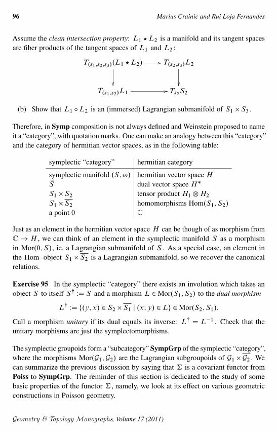
96 Marius Crainic and Rui Loja Fernandes
Assume the clean intersection property: L1 ?L2 is a manifold and its tangent spacesare fiber products of the tangent spaces of L1 and L2 :
T.s1;s2;s3/.L1 ?L2/ //
��
T.s2;s3/L2
��T.s1;s2/L1
// Ts2S2
(b) Show that L1 ıL2 is an (immersed) Lagrangian submanifold of S1 �S3 .
Therefore, in Symp composition is not always defined and Weinstein proposed to nameit a “category”, with quotation marks. One can make an analogy between this “category”and the category of hermitian vector spaces, as in the following table:
symplectic “category” hermitian category
symplectic manifold .S; !/ hermitian vector space HxS dual vector space H�
S1 �S2 tensor product H1˝H2
S1 �S2 homomorphisms Hom.S1;S2/
a point 0 C
Just as an element in the hermitian vector space H can be though of as morphism fromC ! H , we can think of an element in the symplectic manifold S as a morphismin Mor.0;S/, ie, a Lagrangian submanifold of S . As a special case, an element inthe Hom–object S1 �S2 is a Lagrangian submanifold, so we recover the canonicalrelations.
Exercise 95 In the symplectic “category” there exists an involution which takes anobject S to itself S| WD S and a morphism L 2Mor.S1;S2/ to the dual morphism
L|WD f.y;x/ 2 S2 �S1 j .x;y/ 2Lg 2Mor.S2;S1/:
Call a morphism unitary if its dual equals its inverse: L| D L�1 . Check that theunitary morphisms are just the symplectomorphisms.
The symplectic groupoids form a “subcategory” SympGrp of the symplectic “category”,where the morphisms Mor.G1;G2/ are the Lagrangian subgroupoids of G1 �G2 . Wecan summarize the previous discussion by saying that † is a covariant functor fromPoiss to SympGrp. The reminder of this section is dedicated to the study of somebasic properties of the functor †, namely, we look at its effect on various geometricconstructions in Poisson geometry.
Geometry & Topology Monographs, Volume 17 (2011)
Lectures on integrability of Lie brackets 97
Subobjects A subobject in the Poisson category is just a Poisson submanifold N ofa Poisson manifold .M; �/. As the following example shows, a Poisson submanifoldof an integrable Poisson manifold may fail to be integrable.
Example 5.27 Let M D so.4/� with its linear Poisson structure. Note that we havean isomorphism
so.4/' so.3/˚ so.3/D su.2/˚ su.2/;
so that we can think of M as R6DR3�R3 with the product Poisson structure, whereeach factor has the Poisson structure (5.20). For the usual Euclidean structure on R6 ,the function f .x/D kxk2 is a Casimir, so that the unit sphere
S5D fx 2R6
W kxk D 1g;
is a Poisson submanifold of M .
Exercise 96 Determine which points of S5 are regular points. Using Proposition 5.4,show that if x D .x1;x2/ 2 S5 is a regular point then:
Nx ' fn1kx1kC n2kx2k W n1; n2 2 Zg �R:
Therefore, S5 is not an integrable Poisson manifold.
Henceforth, we will assume that both .M; �/ and the Poisson submanifold N areintegrable. Then the inclusion i W N ,!M is a Poisson morphism which, accordingto Corollary 5.25, integrates to a Lagrangian subgroupoid †.i/ � †.N / �†.M /.However, this is not the end of the story.
For a Poisson submanifold N �M , let us consider the set of equivalence classes ofcotangent paths that take their values in the restricted subbundle T �
NM :
†N .M / WD fŒa� 2†.M / j aW I ! T �N M g:
This is a Lie subgroupoid of †.M /: it is the Lie subgroupoid that integrates the Liesubalgebroid T �
NM �T �M . Moreover, this subalgebroid is a coisotropic submanifold
of the symplectic manifold T �M , and it follows that †N .M /�†.M / is a coisotropicLie subgroupoid. The fact that the closed 2–form ! on †N .M / is multiplicativeimplies that if we factor by its kernel foliation, we still obtain a symplectic groupoid,and in fact (see [15]):
†.N /'†N .M /=Ker!:
These two constructions are related as follows:
Geometry & Topology Monographs, Volume 17 (2011)
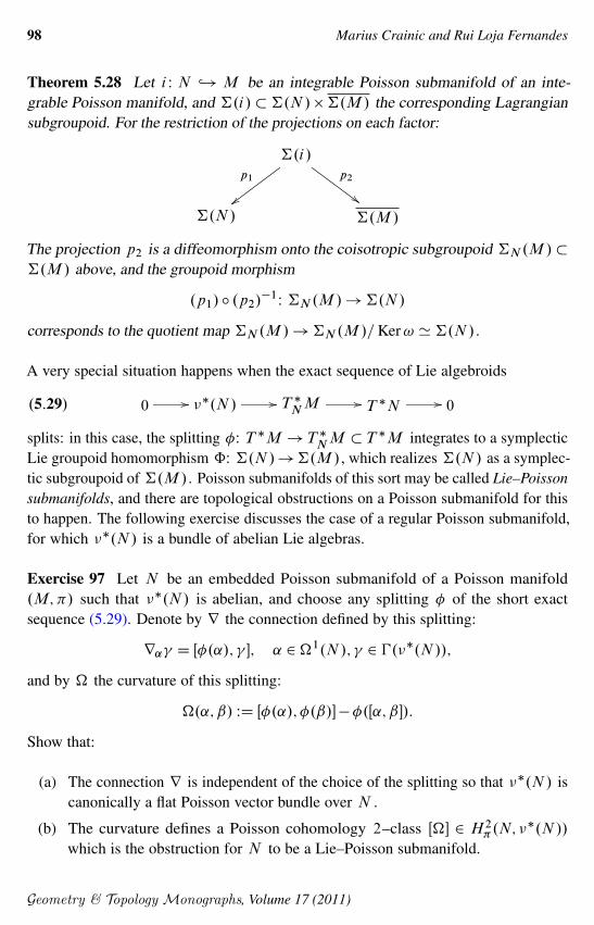
98 Marius Crainic and Rui Loja Fernandes
Theorem 5.28 Let i W N ,! M be an integrable Poisson submanifold of an inte-grable Poisson manifold, and †.i/�†.N /�†.M / the corresponding Lagrangiansubgroupoid. For the restriction of the projections on each factor:
†.i/
p1
{{
p2
##†.N / †.M /
The projection p2 is a diffeomorphism onto the coisotropic subgroupoid †N .M /�
†.M / above, and the groupoid morphism
.p1/ ı .p2/�1W †N .M /!†.N /
corresponds to the quotient map †N .M /!†N .M /=Ker! '†.N /.
A very special situation happens when the exact sequence of Lie algebroids
.5:29/ 0 // ��.N / // T �N
M // T �N // 0
splits: in this case, the splitting �W T �M ! T �N
M � T �M integrates to a symplecticLie groupoid homomorphism ˆW †.N /!†.M /, which realizes †.N / as a symplec-tic subgroupoid of †.M /. Poisson submanifolds of this sort may be called Lie–Poissonsubmanifolds, and there are topological obstructions on a Poisson submanifold for thisto happen. The following exercise discusses the case of a regular Poisson submanifold,for which ��.N / is a bundle of abelian Lie algebras.
Exercise 97 Let N be an embedded Poisson submanifold of a Poisson manifold.M; �/ such that ��.N / is abelian, and choose any splitting � of the short exactsequence (5.29). Denote by r the connection defined by this splitting:
r˛ D Œ�.˛/; �; ˛ 2�1.N /; 2 �.��.N //;
and by � the curvature of this splitting:
�.˛; ˇ/ WD Œ�.˛/; �.ˇ/���.Œ˛; ˇ�/:
Show that:
(a) The connection r is independent of the choice of the splitting so that ��.N / iscanonically a flat Poisson vector bundle over N .
(b) The curvature defines a Poisson cohomology 2–class Œ�� 2 H 2�.N; �
�.N //
which is the obstruction for N to be a Lie–Poisson submanifold.
Geometry & Topology Monographs, Volume 17 (2011)

Lectures on integrability of Lie brackets 99
(c) If N is a Lie–Poisson submanifold, then N is integrable.
(d) If N is simply connected, then N is a Lie–Poisson submanifold if and only ifits monodromy group vanishes.
Quotients What we have just seen for subobjects is typical: though the functor †gives us some indication of what the integration of a certain geometric construction is,there is often extra geometry hidden in the symplectization. Another instance of thishappens when one looks at quotients.
Let G be a Lie group that acts smoothly by Poisson diffeomorphisms on a Poissonmanifold .M; �/. We will denote the action by ‰W G �M !M and we will alsowrite ‰.g;x/D g �x . For each g 2G , we set
‰gW M !M; x 7! g �x;
so that each ‰g is a Poisson diffeomorphism.
Now we apply the functor †. For each g 2G , we obtain a Lagrangian subgroupoid†.‰g/ � †.M / � †.M /. This Lagrangian subgroupoid is, in fact, the graph ofa symplectic Lie groupoid automorphism, which we denote by the same symbol†.‰g/W †.M /!†.M /. Also, it is not hard to check that
†.‰/W G �†.M /!†.M /; .g; Œa�/ 7! g � Œa� WD†.‰g/.Œa�/;
defines a symplectic smooth action of G on †.M /. Briefly, † lifts a Poisson action‰W G �M !M to a symplectic action †.‰/W G �†.M /! †.M / by groupoidautomorphisms. However, this is not the end of the story.
Let us look closer at how one lifts the action from M to †.M /. First of all, recall thatany smooth action G �M !M has a lifted cotangent action G �T �M ! T �M .This yields, by composition, an action of G on cotangent paths: if aW I ! T �M is acotangent path we just move it around
.g � a/.t/ WD g � a.t/:
The fact that the original action G �M ! M is Poisson yields that (i) g � a is acotangent path whenever a is a cotangent path, and (ii) if a0 and a1 are cotangenthomotopic then so are the translated paths g � a0 and g � a1 . Therefore, we have awell-defined action of G on cotangent homotopy classes and this is just the liftedaction: †.‰g/.Œa�/D Œg � a�.
Now we invoke a simple (but important) fact from symplectic geometry: for any actionG �M !M the lifted cotangent action G �T �M ! T �M is a Hamiltonian action
Geometry & Topology Monographs, Volume 17 (2011)

100 Marius Crainic and Rui Loja Fernandes
with equivariant momentum map j W T �M ! g� given by
j W T �M ! g�; hj .˛x/; �i WD h˛x;X�.x/i;
where X� 2 X.M / is the infinitesimal generator associated with � 2 g. This yieldsimmediately the fact that the lifted action †.‰/W G �†.M /!†.M / is also Hamil-tonian12 with equivariant momentum map J W †.M /! g� is given by
.5:30/ hJ.Œa�/; �i WD
Z 1
0
j .a.t// dt D
Za
X� :
Since each X� is a Poisson vector field, the last expression shows that only the cotangenthomotopy class of a matters, and J is indeed well-defined. Expression (5.30) meansthat we can see the momentum map of the †.‰/–action in two ways:
� It is the integration of the momentum map of the lifted cotangent action.� It is the integration of the infinitesimal generators along cotangent paths.
In any case, expression (5.30) for the momentum map shows that it satisfies thefollowing additive property:
J.Œa0� � Œa1�/D J.Œa0�/CJ.Œa1�/:
Hence J is a groupoid homomorphism from †.M / to the additive group .g�;C/ or,which is the same, J is differentiable groupoid 1–cocycle. Moreover, this cocycle isexact if and only if there exists a map �W M ! g� such that
J D � ı t�� ı s;
and this happens precisely if and only if the original Poisson action ‰W G �M !M
is Hamiltonian with equivariant momentum map �W M ! g� . We summarize all thisin the following theorem:
Theorem 5.31 Let ‰W G �M ! M be a smooth action of a Lie group G ona Poisson manifold M by Poisson diffeomorphisms. There exists a lifted action†.‰/W G �†.M /!†.M / by symplectic groupoid automorphisms. This lifted G –action is Hamiltonian and admits the momentum map J W †.M /! g� given by (5.30).Furthermore:
(i) The momentum map J is G –equivariant and is a groupoid 1–cocycle.
(ii) The G–action on M is Hamiltonian with momentum map �W M ! g� if andonly if J is an exact cocycle.
12Recall again that, after all, the symplectic structure on †.M / comes from canonical symplecticstructures on cotangent bundles.
Geometry & Topology Monographs, Volume 17 (2011)

Lectures on integrability of Lie brackets 101
Let us now assume that the Poisson action ‰W G �M !M is proper and free. Theseassumptions guarantee that M=G is a smooth manifold. The space C1.M=G/ ofsmooth functions on the quotient is naturally identified with the space C1.M /G ofG–invariant functions on M . Since the Poisson bracket of G–invariant functions isa G–invariant function, we have a quotient Poisson structure on M=G such that thenatural projection M !M=G is a Poisson map.
Exercise 98 Show that if .M; �/ is an integrable Poisson structure and ‰W G�M !
M is proper and free Poisson action, then M=G is also an integrable Poisson manifold.
So the question arises: what is the relationship between the symplectic groupoids†.M / and †.M=G/?
First notice that if the original Poisson action ‰W G �M !M is proper and free, sois the lifted action †.‰/W G �†.M /!†.M /. Therefore 0 2 g� is a regular valueof the momentum map J W †.M /! g� . Let us look at the symplectic quotient:
†.M /==G WD J�1.0/=G:
Since J is a groupoid homomorphism, its kernel J�1.0/�†.M / is a Lie subgroupoid.Since J is G –equivariant, the action leaves J�1.0/ invariant and the restricted actionis a free action by groupoid automorphisms. Hence, the groupoid structure descends toa groupoid structure †.M /==G�M=G .
Exercise 99 Show that †.M /==G is a symplectic groupoid that integrates the quotientPoisson manifold M=G .
In general, however, it is not true that
†.M=G/D†.M /==G;
so, in general, symplectization does not commute with reduction. First of all, J�1.0/
may be nonconnected, so that †.M /==G may have nonconnected source fibers. Evenif we restrict to J�1.0/c , the connected component of the identity section (so thatthe source fibers of †.M /==G are connected) these fibers may have a nontrivialfundamental group, as shown by the following exercise:
Exercise 100 Consider the proper and free action of S1 on M D C2 � f0g thatis given by � � .z1; z2/ D .ei�z1; e
�i�z2/. For the canonical symplectic structure! D .i=2/.dz1 ^ dxz1C dz2 ^ dxz2/, this S1 –action on M is Poisson. Determine bothgroupoids †.M /==G and †.M=G/ and show that they are not isomorphic.
We will not get here into the subtleties of this problem.
Geometry & Topology Monographs, Volume 17 (2011)

102 Marius Crainic and Rui Loja Fernandes
5.5 Notes
The notion of a symplectic groupoid and its relation to Poisson geometry appears first inWeinstein [56] and is discuss in greater detail in Coste, Dazord and Weinstein [12]. Theintegration of Poisson manifolds presented here has its roots in the work of Cattaneoand Felder [8] on the Poisson sigma model and was discussed first by us in [16].
The main positive integrability result of [8] states that any Poisson structure on R2
is integrable. This is also a consequence of a general result due to Debord [17] (seealso [15, Corollary 5.9]) that states that a Lie algebroid with almost injective anchor isintegrable. The results on the integrability of regular Poisson manifolds and its relationto the variation of symplectic areas are due to Alcade-Cuesta and Hector [1]. Thetwo examples we presented (the modified su�.2/–bracket and the Heisenberg–Poissonmanifolds) are both due to Weinstein [56; 58].
The “symplectic category” appears early in the modern history of symplectic geometryand is due to Weinstein [55]. Also, in his first note on symplectic groupoids heobserves that a Poisson morphism integrates to a canonical relation. Coisotropicsubmanifolds are first studied in a systematic way by Weinstein in [57], in connectionwith Poisson groupoids. The problem of integrating coisotropic submanifolds wassolved by Cattaneo and Felder in [9]. The integration of Poisson submanifolds (andmore general submanifolds) was discussed first by Xu in [63] and then completed byus in [16]. Actions of groups on groupoids, and some of the properties on lifted actionscan be found, in one form or another, in Condevaux, Dazord and Molino [10], Coste,Dazord and Weinstein [12], Mikami and Weinstein [40], Weinstein and Xu [60] andXu [61]. This problem, including the case of nonfree actions and Poisson–Lie groupsis also discussed by Fernandes, Ortega and Ratiu [26] and Fernandes and IglesiasPonte [25].
The symplectization functor can be (and should be!) applied to many other constructionsin Poisson geometry. For example, one can look at the symplectization of Poissonfibrations (in the sense of Vorobjev [54]) and this yields groupoids which are symplecticfibrations (in the sense of Guillemin, Lerman and Sternberg [29] and McDuff andSalamon [39]). Another example, is provided by the connected sum constructionin Poisson geometry (see Ibort and Martínez Torres [33]) which out of two Poissonmanifolds M1 and M2 yields, under some conditions, a new Poisson manifold M1#M2 .A result of the sort
†.M1#M2/D†.M1/#†.M2/
should be true (here, on the right-hand side one has a symplectic connected sum). Athird example, is in the theory of Poisson–Nijenhuis manifolds where the application
Geometry & Topology Monographs, Volume 17 (2011)
Lectures on integrability of Lie brackets 103
of the † functor leads to a symplectic-Nijenhuis groupoid (see Crainic [13]), and thisis relevant both in the study of the generalized complex structures and of integrablehierarchies associated with a PN–manifold. The symplectization functor †, which wehave just started understanding, should play an important role in many other problemsin Poisson geometry.
References[1] F Alcalde-Cuesta, G Hector, Intégration symplectique des variétés de Poisson
régulières, Israel J. Math. 90 (1995) 125–165 MR1336320
[2] R Almeida, P Molino, Suites d’Atiyah et feuilletages transversalement complets, C. R.Acad. Sci. Paris Sér. I Math. 300 (1985) 13–15 MR778785
[3] K Behrend, L Fantechi, W Fulton, L Goettsche, A Kresch, An introduction to stacks,Book in preparation
[4] K Behrend, P Xu, Differentiable stacks and gerbes arXiv:math.DG/0605694
[5] W Brandt, Über eine Verallgemeinerung des Gruppenbegriffes, Math. Ann. 96 (1926)360–366
[6] R L Bryant, Bochner-Kähler metrics, J. Amer. Math. Soc. 14 (2001) 623–715MR1824987
[7] É Cartan, Sur la structure des groupes infinis de transformation, Ann. Sci. École Norm.Sup. (3) 21 (1904) 153–206 MR1509040
[8] A S Cattaneo, G Felder, Poisson sigma models and symplectic groupoids, from:“Quantization of singular symplectic quotients”, (N P Landsman, M Pflaum, MSchlichenmaier, editors), Progr. Math. 198, Birkhäuser, Basel (2001) 61–93MR1938552
[9] A S Cattaneo, G Felder, Coisotropic submanifolds in Poisson geometry and branes inthe Poisson sigma model, Lett. Math. Phys. 69 (2004) 157–175 MR2104442
[10] M Condevaux, P Dazord, P Molino, Géométrie du moment, from: “Travaux duSéminaire Sud-Rhodanien de Géométrie, I”, Publ. Dép. Math. Nouvelle Sér. B 88, Univ.Claude-Bernard, Lyon (1988) 131–160 MR1040871
[11] A Connes, Noncommutative geometry, Academic Press, San Diego (1994)MR1303779
[12] A Coste, P Dazord, A Weinstein, Groupoïdes symplectiques, from: “Publications duDépartement de Mathématiques. Nouvelle Série. A, Vol. 2”, Publ. Dép. Math. NouvelleSér. A 87, Univ. Claude-Bernard, Lyon (1987) i–ii, 1–62 MR996653
[13] M Crainic, Generalized complex structures and Lie brackets arXiv:math.DG/0412097
Geometry & Topology Monographs, Volume 17 (2011)

104 Marius Crainic and Rui Loja Fernandes
[14] M Crainic, Differentiable and algebroid cohomology, van Est isomorphisms, andcharacteristic classes, Comment. Math. Helv. 78 (2003) 681–721 MR2016690
[15] M Crainic, R L Fernandes, Integrability of Lie brackets, Ann. of Math. .2/ 157 (2003)575–620 MR1973056
[16] M Crainic, R L Fernandes, Integrability of Poisson brackets, J. Differential Geom. 66(2004) 71–137 MR2128714
[17] C Debord, Feuilletages singulaires et groupoïdes d’holonomie, PhD thesis, UniversitéPaul Sabatier, Toulouse (2000)
[18] A Douady, M Lazard, Espaces fibrés en algèbres de Lie et en groupes, Invent. Math.1 (1966) 133–151 MR0197622
[19] J-P Dufour, N T Zung, Poisson structures and their normal forms, Progress in Math.242, Birkhäuser Verlag, Basel (2005) MR2178041
[20] J J Duistermaat, J A C Kolk, Lie groups, Universitext, Springer, Berlin (2000)MR1738431
[21] C Ehresmann, Œuvres complètes et commentées. I-1,2. Topologie algébrique etgéométrie différentielle, Cahiers Topologie Géom. Différentielle 24 (1983) MR794193
[22] S Evens, J-H Lu, A Weinstein, Transverse measures, the modular class and a coho-mology pairing for Lie algebroids, Quart. J. Math. Oxford Ser. .2/ 50 (1999) 417–436MR1726784
[23] R L Fernandes, Connections in Poisson geometry. I. Holonomy and invariants, J.Differential Geom. 54 (2000) 303–365 MR1818181
[24] R L Fernandes, Lie algebroids, holonomy and characteristic classes, Adv. Math. 170(2002) 119–179 MR1929305
[25] R L Fernandes, D Iglesias Ponte, Integrability of Poisson–Lie group actions, Lett.Math. Phys. 90 (2009) 137–159 MR2565037
[26] R L Fernandes, J-P Ortega, T S Ratiu, The momentum map in Poisson geometry,Amer. J. Math. 131 (2009) 1261–1310 MR2555841
[27] V L Ginzburg, Grothendieck groups of Poisson vector bundles, J. Symplectic Geom. 1(2001) 121–169 MR1959580
[28] A Grothendieck, Techniques de construction en géométrie analytique I–X, from:“Familles d’espaces complexes et fondements de la géométrie analytique”, SéminaireHenri Cartan 1960/61, Exp. 7–17, Secrétariat mathématique, Paris (1962)
[29] V Guillemin, E Lerman, S Sternberg, Symplectic fibrations and multiplicity diagrams,Cambridge Univ. Press (1996) MR1414677
[30] A Haefliger, Homotopy and integrability, from: “Manifolds–Amsterdam 1970 (Proc.Nuffic Summer School)”, Lecture Notes in Math. 197, Springer, Berlin (1971) 133–163MR0285027
Geometry & Topology Monographs, Volume 17 (2011)

Lectures on integrability of Lie brackets 105
[31] P J Higgins, K C H Mackenzie, Algebraic constructions in the category of Lie alge-broids, J. Algebra 129 (1990) 194–230 MR1037400
[32] J Huebschmann, Duality for Lie–Rinehart algebras and the modular class, J. ReineAngew. Math. 510 (1999) 103–159 MR1696093
[33] A Ibort, D Martínez Torres, A new construction of Poisson manifolds, J. SymplecticGeom. 2 (2003) 83–107 MR2128389
[34] M V Karasëv, Analogues of objects of the theory of Lie groups for nonlinear Poissonbrackets, Izv. Akad. Nauk SSSR Ser. Mat. 50 (1986) 508–538, 638 MR854594
[35] A Kumpera, D Spencer, Lie equations. Vol. I: General theory, Annals of Math. Studies73, Princeton Univ. Press (1972) MR0380908
[36] K C H Mackenzie, Lie groupoids and Lie algebroids in differential geometry, LondonMath. Soc. Lecture Note Ser. 124, Cambridge Univ. Press (1987) MR896907
[37] K C H Mackenzie, Lie algebroids and Lie pseudoalgebras, Bull. London Math. Soc.27 (1995) 97–147 MR1325261
[38] K C H Mackenzie, General theory of Lie groupoids and Lie algebroids, London Math.Soc. Lecture Note Ser. 213, Cambridge Univ. Press (2005) MR2157566
[39] D McDuff, D Salamon, Introduction to symplectic topology, second edition, Ox-ford Math. Monogr., The Clarendon Press, Oxford Univ. Press, New York (1998)MR1698616
[40] K Mikami, A Weinstein, Moments and reduction for symplectic groupoids, Publ. Res.Inst. Math. Sci. 24 (1988) 121–140 MR944869
[41] I Moerdijk, Orbifolds as groupoids: an introduction, from: “Orbifolds in mathematicsand physics (Madison, WI, 2001)”, (A Adem, J Morava, Y Ruan, editors), Contemp.Math. 310, Amer. Math. Soc. (2002) 205–222 MR1950948
[42] I Moerdijk, J Mrcun, On integrability of infinitesimal actions, Amer. J. Math. 124(2002) 567–593 MR1902889
[43] I Moerdijk, J Mrcun, Introduction to foliations and Lie groupoids, Cambridge Studiesin Advanced Math. 91, Cambridge Univ. Press (2003) MR2012261
[44] V Nistor, Groupoids and the integration of Lie algebroids, J. Math. Soc. Japan 52(2000) 847–868 MR1774632
[45] R S Palais, A global formulation of the Lie theory of transformation groups, Mem.Amer. Math. Soc. 22 (1957) MR0121424
[46] J Pradines, Théorie de Lie pour les groupoïdes différentiables. Relations entre pro-priétés locales et globales, C. R. Acad. Sci. Paris Sér. A-B 263 (1966) A907–A910MR0214103
Geometry & Topology Monographs, Volume 17 (2011)

106 Marius Crainic and Rui Loja Fernandes
[47] J Pradines, Théorie de Lie pour les groupoïdes différentiables. Calcul différenetieldans la catégorie des groupoïdes infinitésimaux, C. R. Acad. Sci. Paris Sér. A-B 264(1967) A245–A248 MR0216409
[48] J Pradines, Géométrie différentielle au-dessus d’un groupoïde, C. R. Acad. Sci. ParisSér. A-B 266 (1968) A1194–A1196 MR0231306
[49] J Pradines, Troisième théorème de Lie les groupoïdes différentiables, C. R. Acad. Sci.Paris Sér. A-B 267 (1968) A21–A23 MR0231414
[50] P Ševera, Some title containing the words “homotopy” and “symplectic”, eg this one,Trav. Math. XVI, Univ. Luxemb. (2005) 121–137 MR2223155
[51] A Cannas da Silva, A Weinstein, Geometric models for noncommutative algebras,Berkeley Math. Lecture Notes 10, Amer. Math. Soc. (1999) MR1747916
[52] I M Singer, S Sternberg, The infinite groups of Lie and Cartan. I. The transitive groups,J. Analyse Math. 15 (1965) 1–114 MR0217822
[53] A Y Vaıntrob, Lie algebroids and homological vector fields, Uspekhi Mat. Nauk 52(1997) 161–162 MR1480150
[54] Y Vorobjev, Coupling tensors and Poisson geometry near a single symplectic leaf,from: “Lie algebroids and related topics in differential geometry (Warsaw, 2000)”, (JKubarski, P Urbanski, R Wolak, editors), Banach Center Publ. 54, Polish Acad. Sci.,Warsaw (2001) 249–274 MR1881658
[55] A Weinstein, Symplectic geometry, Bull. Amer. Math. Soc. .N.S./ 5 (1981) 1–13MR614310
[56] A Weinstein, Symplectic groupoids and Poisson manifolds, Bull. Amer. Math. Soc..N.S./ 16 (1987) 101–104 MR866024
[57] A Weinstein, Coisotropic calculus and Poisson groupoids, J. Math. Soc. Japan 40(1988) 705–727 MR959095
[58] A Weinstein, Blowing up realizations of Heisenberg–Poisson manifolds, Bull. Sci.Math. 113 (1989) 381–406 MR1029617
[59] A Weinstein, Linearization of regular proper groupoids, J. Inst. Math. Jussieu 1 (2002)493–511 MR1956059
[60] A Weinstein, P Xu, Extensions of symplectic groupoids and quantization, J. ReineAngew. Math. 417 (1991) 159–189 MR1103911
[61] P Xu, Symplectic groupoids of reduced Poisson spaces, C. R. Acad. Sci. Paris Sér. IMath. 314 (1992) 457–461 MR1154386
[62] P Xu, Gerstenhaber algebras and BV-algebras in Poisson geometry, Comm. Math.Phys. 200 (1999) 545–560 MR1675117
[63] P Xu, Dirac submanifolds and Poisson involutions, Ann. Sci. École Norm. Sup. .4/ 36(2003) 403–430 MR1977824
Geometry & Topology Monographs, Volume 17 (2011)

Lectures on integrability of Lie brackets 107
[64] J A Yorke, Periods of periodic solutions and the Lipschitz constant, Proc. Amer. Math.Soc. 22 (1969) 509–512 MR0245916
[65] S Zakrzewski, Quantum and classical pseudogroups. I. Union pseudogroups and theirquantization, Comm. Math. Phys. 134 (1990) 347–370 MR1081010
[66] N T Zung, Proper groupoids and momentum maps: linearization, affinity, and convexity,Ann. Sci. École Norm. Sup. .4/ 39 (2006) 841–869 MR2292634
Department of Mathematics, Utrecht University3508 TA Utrecht, The Netherlands
Departamento de Matemática, Instituto Superior Técnico1049-001 Lisboa, Portugal
[email protected], [email protected]
http://www.math.uu.nl/people/crainic/
Received: 18 May 2010
Geometry & Topology Monographs, Volume 17 (2011)