Lectures on Hybrid Logic

NASSLLI’02, First North American Summer School in Logic, Language,and Information, 24–28 June 2002, Stanford

Patrick Blackburn Maarten MarxINRIA, Lorraine University of Amsterdampatrick@aplog.org marx@science.uva.nl

This course introduces hybrid logic, a form of modal logic in which it is possible toname worlds (or times, or computational states, or situations, or nodes in parse trees, orpeople — indeed, whatever it is that the elements of Kripke Models are taken to represent).The course has two main goals. The first is to convey, as clearly as possible, the ideasand intuitions that have guided the development of hybrid logic. The second is to teacha concrete skill: tableau-based hybrid deduction. By the end of the course you will haveample evidence that modal logic can be useful in a wide range of circumstances, and thathybrid logic is a particularly simple way of doing modal logic.

Course Outline

The course consist of five lectures:

Lecture 1: From modal logic to hybrid logic

Lecture 2: Hybrid deduction

Lecture 3: The downarrow binder

Lecture 4: First-order hybrid logic

Lecture 5: The Priorean perspective

Each lecture is one hour long, and will be presented by Patrick Blackburn. The slides(developed by Patrick Blackburn and Maarten Marx) on which the course is basedwill be made available on the NASSLLI website, and on the hybrid logic homepage(www.hylo.net).

The course is relatively self-contained, and we attempt to make the material as ac-cessible as possible to an interdisciplinary audience (that is, the course is not targetedsolely at logicians). Nonetheless, we presuppose a certain level of logical literacy. Roughlyspeaking, to follow this course you should have a reasonable grasp of first-order logic andits semantics. Prior acquaintance with the basics of modal logic would be helpful, but isnot essential.

This Reader

This reader consist of three papers:

• “Representation, Reasoning, and Relational Structures: a Hybrid Logic Manifesto”,by Patrick Blackburn. Logic Journal of the IGPL, 8(3), 339-625, 2000.

• “Tableaux for Quantified Hybrid Logic” by Patrick Blackburn and Maarten Marx,to appear in Proceedings of Tableaux 2002, Automated Reasoning with AnalyticTableaux and Related Methods, Copenhagen, Denmark, July 30th – August 1st,2002.

• “Beyond Pure Axioms: Node Creating Rules in Hybrid Tableaux” by Patrick Black-burn and Balder ten Cate. Draft manuscript, 2002.

1

These papers are intended to act as background reading: they should help you under-stand the themes discussed in class better, and in some cases they develop these themesfurther, or in different directions.

The “Manifesto” provides an intuitive overview of the full range of (non first-order)hybrid logics, and explains the basics of hybrid tableaux for various hybrid language. Itis central to the course, providing background to Lectures 1, 2, 3 and 5.

However the manifesto does not discuss first-order hybrid logic, the topic of Lecture 4.To fill this gap we have supplied “Tableaux for Quantified Hybrid Logic”. We have delib-erately chosen a paper in which the approach to first-order hybrid logic is slightly differentfrom that which will be discussed in class. In Lecture 4 we present first-order hybrid logicunder the varying-domain semantics. This paper, on the other hand, uses the (somewhatsimpler) constant domain semantics. One of the pleasant aspects of hybrid logic is thateither approach works smoothly, and the reader will find it interesting to compare thepaper with the course slides. One other remark: modal logicians will find the complete-ness proof in this paper novel. Instead of using a traditional Henkin- or Hintikka-styleargument, completeness is proved by a translation from first-order logic. Non logiciansmay find this part of the paper tough going.

Finally, the “Beyond Pure Axioms” paper will give you a taste of some recent work inhybrid deduction. Essentially, this paper shows that the results discussed in class aboutpure axioms can be extended to yield deduction systems for a far wider class of logics.Moreover, the paper also makes use of the strong Priorean-style hybrid language discussedin Lecture 5 to characterise these logics. In addition, the paper’s appendix shows howto prove the completeness of a hybrid tableaux system using a traditional Hintikka-styleargument. All in all, a nice way of rounding off various themes discussed in the course.

Acknowledgements

We would like to thank INRIA, France’s national research organization in computer sci-ence, who provided financial support for this course as part of the INRIA-funded re-search collaboration between the Langue et Dialogue group (INRIA Lorraine, Nancy)and the Language and Inference Technology group (University of Amsterdam); seehttp://www.loria.fr/projets/ledcalg. The course material was developed during anINRIA-funded visit by Maarten Marx to Langue et Dialogue. We would also like to thankCarlos Areces, Torben Brauner, Balder ten Cate, and Eric Kow for helping out in variousways in the run-up to NASSLLI.

2

Representation, Reasoning, andRelational Structures: a Hybrid Logic Manifesto

Patrick BlackburnINRIA Lorraine, Nancy, France

patrick@aplog.org

Abstract

This paper is about the good side of modal logic, the bad side of modal logic, andhow hybrid logic takes the good and fixes the bad.

In essence, modal logic is a simple formalism for working with relational structures(or multigraphs). But modal logic has no mechanism for referring to or reasoningabout the individual nodes in such structures, and this lessens its effectiveness as arepresentation formalism. In their simplest form, hybrid logics are upgraded modallogics in which reference to individual nodes is possible.

But hybrid logic is a rather unusual modal upgrade. It pushes one simple idea asfar as it will go: represent all information as formulas. This turns out to be the keyneeded to draw together a surprisingly diverse range of work (for example, featurelogic, description logic and labelled deduction). Moreover, it displays a number ofknowledge representation issues in a new light, notably the importance of sorting.

Keywords Labelled Deduction, Description Logic, Feature Logic, Hybrid Logic,Modal Logic, Sorted Modal Logic, Temporal Logic, Nominals, Knowledge Represen-tation, Relational Structures

1 Modal logic and relational structures

To get the ball rolling, let’s recall the syntax and semantics of (propositional) multimodallogic.

Definition 1 (Multimodal languages) Given a set of propositional symbols PROP ={p, q, p′, q′, . . .}, and a set of modality labels MOD = {π, π′, . . .}, the set of well-formed formulasof the multimodal language (over PROP and MOD) is defined as follows:

WFF := p | ¬ϕ | ϕ ∧ ψ | ϕ ∨ ψ | ϕ→ ψ | 〈π〉ϕ | [π]ϕ,

for all p ∈ PROP and π ∈ MOD. As usual, ϕ↔ ψ := (ϕ→ ψ) ∧ (ψ → ϕ).

Definition 2 ((Kripke) models) Such a language is interpreted on models (often called

Kripke models). A model M (for a fixed choice of PROP and MOD) is a triple (W, {Rπ |π ∈ MOD}, V ). Here W is a non-empty set (I’ll call its elements states, or nodes), and each Rπ

is a binary relations on W . The pair (W, {Rπ | π ∈ MOD}) is called the frame underlying M,

and M is said to be a model based on this frame. V (the valuation) is a function with domain

PROP and range Pow(W ); it tells us at which states (if any) each propositional symbol is true.

Definition 3 (Satisfaction and validity) Interpretation is carried out using the Kripkesatisfaction definition. Let M = (W, {Rπ | π ∈ MOD}, V ) and w ∈W . Then:

M, w p iff w ∈ V (p), where p ∈ PROPM, w ¬ϕ iff M, w 6 ϕM, w ϕ ∧ ψ iff M, w ϕ and M, w ψM, w ϕ ∨ ψ iff M, w ϕ or M, w ψM, w ϕ→ ψ iff M, w 6 ϕ or M, w ψM, w 〈π〉ϕ iff ∃w′(wRπw

′ & M, w′ ϕ)M, w [π]ϕ iff ∀w′(wRπw

′ ⇒ M, w′ ϕ).

IfM, w ϕ we say that ϕ is satisfied inM at w. If ϕ is satisfied at all states in all models based

on a frame F , then we say that ϕ is valid on F and write F ϕ. If ϕ is valid on all frames,

then we say that it is valid and write ϕ.

Now, you’ve certainly seen these definitions before — but if you want to understandcontemporary modal logic you need to think about them in a certain way. Above all, pleasedon’t automatically think of models as a collection of “worlds” together with various “ac-cessibility relations between worlds”, and don’t think of modalities as “non-classical logical

3

symbols” suitable only for coping with intensional concepts such as necessity, possibility,and belief. Modal logic can be viewed in these terms, but it’s a rather limited perspective.Instead, think of models as relational structures, or multigraphs. That is, think of a modelas an underlying set together with a collection of binary and unary relations. We use themodalities to talk about the binary relations, and the propositional symbols to talk aboutthe unary relations.

Remark 1 (Kripke models are relational structures) Let’s make this precise. Con-

sider a model M = (W, {Rπ | π ∈ MOD}, V ). The underlying frame (W, {Rπ | π ∈ MOD})is already presented in explicitly relational terms, and it is trivial to present the information

in the valuation in same way: in fact M can be presented as the following relational structure

M = (W, {Rπ | π ∈ MOD}, {V (p) | p ∈ PROP}).

Why think in terms of relational structures? Two reasons. The first is: relationalstructures are ubiquitous. Virtually all standard mathematical structures can be viewedas relational structures, as can inheritance hierarchies, transition systems, parse trees,and other structures used in AI, computer science, and computational linguistics. Indeed,anytime you draw a diagram consisting of nodes, arcs, and labels, you have drawn somekind of relational structure. There are no preset limits to the applicability of modal logic:as it is a tool for talking about relational structures, it can be applied just about anywhere.

Secondly, relational structures are the models of classical model theory (see, for exam-ple, Hodges [35]). Thus there is nothing intrinsically “modal” about Kripke models, andwe’re certainly not forced to talk about them using modal languages. On the contrary,we can talk about models using any classical language we find useful (for example, afirst-order, infinitary, fixpoint, or second-order language). Unsurprisingly, this means thatmodal and classical logic are systematically related.

Remark 2 (Modal logic is a fragment of classical logic) To talk about a Kripkemodel in a classical language, all we have to do is view it as a relational structure (as describedin the previous example) and then ‘read off’ from the signature (that is, MOD and PROP) thenon-logical symbols we need, namely a MOD-indexed collection of two place relation symbols Rπ,and a PROP-indexed collection of unary relation symbols P, Q, P′, Q′, and so on. We then buildformulas in the classical language of our choice.

As modal languages and classical languages both talk about relational structures, it seemsoverwhelmingly likely that a systematic relationship exists between them. And in fact, the modallanguage (over PROP and MOD) can be translated into the best-known classical language of all,namely the first-order language (over PROP and MOD). Here are some clauses of the StandardTranslation, a top-down translation which inductively maps modal to first-order formulas:

STx(p) = P(x), p ∈ PROPSTx(¬ϕ) = ¬STx(ϕ)STx(ϕ ∧ ψ) = STx(ϕ) ∧ STx(ψ)STx(〈π〉ϕ) = ∃y(xRπy ∧ STy(ϕ))STx([π]ϕ) = ∀y(xRπy → STy(ϕ))

Here x is a fixed but arbitrary free variable. In the fourth and fifth clause, the variable y canbe any variable not used so far in the translation. The clauses governing STy are analogous tothose given for STx; in particular, the clauses for the modalities introduce a new variable (say z)and so on. For any modal formula ϕ, STx(ϕ) is a first-order formula containing exactly one freevariable (namely x), and it is easy to see that M, w ϕ iff M |= STx(ϕ)[w] (where |= denotesthe first-order satisfaction relation and [w] means assign the state w to the free variable x inSTx(ϕ)). The equivalence can be proved by induction, but it should be self-evident: the StandardTranslation is simply a reformulation of the clauses of the Kripke satisfaction definition.

There are also non-trivial links between modal logic and infinitary logic, fixed-point logic,

and second-order logic; in particular, modal validity is intrinsically second-order. For further

discussion, see Blackburn, de Rijke, and Venema [14].

In short, modal logic is not some mysterious non-classical intensional logic, and modali-ties are not strange new devices. On the contrary, modalities are simply macros that handlequantification over accessible states.

This, of course, leads to another question. OK — so we can use modal logic whenworking with relational structures — but why bother if it’s really just a disguised way of

4

doing classical logic? I think the following two answers are the most important: modallogic brings simplicity and perspective.

Simplicity comes in a variety of forms. For a start, modal representations are oftenclean and compact: modalities pack a useful punch into a readable notation. Moreover,modal logic often brings us back to the realms of the computable: while the first-orderlogic over MOD and PROP is undecidable (whenever MOD is non-empty), its modal logicis decidable (in fact, PSPACE-complete).

Perspective is more subtle. Modal languages talk about relational structures in aspecial way: they take an internal and local perspective on relational structure. When weevaluate a modal formula, we place it inside, the model, at some particular state w (thecurrent state). The satisfaction clause (and in particular, the clause for the modalities)allow us to scan other states for information — but we’re only allowed to scan statesreachable from the current state. The reader should think of a modal formula as a littleautomaton, placed at some point on a graph, whose task is to explore the graph by visitingaccessible states. This internal, local, perspective is responsible for many of the attractivemathematical properties of modal logic. Moreover, it makes modal representations idealfor many applications. Here’s a classic example:

Example 1 (Temporal logic) We’ll be seeing a lot of the bimodal language with MOD ={F,P} in this paper: the modality F means “at some Future state”, and 〈P〉 means “at some Paststate”. To reflect this temporal interpretation, we usually interpret this language on frames of theform (T,<) that can plausibly be thought of as ‘flows of time’. For example, if we think of timeas a branching structure, (T,<) might be some kind of tree, and if we want a linear view of time,(T,<) might be (Z, <) (the integers in their usual order). When interpreting the language on suchframes we insist that RF is <, and RP is its converse; that is, as required, we ensure that F looksforward along the flow of time, and 〈P〉 backwards.

Consider the formula 〈P〉Mia-unconscious. This is true iff we can look back in time from thecurrent state and see a state where Mia is unconscious. Similarly FMia-unconscious requires usto scan the states that lie in the future looking for one where Mia is unconscious. Thus thesetwo formulas work similarly to the English sentences Mia has been unconscious and Mia will beunconscious: these sentences don’t specify an absolute time for Mia’s unconsciousness (which wecould do by giving a date and time), rather they locate it relative to the time of utterance. Inshort, English and other natural languages exploit the fact that human beings live in time, andmodal logic models this neatly.

This situated perspective can be lifted to more interesting temporal geometries. For exam-

ple, we could regard temporal states as unbroken intervals of time, add new modalities such as

〈SUB〉 (meaning “at some SUBinterval of the current state”) and 〈SUP〉 (meaning “at some

SUPerinterval of the current state”). Then a formula of the form 〈SUB〉F〈SUP〉p means “by

looking down to a subinterval, and then forward to the future, and then up to a superinterval, it

is possible to find a state where p is true”. Halpern and Shoham [34] take this idea to its ultimate

conclusion: abstracting from the work of James Allen [1], they present a modal logic which allows

all possible relationships between two closed intervals over a linear flow of time to be explored

‘from the inside’.

Nowadays, few modal logicians regard modal logic as a non-classical logic, and theycertainly don’t feel tied to any of the traditional interpretations of modal machinery.On the contrary, since the early 1970s modal logic has been explored as a subsystem ofvarious classical logics, and it is now clear that modal logic are a very special part ofclassical logic indeed. Indeed, modal languages are in many respects so natural, that —as modal logicians love to point out — it’s not particularly surprising that they havebeen independently reinvented by other research communities that make use of relationalstructures. Let’s look at two well known examples.

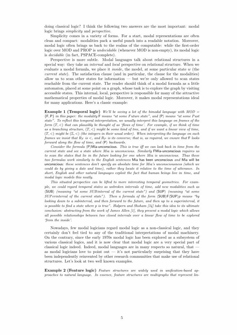
Example 2 (Feature logic) Feature structures are widely used in unification-based ap-proaches to natural language. In essence, feature structures are multigraphs that represent lin-

5

guistic information:

caseagreement

ss�

��

�/

@@

@@@R

numberperson

nominative

plural1st

ss�

��

�/

@@

@@@R

s

Computational linguists have a neat notation for talking about feature structures: Attribute-ValueMatrices (AVMs). Here’s an example: agreement

[person 1stnumber plural

]case −dative

This AVM is a partial description in the above feature structure — it’s satisfied in that structure atthe root node. The AVM describes a feature structure in which the agreement transition leadsto a node from which person and number transitions lead to the information 1st and pluralrespectively, and if you work down the left hand side of the previous diagram from the root you’llfind this structure. The AVM also demands a case transition from the root node that does notlead to the information dative. The feature structure depicted above also satisfies this requirement,for the case transition leads to a node bearing the information nominative.

Now, this all sounds very modal — and indeed, the AVM is a notational variant of the followingformula:

〈agreement〉(〈person〉1st ∧ 〈number〉plural)∧ 〈case〉¬dative

Example 3 (Description logic/Terminological logic) In description logic, conceptlanguages are used to build knowledge bases. An important part of the knowledge base is called theTBox (or terminology). This is a collection of concept macros defined over the primitive conceptnames using booleans and role names. For example, the concept of being a hired killer for themob is true of any individual who is a killer and employed by a gangster, and we can define thisin the description language ALC using the following expression:

killer u ∃employer.gangster

Here killer and gangster are concept names, employer is a role name, and u is a boolean (inter-section). This expression means exactly the same thing as the following modal formula:

killer ∧ 〈employer〉gangster

Indeed, as Schild [49] pointed out, any ALC expression corresponds to a modal formula: simply

replace occurrences of u by ∧, t by ∨, ∃r by 〈r〉, and ∀r by [r] (both formalisms typically use the

symbol ¬ to denote boolean-complement/negation, so occurrences of ¬ can be left in place). This

correspondence lifts to many stronger concept languages: number restrictions correspond to count-

ing modalities, mutually converse roles correspond to mutually converse modalities, and commonly

used role constructors (for example, for forming the transitive closure of a role) correspond to the

modality constructors of Propositional Dynamic Logic (pdl).

Summing up, modal logic is a well-behaved and intuitively natural fragment of classicallogic. Over the past 25 years, modal logicians have explored and extended this fragmentin many ways. By introducing modal operators of arbitrary arities, they have made itpossible to work with relational structures containing relations of any arity. By evaluat-ing formulas at sequences of states (as is done in multidimensional modal logic; see Marx

6

and Venema [39]) they have generalized the notion of perspective. By introducing logicalmodalities (see Goranko and Passy [33] and de Rijke [47]) they have shown how to intro-duce certain forms of globality into modal logic while retaining (and in certain respectsimproving) their desirable properties. Indeed, in recent work on the guarded fragment (seeAndreka, van Benthem, and Nemeti [2]) they have shown that it is even possible to “ex-port” the locality intuition back to classical logic; this line of work has unearthed severalpreviously unknown decidable fragments of first-order (and other) classical logics. For adetailed account of contemporary modal logic, see Blackburn, De Rijke, and Venema [14].

So modal logicians have a lot to be proud of. But for all these achievements, somethingis missing. What exactly?

2 The trouble with modal logic

Carlos Areces summed it up neatly: there is an asymmetry at the heart of modal logic.Although states are crucial to Kripke semantics, nothing in modal syntax get to grips withthem. This leads to (at least) two kinds of problem. For a start, it means that for manyapplications modal logic is not an adequate representation formalism. Moreover, it makesit difficult to devise usable modal reasoning systems.

Example 4 (Temporal logic) Although the temporal language with modalities F and 〈P〉neatly captures the perspectival nature of natural language tenses, it fails to get to grips with alinguistic fact of equal importance: many tenses are referential . An utterance of Vincent acciden-tally squeezed the trigger doesn’t mean that at some completely unspecified past time Vincent didin fact accidentally squeeze the trigger, it means that at some particular, contextually determined,past time he did so. The natural representation, 〈P〉Vincent-accidentally-squeeze-the-trigger, failsto capture this.

Similarly, while it’s certainly possible to abstract elegant modal logics from the work of JamesAllen, such abstractions amputate a central feature of his work: reference to specific intervals.Allen’s formalism includes the notation Hold(P, i) meaning “the property P holds at the inter-val i”, and Hold plays a key role in his approach to temporal knowledge representation. Thisconstruction is not present in the modal logic of Halpern and Shoham.

And there are deeper limitations, centered on the notion of validity. Suppose we are working

with the temporal language in F and 〈P〉. Can we write down a formula that is valid on every

transitive frame, and not valid on any others? That is can we define transitivity? Sure: FFp→ Fp

does so. OK: but can we write down a formula valid on precisely the asymmetric frames (that

is, frames (T,<) such that ∀x∀y(x < y → y 6< x))? Try what you like, you won’t find any such

formula: a central property of flows of time is invisible to modal representations.

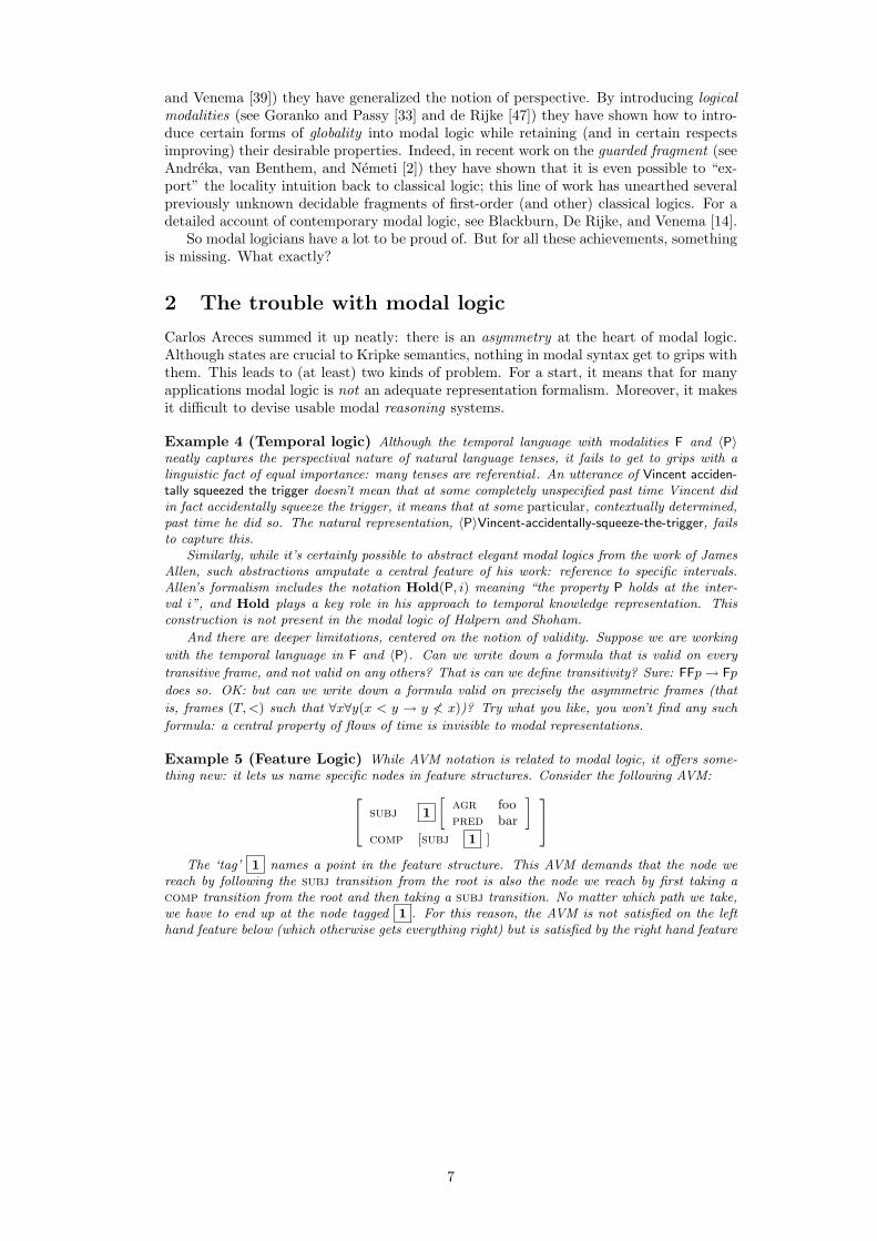
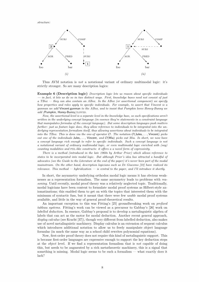
Example 5 (Feature Logic) While AVM notation is related to modal logic, it offers some-thing new: it lets us name specific nodes in feature structures. Consider the following AVM: subj 1

[agr foopred bar

]comp [subj 1 ]

The ‘tag’ 1 names a point in the feature structure. This AVM demands that the node we

reach by following the subj transition from the root is also the node we reach by first taking acomp transition from the root and then taking a subj transition. No matter which path we take,we have to end up at the node tagged 1 . For this reason, the AVM is not satisfied on the lefthand feature below (which otherwise gets everything right) but is satisfied by the right hand feature

7

structure:

1

2 1

compcomp

pred predagr agr

subj

subj

subj

subj

(ii)(i)

foo foobar bar

@@

@@@R

��

��/s s s?

s@

@@

@@R

��

��/s s �

s@

@@

@@R

��

��/s s@

@@

@@R

��

��/s s

Thus AVM notation is not a notational variant of ordinary multimodal logic: it’sstrictly stronger. So are many description logics:

Example 6 (Description logic) Description logic lets us reason about specific individuals— in fact, it lets us do so in two distinct ways. First, knowledge bases need not consist of justa TBox — they can also contain an ABox. In the ABox (or assertional component) we specifyhow properties and roles apply to specific individuals. For example, to assert that Vincent is agunman we add Vincent:gunman to the ABox, and to insist that Pumpkin loves Honey-Bunny weadd (Pumpkin, Honey-Bunny):loves.

Now, the assertional level is a separate level in the knowledge base, so such specifications aren’twritten in the underlying concept language (in essence they’re statements in a constraint languagethat manipulates formulas of the concept language). But some description languages push mattersfurther: just as feature logic does, they allow reference to individuals to be integrated into the un-derlying representation formalism itself, thus allowing assertions about individuals to be integratedinto the TBox. This is done via the one-of operator O. The notation O(Jules, . . . ,Vincent) picksout one of the individuals Jules,. . . , Vincent, and O(Mia) picks out Mia. In short, we now havea concept language rich enough to refer to specific individuals. Such a concept language is nota notational variant of ordinary multimodal logic, or even multimodal logic enriched with (say)counting modalities and pdl-like constructs: it offers a a novel form of expressivity.

There is a method (introduced in the late 1960s by Arthur Prior) which allows reference to

states to be incorporated into modal logic. But although Prior’s idea has attracted a handful of

advocates (see the Guide to the Literature at the end of the paper) it’s never been part of the modal

mainstream. On the other hand, description logicians such as De Giacomo [22] have realized its

relevance. This method — hybridization — is central to the paper, and I’ll introduce it shortly.

In short, the asymmetry underlying orthodox modal logic means it has obvious weak-nesses as a representation formalism. The same asymmetry leads to problems with rea-soning. Until recently, modal proof theory was a relatively neglected topic. Traditionally,modal logicians have been content to formulate modal proof systems as Hilbert-style ax-iomatizations; this enabled them to get on with the topics that interested them with theminimum of syntactic fuss, but it meant that there were few usable modal proof systemsavailable, and little in the way of general proof-theoretical results.

An important exception to this was Fitting’s [25] groundbreaking work on prefixedtableau systems. Fitting’s work can be viewed as a precursor to Gabbay’s [26] work onlabelled deduction. In essence, Gabbay’s proposal is to develop a metalinguistic algebra oflabels that can act as the motor for modal deduction. Another recent general approach,display calculus (see Kracht [37]), though very different from labelled deduction, also makesuse of novel metalinguistic machinery. Display calculus is an extension of sequent calculuswhich introduces additional notation to allow us to freely manipulate object languageformulas (in much the same way as a school child rewrites polynomial equations).

Now, first-order proof theory does not require this kind of metalinguistic support. Thisis because first-order languages are expressive enough to support the key deduction stepsat the object level. If we find a representation formalism that is not capable of doingthis, but needs to be augmented by a rich metatheoretic machinery, this is a signal thatsomething is missing. Modal logic seems to be such a formalism — what exactly does itlack?

8

If we look at the Fitting-Gabbay tradition, an answer practically leaps off the page:we need to be able to deal with states explicitly. We need to be able to name them, reasonabout their identity, and reason about the transitions that are possible between them.In essence, labelled deduction in its various forms supplies metalinguistic equipment forcarrying out these tasks, and this leads to modally natural proof systems. In particular,labelled deduction successfully captures the key intuition underlying Kripke semantics,that of a little automaton working it’s way through a graphlike structure — except thatthe automaton’s deductive task is to try and build such a structure, not explore a pre-existing one.

Summing up, whether we think about representation or reasoning the conclusion isthe same: modal logic’s lack of mechanisms for dealing with states explicitly is a genuineweakness.

3 Hybrid logic

Hybrid languages provide a genuinely modal solution to this problem. Modal logic maynot be perfect — but it’s certainly a most remarkable fragment of classical logic. How canwe add reference to states without destroying it?

Let’s go back to basics. Modal logic allows us to form complex formulas out of atomicformulas using booleans and modalities. There’s only formulas, nothing else. So if we wantto name states and remain modal, we should find a way of naming states using formulas.

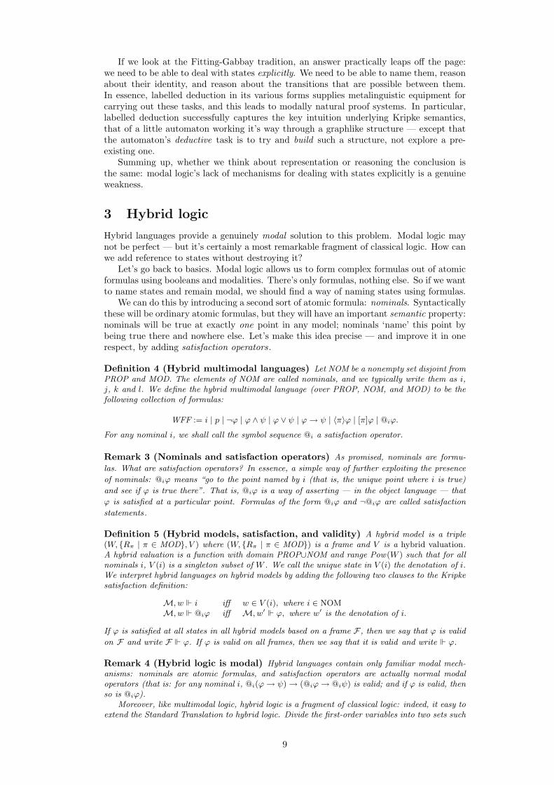
We can do this by introducing a second sort of atomic formula: nominals. Syntacticallythese will be ordinary atomic formulas, but they will have an important semantic property:nominals will be true at exactly one point in any model; nominals ‘name’ this point bybeing true there and nowhere else. Let’s make this idea precise — and improve it in onerespect, by adding satisfaction operators.

Definition 4 (Hybrid multimodal languages) Let NOM be a nonempty set disjoint fromPROP and MOD. The elements of NOM are called nominals, and we typically write them as i,j, k and l. We define the hybrid multimodal language (over PROP, NOM, and MOD) to be thefollowing collection of formulas:

WFF := i | p | ¬ϕ | ϕ ∧ ψ | ϕ ∨ ψ | ϕ→ ψ | 〈π〉ϕ | [π]ϕ | @iϕ.

For any nominal i, we shall call the symbol sequence @i a satisfaction operator.

Remark 3 (Nominals and satisfaction operators) As promised, nominals are formu-

las. What are satisfaction operators? In essence, a simple way of further exploiting the presence

of nominals: @iϕ means “go to the point named by i (that is, the unique point where i is true)

and see if ϕ is true there”. That is, @iϕ is a way of asserting — in the object language — that

ϕ is satisfied at a particular point. Formulas of the form @iϕ and ¬@iϕ are called satisfaction

statements.

Definition 5 (Hybrid models, satisfaction, and validity) A hybrid model is a triple(W, {Rπ | π ∈ MOD}, V ) where (W, {Rπ | π ∈ MOD}) is a frame and V is a hybrid valuation.A hybrid valuation is a function with domain PROP∪NOM and range Pow(W ) such that for allnominals i, V (i) is a singleton subset of W . We call the unique state in V (i) the denotation of i.We interpret hybrid languages on hybrid models by adding the following two clauses to the Kripkesatisfaction definition:

M, w i iff w ∈ V (i), where i ∈ NOMM, w @iϕ iff M, w′ ϕ, where w′ is the denotation of i.

If ϕ is satisfied at all states in all hybrid models based on a frame F , then we say that ϕ is valid

on F and write F ϕ. If ϕ is valid on all frames, then we say that it is valid and write ϕ.

Remark 4 (Hybrid logic is modal) Hybrid languages contain only familiar modal mech-anisms: nominals are atomic formulas, and satisfaction operators are actually normal modaloperators (that is: for any nominal i, @i(ϕ→ ψ)→ (@iϕ→ @iψ) is valid; and if ϕ is valid, thenso is @iϕ).

Moreover, like multimodal logic, hybrid logic is a fragment of classical logic: indeed, it easy toextend the Standard Translation to hybrid logic. Divide the first-order variables into two sets such

9

that one contains the reserved variable x and the variables used to translate familiar modalities,while the other contains a first-order variable xi for every nominal i. Define:

STx(i) = x = xi, i ∈ NOMSTx(@iϕ) = (STx(ϕ))[xi/x]

Clearly M, w ϕ iff M |= STx(ϕ)[w, V (i), . . . , V (j)], where x, xi, . . .xj are the free variablesin STx(ϕ). Nominals correspond to free variables, and (as the substitution [xi/x] makes clear)satisfaction operators let us switch our perspective from the current state to named states.

So far, so modal — but what about computational complexity? No change. As Areces, Black-

burn and Marx [4] show, hybrid logic is (up to a polynomial) no more complex than multimodal

logic: deciding the validity of hybrid formulas is a PSPACE-complete problem.

Remark 5 (Hybrid logic is hybrid) Any modal logic is a fragment of classical logic — but

hybrid logic takes matters a lot further. The near-atomic satisfaction statement @ij asserts that

the states named by i and j are identical, thus we have incorporated part of the classical theory of

equality. Similarly @i〈π〉j means that the state named by j is an Rπ-successor of the state named

by i, so we’ve incorporated the classical ability to make assertions about the relations that hold

between specific states. Thus hybrid logic is a genuine hybrid: it brings to modal logic the classical

concepts of identity and reference.

With this extra classical power at out disposal, it is straightforward to fix the repre-sentational problems noted in the previous section.

Example 7 (Temporal logic) First, although Vincent accidentally squeezed the trigger can’tbe correctly represented in the ordinary temporal language in F and 〈P〉 , it can be with the help ofnominals: 〈P〉(i∧Vincent-accidentally-squeeze-the-trigger) locates the trigger-squeezing not merelyin the past, but at a specific temporal state there, namely the one named by i.

Second, if we want to work with interval-based temporal models, we can now do so in a waythat is faithful to the work of James Allen: the satisfaction statement @iϕ is a clear analog ofAllen’s Hold(i, ϕ) construct. More on this in Section 6.

Third, we also solve the deeper issue concerning definability: i → ¬FFi defines asymmetry

(that is, it is valid on all asymmetric frames and no others). More on this in Section 5.

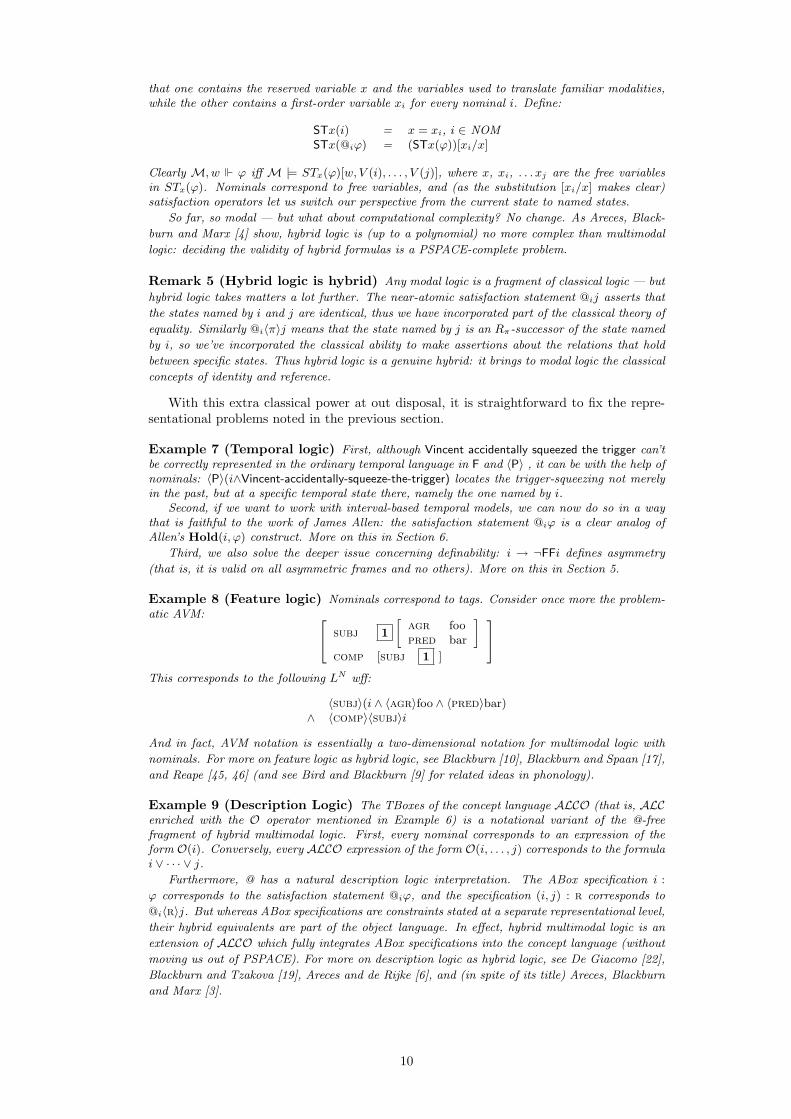
Example 8 (Feature logic) Nominals correspond to tags. Consider once more the problem-atic AVM: subj 1

[agr foopred bar

]comp [subj 1 ]

This corresponds to the following LN wff:

〈subj〉(i ∧ 〈agr〉foo ∧ 〈pred〉bar)∧ 〈comp〉〈subj〉i

And in fact, AVM notation is essentially a two-dimensional notation for multimodal logic with

nominals. For more on feature logic as hybrid logic, see Blackburn [10], Blackburn and Spaan [17],

and Reape [45, 46] (and see Bird and Blackburn [9] for related ideas in phonology).

Example 9 (Description Logic) The TBoxes of the concept language ALCO (that is, ALCenriched with the O operator mentioned in Example 6) is a notational variant of the @-freefragment of hybrid multimodal logic. First, every nominal corresponds to an expression of theform O(i). Conversely, every ALCO expression of the form O(i, . . . , j) corresponds to the formulai ∨ · · · ∨ j.

Furthermore, @ has a natural description logic interpretation. The ABox specification i :

ϕ corresponds to the satisfaction statement @iϕ, and the specification (i, j) : r corresponds to

@i〈r〉j. But whereas ABox specifications are constraints stated at a separate representational level,

their hybrid equivalents are part of the object language. In effect, hybrid multimodal logic is an

extension of ALCO which fully integrates ABox specifications into the concept language (without

moving us out of PSPACE). For more on description logic as hybrid logic, see De Giacomo [22],

Blackburn and Tzakova [19], Areces and de Rijke [6], and (in spite of its title) Areces, Blackburn

and Marx [3].

10

4 Hybrid reasoning

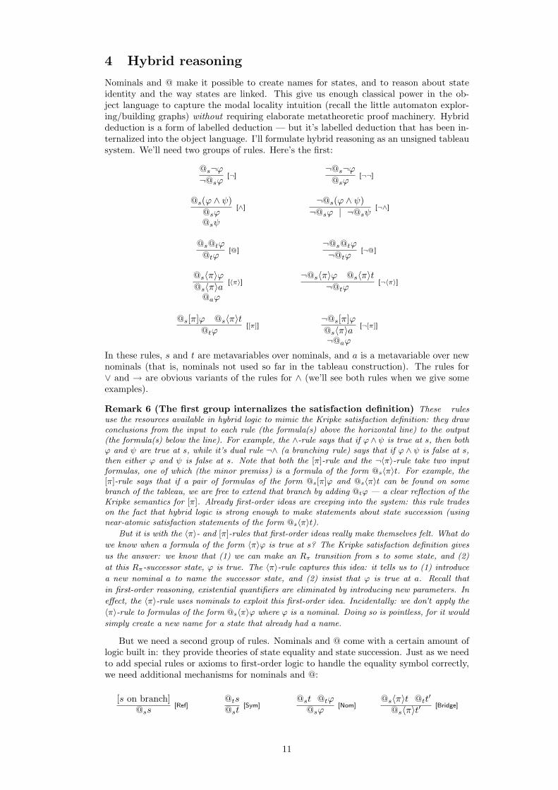
Nominals and @ make it possible to create names for states, and to reason about stateidentity and the way states are linked. This give us enough classical power in the ob-ject language to capture the modal locality intuition (recall the little automaton explor-ing/building graphs) without requiring elaborate metatheoretic proof machinery. Hybriddeduction is a form of labelled deduction — but it’s labelled deduction that has been in-ternalized into the object language. I’ll formulate hybrid reasoning as an unsigned tableausystem. We’ll need two groups of rules. Here’s the first:

@s¬ϕ¬@sϕ

[¬]¬@s¬ϕ

@sϕ[¬¬]

@s(ϕ ∧ ψ)@sϕ

[∧]¬@s(ϕ ∧ ψ)¬@sϕ | ¬@sψ

[¬∧]

@sψ

@s@tϕ

@tϕ[@]

¬@s@tϕ

¬@tϕ[¬@]

@s〈π〉ϕ@s〈π〉a

[〈π〉]¬@s〈π〉ϕ @s〈π〉t

¬@tϕ[¬〈π〉]

@aϕ

@s[π]ϕ @s〈π〉t@tϕ

[[π]]¬@s[π]ϕ@s〈π〉a

[¬[π]]

¬@aϕ

In these rules, s and t are metavariables over nominals, and a is a metavariable over newnominals (that is, nominals not used so far in the tableau construction). The rules for∨ and → are obvious variants of the rules for ∧ (we’ll see both rules when we give someexamples).

Remark 6 (The first group internalizes the satisfaction definition) These rulesuse the resources available in hybrid logic to mimic the Kripke satisfaction definition: they drawconclusions from the input to each rule (the formula(s) above the horizontal line) to the output(the formula(s) below the line). For example, the ∧-rule says that if ϕ ∧ ψ is true at s, then bothϕ and ψ are true at s, while it’s dual rule ¬∧ (a branching rule) says that if ϕ ∧ ψ is false at s,then either ϕ and ψ is false at s. Note that both the [π]-rule and the ¬〈π〉-rule take two inputformulas, one of which (the minor premiss) is a formula of the form @s〈π〉t. For example, the[π]-rule says that if a pair of formulas of the form @s[π]ϕ and @s〈π〉t can be found on somebranch of the tableau, we are free to extend that branch by adding @tϕ — a clear reflection of theKripke semantics for [π]. Already first-order ideas are creeping into the system: this rule tradeson the fact that hybrid logic is strong enough to make statements about state succession (usingnear-atomic satisfaction statements of the form @s〈π〉t).

But it is with the 〈π〉- and [π]-rules that first-order ideas really make themselves felt. What do

we know when a formula of the form 〈π〉ϕ is true at s? The Kripke satisfaction definition gives

us the answer: we know that (1) we can make an Rπ transition from s to some state, and (2)

at this Rπ-successor state, ϕ is true. The 〈π〉-rule captures this idea: it tells us to (1) introduce

a new nominal a to name the successor state, and (2) insist that ϕ is true at a. Recall that

in first-order reasoning, existential quantifiers are eliminated by introducing new parameters. In

effect, the 〈π〉-rule uses nominals to exploit this first-order idea. Incidentally: we don’t apply the

〈π〉-rule to formulas of the form @s〈π〉ϕ where ϕ is a nominal. Doing so is pointless, for it would

simply create a new name for a state that already had a name.

But we need a second group of rules. Nominals and @ come with a certain amount oflogic built in: they provide theories of state equality and state succession. Just as we needto add special rules or axioms to first-order logic to handle the equality symbol correctly,we need additional mechanisms for nominals and @:

[s on branch]@ss

[Ref]@ts@st

[Sym]@st @tϕ

@sϕ[Nom]

@s〈π〉t @tt′

@s〈π〉t′[Bridge]

11

Remark 7 (The second group is a essentially a classical rewrite system) The

Ref rule says that if a nominal s occurs in any formula on a branch, then we are free to add

@ss to that branch; this is clearly an analog of the first-order reflexivity rule for =, just as the

Sym rule is an analog of the first-order symmetry rule for =. What about transitivity? From @st

and @tt′ we should be able to conclude @st

′. But this is a special case of Nom, namely when ϕ

is chosen to be a nominal t′. More generally, Nom ensures that identical states carry identical

information, while Bridge ensures that states are coherently linked. In first-order terms, these

rules ensure that state identity is not merely an equivalence relation but a congruence.

As with any tableau system, we prove formulas by systematically trying to falsifythem. Suppose we want to prove ϕ. We choose a nominal (say i) that does not occurin ϕ (this acts as a name for the falsifying state that is supposed to exist), prefix ϕ with¬@i, and start applying rules. If the tableau closes (that is, if every branch containssome formula and its negation), then ϕ is proved. On the other hand, suppose we reacha stage where we have applied the appropriate connective rule to every complex formula(or in the case of [π]-formulas, we have applied the [π]-rule to every pair of formulas ofthe form @s[π]ϕ, @s〈π〉t on the same branch; and analogously for ¬〈π〉-formulas) and noapplication of the rewrite rules yields anything new. If the tableau we have constructedcontains open branches (that is, branches not containing conflicting formulas), then ϕ isnot valid (and hence not provable), and the near-atomic satisfaction statements on theopen branch specify a countermodel.

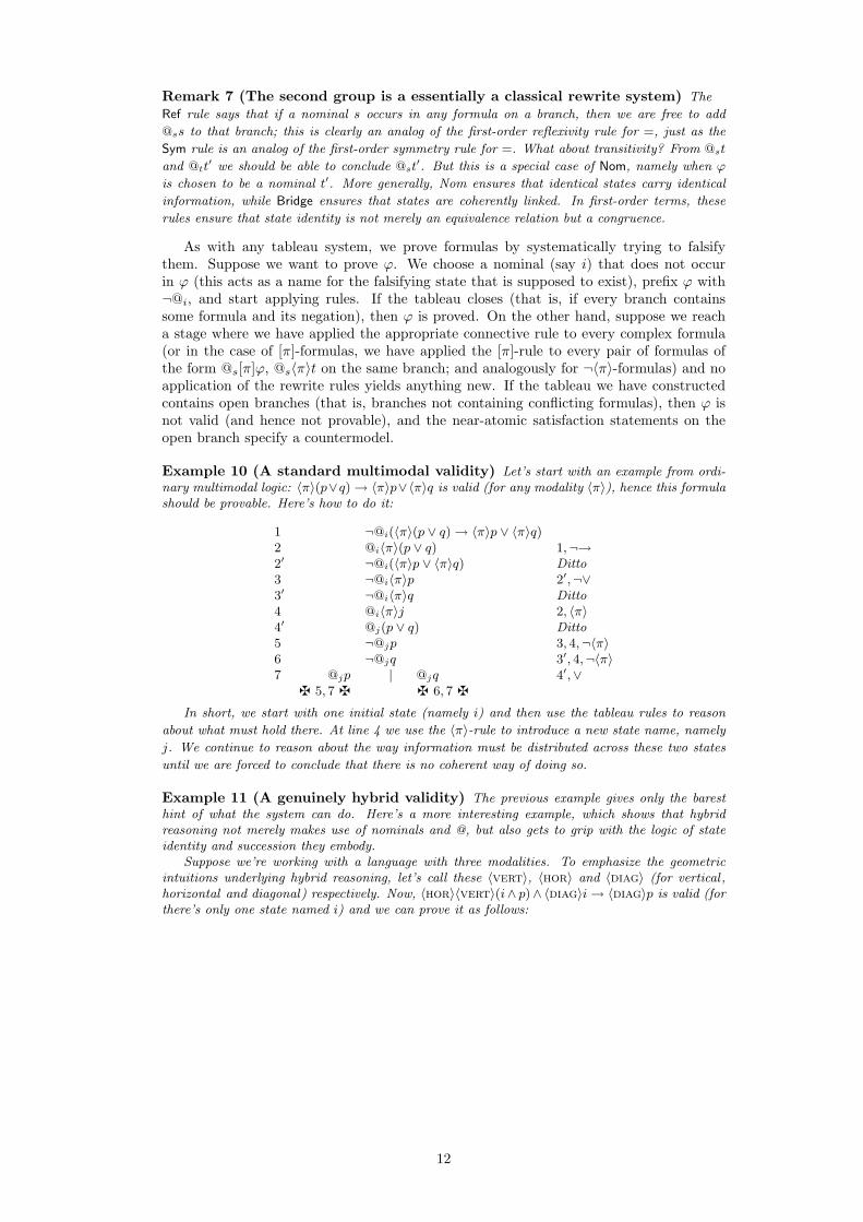
Example 10 (A standard multimodal validity) Let’s start with an example from ordi-nary multimodal logic: 〈π〉(p∨q)→ 〈π〉p∨〈π〉q is valid (for any modality 〈π〉), hence this formulashould be provable. Here’s how to do it:

1 ¬@i(〈π〉(p ∨ q)→ 〈π〉p ∨ 〈π〉q)2 @i〈π〉(p ∨ q) 1,¬→2′ ¬@i(〈π〉p ∨ 〈π〉q) Ditto3 ¬@i〈π〉p 2′,¬∨3′ ¬@i〈π〉q Ditto4 @i〈π〉j 2, 〈π〉4′ @j(p ∨ q) Ditto5 ¬@jp 3, 4,¬〈π〉6 ¬@jq 3′, 4,¬〈π〉7 @jp | @jq 4′,∨

z 5, 7 z z 6, 7 z

In short, we start with one initial state (namely i) and then use the tableau rules to reason

about what must hold there. At line 4 we use the 〈π〉-rule to introduce a new state name, namely

j. We continue to reason about the way information must be distributed across these two states

until we are forced to conclude that there is no coherent way of doing so.

Example 11 (A genuinely hybrid validity) The previous example gives only the baresthint of what the system can do. Here’s a more interesting example, which shows that hybridreasoning not merely makes use of nominals and @, but also gets to grip with the logic of stateidentity and succession they embody.

Suppose we’re working with a language with three modalities. To emphasize the geometricintuitions underlying hybrid reasoning, let’s call these 〈vert〉, 〈hor〉 and 〈diag〉 (for vertical ,horizontal and diagonal) respectively. Now, 〈hor〉〈vert〉(i∧ p)∧ 〈diag〉i→ 〈diag〉p is valid (forthere’s only one state named i) and we can prove it as follows:

12

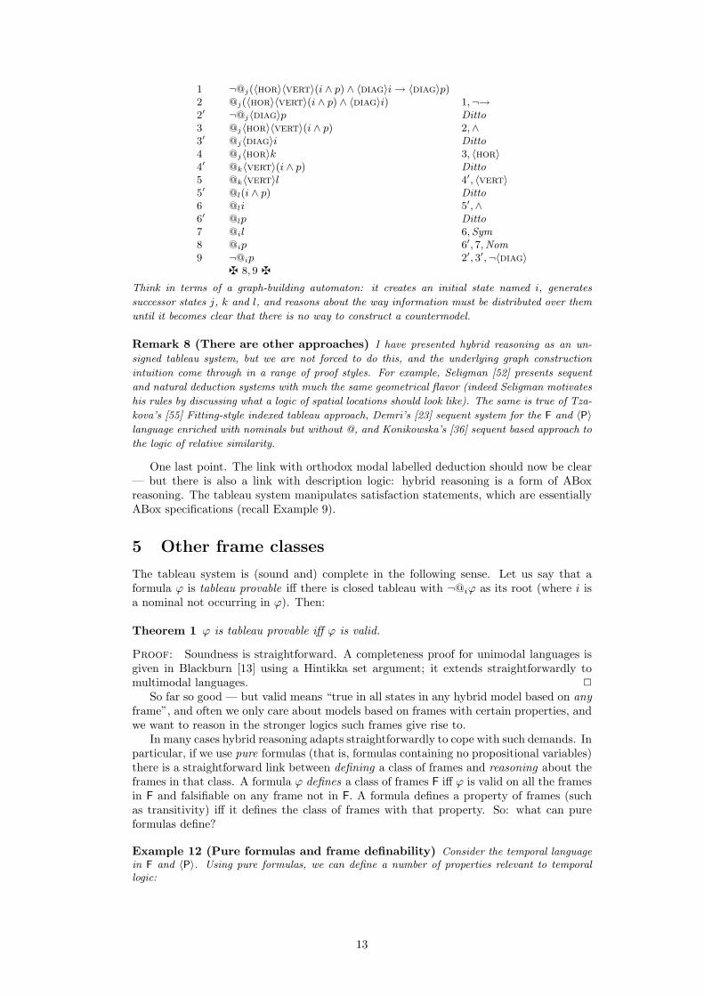
1 ¬@j(〈hor〉〈vert〉(i ∧ p) ∧ 〈diag〉i→ 〈diag〉p)2 @j(〈hor〉〈vert〉(i ∧ p) ∧ 〈diag〉i) 1,¬→2′ ¬@j〈diag〉p Ditto3 @j〈hor〉〈vert〉(i ∧ p) 2,∧3′ @j〈diag〉i Ditto4 @j〈hor〉k 3, 〈hor〉4′ @k〈vert〉(i ∧ p) Ditto5 @k〈vert〉l 4′, 〈vert〉5′ @l(i ∧ p) Ditto6 @li 5′,∧6′ @lp Ditto7 @il 6,Sym8 @ip 6′, 7,Nom9 ¬@ip 2′, 3′,¬〈diag〉

z 8, 9 z

Think in terms of a graph-building automaton: it creates an initial state named i, generates

successor states j, k and l, and reasons about the way information must be distributed over them

until it becomes clear that there is no way to construct a countermodel.

Remark 8 (There are other approaches) I have presented hybrid reasoning as an un-

signed tableau system, but we are not forced to do this, and the underlying graph construction

intuition come through in a range of proof styles. For example, Seligman [52] presents sequent

and natural deduction systems with much the same geometrical flavor (indeed Seligman motivates

his rules by discussing what a logic of spatial locations should look like). The same is true of Tza-

kova’s [55] Fitting-style indexed tableau approach, Demri’s [23] sequent system for the F and 〈P〉language enriched with nominals but without @, and Konikowska’s [36] sequent based approach to

the logic of relative similarity.

One last point. The link with orthodox modal labelled deduction should now be clear— but there is also a link with description logic: hybrid reasoning is a form of ABoxreasoning. The tableau system manipulates satisfaction statements, which are essentiallyABox specifications (recall Example 9).

5 Other frame classes

The tableau system is (sound and) complete in the following sense. Let us say that aformula ϕ is tableau provable iff there is closed tableau with ¬@iϕ as its root (where i isa nominal not occurring in ϕ). Then:

Theorem 1 ϕ is tableau provable iff ϕ is valid.

Proof: Soundness is straightforward. A completeness proof for unimodal languages isgiven in Blackburn [13] using a Hintikka set argument; it extends straightforwardly tomultimodal languages. 2

So far so good — but valid means “true in all states in any hybrid model based on anyframe”, and often we only care about models based on frames with certain properties, andwe want to reason in the stronger logics such frames give rise to.

In many cases hybrid reasoning adapts straightforwardly to cope with such demands. Inparticular, if we use pure formulas (that is, formulas containing no propositional variables)there is a straightforward link between defining a class of frames and reasoning about theframes in that class. A formula ϕ defines a class of frames F iff ϕ is valid on all the framesin F and falsifiable on any frame not in F. A formula defines a property of frames (suchas transitivity) iff it defines the class of frames with that property. So: what can pureformulas define?

Example 12 (Pure formulas and frame definability) Consider the temporal languagein F and 〈P〉. Using pure formulas, we can define a number of properties relevant to temporallogic:

13

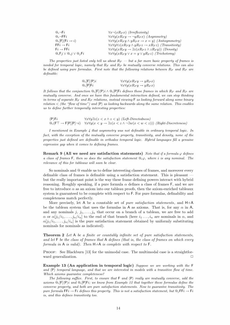
@i¬Fi ∀x¬(xRFx) (Irreflexivity)@i¬FFi ∀x∀y(xRF y → ¬yRFx) (Asymmetry)@i[F](Fi→ i) ∀x∀y(xRF y ∧ yRFx→ x = y) (Antisymmetry)FFi→ Fi ∀x∀y∀z(xRF y ∧ yRF z → xRF z) (Transitivity)Fi→ FFi ∀x∀y(xRF y → ∃z(xRF z ∧ zRF y)) (Density)@iFj ∨@ij ∨@jFi ∀x∀y(xRF y ∨ x = y ∨ yRF z) (Trichotomy)

The properties just listed only tell us about RF — but a far more basic property of frames isneeded for temporal logic, namely that RF and RP be mutually converse relations. This can alsobe defined using pure formulas. First note that the following relations between RF and RP aredefinable:

@i[F]〈P〉i ∀x∀y(xRF y → yRPx)@i[P]Fi ∀x∀y(xRP y → yRFx)

It follows that the conjunction @i[F]〈P〉i ∧@i[P]Fi defines those frames in which RF and RP aremutually converse. And once we have this fundamental interaction defined, we can stop thinkingin terms of separate RF and RP relations, instead viewing F as looking forward along some binaryrelation < (the “flow of time”) and 〈P〉 as looking backwards along the same relation. This enablesus to define further temporally interesting properties:

〈P〉Fi ∀x∀y∃z(z < x ∧ z < y) (Left-Directedness)@i(F> → F[P][P]¬i) ∀x∀y(x < y → ∃z(x < z ∧ ¬∃w(x < w < z))) (Right-Discreteness)

I mentioned in Example 4 that asymmetry was not definable in ordinary temporal logic. In

fact, with the exception of the mutually converse property, transitivity, and density, none of the

properties just defined are definable in orthodox temporal logic. Hybrid languages fill a genuine

expressive gap when it comes to defining frames.

Remark 9 (All we need are satisfaction statements) Note that if a formula ϕ defines

a class of frames F, then so does the satisfaction statement @iϕ, where i is any nominal. The

relevance of this for tableaux will soon be clear.

So nominals and @ enable us to define interesting classes of frames, and moreover everydefinable class of frames is definable using a satisfaction statement. This is pleasant —but the really important point is the way these frame defining powers interact with hybridreasoning. Roughly speaking, if a pure formula α defines a class of frames F, and we arefree to introduce α as an axiom into our tableau proofs, then the axiom-enriched tableauxsystem is guaranteed to be complete with respect to F. For pure formulas, definability andcompleteness match perfectly.

More precisely, let A be a countable set of pure satisfaction statements, and H+Abe the tableau system that uses the formulas in A as axioms. That is, for any α in A,and any nominals j, j1, . . . , jn that occur on a branch of a tableau, we are free to addα or α[j1/i1, . . . , jn/in] to the end of that branch (here i1 . . . , in are nominals in α, andα[j1/i1, . . . , jn/in] is the pure satisfaction statement obtained by uniformly substitutingnominals for nominals as indicated).

Theorem 2 Let A be a finite or countably infinite set of pure satisfaction statements,and let F be the class of frames that A defines (that is, the class of frames on which everyformula in A is valid). Then H+A is complete with respect to F.

Proof: See Blackburn [13] for the unimodal case. The multimodal case is a straightfor-ward generalization. 2

Example 13 (An application in temporal logic) Suppose we are working with the Fand 〈P〉 temporal language, and that we are interested in models with a transitive flow of time.Which axioms guarantee completeness?

The following suffice. First, to ensure that F and 〈P〉 really are mutually converse, add theaxioms @i[F]〈P〉i and @i[P]Fi; we know from Example 12 that together these formulas define theconverse property, and both are pure satisfaction statements. Now to guarantee transitivity. Thepure formula FFi→ Fi defines this property. This is not a satisfaction statement, but @jFFi→ Fiis, and this defines transitivity too.

14

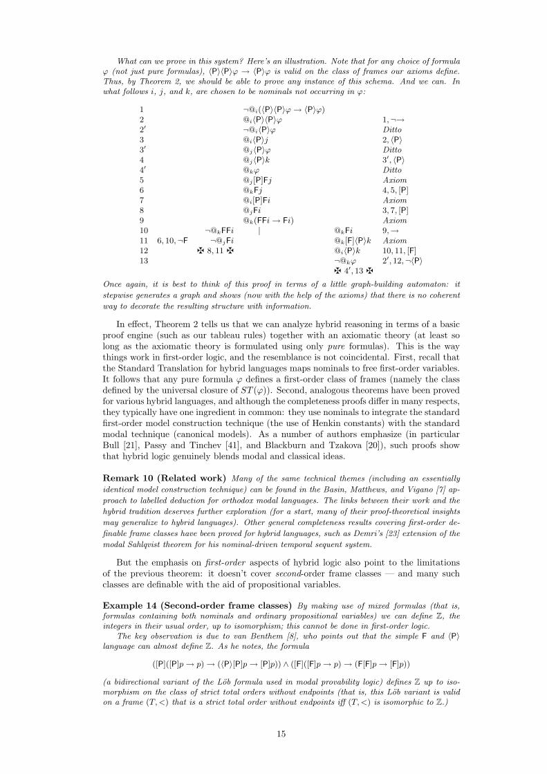
What can we prove in this system? Here’s an illustration. Note that for any choice of formulaϕ (not just pure formulas), 〈P〉〈P〉ϕ → 〈P〉ϕ is valid on the class of frames our axioms define.Thus, by Theorem 2, we should be able to prove any instance of this schema. And we can. Inwhat follows i, j, and k, are chosen to be nominals not occurring in ϕ:

1 ¬@i(〈P〉〈P〉ϕ→ 〈P〉ϕ)2 @i〈P〉〈P〉ϕ 1,¬→2′ ¬@i〈P〉ϕ Ditto3 @i〈P〉j 2, 〈P〉3′ @j〈P〉ϕ Ditto4 @j〈P〉k 3′, 〈P〉4′ @kϕ Ditto5 @j [P]Fj Axiom6 @kFj 4, 5, [P]7 @i[P]Fi Axiom8 @jFi 3, 7, [P]9 @k(FFi→ Fi) Axiom10 ¬@kFFi | @kFi 9,→11 6, 10,¬F ¬@jFi @k[F]〈P〉k Axiom12 z 8, 11 z @i〈P〉k 10, 11, [F]13 ¬@kϕ 2′, 12,¬〈P〉

z 4′, 13 z

Once again, it is best to think of this proof in terms of a little graph-building automaton: it

stepwise generates a graph and shows (now with the help of the axioms) that there is no coherent

way to decorate the resulting structure with information.

In effect, Theorem 2 tells us that we can analyze hybrid reasoning in terms of a basicproof engine (such as our tableau rules) together with an axiomatic theory (at least solong as the axiomatic theory is formulated using only pure formulas). This is the waythings work in first-order logic, and the resemblance is not coincidental. First, recall thatthe Standard Translation for hybrid languages maps nominals to free first-order variables.It follows that any pure formula ϕ defines a first-order class of frames (namely the classdefined by the universal closure of ST (ϕ)). Second, analogous theorems have been provedfor various hybrid languages, and although the completeness proofs differ in many respects,they typically have one ingredient in common: they use nominals to integrate the standardfirst-order model construction technique (the use of Henkin constants) with the standardmodal technique (canonical models). As a number of authors emphasize (in particularBull [21], Passy and Tinchev [41], and Blackburn and Tzakova [20]), such proofs showthat hybrid logic genuinely blends modal and classical ideas.

Remark 10 (Related work) Many of the same technical themes (including an essentially

identical model construction technique) can be found in the Basin, Matthews, and Vigano [7] ap-

proach to labelled deduction for orthodox modal languages. The links between their work and the

hybrid tradition deserves further exploration (for a start, many of their proof-theoretical insights

may generalize to hybrid languages). Other general completeness results covering first-order de-

finable frame classes have been proved for hybrid languages, such as Demri’s [23] extension of the

modal Sahlqvist theorem for his nominal-driven temporal sequent system.

But the emphasis on first-order aspects of hybrid logic also point to the limitationsof the previous theorem: it doesn’t cover second-order frame classes — and many suchclasses are definable with the aid of propositional variables.

Example 14 (Second-order frame classes) By making use of mixed formulas (that is,formulas containing both nominals and ordinary propositional variables) we can define Z, theintegers in their usual order, up to isomorphism; this cannot be done in first-order logic.

The key observation is due to van Benthem [8], who points out that the simple F and 〈P〉language can almost define Z. As he notes, the formula

([P]([P]p→ p)→ (〈P〉[P]p→ [P]p)) ∧ ([F]([F]p→ p)→ (F[F]p→ [F]p))

(a bidirectional variant of the Lob formula used in modal provability logic) defines Z up to iso-morphism on the class of strict total orders without endpoints (that is, this Lob variant is validon a frame (T,<) that is a strict total order without endpoints iff (T,<) is isomorphic to Z.)

15

But it follows from standard modal results that we can’t define strict total order without end-

points using only propositional variables — and this is where nominals come to the rescue. We

have already seen that there are (pure) formulas defining the mutual converse property of F and

〈P〉, transitivity, irreflexivity and trichotomy. Furthermore, the formulas F> and 〈P〉> ensure

that there are no endpoints. So the conjunction of all these (pure) formulas defines the class of

strict total orders without endpoints — and hence conjoining the Lob variant yields a (mixed)

formula valid on precisely the frames isomorphic to Z. In a similar way, using a mixed formula

it is possible to define N, the natural in their usual order up to isomorphism; see Blackburn [11]

for details. The second-order aspects of hybrid languages deserve further study.

The result has another limitation: it gives no computational information. While thebasic satisfaction problem for hybrid languages is PSPACE-complete, adding further ax-ioms can have a wide range of effects: they may lower the problem into NP, leave it inPSPACE or lift it to EXPTIME (see Areces, Blackburn and Marx [3] for examples of allthree possibilities). Nor is it difficult to devise axioms which result in logics with unde-cidable satisfaction problems. So the previous result tells us nothing about proof searchor termination: it simply draws attention to a group of logic which are well-behaved fromthe perspective of completeness theory. It may well be that proof-theoretical and com-putational insights from the labelled deduction and description logic communities have arole to play in analyzing these logics further.

6 Binding nominals to states

From the perspective of the Standard Translation, adding nominals to a modal languageis in effect to add free variables over states. This immediately suggest a further extension:why not bind these “free variables”, thus giving ourselves access to even more expressivepower? I’ll give a brief sketch of such logics, and then turn to the issue that interests mehere: why they are relevant to knowledge representation.

Example 15 (Losers, jerks, and politicians) Let’s jump into the realms of pop-psychology and define a loser to be someone with no self-respect. Now, we can’t define this conceptin the hybrid logics we have seen so far; the closest we get is:

i ∧ ¬〈respect〉i.

This says that a specific individual i lacks self-respect. But we want more: we want a formulathat is true at precisely those nodes (individuals) which lack a reflexive respect arc. We can getwhat we want by binding i out:

∃x(x ∧ ¬〈respect〉x).This sentence is true at precisely those those nodes at which it is possible to bind x to the currentstate, but impossible to loop back to the current state via the respect relation.

Two remarks. First, the idea of binding nominals to the current state is so important in hybridlogic that a special notation (namely ↓) has been introduced for it. So the previous sentence wouldnormally be written:

↓x.¬〈respect〉x.Second, as these examples illustrate, orthodox variable notation (x, y, z, and so on) is usuallyused for bound nominals.

OK — let’s now define a jerk to be an idiot who admires himself:

idiot ∧ ↓x.〈admires〉x.

This sentence is satisfied at precisely those nodes which (1) have the idiot property, and (2) fromwhich it is possible to take a reflexive step via the admires relation.

Finally, let’s define a politician as a smooth talker such that everyone he talks to mistrustshim:

↓x.(smooth-talker ∧ ∀y(〈talks-to〉y → ¬@y〈trusts〉x).

Note the way the @y switches the perspective from the node x (the politician) to his audience.

I won’t give a precise definition of the syntax and semantics of hybrid languages with∀ and ∃ here (you can find all this in Blackburn and Seligman [15, 16] or Blackburn andTzakova [18, 19]). The previous examples tell you pretty much everything you need toknow, and the discussion that follows should clarify things further.

16

Remark 11 (We now have first-order expressivity) Our new hybrid logic is strongenough to express any first-order concept. Here’s the Hybrid Translation from first-order rep-resentations to our new hybrid logic:

HT (xRπy) = @x〈π〉yHT (Px) = @xpHT (x = y) = @xyHT (¬ϕ) = ¬HT (ϕ)HT (ϕ ∧ ψ) = HT (ϕ) ∧HT (ψ)HT (∃vϕ) = ∃vHT (ϕ)HT (∀vϕ) = ∀vHT (ϕ).

But although we can jump straight up to full first-order power, we don’t have to. Fora start, the use of @ in the hybrid translation is crucial . If we work with the @-free sub-language, binding nominals to states with ∃ and ∀ does not yield full first-order expressivepower; for a counterexample, see Proposition 4.5 of Blackburn and Seligman [15]. Hybridlogic decomposes the action of the classical quantifiers into two subtasks: perspective-shifting (performed by @) and binding (performed by the hybrid binders ∃ and ∀).

Moreover, we’ve seen that there is a useful restricted form of these binders, namely ↓.Some recent papers have explored hybrid logics with a primitive ↓ binder (without ∃ or ∀),and it turns out that such logics characterize the notion of locality; see Areces, Blackburn,and Marx [4].

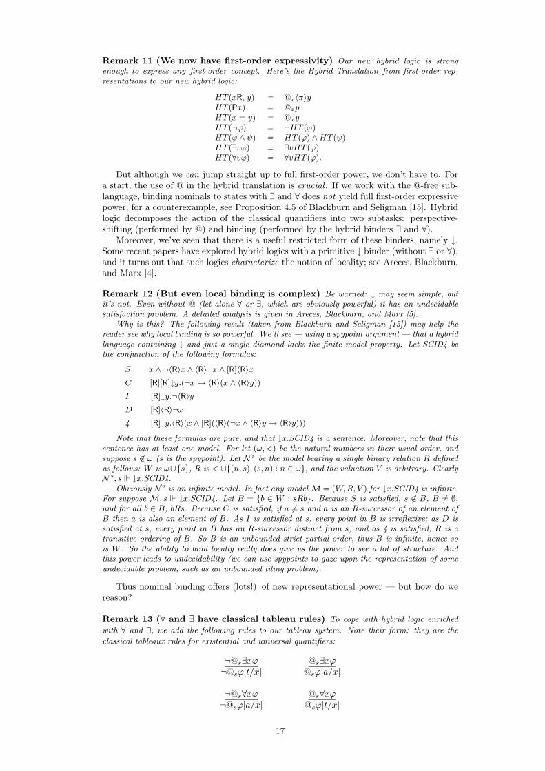
Remark 12 (But even local binding is complex) Be warned: ↓ may seem simple, butit’s not. Even without @ (let alone ∀ or ∃, which are obviously powerful) it has an undecidablesatisfaction problem. A detailed analysis is given in Areces, Blackburn, and Marx [5].

Why is this? The following result (taken from Blackburn and Seligman [15]) may help thereader see why local binding is so powerful. We’ll see — using a spypoint argument — that a hybridlanguage containing ↓ and just a single diamond lacks the finite model property. Let SCID4 bethe conjunction of the following formulas:

S x ∧ ¬〈R〉x ∧ 〈R〉¬x ∧ [R]〈R〉xC [R][R]↓y.(¬x→ 〈R〉(x ∧ 〈R〉y))I [R]↓y.¬〈R〉yD [R]〈R〉¬x4 [R]↓y.〈R〉(x ∧ [R](〈R〉(¬x ∧ 〈R〉y → 〈R〉y)))

Note that these formulas are pure, and that ↓x.SCID4 is a sentence. Moreover, note that thissentence has at least one model. For let (ω,<) be the natural numbers in their usual order, andsuppose s 6∈ ω (s is the spypoint). Let N s be the model bearing a single binary relation R definedas follows: W is ω∪{s}, R is < ∪{(n, s), (s, n) : n ∈ ω}, and the valuation V is arbitrary. ClearlyN s, s ↓x.SCID4.

Obviously N s is an infinite model. In fact any modelM = (W,R, V ) for ↓x.SCID4 is infinite.For suppose M, s ↓x.SCID4. Let B = {b ∈ W : sRb}. Because S is satisfied, s 6∈ B, B 6= ∅,and for all b ∈ B, bRs. Because C is satisfied, if a 6= s and a is an R-successor of an element ofB then a is also an element of B. As I is satisfied at s, every point in B is irreflexive; as D issatisfied at s, every point in B has an R-successor distinct from s; and as 4 is satisfied, R is atransitive ordering of B. So B is an unbounded strict partial order, thus B is infinite, hence sois W . So the ability to bind locally really does give us the power to see a lot of structure. Andthis power leads to undecidability (we can use spypoints to gaze upon the representation of someundecidable problem, such as an unbounded tiling problem).

Thus nominal binding offers (lots!) of new representational power — but how do wereason?

Remark 13 (∀ and ∃ have classical tableau rules) To cope with hybrid logic enriched

with ∀ and ∃, we add the following rules to our tableau system. Note their form: they are the

classical tableaux rules for existential and universal quantifiers:

¬@s∃xϕ @s∃xϕ¬@sϕ[t/x] @sϕ[a/x]

¬@s∀xϕ @s∀xϕ¬@sϕ[a/x] @sϕ[t/x]

17

(Important: recall that a stands for a new nominal.) But while the rules are essentially classical,don’t forget that the underlying language is different (after all, ∀ and ∃ bind formulas!). Soas well as being able to prove all the standard classical quantificational principles (for example,∀x(ϕ→ ψ)→ (ϕ→ ∀xψ), where x does not occur free in ϕ) we can also prove intrinsically modalprinciples. For example, ∃xx is valid (this says: it is always possible to bind a variable to thecurrent state). We can prove it as follows:

1 ¬@i∃xx2 ¬@ii 1,¬∃3 @ii Ref

z 2, 3 z

These rules give us a complete deduction system for hybrid logic with ∀ and ∃. Moreover, The-

orem 2 extends to these systems: adding pure axioms yields a system complete with respect to

the class of frames the axioms define. As before, “pure” simply means “contains no propositional

variables”, so we are free to make use of ∀ and ∃ in our axioms. It follows (with the help of

the Hybrid Translation) that we have a general completeness result that covers any first-order

definable class of frames. Rules for ↓ can be found in Blackburn [13].

It’s time to turn to the link with knowledge representation. I’ll approach this topic viaJames Allen’s classic work on temporal representation.

Example 16 (Allen style representations) The core of Allen’s system is an orthodoxfirst-order theory of interval structure to which the metapredicate Hold has been added: Hold(P, i)asserts that property P holds at the interval i.

Allen then goes on to elaborate his account of properties. He introduces function symbolssuggestively named and, or, not, exists, and all, for combining property symbols, together withaxioms governing them: for example

Hold(and(P,Q), i)↔ Hold(P, i) ∧ Hold(Q, i).

It’s clear Allen wants an ‘internal’ logic of terms that mirrors the ‘external’ logic of formulas. Toput it another way, although he represents properties using terms, he wants them to behave likeformulas.

This aspect of Allen’s system has been criticized (some of the axioms governing the logicalfunctions are rather odd; furthermore, as the structure of property terms is never fully specified,it’s rather unclear what can and cannot be done with them; see Turner [54] and Shoham [53]).But I’m not so much interested in the details as the general strategy — for this is now standardin AI.

For example, if you look at Russell and Norvig [48] (in particular, the discussion of ontological

engineering in Chapter 8) you’ll see that Allen’s approach has been generalized into a multistep

methodology: (1) start with a first-order language; (2) reify the language heavily (that is, treat

categories as individuals); (3) add metapredicates; and (4) when handling temporal aspects of

ontology, induce boolean structure on the terms by adding and axiomatizing the logical functions

and, or, and not (exists and all are not discussed).

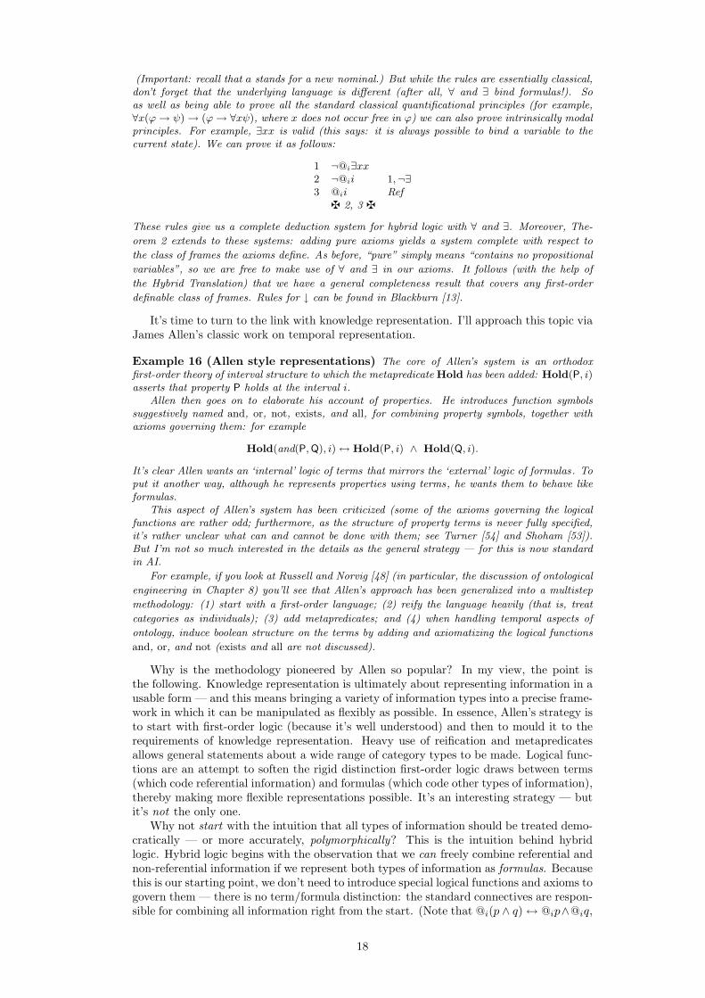
Why is the methodology pioneered by Allen so popular? In my view, the point isthe following. Knowledge representation is ultimately about representing information in ausable form — and this means bringing a variety of information types into a precise frame-work in which it can be manipulated as flexibly as possible. In essence, Allen’s strategy isto start with first-order logic (because it’s well understood) and then to mould it to therequirements of knowledge representation. Heavy use of reification and metapredicatesallows general statements about a wide range of category types to be made. Logical func-tions are an attempt to soften the rigid distinction first-order logic draws between terms(which code referential information) and formulas (which code other types of information),thereby making more flexible representations possible. It’s an interesting strategy — butit’s not the only one.

Why not start with the intuition that all types of information should be treated demo-cratically — or more accurately, polymorphically? This is the intuition behind hybridlogic. Hybrid logic begins with the observation that we can freely combine referential andnon-referential information if we represent both types of information as formulas. Becausethis is our starting point, we don’t need to introduce special logical functions and axioms togovern them — there is no term/formula distinction: the standard connectives are respon-sible for combining all information right from the start. (Note that @i(p ∧ q)↔ @ip∧@iq,

18

the hybrid analog of Allen’s axiom for the and function, isn’t something extra that needsto be stipulated: it’s just a validity of hybrid logic, and can easily be proved in the basictableau system.) Nor is there any mystery about what “property terms” are: Allen seemsto have wanted properties to have a formula-like structure, and of course, that’s exactlythe form all representations take in hybrid logic. And binding nominals with ∀ and ∃(which seems to correspond to Allen’s intentions regarding the logical functions exists andall) will take us all the way up to first-order expressivity (if that’s where we want to go).

7 The sorting strategy

In horticulture, hybrids are crossbreeds between distinct but related strains: ideally theycombine the desirable properties of the parent strains in interesting new ways. Hybridlogic is certainly hybrid in this sense. Enriching modal logic with nominals and @ leadsto systems that draw on both modal and first-order logic: we retain the locality anddecidability of modal logic, gain the ability to name states and reason about their identityand their interrelationships, and (via nominal binding) open a novel route to first-orderexpressivity.

But hybrid logic is also a sociological hybrid: it’s a meeting place for ideas from manytraditions. We’ve seen that feature logic, description logic, and labelled deduction haveindependently developed key ideas of hybrid logic, and I’ve argued that the Allen-styleontological engineering languages can be viewed as strong hybrid languages. In short, anumber of research communities, faced with similar problems (how best to represent andreason about graphlike structures) have come up with similar answers independently. Notonly do they draw (consciously or unconsciously) on modal logic, they even moved beyondthe barriers of modal orthodoxy in much the same way — the way encapsulated in hybridlogic.

But there is a third sense in which hybrid languages are hybrid, and this is perhaps themost important of all: hybrid languages are intrinsically hybrid. They allow us combinedifferent sorts of information in a single formalism. In a nutshell, hybrid logics are sortedmodal logics.

The importance of sorting has long been recognized in AI, linguistics, and philosophy:knowing that a piece of information is of a particular kind may allow us to draw usefulconclusions swiftly and easily. But sorting has been neglected in the logical tradition: manyuseful kinds of sortal reasoning (for example, chaining through an inheritance hierarchy)are regarded as too simple to be of logical interest, and every logician knows that sortedfirst-order languages offer no new expressive power.

But sorted modal languages certainly do. As we have seen, by adding a second sortof atomic formula (nominals) and a new construct to exploit it (satisfaction operators),we can describe models in more detail and define new classes of frames. Moreover, wecan create a basic reasoning system that is modally natural and supports a wide range ofricher logics. But the hybrid languages of this paper have been simple two-sorted systems.Why stop there?

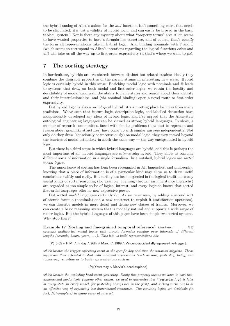
Example 17 (Sorting and fine-grained temporal reference) Blackburn [12]presents multisorted modal logics with atomic formulas ranging over intervals of differentlengths (seconds, hours, years, . . . ). This lets us build representations like

〈P〉(3.05 ∧ P.M. ∧ Friday ∧ 26th ∧March ∧ 1999 ∧ Vincent-accidentally-squeeze-the-trigger),

which locates the trigger-squeezing event at the specific day and time the notation suggests. Theselogics are then extended to deal with indexical expressions (such as now, yesterday, today, andtomorrow), enabling us to build representations such as

〈P〉(Yesterday ∧Marvin’s-head-explode),

which locates the exploding-head event yesterday. Doing this properly means we have to sort two-

dimensional modal logic (among other things, we need to guarantee that F(yesterday ∧ ϕ) is false

at every state in every model, for yesterday always lies in the past), and sorting turns out to be

an effective way of exploiting two-dimensional semantics. The resulting logics are decidable (in

fact, NP-complete) in many cases of interest.

19

Example 18 (Sorting and paths) When reasoning about branching time we often want toassert that that some event will take place in all possible paths into the future. This cannot bedone in the temporal language in F and 〈P〉, even with the help of nominals and @.

Bull [21] solved this problem by further sorting. He introduced a three-sorted modal language:in addition to propositional variables and nominals, his language contained path nominals, atomicformulas true at precisely the points on some path through a frame. He allowed explicit quantifica-tion over path nominals, and hence could define a “true at some state in every future” modality:

〈every-fut〉ϕ := ∀ρ(ρ→ F∃x(x ∧ ρ ∧ ϕ)).

Here ρ is a bound path nominal, and x a bound nominal, so this says that on every path ρ

through the current state, there is some future state x at which ϕ is true. See Goranko [32] and

Blackburn and Tzakova [20] for more on hybrid languages for paths.

I believe such examples point the way to an interesting line of work: dealing with allontological distinctions in multisorted modal languages. At present little is known aboutwhat can and cannot be done in such systems, but interesting questions abound. I hopesome equally interesting answers will soon be forthcoming.

A brief guide to the literature

I have said little about the history of hybrid logic; these notes are an attempt to put this right,and provide a route into the hybrid literature. I’ll omit references to applications of hybrid logic(such as feature logic) as these were given in the main text.

Hybrid logic was invented by Arthur Prior, the inventor of F and 〈P〉 based temporal logic(that is, tense logic). The germs of the idea seem to have emerged in discussion with C.A.Meredith in the 1950s, but the first detailed account is in Chapter V and Appendix B3 of Prior’s1967 book Past, Present, and Future [42]. Several of the papers collected in Paper on Timeand Tense [43] allude to or discuss hybrid languages, and the posthumously published bookWorlds, Times and Selves [44] is solely devoted to the topic (unfortunately, the book is only anapproximation to Prior’s intentions: it’s essentially a reconstruction, by Kit Fine, of notes foundafter Prior’s death in 1969). Prior called nominals world propositions, typically worked with veryrich hybrid languages (he bound nominals using ∀ and ∃) and made heavy use of near-atomicsatisfaction statements like the ones used in our tableau systems.

The next big step was Robert Bull’s 1970 paper “An Approach to Tense Logic” [21]. Bull in-troduced a three-sorted hybrid language (propositional variables, nominals, and path nominals),noted that the presence of ∀ and ∃ made it easy to combine the modal canonical model construc-tion with the first-order Henkin construction (and thus proved the earliest version of Theorem 2),and re-thought modal and hybrid completeness theory in terms of Robinson’s non-standard settheory. It’s a (too long overlooked) classic. Tough going in places, it repays careful reading.

I know of no more papers on the subject till the 1980s, when hybrid logic was independentlyreinvented by a group of Bulgarian logicians (Solomon Passy, Tinko Tinchev, George Gargov,and Valentin Goranko). The locus classicus of this work is Passy and Tinchev’s “An Essay onCombinatoric Dynamic Logic” [41], a detailed study of hybrid Propositional Dynamic Logic.Like Bull’s paper, it’s one of the must reads of the hybrid literature (but don’t overlook the manyother excellent papers by these authors, such as [40, 40, 30, 28, 29].) The Sofia School did discussnominal binding with ∀ and ∃, but one of their enduring legacies is that they initiated the study ofbinder-free systems. Gargov and Goranko’s “Modal Logic with Names” [27] studies such systemsin the setting of unimodal logic, and my own “Nominal Tense Logic” [11] does so in tense logic.

During the 1990s, the emphasis has been on understanding the hybrid hierarchy in more detail.Goranko [31] introduced ↓, Blackburn and Seligman [15, 16] examined the interrelationshipsbetween a number of different binders, and Blackburn and Tzakova [18, 20] mapped hybridcompleteness theory for many of these systems. Intuitions about locality hinted at in some ofthese papers are placed on a firm mathematical footing in Areces, Blackburn and Marx [4]; thepaper also proves some fundamental interpolation and complexity results (see also [5], by thesame authors, for a detailed discussion of undecidability in ↓ based logics). The late 1990’s alsosaw a number of papers of hybrid proof theory: Blackburn [13], Demri [23], Demri and Gore [24],Konikowska [36], Seligman [52] and Tzakova [55]. Actually, pioneering work had been done bySeligman at the beginning of the decade (see [50, 51]); unfortunately his work was overlooked.

Here’s three suggestions for further reading. First, Chapter 7 of Blackburn, de Rijke, and Ven-

ema [14] contains a textbook level discussion on how to blend the canonical model and Henkin

constructions (the idea behind Theorem 2 and its analogs). Second, “Complexity Results for Hy-

brid Temporal Logics” [3] a recent paper by Areces, Blackburn and Marx studies complexity issues

in some detail. The proofs make heavy use of relational structures and have a strong geometric

20

content. The paper relates the results to issues in temporal (and, in spite of the title, description)

logic; for many readers this would be a good place to learn more about the expressivity hybrid

languages offer. Third, Marx [38] is a review of HyLo’99 (the First International Workshop on

Hybrid Logic). This will give you a birds-eye-view of current issues in the field. In addition, Carlos

Areces has recently created a hybrid logic website at http://www.illc.uva.nl/~carlos/hybrid.

You can find the papers just mentioned (and others) there.

Acknowledgments

In writing this paper I have tried to remain faithful to the spirit of my M4M talk, whichmeans I have drawn on many discussions of modal logic, relational structures, hybridlogic, and related topics. I particularly wish to thank Carlos Areces, Johan van Benthem,Valentin Goranko, Edith Hemaspaandra, Maarten Marx, Maarten de Rijke, Jerry Selig-man, Miroslava Tzakova, and Yde Venema, who have deeply influenced the way I thinkabout these topics. I am also grateful to the participants of M4M and HyLo’99 for inter-esting discussion, and to David Basin and Luca Vigano for helping me understand labelleddeduction better. Thanks to Claire Gardent and Ewan Klein for their comments on thefirst version. Finally, a big thank you to the two referees for their detailed comments, andto Carlos Areces for his painstaking editorial help.

References

[1] J. Allen. Towards a general theory of action and time. Artificial Intelligence,23(2):123–154, July 1984.

[2] H. Andreka, J. van Benthem, and I. Nemeti. Modal languages and bounded fragmentsof predicate logic. Journal of Philosophical Logic, 27(3):217–274, 1998.

[3] C. Areces, P. Blackburn, and M. Marx. Complexity results for hybrid temporal logics.To appeal in Logic Journal of the IGPL, 1999.

[4] C. Areces, P. Blackburn, and M. Marx. Hybrid logics: Characterization, interpo-lation and complexity. Technical Report CLAUS-Report 104, Computerlinguistik,Universitat des Saarlandes, 1999. http://www.coli.uni-sb.de/cl/claus.

[5] C. Areces, P. Blackburn, and M. Marx. A roadmap on the complexity of hybrid logics.In J. Flum and M. Rodrıguez-Artalejo, editors, Computer Science Logic, number 1683in LNCS, pages 307–321. Springer, 1999. Proceedings of the 8th Annual Conferenceof the EACSL, Madrid, September 1999.

[6] C. Areces and M. de Rijke. Accounting for assertional information. Manuscript, 1999.

[7] D. Basin, S. Matthews, and L. Vigano. Labelled propositional modal logics: theoryand practice. Journal of Logic and Computation, 7:685–717, 1997.

[8] J. van Benthem. The Logic of Time. Kluwer Academic Publishers, Dordrecht, secondedition, 1991.

[9] S. Bird and P. Blackburn. A logical approach to arabic phonology. In Proceedingsof the 5th Conference of the European Chapter of the Association for ComputationalLinguistics, pages 21–29, 1991.

[10] P. Blackburn. Modal logic and attribute value structures. In M. de Rijke, editor,Diamonds and Defaults, Synthese Language Library, pages 19–65. Kluwer AcademicPublishers, Dordrecht, 1993.

[11] P. Blackburn. Nominal tense logic. Notre Dame Journal of Formal Logic, 14:56–83,1993.

[12] P. Blackburn. Tense, temporal reference, and tense logic. Journal of Semantics,11:83–101, 1994.

21

[13] P. Blackburn. Internalizing labelled deduction. Technical ReportCLAUS-Report 102, Computerlinguistik, Universitat des Saarlandes, 1998.http://www.coli.uni-sb.de/cl/claus. To appear in Journal of Logic andComputation.

[14] P. Blackburn, M. de Rijke, and Y. Venema. Modal Logic. 1999. A draft version ofthis book is available at http://www.coli.uni-sb.de/cl/claus.

[15] P. Blackburn and J. Seligman. Hybrid languages. Journal of Logic, Language andInformation, 4(3):251–272, 1995. Special issue on decompositions of first-order logic.

[16] P. Blackburn and J. Seligman. What are hybrid languages? In M. Kracht, M. de Rijke,H. Wansing, and M. Zakharyaschev, editors, Advances in Modal Logic, volume 1,pages 41–62. CSLI Publications, Stanford University, 1998.

[17] P. Blackburn and E. Spaan. A modal perspective on the computational complexityof attribute value grammar. Journal of Logic, Language and Information, 2:129–169,1993.

[18] P. Blackburn and M. Tzakova. Hybrid completeness. Logic Journal of the IGPL,6:625–650, 1998.

[19] P. Blackburn and M. Tzakova. Hybridizing concept languages. Annals of Mathematicsand Artificial Intelligence, 24:23–49, 1998.

[20] P. Blackburn and M. Tzakova. Hybrid languages and temporal logics. Logic Journalof the IGPL, 7(1):27–54, 1999.

[21] R. Bull. An approach to tense logic. Theoria, 36:282–300, 1970.

[22] G. De Giacomo. Decidability of class-based knowledge representation formalisms. PhDthesis, Universita’ di Roma “La Sapienza”, 1995.

[23] S. Demri. Sequent calculi for nominal tense logics: a step towards mechaniza-tion? In N. Murray, editor, Conference on Tableaux Calculi and Related Meth-ods (TABLEAUX), Saratoga Springs, USA, volume 1617 of LNAI, pages 140–154.Springer Verlag, 1999.

[24] S. Demri and R. Gore. Cut-free display calculi for nominal tense logics. In N. Murray,editor, Conference on Tableaux Calculi and Related Methods (TABLEAUX), SaratogaSprings, USA, volume 1617 of LNAI, pages 155–170. Springer Verlag, 1999.

[25] M. Fitting. Proof Methods for Modal and Intuitionistic Logic. Reidel, 1983.

[26] D.M. Gabbay. Labelled Deductive Systems. Clarendon Press, Oxford, 1996.

[27] G. Gargov and V. Goranko. Modal logic with names. Journal of Philosophical Logic,22:607–636, 1993.

[28] G. Gargov and S. Passy. Determinism and looping in combinatory PDL. TheoreticalComputer Science, 61:259–277, 1988.

[29] G. Gargov and S. Passy. A note on Boolean modal logic. In P.P. Petkov, editor,Mathematical Logic. Proceedings of the 1988 Heyting Summerschool, pages 311–321.Plenum Press, New York, 1990.

[30] G. Gargov, S. Passy, and T. Tinchev. Modal environment for Boolean speculations. InD. Skordev, editor, Mathematical Logic and its Applications, pages 253–263. PlenumPress, 1987.

[31] V. Goranko. Hierarchies of modal and temporal logics with reference pointers. Journalof Logic, Language and Information, 5(1):1–24, 1996.

[32] V. Goranko. An interpretation of computational tree logics into temporal logics withreference pointers. Technical Report Verslagreeks van die Department Wiskunde,RAU, Nommer 2/96, Department of Mathematics, Rand Afrikaans University, Jo-hannesburg, South Africa, 1996.

22

[33] V. Goranko and S. Passy. Using the universal modality: Gains and questions. Journalof Logic and Computation, 2:5–30, 1992.

[34] J.Y. Halpern and Y. Shoham. A propositional modal logic of time intervals. Journalof the Association for Computing Machinery, 38:935–962, 1991.

[35] W. Hodges. Model Theory. Cambridge University Press, Cambridge, 1993.

[36] B. Konikowska. A logic for reasoning about relative similarity. Studia Logica, 58:185–226, 1997.

[37] M. Kracht. Power and weakness of the modal display calculus. In H. Wansing, editor,Proof Theory of Modal Logic, pages 93–121. Kluwer Academic Publishers, Dordrecht,1996.

[38] M. Marx. First International Workshop on Hybrid Logic (HyLo ’99). Logic Journalof the IGPL, 7:665–669, 1999. Conference Report.

[39] M. Marx and Y. Venema. Multidimensional Modal Logic, volume 4 of Applied LogicSeries. Kluwer Academic Publishers, Dordrecht, 1997.

[40] S. Passy and T. Tinchev. Quantifiers in combinatory PDL: completeness, definability,incompleteness. In Fundamentals of Computation Theory FCT 85, volume 199 ofLNCS, pages 512–519. Springer, 1985.

[41] S. Passy and T. Tinchev. An essay in combinatory dynamic logic. Information andComputation, 93:263–332, 1991.

[42] A.N. Prior. Past, Present and Future. Oxford University Press, 1967.

[43] A.N. Prior. Papers on Time and Tense. University of Oxford Press, 1968.

[44] A.N. Prior and K. Fine. Worlds, Times and Selves. University of MassachusettsPress, 1977.

[45] M. Reape. An introduction to the semantics of unification-based grammar formalisms.Technical Report Dyana deliverable R3.2.A, Esprit basic research action BR 3175,Center for Cognitive Science, University of Edinburgh, 1991.

[46] M. Reape. A feature value logic. In C. Rupp, M. Rosner, and R. Johnson, editors,Constraints, Language and Computation, Synthese Language Library, pages 77–110.Academic Press, 1994.

[47] M. de Rijke. The modal logic of inequality. Journal of Symbolic Logic, 57:566–584,1992.

[48] S. Russell and P. Norvig. Artificial Intelligence. Prentice Hall, 1995.

[49] K. Schild. A correspondence theory for terminological logics. In Proceedings of the12th IJCAI, pages 466–471, 1991.

[50] J. Seligman. A cut-free sequent calculus for elementary situated reasoning. TechnicalReport HCRC-RP 22, HCRC, Edinburgh, 1991.

[51] J. Seligman. Situated consequence for elementary situation theory. Technical ReportLogic Group Preprint IULG-92-16, Indiana University, 1992.

[52] J. Seligman. The logic of correct description. In M. de Rijke, editor, Advances inIntensional Logic, pages 107–135. Kluwer, 1997.

[53] Y. Shoham. Reasoning about Change: Time and Causation from the Standpoint ofArtificial Intelligence. The MIT Press, Cambridge, MA, 1988.

[54] R. Turner. Logics for Artificial Intelligence. Ellis Horwood: Chichester, 1984.

[55] M. Tzakova. Tableaux calculi for hybrid logics. In N. Murray, editor, Conferenceon Tableaux Calculi and Related Methods (TABLEAUX), Saratoga Springs, USA,volume 1617 of LNAI, pages 278–292. Springer Verlag, 1999.

23

24

Tableaux for Quantified Hybrid Logic1

Patrick Blackburn Maarten MarxINRIA, Lorraine University of Amsterdampatrick@aplog.org marx@science.uva.nl

Abstract

We present a (sound and complete) tableau calculus for Quantified Hybrid Logic(QHL). QHL is an extension of orthodox quantified modal logic: as well as the usual2 and 3 modalities it contains names for (and variables over) states, operators @s

for asserting that a formula holds at a named state, and a binder ↓ that binds avariable to the current state. The first-order component contains equality and rigidand non-rigid designators. As far as we are aware, ours is the first tableau systemfor QHL.

Completeness is established via a variant of the standard translation to first-orderlogic. More concretely, a valid QHL-sentence is translated into a valid first-ordersentence in the correspondence language. As it is valid, there exists a first-ordertableau proof for it. This tableau proof is then converted into a QHL tableau prooffor the original sentence. In this way we recycle a well-known result (completenessof first-order logic) instead of a well-known proof.

The tableau calculus is highly flexible. We only present it for the constant domainsemantics, but slight changes render it complete for varying, expanding or contract-ing domains. Moreover, completeness with respect to specific frame classes can beobtained simply by adding extra rules or axioms (this can be done for every first-orderdefinable class of frames which is closed under and reflects generated subframes).

1 Introduction

Hybrid logic is an extension of modal logic in which it is possible to name states andto assert that a formula is true at a named state. Hybrid logic uses three fundamentaltools to do this: nominals, satisfaction operators, and the ↓-binder. Nominals are specialpropositional symbols that are true at precisely one state in any model: nominals ‘name’the unique state they are true at. A satisfaction operator has the form @s where s is anominal. A formula of the form @sφ asserts that φ is true at the state named by thenominal s. Finally, a formula of the form ↓s.φ binds all occurrences of the nominal s inφ to the current state of evaluation — that is, it makes s a name for the current state.(Actually, so that we don’t have to worry about accidental binding in the course of tableauproofs, we shall distinguish between ordinary nominals, which cannot be bound, and ‘statevariables’ which are essentially bindable nominals.)

Hybrid logic has a lengthy history (see the webpage www.hylo.net for further informa-tion), and over the years it has become clear that adding the hybrid apparatus of nominals(and state variables), satisfaction operators, and ↓ to modal logic often results in systemswith better logical properties than the original. But most previous work on hybrid logichas examined the effects of hybridizing propositional modal logics. What about quantified(first-order) hybrid logic?

In fact, strong evidence already exists that quantified hybrid logic (QHL) is also betterbehaved logically than orthodox quantified modal logic. In [2], the only recent paperdevoted to the topic, it is shown that a very general interpolation theorem holds in QHL(as is well known interpolation almost never holds in orthodox quantified modal logic[3]). The purpose of the present paper is to show that QHL is well behaved in anotherrespect: just as in the propositional case, it is possible to define simple and intuitivetableau systems. We shall present a tableau system for QHL which handles equality, andrigid and non-rigid designators.

Our method for proving completeness is very simple and inspired by Jerry Seligman’spaper [10]. Instead of redoing a proof we use existing results. Correspondence theory and

1Maarten Marx’s work was supported by Netherlands Organization for Scientific Research (NWO,grant# 612.000.106). The paper was written during a visit by Maarten Marx to the Langue et Dialogueteam, LORIA, Nancy, France. This work was carried out as part of the INRIA funded partnership betweenLIT (Language and Inference Technology, University of Amsterdam) and LED (Langue et Dialogue,LORIA, Nancy).

25

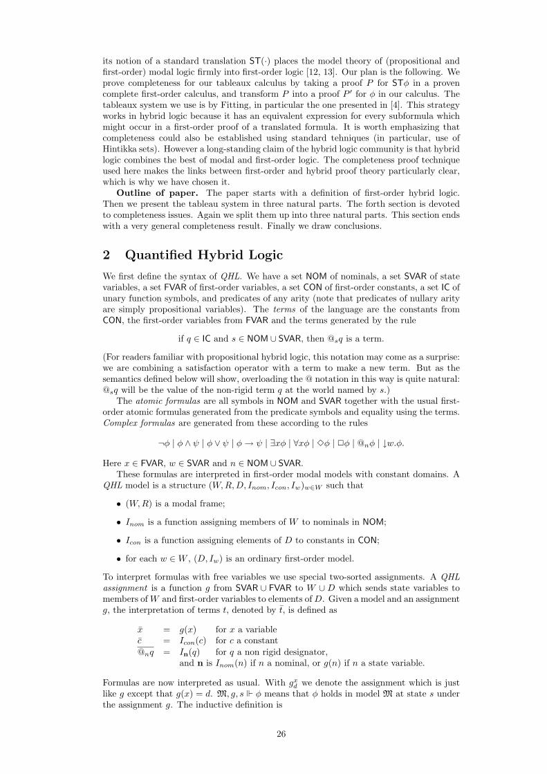
its notion of a standard translation ST(·) places the model theory of (propositional andfirst-order) modal logic firmly into first-order logic [12, 13]. Our plan is the following. Weprove completeness for our tableaux calculus by taking a proof P for STφ in a provencomplete first-order calculus, and transform P into a proof P ′ for φ in our calculus. Thetableaux system we use is by Fitting, in particular the one presented in [4]. This strategyworks in hybrid logic because it has an equivalent expression for every subformula whichmight occur in a first-order proof of a translated formula. It is worth emphasizing thatcompleteness could also be established using standard tehniques (in particular, use ofHintikka sets). However a long-standing claim of the hybrid logic community is that hybridlogic combines the best of modal and first-order logic. The completeness proof techniqueused here makes the links between first-order and hybrid proof theory particularly clear,which is why we have chosen it.

Outline of paper. The paper starts with a definition of first-order hybrid logic.Then we present the tableau system in three natural parts. The forth section is devotedto completeness issues. Again we split them up into three natural parts. This section endswith a very general completeness result. Finally we draw conclusions.

2 Quantified Hybrid Logic

We first define the syntax of QHL. We have a set NOM of nominals, a set SVAR of statevariables, a set FVAR of first-order variables, a set CON of first-order constants, a set IC ofunary function symbols, and predicates of any arity (note that predicates of nullary arityare simply propositional variables). The terms of the language are the constants fromCON, the first-order variables from FVAR and the terms generated by the rule

if q ∈ IC and s ∈ NOM ∪ SVAR, then @sq is a term.

(For readers familiar with propositional hybrid logic, this notation may come as a surprise:we are combining a satisfaction operator with a term to make a new term. But as thesemantics defined below will show, overloading the @ notation in this way is quite natural:@sq will be the value of the non-rigid term q at the world named by s.)

The atomic formulas are all symbols in NOM and SVAR together with the usual first-order atomic formulas generated from the predicate symbols and equality using the terms.Complex formulas are generated from these according to the rules

¬φ | φ ∧ ψ | φ ∨ ψ | φ→ ψ | ∃xφ | ∀xφ | 3φ | 2φ | @nφ | ↓w.φ.

Here x ∈ FVAR, w ∈ SVAR and n ∈ NOM ∪ SVAR.These formulas are interpreted in first-order modal models with constant domains. A

QHL model is a structure (W,R,D, Inom, Icon, Iw)w∈W such that

• (W,R) is a modal frame;

• Inom is a function assigning members of W to nominals in NOM;

• Icon is a function assigning elements of D to constants in CON;

• for each w ∈W , (D, Iw) is an ordinary first-order model.

To interpret formulas with free variables we use special two-sorted assignments. A QHLassignment is a function g from SVAR ∪ FVAR to W ∪ D which sends state variables tomembers ofW and first-order variables to elements ofD. Given a model and an assignmentg, the interpretation of terms t, denoted by t, is defined as

x = g(x) for x a variablec = Icon(c) for c a constant@nq = In(q) for q a non rigid designator,

and n is Inom(n) if n a nominal, or g(n) if n a state variable.

Formulas are now interpreted as usual. With gxd we denote the assignment which is just

like g except that g(x) = d. M, g, s φ means that φ holds in model M at state s underthe assignment g. The inductive definition is

26

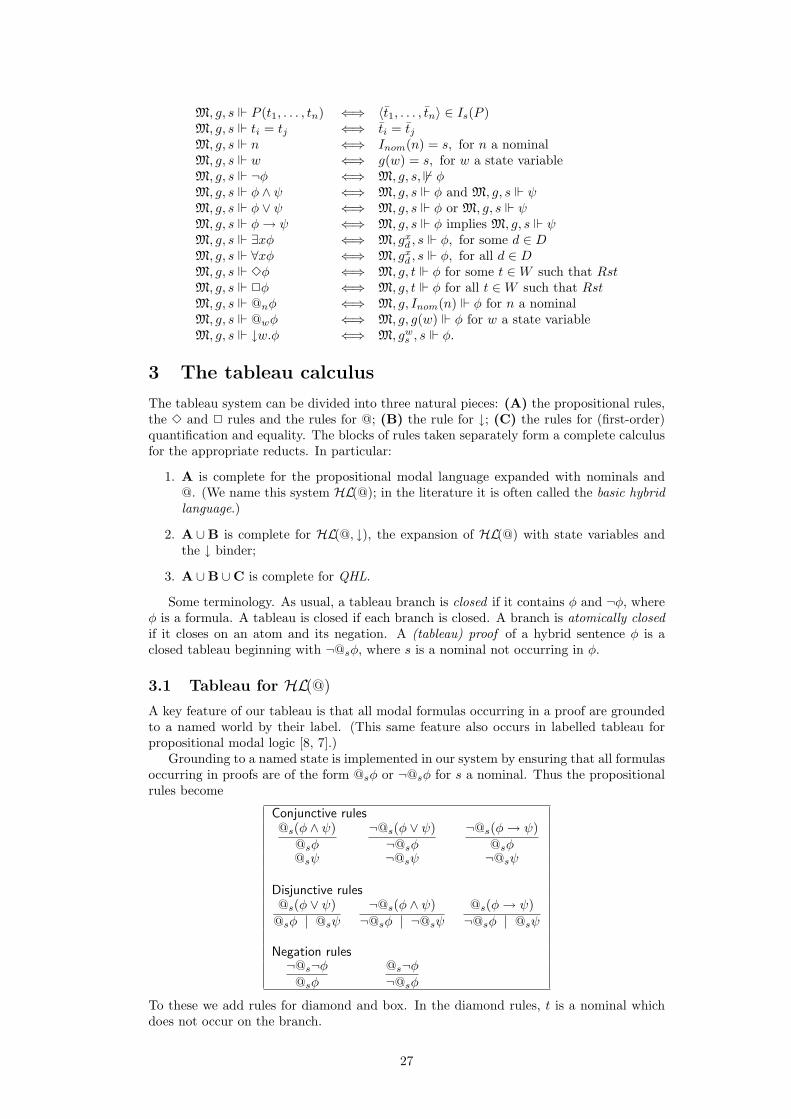
M, g, s P (t1, . . . , tn) ⇐⇒ 〈t1, . . . , tn〉 ∈ Is(P )M, g, s ti = tj ⇐⇒ ti = tjM, g, s n ⇐⇒ Inom(n) = s, for n a nominalM, g, s w ⇐⇒ g(w) = s, for w a state variableM, g, s ¬φ ⇐⇒ M, g, s, 6 φM, g, s φ ∧ ψ ⇐⇒ M, g, s φ and M, g, s ψM, g, s φ ∨ ψ ⇐⇒ M, g, s φ or M, g, s ψM, g, s φ→ ψ ⇐⇒ M, g, s φ implies M, g, s ψM, g, s ∃xφ ⇐⇒ M, gx

d , s φ, for some d ∈ DM, g, s ∀xφ ⇐⇒ M, gx

d , s φ, for all d ∈ DM, g, s 3φ ⇐⇒ M, g, t φ for some t ∈W such that RstM, g, s 2φ ⇐⇒ M, g, t φ for all t ∈W such that RstM, g, s @nφ ⇐⇒ M, g, Inom(n) φ for n a nominalM, g, s @wφ ⇐⇒ M, g, g(w) φ for w a state variableM, g, s ↓w.φ ⇐⇒ M, gw

s , s φ.

3 The tableau calculus

The tableau system can be divided into three natural pieces: (A) the propositional rules,the 3 and 2 rules and the rules for @; (B) the rule for ↓; (C) the rules for (first-order)quantification and equality. The blocks of rules taken separately form a complete calculusfor the appropriate reducts. In particular:

1. A is complete for the propositional modal language expanded with nominals and@. (We name this system HL(@); in the literature it is often called the basic hybridlanguage.)

2. A ∪B is complete for HL(@, ↓), the expansion of HL(@) with state variables andthe ↓ binder;

3. A ∪B ∪C is complete for QHL.

Some terminology. As usual, a tableau branch is closed if it contains φ and ¬φ, whereφ is a formula. A tableau is closed if each branch is closed. A branch is atomically closedif it closes on an atom and its negation. A (tableau) proof of a hybrid sentence φ is aclosed tableau beginning with ¬@sφ, where s is a nominal not occurring in φ.

3.1 Tableau for HL(@)

A key feature of our tableau is that all modal formulas occurring in a proof are groundedto a named world by their label. (This same feature also occurs in labelled tableau forpropositional modal logic [8, 7].)

Grounding to a named state is implemented in our system by ensuring that all formulasoccurring in proofs are of the form @sφ or ¬@sφ for s a nominal. Thus the propositionalrules become

Conjunctive rules@s(φ ∧ ψ)

@sφ

¬@s(φ ∨ ψ)¬@sφ

¬@s(φ→ ψ)@sφ

@sψ ¬@sψ ¬@sψ

Disjunctive rules@s(φ ∨ ψ)

@sφ | @sψ

¬@s(φ ∧ ψ)¬@sφ | ¬@sψ

@s(φ→ ψ)¬@sφ | @sψ

Negation rules¬@s¬φ

@sφ

@s¬φ¬@sφ

To these we add rules for diamond and box. In the diamond rules, t is a nominal whichdoes not occur on the branch.

27

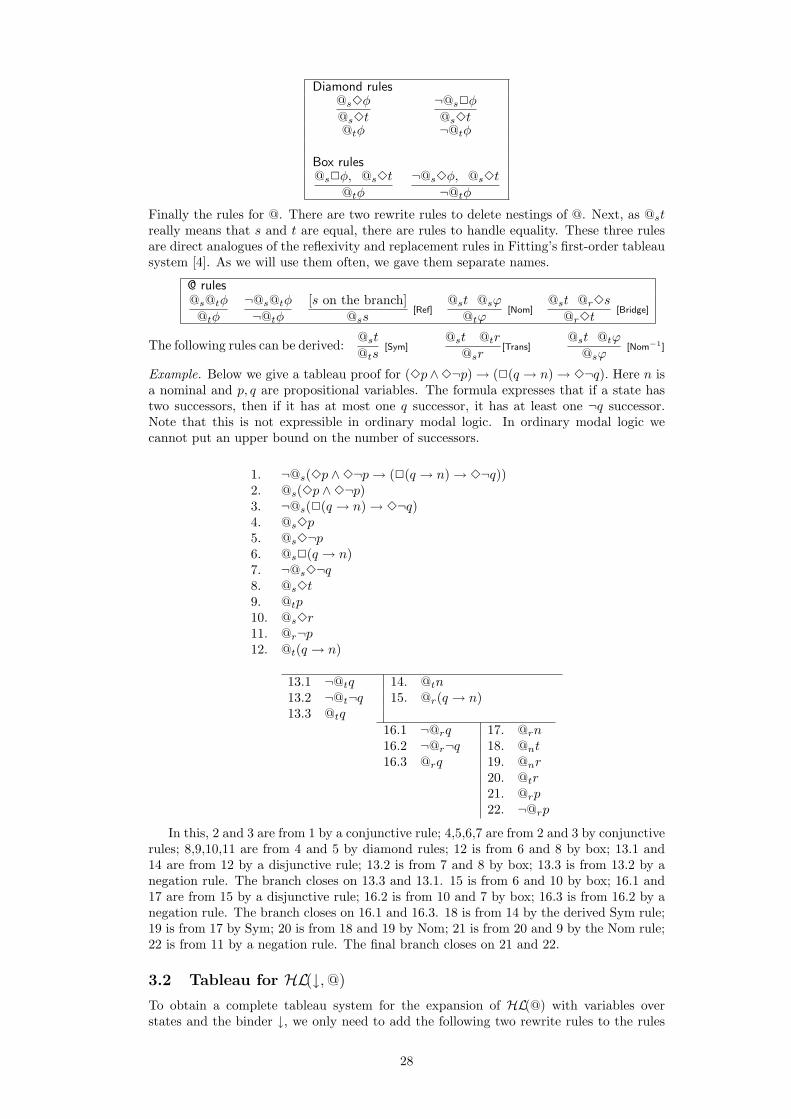
Diamond rules@s3φ

@s3t

¬@s2φ

@s3t@tφ ¬@tφ

Box rules@s2φ, @s3t

@tφ

¬@s3φ, @s3t

¬@tφ

Finally the rules for @. There are two rewrite rules to delete nestings of @. Next, as @streally means that s and t are equal, there are rules to handle equality. These three rulesare direct analogues of the reflexivity and replacement rules in Fitting’s first-order tableausystem [4]. As we will use them often, we gave them separate names.

@ rules@s@tφ

@tφ

¬@s@tφ

¬@tφ

[s on the branch]@ss

[Ref]@st @sϕ

@tϕ[Nom]

@st @r3s

@r3t[Bridge]

The following rules can be derived:@st

@ts[Sym]

@st @tr

@sr[Trans]

@st @tϕ

@sϕ[Nom−1]

Example. Below we give a tableau proof for (3p∧3¬p)→ (2(q → n)→ 3¬q). Here n isa nominal and p, q are propositional variables. The formula expresses that if a state hastwo successors, then if it has at most one q successor, it has at least one ¬q successor.Note that this is not expressible in ordinary modal logic. In ordinary modal logic wecannot put an upper bound on the number of successors.

1. ¬@s(3p ∧3¬p→ (2(q → n)→ 3¬q))2. @s(3p ∧3¬p)3. ¬@s(2(q → n)→ 3¬q)4. @s3p5. @s3¬p6. @s2(q → n)7. ¬@s3¬q8. @s3t9. @tp10. @s3r11. @r¬p12. @t(q → n)

13.1 ¬@tq 14. @tn13.2 ¬@t¬q 15. @r(q → n)13.3 @tq

16.1 ¬@rq 17. @rn16.2 ¬@r¬q 18. @nt16.3 @rq 19. @nr

20. @tr21. @rp22. ¬@rp

In this, 2 and 3 are from 1 by a conjunctive rule; 4,5,6,7 are from 2 and 3 by conjunctiverules; 8,9,10,11 are from 4 and 5 by diamond rules; 12 is from 6 and 8 by box; 13.1 and14 are from 12 by a disjunctive rule; 13.2 is from 7 and 8 by box; 13.3 is from 13.2 by anegation rule. The branch closes on 13.3 and 13.1. 15 is from 6 and 10 by box; 16.1 and17 are from 15 by a disjunctive rule; 16.2 is from 10 and 7 by box; 16.3 is from 16.2 by anegation rule. The branch closes on 16.1 and 16.3. 18 is from 14 by the derived Sym rule;19 is from 17 by Sym; 20 is from 18 and 19 by Nom; 21 is from 20 and 9 by the Nom rule;22 is from 11 by a negation rule. The final branch closes on 21 and 22.

3.2 Tableau for HL(↓, @)

To obtain a complete tableau system for the expansion of HL(@) with variables overstates and the binder ↓, we only need to add the following two rewrite rules to the rules

28

for HL(@):

Downarrow rules@s↓w.φ

@sφ[s/w]¬@s↓w.φ¬@sφ[s/w]

Here [s/w] means substitute s for all free occurrences of w in φ. Because s is always anominal, whence cannot be quantified over, we do not have to worry about accidentalbindings. As an example the reader can try to prove the validities ↓w.3w → (p → 3p)and ↓w.23w → (32p→ p).

3.3 Tableau for QHL

A complete tableau system for quantified hybrid logic consists of the HL(↓,@) system,plus the (adjusted) rules for the quantifiers and equality from Fitting’s system (see [4])for first-order logic with equality, plus two rules relating equalities across worlds. In theexistential rules, c is a parameter which is new to the branch. As parameters are neverquantified over, the substitution [c/x] is free for the formula φ(x). In the universal rules,t is any grounded term on the branch (thus either a first-order constant, a parameter ora grounded definite description). A grounded definite description is a term @nq for n anominal and q a non-rigid designator from IC.

Existential rules@s∃xφ(x)@sφ(c)

¬@s∀xφ(x)¬@sφ(c)

Universal rules@s∀xφ(x)

@sφ(t)¬@s∃xφ(x)¬@sφ(t)

Besides Fitting’s [4] Reflexivity (Ref) and Replacement (RR) rules, there are three extrarules for equality. The first (called DD) states that if n and m denote the same state,then @nq and @mq denote the same individual. The second and third (both called @=)embody that equality is a rigid predicate: if two terms are the same in one world, theyare the same in every world. Because these two rules peel the leading @n off equalities,reflexivity and replacement can be kept in the old format.

QHL Equality rules

t = t[Ref]

t = u, φ(t)φ[u] [RR],

@nm

@nq = @mq[DD]

@n(ti = tj)ti = tj

[@=]¬@n(ti = tj)¬(ti = tj)

[@=]

In the Replacement rule, φ[u] denotes φ(t) with some of the occurrences of t replaced byu.

Example. The most interesting examples deal with equality and rigid and non-rigiddesignators. Consider the sentence Caroline is Miss America. When formalising thislet c be a rigid designator denoting Caroline and q a non-rigid designator denoting MissAmerica. Then ↓x.(c = @xq) means Caroline is the present Miss America. It is true in astate w if Icon(c) = Iw(q). This formula has the following relation with the 2 operator:

6|= (↓w.c = @wq) → 2↓w.c = @wq (1)|= (↓w.c = @wq) → ↓w.2c = @wq. (2)

A falsifying model for the sentence in (1) is given by two worlds n and m, with Rnm,and a domain {a, b} with the interpretation Icon(c) = In(q) = a and Im(q) = b. Then (1)fails at world n. When downarrow has wide scope in the consequent, the formula becomes

29

true. Here is the tableau proof:

1. ¬@n((↓w.c = @wq)→ ↓w.2(c = @wq))2. @n↓w.c = @wq3. ¬@n↓w.2(c = @wq)4. @n(c = @nq)5. ¬@n2(c = @nq)6. @n3m7. ¬@m(c = @nq)8. c = @nq9. ¬(c = @nq).

In this, 2 and 3 are from 1 by a conjunctive rule; 4 and 5 are from 2 and3 by a downarrow rule, respectively; 6 and 7 are from 5 by a diamondrule; 8 and 9 are from 4 and 7 by an @= rule, respectively.

4 Soundness and Completeness

The argument to establish soundness follows the familiar pattern: show that satisfiabilityis preserved by each tableau rule application. This is easy to check and left to the reader.Completeness will be established using the standard translation and a complete first-order inference system. We use the system that is closest to the one presented here: thetableau calculus for first-order logic with equality from Fitting [4] with the reflexivity andreplacement rules (restricted to atoms). The main line of the argument is the following. Weneed to establish that every valid QHL sentence has a QHL tableau proof. The standardtranslation preserves validity, thus a QHL sentence φ is valid if and only if the first-ordersentence STφ is valid. For valid STφ, there exists a closed first-order tableau proof Tstarting with ¬STφ. Our task is to transform this closed first-order proof T starting with¬STφ into a closed QHL tableau proof T ′ starting with ¬φ.

Most of the work concerns the modalities and the @ operator, because with these thestandard translation creates the largest change in syntactic structure. For this reason wepresent the completeness proof for the simplest logic HL(@) separately. After that, therest will be easy.

Before we can continue we have to settle two things. We change Fitting’s first-ordertableau rules a little bit in order to better cope with translations of modal formulas.Besides that we have to use a modified translation. We start with the former.

In order to save on inductive proofs and definitions, we assume fror now on that theQHL language contains as primitive logical operators only ¬,∧,2,@s, ↓w. and ∀v. Clearlythis is without loss of generality because the other operators can be defined in terms ofthese.

4.1 Tableau rules for relativized quantifiers

The translation of a box modality yields a relativized universal formula of the form∀x(A(x) → C(x)), with A(x) an atom. For these relativized universals, a more effi-cient tableau rule exists than the combination of universal and → rule together. In fact itis nothing but Modes Ponens. For t a closed term,

Modes Ponens (MP)A(t), ∀x(A(x)→ φ(x))

φ(t)A(t), ¬∃x(A(x) ∧ φ(x))

¬φ(t)

We change Fitting’s calculus such that on universals relativized by an atom the normaluniversal rules cannot be applied, but MP can. This is easily seen to be complete (cfalso [11]. We can make a further reduction in complexity in the case the antecedent isan equality. Then the statement just expresses a substitution. We also add the followingrules to Fitting’s calculus and make the proviso that universal and existential rules arenever applied to quantified sentences relativized by an equality.

Substitution Rules∀x(x = t→ φ(x))

φ(t)∃x(x = t ∧ φ(x))

φ(t)¬∀x(x = t→ φ(x))

¬φ(t)¬∃x(x = t ∧ φ(x))

¬φ(t)

30

4.2 Translation using predicate abstraction

Unfortunately, the usual standard translation does not square well with the intention tochange one proof into another. Though it is truth preserving, it does not preserve syntacticstructure. Because we want to transform a proof for the translation of φ into a proof forφ, we need to translate backwards as well. It is crucial that applying the backwardstranslation to the translation of φ yields φ again. This is simply not obtainable by thestandard translation or obvious variants.

An example might explain why not. We can read @s(p ∧ q) as saying that state s hasthe property p∧ q. As we want to translate proposition letters to one place predicates, infirst-order logic we can only say then that s has property p and s has property q. This isof course logically equivalent, but syntactically different. We would like to have machinerywhich can turn formulas into predicates, so that we can speak about the property “p andq”. The lambda calculus provides precisely this: 〈λx.(Px ∧ Qx)〉 denotes the propertyof being P and Q. The formula 〈λx.(Px ∧ Qx)〉(s) serves then as an excellent proxy for@s(p ∧ q).

We add predicate abstraction to the language. This will only be defined for variablesranging over individuals. Thus we only add a piece of syntactic sugar. The expressivepower of the language remains the same, it is just first-order logic. For a thorough intro-duction to real predicate abstraction in modal logic we refer to [6].

Suppose φ is a first-order formula and x a first-order variable. Then 〈λx.φ〉 is a pred-icate abstract. Its free variable occurrences are the free variable occurrences of φ exceptfor x. Predicate abstracts behave as unary predicate symbols; new atomic formulas frompredicate abstracts 〈λx.φ〉 can be made by the rule

if t is a term, then 〈λx.φ〉(t) is a formula.

Examples are 〈λx.Px〉(t) and 〈λx.Px ∧ Qx〉(s). The new formulas get their meaning byperforming β-reduction:

the β-reduction of 〈λx.φ〉(t) is φ[t/x].

The meaning of 〈λx.φ〉(t) is simply the meaning of φ[t/x]. This shows that the expressivepower remains the same. Our convention is that in λ expressions, the . takes wide scope,thus 〈λx.φ ∧ ψ〉 = 〈λx.(φ ∧ ψ)〉.

In order to handle predicate abstracts in tableau proofs, we need only add two verysimple rules to Fitting’s system. The rules just implement β-reduction. Here they are

Abstract rules〈λx.φ〉(t)φ[t/x]

¬〈λx.φ〉(t)¬φ[t/x]

Fitting’s tableau system with the two abstract rules added is a complete inference sys-tem for the expansion of first-order logic with λ abstraction with variables ranging overindividuals [5].

We are ready to define the new standard translation AT for the propositional hybridlanguage, together with its inverse AT−. In a certain sense, this translation can be tracedback to the paper [9] in which McCarthy and Hayes introduce the situation calculus.AT y(φ) and AT−

y (φ) are defined in the same way but with x and y interchanged, e.g.,AT y(p) := Py and AT y(2φ) := 〈λy.∀x(Ryx→ ATx(φ))〉(y).

ATx(p) := PxATx(n) := x = nATx(¬φ) := 〈λx.¬ATx(φ)〉(x)ATx(φ ∧ ψ) := 〈λx.ATx(φ) ∧ATx(ψ)〉(x)ATx(2φ) := 〈λx.∀y(Rxy → AT y(φ))〉(x)ATx(@nφ) := 〈λx.∀x(x = n→ ATx(φ))〉(x)

AT−x (Px) := p

AT−x (x = n) := n

AT−x (〈λx.¬φ〉(x)) := ¬AT−

x (φ)AT−

x (〈λx.φ ∧ ψ〉(x)) := AT−x (φ) ∧AT−

x (ψ)AT−

x (〈λx.∀y(Rxy → φ)〉(x)) := 2AT−y (φ)

AT−x (〈λx.∀x(x = n→ φ)〉(x)) := @nAT−

x (φ)

31

The following properties of AT and AT− hold, for every HL(@) formula φ,

ATx(φ) is always a formula of the form 〈λx.ψ〉(x) or Px or x = n. (3)AT−

x (ATx(φ)) = φ, and similarly when x is replaced by y. (4)φ is HL(@) valid iff ATx(φ) is first-order valid. (5)

(3) follows from the definition. (4) is proved by induction on the complexity of the HL(@)formula. (5) is immediate by performing β-reduction and the well-known result on thestandard translation.

4.3 Completeness for HL(@)

We now specify an algorithm for turning a closed Fitting tableau for the formulaATx(φ)[c/x] (where c is a parameter) into a closed HL(@) tableau for @cφ. Some termi-nology will be useful. A literal is a grounded formula of the form

P (t) | t = u | Rtu | 〈λx.φ〉(t) | 〈λy.φ〉(t), or its negation.

Define the following translation (·)∗ from positive literals to HL(@) sentences

P (t)∗ := @tp(t = u)∗ := @tu(Rtu)∗ := @t3u

(〈λx.φ〉(t))∗ := @tAT−x (〈λx.φ〉(x))

(〈λy.φ〉(t))∗ := @tAT−y (〈λy.φ〉(y)).

For negative literals (¬φ), we set (¬φ)∗ = ¬φ∗.We recapitulate: AT translates a hybrid formula into a first-order formula and AT−

translates them backwards. The translation (·)∗ translates literals occurring in a first-order tableau proof to hybrid formulas. Note that these literals may contain parametersintroduced in the proof. The crucial connection between the forward and backward trans-lations is that they preserve syntactic structure: for φ a hybrid formula and t a nominalor parameter,

(ATx(φ)[t/x])∗ = @tφ and (¬ATx(φ)[t/x])∗ = ¬@tφ. (6)

Property (6) follows immediately from the definition of (·)∗ and (4).

We are ready to specify the algorithm. Let T be a closed Fitting tableau for the formulaATx(φ)[c/x]. Without loss of generality we may assume that T is atomically closed. LetT ′ simply be T with all literals replaced by their (·)∗ translation and all other formulasremoved.

Claim T ′ is HL(@) tableau proof for φ.

We first observe that T ′ starts with ¬@cφ. This is because T starts with the literal¬ATx(φ)[c/x] whose ∗ translation is ¬@cφ by (6).

Secondly, every branch in T ′ closes. This is because T branches close on literals, whichwe all move over to T ′, keeping the negation signs in place.

Finally we show that T ′ is a correct HL(@) tableau. We prove this by showing thatevery application of rules to a literal l in T can be matched by an application of a (derived)rule to l∗ in T ′. More precisely, for every literal l in T , for all literals l1, l2 produced froml by applying rules, the literals l∗1, l

∗2 can be obtained from l∗ by applying a (derived) rule

in T ′.We do a case-analysis according to the structure of the literals. By the translation

we know that every literal which is a λ-formula has the form 〈λz.AT z(ψ)〉(t), for z eitherx or y, and ψ an HL(@) formula. After performing β-reduction we obtain AT z(ψ)[t/z]whose (·)∗ translation is @tψ by (6). The case analysis is presented for the connectivesin Table 2. This table is read as follows. On the left are first-order proofs with smallannotations indicating which rule is applied on what to obtain the result. On the right arethe HL(@) proofs which derive the (·)∗ translated results from the (·)∗ translated premises,again annotated.

32

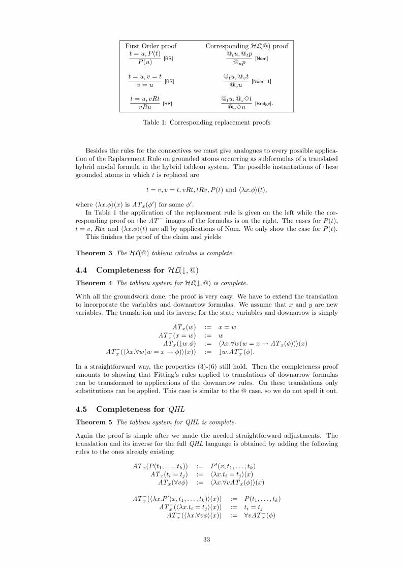
First Order proof Corresponding HL(@) prooft = u, P (t)P (u) [RR]

@tu,@tp

@up[Nom]

t = u, v = t

v = u[RR]

@tu,@vt

@vu[Nom−1]

t = u, vRt

vRu[RR]

@tu,@v3t

@v3u[Bridge].

Table 1: Corresponding replacement proofs

Besides the rules for the connectives we must give analogues to every possible applica-tion of the Replacement Rule on grounded atoms occurring as subformulas of a translatedhybrid modal formula in the hybrid tableau system. The possible instantiations of thesegrounded atoms in which t is replaced are

t = v, v = t, vRt, tRv, P (t) and 〈λx.φ〉(t),

where 〈λx.φ〉(x) is ATx(φ′) for some φ′.In Table 1 the application of the replacement rule is given on the left while the cor-

responding proof on the AT− images of the formulas is on the right. The cases for P (t),t = v, Rtv and 〈λx.φ〉(t) are all by applications of Nom. We only show the case for P (t).

This finishes the proof of the claim and yields

Theorem 3 The HL(@) tableau calculus is complete.

4.4 Completeness for HL(↓, @)

Theorem 4 The tableau system for HL(↓,@) is complete.

With all the groundwork done, the proof is very easy. We have to extend the translationto incorporate the variables and downarrow formulas. We assume that x and y are newvariables. The translation and its inverse for the state variables and downarrow is simply

ATx(w) := x = wAT−

x (x = w) := wATx(↓w.φ) := 〈λx.∀w(w = x→ ATx(φ))〉(x)

AT−x (〈λx.∀w(w = x→ φ)〉(x)) := ↓w.AT−

x (φ).

In a straightforward way, the properties (3)-(6) still hold. Then the completeness proofamounts to showing that Fitting’s rules applied to translations of downarrow formulascan be transformed to applications of the downarrow rules. On these translations onlysubstitutions can be applied. This case is similar to the @ case, so we do not spell it out.

4.5 Completeness for QHL

Theorem 5 The tableau system for QHL is complete.

Again the proof is simple after we made the needed straightforward adjustments. Thetranslation and its inverse for the full QHL language is obtained by adding the followingrules to the ones already existing:

ATx(P (t1, . . . , tk)) := P ′(x, t1, . . . , tk)ATx(ti = tj) := 〈λx.ti = tj〉(x)

ATx(∀vφ) := 〈λx.∀vATx(φ)〉(x)

AT−x (〈λx.P ′(x, t1, . . . , tk)〉(x)) := P (t1, . . . , tk)

AT−x (〈λx.ti = tj〉(x)) := ti = tj

AT−x (〈λx.∀vφ〉(x)) := ∀vAT−

x (φ)

33

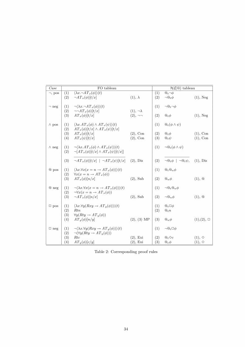
Case FO tableau HL(@) tableau

¬, pos (1) 〈λx.¬ATx(φ)〉(t) (1) @t¬φ(2) ¬ATx(φ)[t/x] (1), λ (2) ¬@tφ (1), Neg

¬ neg (1) ¬〈λx.¬ATx(φ)〉(t) (1) ¬@t¬φ(2) ¬¬ATx(φ)[t/x] (1), ¬λ(3) ATx(φ)[t/x] (2), ¬¬ (2) @tφ (1), Neg

∧ pos (1) 〈λx.ATx(φ) ∧ATx(ψ)〉(t) (1) @t(φ ∧ ψ)(2) ATx(φ)[t/x] ∧ATx(ψ)[t/x](3) ATx(φ)[t/x] (2), Con (2) @tφ (1), Con(4) ATx(ψ)[t/x] (2), Con (3) @tψ (1), Con

∧ neg (1) ¬〈λx.ATx(φ) ∧ATx(ψ)〉(t) (1) ¬@t(φ ∧ ψ)(2) ¬[ATx(φ)[t/x] ∧ATx(ψ)[t/x]]

(3) ¬ATx(φ)[t/x] | ¬ATx(ψ)[t/x] (2), Dis (2) ¬@tφ | ¬@tψ, (1), Dis

@ pos (1) 〈λx.∀x(x = n→ ATx(φ))〉(t) (1) @t@nφ(2) ∀x(x = n→ ATx(φ))(3) ATx(φ)[n/x] (2), Sub (2) @nφ (1), @

@ neg (1) ¬〈λx.∀x(x = n→ ATx(φ))〉(t) (1) ¬@t@nφ(2) ¬∀x(x = n→ ATx(φ))(3) ¬ATx(φ)[n/x] (2), Sub (2) ¬@nφ (1), @

2 pos (1) 〈λx.∀y(Rxy → AT y(φ))〉(t) (1) @t2φ(2) Rtn (2) @tn(3) ∀y(Rty → AT y(φ))(4) AT y(φ)[n/y] (2), (3) MP (3) @nφ (1),(2), 2

2 neg (1) ¬〈λx.∀y(Rxy → AT y(φ))〉(t) (1) ¬@t2φ(2) ¬(∀y(Rty → AT y(φ)))(3) Rtc (2), Exi (2) @t3c (1), 3

(4) AT y(φ)[c/y] (2), Exi (3) @cφ (1), 3

Table 2: Corresponding proof rules

34

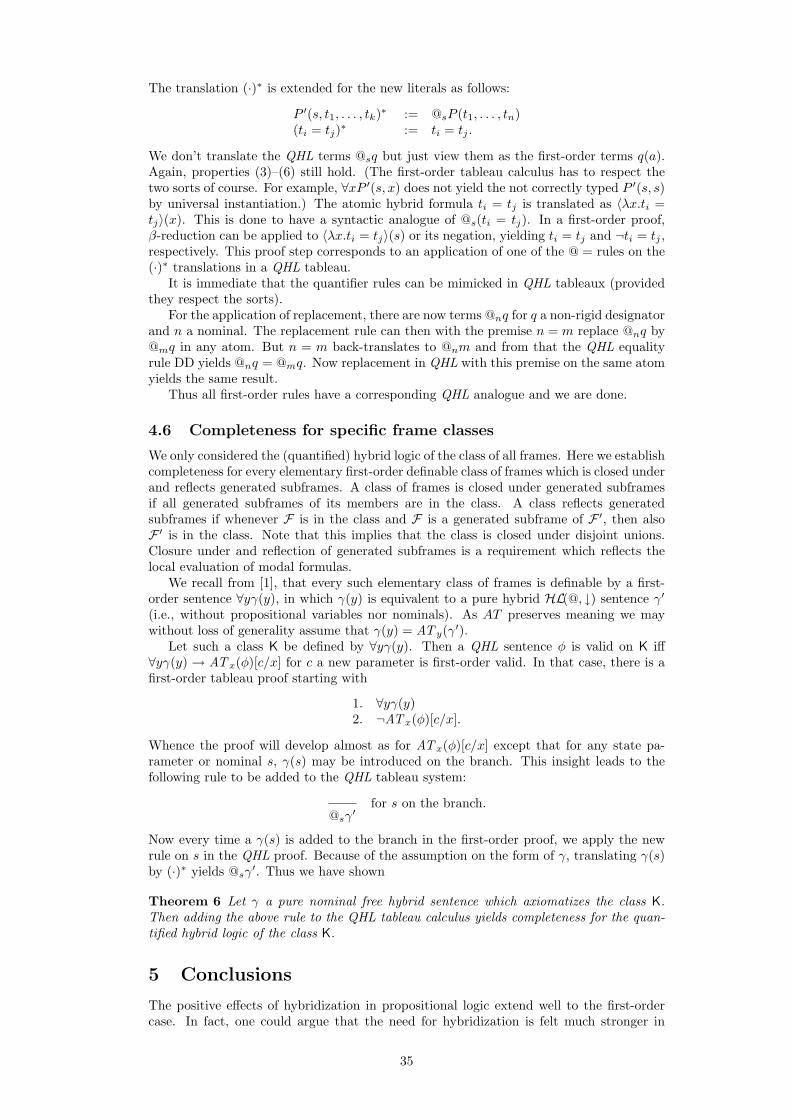
The translation (·)∗ is extended for the new literals as follows:

P ′(s, t1, . . . , tk)∗ := @sP (t1, . . . , tn)(ti = tj)∗ := ti = tj .

We don’t translate the QHL terms @sq but just view them as the first-order terms q(a).Again, properties (3)–(6) still hold. (The first-order tableau calculus has to respect thetwo sorts of course. For example, ∀xP ′(s, x) does not yield the not correctly typed P ′(s, s)by universal instantiation.) The atomic hybrid formula ti = tj is translated as 〈λx.ti =tj〉(x). This is done to have a syntactic analogue of @s(ti = tj). In a first-order proof,β-reduction can be applied to 〈λx.ti = tj〉(s) or its negation, yielding ti = tj and ¬ti = tj ,respectively. This proof step corresponds to an application of one of the @ = rules on the(·)∗ translations in a QHL tableau.

It is immediate that the quantifier rules can be mimicked in QHL tableaux (providedthey respect the sorts).

For the application of replacement, there are now terms @nq for q a non-rigid designatorand n a nominal. The replacement rule can then with the premise n = m replace @nq by@mq in any atom. But n = m back-translates to @nm and from that the QHL equalityrule DD yields @nq = @mq. Now replacement in QHL with this premise on the same atomyields the same result.

Thus all first-order rules have a corresponding QHL analogue and we are done.

4.6 Completeness for specific frame classes

We only considered the (quantified) hybrid logic of the class of all frames. Here we establishcompleteness for every elementary first-order definable class of frames which is closed underand reflects generated subframes. A class of frames is closed under generated subframesif all generated subframes of its members are in the class. A class reflects generatedsubframes if whenever F is in the class and F is a generated subframe of F ′, then alsoF ′ is in the class. Note that this implies that the class is closed under disjoint unions.Closure under and reflection of generated subframes is a requirement which reflects thelocal evaluation of modal formulas.

We recall from [1], that every such elementary class of frames is definable by a first-order sentence ∀yγ(y), in which γ(y) is equivalent to a pure hybrid HL(@, ↓) sentence γ′

(i.e., without propositional variables nor nominals). As AT preserves meaning we maywithout loss of generality assume that γ(y) = AT y(γ′).

Let such a class K be defined by ∀yγ(y). Then a QHL sentence φ is valid on K iff∀yγ(y) → ATx(φ)[c/x] for c a new parameter is first-order valid. In that case, there is afirst-order tableau proof starting with

1. ∀yγ(y)2. ¬ATx(φ)[c/x].

Whence the proof will develop almost as for ATx(φ)[c/x] except that for any state pa-rameter or nominal s, γ(s) may be introduced on the branch. This insight leads to thefollowing rule to be added to the QHL tableau system:

@sγ′

for s on the branch.

Now every time a γ(s) is added to the branch in the first-order proof, we apply the newrule on s in the QHL proof. Because of the assumption on the form of γ, translating γ(s)by (·)∗ yields @sγ

′. Thus we have shown

Theorem 6 Let γ a pure nominal free hybrid sentence which axiomatizes the class K.Then adding the above rule to the QHL tableau calculus yields completeness for the quan-tified hybrid logic of the class K.

5 Conclusions

The positive effects of hybridization in propositional logic extend well to the first-ordercase. In fact, one could argue that the need for hybridization is felt much stronger in

35

first-order modal logic. The field is plagued with failures of desirable properties, andconsequently more difficult and obscure than its propositional counterpart. Here we havepresented an extremely general completeness theorem (Theorem 6) covering virtually allmodally interesting elementary frame classes. In a companion paper we have shown thatthe presented calculus can be used to construct interpolants. Interpolation is one of theproperties which fail in many quantified modal logics. This theorem also extends to allframe classes from Theorem 6. These very general results indicate that the additions tothe syntax are natural and extremely useful.

The paper contained two important results. First of all, the proof method for showingcompleteness. The standard translation was used in a non-trivial way to transfer a first-order result into the modal setting. In the hybrid language, this was particularly easy, as itcontains such first-order proof-elements as parameters. We wonder if the translation usingλ-abstraction could also be used to obtain completeness of traditional tableau systems.We think this is an important research direction. Too many proofs are repeated over andover with tiny changes in modal logic. Maybe hybridization is needed to change modallogic into a field in which results are recycled instead of proofs. It’s worth the price.

The second important result is our treatment of definite descriptions like Miss Amer-ica.In QHL it is not possible to write intensional terms as in Montague’s IL. The hiddenvariables in intensional terms cause many technical problems and make IL mathematicallycomplicated. The use of @ to ground non-rigid designators to states is a simple remedy.

References

[1] C. Areces, P. Blackburn, and M. Marx. Hybrid logics: Characterization, interpolationand complexity. Journal of Symbolic Logic, 66(3):977–1010, 2001.

[2] C. Areces, P. Blackburn, and M. Marx. Repairing the interpolation lemma in quan-tified modal logic. Report PP–2001–19, ILLC. To appear in Annals of Pure andApplied Logic.

[3] K. Fine. Failures of the interpolation lemma in quantified modal logic. Journal ofSymbolic Logic, 44(2):201–206, 1979.

[4] M. Fitting. First Order Logic and Automated Theorem Proving (second edition).Springer Verlag, 1996.

[5] M. Fitting. Types, Tableaus, and Godel’s God. Unpublished Draft, 1999.

[6] M. Fitting and R. Mendelsohn. First–Order Modal Logic. Kluwer, 1998.

[7] D. Gabbay. Labelled Deductive Systems. Oxford University Press, 1996.

[8] R. Gore. Tableau methods for modal and temporal logics. In M D’Agostino,et aleditors, Handbook of Tableau Methods, pages 297–396. Kluwer Academic Publishers,1999.

[9] John McCarthy and Patrick J. Hayes. Some philosophical problems from the stand-point of artificial intelligence. In B. Meltzer and D. Michie, editors, Machine Intelli-gence 4, pages 463–502. Edinburgh University Press, 1969.

[10] J. Seligman. Internalization: The case of hybrid logic. Journal of Logic and Compu-tation, 11(5):671–689, 2001.

[11] R. Smullyan. First Order Logic. Springer–Verlag, 1968.

[12] J. van Benthem. Modal Logic and Classical Logic. Bibliopolis, Naples, 1983.

[13] J. van Benthem. Correspondence theory. In D.M. Gabbay and F. Guenther, editors,Handbook of Philosophical Logic, volume 2, pages 167–248. Reidel, Dordrecht, 1984.

36

Beyond Pure Axioms:

Node Creating Rules in Hybrid Tableaux2

(DRAFT VERSION)

Patrick Blackburn Balder ten CateINRIA Lorraine ILLC, Universiteit van Amsterdam615, rue du Jardin Botanique Nieuwe Doelenstraat 1554602 Villers les Nancy Cedex, France 1012CP Amsterdam, NetherlandsEmail: patrick@aplog.org Email: b.ten.cate@hum.uva.nl

Abstract

We present a method of extending the tableau calculus for the basic hybrid lan-guage which automatically yields completeness results for many frame classes thatcannot be defined by means of pure axioms (for example, Church-Rosser frames).The extended calculus makes use of node-creating rules. These rules trade on theidea of using nominals to perform skolemization on formulas of the strong hybrid lan-guage. Alternatively, viewing them from a Hilbert-style perspective, such rules canbe viewed as a systematic generalization of Gabbay’s rules for the undefinable. Ourtableau complexness result covers all frame classes definable by pure nominal-freeuniversal existential sentences of the strong hybrid language. This properly includesall frame classes definable by universal existential first-order sentences.

1 Basic Hybrid Logic

Basic hybrid logic is the result of extending modal logic with nominals and the @-operator.Suppose we are given a set σ of modalities, and two (countably infinite) disjoint setsPROP (whose elements are typically written p, q, and r, possibly subscripted, and calledproposition letters) and NOM (whose elements are typically written i, j, k, and l, possiblysubscripted, and called nominals). Then the basic hybrid language over σ, PROP andNOM is defined as follows:

φ ::= p | i | ¬φ | φ ∧ ψ | 4(φ1, . . . φn) | @iφ.

Here p is a proposition letter, i is a nominal, and 4 is an n-ary modality (an elementof σ). Thus, except for the clauses for i and @iφ, this is the standard definition of amodal language with arbitrary arity modalities (see, for example, Definition 1.12 in [6]).We follow the usual convention of writing 3φ rather than 4(φ) when working with unarymodalities.

What do the clauses for i and @iφ give us? Nominals are special proposition lettersthat are true at precisely one node in any model: they ‘name’, or ‘label’, the unique nodethey are true at. The @ operator allows us to assert that a formula is true at a named node:@iφ says that φ is true at the node named by the nominal i. In short, by hybridizing themodal language we make it referential: it can now talk about individual nodes in Kripkemodels.

Let’s be precise. A model for the basic hybrid language over σ, PROP, and NOM, is aKripke model M = (W, (R4)4∈σ, V ), such that the valuation V assigns singleton subsetsof W to nominals; such valuations are sometimes called hybrid valuations. Apart from thisrestriction, everything is standard: W is a non-empty set of nodes, and for all 4 in σ, if4 is an n-ary modality, then R4 is an n+1-ary relation. Following standard terminologywe call the pair (W, (R4)4∈σ) the frame underlying the model.

2This paper was written during a visit by Balder ten Cate to the Langue et Dialogue team, LORIA,Nancy, France. This visit was carried out as part of the INRIA funded partnership between LIT (Languageand Inference Technology, University of Amsterdam) and LED (Langue et Dialogue, LORIA, Nancy).

37

Given such a hybrid model M, we interpret our language as follows:

M, w |= a iff w ∈ V (a), where a ∈ PROP ∪NOMM, w |= ¬φ iff M, w 6|= φM, w |= φ ∧ ψ iff M, w |= φ and M, w |= ψM, w |= 4(φ1, . . . , φn) iff there are v1, . . . , vn ∈W such that

(w, v1, . . . , vn) ∈ R4 and M, v1 |= φ1 . . .M, vn |= φn

M, w |= @iφ iff M, v |= φ, where V (i) = {v}

Readers unfamiliar with arbitrary arity modalities should note that in the unary case theclause for modalities simplifies down to the more familiar:

M, w |= 3φ iff there is a v ∈W such that (w, v) ∈ R3 and M, v |= φ.

If M, w |= φ then we say that φ is satisfied in M at w. For any frame F, if φ is satisfied inevery model (F, V ) at every w in F no matter which (hybrid) valuation V we choose, thenwe say that φ is valid on F. A formula is valid if it is valid on every frame. A formula isvalid on a class of frames F if it is valid on every frame in F.

As promised, the hybridized language is referential. That nominals name is hardwiredinto the definition of valuations, and the clause for @iφ says “evaluate φ at the node thati names”. Notice that @ij says that the nominals i and j name the same node, that@i3j means that the node named i has the node named j as an R3-successor, and that@i4 (j1, . . . , jn) means that the n+1 nodes named i, j1,. . . ,jn, stand in the R4 relation.

It’s worth mentioning that the language we have just defined is a very simple hybridlanguage: far stronger hybrid languages have been studied, for example languages in whichit is possible to bind nominals using the classical quantifiers ∀ and ∃ (see, for example,[9, 13, 8]). But the syntactic simplicity of the basic hybrid language is attractive. Moreover,its syntactic simplicity pays off in terms of computational simplicity: the satisfactionproblem of the basic hybrid language (over the class of all models) is decidable in PSPACE(this is proved for the unary case in [1]; the proof extends to the arbitrary arity case).That is, the satisfaction problem for the hybridized language is (up to a polynomial) nomore complex than the satisfaction problem for the underlying modal language.

2 Hybrid Tableaux

Hybridization gives us precisely the tools needed to define natural proof systems. This isbecause the basic hybrid apparatus of @-operators and nominals allows us to reason aboutwhat happens at particular nodes, and to extract information from under the scope of themodalities.

In Table 3 we give a sound and complete tableau calculus for basic hybrid logic (thecalculus is an arbitrary arity modality version of the calculus of [3] that incorporatesimprovements to the equality rules introduced in [7]). To prove a formula φ, proceed asfollows: chose a nominal, say i, that is not in φ, and start applying tableaux rules to ¬@iφ.That is, assert that it is possible to falsify φ in some model at a node named i, and use thetableau rules to try and build a falsifying model. If it turns out that this is not possible(that is, if the tableau closes) we have proved φ.

It is clear from Table 3 that it is the hybrid machinery that propels this calculus. For astart, all the rules are @-driven: we use @ to reason about what must hold at named nodes.And, given the semantics of the @ operator, the import of most of these rules should beclear. For example, the ¬ and ∧ rules dismantle the Boolean connectives in the obviousway, and the @ rule lets us drop outermost occurrences of @. The first equality rule saysthat for any nominal i on a branch we can conclude that i is true at the node named i,which is obviously true. The second equality rule says that from @ij (“the nominals i andj name the same node”) and @iφ (“φ is true at the node named i”) we can conclude @jφ(“φ is true at the node named j”).

But the hybrid apparatus has a second, deeper, role to play. This becomes apparentwhen we consider the 4 rules, and in particular the left-hand rule for 4. It is probablyeasier to see what is going on in the unary case: Table 4 displays the unary form of allthree rules containing occurrences of 4 (that is, the two 4 rules and the third equalityrule).

38

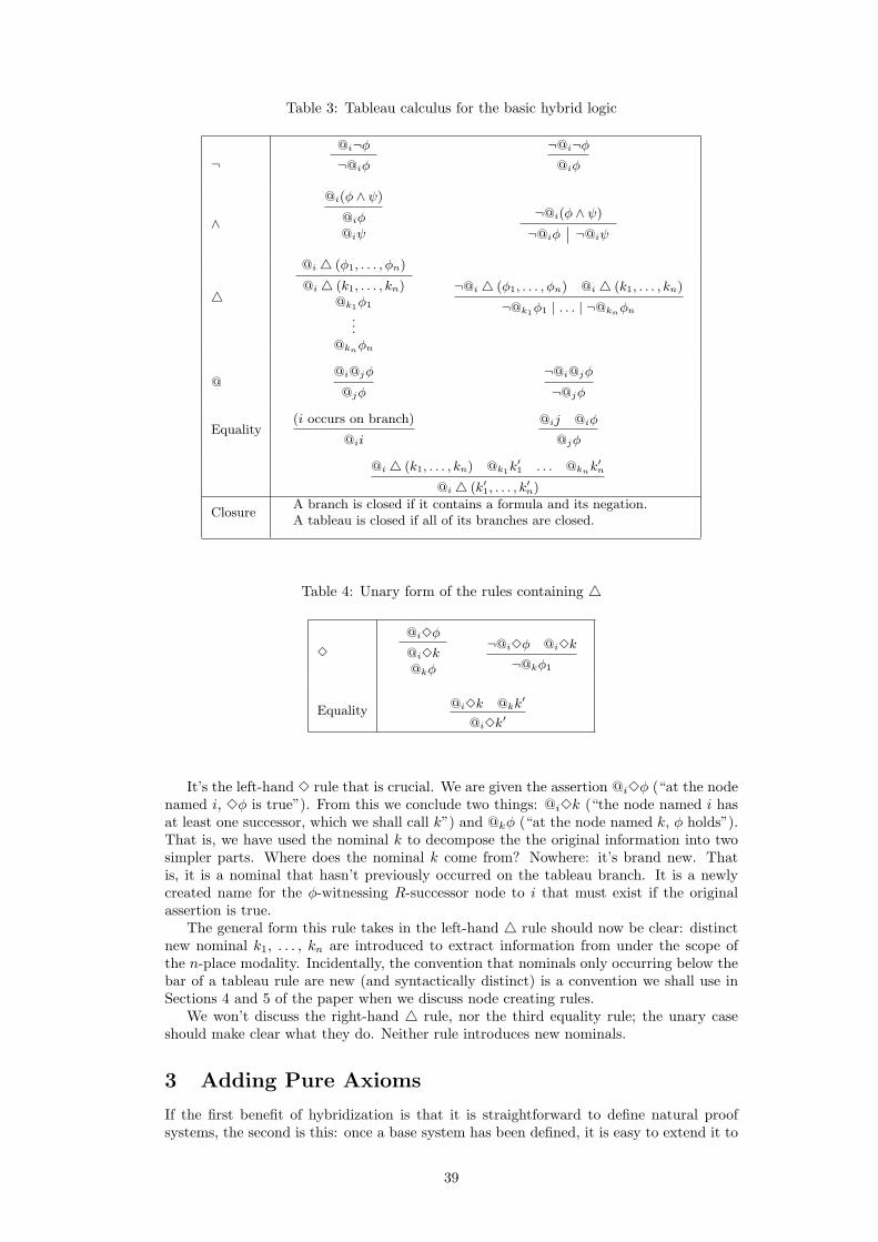
Table 3: Tableau calculus for the basic hybrid logic

¬@i¬φ¬@iφ

¬@i¬φ@iφ

∧

@i(φ ∧ ψ)

@iφ@iψ

¬@i(φ ∧ ψ)

¬@iφ ¬@iψ

4

@i 4 (φ1, . . . , φn)

@i 4 (k1, . . . , kn)@k1φ1

...@knφn

¬@i 4 (φ1, . . . , φn) @i 4 (k1, . . . , kn)

¬@k1φ1 | . . . | ¬@knφn

@@i@jφ

@jφ

¬@i@jφ

¬@jφ

Equality(i occurs on branch)

@ii

@ij @iφ

@jφ

@i 4 (k1, . . . , kn) @k1k′1 . . . @knk

′n

@i 4 (k′1, . . . , k′n)

ClosureA branch is closed if it contains a formula and its negation.A tableau is closed if all of its branches are closed.

Table 4: Unary form of the rules containing 4

3

@i3φ

@i3k@kφ

¬@i3φ @i3k

¬@kφ1

Equality@i3k @kk

′

@i3k′

It’s the left-hand 3 rule that is crucial. We are given the assertion @i3φ (“at the nodenamed i, 3φ is true”). From this we conclude two things: @i3k (“the node named i hasat least one successor, which we shall call k”) and @kφ (“at the node named k, φ holds”).That is, we have used the nominal k to decompose the the original information into twosimpler parts. Where does the nominal k come from? Nowhere: it’s brand new. Thatis, it is a nominal that hasn’t previously occurred on the tableau branch. It is a newlycreated name for the φ-witnessing R-successor node to i that must exist if the originalassertion is true.

The general form this rule takes in the left-hand 4 rule should now be clear: distinctnew nominal k1, . . . , kn are introduced to extract information from under the scope ofthe n-place modality. Incidentally, the convention that nominals only occurring below thebar of a tableau rule are new (and syntactically distinct) is a convention we shall use inSections 4 and 5 of the paper when we discuss node creating rules.

We won’t discuss the right-hand 4 rule, nor the third equality rule; the unary caseshould make clear what they do. Neither rule introduces new nominals.

3 Adding Pure Axioms

If the first benefit of hybridization is that it is straightforward to define natural proofsystems, the second is this: once a base system has been defined, it is easy to extend it to

39

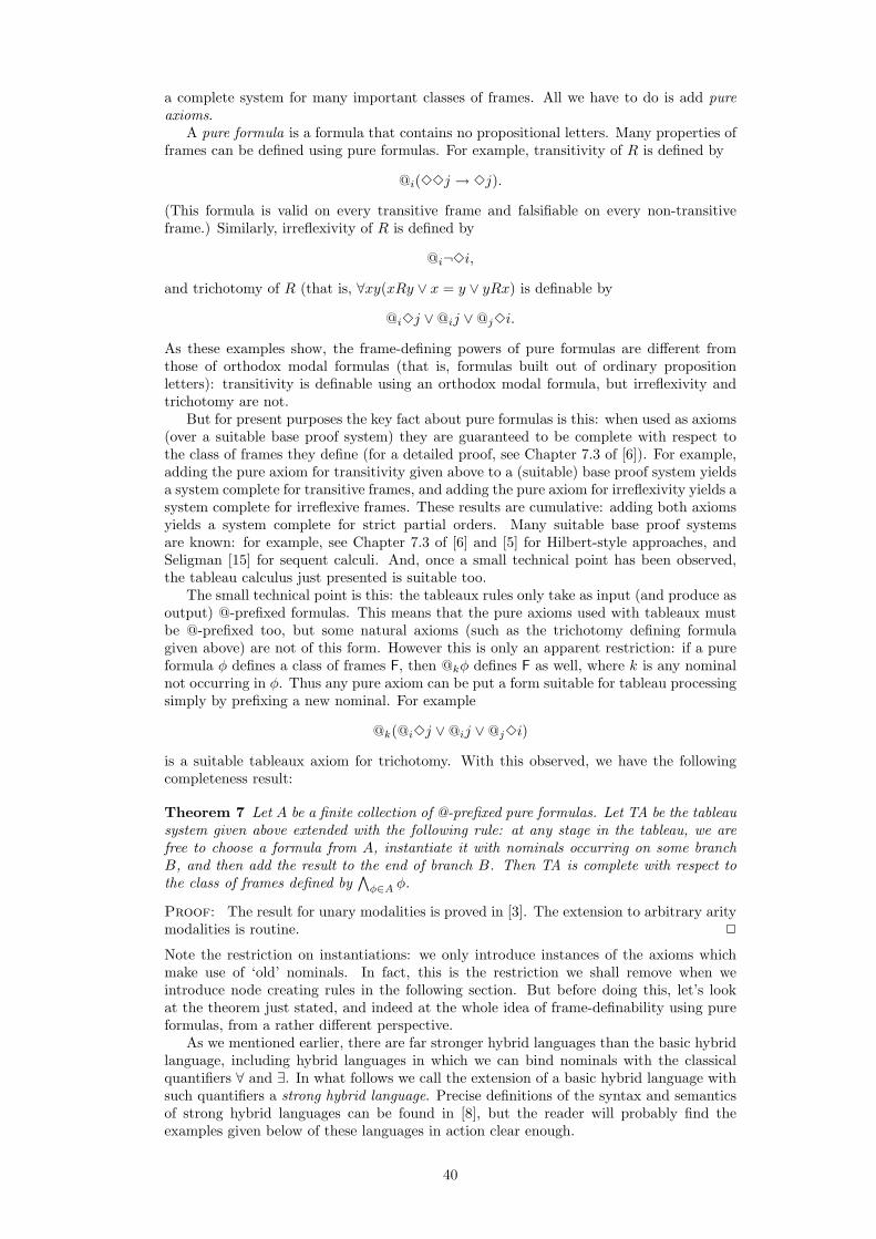
a complete system for many important classes of frames. All we have to do is add pureaxioms.

A pure formula is a formula that contains no propositional letters. Many properties offrames can be defined using pure formulas. For example, transitivity of R is defined by

@i(33j → 3j).

(This formula is valid on every transitive frame and falsifiable on every non-transitiveframe.) Similarly, irreflexivity of R is defined by

@i¬3i,

and trichotomy of R (that is, ∀xy(xRy ∨ x = y ∨ yRx) is definable by

@i3j ∨@ij ∨@j3i.

As these examples show, the frame-defining powers of pure formulas are different fromthose of orthodox modal formulas (that is, formulas built out of ordinary propositionletters): transitivity is definable using an orthodox modal formula, but irreflexivity andtrichotomy are not.

But for present purposes the key fact about pure formulas is this: when used as axioms(over a suitable base proof system) they are guaranteed to be complete with respect tothe class of frames they define (for a detailed proof, see Chapter 7.3 of [6]). For example,adding the pure axiom for transitivity given above to a (suitable) base proof system yieldsa system complete for transitive frames, and adding the pure axiom for irreflexivity yields asystem complete for irreflexive frames. These results are cumulative: adding both axiomsyields a system complete for strict partial orders. Many suitable base proof systemsare known: for example, see Chapter 7.3 of [6] and [5] for Hilbert-style approaches, andSeligman [15] for sequent calculi. And, once a small technical point has been observed,the tableau calculus just presented is suitable too.

The small technical point is this: the tableaux rules only take as input (and produce asoutput) @-prefixed formulas. This means that the pure axioms used with tableaux mustbe @-prefixed too, but some natural axioms (such as the trichotomy defining formulagiven above) are not of this form. However this is only an apparent restriction: if a pureformula φ defines a class of frames F, then @kφ defines F as well, where k is any nominalnot occurring in φ. Thus any pure axiom can be put a form suitable for tableau processingsimply by prefixing a new nominal. For example

@k(@i3j ∨@ij ∨@j3i)

is a suitable tableaux axiom for trichotomy. With this observed, we have the followingcompleteness result:

Theorem 7 Let A be a finite collection of @-prefixed pure formulas. Let TA be the tableausystem given above extended with the following rule: at any stage in the tableau, we arefree to choose a formula from A, instantiate it with nominals occurring on some branchB, and then add the result to the end of branch B. Then TA is complete with respect tothe class of frames defined by

∧φ∈A φ.

Proof: The result for unary modalities is proved in [3]. The extension to arbitrary aritymodalities is routine. 2

Note the restriction on instantiations: we only introduce instances of the axioms whichmake use of ‘old’ nominals. In fact, this is the restriction we shall remove when weintroduce node creating rules in the following section. But before doing this, let’s lookat the theorem just stated, and indeed at the whole idea of frame-definability using pureformulas, from a rather different perspective.

As we mentioned earlier, there are far stronger hybrid languages than the basic hybridlanguage, including hybrid languages in which we can bind nominals with the classicalquantifiers ∀ and ∃. In what follows we call the extension of a basic hybrid language withsuch quantifiers a strong hybrid language. Precise definitions of the syntax and semanticsof strong hybrid languages can be found in [8], but the reader will probably find theexamples given below of these languages in action clear enough.

40

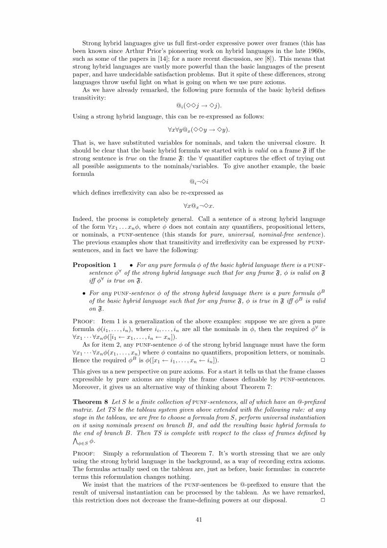
Strong hybrid languages give us full first-order expressive power over frames (this hasbeen known since Arthur Prior’s pioneering work on hybrid languages in the late 1960s,such as some of the papers in [14]; for a more recent discussion, see [8]). This means thatstrong hybrid languages are vastly more powerful than the basic languages of the presentpaper, and have undecidable satisfaction problems. But it spite of these differences, stronglanguages throw useful light on what is going on when we use pure axioms.

As we have already remarked, the following pure formula of the basic hybrid definestransitivity:

@i(33j → 3j).

Using a strong hybrid language, this can be re-expressed as follows:

∀x∀y@x(33y → 3y).

That is, we have substituted variables for nominals, and taken the universal closure. Itshould be clear that the basic hybrid formula we started with is valid on a frame F iff thestrong sentence is true on the frame F: the ∀ quantifier captures the effect of trying outall possible assignments to the nominals/variables. To give another example, the basicformula

@i¬3i

which defines irreflexivity can also be re-expressed as

∀x@x¬3x.

Indeed, the process is completely general. Call a sentence of a strong hybrid languageof the form ∀x1 . . . xnφ, where φ does not contain any quantifiers, propositional letters,or nominals, a punf-sentence (this stands for pure, universal, nominal-free sentence).The previous examples show that transitivity and irreflexivity can be expressed by punf-sentences, and in fact we have the following:

Proposition 1 • For any pure formula φ of the basic hybrid language there is a punf-sentence φ∀ of the strong hybrid language such that for any frame F, φ is valid on Fiff φ∀ is true on F.

• For any punf-sentence φ of the strong hybrid language there is a pure formula φB

of the basic hybrid language such that for any frame F, φ is true in F iff φB is validon F.

Proof: Item 1 is a generalization of the above examples: suppose we are given a pureformula φ(i1, . . . , in), where ii, . . . , in are all the nominals in φ, then the required φ∀ is∀x1 · · · ∀xnφ([i1 ← x1, . . . , in ← xn]).

As for item 2, any punf-sentence φ of the strong hybrid language must have the form∀x1 · · · ∀xnφ(x1, . . . , xn) where φ contains no quantifiers, proposition letters, or nominals.Hence the required φB is φ([x1 ← i1, . . . , xn ← in]). 2

This gives us a new perspective on pure axioms. For a start it tells us that the frame classesexpressible by pure axioms are simply the frame classes definable by punf-sentences.Moreover, it gives us an alternative way of thinking about Theorem 7:

Theorem 8 Let S be a finite collection of punf-sentences, all of which have an @-prefixedmatrix. Let TS be the tableau system given above extended with the following rule: at anystage in the tableau, we are free to choose a formula from S, perform universal instantiationon it using nominals present on branch B, and add the resulting basic hybrid formula tothe end of branch B. Then TS is complete with respect to the class of frames defined by∧

φ∈S φ.

Proof: Simply a reformulation of Theorem 7. It’s worth stressing that we are onlyusing the strong hybrid language in the background, as a way of recording extra axioms.The formulas actually used on the tableau are, just as before, basic formulas: in concreteterms this reformulation changes nothing.

We insist that the matrices of the punf-sentences be @-prefixed to ensure that theresult of universal instantiation can be processed by the tableau. As we have remarked,this restriction does not decrease the frame-defining powers at our disposal. 2

41

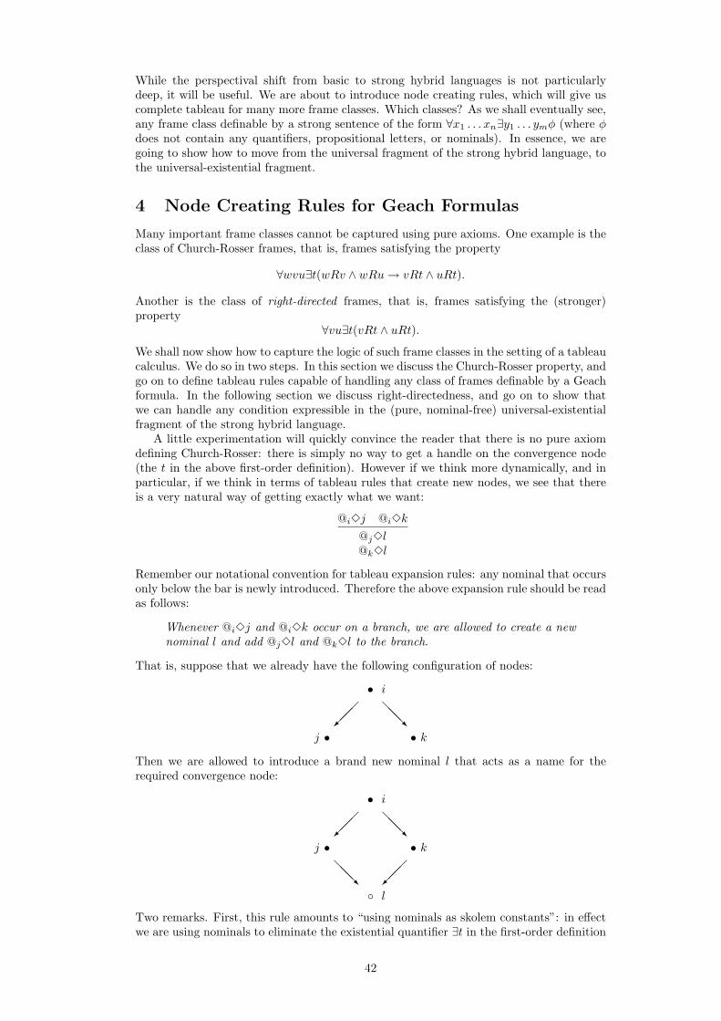
While the perspectival shift from basic to strong hybrid languages is not particularlydeep, it will be useful. We are about to introduce node creating rules, which will give uscomplete tableau for many more frame classes. Which classes? As we shall eventually see,any frame class definable by a strong sentence of the form ∀x1 . . . xn∃y1 . . . ymφ (where φdoes not contain any quantifiers, propositional letters, or nominals). In essence, we aregoing to show how to move from the universal fragment of the strong hybrid language, tothe universal-existential fragment.

4 Node Creating Rules for Geach Formulas

Many important frame classes cannot be captured using pure axioms. One example is theclass of Church-Rosser frames, that is, frames satisfying the property

∀wvu∃t(wRv ∧ wRu→ vRt ∧ uRt).

Another is the class of right-directed frames, that is, frames satisfying the (stronger)property

∀vu∃t(vRt ∧ uRt).

We shall now show how to capture the logic of such frame classes in the setting of a tableaucalculus. We do so in two steps. In this section we discuss the Church-Rosser property, andgo on to define tableau rules capable of handling any class of frames definable by a Geachformula. In the following section we discuss right-directedness, and go on to show thatwe can handle any condition expressible in the (pure, nominal-free) universal-existentialfragment of the strong hybrid language.

A little experimentation will quickly convince the reader that there is no pure axiomdefining Church-Rosser: there is simply no way to get a handle on the convergence node(the t in the above first-order definition). However if we think more dynamically, and inparticular, if we think in terms of tableau rules that create new nodes, we see that thereis a very natural way of getting exactly what we want:

@i3j @i3k

@j3l@k3l

Remember our notational convention for tableau expansion rules: any nominal that occursonly below the bar is newly introduced. Therefore the above expansion rule should be readas follows:

Whenever @i3j and @i3k occur on a branch, we are allowed to create a newnominal l and add @j3l and @k3l to the branch.

That is, suppose that we already have the following configuration of nodes:

• i

��� @@

@Rj • • k

Then we are allowed to introduce a brand new nominal l that acts as a name for therequired convergence node:

• i

��� @

@@Rj • • k

@@@R �

��

◦ l

Two remarks. First, this rule amounts to “using nominals as skolem constants”: in effectwe are using nominals to eliminate the existential quantifier ∃t in the first-order definition

42

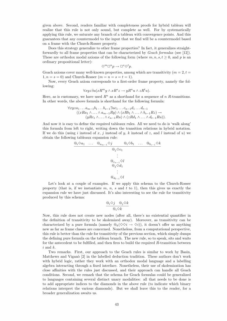
given above. Second, readers familiar with completeness proofs for hybrid tableau willrealize that this rule is not only sound, but complete as well. For by systematicallyapplying this rule, we saturate any branch of a tableau with convergence points. And thisguarantees that any countermodel to the input that we find will be a countermodel basedon a frame with the Church-Rosser property.

Does this strategy generalize to other frame properties? In fact, it generalizes straight-forwardly to all frame properties that can be characterized by Geach formulas (see [12]).These are orthodox modal axioms of the following form (where m,n, s, t ≥ 0, and p is anordinary propositional letter):

3m2np→ 2s3tp.

Geach axioms cover many well-known properties, among which are transitivity (m = 2, t =1, n = s = 0) and Church-Rosser (m = n = s = t = 1).

Now, every Geach axiom corresponds to a first-order frame property, namely the fol-lowing:

∀xyz∃u(xRmy ∧ xRsz → yRnu ∧ zRtu).

Here, as is customary, we have used Rn as a shorthand for a sequence of n R-transitions.In other words, the above formula is shorthand for the following formula:

∀xyza1 . . . am−1b1 . . . bs−1∃uc1 . . . cn−1d1 . . . dt−1

((xRa1 ∧ . . . ∧ am−1Ry) ∧ (xRb1 ∧ . . . ∧ bs−1Rz)→(yRc1 ∧ . . . ∧ cn−1Ru) ∧ (zRd1 ∧ . . . ∧ dt−1Ru)).

And now it is easy to define the required tableaux rules. All we need to do is ‘walk along’this formula from left to right, writing down the transition relations in hybrid notation.If we do this (using i instead of x, j instead of y, k instead of z, and l instead of u) weobtain the following tableaux expansion rule:

@i3a1 . . . @am−13j @i3b1 . . . @bs−13k

@j3c1...

@cn−13l@j3d1

...@dt−13l

Let’s look at a couple of examples. If we apply this schema to the Church-Rosserproperty (that is, if we instantiate m, n, s and t to 1), then this gives us exactly theexpansion rule we have just discussed. It’s also interesting to see the rule for transitivityproduced by this schema:

@i3j @j3k

@i3k

Now, this rule does not create new nodes (after all, there’s no existential quantifier inthe definition of transitivity to be skolemized away). Moreover, as transitivity can becharacterized by a pure formula (namely @k(33i → 3i)), it doesn’t offer us anythingnew as far as frame classes are concerned. Nonetheless, from a computational perspective,this rule is better than the rule for transitivity of the previous section, which simply dumpsthe defining pure formula on the tableau branch. The new rule, so to speak, sits and waitsfor the antecedent to be fulfilled, and then fires to build the required R-transition betweeni and k.

Two remarks. First, our approach to the Geach rules is similar to work by Basin,Matthews and Vigano [2] in the labelled deduction tradition. These authors don’t workwith hybrid logic, rather they work with an orthodox modal language and a labellingalgebra interacting through a fixed interface. Nonetheless, their use of skolemization hasclose affinities with the rules just discussed, and their approach can handle all Geachconditions. Second, we remark that the schema for Geach formulas could be generalizedto languages containing several distinct unary modalities: all that needs to be done isto add appropriate indices to the diamonds in the above rule (to indicate which binaryrelations interpret the various diamonds). But we shall leave this to the reader, for abroader generalization awaits us.

43

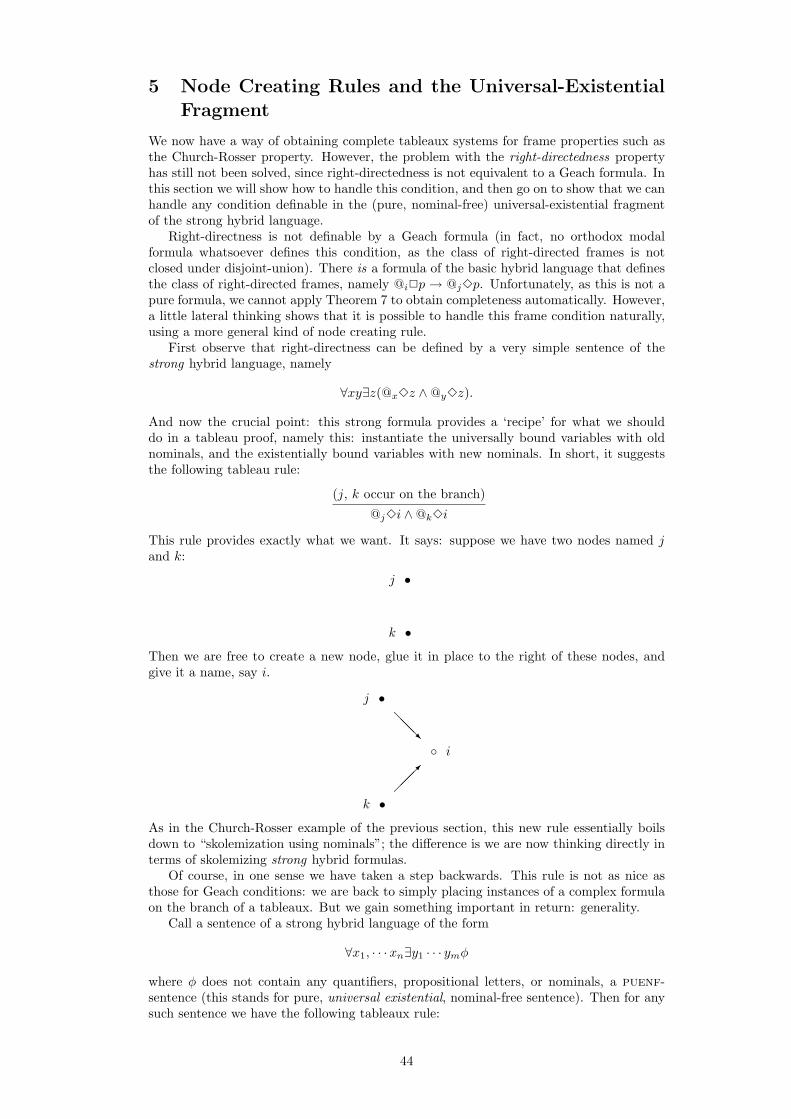
5 Node Creating Rules and the Universal-ExistentialFragment

We now have a way of obtaining complete tableaux systems for frame properties such asthe Church-Rosser property. However, the problem with the right-directedness propertyhas still not been solved, since right-directedness is not equivalent to a Geach formula. Inthis section we will show how to handle this condition, and then go on to show that we canhandle any condition definable in the (pure, nominal-free) universal-existential fragmentof the strong hybrid language.

Right-directness is not definable by a Geach formula (in fact, no orthodox modalformula whatsoever defines this condition, as the class of right-directed frames is notclosed under disjoint-union). There is a formula of the basic hybrid language that definesthe class of right-directed frames, namely @i2p → @j3p. Unfortunately, as this is not apure formula, we cannot apply Theorem 7 to obtain completeness automatically. However,a little lateral thinking shows that it is possible to handle this frame condition naturally,using a more general kind of node creating rule.

First observe that right-directness can be defined by a very simple sentence of thestrong hybrid language, namely

∀xy∃z(@x3z ∧@y3z).

And now the crucial point: this strong formula provides a ‘recipe’ for what we shoulddo in a tableau proof, namely this: instantiate the universally bound variables with oldnominals, and the existentially bound variables with new nominals. In short, it suggeststhe following tableau rule:

(j, k occur on the branch)

@j3i ∧@k3i

This rule provides exactly what we want. It says: suppose we have two nodes named jand k:

j •

k •

Then we are free to create a new node, glue it in place to the right of these nodes, andgive it a name, say i.

j •

@@@R

◦ i

����

k •

As in the Church-Rosser example of the previous section, this new rule essentially boilsdown to “skolemization using nominals”; the difference is we are now thinking directly interms of skolemizing strong hybrid formulas.

Of course, in one sense we have taken a step backwards. This rule is not as nice asthose for Geach conditions: we are back to simply placing instances of a complex formulaon the branch of a tableaux. But we gain something important in return: generality.

Call a sentence of a strong hybrid language of the form

∀x1, · · ·xn∃y1 · · · ymφ

where φ does not contain any quantifiers, propositional letters, or nominals, a puenf-sentence (this stands for pure, universal existential, nominal-free sentence). Then for anysuch sentence we have the following tableaux rule:

44

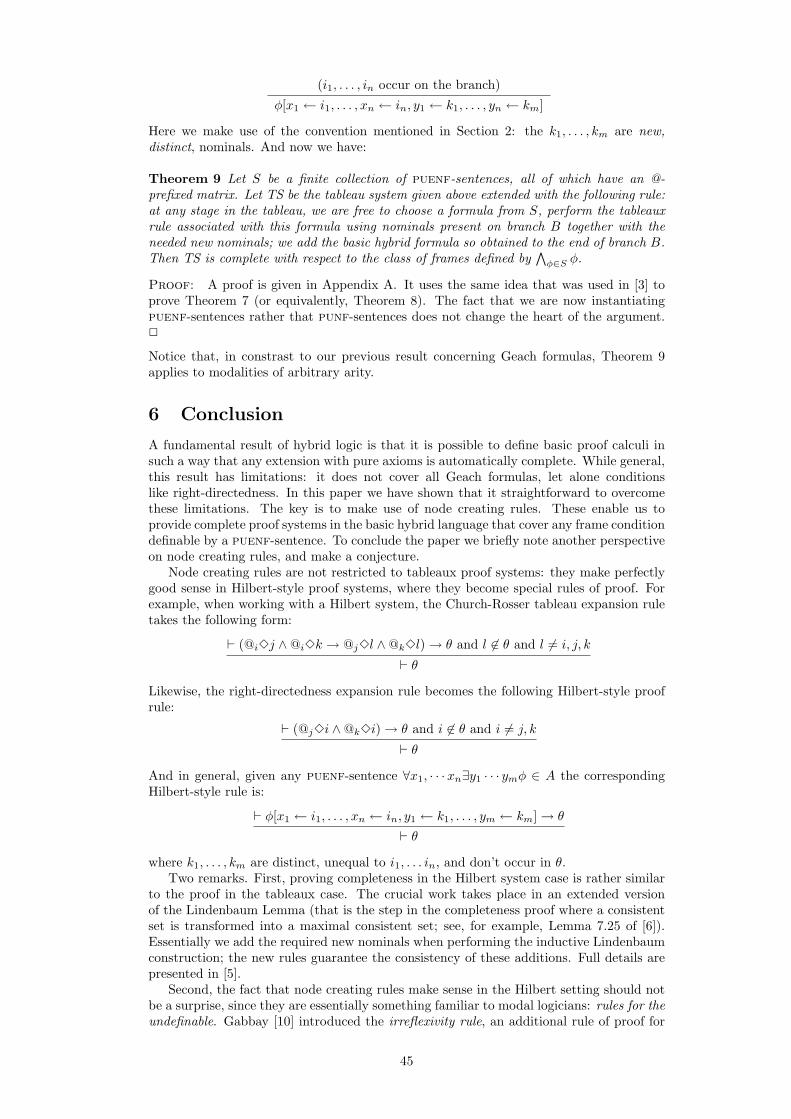
(i1, . . . , in occur on the branch)

φ[x1 ← i1, . . . , xn ← in, y1 ← k1, . . . , yn ← km]

Here we make use of the convention mentioned in Section 2: the k1, . . . , km are new,distinct, nominals. And now we have:

Theorem 9 Let S be a finite collection of puenf-sentences, all of which have an @-prefixed matrix. Let TS be the tableau system given above extended with the following rule:at any stage in the tableau, we are free to choose a formula from S, perform the tableauxrule associated with this formula using nominals present on branch B together with theneeded new nominals; we add the basic hybrid formula so obtained to the end of branch B.Then TS is complete with respect to the class of frames defined by

∧φ∈S φ.

Proof: A proof is given in Appendix A. It uses the same idea that was used in [3] toprove Theorem 7 (or equivalently, Theorem 8). The fact that we are now instantiatingpuenf-sentences rather that punf-sentences does not change the heart of the argument.2

Notice that, in constrast to our previous result concerning Geach formulas, Theorem 9applies to modalities of arbitrary arity.

6 Conclusion

A fundamental result of hybrid logic is that it is possible to define basic proof calculi insuch a way that any extension with pure axioms is automatically complete. While general,this result has limitations: it does not cover all Geach formulas, let alone conditionslike right-directedness. In this paper we have shown that it straightforward to overcomethese limitations. The key is to make use of node creating rules. These enable us toprovide complete proof systems in the basic hybrid language that cover any frame conditiondefinable by a puenf-sentence. To conclude the paper we briefly note another perspectiveon node creating rules, and make a conjecture.

Node creating rules are not restricted to tableaux proof systems: they make perfectlygood sense in Hilbert-style proof systems, where they become special rules of proof. Forexample, when working with a Hilbert system, the Church-Rosser tableau expansion ruletakes the following form:

` (@i3j ∧@i3k → @j3l ∧@k3l)→ θ and l 6∈ θ and l 6= i, j, k

` θ

Likewise, the right-directedness expansion rule becomes the following Hilbert-style proofrule:

` (@j3i ∧@k3i)→ θ and i 6∈ θ and i 6= j, k

` θ

And in general, given any puenf-sentence ∀x1, · · ·xn∃y1 · · · ymφ ∈ A the correspondingHilbert-style rule is:

` φ[x1 ← i1, . . . , xn ← in, y1 ← k1, . . . , ym ← km]→ θ

` θ

where k1, . . . , km are distinct, unequal to i1, . . . in, and don’t occur in θ.Two remarks. First, proving completeness in the Hilbert system case is rather similar

to the proof in the tableaux case. The crucial work takes place in an extended versionof the Lindenbaum Lemma (that is the step in the completeness proof where a consistentset is transformed into a maximal consistent set; see, for example, Lemma 7.25 of [6]).Essentially we add the required new nominals when performing the inductive Lindenbaumconstruction; the new rules guarantee the consistency of these additions. Full details arepresented in [5].

Second, the fact that node creating rules make sense in the Hilbert setting should notbe a surprise, since they are essentially something familiar to modal logicians: rules for theundefinable. Gabbay [10] introduced the irreflexivity rule, an additional rule of proof for

45

orthodox modal language that makes it possible to directly construct irreflexive models,and Venema [16] presents a far-reaching generalization to logics containing the differenceoperator. This is not the place to make detailed comparisons, but we make two remarks.First, because the notion of reference to nodes is primitive in hybrid logic, the hybrid rulesare arguably more natural (though this is partly a matter of taste). Second, in the hybridlogical case, there is a particularly simple answer to the question “But where do such rulescome from?”: they reflect the skolemization possibilities offered by puenf-formulas.

We close with a conjecture. In one sense, we know how many frame classes are cov-ered by this result, namely precisely the frame classes definable by puenf-formulas. Butobviously it would be nice to back this up with a characterization in terms of traditionalcorrespondence theory. We have such a result: in [4] we show that the frame condi-tions by puenf-formulas are exactly the universal-existential closures of strongly boundedfirst-order formulas. This is a large class of formulas, and we conjecture it covers everySahlqvist-definable frame class. If this could be proved it would nicely supplement theresult of Goranko and Vakarelov [11], which states that in reversive hybrid languages (thatis, languages where the set of modalities is closed under converses) every Sahlqvist for-mula is equivalent to a pure formula. Incidentally, note that the sets of puenf-definableand Sahlqvist-definable frame conditions cannot be identical, since many puenf-definable(indeed punf-definable) conditions such as irreflexivity, antisymmetry, and discretenessare not definable by any orthodox modal formula at all.

References

[1] C. Areces, P. Blackburn, and M. Marx. A roadmap on the complexity of hybrid logics. InJ. Flum and M. Rodrıguez-Artalejo, editors, Computer Science Logic, number 1683 in LNCS,pages 307–321. Springer, 1999. Proceedings of the 8th Annual Conference of the EACSL,Madrid, September 1999.

[2] David Basin, Sean Matthews, and Luca Vigano. Labelled propositional modal logics: Theoryand practice. Journal of Logic and Computation, 7(6):685–717, 1997.

[3] P. Blackburn. Internalizing labelled deduction. Journal of Logic and Computation, 10:137–168, 2000.

[4] P. Blackburn and B. ten Cate. Correspondence theory for hybrid logic, 2002. Manuscript,INRIA Lorraine and ILLC, University of Amsterdam.

[5] P. Blackburn and B. ten Cate. Hybrid axiomatics: the propositional case, 2002. Manuscript,INRIA Lorraine and ILLC, University of Amsterdam.

[6] P. Blackburn, M. de Rijke, and Y. Venema. Modal Logic. Cambridge University Press, 2001.

[7] P. Blackburn and M. Marx. Tableaux for quantified hybrid logic. In C. Areces and M. de Ri-jke, editors, Methods for Modalities 2, Workshop Proceedings, November 29-30, 2001. ILLCAmsterdam, 2001.

[8] P. Blackburn and J. Seligman. Hybrid languages. Journal of Logic, Language and Informa-tion, 4(3):251–272, 1995. Special issue on decompositions of first-order logic.

[9] R. Bull. An approach to tense logic. Theoria, 36:282–300, 1970.

[10] D.M. Gabbay. An irreflexivity lemma with applications to axiomatizations of conditions onlinear frames. In U. Monnich, editor, Aspects of Philosophical Logic, pages 67–89. Reidel,Dordrecht, 1981.

[11] Valentin Goranko and Dmiter Vakarelov. Sahlqvist formulas in hybrid polyadic modal logics.Journal of Logic and Computation, 11(5):737–754, 2001. Special issue on hybrid logic.

[12] G. Hughes and M.J. Cresswell. A New Introduction to Modal Logic. Routledge, 1996.

[13] S. Passy and T. Tinchev. An essay in combinatory dynamic logic. Information and Compu-tation, 93:263–332, 1991.

[14] A.N. Prior. Papers on Time and Tense. University of Oxford Press, 1968.

[15] J. Seligman. Internalization: The case of hybrid logics. Journal of Logic and Computation,11(5):671–689, 2001. Special issue on hybrid logic.

[16] Y. Venema. Derivation rules as anti-axioms in modal logic. Journal of Symbolic Logic,58:1003–1034, 1993.

46

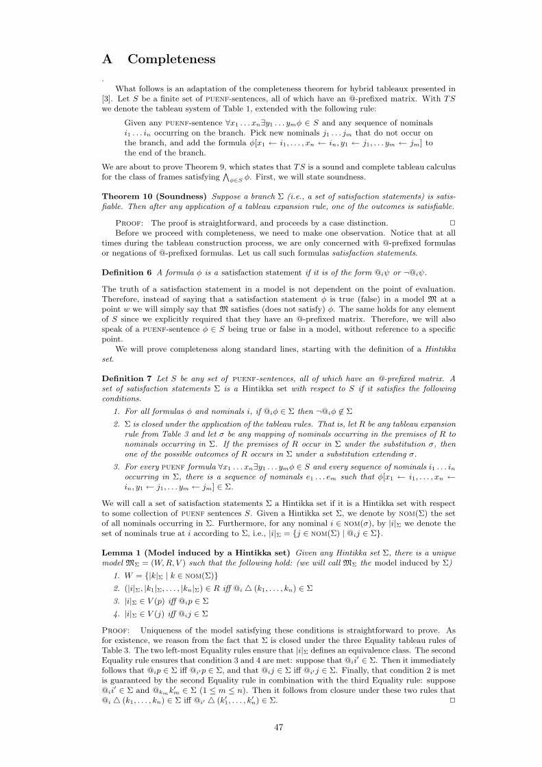
A Completeness

.What follows is an adaptation of the completeness theorem for hybrid tableaux presented in

[3]. Let S be a finite set of puenf-sentences, all of which have an @-prefixed matrix. With TSwe denote the tableau system of Table 1, extended with the following rule:

Given any puenf-sentence ∀x1 . . . xn∃y1 . . . ymφ ∈ S and any sequence of nominalsi1 . . . in occurring on the branch. Pick new nominals j1 . . . jm that do not occur onthe branch, and add the formula φ[x1 ← i1, . . . , xn ← in, y1 ← j1, . . . ym ← jm] tothe end of the branch.

We are about to prove Theorem 9, which states that TS is a sound and complete tableau calculusfor the class of frames satisfying

∧φ∈S φ. First, we will state soundness.

Theorem 10 (Soundness) Suppose a branch Σ (i.e., a set of satisfaction statements) is satis-fiable. Then after any application of a tableau expansion rule, one of the outcomes is satisfiable.

Proof: The proof is straightforward, and proceeds by a case distinction. 2

Before we proceed with completeness, we need to make one observation. Notice that at alltimes during the tableau construction process, we are only concerned with @-prefixed formulasor negations of @-prefixed formulas. Let us call such formulas satisfaction statements.

Definition 6 A formula φ is a satisfaction statement if it is of the form @iψ or ¬@iψ.

The truth of a satisfaction statement in a model is not dependent on the point of evaluation.Therefore, instead of saying that a satisfaction statement φ is true (false) in a model M at apoint w we will simply say that M satisfies (does not satisfy) φ. The same holds for any elementof S since we explicitly required that they have an @-prefixed matrix. Therefore, we will alsospeak of a puenf-sentence φ ∈ S being true or false in a model, without reference to a specificpoint.

We will prove completeness along standard lines, starting with the definition of a Hintikkaset.

Definition 7 Let S be any set of puenf-sentences, all of which have an @-prefixed matrix. Aset of satisfaction statements Σ is a Hintikka set with respect to S if it satisfies the followingconditions.

1. For all formulas φ and nominals i, if @iφ ∈ Σ then ¬@iφ 6∈ Σ

2. Σ is closed under the application of the tableau rules. That is, let R be any tableau expansionrule from Table 3 and let σ be any mapping of nominals occurring in the premises of R tonominals occurring in Σ. If the premises of R occur in Σ under the substitution σ, thenone of the possible outcomes of R occurs in Σ under a substitution extending σ.

3. For every puenf formula ∀x1 . . . xn∃y1 . . . ymφ ∈ S and every sequence of nominals i1 . . . inoccurring in Σ, there is a sequence of nominals e1 . . . em such that φ[x1 ← i1, . . . , xn ←in, y1 ← j1, . . . ym ← jm] ∈ Σ.

We will call a set of satisfaction statements Σ a Hintikka set if it is a Hintikka set with respectto some collection of puenf sentences S. Given a Hintikka set Σ, we denote by nom(Σ) the setof all nominals occurring in Σ. Furthermore, for any nominal i ∈ nom(σ), by |i|Σ we denote theset of nominals true at i according to Σ, i.e., |i|Σ = {j ∈ nom(Σ) | @ij ∈ Σ}.

Lemma 1 (Model induced by a Hintikka set) Given any Hintikka set Σ, there is a uniquemodel MΣ = (W,R, V ) such that the following hold: (we will call MΣ the model induced by Σ)

1. W = {|k|Σ | k ∈ nom(Σ)}2. (|i|Σ, |k1|Σ, . . . , |kn|Σ) ∈ R iff @i 4 (k1, . . . , kn) ∈ Σ

3. |i|Σ ∈ V (p) iff @ip ∈ Σ

4. |i|Σ ∈ V (j) iff @ij ∈ Σ

Proof: Uniqueness of the model satisfying these conditions is straightforward to prove. Asfor existence, we reason from the fact that Σ is closed under the three Equality tableau rules ofTable 3. The two left-most Equality rules ensure that |i|Σ defines an equivalence class. The secondEquality rule ensures that condition 3 and 4 are met: suppose that @ii

′ ∈ Σ. Then it immediatelyfollows that @ip ∈ Σ iff @i′p ∈ Σ, and that @ij ∈ Σ iff @i′j ∈ Σ. Finally, that condition 2 is metis guaranteed by the second Equality rule in combination with the third Equality rule: suppose@ii

′ ∈ Σ and @kmk′m ∈ Σ (1 ≤ m ≤ n). Then it follows from closure under these two rules that

@i 4 (k1, . . . , kn) ∈ Σ iff @i′ 4 (k′1, . . . , k′n) ∈ Σ. 2

47

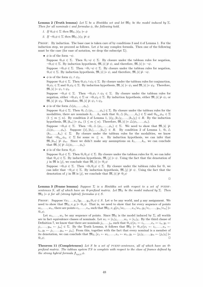
Lemma 2 (Truth lemma) Let Σ be a Hintikka set and let MΣ be the model induced by Σ.Then for all nominals i and formulas φ, the following hold.

1. If @iφ ∈ Σ then MΣ, |i|Σ |= φ

2. If ¬@iφ ∈ Σ then MΣ, |i|Σ 6|= φ

Proof: By induction. The base case is taken care of by conditions 3 and 4 of Lemma 1. For theinduction step, we proceed as follows. Let φ be any complex formula. Then one of the followingmust be the case (for ease of notation, we drop the subscript Σ).

• φ is of the form ¬ψ.

Suppose @iφ ∈ Σ. Then @i¬ψ ∈ Σ. By closure under the tableau rules for negation,¬@iψ ∈ Σ. By induction hypothesis, M, |i| 6|= ψ, and therefore, M, |i| |= ¬ψ.

Suppose ¬@iφ ∈ Σ. Then ¬@i¬ψ ∈ Σ. By closure under the tableau rules for negation,@iψ ∈ Σ. By induction hypothesis, M, |i| |= ψ, and therefore, M, |i| 6|= ¬ψ.

• φ is of the form ψ1 ∧ ψ2.

Suppose @iφ ∈ Σ. Then @iψ1∧ψ2 ∈ Σ. By closure under the tableau rules for conjunction,@iψ1 ∈ Σ and @iψ2 ∈ Σ. By induction hypothesis, M, |i| |= ψ1 and M, |i| |= ψ2. Therefore,M, |i| |= ψ1 ∧ ψ2.

Suppose ¬@iφ ∈ Σ. Then ¬@iψ1 ∧ ψ2 ∈ Σ. By closure under the tableau rules fornegation, either ¬@iψ1 ∈ Σ or ¬@iψ2 ∈ Σ. By induction hypothesis, either M, |i| 6|= ψ1 orM, |i| 6|= ψ2. Therefore, M, |i| 6|= ψ1 ∧ ψ2.

• φ is of the form 4(φ1, . . . , φn).

Suppose @iφ ∈ Σ. Then @i4 (φ1, . . . , φn) ∈ Σ. By closure under the tableau rules for themodalities, there are nominals k1 . . . kn such that @i 4 (k1, . . . , kn) ∈ Σ and @kmφm ∈ Σ(1 ≤ m ≤ n). By condition 2 of Lemma 1, |i|Σ, |k1|Σ, . . . , |kn|Σ) ∈ R. By the inductionhypothesis, M, |km| |= φm (1 ≤ m ≤ n). Therefore, M, |i| |= 4(φ1, . . . , φn).

Suppose ¬@iφ ∈ Σ. Then ¬@i 4 (φ1, . . . , φn) ∈ Σ. We need to show that M, |i| 6|=4(φ1, . . . , φn). Suppose (|i|, |k1|, . . . , |kn|) ∈ R. By condition 2 of Lemma 1, @i 4(k1, . . . , kn) ∈ Σ. By closure under the tableau rules for the modalities, we knowthat ¬@kmφm ∈ Σ for some m ≤ n. By induction hypothesis, we can infer thatM, |km| 6|= φm. Since we didn’t make any assumptions on k1, . . . , kn, we can concludethat M, |i| 6|= 4(φ1, . . . , φn).

• φ is of the form @jψ.

Suppose @iφ ∈ Σ. Then @i@jψ ∈ Σ. By closure under the tableau rules for @, we can inferthat @jψ ∈ Σ. By induction hypothesis, M, |j| |= ψ. Using the fact that the denotation ofj in M is |j|, we conclude that M, |i| |= @jψ

Suppose ¬@iφ ∈ Σ. Then ¬@i@jψ ∈ Σ. By closure under the tableau rules for @, wecan infer that ¬@jψ ∈ Σ. By induction hypothesis, M, |j| 6|= ψ. Using the fact that thedenotation of j in M is |j|, we conclude that M, |i| 6|= @jψ

2

Lemma 3 (Frame lemma) Suppose Σ is a Hintikka set with respect to a set of puenf-sentences S, all of which have an @-prefixed matrix. Let MΣ be the model induced by Σ. ThenMΣ |= φ for all (strong hybrid) formulas φ ∈ S.

Proof: Suppose ∀x1 . . . xn∃y1 . . . ym@zψ ∈ S. Let w be any world, and g any assignment. Weneed to show that MΣ, v, g |= @zφ. That is, we need to show that for every sequence of pointsw1, . . . , wn, there are points v1, . . . , vm such that MΣ, v, g[x1/w1, . . . , xn/wn, y1/v1, . . . , ym/vm] |=@zψ.

Let w1, . . . , wn be any sequence of points. Since MΣ is the model induced by Σ, all worldsare in fact equivalence classes of nominals. Let w1 = |i1|Σ, . . . , wn = |in|Σ. By the third clause ofDefinition 7, we know that there are nominals j1, . . . jm such that @zψ[x1 ← i1, . . . , xn ← in, y1 ←j1, . . . , ym ← jm] ∈ Σ. By the Truth Lemma, it follows that MΣ |= @zψ[x1 ← i1, . . . , xn ←in, y1 ← j1, . . . , ym ← jm]. From this, together with the fact that every nominal is a member ofits denotation, we can conclude that MΣ, [x1 ← w1, . . . , xn ← wn, y1 ← |j1|Σ, . . . , ym ← |jn|Σ] |=@zψ. 2

Theorem 11 (Completeness) Let S be a set of puenf-sentences, all of which have an @-prefixed matrix. The tableau system TS is complete with respect to the class of frames defined bythe strong hybrid formula

∧φ∈S φ.

48

Proof: Given a set of satisfaction statements Σ and a fully developed (possibly infinite)open TS tableau starting with Σ. Since the tableau is open, there must be a fully developedbranch that doesn’t contain an inconsistent pair of formulas. Let Γ be the set of all formulasoccurring on this branch. Γ is a Hintikka set and Σ ⊆ Γ. Let MΓ be the model induced by Γ. Bythe Truth Lemma, MΓ, |i| |= Σ for all nominals i. By the Frame Lemma, MΓ satisfies all stronghybrid formulas of S. Therefore, Σ is satisfiable in a model that satisfies

∧φ∈S φ. 2

49