Lectures 5 & 6 6.263/16.37 Introduction to Queueing Theory

Lectures 5 & 6

6.263/16.37

Introduction to Queueing Theory

Eytan Modiano MIT, LIDS

Eytan Modiano Slide 1

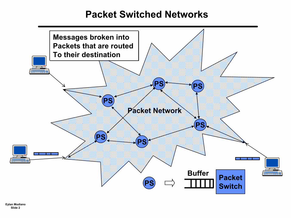
Packet Switched Networks

Packet Network PS

PS PS

PS

PSPS

PS Buffer Packet

Switch

Messages broken into Packets that are routed To their destination

Eytan ModianoSlide 2

Queueing Systems

• Used for analyzing network performance

• In packet networks, events are random – Random packet arrivals – Random packet lengths

• While at the physical layer we were concerned with bit-error-rate, at the network layer we care about delays

– How long does a packet spend waiting in buffers ? – How large are the buffers ?

• In circuit switched networks want to know call blocking probability – How many circuits do we need to limit the blocking probability?


Random events

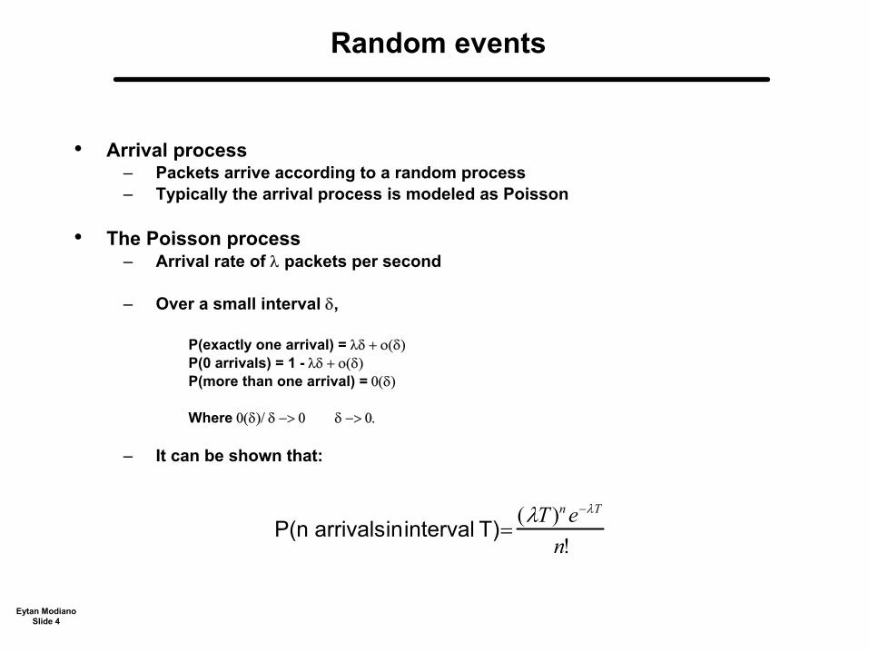
• Arrival process – Packets arrive according to a random process – Typically the arrival process is modeled as Poisson

• The Poisson process – Arrival rate of λ packets per second

– Over a small interval δ,

P(exactly one arrival) = λδ + ο(δ) P(0 arrivals) = 1 - λδ + ο(δ) P(more than one arrival) = 0(δ)

Where 0(δ)/ δ −> 0 �� δ −> 0.

– It can be shown that:

P(n arrivalsininterval T)= ( λT )n e−λT

n!


The Poisson Process

P(n arrivalsininterval T)= ( λT )n e−λT

n!

n = number of arrivals in T

It can be shown that,

E[n] = λT

E[n2] = λT + (λT)2

σ 2 = E[(n -E[n])2] = E[n2] - E[n]2 = λT


Inter-arrival times

• Time that elapses between arrivals (IA)

P(IA <= t) = 1 - P(IA > t) = 1 - P(0 arrivals in time t)

= 1 - e-λt

• This is known as the exponential distribution – Inter-arrival CDF = FIA (t) = 1 - e-λt

– Inter-arrival PDF = d/dt FIA(t) = λe-λt

• The exponential distribution is often used to model the service times (I.e.,the packet length distribution)


Markov property (Memoryless)

P(T ≤ t0 + t | T > t0 ) = P(T ≤ t)

Pr oof :

P(T ≤ t0 + t | T > t0 ) = P(t0 < T ≤ t0 + t) P(T > t0 )

t 0 +t∫ λe−λtdt −e− λt | t0

t0 + t −e−λ ( t +t 0 ) + e−λ ( t0 ) t 0= = = ∞ ∞ e−λ ( t0 )

∫ λe− λtdt −e−λt |t 0 t0

= 1 − e − λt = P(T ≤ t)

• Previous history does not help in predicting the future!

• Distribution of the time until the next arrival is independent of when the last arrival occurred!


Example

• Suppose a train arrives at a station according to a Poisson processwith average inter-arrival time of 20 minutes

• When a customer arrives at the station the average amount of timeuntil the next arrival is 20 minutes

– Regardless of when the previous train arrived

• The average amount of time since the last departure is 20 minutes!

• Paradox: If an average of 20 minutes passed since the last trainarrived and an average of 20 minutes until the next train, then anaverage of 40 minutes will elapse between trains

– But we assumed an average inter-arrival time of 20 minutes! – What happened?


Properties of the Poisson process

• Merging Property λ1 λ2 ∑λi

λk Let A1, A2, … Ak be independent Poisson Processes of rate λ1, λ2, …λk

A = ∑Ai is also Poisson of rate = ∑λi

• Splitting property – Suppose that every arrival is randomly routed with probability P to

stream 1 and (1-P) to stream 2 – Streams 1 and 2 are Poisson of rates Pλ and (1-P)λ respectively

P

1-P

λP λ

λ(1−P) Eytan Modiano

Slide 9

Queueing Models

Customers Queue/buffer

• Model for – Customers waiting in line – Assembly line – Packets in a network (transmission line)

• Want to know – Average number of customers in the system – Average delay experienced by a customer

• Quantities obtained in terms of – Arrival rate of customers (average number of customers per unit time) – Service rate (average number of customers that the server can serve

per unit time)

server


Little’s theorem

Network (system) (N,T)λ packet per second

• N = average number of packets in system • T = average amount of time a packet spends in the system • λ = arrival rate of packets into the system

(not necessarily Poisson)

• Little’s theorem: N = λT – Can be applied to entire system or any part of it – Crowded system -> long delays

On a rainy day people drive slowly and roads are more congested!


Proof of Little’s Theorem

α(t), β(t)

t1 t2 t3 t4

• α(t) = number of arrivals by time t • β(t) = number of departures by time t • ti = arrival time of ith customer • Ti = amount of time ith customer spends in the system • N(t) = number of customers in system at time t = α(t) - β(t)

• Similar proof for non First-come-first-serve

α(t)

T1 T2

T3 T4

β(t)


Proof of Little’s Theorem

t1Nt = ∫ N (τ )dτ = timeave.numberof customersinqueue

t 0

N = Limitt→ ∞ Nt = steadystatetimeave.

λt = α (t) / t, λ = Limitt→ ∞ λt = arrival rate

α

∑( t)

Ti Tt = i= 0

α (t) = timeave.systemdelay, T = Limitt → ∞ Tt

• Assume above limits exists, assume Ergodic systemα ( t)

N (t) = α(t) − β(t ) ⇒ Nt = ∑ i=1 Ti

t α (t ) α( t )

α ( t)N = limt → ∞

∑i =1 Ti , T = limt →∞

∑i =1 Ti ⇒ ∑ i=1

Ti = α (t)T t α (t)

α ( t) α ( t)

Eytan Modiano N = ∑ i=1

Ti = (α(t)) ∑ i=1 Ti = λT

Slide 13 t t α (t)

Application of little’s Theorem

• Little’s Theorem can be applied to almost any system or part of it

• Example: Customers server

Queue/buffer

1) The transmitter: DTP = packet transmission time – Average number of packets at transmitter = λDTP = ρ = link utilization

2) The transmission line: Dp = propagation delay – Average number of packets in flight = λDp

3) The buffer: Dq = average queueing delay – Average number of packets in buffer = Nq = λDq

4) Transmitter + buffer – Average number of packets = ρ + Nq


Application to complex system

λ 1

λ

λ

2

3 λ 1

λ 2

λ 3

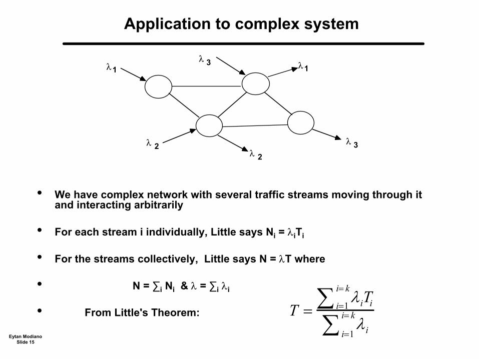
• We have complex network with several traffic streams moving through itand interacting arbitrarily

• For each stream i individually, Little says Ni = λiTi

• For the streams collectively, Little says N = λT where

• N = ∑i Ni & λ = ∑i λi i= k

• From Little's Theorem: T = ∑ i=1 λiTi

i= k

Eytan Modiano ∑ i=1

λi Slide 15

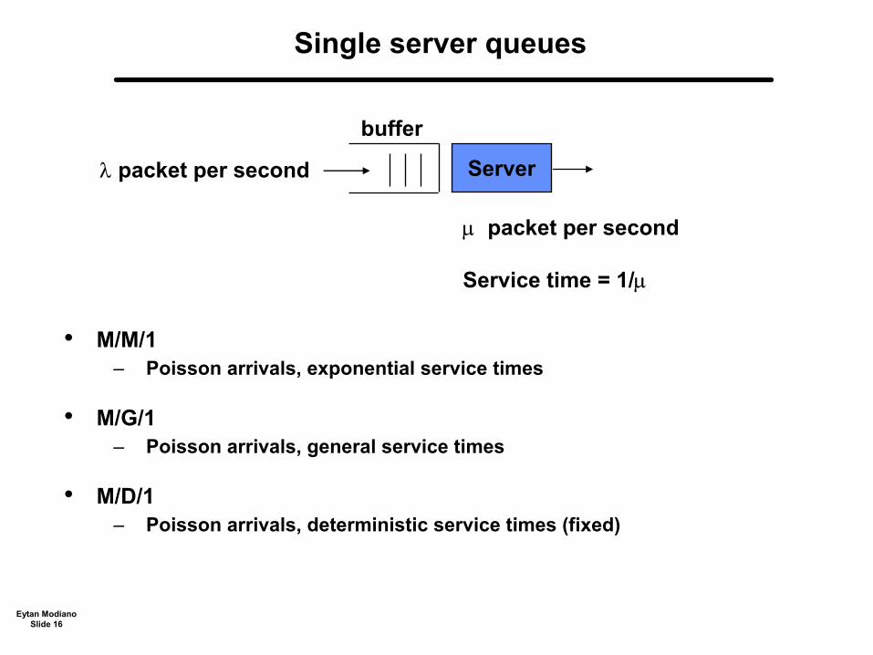
Single server queues

buffer

λ packet per second

• M/M/1

Server

µ packet per second

Service time = 1/µ

– Poisson arrivals, exponential service times

• M/G/1 – Poisson arrivals, general service times

• M/D/1 – Poisson arrivals, deterministic service times (fixed)


Markov Chain for M/M/1 system

λδ λδ λδ λδ

0 1 2

1−λδ

k

µδ µδ µδ µδ

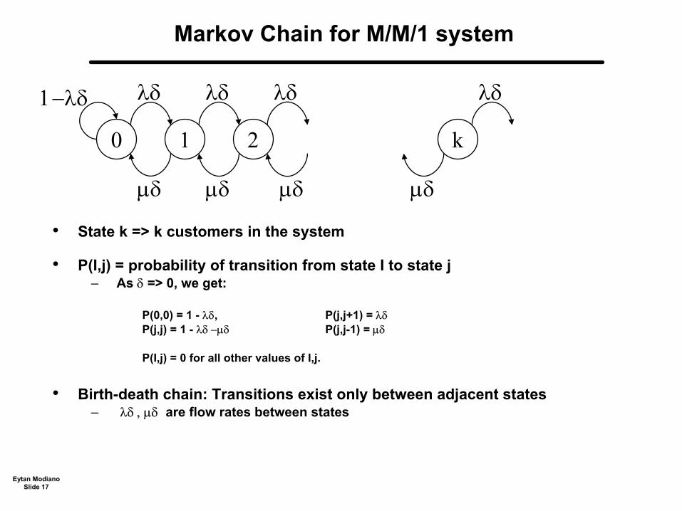
• State k => k customers in the system

• P(I,j) = probability of transition from state I to state j – As δ => 0, we get:

P(0,0) = 1 - λδ, P(j,j+1) = λδ P(j,j) = 1 - λδ −µδ P(j,j-1) = µδ

P(I,j) = 0 for all other values of I,j.

• Birth-death chain: Transitions exist only between adjacent states – λδ , µδ are flow rates between states


Equilibrium analysis

• We want to obtain P(n) = the probability of being in state n

• At equilibrium λP(n) = µP(n+1) for all n – Local balance equations between two states (n, n+1) – P(n+1) = (λ/µ)P(n) = ρP(n), ρ = λ/µ

• It follows: P(n) = ρn P(0) ∑i

∞

= 0 P(n) = 1

• Now by axiom of probability: ∞ P(0)

⇒ ∑i =0 ρnP(0) =

1− ρ= 1

⇒ P(0) = 1 − ρ

P(n) = ρ n(1 − ρ)


Average queue size

∞ ∞

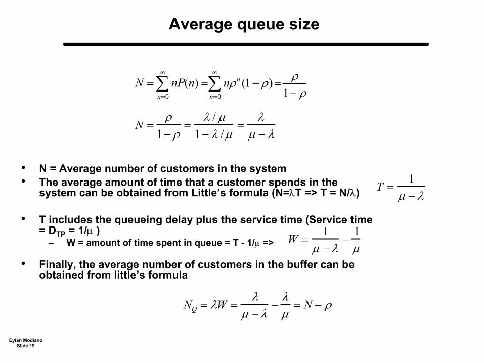
N = ∑ nP(n) =∑ nρn (1 − ρ) = ρ

n=0 n=0 1− ρ

N =ρ

= λ / µ

= λ

1 − ρ 1 − λ / µ µ − λ

• N = Average number of customers in the system • The average amount of time that a customer spends in the T =

1 system can be obtained from Little’s formula (N=λT => T = N/λ) µ − λ

• T includes the queueing delay plus the service time (Service time = DTP = 1/µ ) 1

– W = amount of time spent in queue = T - 1/µ => W = µ − λ

− 1 µ

• Finally, the average number of customers in the buffer can be obtained from little’s formula

λNQ = λW =

µ − λ−

λ= N − ρ

µ


Example (fast food restaurant)

• Customers arrive at a fast food restaurant at a rate of 100 per hourand take 30 seconds to be served.

• How much time do they spend in the restaurant?

– Service rate = µ = 60/0.5=120 customers per hour – T = 1/µ−λ = 1/(120-100) = 1/20 hrs = 3 minutes

• How much time waiting in line? – W = T - 1/µ = 2.5 minutes

• How many customers in the restaurant? – N = λT = 5

• What is the server utilization? – ρ = λ/µ = 5/6


Packet switching vs. Circuit switching

1

λ/M

λ/MN

λ/M 1 2 3 M 1 2 3 M

TDM, Time Division MultiplexingEach user can send µ/N packets/sec and has packet arriving at rate λ/N packets/sec

D = M / µ + M (λ / µ)

M/M/1(µ − λ ) formula

Packets generated at random times

λ/M λ Buffer µ packets/secStatistical Mutliplexer

D = 1/ µ + ( λ / µ) M/M/1

λ/M (µ − λ) formula


2

Circuit (tdm/fdm) vs. Packet switching

Average Packet Service Time (slots)

1

10

100

0 0.2 0.4 0.6 0.8 1

Total traffic load, packets per slot

Aver

age

Serv

ice

Tim

e

TDM with 20 sources

Ideal Statistical Multiplexing (M/D/1)

Eytan ModianoSlide 22

M server systems: M/M/m

buffer

λ packet per second

Server

M servers µ packet per second, per server

• Departure rate is proportional to the number of servers in use

• Similar Markov chain:

λδ λδ λδ

m

λδ

m+1

λδ

0 1 2

1−λδ

µδ 2µδ 3µδ mµδ mµδ

Server


M/M/m queue

λP(n − 1) = nµP(n) n ≤ m • Balance equations:

λP(n − 1) = mµP(n) n > m

P(0)( mρ )n / n! n ≤ m , ρ =

λ≤ 1P(n ) =

P(0)( mmρn ) / m! n > m mµ

• Again, solve for P(0): m −1 (mρ) n ( mρ )m −1

P(0) = ∑ n =0 n!

+ m!(1− ρ)

n= ∞

PQ = ∑ P( n) = P(0)(mρ)m

n= m m!(1 − ρ)

n= ∞ n=∞ m + n ρNQ = ∑ nP(n + m) = ∑nP(0)(

mmρ ) = PQ (1 − ρ

) n=0 n =0 m!

W = N

λ Q , T = W + 1/ µ, N =λT =λ / µ + NQ


Applications of M/M/m

• Bank with m tellers • Network with parallel transmission lines

m lines, each of rate µ Use

λNode

A Node

B M/M/m formula

VS One line of rate mµ Use

λNode

A Node

B M/M/1 formula

• When the system is lightly loaded, PQ~0, and Single server is m times faster • When system is heavily loaded, queueing delay dominates and systems are

roughly the same Eytan Modiano

Slide 25

M/M/Infinity

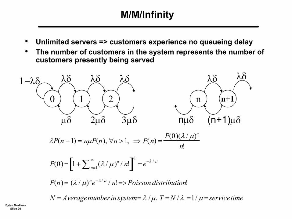
• Unlimited servers => customers experience no queueing delay • The number of customers in the system represents the number of

customers presently being served

λδ λδ λδ

n

λδ

n+1

λδ

0 1 2

1−λδ

µδ 2µδ 3µδ nµδ (n+1)µδ

λP(n − 1) = nµP(n), ∀n > 1, ⇒ P( n) = P(0)(λ / µ)n

n!

∞ −1 P(0) = [1 + ∑ n=1

(λ / µ)n / n!] = e−λ / µ

P(n ) = (λ / µ) ne− λ / µ / n! => Poisson distribution!

N = Averagenumber in system =λ / µ, T = N / λ =1/ µ = servicetime Eytan Modiano

Slide 26

Blocking Probability

• A circuit switched network can be viewed as a Multi-server queueing system

– Calls are blocked when no servers available - “busy signal” – For circuit switched network we are interested in the call blocking

probability

• M/M/m/m system – m servers => m circuits – Last m indicated that the system can hold no more than m users

• Erlang B formula – Gives the probability that a caller finds all circuits busy – Holds for general call arrival distribution (although we prove

Markov case only)

PB = ∑

( m

λ / µ)m / m!

n= 0(λ / µ)n / n!


M/M/m/m system: Erlang B formula

λδ λδ λδ λδ

0 1 2

1−λδ

m

µδ 2µδ 3µδ mµδ

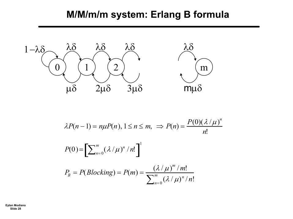
λP(n − 1) = nµP(n ), 1 ≤ n ≤ m, ⇒ P(n) = P(0)( λ / µ)n

n! −1m

P(0) = [∑n= 0(λ / µ)n / n!]

PB = P( Blocking) = P(m) = ( m

λ / µ)m / m!

∑n= 0(λ / µ) n / n!


Erlang B formula

• System load usually expressed in Erlangs – A= λ/µ = (arrival rate)*(ave call duration) = average load PB =

( mA)m / m!

– Formula insensitive to λ and µ but only to their ratio ∑n= 0( A)n / n!

• Used for sizing transmission line – How many circuits does the satellite need to support? – The number of circuits is a function of the blocking probability that we can tolerate

Systems are designed for a given load predictions and blocking probabilities (typically small)

• Example – Arrival rate = 4 calls per minute, average 3 minutes per call => A = 12

– How many circuits do we need to provision? Depends on the blocking probability that we can tolerate

Circuits PB 20 1% 15 8% 7 30%


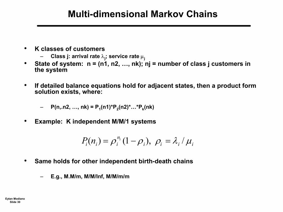
Multi-dimensional Markov Chains

• K classes of customers – Class j: arrival rate λj; service rate µj

• State of system: n = (n1, n2, …, nk); nj = number of class j customers inthe system

• If detailed balance equations hold for adjacent states, then a product formsolution exists, where:

– P(n,.n2, …, nk) = P1(n1)*P2(n2)*…*Pk(nk)

• Example: K independent M/M/1 systems

Pi (ni ) = ρini (1 − ρi ), ρi = λi / µi

• Same holds for other independent birth-death chains

– E.g., M.M/m, M/M/Inf, M/M/m/m


Truncation

• Eliminate some of the states – E.g., for the K M/M/1 queues, eliminate all states where n1+n2+…+nk > K1 (some constant)

• Resulting chain must remain irreducible – All states must communicate

Product form for stationary distribution of the truncated system

• E.g., K independent M/M/1 queues

nK nKP(n1, n2 ,...nk ) =

ρ1 n1ρ2

n2....ρ K , G =∑ ρn1ρ2 n2....ρK1G n∈S

• E.g., K independent M/M/inf queues

P(n1, n2 ,...nk ) = (ρ1

n1 / n1!)(ρ2 n2 / n2!)....(ρK nK / nk !)G

nK / nk !), G =∑(ρ1

n1 / n1!)(ρn2 / n2!)....(ρK2 n∈S

– G is a normalization constant that makes P(n) a distribution – S is the set of states in the truncated system


Example

• Two session classes in a circuit switched system – M channels of equal capacity – Two session types:

Type 1: arrival rate λ1 and service rate µ1 Type 2: arrival rate λ2 and service rate µ2

• System can support up to M sessions of either class – If µ1= µ2, treat system as an M/M/m/m queue with arrival rate λ1+ λ2

– When µ1=! µ2 need to know the number of calls in progress of each session type – Two dimensional markov chain state = (n1, n2) – Want P(n1, n2): n1+n2 <=m

• Can be viewed as truncated M/M/Inf queues – Notice that the transition rates in the M/M/Inf queue are the same as those in a

truncated M/M/m/m queue

i = m j = m −i

P(n1, n2 ) = (ρ1

n1 / n1!)(ρ2 n2 / n2!) , G = ∑ ∑(ρi / i!)(ρ2

j / j!), n1+ n2≤ m1G i =0 j =0

– Notice that the double sum counts only states for which j+i <= m Eytan Modiano

Slide 32

PASTA: Poisson Arrivals See Time Averages

• The state of an M/M/1 queue is the number of customers in the system

• More general queueing systems have a more general state that mayinclude how much service each customer has already received

• For Poisson arrivals, the arrivals in any future increment of time is independent of those in past increments and for many systems of interest, independent of the present state S(t) (true for M/M/1, M/M/m, and M/G/1).

• For such systems, P{S(t)=s|A(t+δ)-A(t)=1} = P{S(t)=s} – (where A(t)= # arrivals since t=0)

• In steady state, arrivals see steady state probabilities


Occupancy distribution upon arrival

• Arrivals may not always see the steady-state averages

• Example: – Deterministic arrivals 1 per second – Deterministic service time of 3/4 seconds

λ = 1 packets/second T = 3/4 seconds (no queueing)

N = λT = Average occupancy = 3/4

• However, notice that an arrival always finds the system empty!


Occupancy upon arrival for a M/M/1 queue

an = Lim t-> inf (P (N(t) = n | an arrival occurred just after time t)) Pn = Lim t-> inf (P(N(t) = n))

For M/M/1 systems an = Pn

Proof: Let A(t, t+δ) be the event that and arrival occurred between t and t+δ

an (t) = Lim t-> inf (P (N(t) = n| A(t, t+δ) ) = Lim t-> inf (P (N(t) = n, A(t, t+δ) )/P(A(t, t+δ) ) = Lim t-> inf P(A(t, t+δ)| N(t) = n)P(N(t) = n)/P(A(t, t+δ) )

• Since future arrivals are independent of the state of the system,

P(A(t, t+δ)| N(t) = n)= P(A(t, t+δ))

• Hence, an (t) = P(N(t) = n) = Pn(t)

• Taking limits as t-> infinity, we obtain an = Pn

• Result holds for M/G/1 systems as well Eytan Modiano

Slide 35

Lectures 5 & 6 6.263/16.37 Introduction to Queueing Theory

Documents

Transcript of Lectures 5 & 6 6.263/16.37 Introduction to Queueing Theory