1

Lecturer notes on DBMS By DILLIP RANJA NAYAK

1. INTRODUCTION

Facts-Statements of things done or things existing. What Is Data? : A sequence of characters stored in computer memory or storage. It is nothing, it is the convey of meaning. Information-organized data Knowledge-information imbued with intelligence. Database: A database is a software system which consists relational data used by various applications. Database Management System: A Database Management System (DBMS) is a software system that facilitates the process defining, constructing, manages, control and modify database.

File Systems: •File is uninterrupted, unstructured collection of information •File operations: delete, catalog, create, rename, open, close, read, write.

File Management System Problems: •Data redundancy •Data Access: New request-new program •Data is not isolated from the access •Concurrent program execution •Difficulties with security •Integrity.

Use of DBMS Data independence and efficient access. Reduced application development time. Data integrity and security. Uniform data administration. Concurrent access, recovery from crashes.

ADVANTAGES OF A DBMS:

Data independence: Application programs should be as independent as possible from details of

data representation and storage.

Data integrity and security: If data is always accessed through the DBMS, the DBMS can

enforce integrity constraints on the data.

Data administration: When several users share the data, centralizing the administration of data

can or significant improvements.

2

Data Independence

Applications insulated from how data is structured and stored.

Logical data independence: Protection from changes in logical structure of data.

Physical data independence: Protection from changes in physical structure of data if the data as

being accessed by only one user at a time.

A schema is a description of a particular collection of data, using a given data model

Design of schema

Physical – view: How data is stored, how it is accessed, how data is modified, is data ordered, how data is allocated to computer memory

Conceptual – view: The conceptual schema (sometimes called the logical schema) describes the stored data in terms of the data model of the DBMS. In a relational DBMS, the conceptual schema describes all relations that are stored in the database

Internal – view: External schemas, which usually are also in terms of the data model of the DBMS, allow data access to be customized (and authorized) at the level of individual users or groups of users.

Data abstraction

Abstraction- is the process by which data and programs are defined with a representation similar in form to its meaning, while hiding away the implementation details.

Data Models a data model is a collection of concepts for describing

Internal schema

Conceptual schema

Shema2 Schema1 Schema3

3

Data and Data relationships. Data semantics. Data constraints.

Database Administrator:

A person who has such central control over the system is called a database administrator (DBA)

The DBA creates the original database schema by executing a set of data definition statements in the DDL.

Define Storage structure and access-method. The DBA carries out changes to the schema and physical organization to reflect the

changing needs of the organization, or to alter the physical organization to improve performance.

Granting of authorization for data access. Integrity

DDL-It defines the conceptual schema and also gives some details about how to implement this schema.

DML-It used to manipulate data just like retrival, insert, deletion and modification.

E-R diagrams

Entity: An entity is a “thing” or “object” in the real world that is distinguishable from all other objects. For example, each person in an enterprise is an entity.

Entity set: An entity set is a set of entities of the same type that share the same properties, or attributes. The set of all persons who are customers at a given bank, for example, can be defined as the entity set customer.

Attributes: are descriptive properties possessed by each member of an entity set. Simple and composite attributes: the attributes are simple if they are not divided into subparts. On the other hand, if it divided into subparts is called as "composite attributes". For example, an attribute name could be structured as a composite attribute consisting of first-name, middle-initial, and last-name. Single-valued and multivalve attributes: For instance, the loan-number attribute for a specific loan entity refers to only one loan number. Such attributes are said to be single valued. There may be instances where an attribute has a set of values for a specific entity. Consider an employee entity set with the attribute phone-number. An employee may have zero, one, or several phone numbers, and different employees may have different numbers of phones. This type of attribute is said to be multivalve.

Derived attribute: The value for this type of attribute can be derived from the values of other related attributes or entities.

4

Relationship Sets: A relationship is an association among several entities. A relationship set is a set of relationships of the same type.

Mapping Cardinalities: Mapping cardinalities, or cardinality ratios, express the number of entities to which another entity can be associated via a relationship set. Mapping cardinalities are most useful in describing binary relationship sets, although they can contribute to the description of relationship sets that involve more than two entity sets.

One to one. An entity in A is associated with at most one entity in B, and an entity in B is associated with at most one entity in A.

One to many. An entity in A is associated with any number (zero or more) of entities in B. An entity in B, however, can be associated with at most one entity in A.

Many to one. An entity in A is associated with at most one entity in B. An entity in B, however, can be associated with any number (zero or more) of entities in A.

Many to many. An entity in A is associated with any number (zero or more) of entities in B, and an entity in B is associated with any number (zero or more) of entities in A.

Keys: A key allows us to identify a set of attributes that suffice to distinguish entities from each other. Keys also help uniquely identify relationships, and thus distinguish relationships from each other.

Super key: A super key is a set of one or more attributes that, taken collectively, allow us to identify uniquely an entity in the entity set. For example, the customer-id attribute of the entity set customer is sufficient to distinguish one customer entity from another. Thus, customer-id is a super key. Similarly, the combination of customer-name and customer-id is a super key for the entity set customer. The customer-name attribute of customer is not a super key, because several people might have the same name.

Candidate key: minimal super keys are called candidate keys.

Primary key: which denotes the unique identity is called as primary key. Primary key to denote a candidate key that is chosen by the database designer as the principal means of identifying entities within an entity set. A key (primary, candidate, and super) is a property of the entity set, rather than of the individual entities.

Weak Entity Sets: An entity set may not have sufficient attributes to form a primary key. Such an entity set is termed a weak entity set. An entity set that has a primary key is termed a strong entity set

5

Example-1

For a weak entity set to be meaningful, it must be associated with another entity set, called the identifying or owner entity set. The relationship associating the weak entity set with the identifying entity set is called the identifying relationship. The participation of the weak entity set in the relationship is called total.

In our example, the identifying entity set for payment is loan, and a relationship loan-payment that associates payment entities with their corresponding loan entities is the identifying relationship. Although a weak entity set does not have a primary key, we nevertheless need a means of distinguishing among all those entities in the weak entity set that depend on one particular strong entity. The discriminator of a weak entity set is a set of attributes that allows this distinction to be made.

Here are the geometric shapes and their meaning in an E-R Diagram

1. In E-R diagrams, a doubly outlined box indicates a weak entity set, and a doubly outlined diamond indicates the corresponding identifying relationship

2. Rectangle: Represents Entity sets.

3. Ellipses: Attributes

4. Diamonds: Relationship Set

5. Lines: They link attributes to Entity Sets and Entity sets to Relationship Set

6. Double Ellipses: Multivalued Attributes

Loan -

payment payment loan

Payment no

Loan no

Payment-

amount

Payment date

amo

unt

6

7. Dashed Ellipses: Derived Attributes

8. Double Rectangles: Weak Entity Sets

9. Double Lines: Total participation of an entity in a relationship set

EXAMPLE-2 (E-R DIAGRAM)

2. Normalization of Database

Functional Dependency

Functional dependency FD is a set of constraints between two attributes in a relation. Functional dependency says that if two tuples have same values for attributes A1, A2,..., An, then those two tuples must have to have same values for attributes B1, B2, ..., Bn.

Functional dependency is represented by an arrow sign → that is, X→Y, where X functionally determines Y. The left-hand side attributes determine the values of attributes on the right-hand side.

Armstrong's Axioms

If F is a set of functional dependencies then the closure of F, denoted as F+, is the set of all functional dependencies logically implied by F. Armstrong's Axioms are a set of rules, that when applied repeatedly, generates a closure of functional dependencies.

enrolled

rollno

course student

name name

title

marks Date of

joining

7

Reflexive rule If alpha is a set of attributes and beta is subset of alpha, then alpha holds beta.

Augmentation rule If a → b holds and y is attribute set, then ay → by also holds. That is adding attributes in dependencies, does not change the basic dependencies.

Transitivity rule if a → b holds and b → c holds, then a → c also holds. a → b is called as

a functionally that determines b.

Additive- if a → b and a → c holds, then a → bc

Projectivity- if a → bc then a → c and a → b

Pseudotransitivity- if a → b and bc → w, then ac → w

Database Normalization is a technique of organizing the data in the database. Normalization is a systematic approach of decomposing tables to eliminate data redundancy and undesirable characteristics like Insertion, Update and Deletion Anomalies.

If a database design is not perfect, it may contain anomalies, which are like a bad dream for any database administrator. Managing a database with anomalies is next to impossible. Without Normalization, it becomes difficult to handle and update the database, without facing data loss. Insertion, Update and Deletion Anomalies are very frequent if Database is not normalized

Update anomalies If data items are scattered and are not linked to each other properly, then it could lead to strange situations. For example, when we try to update one data item having its copies scattered over several places, a few instances get updated properly while a few others are left with old values. Such instances leave the database in an inconsistent state.

Deletion anomalies We tried to delete a record, but parts of it was left undeleted because of unawareness, the data is also saved somewhere else.

Insert anomalies We tried to insert data in a record that does not exist at all.

Normalization is a method to remove all these anomalies and bring the database to a consistent state.

Trivial Functional Dependency

Trivial If a functional dependency FD X → Y holds, where Y is a subset of X, then it is called a trivial FD. Trivial FDs always hold.

Non-trivial If an FD X → Y holds, where Y is not a subset of X, then it is called a non-trivial

FD.

8

Completely non-trivial If an FD X → Y holds, where x intersect Y = Φ, it is said to be a completely non-trivial FD.

Normalization Rule

Normalization rule are divided into following normal form.

1. First Normal Form

2. Second Normal Form

3. Third Normal Form

4. BCNF

Before normalization we must know the closure of x.

Example of closure

R (A, B, C, D) FDS = {AB→C, B→D} NOW the closure of AB IS AB+ IS {ABC+ } =ABCD

MINIMUMCOVER-given a set of FDS F, we say that it is no redundant if no proper subset F’ OF F is equivalent of F.

CANONICAL COVER-A set of FD FC is canonical cover if every FD in FC SATISFIES the following

1. Each FD in FC is simple

2. The FD in FC are left reduced.

3. No FD x→a is redundant

First Normal Form

Each table should be organized into rows, and each row should have a primary key that distinguishes it as unique.

The Primary key is usually a single column, but sometimes more than one column can be combined to create a single primary key. For example consider a table which is not in First normal form

Student Table:

Student Age Subject

dillip 35 Biology, Maths

9

rohan 24 Maths

smita 32 Maths

In First Normal Form, any row must not have a column in which more than one value is saved, like separated with commas. Rather than that, we must separate such data into multiple rows.

Student Table following 1NF will be:

Student Age Subject

dillip 35 Biology

dillip 35 Maths

rohan 24 Maths

smita 32 Maths

Using the First Normal Form, data redundancy increases, as there will be many columns with same data in multiple rows but each row as a whole will be unique

Second Normal Form

Before we learn about the second normal form, we need to understand the following

Prime attribute An attribute, which is a part of the prime-key, is known as a prime attribute.

Non-prime attribute An attribute, which is not a part of the prime-key, is said to be a non-prime attribute.

If we follow second normal form, then every non-prime attribute should be fully functionally dependent on prime key attribute. That is, if X → A holds, then there should not be any proper subset Y of X, for which Y → A also holds true.

Second Normal Form (2NF)

As per the Second Normal Form there must not be any partial dependency of any column on primary key. It means that for a table that has concatenated primary key, each column in the table that is not

10

part of the primary key must depend upon the entire concatenated key for its existence. If any column depends only on one part of the concatenated key, then the table fails Second normal form.

New Student Table following 2NF will be:

Student Age

dillip 35

rohan 24

smita 32

In Student Table the candidate key will be Student column, because all other column i.e. Age is dependent on it.

Example

R (A, B, C, D) FDS = {AB→C, B→D} NOW THERE IS A PARTIAL DEPENDANCY B→D, SO IT IS NOT 2NF.CANDIDATE KEY IS AB.

Third Normal Form

For a relation to be in Third Normal Form, it must be in Second Normal form and the following must satisfy

No non-prime attribute is transitively dependent on prime key

attribute. For any non-trivial functional dependency, X → A, then

either X is a super key or, A is prime attribute.

EXAMPLE-1

R (A, B, C, D) FDS = {AB→C, B→D} NOW THERE IS A PARTIAL DEPENDANCY B→D, SO IT IS NOT 2NF.CANDIDATE KEY IS AB.SO IT IS NOT 3NF

EXAMPLE-2

R(A,B,C,D,E) FDS ={AB→C,C→D,D→E} NOW THERE IS A TRANSITIVE DEPENDANCY D→E ,SO IT IS NOT 3NF.CANDIDATE KEY IS AB.BUT IT IS 2NF

Boyce-Codd Normal Form

11

Boyce-Codd Normal Form BCNF is an extension of Third Normal Form on strict terms. BCNF states that

For any non-trivial functional dependency, X → A, X must be a super-key..

Boyce and Codd Normal Form is a higher version of the Third Normal form. This form deals with certain type of anomaly that is not handled by 3NF. A 3NF table which does not have multiple overlapping candidate keys is said to be in BCNF.

EXAMPLE

R (A, B) FDS = {A→B} NOW THERE IS NO PARTIAL DEPENDANCY AND TRANSITIVE DEPENDANCY .CANDIDATE KEY IS A.SO IT IS BCNF BECAUSE NO OVERLAPPING CANDIDATE KEY.

Lossless-A decomposition of relation schema R<S,F> INTO the relation schemes Ri(i<=n) is said to be a lossless join decomposition or simply lossless if for every relation (R) that satisfies the FDs in F,the natural join of the projections R give the original relation R.

Example: Let R (A, B, C) with F = {A→B} R decompose into R1 {A, B} and R2 {A, C}

NOW R is lossless because common attribute A is key of R1

DEPENDENCIES PRESERVING-Given a relation scheme R <S,F> where F is the associated set of functional dependencies on the attribute in S,R is decomposed into the relation schemes R1,R2 …..Rn with the functional dependencies F1…..Fn then this decomposition of R is dependency preserving if the closure of F‘+ is the identical to F+

Example: Let R(A,B,C,D) with F ={A→B,A→C,C→D} R decompose into R1{ABC} with FD{ A→B,A→C} and R2{CD} with FD {C→D}

is dependency preserving.

3. CONCURRENCY CONTROL

Concept of Transaction

A transaction is the execution of a program that accesses or changes the contents of a database. It is a logical unit of work (LUW) on the database that is either completed in its entirety (COMMIT) or not done at all. In the later case, the transaction has to clean up its own mess, known as ROLLBACK. A transaction could be an entire program, a portion of program or a single command.

On–line transaction processing (OLTP) systems support a large number of concurrent transactions without imposing excessive delays.

Transaction States and Additional Operations

For recovery purposes, a system always keeps track of when a transaction starts, terminates, and commits or aborts. Hence, the recovery manager keeps track of the following transaction states and operations.

12

•BEGIN_TRANSTRACTION: This marks the beginning of

transaction execution.

• READ or WRITE: These specify read or write operations on the database items that are executed as part of a transaction.

• ENDTRANSTRACTION: This specifies that READ and WRITE operations have ended and marks the end limit of transaction execution.

• COMMITTRANSTRACTION: This signals a successful end of the transaction so that any changes (updates) executed by the transaction can be safely committed to the database and will not be undone.

• ROLLBACK (or ABORT): This signals the transaction has ended unsuccessfully, so that any changes or effects that the transaction may have applied to the database must be undone.

• UNDO: Similar to rollback except that it applies to a single operation rather than to a whole transaction.

• REDO: This specifies that certain transaction operations must be redone to ensure that all the operations of a committed transaction have been applied successfully to the database.

A state transaction diagram is shown

Below

13

It shows clearly how a transaction moves through its execution states. In the diagram, circles depict a particular state, for example, the state where a transaction has become active. Lines with arrows between circles indicate transitions or changes between states, for example read, write, which correspond to computer processing of the transaction.

A transaction goes into an active state immediately after it starts execution, where it can issue READ and WRITE operations. When the transaction ends, it moves to the partially committed state. At this point, some concurrency control techniques require that certain checks be made to ensure that the transaction did not interfere with other executing transactions. In addition, some recovery protocols are needed to ensure that a system failure will not result in inability to record the changes of the transaction permanently. Once both checks are successful, the transaction is said to have reached its commit point and enters the committed state. Once a transaction enters the committed state, it has concluded its execution successfully.

However, a transaction can go to the failed state if one of the checks fails or if it aborted during its active state. The transaction may then have to be rolled back to undo the effect of its WRITE operations on the database. The terminated state corresponds to the transaction leaving the system. Failed or aborted transactions may be restarted later, either automatically or after being resubmitted, as brand new transactions.

Desirable Properties of Transactions (ACID)

The acronym ACID indicates the properties of any well formed transactions. Any transaction that violates these principles will cause failures of concurrency.

1. Atomicity: A transaction is an atomic unit of processing; it is either performed in its entirety or not performed at all. A transaction does not partly happen.

2. Consistency: The database state is consistent at the end of

a transaction.

3. Isolation: A transaction should not make its updates visible to other transactions until it is commit ted; this property, when enforced strictly, solves the temporary update problem and makes cascading rollbacks of transactions unnecessary.

5. Durability: When a transaction has made a change to the database state and the change is committed, this change is permanent and should be available to all other transactions.

14

Read and Write Operations

We deal with transactions at the level of data items and disk blocks for the purpose of discussing concurrency control and recovery techniques. At this level, the database access operations that a transaction can include are:

• read_item(X): Reads a database item named X into a program variable also

named X.

• write_item(X): Writes the value of program variable X into the database item

The above two transactions submitted by any two different users may be executed concurrently and may access and update the same database items (e.g., X). If this concurrent execution is uncontrolled, it may lead to problems such as an inconsistent database. Some of the problems that may occur when concurrent transactions execute in an uncontrolled manner. Different concurrency control methods are there to control it.

Serializability by Two-Phase Locking (2PL)

Basic 2PL

A transaction is said to follow the two-phase locking protocol (basic 2-PL protocol) if all locking operations (read lock, write lock) precede the first unlock operation in the transaction. Such a transaction can be divided into two phase: an expanding (or growing) phase, during which new locks on items can be acquired but none can be released; and a shrinking phase, during which existing locks can be released but no new locks can be acquired.

15

Transactions T1 and T2 shown in the last section do not follow the 2-PL protocol. This is because the write lock(X) operation follows the unlock(Y) operation in T1, and similarly the write lock(Y) operation follows the unlock(X) operation in T2. If we enforce 2-PL, the transactions can be rewritten as T1’ and T2’, as shown below.

Concurrency Control based on Timestamp Ordering

The idea of this scheme is to order the transactions based on their timestamps. A schedule in which the transactions participate is then serializable, and the equivalent serial schedule has the transactions in order of their timestamp value. This is called timestamp ordering (TO). Notice the difference between this scheme and the two-phase locking. In two-phase locking, a schedule is serializable by being equivalent to some serial schedule allowed by the locking protocols; in timestamp ordering, however, the schedule is equivalent to the particular serial order that corresponds to the order of the transaction timestamps. The algorithm must ensure that, for each item accessed by more than one transaction in the schedule, the order in which the item is accessed does not violate the serializability of the schedule. To do this, the basic TO algorithm associates with each database item X two timestamp (TS) values:

• read TS(X): The read timestamp of item X; this is the largest timestamp among all the timestamps of transactions that have successfully read item X.

• write TS(X): The write timestamp of item X; this is the largest of all the timestamps of transactions that have successfully written item X.

Whenever some transaction T tries to issue a read item(X) or write item(X) operation, the basic TO algorithm compares the timestamps of T with the read and write timestamp of X to ensure that timestamp order of execution of the transactions is not violated. If the timestamp order is violated by the operation, then transaction T will violate the equivalent serial schedule, so T is aborted. Then T is resubmitted to the system as a new transaction with a new timestamp. If T is aborted and rolled back, any transaction T’ that may have used a value written by T must also be rolled back,

16

and so on. This effect is known as cascading rollback and is one of the problems associated with the basic TO, since the schedule produced are not recoverable. The concurrency control algorithm must check whether the timestamp ordering of transactions is violated in the following two cases:

1. Transaction T issues a write item(X)

• If read TS(X)>TS (T) or if write TS(X)>TS (T), then abort and roll back T and reject the operation. This should be done because some transaction with a timestamp greater than TS(T) and hence after T in the timestamp ordering has already read or written the value of item X before T had a chance to write X, thus violating the timestamp ordering.

• If the condition in part a does not occur, then execute the write item(X) operation of Tans set write TS(X) to TS (T).

2. Transaction T issues read item(X)

• If write TS(X)>TS (T), then abort and roll back T and reject the operation. This should be done because some transaction with a timestamp greater than TS (T) and hence after T in the timestamp ordering has already written the value of item X before T had a chance to read X.

• If write TS(X) <=TS(T), then execute the read item(X) operation of T and set read TS(T) to the larger of TS(T) and the current read TS(X).

Multi version Concurrency Control Techniques

Multi version concurrency control techniques keep the old values of a data item when the item is up- dated. Several versions (values) of an item are maintained. When a transaction requires access to an item, an appropriate version is chosen to maintain the serializability of the concurrently executing schedule, if possible. The idea is that some read operations that would be rejected in other techniques can still be accepted by reading an older version of the item to maintain serializability.

4. Relational Algebra

Relational algebra is a procedural query language, which takes instances of relations as input and

yields instances of relations as output. It uses operators to perform queries. An operator can be

either unary or binary. The fundamental operations of relational algebra are as follows

Select

17

Project

Union

Set different

Cartesian product

Rename

Select Operation (σ)

It selects tuples that satisfy the given predicate from a relation.

For example

Subject = "database"(Books)

Output Selects tuples from books where subject is 'database'.

subject = "database" and price = "450"(Books)

Output Selects tuples from books where subject is 'database' and 'price' is

450.

Project Operation (∏)

It projects column(s) that satisfy a given predicate.

Notation ∏A1, A2, An (r)

Where A1, A2, An are attribute names of relation r.

Duplicate rows are automatically eliminated, as relation is a set.

For example

∏subject, author (Books)

Selects and projects columns named as subject and author from the relation

Books.

Union Operation (∪)

It performs binary union between two given relations and is defined as

r ∪ s = { t | t ∈ r or t ∈ s}

Notation r U s

18

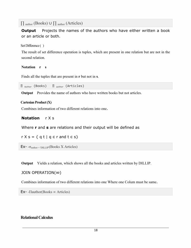
∏ author (Books) ∪ ∏ author (Articles)

Output Projects the names of the authors who have either written a book

or an article or both.

Set Difference ( )

The result of set difference operation is tuples, which are present in one relation but are not in the

second relation.

Notation r s

Finds all the tuples that are present in r but not in s.

∏ Author (Books) ∏ author (Articles)

Output Provides the name of authors who have written books but not articles.

Cartesian Product (Χ)

Combines information of two different relations into one.

Notation r Χ s

Where r and s are relations and their output will be defined as

r Χ s = { q t | q ∈ r and t ∈ s}

Ex- -σauthor = 'DILLIP'(Books Χ Articles)

Output Yields a relation, which shows all the books and articles written by DILLIP.

JOIN OPERATION(∞)

Combines information of two different relations into one Where one Colum must be same.

Ex- -Πauthor(Books ∞ Articles)

Relational Calculus

19

In contrast to Relational Algebra, Relational Calculus is a non-procedural query language, that is,

it tells what to do but never explains how to do it.

Relational calculus exists in two forms

Tuple Relational Calculus (TRC)

Filtering variable ranges over tuples

Notation {T | Condition}

Returns all tuples T that satisfies a condition.

For example

{ T.name | Author(T) AND T.article = 'database' }

Output Returns tuples with 'name' from Author who has written article on 'database'.

TRC can be quantified. We can use Existential (∃) and Universal Quantifiers

(∀).

For example

{ R| ∃T ∈ Authors(T.article='database' AND R.name=T.name)}

Output The above query will yield the same result as the previous one.

Domain Relational Calculus (DRC)

In DRC, the filtering variable uses the domain of attributes instead of entire tuple values.

Notation

{a1, a2, a3, ..., an | P (a1, a2, a3, ... ,an)}

Where a1, a2 are attributes and P stands for formulae built by inner attributes.

For example

{< article, page, subject > | ∈ book ∧ subject = 'database'}

Output Yields Article, Page, and Subject from the relation book, where subject is database.

5.SQL

SQL can execute queries against a database

20

SQL can retrieve data from a database SQL can insert records in a database SQL can update records in a database SQL can delete records from a database SQL can create new tables in a database

SQL can set permissions on tables, procedures, and views

SQL CREATE TABLE Syntax

CREATE TABLE table_name ( column_name1 data_type(size), column_name2 data_type(size), column_name3 data_type(size), .... );

Example-1

CREATE TABLE Persons ( PersonID int, LastName varchar (255), FirstName varchar (255), Address varchar (255), City varchar (255) );

SQL SELECT Syntax

SELECT column_name, column_name FROM table_name;

Example-2

SELECT CustomerName, City FROM Customers;

SQL WHERE Syntax

SELECT column_name, column_name FROM table_name WHERE column_name operator value;

Example-3

SELECT * FROM Customers WHERE Country='INDIA';

SQL INSERT INTO Syntax

INSERT INTO table_name (column1, column2, column3,) VALUES (value1, value2, value3,...);

21

Example-4

INSERT INTO Customers (CustomerName, ContactName, Address, City, PostalCode, Country) VALUES ('Cardinal','Tom B. Erichsen','Skagen 21','Stavanger','4006','Norway');

SQL UPDATE Statement

Example-5

Change the value of the "City" column of a record in the "Customers" table:

UPDATE Customers

SET City='BHAWANIPATNA'

WHERE CustomerID=1;

SQL DELETE Syntax

DELETE FROM table_name WHERE some_column=some_value;

Example-6

DELETE FROM Customers WHERE CustomerName='DILLIP' ;

SQL JOIN

An SQL JOIN clause is used to combine rows from two or more tables, based on a common field between them.

Different SQL JOINs

INNER JOIN: Returns all rows when there is at least one match in BOTH tables LEFT JOIN: Return all rows from the left table, and the matched rows from the right table RIGHT JOIN: Return all rows from the right table, and the matched rows from the left

table FULL JOIN: Return all rows when there is a match in ONE of the tables

Example-7

SELECT Customers.CustomerName, Orders.OrderID FROM Customers, Orders where Customers.CustomerID=Orders.CustomerID ORDER BY Customers.CustomerName;

22

SQL DROP INDEX, DROP TABLE, and DROP DATABASE

DROP TABLE table_name

DROP DATABASE database_name

SQL ALTER TABLE Syntax

ALTER TABLE table_name ADD column_name datatype