Lecture XII

Aggregate supply, inflation and Phillips curve

XII.1. Short- and long-term

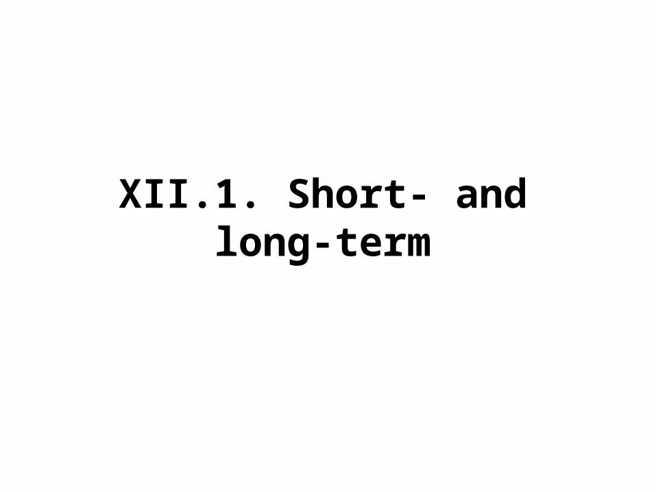
Lecture II – VIII: long-term static model

• All assumptions of a general equilibrium model fulfilled: flexible prices (and wages), full information, etc.

• Long-term enough for prices to adjust and markets to clear

• Aggregate supply vertical, level of (potential) product determined by production function

• Aggregate demand is a decreasing function of price• Say`s law ensures that AD equals AS• Classical dichotomy – amount of money determines

prices (and all other nominal values), but not real variables

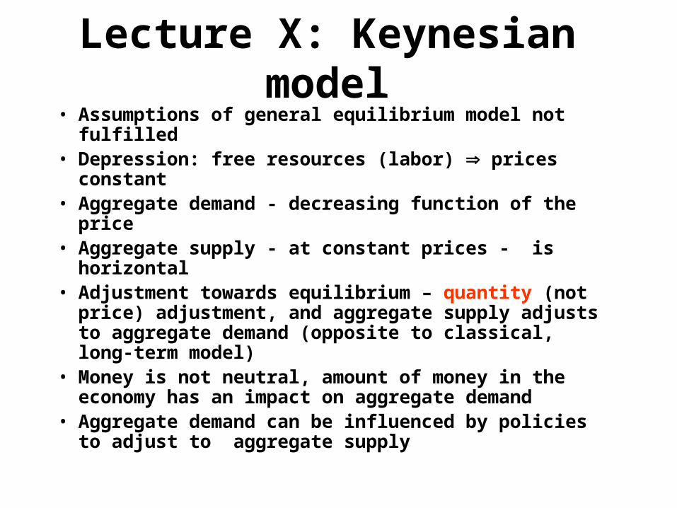
Lecture X: Keynesian model• Assumptions of general equilibrium model not fulfilled• Depression: free resources (labor) prices constant• Aggregate demand - decreasing function of the price • Aggregate supply - at constant prices - is horizontal• Adjustment towards equilibrium – quantity (not price)

adjustment, and aggregate supply adjusts to aggregate demand (opposite to classical, long-term model)

• Money is not neutral, amount of money in the economy has an impact on aggregate demand

• Aggregate demand can be influenced by policies to adjust to aggregate supply

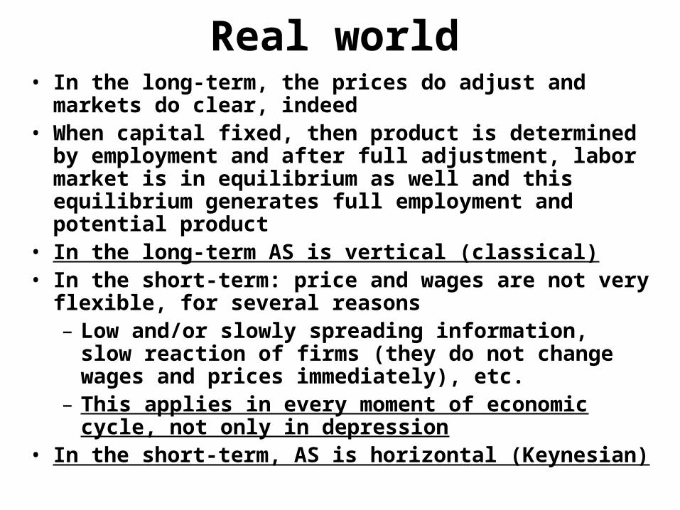
Real world• In the long-term, the prices do adjust and markets do clear,

indeed• When capital fixed, then product is determined by

employment and after full adjustment, labor market is in equilibrium as well and this equilibrium generates full employment and potential product

• In the long-term AS is vertical (classical)• In the short-term: price and wages are not very flexible, for

several reasons– Low and/or slowly spreading information, slow reaction of

firms (they do not change wages and prices immediately), etc.

– This applies in every moment of economic cycle, not only in depression

• In the short-term, AS is horizontal (Keynesian)

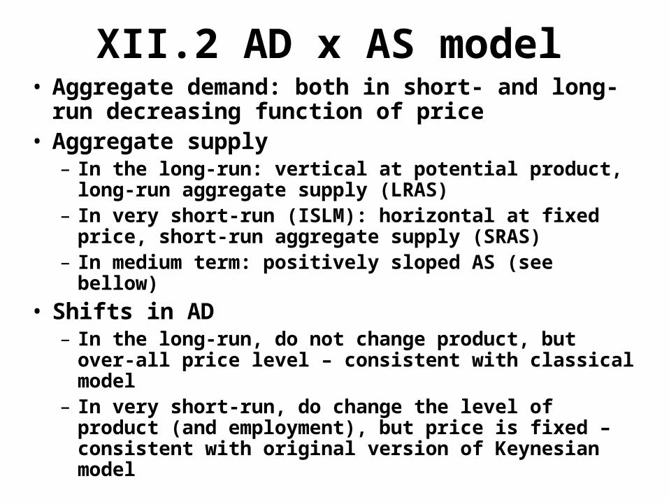
XII.2 AD x AS model• Aggregate demand: both in short- and long-run

decreasing function of price• Aggregate supply

– In the long-run: vertical at potential product, long-run aggregate supply (LRAS)

– In very short-run (ISLM): horizontal at fixed price, short-run aggregate supply (SRAS)

– In medium term: positively sloped AS (see bellow)

• Shifts in AD– In the long-run, do not change product, but over-all price

level – consistent with classical model– In very short-run, do change the level of product (and

employment), but price is fixed – consistent with original version of Keynesian model

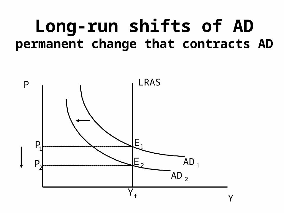
Long-run shifts of ADpermanent change that contracts AD

P

Y

LRAS

AD1

E1

Yf

P1

AD2

E 2

P2

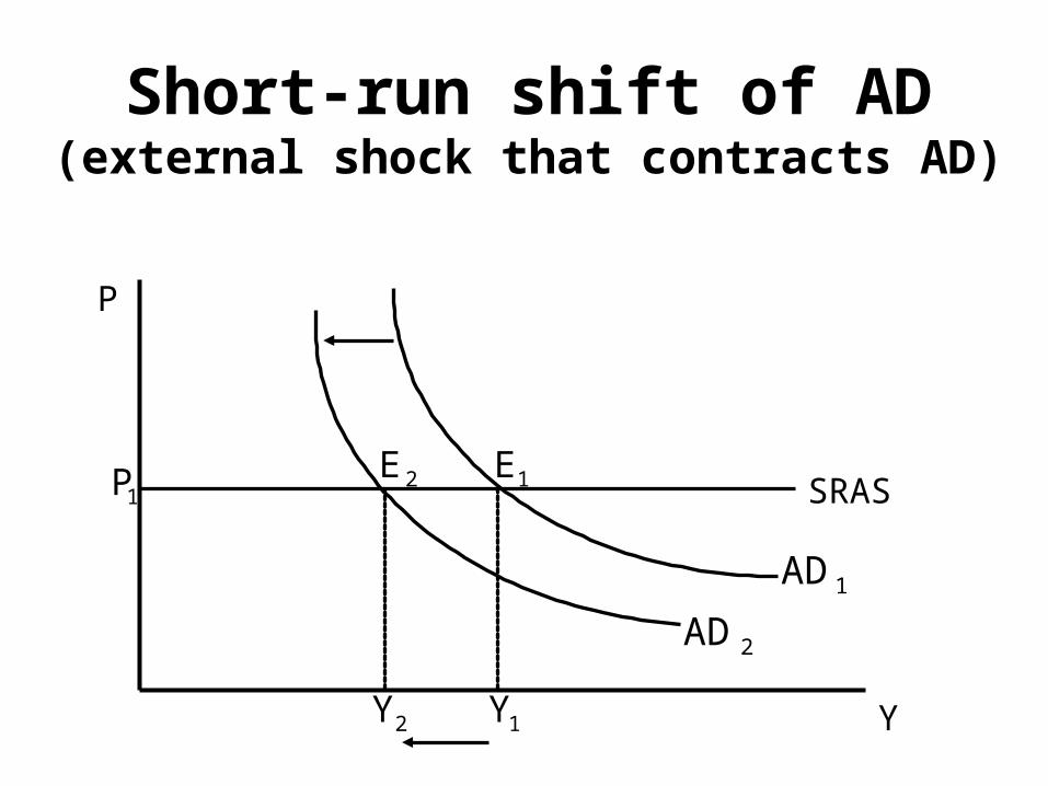
Short-run shift of AD(external shock that contracts AD)

P

Y

SRAS

P1

AD1

Y1

AD2

E1

Y2

E 2

From short- to long-run (1)

• Short-run equilibrium:– AD equals AS, adjustment through quantities AS adjusts to

AD

– Price fixed, equilibrium as state of rest, there can be excess supply on labor market (involuntary unemployment)

– Actual product can be lower/higher than potential one

• Long-run equilibrium:– AD equals AS

– Simultaneous adjustment of all prices generates equilibrium on all markets

– Actual product equal to potential one

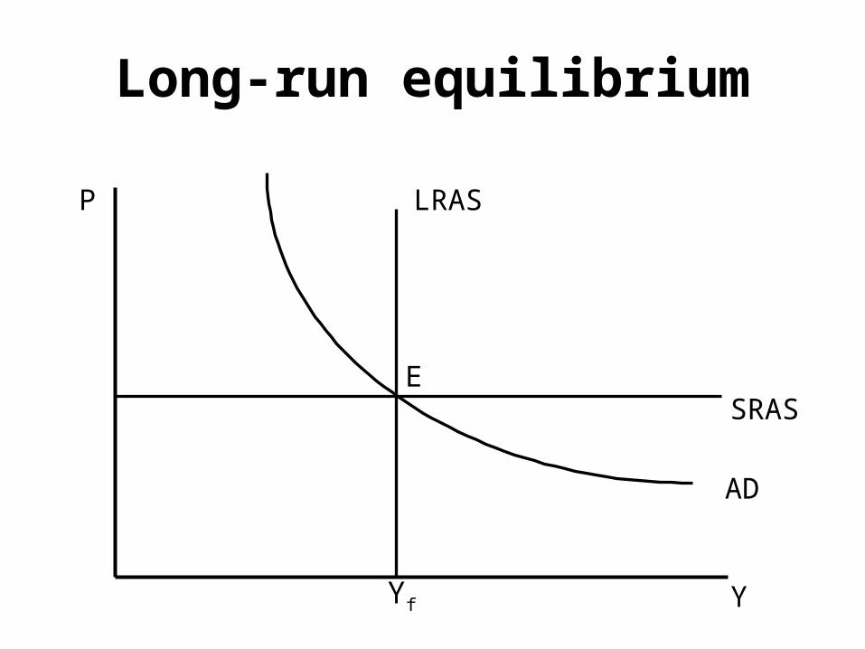
P

Y

LRAS

SRAS

AD

Long-run equilibrium

Yf

E

From short- to long-run (2)

Intuitive interpretation:

• Fixed price corresponds either to the depression (Keynes) or to very short-run, when prices (and wages) are fixed in all economies and at (almost) all situations (exceptions – e.g. hyperinflations)

• Long-run equilibrium – prices and wages had to react to changes in demand/supplies on all markets (including labor) and their adjustment cleared all markets simultaneously

P

Y

LRAS

SRAS1

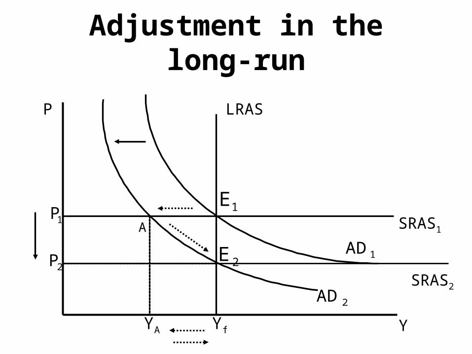
Adjustment in the long-run

Yf

AD1

E1

AD2

A

YA

E 2

P1

P2

SRAS2

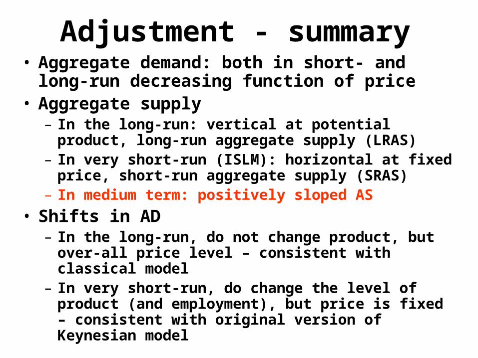
Adjustment - summary• Aggregate demand: both in short- and long-run

decreasing function of price• Aggregate supply

– In the long-run: vertical at potential product, long-run aggregate supply (LRAS)

– In very short-run (ISLM): horizontal at fixed price, short-run aggregate supply (SRAS)

– In medium term: positively sloped AS

• Shifts in AD– In the long-run, do not change product, but over-all price

level – consistent with classical model– In very short-run, do change the level of product (and

employment), but price is fixed – consistent with original version of Keynesian model

XII.3 Short-term aggregate supply

• Adjustment process (from short- to long-term) might take long time an obvious question:– how does the aggregate supply look like in

this adjustment period? increasing function of price

• Model?– No unified theory till today– 3 plausible models, all taking into account

that prices do adjust, but with time lag, slowly (“sticky” prices)

XII.3.1 Wage rigidity –sticky wages

• Originally: F.Modigliani (1944) – downward wage rigidity

• In general: wages rigid in both directions, reasons:– Long term wage contracts, eventually

implicit contracts, power of the unions• Intuitively: if wages rigid, then price increase

lowers real wage firms increase employment product increases and supply increasing function of the price

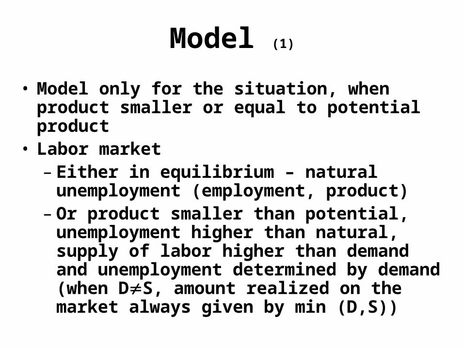
Model (1)

• Model only for the situation, when product smaller or equal to potential product

• Labor market– Either in equilibrium – natural unemployment

(employment, product)– Or product smaller than potential,

unemployment higher than natural, supply of labor higher than demand and unemployment determined by demand (when DS, amount realized on the market always given by min (D,S))

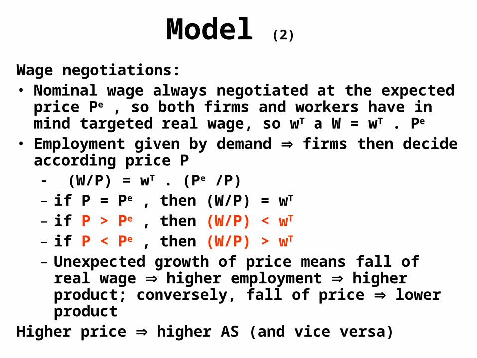
Model (2)

Wage negotiations:• Nominal wage always negotiated at the expected price Pe , so

both firms and workers have in mind targeted real wage, so wT a W = wT . Pe

• Employment given by demand firms then decide according price P- (W/P) = wT . (Pe /P)– if P = Pe , then (W/P) = wT – if P > Pe , then (W/P) < wT – if P < Pe , then (W/P) > wT – Unexpected growth of price means fall of real wage

higher employment higher product; conversely, fall of price lower product

Higher price higher AS (and vice versa)

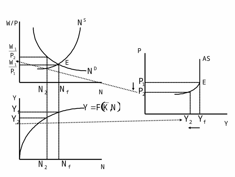
N

W/P

ND

NS

E

N f

W1

P1

N

Y

Y F K,N

N f

Yf

Y

P

Yf

P1

P2

W1

P2

N2

N2

Y2

Y2

AS

E

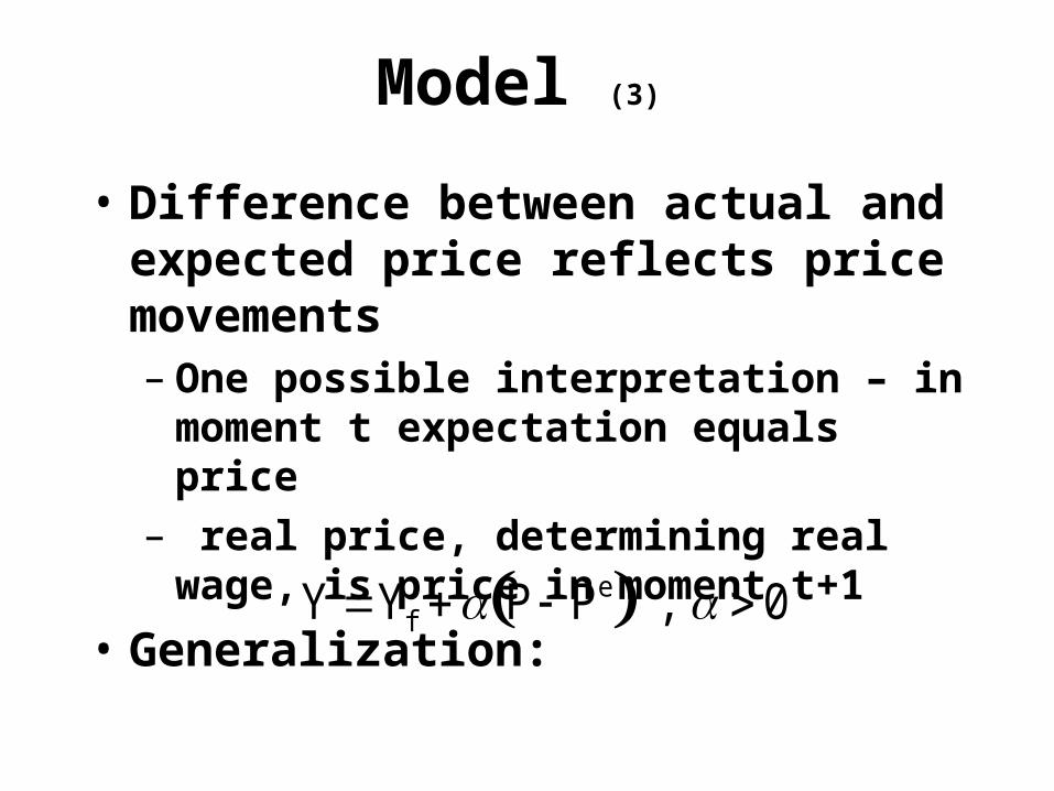
Model (3)

• Difference between actual and expected price reflects price movements– One possible interpretation – in moment t

expectation equals price– real price, determining real wage, is price in

moment t+1

• Generalization:

Y Yf P Pe , 0

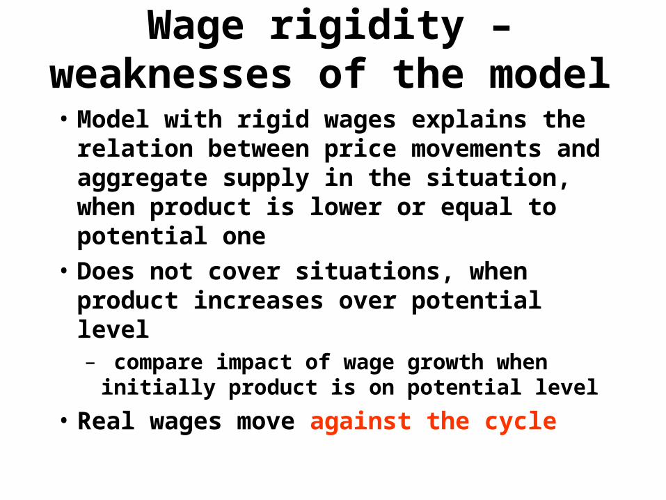
Wage rigidity – weaknesses of the model

• Model with rigid wages explains the relation between price movements and aggregate supply in the situation, when product is lower or equal to potential one

• Does not cover situations, when product increases over potential level– compare impact of wage growth when

initially product is on potential level

• Real wages move against the cycle

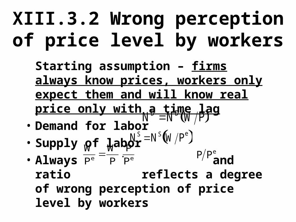
XIII.3.2 Wrong perception of price level by workers

Starting assumption – firms always know prices, workers only expect them and will know real price only with a time lag

• Demand for labor

• Supply of labor

• Always and ratio reflects a degree of wrong perception of price level by workers

ND ND W P

NS NS W Pe

W

Pe

W

P.

P

Pe

P Pe

Model (1)

• Demand for labor: decreasing function of real wage

• Supply of labor: increasing function of expected real wage, can be written as

– Labor supply curve shifts according the ratio P/Pe

• Model explains the relation between price and AS even when product is higher than a potential one

• Model assumes simultaneous clearing of all markets

NS NS W Pe NS W P . P Pe

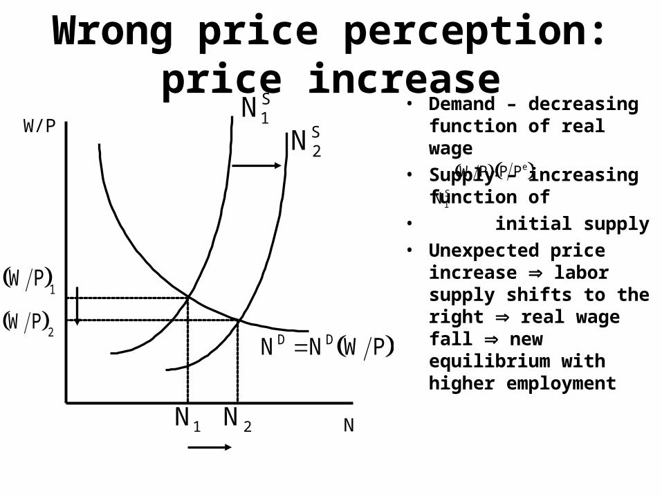
Wrong price perception: price increase

• Demand – decreasing function of real wage

• Supply – increasing function of

• initial supply

• Unexpected price increase labor supply shifts to the right real wage fall new equilibrium with higher employment

N

W/P

ND ND W P

N1S

W P . P Pe

N1S

N2S

W P 1

N1

N2

W P 2

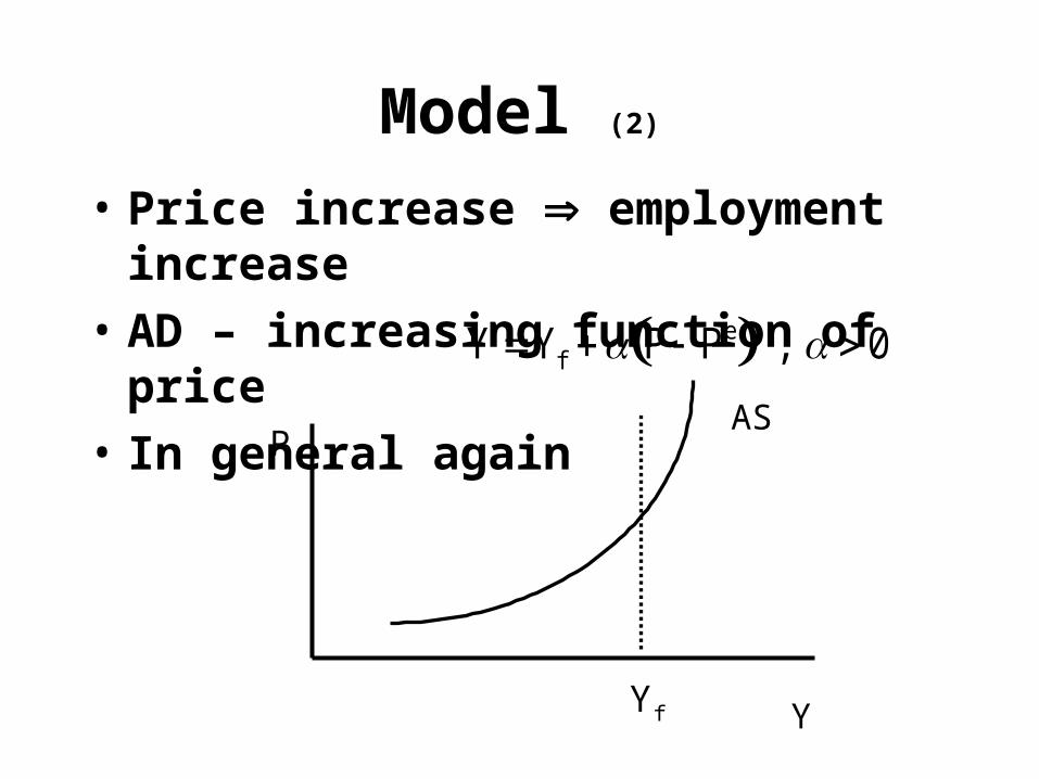
Model (2)

• Price increase employment increase

• AD – increasing function of price

• In general again

Y Yf P Pe , 0

P

Y

AS

fY

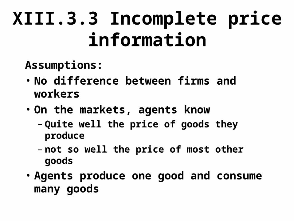
XIII.3.3 Incomplete price information

Assumptions:

• No difference between firms and workers

• On the markets, agents know– Quite well the price of goods they produce– not so well the price of most other goods

• Agents produce one good and consume many goods

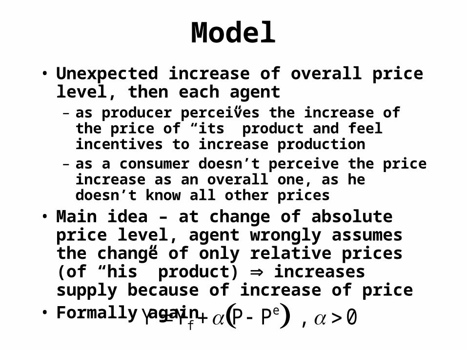
Model• Unexpected increase of overall price level, then

each agent– as producer perceives the increase of the price of

“its” product and feel incentives to increase production

– as a consumer doesn’t perceive the price increase as an overall one, as he doesn’t know all other prices

• Main idea – at change of absolute price level, agent wrongly assumes the change of only relative prices (of “his” product) increases supply because of increase of price

• Formally again

Y Yf P Pe , 0

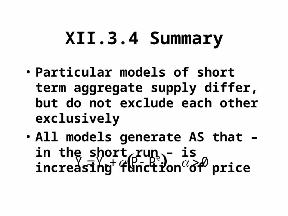
XII.3.4 Summary

• Particular models of short term aggregate supply differ, but do not exclude each other exclusively

• All models generate AS that – in the short run – is increasing function of price

Y Yf P Pe , 0

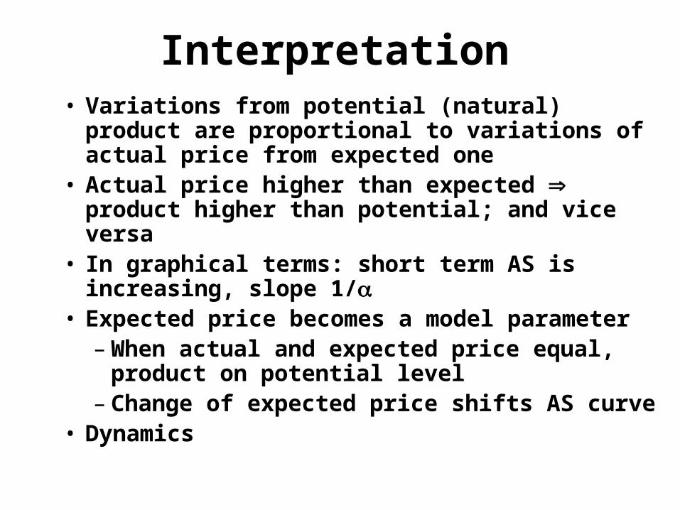
Interpretation• Variations from potential (natural) product are

proportional to variations of actual price from expected one

• Actual price higher than expected product higher than potential; and vice versa

• In graphical terms: short term AS is increasing, slope 1/

• Expected price becomes a model parameter– When actual and expected price equal, product

on potential level– Change of expected price shifts AS curve

• Dynamics

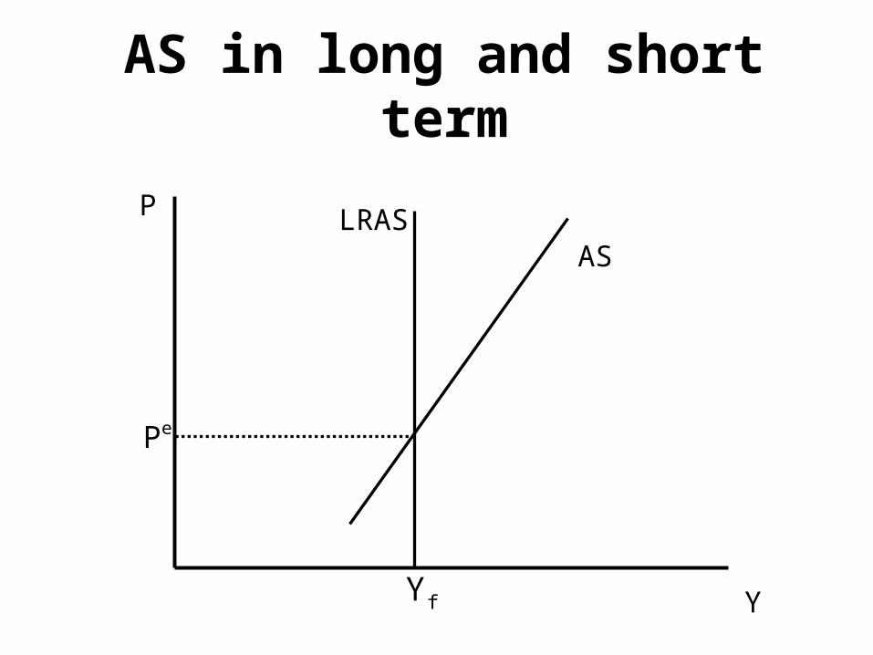
AS in long and short term

Y

P LRASAS

fY

eP

XII.4 Model AD-AS

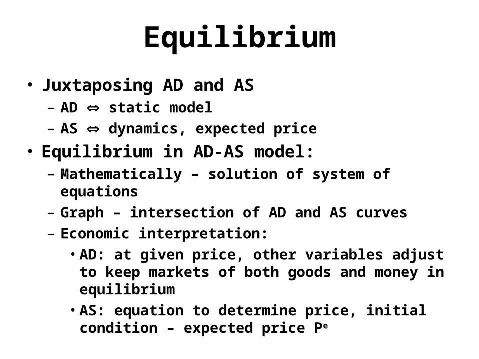
Equilibrium

• Juxtaposing AD and AS– AD static model

– AS dynamics, expected price

• Equilibrium in AD-AS model:– Mathematically – solution of system of equations

– Graph – intersection of AD and AS curves

– Economic interpretation:

• AD: at given price, other variables adjust to keep markets of both goods and money in equilibrium

• AS: equation to determine price, initial condition – expected price Pe

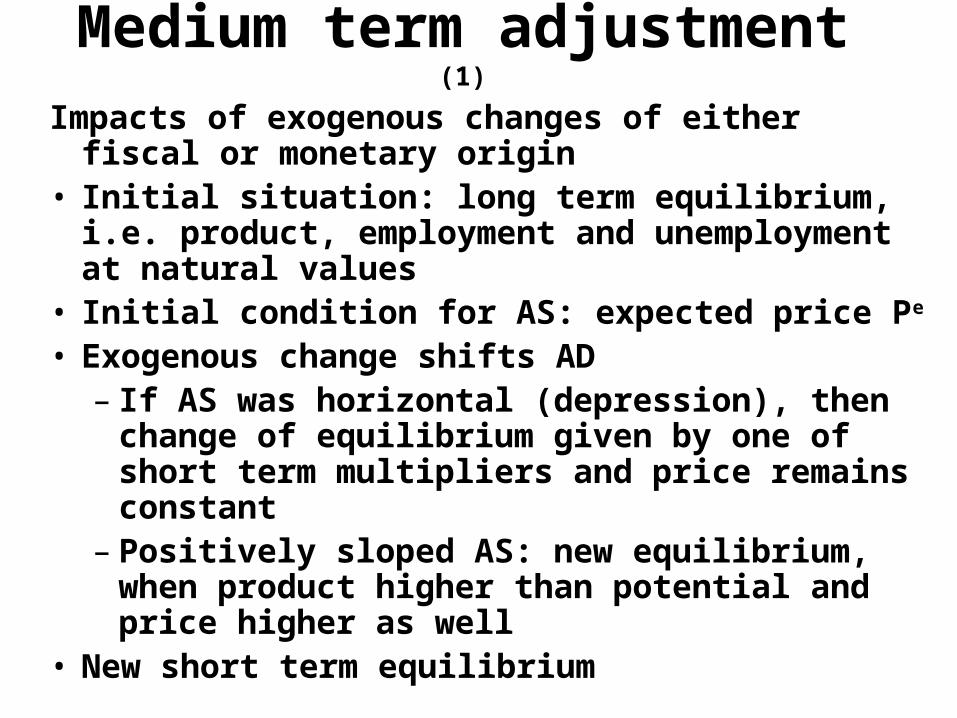
Medium term adjustment (1)

Impacts of exogenous changes of either fiscal or monetary origin

• Initial situation: long term equilibrium, i.e. product, employment and unemployment at natural values

• Initial condition for AS: expected price Pe

• Exogenous change shifts AD– If AS was horizontal (depression), then change of

equilibrium given by one of short term multipliers and price remains constant

– Positively sloped AS: new equilibrium, when product higher than potential and price higher as well

• New short term equilibrium

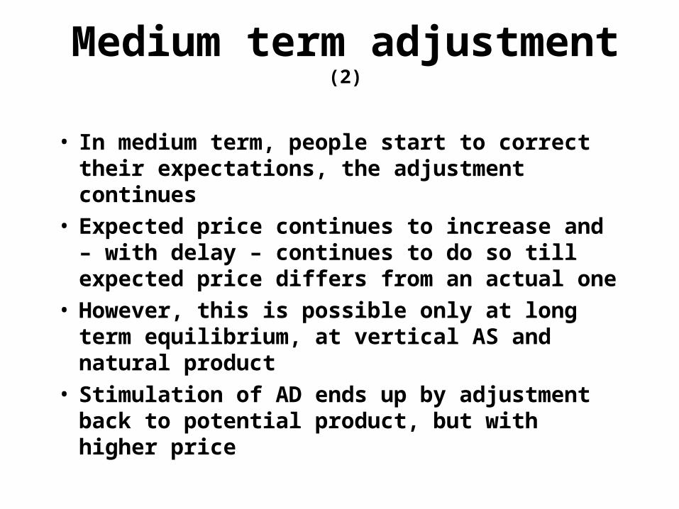
Medium term adjustment (2)

• In medium term, people start to correct their expectations, the adjustment continues

• Expected price continues to increase and – with delay – continues to do so till expected price differs from an actual one

• However, this is possible only at long term equilibrium, at vertical AS and natural product

• Stimulation of AD ends up by adjustment back to potential product, but with higher price

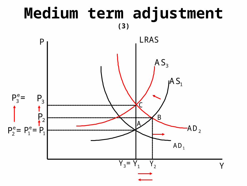
Medium term adjustment (3)

P

Y

LRAS

Y1

P1e = P1

A

AD1

AS1

AD2

Y2

P2

AS3

B

C

Y3=

P3

P2e =

P3e =

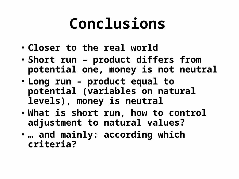
Conclusions

• Closer to the real world• Short run – product differs from

potential one, money is not neutral• Long run – product equal to potential

(variables on natural levels), money is neutral

• What is short run, how to control adjustment to natural values?

• … and mainly: according which criteria?

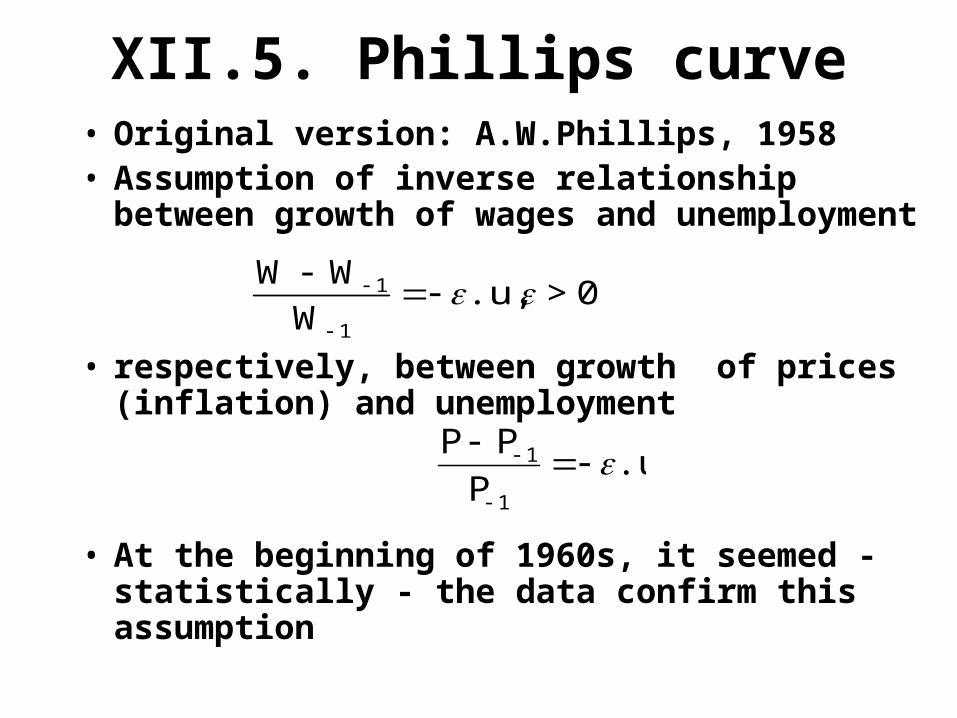
XII.5. Phillips curve• Original version: A.W.Phillips, 1958• Assumption of inverse relationship between

growth of wages and unemployment

• respectively, between growth of prices (inflation) and unemployment

• At the beginning of 1960s, it seemed - statistically - the data confirm this assumption

W W 1

W 1

.u, > 0

P P 1

P 1

.u

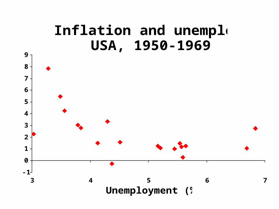
Inflation and unemploymentUSA, 1950-1969

-1

0

1

2

3

4

5

6

7

8

9

3 4 5 6 7

Unemployment (%)

Infl

atio

n (

%)

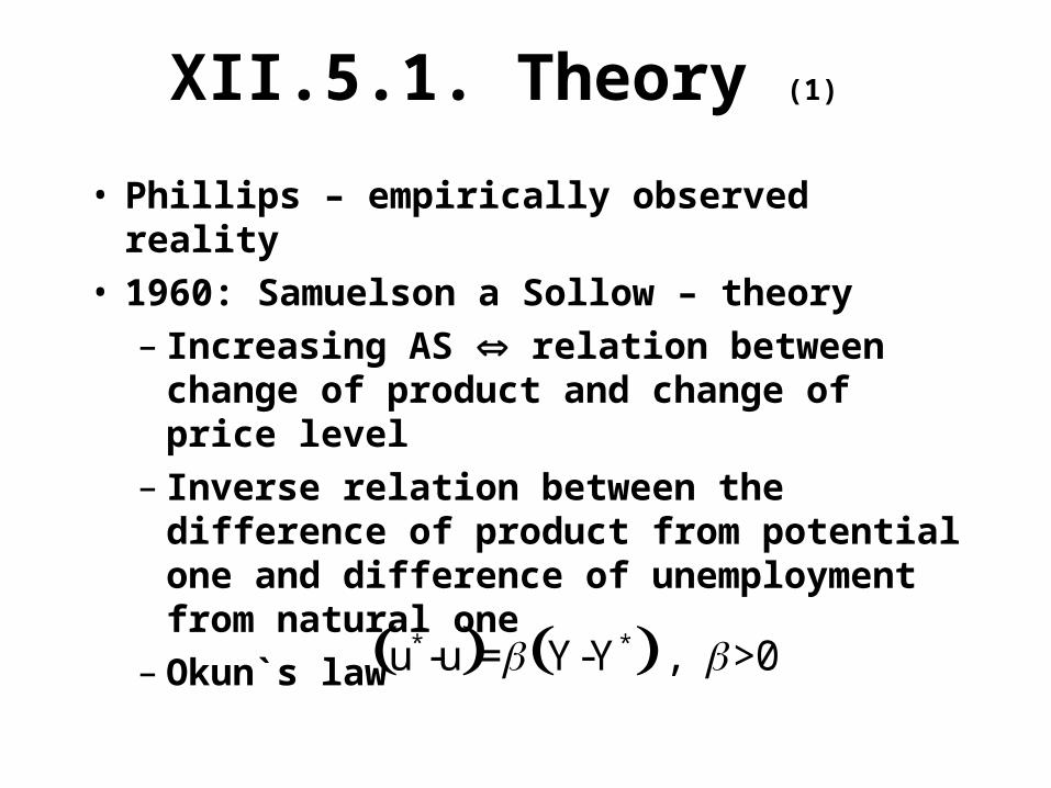
XII.5.1. Theory (1)

• Phillips – empirically observed reality• 1960: Samuelson a Sollow – theory

– Increasing AS relation between change of product and change of price level

– Inverse relation between the difference of product from potential one and difference of unemployment from natural one

– Okun`s law

u*-u = Y-Y* , >0

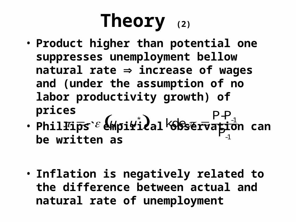
Theory (2)

• Product higher than potential one suppresses unemployment bellow natural rate increase of wages and (under the assumption of no labor productivity growth) of prices

• Phillips` empirical observation can be written as

• Inflation is negatively related to the difference between actual and natural rate of unemployment

. u u* , kde P-P-1

P-1

Inflation

• L V – inflation defined as a monetary phenomenon

• Here – theory, based on an empirically observed Phillips` curve

• Original version of Phillips curve – theory of demand-pull inflation, i.e. inflation, generated by the increase of aggregate demand, that decreases unemployment bellow a natural level, with subsequent increase of nominal wages and price

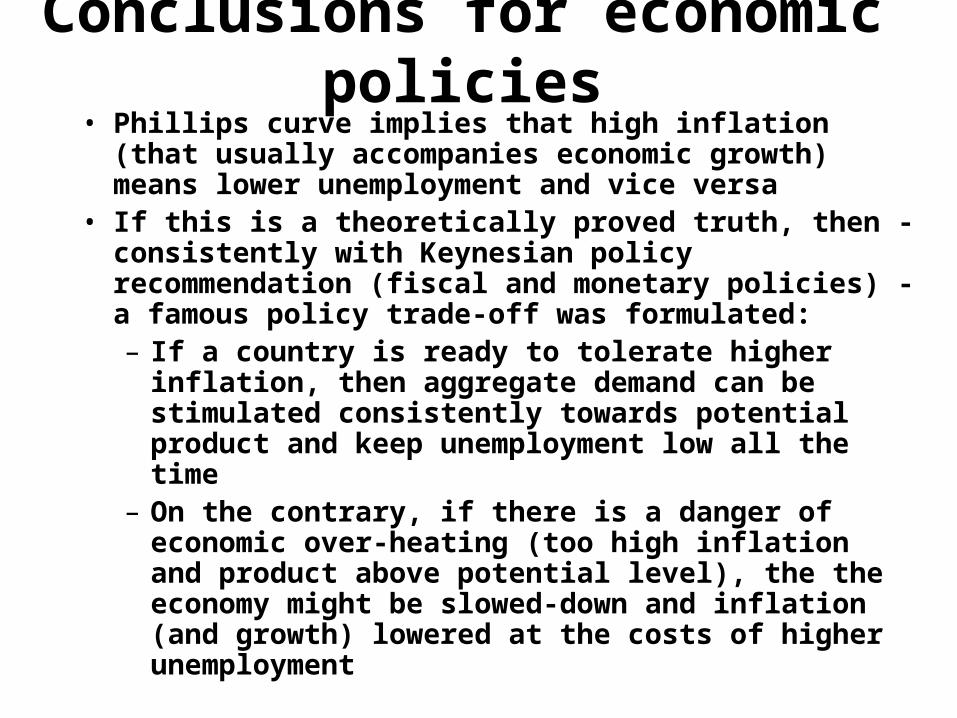
Conclusions for economic policies• Phillips curve implies that high inflation (that usually

accompanies economic growth) means lower unemployment and vice versa

• If this is a theoretically proved truth, then - consistently with Keynesian policy recommendation (fiscal and monetary policies) - a famous policy trade-off was formulated: – If a country is ready to tolerate higher inflation, then

aggregate demand can be stimulated consistently towards potential product and keep unemployment low all the time

– On the contrary, if there is a danger of economic over-heating (too high inflation and product above potential level), the the economy might be slowed-down and inflation (and growth) lowered at the costs of higher unemployment

XII.5.2. Empirical problems and inflationary expectations

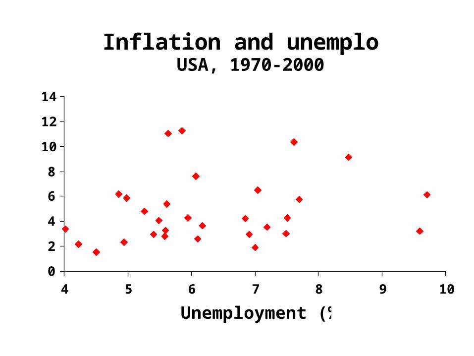
Inflation and unemploymentUSA, 1970-2000

0

2

4

6

8

10

12

14

4 5 6 7 8 9 10

Unemployment (%)

Infl

atio

n (%

)

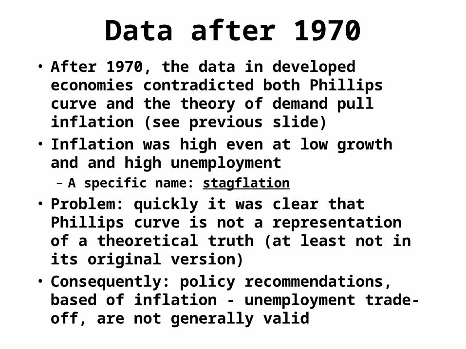
Data after 1970• After 1970, the data in developed economies

contradicted both Phillips curve and the theory of demand pull inflation (see previous slide)

• Inflation was high even at low growth and and high unemployment – A specific name: stagflation

• Problem: quickly it was clear that Phillips curve is not a representation of a theoretical truth (at least not in its original version)

• Consequently: policy recommendations, based of inflation - unemployment trade-off, are not generally valid

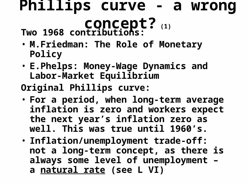
Phillips curve - a wrong concept? (1)

Two 1968 contributions:• M.Friedman: The Role of Monetary Policy• E.Phelps: Money-Wage Dynamics and Labor-

Market EquilibriumOriginal Phillips curve:• For a period, when long-term average inflation

is zero and workers expect the next year’s inflation zero as well. This was true until 1960’s.

• Inflation/unemployment trade-off: not a long-term concept, as there is always some level of unemployment – a natural rate (see L VI)

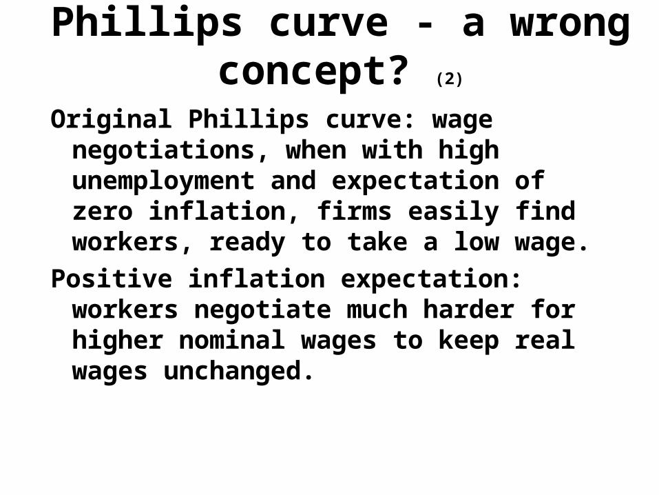
Phillips curve - a wrong concept? (2)

Original Phillips curve: wage negotiations, when with high unemployment and expectation of zero inflation, firms easily find workers, ready to take a low wage.

Positive inflation expectation: workers negotiate much harder for higher nominal wages to keep real wages unchanged.

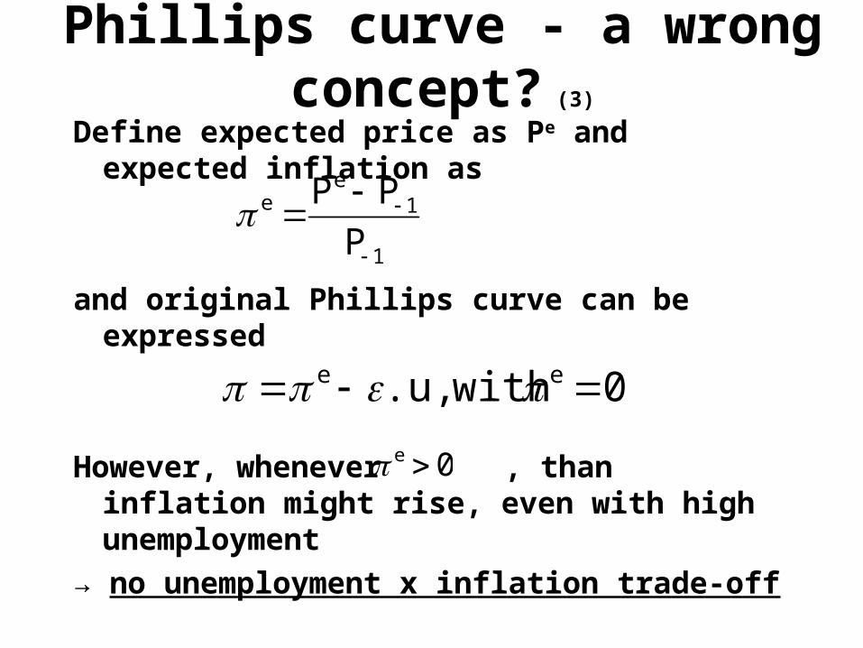
Phillips curve - a wrong concept? (3)

Define expected price as Pe and expected inflation as

and original Phillips curve can be expressed

However, whenever , than inflation might rise, even with high unemployment

→ no unemployment x inflation trade-off

e Pe P 1

P 1

e .u, with e 0

e 0

Phillips curve - a wrong concept? (4)

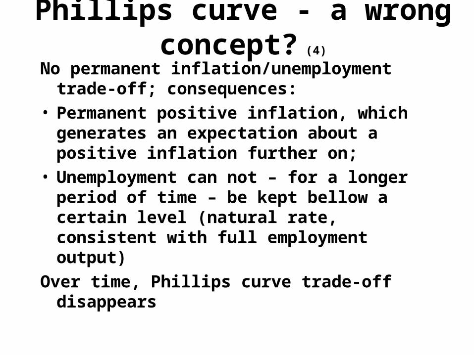
No permanent inflation/unemployment trade-off; consequences:

• Permanent positive inflation, which generates an expectation about a positive inflation further on;

• Unemployment can not – for a longer period of time – be kept bellow a certain level (natural rate, consistent with full employment output)

Over time, Phillips curve trade-off disappears

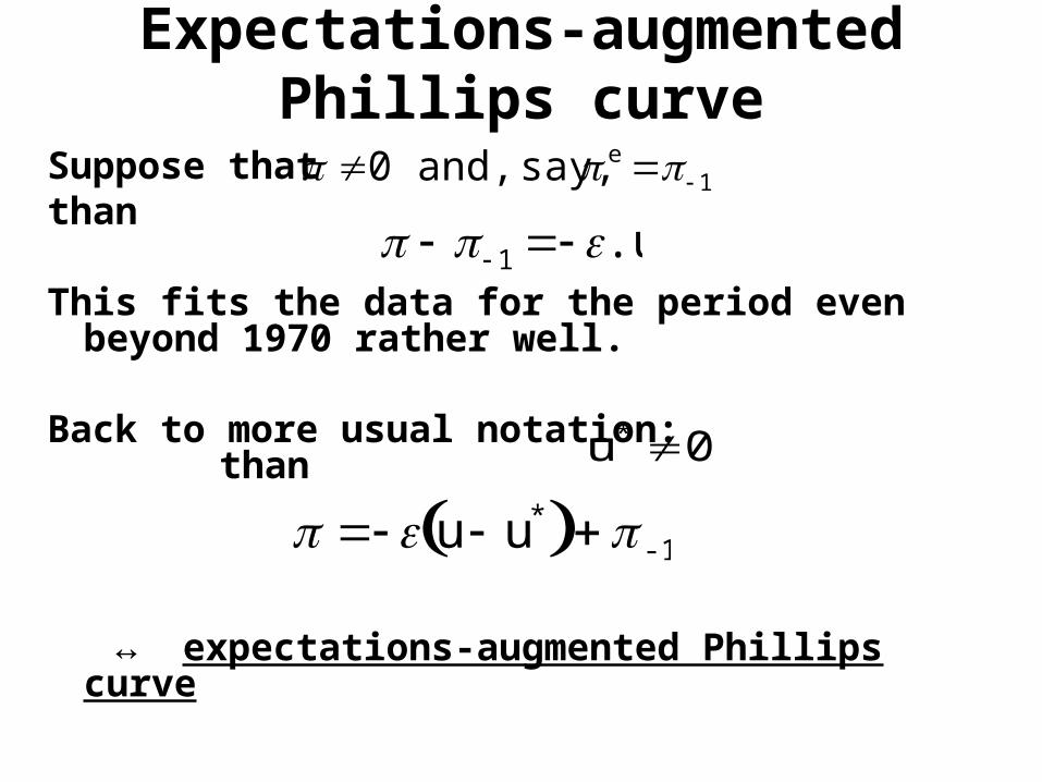
Expectations-augmented Phillips curve

Suppose thatthan

This fits the data for the period even beyond 1970 rather well.

Back to more usual notation: than

↔ expectations-augmented Phillips curve

0 and, say, e 1

1 .u

0u*

u u* -1

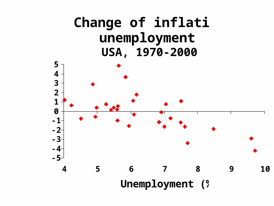
Change of inflation and unemploymentUSA, 1970-2000

-5-4-3-2-1012345

4 5 6 7 8 9 10

Unemployment (%)

Ch

ange

of

infl

atio

n

(%)

XII.5.3. Cost-push inflation• Even without demand pressures, economy

might suffer from even higher inflation because of increase of costs

• Usually as a consequence of exogenous shocks– Oil socks in 1970s

• Consequences for economic policies, dilemma– Either prevent higher inflationary expectations, but

at the cost of temporary slow-down in economic growth and increase of unemployment

– Or stimulate aggregate demand, overcome stagnation, but inflation will not only be higher, but higher inflationary expectations will be generated

Literature to L XII

• Mankiw, Ch. 9

• Holman, Ch. 10