Fitting to a set of data

Lecture on fitting

Linear regression

● Linear regression

– Residual is the amount difference between a real data point and a modeled data point

– Fitting a polynomial to data

● Could use minimization of the sum of residuals

– Cancellation errors– Could bisect a set of points rather than fitting through them

● Could use minimization of the sum of the absolute value of the residuals

– Too much influence to outliers● Could use minimization of the sum of the square of the residuals

– Works well– Solves problems mention in the other two methods

Least square

● Least square form, take derivative

S=∑i=1

n

yi ,measured−yi,model2

S=∑i=1

n

yi−ao−a1xi2

∂S∂a0

=−2∑ yi−a0−a1xi=0

∂S∂a1

=−2∑ yi−a0−a1x1xi=0

ymodel=mxib=a0a1xi

slope=a1=n∑ xiyi−∑ xi∑ yi

n∑ xi2−∑xi

2

ao=⟨y⟩−a1⟨x⟩

Polyfit (from Octave)Take some data x,y (error sy)

Fit line using polyfit as so

>>[a,b] = polyfit(x,y,1)

>>plot(x,y,'*')

>>Line = a(1)*x+a(2)

>>Hold on

>>plot(x,line,'-+g')

- or more professionally -

>>[p,s] = wpolyfit(x,y,sy,1)

>>[yn,syn]=polyconf(p,x,s,'ci')

>> plot(x,yn,'gd-')

Nonlinear regression

● Cannot solve like the least square method– Use Gauss-Newton optimization method

● Think Levenberg-Marquardt which is an optimization method of this nature

● Think least square/minimization/idea/concept

Interpolation

>>slope = (y(5)-y(4))/(x(5)-x(4))

>>intercept=y(4)-slope*x(4)

>>newline=slope*x+intercept

>>plot(x,y,'*')

>> hold on

>>plot(x(4:5),newline(4:5))

>>%% Clearly I can now get a point

>>%% in the middle

>>point=slope*3.4+intercept

This is a simple way of interpolating clearly it could be argued that a fitted line would be more appropriate than a slope-intercept form.

Splines are often used

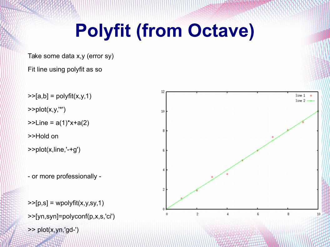
Extrapolation>>slope = (y(5)-y(4))/(x(5)-x(4))

>>intercept=y(4)-slope*x(4)

>> %% xx is x extended

>>newline=slope*xx+intercept

>>plot(x,y,'*')

>> hold on

>>plot(xx(10:12),newline2(10:12))

>>%% Clearly I can now get a point

>>%% in the beyond the data

>>point=slope*10.6+intercept

This is a simple way of extrapolation clearly it could be argued that a fitted line would be more appropriate than a slope-intercept form.

Splines are often used

Spline

● Fits splines (curves) through the data

– Fits data (usually noisy) through “knots” ● Good method

● Requires picking knot locations

– Fits through knots using best method

– Use a “spline” like in boats to fit through the points (or knots)

– Different curves can be generated depending on the type of spline used

– B-spline is popular● B in B-spline stands for “basis” functions

● Curves of the B-spline have orders which progressively look like a line to a “triangular hat” to an actual curve

● Other splines include the cubic, Bezier, etc.

– T-spline is a terminated non-recursive rational B-spline● This is why you see both t-spline and b-spline calculated in the same

function

SplineB-spline basic functions (image from Berkeley)

Digital Filters

● In essence an electronic filter that is represented digitally

– Control systems (or system dynamics)● Convert a signal to a digital signal● Change the signal using a transfer function over the

digital signal● Implemented using a difference equation

– Like a Fast Fourier Transform (FFT)

– Used for smoothing

– Used for fitting

– While advantageous over electronic filtering due to the inherent drifts and noise, it can be very complex and lead to removal of real signal

Digital Filters

● There are a number of types of digital filters thought they all revolve around some form of transfer function– IIR filters

● Infinite impulse response (delta functions) filters

– Dirac delta functions– Mathematically ideal– Need to implement carefully around “x=0”

point as there is no clear definition of what that is...can do it though

– Typically defined carefully with a difference equation

∫−∞

∞

f x x−adx= f a

Digital Filters

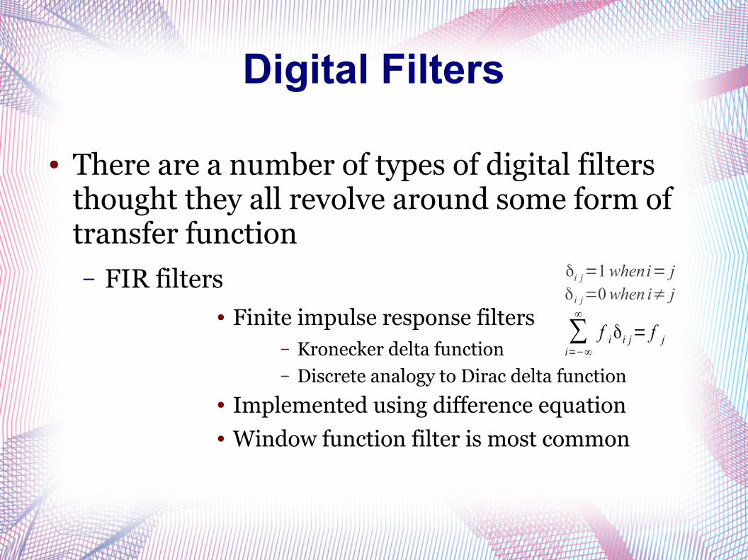
● There are a number of types of digital filters thought they all revolve around some form of transfer function– FIR filters

● Finite impulse response filters– Kronecker delta function– Discrete analogy to Dirac delta function

● Implemented using difference equation● Window function filter is most common

δi j=1wheni= jδi j=0when i≠ j

∑i=−∞

∞

f iδi j= f j

Control Systems - filters

● Control systems (system dynamics)

– Difference equation (possible derived from a transform) equates the output to the input by a set of coefficients that “filter” the input

– Iterative process

– Where coefficients represent feed forward (a coefficients) and feed back (b coefficients) coefficients (recall EGR 1010 discussion of this)

– Equation below is for IIR, remove feedback and you have FIR

yn=α (∑i=0

i=l

ai x i−n−∑j=1

j=m

b j y n− j)