Lecture NotesTime Series Analysis

Summer term 2020Friedrich-Schiller-Universität Jena

Michael H. Neumann

DisclaimerThese lecture notes are for personal use only. Unauthorized reproduction, copying, dis-tribution or any other use of the whole or any part of this document is strictly prohibited.

2

Important information

• Lecture period: May 04 – July 17Prior to a possible start of classroom lectures you will find your weekly program asa corresponding part of lecture notes. You will find the material under the fol-lowing link: https://users.fmi.uni-jena.de/~jschum/lehre/lectures.php?name=Neumann

• Examination period: July 20 – August 14There will be oral examinations, hopefully within the official examination period.Dates of these examinations will be fixed in good time.

• Contact

– Office: room 3516

– Phone: 03641/946260

– Email: michael.neumann@uni-jena.de

Literature[1] Brockwell, P. J. and Davis, R. A. (1991). Time Series: Theory and Methods. 2nd

Edition. Springer. New York.

[2] Kreiß, J.-P. and Neuhaus, G. (2006). Einführung in die Zeitreihenanalyse. Springer.Berlin. (in German)

3

Contents1 Models for time series 4

1.1 Basic concepts, stationarity . . . . . . . . . . . . . . . . . . . . . . . . . 41.2 Hilbert spaces . . . . . . . . . . . . . . . . . . . . . . . . . . . . . . . . . 101.3 Linear processes . . . . . . . . . . . . . . . . . . . . . . . . . . . . . . . . 201.4 Autoregressive processes . . . . . . . . . . . . . . . . . . . . . . . . . . . 221.5 ARMA processes . . . . . . . . . . . . . . . . . . . . . . . . . . . . . . . 22

2 Spectral analysis of stationary processes 222.1 Spectral density, spectral distribution function . . . . . . . . . . . . . . . 222.2 Estimation in the spectral domain . . . . . . . . . . . . . . . . . . . . . . 22

4

1 Models for time seriesWe consider some popular classes of stochastic processes and investigate their properties.Methods of estimating certain parameters will also be considered.

1.1 Basic concepts, stationarity

Definition 1.1. A stochastic process is a family of random variables X = (Xt)t∈Tdefined on a common probability space (Ω,F , P ).For ω ∈ Ω, the function t 7→ Xt(ω) on T is called realization or sample path of theprocess X.The term time series is used for the process X but also for a realization of X.For t1, . . . , tk ∈ T , k ∈ N, PXt1 ,...,Xtk is a finite-dimensional distribution of theprocess X on (Ω,F , P ).

In the following:

• T = N = 1, 2, . . ., T = N0 = 0, 1, 2, . . . or T = Z

• Xt takes values in R or (sometimes) in C or Rd

Consistency of (sequences of) estimators will be possible if we obtain an increasingamount of new information about the underlying situation as the sample sizes tends toinfinity. This is usually the case if the dependence between the observed random variablesis not too strong and if the parameters do not change over time. The latter requirementleads to the important concept of stationarity of a process.

Definition 1.2. Let X = (Xt)t∈Z be a (real-valued) stochastic process on (Ω,F , P ).

(i) X is said to be strictly stationary if

PXt1 ,...,Xtk = PXt1+t,...,Xtk+t ∀t1, . . . , tk, t ∈ Z,∀k ∈ N.

(ii) X is said to be stationary (weakly stationary) if

a) EX2t <∞ ∀t ∈ Z,

b) EXt = µ ∀t ∈ Z and some µ ∈ R,c) cov(Xr, Xs) = cov(Xr+t, Xs+t) ∀r, s, t ∈ Z.

In this case, γX(k) = cov(Xt+k, Xt) is the autocovariance at lag k,γX : Z→ R is the autocovariance function.

If T = N0 or T = N, then the above definition has to be adapted accordingly.

5

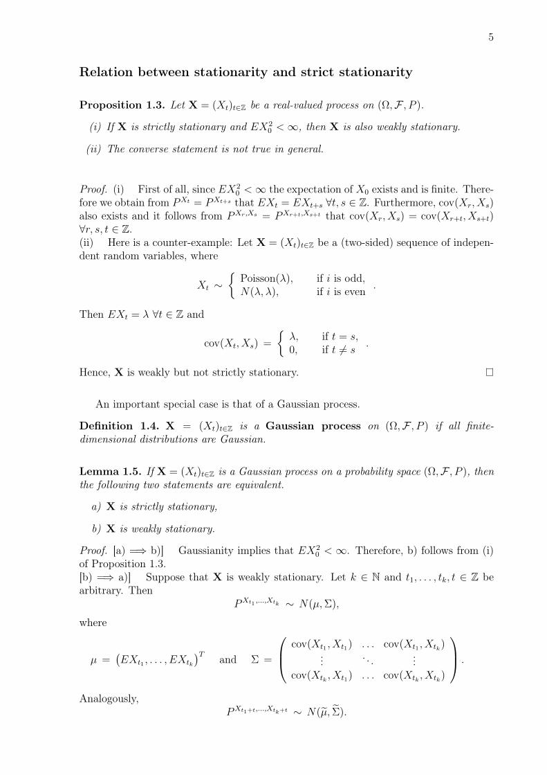
Relation between stationarity and strict stationarity

Proposition 1.3. Let X = (Xt)t∈Z be a real-valued process on (Ω,F , P ).

(i) If X is strictly stationary and EX20 <∞, then X is also weakly stationary.

(ii) The converse statement is not true in general.

Proof. (i) First of all, since EX20 <∞ the expectation of X0 exists and is finite. There-

fore we obtain from PXt = PXt+s that EXt = EXt+s ∀t, s ∈ Z. Furthermore, cov(Xr, Xs)also exists and it follows from PXr,Xs = PXr+t,Xs+t that cov(Xr, Xs) = cov(Xr+t, Xs+t)∀r, s, t ∈ Z.(ii) Here is a counter-example: Let X = (Xt)t∈Z be a (two-sided) sequence of indepen-dent random variables, where

Xt ∼

Poisson(λ), if i is odd,N(λ, λ), if i is even .

Then EXt = λ ∀t ∈ Z and

cov(Xt, Xs) =

λ, if t = s,0, if t 6= s

.

Hence, X is weakly but not strictly stationary.

An important special case is that of a Gaussian process.

Definition 1.4. X = (Xt)t∈Z is a Gaussian process on (Ω,F , P ) if all finite-dimensional distributions are Gaussian.

Lemma 1.5. If X = (Xt)t∈Z is a Gaussian process on a probability space (Ω,F , P ), thenthe following two statements are equivalent.

a) X is strictly stationary,

b) X is weakly stationary.

Proof. [a) =⇒ b)] Gaussianity implies that EX20 < ∞. Therefore, b) follows from (i)

of Proposition 1.3.[b) =⇒ a)] Suppose that X is weakly stationary. Let k ∈ N and t1, . . . , tk, t ∈ Z bearbitrary. Then

PXt1 ,...,Xtk ∼ N(µ,Σ),

where

µ =(EXt1 , . . . , EXtk

)T and Σ =

cov(Xt1 , Xt1) . . . cov(Xt1 , Xtk)... . . . ...

cov(Xtk , Xt1) . . . cov(Xtk , Xtk)

.

Analogously,PXt1+t,...,Xtk+t ∼ N(µ, Σ).

6

We obtain from weak stationarity that

µ =(EXt1+t, . . . , EXtk+t

)T= µ

and cov(Xti+t, Xtj+t) = cov(Xti , Xtj), which implies that Σ = Σ. Therefore, X is alsostrictly stationary.

Examples

1) Let (εt)t∈Z be a sequence of i.i.d. random variables. This process is (obviously) bothweakly and strictly stationary.

2) Let Y and Z be uncorrelated random variables with EY = EZ = 0 and EY 2 =EZ2 = 1. We define, for any θ ∈ [−π, π],

Xt := Y cos(θt) + Z sin(θt).

ThenEXt = 0 ∀t

and

cov(Xt+r, Xt) = E [Y cos(θ(t+ r)) + Z sin(θ(t+ r)) Y cos(θt) + Z sin(θt)]= cos(θ(t+ r)) cos(θt) + sin(θ(t+ r)) sin(θt)

= cos(θr).

The latter equation holds since, on the one hand,

ei(u−v) = cos(u− v) + i sin(u− v),

and, on the other hand,

ei(u−v) = eiu e−iv =(

cos(u) + i sin(u))(

cos(v) − i sin(v))

= cos(u) cos(v) + sin(u) sin(v) + i(

sin(u) cos(v) − cos(u) sin(v)).

Therefore, the autocovariances are also shift-invariant which means that the process(Xt)t∈Z is weakly stationary.

3) Let X0, ε1, ε2, . . . be independent, X0 ∼ N(0, σ2X), and εt ∼ N(0, σ2

ε) ∀t ∈ N.We define consecutively

Xt := α Xt−1 + εt ∀t ∈ N,

where α is a real constant, |α| < 1.

Question: Is it possible to choose σ2X such that the process (Xt)t∈N is stationary?

SinceX1 = α X0 + ε1 ∼ N(0, α2 σ2

X + σ2ε)

a necessary condition for any kind of stationarity is that σ2X = α2σ2

X +σ2ε , i.e. σ2

X =σ2ε/(1− α2).

7

Suppose that σ2ε > 0 and that σ2

X = σ2ε/(1− α2). We have that

Xt = εt + α Xt−1 = . . . = εt + α εt−1 + . . . + αt−1 ε1 + αk X0.

This means that (Xt)t∈N0 is a zero mean Gaussian process. We obtain, as above,that

var(X0) = var(X1) = . . . = var(Xt) ∀t ∈ N.Furthermore, for k ∈ N, we obtain since Xt, εt+1, . . . εt+k are independent that

cov(Xt+k, Xt) = cov(εt+k + αεt+k−1 + · · ·+ αk−1εt+1 + αkXt, Xt) = αk σ2X .

Hence, (Xt)t∈N0 is a weakly stationary process. Moreover, as a Gaussian process, itis also strictly stationary.

The following lemma contains a few elementary properties of the autocovariance functionof a stationary process.Lemma 1.6. Let γ be the autocovariance function of a real-valued stationary process(Xt)t∈Z. Then(i) γ(0) ≥ 0,

(ii) |γ(r)| ≤ γ(0) ∀r ∈ Z,

(iii) γ(r) = γ(−r) ∀r ∈ Z.

Proof. (i) is a statement of the obvious fact that

γ(0) = var(Xt) ≥ 0.

(ii) is an immediate consequence of the Cauchy-Schwarz (Cauchy-Bunyakovsky-Schwarz)inequality,

|γ(r)| = | cov(Xt+r, Xt)| ≤√

var(Xt+r)√

var(Xt) = γ(0).

Finally, (iii) follows from

γ(r) = cov(Xt+r, Xt) = cov(Xt, Xt+r) = γ(−r).

Remark 1.7. If (Xt)t∈Z is a complex-valued process and E[|Xt|2] <∞ ∀t, then

cov(Xt+r, Xt) := E[(Xt+r − EXt+r) (Xt − EXt)

],

where z denotes the complex conjugate of a complex number z. Since, for a complex-valued random variable Y , |EY | ≤ E|Y |, an analogue of the Cauchy-Schwarz inequalityholds true: ∣∣E[Yt+rY t]

∣∣ ≤ E[|Yt+rY t|

]≤√E[|Yt+r|2]

√E[|Yt|2].

Next we intend to find a characterization of autocovariance functions.Definition 1.8. A real-valued function on the integers, κ : Z → R, is said to be non-negative definite (positive semidefinite) if

n∑i,j=1

ai κ(ti − tj) aj ≥ 0 ∀n ∈ N, ai ∈ R, ti ∈ Z.

8

Theorem 1.9. Let γ : Z → R be a real-valued function. Then the following statementsare equivalent.

(i) γ is the autocovariance function of a stationary process (Xt)t∈Z,

(ii) γ is an even and non-negative definite function.

Proof. [(i) =⇒ (ii)] Assume that γ is the autocovariance function of a stationary processX = (Xt)t∈Z. Then

γ(k) = cov(Xk, X0) = cov(X0, Xk) = γ(−k),

i.e. γ is an even function. Moreover, we have, for arbitrary a1, . . . , an ∈ R, t1, . . . , tn ∈ Z,n ∈ N,

n∑i,j=1

ai γ(ti − tj) aj =n∑

i,j=1

ai cov(Xti , Xtj) aj

=n∑

i,j=1

cov(aiXti , ajXtj) = var( n∑i=1

aiXti

)≥ 0,

i.e., γ is non-negative definite.[(ii) =⇒ (i)] Let γ be an arbitrary even and non-negative definite function. For any

m,n ∈ Z, m ≤ n, we consider the matrix

Γm,n :=

γ(m−m) . . . γ(m− n)... . . . ...

γ(n−m) . . . γ(n− n)

.

Since γ is an even function it follows that Γm,n is a symmetric matrix. Moreover, Γm,nis a non-negative definite matrix. Actually, let c = (cm, . . . , cn)T ∈ Rn−m+1 be arbitrary.Then cTΓm,nc =

∑ni,j=m ciγ(i− j)cj ≥ 0. Hence, Γm,n has the properties of a covariance

matrix. We definePm,n := N(0n−m+1,Γm,n),

where 0k = (0, . . . , 0)T denotes a vector of length k consisting of zeroes. It follows that thefamily of distributions (Pm,n)m≤n satisfies the consistency condition of Kolmogorov’s the-orem. Therefore, there exists a stochastic process X = (Xt)t∈Z on a suitable probabilityspace (Ω,F , P ) such that

PXm,...,Xn = Γm,n.

It follows that the process (Xt)t∈Z is stationary and that

cov(Xt+k, Xt) = γ(k),

as required.

9

Exercises

Ex. 1.1 Suppose that (εt)t∈Z is a sequence of i.i.d. random variables, Eε0 = 0, Eε20 =: σ2

ε <∞, and

Xt := εt + β εt−1.

Is the process (Xt)t∈Z stationary?

Ex. 1.2 Let (βk)k∈Z be a sequence of real numbers with∑∞

k=−∞ β2k < ∞. The function

γ : Z→ R is defined by γ(k) =∑∞

j=−∞ βj+kβj.

Is γ an autocovariance function?

10

1.2 Hilbert spaces

First of all, the contents of this chapter seems to be completely out of place in a courseon time series. But why do we pay attention to such an abstract subject as a Hilbertspace? In what follows we will be faced with the following questions.

(i) As a simple class of models for time series, we consider so-called linear processes.Given an underlying process (εt)t∈Z, we consider a process X = (Xt)t∈Z with

Xt =∞∑k=0

βkεt−k. (1)

This raises the following questions.

– Does the infinite sum on the right-hand side of (1) converge? And if so, inwhich sense?

– What is the covariance structure of (Xt)t∈Z?Of course, cov(

∑mj=0 βjεs−j,

∑mk=0 βkεt−k) can be easily computed since we can

take out the finite sums. But what about cov(∑∞

j=0 βjεs−j,∑∞

k=0 βkεt−k) whereinfinite sums are involved?

Answers to these questions can be easily deduced in the general context of Hilbertspaces.

(ii) Suppose that we observe realizations of random variables X1, . . . , Xn, where (Xt)t∈Nis a stationary process. How can we best predict future values, e.g. Xn+1?We will see that a best linear predictor is given by the orthogonal projection ofX1, . . . , Xn onto Xn+1. This can be reformulated as a projection in an appropri-ate Hilbert space and its characterization is most conveniently derived in such anabstract context.

Definition 1.10. A complex vector space H is said to be an inner-product space(scalar space) if for all x, y ∈ H, there exists a complex number 〈x, y〉, called the innerproduct (scalar product) of x and y, such that

(i) 〈x, x〉 ≥ 0 ∀x ∈ H〈x, x〉 = 0 ⇔ x = 0 (0 denotes the zero element of H.),

(ii) 〈x, y〉 = 〈y, x〉 (The bar denotes complex conjugation.),

(iii) 〈αx, y〉 = α 〈x, y〉 ∀α ∈ C,∀x, y ∈ H,

(iv) 〈x+ y, z〉 = 〈x, z〉 + 〈y, z〉 ∀x, y, z ∈ H.

Remark 1.11. A real vector space H is an inner product space if for all x, y ∈ H thereexists a real number 〈x, y〉 such that suitably adapted versions of (i) to (iv) are satisfied.(Of course, (ii) obviously reduces to 〈x, y〉 = 〈y, x〉 and (iii) has to be satisfied for allreal α.)

11

Examples1) Real Euclidean space Rd

〈x, y〉 =d∑i=1

xi yi

2) Complex Euclidean space Cd

〈x, y〉 =d∑i=1

xi yi

Definition 1.12. Let H be an inner-product space, x ∈ H. The norm of x is defined tobe

‖x‖ :=√〈x, x〉.

Actually, in order to justify the term norm we still have to prove that ‖ · ‖ satisfies allproperties of a norm. In particular, validity of the triangle inequality has be checked.Before we come to this point, we state a few auxiliary results.

Lemma 1.13. (Cauchy-Bunyakovsky-Schwarz inequality)Let H be an inner-product space. Then

(i) |〈x, y〉| ≤ ‖x‖ ‖y‖ ∀x, y ∈ H,

(ii) |〈x, y〉| = ‖x‖ ‖y‖ if and only if ‖y‖2 x = 〈x, y〉 y.

Proof. (i) Using the properties of an inner product we obtain that

0 ≤ 〈‖y‖2 x − 〈x, y〉 y, ‖y‖2 x − 〈x, y〉 y〉= ‖x‖2 ‖y‖4 + 〈x, y〉 〈x, y〉 ‖y‖2

− ‖y‖2 〈x, y〉 〈x, y〉 − 〈x, y〉 ‖y‖2 〈y, x〉= ‖y‖2

‖x‖2 ‖y‖2 − |〈x, y〉|2

.

Now we distinguish between two cases. If ‖y‖ 6= 0, then the term in curly braces isnon-negative which yields that assertion (i) holds true. If ‖y‖ = 0, then y = 0 whichimplies that 〈x, y〉 = 0. In this case, the term in curly braces is equal to 0.(ii) (=⇒)If |〈x, y〉| = ‖x‖ ‖y‖, then ‖x‖2 ‖y‖2 − |〈x, y〉|2 = 0, which implies that

〈‖y‖2 x − 〈x, y〉 y, ‖y‖2 x − 〈x, y〉 y〉 = 0

and, therefore, ‖y‖2 x = 〈x, y〉 y.(⇐=)If ‖y‖2 x = 〈x, y〉 y, then

‖y‖2‖x‖2 ‖y‖2 − |〈x, y〉|2

= 0.

Case 1: If ‖y‖ = 0, then |〈x, y〉| = 0 = ‖x‖ ‖y‖.Case 2: If ‖y‖ 6= 0, then |〈x, y〉| = ‖x‖ ‖y‖.

12

Now we are in a position to varify that ‖ · ‖ shares all properties of a norm.

Lemma 1.14. Let H be an inner-product space and let ‖x‖ =√〈x, x〉. Then

(i) ‖x‖ ≥ 0 and ‖x‖ = 0 if and only if x = 0,

(ii) ‖αx‖ = |α| ‖x‖ ∀x ∈ H,∀α ∈ C,

(iii) ‖x+ y‖ ≤ ‖x‖+ ‖y‖ ∀x, y ∈ H.

Proof. (i) is obvious. (ii) follows from ‖αx‖2 = 〈αx, α x〉 = α α 〈x, x〉 = |α|2 ‖x‖2.Finally, we have

‖x+ y‖2 = 〈x+ y, x+ y〉 = ‖x‖2 + 〈x, y〉 + 〈y, x〉 + ‖y‖2

= ‖x‖2 + ‖y‖2 + 2<(〈x, y〉)︸ ︷︷ ︸≤2 |〈x,y〉|≤2 ‖x‖ ‖y‖

≤ (‖x‖ + ‖y‖)2 .

The following lemma provides an important property, the so-called continuity of the innerproduct. This allows us, among others, to compute autocovariances of a linear process(Xt)t∈Z, where Xt =

∑∞k=−∞ βk εt−k.

Lemma 1.15. Let (xn)n∈N and (yn)n∈N be sequences of elements of an inner-productspace H with ‖xn − x‖ −→

n→∞0 and ‖yn − y‖ −→

n→∞0, for some x, y ∈ H. Then

(i) ‖xn‖ −→n→∞

‖x‖,

(ii) 〈xn, yn〉 −→n→∞

〈x, y〉. (“continuity of the inner product”)

Proof. (i) We obtain from the triangle inequality

‖xn‖ ≤ ‖x‖ + ‖xn − x‖

as well as‖x‖ ≤ ‖xn‖ + ‖xn − x‖.

Therefore, ∣∣‖xn‖ − ‖x‖∣∣ ≤ ‖xn − x‖ −→n→∞

0.

(ii) It follows from linearity of the inner product and by the Cauchy-Schwarz inequalitythat

|〈xn, yn〉 − 〈x, y〉| = |〈xn, yn − y〉 + 〈xn − x, y〉|≤ ‖xn‖︸︷︷︸

bounded

‖yn − y‖ + ‖xn − x‖ ‖y‖ −→n→∞

0.

13

In the next section of these lecture notes, we consider linear processes (Xt)t∈Z, whereXt =∑∞k=−∞ βkεt−k. The following definitions and results will be used to deduce convergence

of the infinite series.

Definition 1.16. A sequence (xn)n∈N of elements of the inner-product space H is saidto be a Cauchy sequence if

‖xn − xm‖ −→ 0 as m,n −→∞,

that is, for every ε > 0, there exists some N(ε) ∈ N auch that

‖xn − xm‖ ≤ ε ∀m,n ≥ N(ε).

Definition 1.17. A Hilbert space H is an inner-product space which is complete, thatis, an inner-product space in which every Cauchy sequence (xn)n∈N converges in norm tosome element x ∈ H.

Example H = Rd

Let (xn)n∈N be a Cauchy sequence in Rd, i.e. ‖xn − xm‖ −→ 0 as m,n −→ ∞. Since‖xn − xm‖2 =

∑di=1(xni − xmi)2 we have that

|xni − xmi| −→ 0 as m,n −→∞,

i.e. (xni)n∈N is a Cauchy sequence in R. By completeness of R, there exists some xi ∈ Rsuch that

xni −→n→∞

xi.

This yields, for x = (x1, . . . , xd)T ,

‖xn − x‖ −→n→∞

0.

The space L2(Ω,F , P )Let (Ω,F , P ) be a probability space. We define

L2(Ω,F , P ) := X : X is a real-valued random variable on (Ω,F , P ),∫Ω

X2(ω) dP (ω) <∞.

L2(Ω,F , P ) is a real vector space. In particular, if X, Y ∈ L2(Ω,F , P ) and α ∈ R, thenX + Y ∈ L2(Ω,F , P ) and αX ∈ L2(Ω,F , P ). Moreover, the properties of a vector spaceare fulfilled. We are going to define an inner product as

〈X, Y 〉 := E[X Y ] =

∫Ω

X(ω)Y (ω) dP (ω).

14

(Since E[|XY |] ≤ (EX2 + EY 2)/2 < ∞ the inner product of X and Y is well definedand finite.) Moreover, for X, Y, Z ∈ L2(Ω,F , P ) and α ∈ R,

〈αX, Y 〉 = α 〈X, Y 〉〈X + Y, Z〉 = 〈X,Z〉 + 〈Y, Z〉〈X, Y 〉 = 〈Y,X〉〈X,X〉 ≥ 0.

However, if 〈X,X〉 = 0, then it does not necessarily follow that X(ω) = 0 for all ω ∈ Ω.Only P (X 6= 0) = 0 follows in general. In view of this, we have to consider equivalenceclasses and we say that random variables X and Y are equivalent if P (X 6= Y ) = 0.This relation partitions L2(Ω,F , P ) into equivalence classes, and the space L2(Ω,F , P )has to be defined as the collection of these classes with an inner product defined as above.With this agreement, we actually have that

〈X,X〉 = 0 if and only if X = 0,

where 0 is the class of those random variables with P (X 6= 0) = 0.To simplify notation, we will continue to use the notation X, Y, . . . for elements of

L2(Ω,F , P ). But we should keep in mind that we actually have to deal with classes ofrandom variables. Next we will show that L2(Ω,F , P ) is complete which means that thisspace is actually a Hilbert space.

Theorem 1.18. Let (Ω,F , P ) be a probability space. Then L2(Ω,F , P ) is complete.

Proof. Let (Xn)n∈N be an arbitrary Cauchy sequence in L2(Ω,F , P ). We have to showthat there exists some X ∈ L2(Ω,F , P ) such that

‖Xn − X‖ −→n→∞

0.

(i) (Construction of the limit)Since (Xn)n∈N is a Cauchy sequence we can find a subsequence (nk)k∈N of N such that

‖Xn − Xm‖ ≤ 2−k ∀n,m ≥ nk.

With n0 = 0 and Xn0 = 0, we obtain that

E

[∞∑j=1

|Xnj − Xn,j−1|

]=

∞∑j=1

E|Xnj − Xn,j−1| by monotone convergence

≤∞∑j=1

‖Xnj − Xn,j−1‖ by Cauchy-Schwarz

≤ ‖Xn1‖ +∞∑j=2

‖Xnj − Xn,j−1‖︸ ︷︷ ︸≤2−(j−1)

< ∞.

Therefore, the random variable∑∞

j=1 |Xnj −Xn,j−1| is finite with probability 1, and

Xnk=

k∑j=1

(Xnj −Xn,j−1) −→k→∞

∞∑j=1

(Xnj −Xn,j−1)

15

holds true with probability 1. We define

X(ω) :=

limk→∞Xnk

(ω) if∑∞

j=1 |Xnj −Xn,j−1| <∞0 otherwise .

(ii) (Convergence of the full sequence)Using the fact that

∫|Xn −X|2 dP =

∫lim infk→∞ |Xn −Xnk

|2 dP we obtain by Fatou’slemma that ∫

|Xn −X|2 dP ≤ lim infk→∞

∫|Xn −Xnk

|2 dP.

The right-hand side of this display can be made arbitrarily small by choosing n largeenough. This shows that

∫|Xn −X|2 dP −→

n→∞0.

(iii) (X ∈ L2(Ω,F , P ))We obtain, again by Fatou’s lemma, that∫

Ω

X2 dP =

∫Ω

lim infk→∞

X2nkdP

≤ lim infk→∞

∫Ω

X2nkdP

≤ lim infk→∞

(k∑j=1

‖Xnj −Xn,j−1‖

)2

< ∞.

Exercises

Ex. 1.3 Let (εt)t∈Z be a sequence of i.i.d. random variables on (Ω,F , P ) and (βk)k∈Z be asequence of real numbers. Assume that Eεt = 0, Eε2

t <∞, and∑∞

k=−∞ β2k <∞.

(i) Show that (Xt,m)m∈N with

Xt,m :=m∑

k=−m

βkεt−k

is a Cauchy sequence in L2(Ω,F , P ).

(ii) Let Xt be the L2-limit of (Xt,m)m∈N.Compute cov(Xt+k, Xt).

16

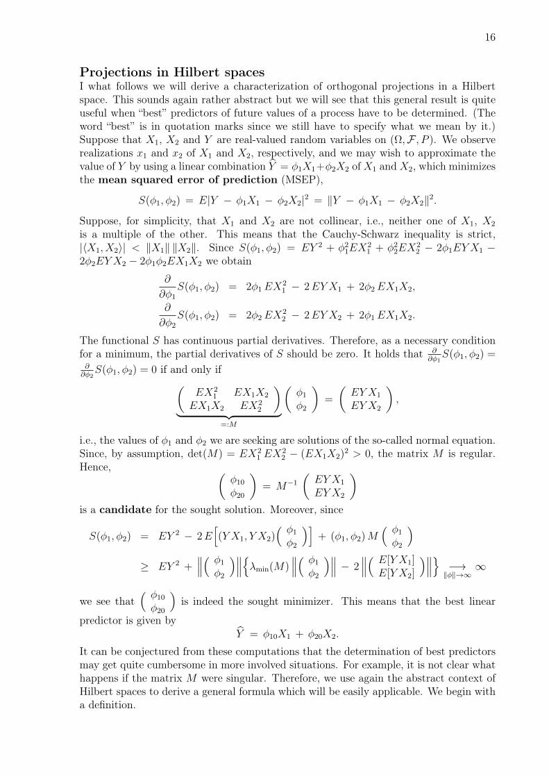
Projections in Hilbert spacesI what follows we will derive a characterization of orthogonal projections in a Hilbertspace. This sounds again rather abstract but we will see that this general result is quiteuseful when “best” predictors of future values of a process have to be determined. (Theword “best” is in quotation marks since we still have to specify what we mean by it.)Suppose that X1, X2 and Y are real-valued random variables on (Ω,F , P ). We observerealizations x1 and x2 of X1 and X2, respectively, and we may wish to approximate thevalue of Y by using a linear combination Y = φ1X1+φ2X2 ofX1 andX2, which minimizesthe mean squared error of prediction (MSEP),

S(φ1, φ2) = E|Y − φ1X1 − φ2X2|2 = ‖Y − φ1X1 − φ2X2‖2.

Suppose, for simplicity, that X1 and X2 are not collinear, i.e., neither one of X1, X2

is a multiple of the other. This means that the Cauchy-Schwarz inequality is strict,|〈X1, X2〉| < ‖X1‖ ‖X2‖. Since S(φ1, φ2) = EY 2 + φ2

1EX21 + φ2

2EX22 − 2φ1EYX1 −

2φ2EYX2 − 2φ1φ2EX1X2 we obtain

∂

∂φ1

S(φ1, φ2) = 2φ1EX21 − 2EYX1 + 2φ2EX1X2,

∂

∂φ2

S(φ1, φ2) = 2φ2EX22 − 2EYX2 + 2φ1EX1X2.

The functional S has continuous partial derivatives. Therefore, as a necessary conditionfor a minimum, the partial derivatives of S should be zero. It holds that ∂

∂φ1S(φ1, φ2) =

∂∂φ2

S(φ1, φ2) = 0 if and only if(EX2

1 EX1X2

EX1X2 EX22

)︸ ︷︷ ︸

=:M

(φ1

φ2

)=

(EYX1

EYX2

),

i.e., the values of φ1 and φ2 we are seeking are solutions of the so-called normal equation.Since, by assumption, det(M) = EX2

1 EX22 − (EX1X2)2 > 0, the matrix M is regular.

Hence, (φ10

φ20

)= M−1

(EYX1

EYX2

)is a candidate for the sought solution. Moreover, since

S(φ1, φ2) = EY 2 − 2E[(Y X1, Y X2)

( φ1

φ2

)]+ (φ1, φ2)M

( φ1

φ2

)≥ EY 2 +

∥∥∥( φ1

φ2

)∥∥∥λmin(M)∥∥∥( φ1

φ2

)∥∥∥ − 2∥∥∥( E[Y X1]

E[Y X2]

)∥∥∥ −→‖φ‖→∞

∞

we see that( φ10

φ20

)is indeed the sought minimizer. This means that the best linear

predictor is given byY = φ10X1 + φ20X2.

It can be conjectured from these computations that the determination of best predictorsmay get quite cumbersome in more involved situations. For example, it is not clear whathappens if the matrix M were singular. Therefore, we use again the abstract context ofHilbert spaces to derive a general formula which will be easily applicable. We begin witha definition.

17

Definition 1.19. A linear subspace M of a Hilbert space H is said to be a closedsubspace if M contains all of its limit points, i.e., if xn ∈ M and ‖xn − x‖ −→

n→∞0 for

some x ∈ H, then x ∈M.

Theorem 1.20. IfM is a closed subspace of the Hilbert space H and x ∈ H, then

(i) there is a unique element x ∈M such that

‖x − x‖ = infy∈M‖x − y‖,

(x is the projection of x ontoM, denoted PMx.)

(ii) x ∈M and ‖x− x‖ = infy∈M ‖x− y‖if and only if

x ∈M and 〈x− x, y〉 = 0 ∀y ∈M.

To sum up, the above theorem ensures that a projection always exists and is unique.Moreover, part (ii) provides a criterion which can be used to determine this projectionalmost effortlessly, even in complex situations. This will be illustrated by the examplegiven after the proof of this theorem.

Proof of Theorem 1.20. (i) Let d := infy∈M ‖x − y‖. Then there exists a sequence(yn)n∈N of elements ofM such that ‖x − yn‖ −→

n→∞d. We show that (yn)n∈N is a Cauchy

sequence. To this end, we use the so-called parallelogram law:

2 ‖a‖2 + 2 ‖b‖2 = ‖a+ b‖2 + ‖a− b‖2 ∀a, b ∈ H.

Then

‖ym − yn‖2 = ‖(ym − x) − (yn − x)‖2

= 2 ‖ym − x‖2 + 2 ‖yn − x‖2 − ‖(ym + yn) − 2x‖2

= 2 ‖ym − x‖2 + 2 ‖yn − x‖2 − 4 ‖ (ym + yn)/2︸ ︷︷ ︸∈M

−x‖2

≤ 2 ‖ym − x‖2 + 2 ‖yn − x‖2 − 4d2 −→m,n→∞

0.

Hence, (yn)n∈N is a Cauchy sequence and there exists an x ∈ H such that

‖yn − x‖ −→n→∞

0.

Since M is closed, x ∈ M. By continuity of the inner product (see Lemma 1.15) weobtain that

‖x − x‖2 = 〈x− x, x− x〉= lim

n→∞〈x− yn, x− yn〉

= limn→∞

‖x − yn‖2 = d2.

To establish uniqueness, suppose that x ∈M and

‖x − x‖ = ‖x − x‖ = d.

18

Then, again by the parallelogram law,

‖x − x‖2 = ‖(x− x) − (x− x)‖2

= 2 ‖x− x‖2 + 2 ‖x− x‖2 − 4 ‖(x+ x)/2 − x‖2︸ ︷︷ ︸≥d2

≤ 0,

which means that x = x.(ii) (=⇒)Suppose that x ∈ M and ‖x − x‖ = infy∈M ‖x − y‖. Suppose further that there existssome y ∈M such that

〈x− x, y〉 6= 0.

We will show that there exists some x which is closer to x than x. As a candidate, wetake x = x+ αy, where α ∈ C. (In case of a real Hilbert space, α ∈ R.) Then

‖x − x‖2 = ‖x − x − αy‖2 = 〈x − x − αy, x − x − αy〉= ‖x − x‖2 + |α|2 ‖y‖2 − α〈y, x− x〉 − α〈y, x− x〉.

Now we specify α as α = ε〈x− x, y〉, where ε ∈ R. With this choice,

‖x − x‖2 = ‖x − x‖2 + ε|〈x− x, y〉|2ε‖y‖2 − 2

< ‖x − x‖2

holds for sufficiently small ε > 0. This is a contradiction to the assumption that x is theprojection.(⇐=)Suppose that x ∈M and 〈x− x, y〉 = 0 ∀y ∈M. Let x ∈M be arbitrary. Then

‖x − x‖2 = 〈x − x + x − x, x − x + x − x〉= ‖x − x‖2 + ‖x − x‖2 + 0.

This implies that‖x − x‖ = inf

y∈M‖x− y‖.

Application: Best linear prediction of a stationary processLet X = (Xt)t∈N be a (weakly) stationary process on (Ω,F , P ) and let γX be the autoco-variance function of this process. To simplify matters we assume that EXt = 0. Supposethat realizations of X1, . . . , Xn are observed. We want to find the best linear predictorof Xn+1,

Xn+1 =n∑j=1

φj0Xn+1−j,

where

E|Xn+1 − Xn+1|2 = S(φ1, . . . , φn) := infφ1,...,φn

E∣∣∣Xn+1 −

n∑j=1

φjXn+1−j

∣∣∣2,that is, Xn+1 minimizes the mean squared error of prediction.

To determine Xn+1, we could use basic calculus as above and set the partial derivativesof the functional S equal to zero. If, in addition, the analogue of the matrix M in the

19

above example is regular, then there actually exists a unique solution. On the other hand,we could also employ the results of Theorem 1.20. This theorem tells us that a uniquesolution exists in any case, no matter if the counterpart of the matrix M is regular ornot. Moreover, it will be shown below that this solution is easily obtained using part (ii)of this theorem.

LetH = L2(Ω,F , P ) andM = ∑n

j=1 αjXn+1−j : α1, . . . , αn ∈ R. It is clear thatMis a closed linear subspace of H. Since

E(Xn+1 −

n∑j=1

φjXn+1−j

)2

=∥∥∥Xn+1 −

n∑j=1

φjXn+1−j

∥∥∥2

it follows that the sought best predictor is just the orthogonal projection of Xn+1 onto thesubspace M. Therefore we see without hesitation, that the best linear predictor existsand is unique. Part (ii) of Theorem 1.20 helps us to identify coefficients φ10, . . . , φn0

with Xn+1 =∑n

j=1 φj0Xn+1−j. These coefficients have to solve the following system ofequations:

〈Xn+1 −n∑j=1

φj0Xn+1−j, Xk〉 = 0 ∀k = n, n− 1, . . . , 1.

This is fulfilled if and only if 〈Xn+1, Xn〉...

〈Xn+1, X1〉

︸ ︷︷ ︸

=:γ

=

〈Xn+1−1, Xn〉 . . . 〈Xn+1−n, Xn〉... . . . ...

〈Xn+1−1, X1〉 . . . 〈Xn+1−n, X1〉

︸ ︷︷ ︸

=:Γn

φ10...φn0

︸ ︷︷ ︸

=:Φn

.

As already mentioned, Theorem 1.20 guarantees that there exists at least one solution,no matter whether or not the matrix Γn is regular. If γn is singular, then there existinfinitely many solutions, however, Theorem 1.20 guarantees that every solution providesthe same (uniquely defined) predictor Xn+1.

Exercise

Ex. 1.4 Suppose that Y and Z are uncorrelated random variables with EY = EZ = 0 andEY 2 = EZ2 = 1. For t ∈ N, let Xt = Y cos(θt) + Z sin(θt), where θ ∈ R.

Show that X3 = 2 cos(θ)X2 −X1 is the best linear predictor of X3 given X1, X2.

Hint: E[XsXt] = cos(θ(s− t)) and cos(2θ) = (cos(θ))2 − (sin(θ))2.

20

1.3 Linear processes

In this section, we consider so-called linear processes. Their simple structure allows us toderive their properties without much effort. Even a counterpart to the Lindeberg-Lévycentral limit theorem can be easily derived. Moreover, it will be shown in the followingsection that certain processes with a more involved structure can be represented as sucha linear process. We begin with a few definitions.

Definition 1.21. The process ε = (εt)t∈Z is said to be white noise if

Eεt = 0 ∀t, cov(εt+h, εt) =

σ2ε if h = 0

0 if h 6= 0.

Notation: (εt)t∈Z ∼WN(0, σ2ε).

If (εt)t∈Z is a sequence of independent and identically distributed random variables withEεt = 0 and var(εt) = σ2

ε , then

(εt)t∈Z ∼ IID(0, σ2ε).

Definition 1.22. Let (εt)t∈Z be a real-valued process on (Ω,F , P ). Then the processX = (Xt)t∈Z defined by

Xt =∞∑

k=−∞

βkεt−k

is said to be a linear process. In this context, the εt are called innovations.

Special cases:

• Xt =∑q

k=0 βkεt−kThen (Xt)t∈Z is an MA(q) process (moving average process of order q).

• Xt =∑∞

k=0 βkεt−kThen (Xt)t∈Z is an MA(∞) process. (causal linear process)

Remark 1.23. Regarding the sequence of innovations, there are different definitionsof linear processes in the literature. For example, Brockwell and Davis (“Time Series:Theory and Methods”) suppose that (εt)t∈Z ∼ WN(0, σ2

ε) whereas Kreiß and Neuhaus(“Einführung in die Zeitreihenanalyse”) assume that (εt)t∈Z ∼ IID(0, σ2

ε). In what follows,we adapt our assumption on the innovation process to the respective purpose.

Note that the definition of a linear process involves an infinite series and it is not clearwhether or not this series converges. The following proposition provides sufficient condi-tions for their convergence.

21

Proposition 1.24. Let (εt)t∈Z be a sequence of real-valued random variables on (Ω,F , P )and (βk)k∈Z be an absolutely convergent series (i.e.

∑∞k=−∞ |βk| <∞).

(i) If suptE|εt| <∞, then the series

Xt =∞∑

k=−∞

βkεt−k

converges absolutely with probability 1.

(ii) If suptE[ε2t ] <∞, then the series converges in mean square to the same limit, i.e.,

Xt,m :=m∑

k=−m

βkεt−kL2

−→ Xt.

Proof. (i) The monotone convergence theorem yields that

E[ ∞∑k=−∞

|βkεt−k|]

= limn→∞

E[ n∑k=−n

|βk| |εt−k|]

= limn→∞

n∑k=−n

|βk|E|εt−k|

≤(

limn→∞

n∑k=−n

|βk|)

suptE|εt| < ∞.

Therefore,

P( ∞∑k=−∞

|βkεt−k| <∞)

= 1,

that is, the series∑∞

k=−∞ βkεt−k converges absolutely with probability 1. We denote thelimit by Xt.(ii) Let Xt,m :=

∑mk=−m βkεt−k. Then, for m < n,

‖Xt,n − Xt,m‖2 = 〈∑

m<|j|≤n

βjεt−j,∑

m<|k|≤n

βkεt−k〉

=∑

m<|j|≤n

∑m<|k|≤n

βjβkE[εt−jεt−k]

≤( ∑m<|j|≤n

|βj|)2

︸ ︷︷ ︸→0 as m,n→∞

suptE[ε2

t ].

Therefore,‖Xt,n − Xt,m‖ −→ 0 as m,n→∞,

i.e., (Xt,m)m∈N is a Cauchy sequence in L2(Ω,F , P ). It follows from Theorem 1.18 (com-pleteness of L2(Ω,F , P )) that there exists some Xt ∈ L2(Ω,F , P ) such that

‖Xt,m − Xt‖ −→m→∞

0.

22

Furthermore, we obtain by Fatou’s lemma that

E[|Xt − Xt|2

]= E

[lim infm→∞

|Xt − Xt,m|2]

≤ lim infm→∞

E[|Xt − Xt,m|2

]= 0,

which implies thatP(Xt = Xt

)= 1.

Exercise

Ex. 1.5 Let (εt)t∈Z ∼WN(0, σ2ε) and Xt =

∑∞k=0 α

kεt−k, for some α ∈ R, |α| < 1.

Show that Xn+1 := αXn is the best linear predictor of Xn+1 given X1, . . . , Xn.

1.4 Autoregressive processes

1.5 ARMA processes

2 Spectral analysis of stationary processes

2.1 Spectral density, spectral distribution function

2.2 Estimation in the spectral domain