Lecture Notes on the Optimizer’s Curse - Technion

OPTIMIZER’S CURSE 1

Lecture Notes on the Optimizer’s CurseYakov Ben-Haim

Yitzhak Moda’i Chair in Technology and EconomicsFaculty of Mechanical Engineering

Technion — Israel Institute of TechnologyHaifa 32000 Israel

[email protected]://info-gap.com http://www.technion.ac.il/yakov

A Note to the Student: These lecture notes are not a substitute for the thorough study ofarticles and books. These notes are no more than an aid in following the lectures.

§ Sources:• Smith, James E. and Robert L. Winkler, 2006, The optimizer’s curse: Skepticism and

postdecision surprise in decision analysis, Management Science, Vol. 52, No. 3, pp.311–322.• Thaler, Richard H., 1992, The Winner’s Curse: Paradoxes and Anomalies of Economic

Life, Princeton University Press.

Contents1 Probabilistic Analysis 2

1.1 Formulation . . . . . . . . . . . . . . . . . . . . . . . . . . . . . . . . . . . . . . . . . . 21.2 Simple Examples . . . . . . . . . . . . . . . . . . . . . . . . . . . . . . . . . . . . . . . 3

1.2.1 3 Zero-Mean Alternatives . . . . . . . . . . . . . . . . . . . . . . . . . . . . . . 31.2.2 n Zero-Mean Alternatives . . . . . . . . . . . . . . . . . . . . . . . . . . . . . . 41.2.3 3 Different Alternatives . . . . . . . . . . . . . . . . . . . . . . . . . . . . . . . . 5

1.3 Distribution of vi? . . . . . . . . . . . . . . . . . . . . . . . . . . . . . . . . . . . . . . . 61.4 Optimizer’s Curse Theorem . . . . . . . . . . . . . . . . . . . . . . . . . . . . . . . . . 8

2 Info-Gap Analysis 92.1 Robustness: Formulation . . . . . . . . . . . . . . . . . . . . . . . . . . . . . . . . . . 92.2 Robustness: Simple Example . . . . . . . . . . . . . . . . . . . . . . . . . . . . . . . . 102.3 Probability of Success and the Proxy Property . . . . . . . . . . . . . . . . . . . . . . 112.4 Proxy Property: Simple Examples . . . . . . . . . . . . . . . . . . . . . . . . . . . . . 12

2.4.1 Normal Distribution . . . . . . . . . . . . . . . . . . . . . . . . . . . . . . . . . . 122.4.2 Uniform Distribution . . . . . . . . . . . . . . . . . . . . . . . . . . . . . . . . . 12

2.5 Standardization and the Proxy Property . . . . . . . . . . . . . . . . . . . . . . . . . . 142.6 Coherence . . . . . . . . . . . . . . . . . . . . . . . . . . . . . . . . . . . . . . . . . . 162.7 Coherence and the Proxy Property . . . . . . . . . . . . . . . . . . . . . . . . . . . . . 18

0lectures\info-gap-methods\lectures\optimizers-curse04.tex 24.12.2019 c© Yakov Ben-Haim 2019.

\info-gap-methods\lectures\optimizers-curse04.tex OPTIMIZER’S CURSE 2

1 Probabilistic Analysis

1.1 Formulation

§ n alternatives: 1, . . . , n.• vi = Unknown true value of ith alternative. v = (v1, . . . , vn)T .• vi = Known noisy estimated value of ith alternative. v = (v1, . . . , vn)T .

§ Regret:• Choose alternative i, expecting vi.• Obtain realized outcome vi.• Regret, or disappointment: vi − vi.

Positive regret if vi < vi.

§ Unbiased estimates:E(vi|v) = vi (1)

Thus, for any choice i, the expected regret is zero:

E(vi − vi|v) = 0 (2)

This is because:E(vi|v) = vi = E(vi|v) (3)

§ Outcome optimization:i? = arg max

ivi (4)

§ Question: Is this a good, sensible strategy?

§ Expect positive regret from vi?.• Example:◦ Suppose E(vi) = µ, a constant, for all i.◦ Anticipate E(vi?) > µ since:

– vi? is the maximum of n estimates.– vi? will tend to be on upper tail. (Example: best grade of n exams.)

◦ Hence E(vi? − vi?) = E(vi?)− µ > 0.• Meaning: On average, estimated outcome optimum:◦ Is over-estimate.◦ Has positive regret.

•We will explore this more deeply later.


1.2 Simple Examples

§We consider some simple examples from Smith and Winkler (2006).

1.2.1 3 Zero-Mean Alternatives

§ The true values, vi, all precisely equal zero. They are not random variables.

§ The estimates, vi, are all N (0, 1). See fig. 1.

312Smith and Winkler: The Optimizer's Curse: Skepticism and Postdecision Surprise in Decision Analysis

Management Science 52(3), pp. 311-322, ©2006 INFORMS

doing, may affect the recommendations derived fromthe analysis. The prescription calls for treating thedecision-analysis-based value estimates like the noisyestimates that they are and mixing them with priorestimates of value, in essence treating the decision-analysis-based value estimates somewhat skeptically.In §4, we discuss related biases, including the win-ner's curse, and in §5, we offer some concludingcomments.

2. The Optimizer's CurseSuppose that a decision m aker is considering n alter-natives whose true values are denoted fi-i,..., (£„.We can think of these "true values" as represent-ing the expected value or expected utility (whicheveris the focus of the analysis) that would be foundif we had unlimited resources—time, money, com-putational capabilities—at our disposal to conductthe analysis. A decision analysis study produces esti-mates Vj , , . . , Vj, of the values of these alternatives.These estimates might be the result of, say, a $50,000consulting effort, whereas it might cost millions to cal-culate the true value to the decision maker.

The standard decision analysis process ranks alter-natives by their value estimates and recommendschoosing the alternative i* that has the highest esti-mated value Vj.. Under uncertainty, the true value i,.of a recommended alternative is typically neverrevealed. We can, however, view the realized value Xj,as a random draw from a distribution with expectedvalue )u.,. and, following Harrison and March (1984),think of the difference x,. - V,. between the realizedvalue and value estimate as the postdecision surpriseexperienced by the decision maker. A positive sur-prise represents some degree of elation and a neg-ative surprise represents disappointment. Averagingacross many decisions, the average postdecision sur-prise Xj. — V,. will tend toward the average expectedsurprise, E[/i,,. - V .].

If the value estimates produced by a decisionanalysis are conditionally unbiased in that E[V,|/AJ,. . . , l„] = /Xi for all i, then the estimated value of anyalternative should lead to zero expected surprise, i.e.,E[/x, — V,] = 0. However, if we consistently choose thealternative with highest estimated value, this selectionprocess leads to a negative expected surprise, even if

' Our use of "true values" is in the spirit of Matheson (1968), whorefers to probabilities or values "given by a complete analysis." Tani(1978) objects to the use of "true" in this context, noting that thisvalue is subjective and depends on the decision maker's state ofinformation; he refers to "authentic probabilities" rather than "trueprobabilities." These concerns notwithstanding, the use of the term"true values" in this setting seems both natural and standard, hav-ing been used by Lindley et al. (1979) and Lindley (1986), amongothers.

the value estimates are conditionally unbiased. Thus,a decision maker who consistently chooses alterna-tives based on her estimated values should expect tobe disappointed on average, even if the individualvalue estimates are conditionally unbiased. We for-malize this optimizer's curse in §2.3 after illustratingit with some examples.

2.1. Some Prototypical ExamplesTo illustrate the optimizer's curse in a simple set-ting, suppose that we evaluate three alternatives thatall have true values (/A,) of exactly zero. The valueof each alternative is estimated and the estimates V,are independent and normally distributed with meanequal to the true value of zero (they are conditionallyunbiased) and a standard deviation of one. Selectingthe highest value estimate then amounts to selectingthe maximum of three draws from a standard normaldistribution. The distribution of this maximal valueestimate is easily determined by simulation or usingresults from order statistics and is displayed in Fig-ure 1. The mean of this distribution is 0.85, so in thiscase, the expected disappointment, E[Vj. - JLI,.], is 0.85.Because the results of this example are scale and loca-tion invariant, we can conclude that given three alter-natives with identical true values and independent,identical, and normally distributed unbiased valueestimates, the expected disappointment will be 85%of the standard deviation of the value estimates.

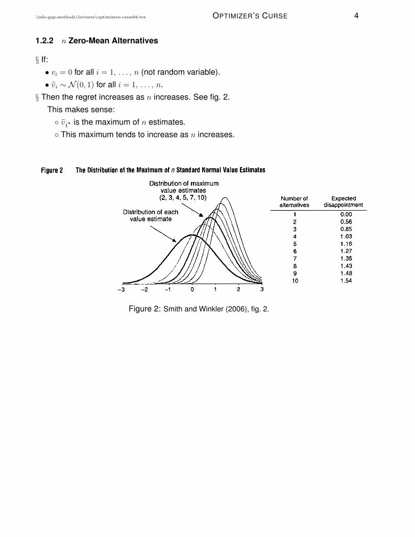
This expected disappointment increases with thenumber of alternatives considered. Continuing withthe same distribution assumptions and varying thenumber of alternatives considered, we find the resultsshown in Figure 2. Here, we see that the distributionsshift to the right as we increase the number of alter-natives and the means increase at a diminishing rate.With four alternatives, the expected disappointmentreaches 103% of the standard deviation of the valueestimates, and with 10 it reaches 154% of the standarddeviation of the value estimates.

Figure 1 The Distribution of the iViaximum of Three Standard NormalVaiue Estimates

Distribution of eachvalue estimate

(EV = 0)

Distribution of maximumvalue estimate

(EV = 0.85)

Figure 1: Smith and Winkler (2006), fig. 1.

§ The mean of the distribution of vi? is 0.85.(We will understand this more deeply later.)

§ Thus the average regret, E(vi? − 0), is 0.85.

§ More generally, suppose:• The true values are vi = µ for all i. They are not random variables.• The estimates, vi, are all N (µ, σ2).• Then E(vi?) = µ+ 0.85σ which is the average regret.


1.2.2 n Zero-Mean Alternatives

§ If:• vi = 0 for all i = 1, . . . , n (not random variable).• vi ∼ N (0, 1) for all i = 1, . . . , n.

§ Then the regret increases as n increases. See fig. 2.This makes sense:◦ vi? is the maximum of n estimates.◦ This maximum tends to increase as n increases.

Smith and Winkler: The Optimizer's Curse: Skepticism and Postdecision Surprise in Decision AnalysisManagement Science 52(3), pp. 311-322, ©2006 INFORMS 313

Figure 2 The Distribution of the iVIaxImum of n Standard Normai Value Estimates

Distribution of maximumvaiue estimates(2,3,4,5,7,10)


Number ofalternatives

12345678910

Expecteddisappointment

0.000.560.851.031.161.271.351.431.481.54

The case where the true values are equal is, in asense, the worst possible case because the alterna-tives cannot be distinguished even with perfect valueestimates. Figure 3 shows the results in the case ofthree alternatives, where the true values are separatedby A: t, = -A, 0, -|-A. The value estimates are againassumed to be unbiased with a standard deviationof one. In Figure 3, we see that the magnitude ofthe expected disappointment decreases with increas-ing separation. Intuitively, the greater the separationbetween the alternative that is truly the best and theother alternatives, the more likely it is that we willselect the correct alternative. If we always select thetruly optimal alternative, then the expected disap-pointment would be zero because its value estimateis unbiased.

We have assumed that the value estimates are inde-pendent in the above examples. In practice, how-ever, the value estimates may be correlated, as thevalue estimates for different alternatives may sharecommon elements. For example, in a study of differ-ent strategies to develop an R&D project, the valueestimates may all share a common probability fortechnical success; errors in the estimate of this proba-bility would have an impact on the values of all of the

alternatives considered. Similarly, a study of alterna-tive ways to develop an oil field may share a commonestimate (or probability distribution) of the amount ofoil in place. In practice then, we might expect valueestimates to be positively correlated.

To illustrate the impact of correlation in value esti-mates, consider a simple discrete example with twoalternatives that have equal true values and valueestimates that are equally likely to be low or highby some fixed amount. This setup is illustrated inTable 1. If the two value estimates are independent,there is a 75% chance that we will observe a highvalue estimate for at least one alternative and over-estimate the true value of the optimal alternative anda 25% chance of underestimating the true value; thevalue estimate of the selected alternative wiU thusoverestimate the true value on average. If the twovalue estimates are perfectly positively correlated,there is a 50% chance of both estimates being highand a 50% chance of both being low, and we wouldhave an estimate for the selected alternative that isequal to the true value on average. Thus, we shouldexpect positive correlation to decrease the magni-tude of the expected disappointment. Negative cor-relation, on the other hand, should increase expected

Figure 3 The Distribution of iVIaximum Vaiue Estimates with Separation Between Aiternatives

Distribution of maximum value estimate

Distribution of vaiueestimates(A = 0.5)

A

0.00.20.40.60.81.01.21.41.61.82.02.22.42.62.83.0


0.850.660.510.390.300.220.170.120.100.070.050.030.020.010.010.00

Probability ofcorrect ctioice

0.330.420.500.590.660.730.780.830.870.900.920.940.950.970.980.98



1.2.3 3 Different Alternatives

§ The true values are vi = −∆, 0, ∆. Not random variables.

§ The estimates are unbiased normal with unit standard deviation: vi ∼ N (vi, 1).

§ As the alternatives become more different, we should expect vi? to become a better bet.See fig. 3.

Smith and Winkler: The Optimizer's Curse: Skepticism and Postdecision Surprise in Decision AnalysisManagement Science 52(3), pp. 311-322, ©2006 INFORMS 313

Figure 2 The Distribution of the iVIaxImum of n Standard Normai Value Estimates

Distribution of maximumvaiue estimates(2,3,4,5,7,10)


Number ofalternatives

12345678910


0.000.560.851.031.161.271.351.431.481.54

The case where the true values are equal is, in asense, the worst possible case because the alterna-tives cannot be distinguished even with perfect valueestimates. Figure 3 shows the results in the case ofthree alternatives, where the true values are separatedby A: t, = -A, 0, -|-A. The value estimates are againassumed to be unbiased with a standard deviationof one. In Figure 3, we see that the magnitude ofthe expected disappointment decreases with increas-ing separation. Intuitively, the greater the separationbetween the alternative that is truly the best and theother alternatives, the more likely it is that we willselect the correct alternative. If we always select thetruly optimal alternative, then the expected disap-pointment would be zero because its value estimateis unbiased.

We have assumed that the value estimates are inde-pendent in the above examples. In practice, how-ever, the value estimates may be correlated, as thevalue estimates for different alternatives may sharecommon elements. For example, in a study of differ-ent strategies to develop an R&D project, the valueestimates may all share a common probability fortechnical success; errors in the estimate of this proba-bility would have an impact on the values of all of the

alternatives considered. Similarly, a study of alterna-tive ways to develop an oil field may share a commonestimate (or probability distribution) of the amount ofoil in place. In practice then, we might expect valueestimates to be positively correlated.

To illustrate the impact of correlation in value esti-mates, consider a simple discrete example with twoalternatives that have equal true values and valueestimates that are equally likely to be low or highby some fixed amount. This setup is illustrated inTable 1. If the two value estimates are independent,there is a 75% chance that we will observe a highvalue estimate for at least one alternative and over-estimate the true value of the optimal alternative anda 25% chance of underestimating the true value; thevalue estimate of the selected alternative wiU thusoverestimate the true value on average. If the twovalue estimates are perfectly positively correlated,there is a 50% chance of both estimates being highand a 50% chance of both being low, and we wouldhave an estimate for the selected alternative that isequal to the true value on average. Thus, we shouldexpect positive correlation to decrease the magni-tude of the expected disappointment. Negative cor-relation, on the other hand, should increase expected

Figure 3 The Distribution of iVIaximum Vaiue Estimates with Separation Between Aiternatives

Distribution of maximum value estimate

Distribution of vaiueestimates(A = 0.5)

A

0.00.20.40.60.81.01.21.41.61.82.02.22.42.62.83.0


0.850.660.510.390.300.220.170.120.100.070.050.030.020.010.010.00

Probability ofcorrect ctioice

0.330.420.500.590.660.730.780.830.870.900.920.940.950.970.980.98



1.3 Distribution of vi?

§ In this section we derive and study the distribution of vi?.•We will understand why its mean exceeds E(vi).• Source: DeGroot, Morris H., 1986, Probability and Statistics, 2nd ed., Addison-Wesley,

Reading, MA. Section 3.2, pp.182–183.

§ vi is the estimated value of the ith alternative.• Its cumulative probability distribution (cpd) is Fi(v).• All the vi are statistically independent.

§ vi? = maxi vi.Its cpd is G(v), derived as follows:

G(v) = Prob(vi? ≤ v) (5)

= Prob(v1 ≤ v, . . . , vn ≤ v) (6)

=n∏i=1

Fi(v) (7)

§ If the vi are i.i.d. with cpd F (v) and pdf f(v) then:

G(v) = [F (v)]n (8)

g(v) =∂G

∂v= n[F (v)]n−1f(v), where f(v) =

∂F

∂v(9)

§ Now compare E(vi?) and E(vi) for i.i.d. case:

E(vi?) =∫vg(v) dv (10)

=∫vn[F (v)]n−1f(v) dv (11)

E(vi) =∫vf(v) dv (12)

Thus:

E(vi?)− E(vi) =∫v[g(v)− f(v)] dv =

∫vf(v)

(n[F (v)]n−1 − 1

)dv (13)

This integral is positive for n ≥ 2, as we now explain intuitively.


-

6

f(v) g(v)

0 vv(1)

Figure 4: Illustration of yn.

§ Define v(1) as the value at which: n[F (v(1))]n−1 = 1. This is also the value at whichf(v) = g(v). See fig. 4.• Hence: F (v(1)) = (1/n)1/(n−1).• Note that n[F (v)]n−1 ≤ 1 iff v ≤ v(1) because F (v) increases monotonically in v.• Hence, from eq.(9), note that g(y) ≤ f(v) for v ≤ v(1) as seen in fig. 4.• Thus, since g(v) is normalized, it is shifted to the right wrt f(v).• Thus, E(vi?) ≥ E(vi).


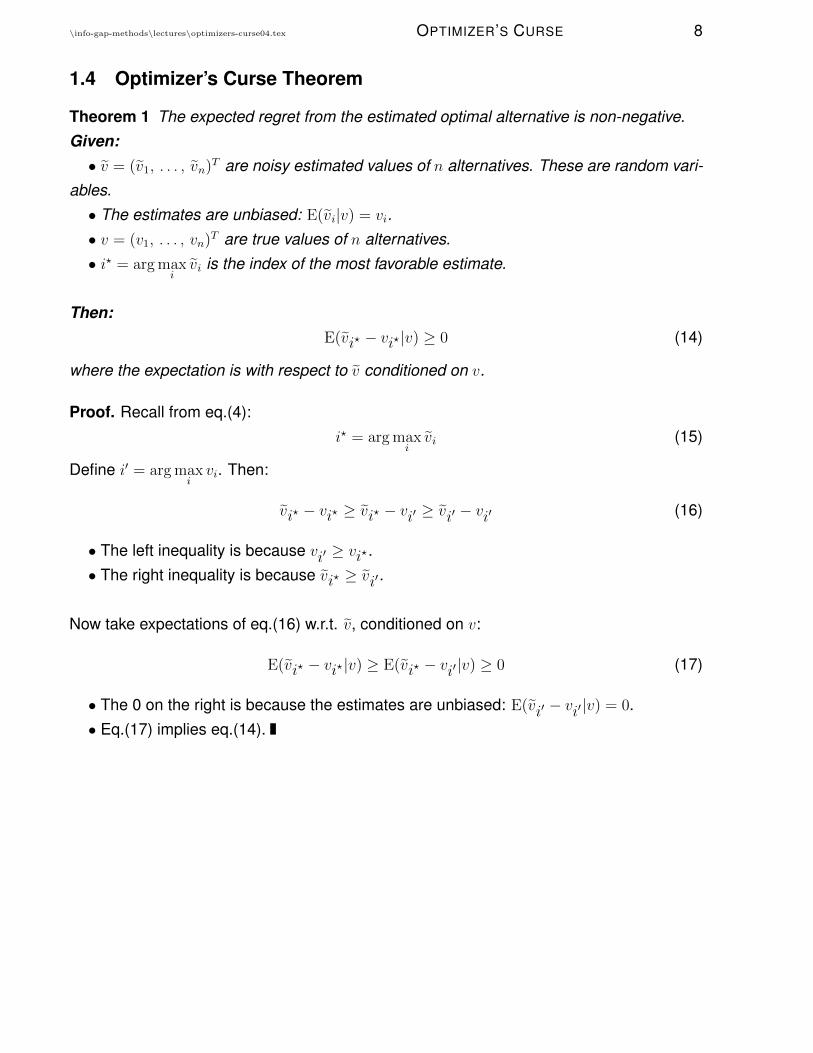
1.4 Optimizer’s Curse Theorem

Theorem 1 The expected regret from the estimated optimal alternative is non-negative.Given:• v = (v1, . . . , vn)T are noisy estimated values of n alternatives. These are random vari-

ables.• The estimates are unbiased: E(vi|v) = vi.• v = (v1, . . . , vn)T are true values of n alternatives.• i? = arg max

ivi is the index of the most favorable estimate.

Then:E(vi? − vi?|v) ≥ 0 (14)

where the expectation is with respect to v conditioned on v.

Proof. Recall from eq.(4):i? = arg max

ivi (15)

Define i′ = arg maxivi. Then:

vi? − vi? ≥ vi? − vi′ ≥ vi′ − vi′ (16)

• The left inequality is because vi′ ≥ vi?.• The right inequality is because vi? ≥ vi′.

Now take expectations of eq.(16) w.r.t. v, conditioned on v:

E(vi? − vi?|v) ≥ E(vi? − vi′ |v) ≥ 0 (17)

• The 0 on the right is because the estimates are unbiased: E(vi′ − vi′|v) = 0.• Eq.(17) implies eq.(14).


2 Info-Gap Analysis

§ Related material in “Lecture Notes on Robust-Satisficing Behavior”, section 6: Probabilityof Success. File: lectures\info-gap-methods\lectures\rsb02.tex.

§ Question: Since vi? is unreliable (it has positive regret), what should we do?

§ A Potential answer. Bayesian analysis (Smith and Winkler, 2006):• Posit prior probability for v, p(v), and conditional probability for v given v, p(v|v).• Use Bayes’ rule to determine posterior probability of v given v: p(v|v).• Choose alternative based on posterior means, E(vi|v):

i? = arg maxi

E(vi|v) (18)

• Smith and Winkler (2006) show that this solution does not have the optimizer’s curse!• The problem: where do you get these pdf’s?

§ A potential answer. Info-gap robust-satisficing:• Satisfice the value: vi ≥ vc. (We will find the regret entering later.)• Maximize the robustness.

§ A potential answer. Info-gap opportune-windfalling:•Windfall the value: vi ≥ vw where vw � vc.• Maximize the opportuneness.

§We will explore:• Robust-satisficing.• Proxy theorems.

2.1 Robustness: Formulation

§ Observations: known noisy estimated values of n alternatives: v = (v1, . . . , vn)T .

§ Uncertainty:• Unknown true values of n alternatives: v = (v1, . . . , vn)T .• V(h) = info-gap model for v. E.g.:

V(h) ={v :

∣∣∣∣vi − visi

∣∣∣∣ ≤ h, ∀i}, h ≥ 0 (19)

Or:V(h) =

{v : (v − v)TS−1(v − v) ≤ h2

}, h ≥ 0 (20)


§ Decision: r is the decision vector. E.g.:• A standard unit basis vector, selecting a single alternative.• An n-vector probability distribution selecting a randomized mix of alternatives.

§ Performance function. Value:q(r, v) = rTv (21)

§ Performance requirement. Satisfice the value:

q(r, v) ≥ qc (22)

§ Robustness:

h(r, qc) = max

{h :

(minv∈V(h)

rTv

)≥ qc

}(23)

2.2 Robustness: Simple Example

§We evaluate the robustness, eq.(23), with the info-gap model of eq.(19).

§ Let µ(h) denote the inner minimum in eq.(23).• µ(h) occurs when rTv is minimal.• The elements of r are non-negative, so µ(h) occurs when each vi is minimal:

µ(h) =n∑i=1

(vi − sih)ri (24)

= rT v − hrT s (25)

Equating this to qc and solving for h yields the robustness:

h(r, qc) =rT v − qcrT s

(26)

or zero if this is negative.

§ Regret. The numerator in eq.(26) is a regret:• rT v: expected outcome.• qc: required or critical or least acceptable outcome.• Positive regret: critical outcome lower than expectation: rT v − qc > 0.• Zero regret has zero robustness. This is related to the zeroing property.• Positive regret has positive robustness.

This is related to the trade off of robustness vs. performance.§ Preference reversal. It is evident from eq.(26) that robustness curves of different deci-sions can cross one another.


2.3 Probability of Success and the Proxy Property

1

§ Probability of success:• Define q = rTv.• Q(h) = info-gap model for uncertainty in q.• Requirement: q ≥ qc.• p(q|r) = pdf of q given r. This pdf is unknown.• Ps(r, qc) = probability of satisfying the requirement with r:

Ps(r, qc) = Prob(q ≥ qc) =∫ ∞qc

p(q|r) dq (27)

§ Probabilistic preferences:

r1 �p r2 if Ps(r1, qc) > Ps(r2, qc) (28)

§ Robust-satisficing preferences:

r1 �r r2 if h(r1, qc) > h(r2, qc) (29)

§ Proxy Property:

Definition 1 Qr(h) and P (q|r) have the proxy property at decisions r1 and r2 and criticalvalue qc, with performance function G(r, q), if:

h(r1, qc) > h(r2, qc) if and only if Ps(r1, qc) > Ps(r2, qc) (30)

• The proxy property is symmetric between robustness and probability of success.•We are particularly interested in the implication from robustness to probability.• Thus, when the proxy property holds we will sometimes say that robustness is a proxy

for probability of success.• Sounds like a free lunch!

§ Proxy theorem: The proxy property holds if and only if the info-gap model and theprobability distribution are “coherent”. We will return to the idea of coherence in section 2.6.

1Significant overlap between sections 2.3–2.6 here and section 6 in Lecture Notes on Robust-SatisficingBehavior, rsb02.tex.


2.4 Proxy Property: Simple Examples

§ Before discussing coherence we examine simple examples of the proxy property, basedon the simple example in section 2.2.

2.4.1 Normal Distribution

§ Let q = rTv be normal:q ∼ N

[rT v, (rT s)2c2

](31)

where c > 0.

§ The probability of success, eq.(27), is:

Ps(r, qc) = Prob(q ≥ qc) (32)

= Prob

(q − rT v(rT s)c

≥ qc − rT v(rT s)c

)(33)

= 1− Φ

(qc − rT v(rT s)c

)(34)

= 1− Φ

(− h(r, qc)

c

)(35)

where eq.(35) results from eq.(26). Φ(·) is the cpd of the standard normal variable.

§ Proxy property holds.• From eq.(35) we see that Ps(r, qc) depends on r only through h(r, qc).• Hence eq.(35) implies eq.(30) and the proxy property holds.•We only need to know that:◦ q is normal with mean rT v.◦ That c > 0. We needn’t know the variance.

2.4.2 Uniform Distribution

§ Define uniform distributions as:

p(y|a, b) =

1b− a if a ≤ y ≤ b

0 else(36)

§ Suppose q = rTv is uniform, p(q|a, b), where:

a = rT v − c

2rT s (37)

b = rT v +c

2rT s (38)


where c > 0.

§ Probability of success, as in eqs.(32) and (33), is:

Ps(r, qc) = Prob(q ≥ qc) (39)

= Prob

(q − rT v(rT s)c

≥ qc − rT v(rT s)c

)(40)

§ Define:

z =q − rT v(rT s)c

(41)

which is uniform, p(z|a, b), with:

a = − c2

(42)

b =c

2(43)

§ Now probability of success is analogous to eqs.(34) and (35):

Ps(r, qc) = Prob

(z ≥ qc − rT v

(rT s)c

)(44)

= 1− P(qc − rT v(rT s)c

|a, b)

(45)

= 1− P(− h(r, qc)

c|a, b

)(46)

where a and b are independent of r, eqs.(42) and (43).

§ Proxy property holds.• From eq.(46) we see that Ps(r, qc) depends on r only through h(r, qc).• Hence eq.(46) implies eq.(30) and the proxy property holds.•We only need to know that:◦ q is uniform with mean rT v.◦ That c > 0. We needn’t know the variance.


2.5 Standardization and the Proxy Property

§ Probability of survival.• Option i succeeds (survives) if its value is no less than the critical value:

vi ≥ vc (47)

• Fi(·) denotes the cumulative probability distribution function of vi.• Probability of success for option i is:

Ps(i) = Prob(vi ≥ vc) = 1− Fi(vc) (48)

§ Standardization class of probability distributions:

Definition 2 Let q be a scalar random variable with a pdf that depends on parameters r.The pdf is standardizable and θ(q, r) is a standardization function if θ(q, r) is a scalarfunction which is strictly increasing and continuous in q at any fixed r and whose pdf is thesame for all r.

§ Example:• f(q|r) is a pdf of a random variable q, where r is a vector of parameters of the pdf.• f(q|r) is a class of pdfs parametrized by r.• Mean and variance of q are µq and σ2

q . E.g. r = (µq, σ2q ).

• Standardized random variable, with pdf g(θ), is:

θ = (q − µq)/σq (49)

• If g(θ) is independent of r then this is a standardization class. That is, if all the stan-dardized random variables in the class have the same pdf, then this is a standardizationclass.• Standardization classes are quite common:◦ the normal, uniform, and exponential distributions all being examples.◦ The standardized distribution g(θ) may belong to the standardization class, e.g. nor-

mal and uniform, but this is not necessarily true, e.g. the exponential.

¶ Example: exponential distribution:

f(q|r) = re−rq, q ≥ 0 (50)

Moments:E(q|r) = σ(q|r) =

1

r(51)

Standardized variable:θ =

q − E(q|r)σ(q|r)

= rq − 1 (52)


Standardized density by probability balance:

q =θ + 1

r, dq =

1

rdθ =⇒ g(θ)dθ = f(q|r)dq = e−rqrdq = e−(θ+1)dθ, θ ≥ −1 (53)

Standardized density and cumulative distribution:

g(θ) = e−(θ+1), θ ≥ −1, G(θ) =∫ θ

−1g(z) dz = 1− e−(θ+1) (54)

g(θ) is a shifted exponential distribution.

¶ Proxy property: example.• Suppose vi and vj both belong to the same standardization class.• Their info-gap model is eq.(19), p.9, and robustness is eq.(26), p.10.• Their standardization functions are:

θ(vi) =vi − vicsi

(55)

where c > 0.• G(θ) = cumulative probability distribution function of the standardized random vari-

ables.• Probability of success for option i is:

Ps(i) = Prob(vi ≥ vc) = Prob(vi − vicsi

≥ vc − vicsi

)(56)

= 1−G(vc − vicsi

)(57)

= 1−G[− h(i, vc)

c

](58)

where eq.(58) results from eqs.(57) and (26) if vc ≤ vi.•We see that:

Ps(i) > Ps(j) if and only if h(i, vc) > h(j, vc) (59)

• This example illustrates a general result:Standardization implies that the proxy property holds.• In order to calculate h(i, vc) and hence maximize Ps(i) we must be able to standardize

the vi’s, eq.(55).• This requires knowing, for each i:◦ vi = mean.◦ csi proportional to standard deviation.

• This does not require knowing:◦ Value of c (actual standard deviations).◦ Identify of pdf.


2.6 Coherence

§ Coherence:• A weak informational-overlap between an info-gap model and a probability distribution.• Coherence is necessary and sufficient for the proxy property to hold.

§ Scalar uncertainty, q.• r is the decision vector.• E.g. q = rTv.• Qr(h) is info-gap model for q.• P (q|r) and p(q|r) are cumulative prob distribution (cpd) and pdf for q.• G(r, q) is the performance function. Monotonic in q.• Define:

q?(h, r) ≡ maxq∈Qr(h)

q (60)

q?(h, r) ≡ minq∈Qr(h)

q (61)

µ(h) ≡ minq∈Qr(h)

G(r, q) (62)

• Define inverse of G(r, q), at fixed r, as follows.If G(r, q) increases as q increases:

G−1(r, qc) ≡ max {q : G(r, q) ≤ qc} (63)

If G(r, q) decreases as q increases:

G−1(r, qc) ≡ min {q : G(r, q) ≤ qc} (64)

Definition 3 . Qr(h) and P (q|r) are upper coherent at decisions r1 and r2 and criticalvalue qc, with performance function G(r, q), if the following two relations hold for i = 1 ori = 2, and j = 3− i:

P [G−1(ri, qc)|ri] > P [G−1(rj, qc)|rj] (65)

G−1(ri, qc)− q?(h, ri) > G−1(rj, qc)− q?(h, rj)

for h = h(rj, qc) and h = h(ri, qc) (66)

Qr(h) and P (q|r) are lower coherent if eqs.(65) and (66) hold when q?(h, r) is replaced byq?(h, r).

• Coherence implies “information overlap” between Qr(h) and P (q|r).• Eq.(65) depends on P (q|r) but not on h or Qr(h).• Eq.(66) depends on h and Qr(h) but not on P (q|r).


• Coherence implies that knowledge of one function reveals something about the other.

§ Example. Following are coherent with G(r, q) = q/r:

P (q|r) = 1− e−rq (67)

Qr(h) =

{q : 0 ≤ q ≤ h

r

}, h ≥ 0 (68)

• As r increases, P (q|r) and Qr(h) both become more highly concentrated.• Each reveals something about the other. There is some “coherence” between them.

§ Example. Following are not coherent withG(r, q) = q/r: Exponential distribution, eq.(67),and:

Qr(h) = {q : 0 ≤ q ≤ rh} , h ≥ 0 (69)

• As r increases, P (q|r) becomes more highly focussed while Qr(h) becomes more dis-persed.


2.7 Coherence and the Proxy Property

§We now state and discuss an important theorem:coherence is necessary and sufficient for the proxy property to hold.

Definition 4 An info-gap model, Qr(h), expands upward continuously at h if, for anyε > 0, there is a δ > 0 such that:

|q?(h′, r)− q?(h, r)| < ε if |h′ − h| < δ (70)

Continuous downward expansion is defined similarly with q?(·) instead of q?(·).

We can now state a proposition.2

Proposition 1 Info-gap robustness to an uncertain scalar variable, with a loss functionwhich is monotonic in the uncertain variable, is a proxy for probability of survival if and onlyif the info-gap model Qr(h) and the probability distribution P (q|r) are coherent.Given:• At any fixed decision r, the performance function, G(r, q), is monotonic (though not nec-essarily strictly monotonic) in the scalar q.• Qr(h) is an info-gap model with the property of nesting.• r1 and r2 are decisions with positive, finite robustnesses at critical value qc.• Qr(h) is continuously upward (downward) expanding at h(r1, qc) and at h(r2, qc) if G(r, q)

increases (decreases) with increasing q.Then: The proxy property holds for Qr(h) and P (q|r) at r1, r2 and qc with performancefunction G(r, q).If and only if: Qr(h) and P (q|r) are upper (lower) coherent at r1, r2 and qc with perfor-mance function G(r, q) which increases (decreases) in q.

2Yakov Ben-Haim, 2012, Robust satisficing and the probability of survival, International Journal of SystemScience, appearing on-line 9 May 2012. Link at: http://info-gap.com/content.php?id=11

Lecture Notes on the Optimizer’s Curse - Technion

Documents

Transcript of Lecture Notes on the Optimizer’s Curse - Technion