Mises On Money - Ludwig von Mises Institute : The Austrian School

LECTURE NOTES ON
Applied Elasticity and Plasticity
PREPARED BY
Dr PRAMOD KUMAR PARIDA
ASSISTANT PROFESSOR
DEPARTMENT OF MECHANICAL ENGINEERING
COLLEGE OF ENGINEERING & TECHNOLOGY (BPUT)
BHUBANRSWAR
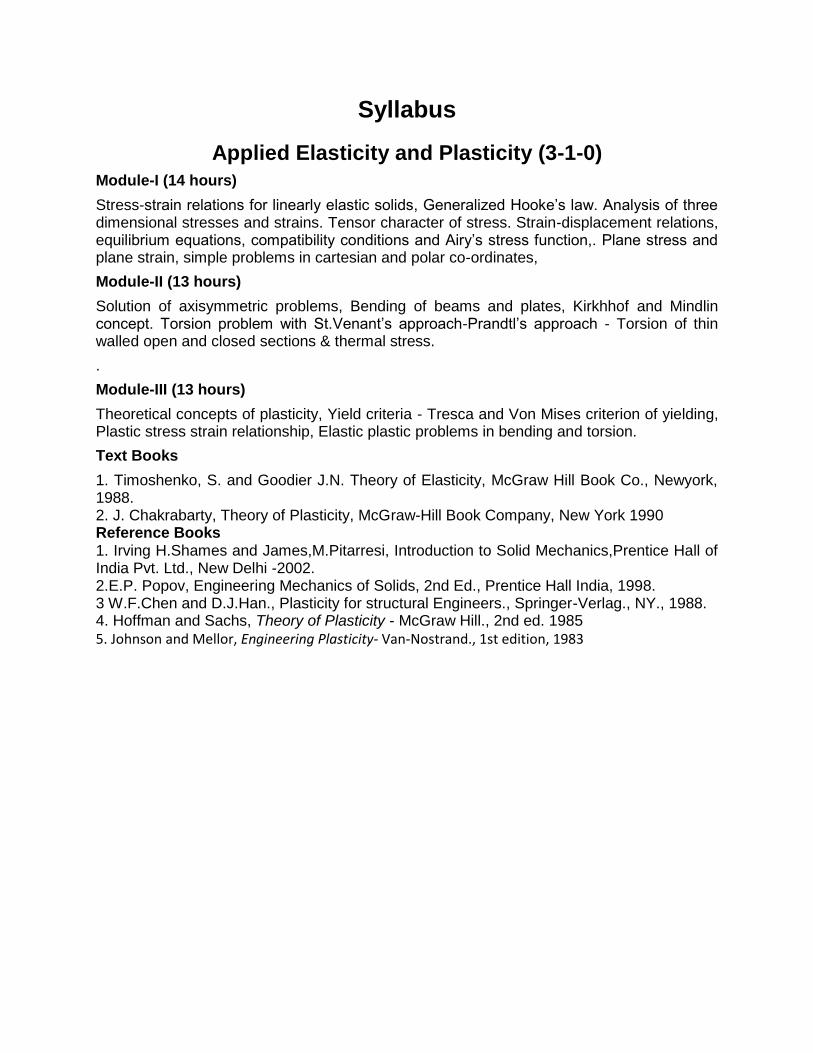
Syllabus
Applied Elasticity and Plasticity (3-1-0)
Module-I (14 hours)
Stress-strain relations for linearly elastic solids, Generalized Hooke’s law. Analysis of three dimensional stresses and strains. Tensor character of stress. Strain-displacement relations, equilibrium equations, compatibility conditions and Airy’s stress function,. Plane stress and plane strain, simple problems in cartesian and polar co-ordinates,
Module-II (13 hours)
Solution of axisymmetric problems, Bending of beams and plates, Kirkhhof and Mindlin concept. Torsion problem with St.Venant’s approach-Prandtl’s approach - Torsion of thin walled open and closed sections & thermal stress.
.
Module-III (13 hours)
Theoretical concepts of plasticity, Yield criteria - Tresca and Von Mises criterion of yielding, Plastic stress strain relationship, Elastic plastic problems in bending and torsion.
Text Books
1. Timoshenko, S. and Goodier J.N. Theory of Elasticity, McGraw Hill Book Co., Newyork, 1988. 2. J. Chakrabarty, Theory of Plasticity, McGraw-Hill Book Company, New York 1990 Reference Books 1. Irving H.Shames and James,M.Pitarresi, Introduction to Solid Mechanics,Prentice Hall of India Pvt. Ltd., New Delhi -2002. 2.E.P. Popov, Engineering Mechanics of Solids, 2nd Ed., Prentice Hall India, 1998. 3 W.F.Chen and D.J.Han., Plasticity for structural Engineers., Springer-Verlag., NY., 1988. 4. Hoffman and Sachs, Theory of Plasticity - McGraw Hill., 2nd ed. 1985
5. Johnson and Mellor, Engineering Plasticity- Van-Nostrand., 1st edition, 1983

Module-I Elasticity: All structural materials possess to a certain extent the property of elasticity i.e. if external forces, producing deformation of a structure, don’t exceed a certain limit; the deformation disappears with the removal of the forces. In this course it will be assumed that the bodies undergoing the action of external forces are perfectly elastic, i.e. that they resume their initial form completely after removal of forces.
The simplest mechanical test consists of placing a standardized specimen
with its ends in the grips of a tensile testing machine and then applying load
under controlled conditions. Uniaxial loading conditions are thus
approximately obtained. A force balance on a small element of the
specimen yields the longitudinal (true) stress as
𝜎 =𝐹
𝐴
Where, F is the applied force and A is the (instantaneous) cross sectional
area of the specimen. Alternatively, if the initial cross sectional area A0 is
used, one obtains the engineering stress
𝜎𝑒 =𝐹
𝐴0
For loading in the elastic regime, for most engineering materials 𝜎𝑒 = 𝜎
Stress: A body under the action of external forces, undergoes distortion
and the effect due to this system of forces is transmitted throughout the
body developing internal forces in it. To examine these internal forces at a
point O in Figure (a), inside the body, consider a plane MN passing through
the point O. If the plane is divided into a number of small areas, as in the
Figure (b), and the forces acting on each of these are measured, it will be
observed that these forces vary from one small area to the next. On the
small area DA at point O, a force DF will be acting as shown in the Figure
2.1 (b). From this the concept of stress as the internal force per unit area
can be understood. Assuming that the material is continuous, the term
"stress" at any point across a small area ∆A can be defined by the limiting
equation as below.
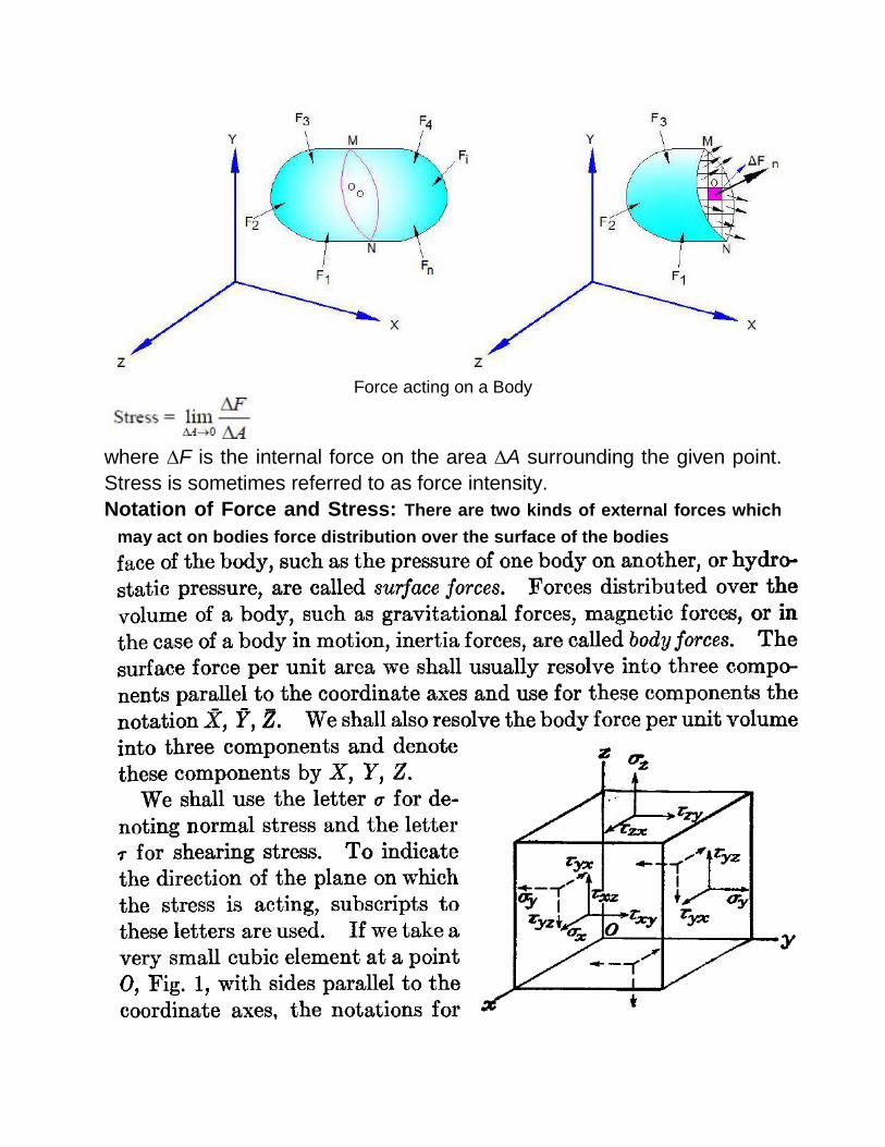
Force acting on a Body
where ∆F is the internal force on the area ∆A surrounding the given point.
Stress is sometimes referred to as force intensity.
Notation of Force and Stress: There are two kinds of external forces which
may act on bodies force distribution over the surface of the bodies
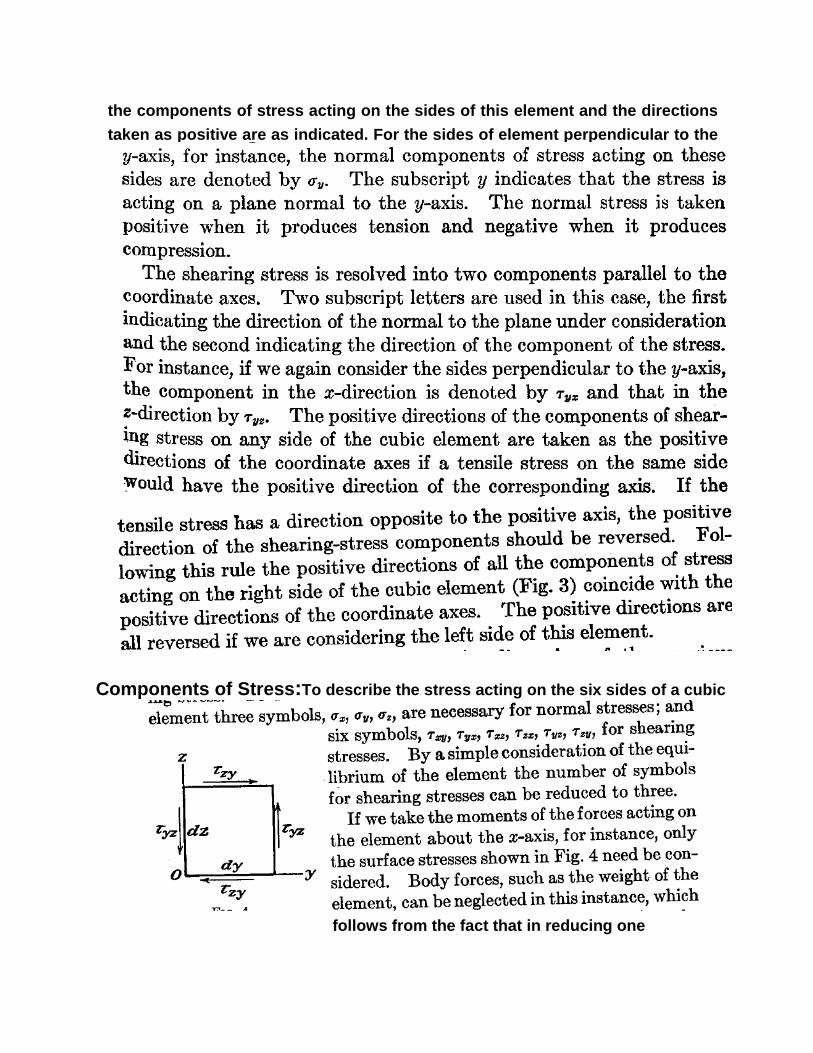
the components of stress acting on the sides of this element and the directions
taken as positive are as indicated. For the sides of element perpendicular to the
Components of Stress:To describe the stress acting on the six sides of a cubic
follows from the fact that in reducing one

Hence for two perpendicular sides of a cubic elements the components of
Components of strain:
elastic body. If the body undergoes a deformation and 𝒖, 𝒗, 𝒘
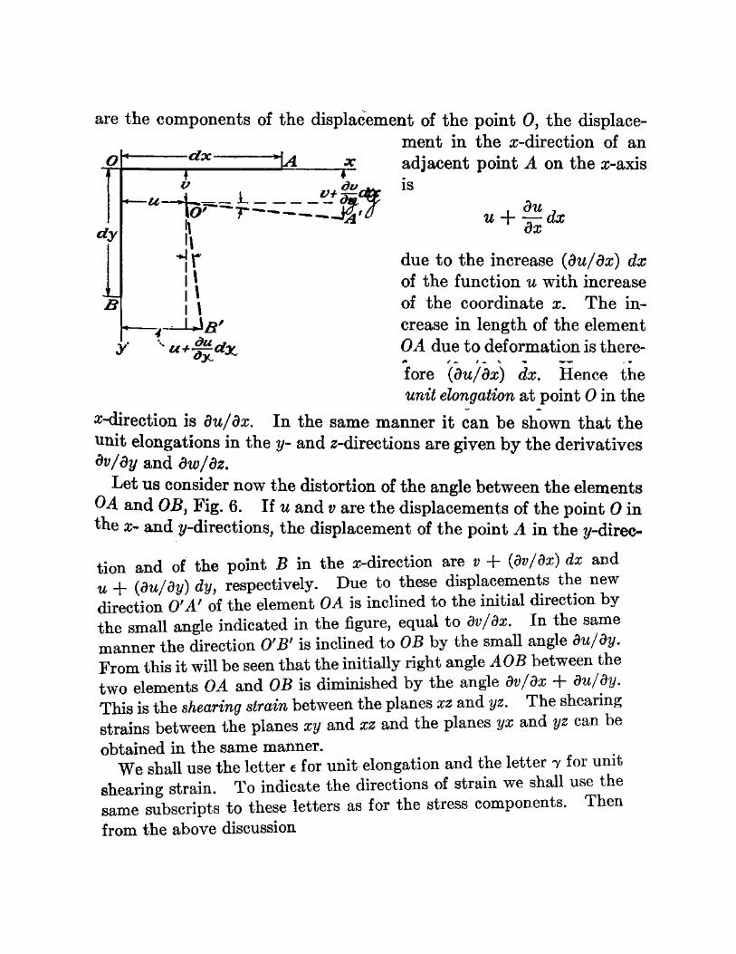

the angle between any two can be calculated later on.
The six quantities 𝜖𝑥, 𝜖𝑦, 𝜖𝑧 , 𝛾𝑥𝑦, 𝛾𝑥𝑧 𝑎𝑛𝑑 𝛾𝑦𝑧 are called the components of strain.
Generalized Hooke’s Law:
Linear elastic behavior in the tension test is well described by Hooke's law, namely
𝜎 = 𝐸𝜀 where E is the modulus of elasticity or Young's modulus. For most materials, this is a large number of the order of 1011 Pa. The statement that the component of stress at a given point inside a linear elastic medium are linear homogeneous functions of the strain components at the point is known as the generalized Hooke's law. Mathematically, this implies that

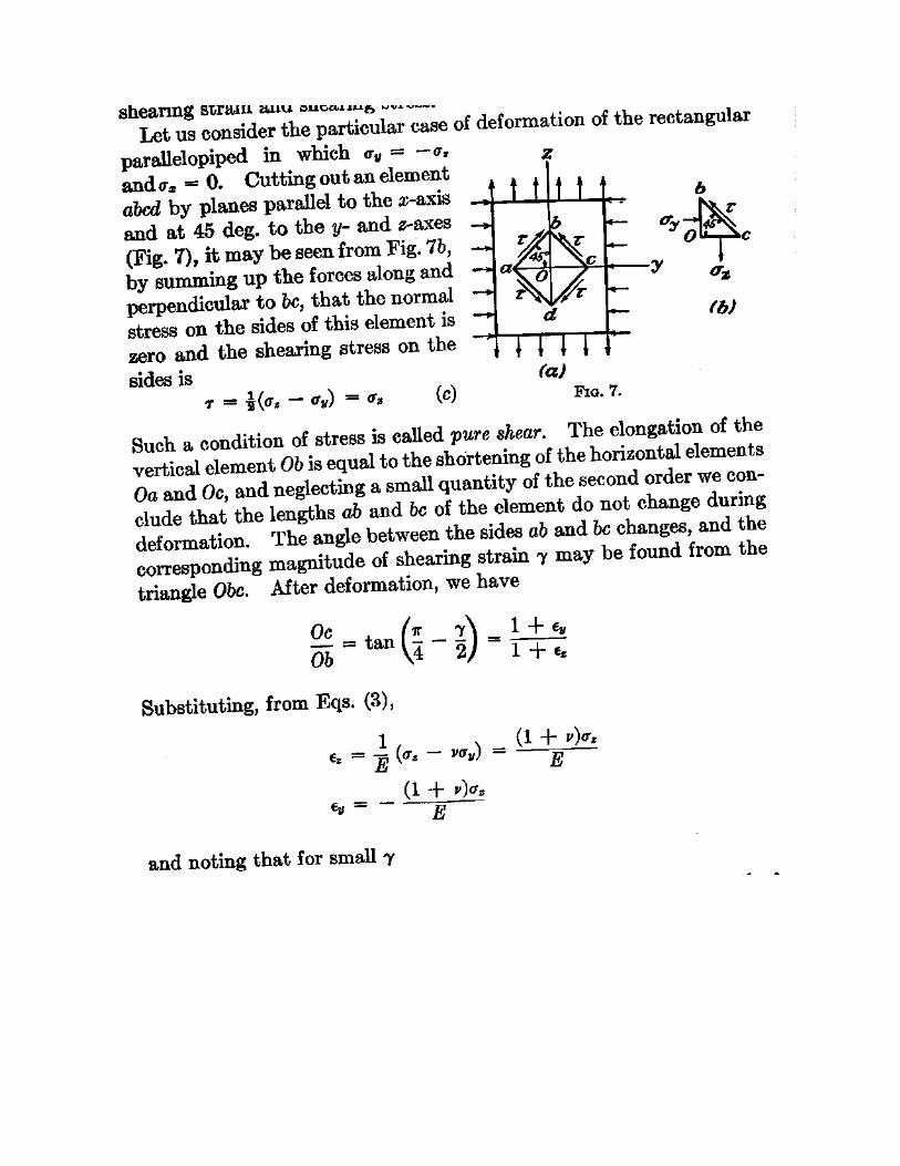
Stress-Strain relations for Isotropic-elastic solid:
this formula reduced to its simplest form as
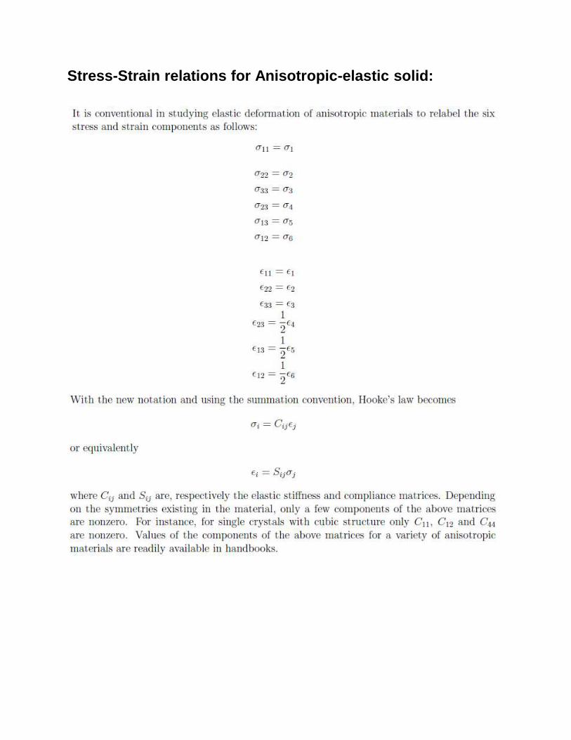
Stress-Strain relations for Anisotropic-elastic solid:
Stress tensor:
Let O be the point in a body shown in Figure 2.1 (a). Passing through that point, infinitely many planes may be drawn. As the resultant forces acting on these planes is the same, the stresses on these planes are different because the areas and the inclinations of these planes are different. Therefore, for a complete description of stress, we have to specify not only its magnitude, direction and sense but also the surface on which it acts. For this reason, the stress is called a "Tensor".
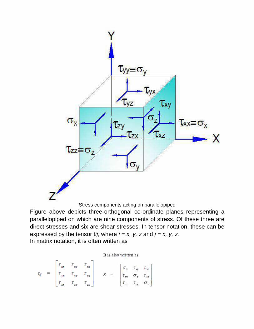
Stress components acting on parallelopiped
Figure above depicts three-orthogonal co-ordinate planes representing a
parallelopiped on which are nine components of stress. Of these three are
direct stresses and six are shear stresses. In tensor notation, these can be
expressed by the tensor tij, where i = x, y, z and j = x, y, z.
In matrix notation, it is often written as
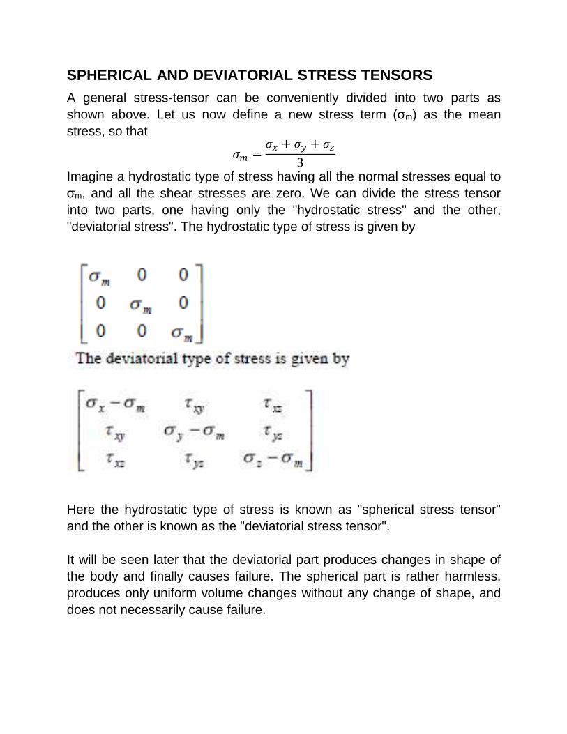
SPHERICAL AND DEVIATORIAL STRESS TENSORS
A general stress-tensor can be conveniently divided into two parts as
shown above. Let us now define a new stress term (σm) as the mean
stress, so that
𝜎𝑚 =𝜎𝑥 + 𝜎𝑦 + 𝜎𝑧
3
Imagine a hydrostatic type of stress having all the normal stresses equal to
σm, and all the shear stresses are zero. We can divide the stress tensor
into two parts, one having only the "hydrostatic stress" and the other,
"deviatorial stress". The hydrostatic type of stress is given by
Here the hydrostatic type of stress is known as "spherical stress tensor"
and the other is known as the "deviatorial stress tensor".
It will be seen later that the deviatorial part produces changes in shape of
the body and finally causes failure. The spherical part is rather harmless,
produces only uniform volume changes without any change of shape, and
does not necessarily cause failure.

TYPES OF STRESS
Stresses may be classified in two ways, i.e., according to the type of body
on which they act, or the nature of the stress itself. Thus stresses could be
one-dimensional, two-dimensional or three-dimensional as shown in the
Figure (a), (b) and (c).
(a) One-dimensional Stress
(b) Two-dimensional Stress (c) Three-dimensional Stress
Types of Stress
TWO-DIMENSIONAL STRESS AT A POINT
A two-dimensional state-of-stress exists when the stresses and body forces are
independent of one of the co-ordinates. Such a state is described by stresses σx , σy
and τxy and the X and Y body forces (Here z is taken as the independent co-
ordinate axis).
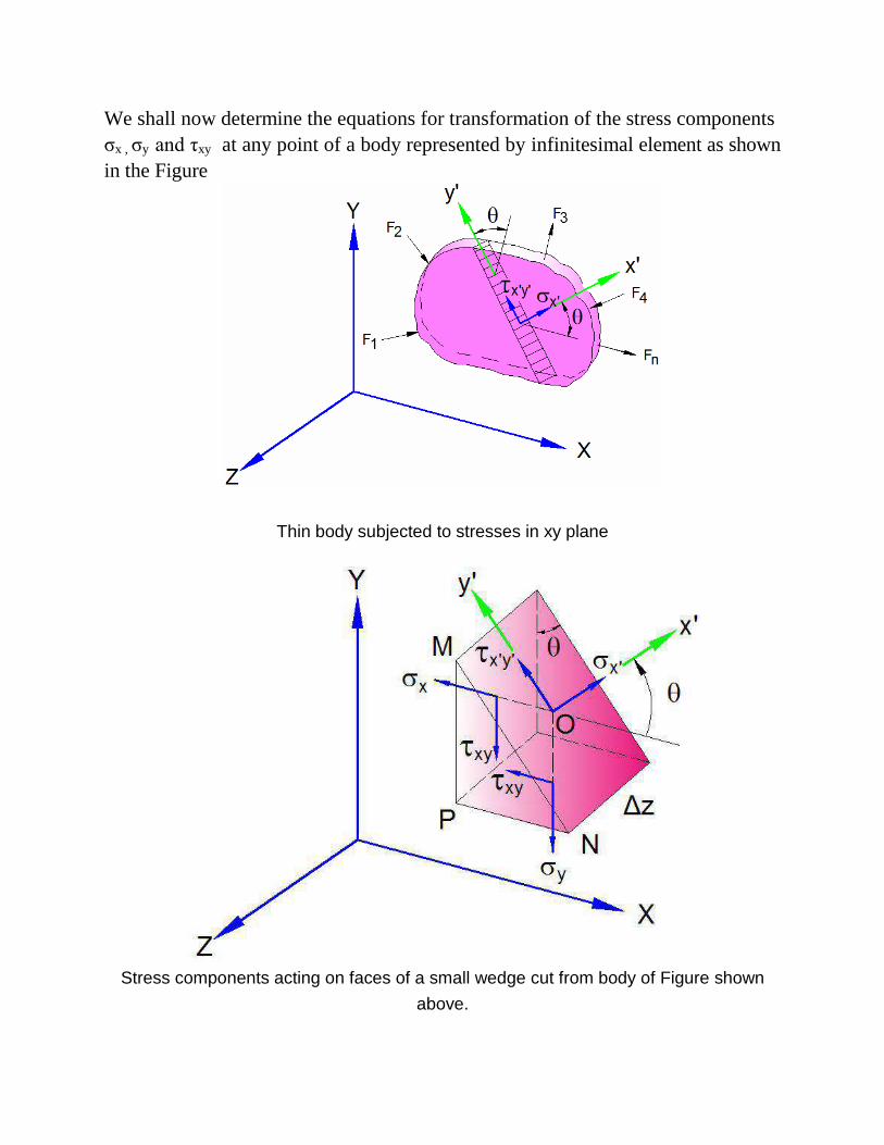
We shall now determine the equations for transformation of the stress components
σx , σy and τxy at any point of a body represented by infinitesimal element as shown
in the Figure
Thin body subjected to stresses in xy plane
Stress components acting on faces of a small wedge cut from body of Figure shown
above.
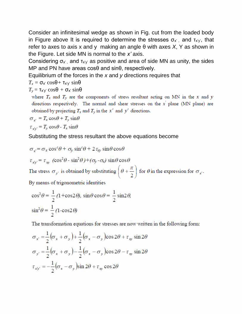
Consider an infinitesimal wedge as shown in Fig. cut from the loaded body
in Figure above It is required to determine the stresses σx’ , and τx’y’, that
refer to axes to axis x and y making an angle θ with axes X, Y as shown in
the Figure. Let side MN is normal to the x’ axis.
Considering σx’ , and τx’y’ as positive and area of side MN as unity, the sides
MP and PN have areas cosθ and sinθ, respectively.
Equilibrium of the forces in the x and y directions requires that
Tx = σx’ cosθ+ τx’y’ sinθ
Ty = τx’y’ cosθ + σx’ sinθ
Substituting the stress resultant the above equations become

Principal stress in two dimensions:
is applied to equation of yielding
These are the principal directions along which the principal or maximum
and minimum normal stress act.
A principal plane is thus a plane on which the shear stress is zero. The
principal stresses are determined by the equation
Analysis of three dimensional stresses and strains
Consider a cube of infinitesimal dimensions shown in figure; all stresses acting on
this cube are identified on the diagram. The subscripts (τ) are the shear stress,
associate the stress with a plane perpendicular to a given axis, the second designate
the direction of the stress, i.e.

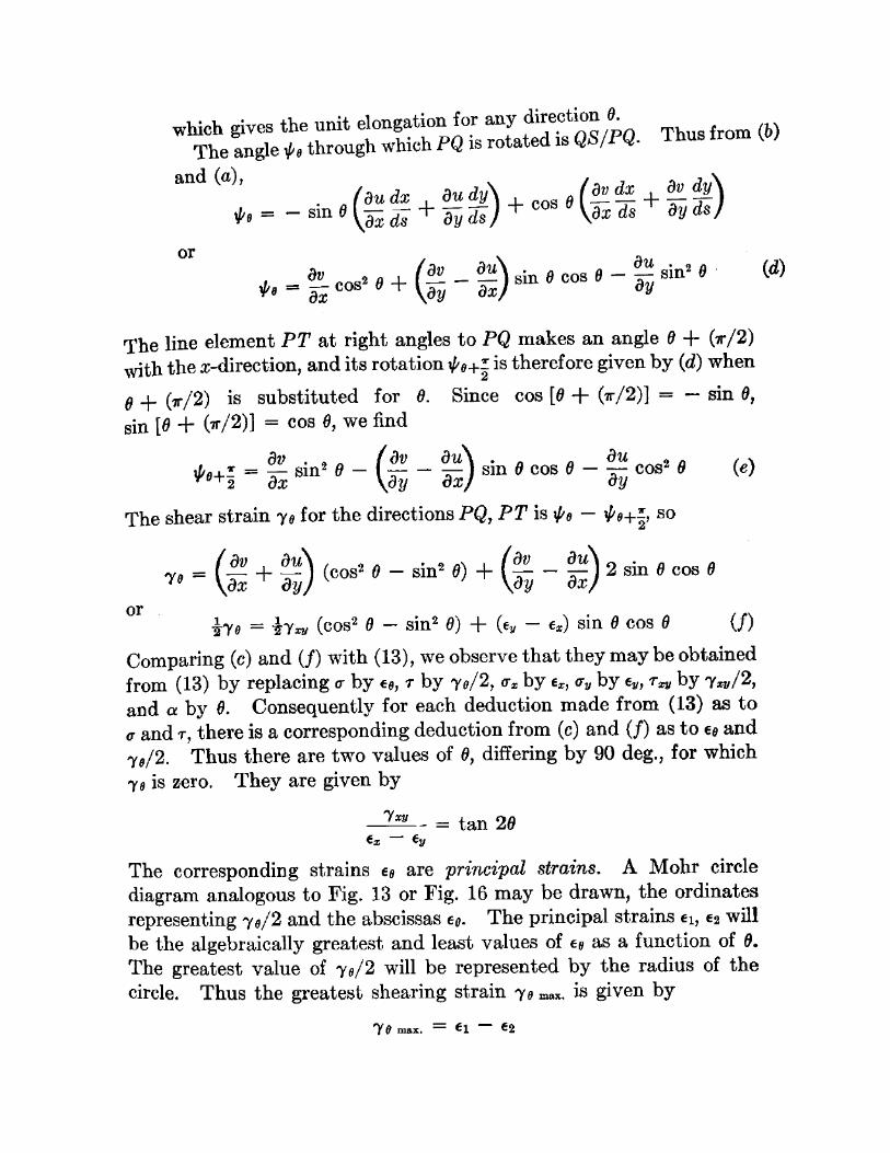
Strain-displacement relations: When the strain components 𝜖𝑥, 𝜖𝑦 and 𝛾𝑥𝑦 at a point are known, the unit
elongation or displacement for any direction and the decrease of a right
angle (the shearing strain) of the any orientationat the point can be found.
A line PQ as shown in figure below between the points (x,y) , (x+dx, y+dy)
is translated, stretched (contracted) and rotated into the line element P’Q’

when the deformation occurs. The displacement component of P are u,v
those of Q are

Equilibrium equations
Consider the equilibrium of a small
rectangular block of edges h,k and
unity as shown in the figure.
The stresses acting on the faces
1,2,3,4 and their positive directions
are indicated in the figure. On
account of the deviation of stress

Boundary Conditions: Equations (18) or (19) must be satisfied
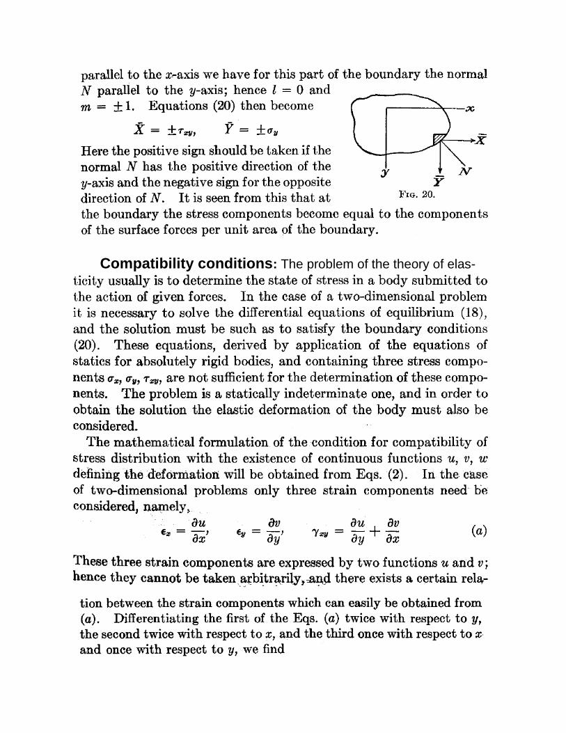
Compatibility conditions: The problem of the theory of elas-
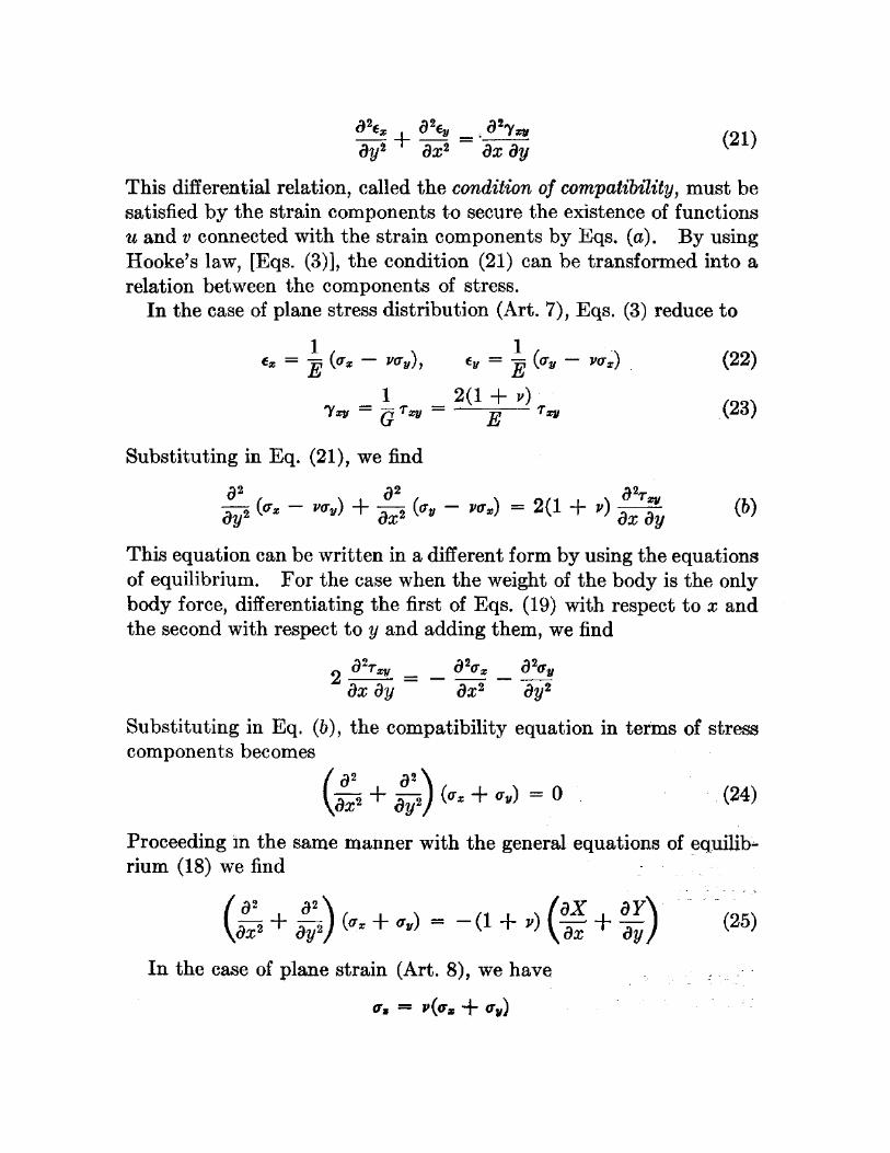
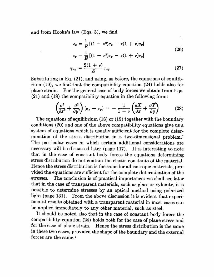
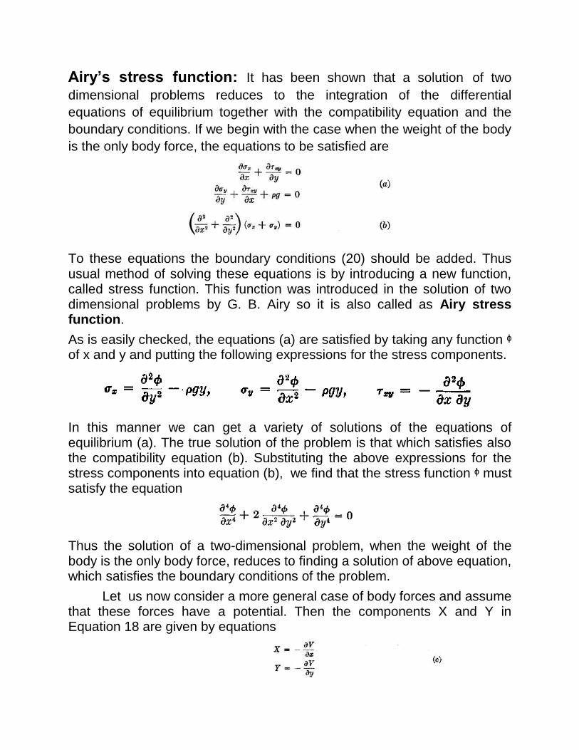
Airy’s stress function: It has been shown that a solution of two
dimensional problems reduces to the integration of the differential
equations of equilibrium together with the compatibility equation and the
boundary conditions. If we begin with the case when the weight of the body
is the only body force, the equations to be satisfied are
To these equations the boundary conditions (20) should be added. Thus usual method of solving these equations is by introducing a new function, called stress function. This function was introduced in the solution of two dimensional problems by G. B. Airy so it is also called as Airy stress function.
As is easily checked, the equations (a) are satisfied by taking any function ᶲ of x and y and putting the following expressions for the stress components.
In this manner we can get a variety of solutions of the equations of equilibrium (a). The true solution of the problem is that which satisfies also the compatibility equation (b). Substituting the above expressions for the stress components into equation (b), we find that the stress function ᶲ must satisfy the equation
Thus the solution of a two-dimensional problem, when the weight of the body is the only body force, reduces to finding a solution of above equation, which satisfies the boundary conditions of the problem.
Let us now consider a more general case of body forces and assume that these forces have a potential. Then the components X and Y in Equation 18 are given by equations
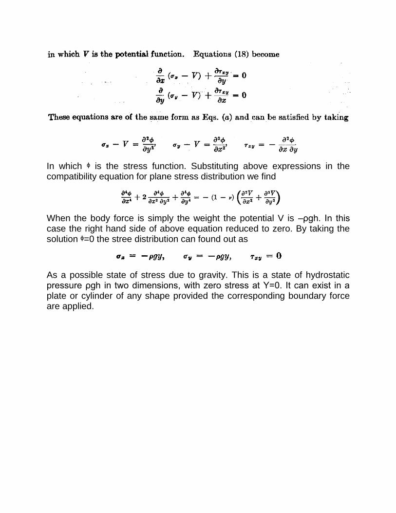
In which ᶲ is the stress function. Substituting above expressions in the compatibility equation for plane stress distribution we find
When the body force is simply the weight the potential V is –ρgh. In this case the right hand side of above equation reduced to zero. By taking the solution ᶲ=0 the stree distribution can found out as
As a possible state of stress due to gravity. This is a state of hydrostatic pressure ρgh in two dimensions, with zero stress at Y=0. It can exist in a plate or cylinder of any shape provided the corresponding boundary force are applied.
Module-II
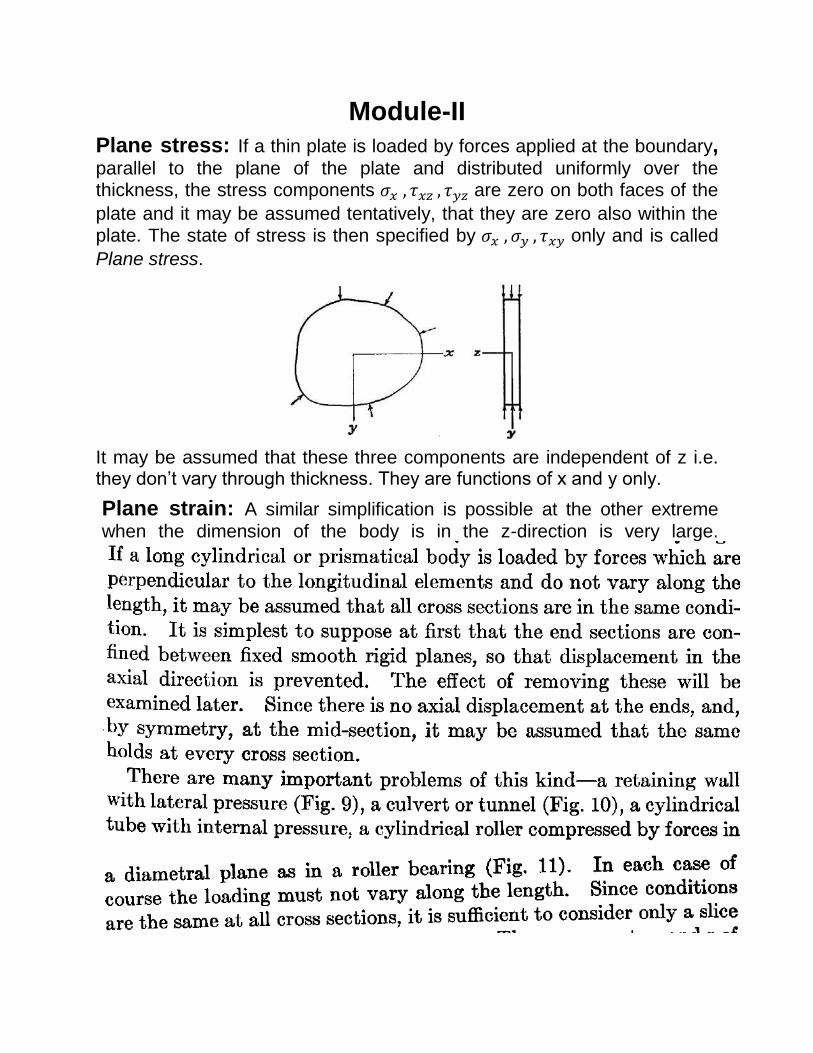
Plane stress: If a thin plate is loaded by forces applied at the boundary, parallel to the plane of the plate and distributed uniformly over the thickness, the stress components 𝜎𝑥 , 𝜏𝑥𝑧 , 𝜏𝑦𝑧 are zero on both faces of the
plate and it may be assumed tentatively, that they are zero also within the plate. The state of stress is then specified by 𝜎𝑥 , 𝜎𝑦 , 𝜏𝑥𝑦 only and is called
Plane stress.
It may be assumed that these three components are independent of z i.e. they don’t vary through thickness. They are functions of x and y only.
Plane strain: A similar simplification is possible at the other extreme
when the dimension of the body is in the z-direction is very large.
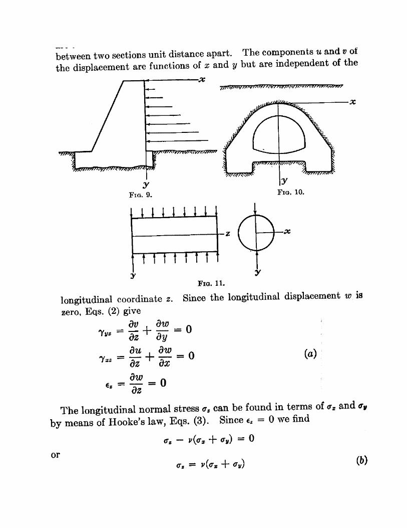

Simple problems in cartesian and polar co-ordinates
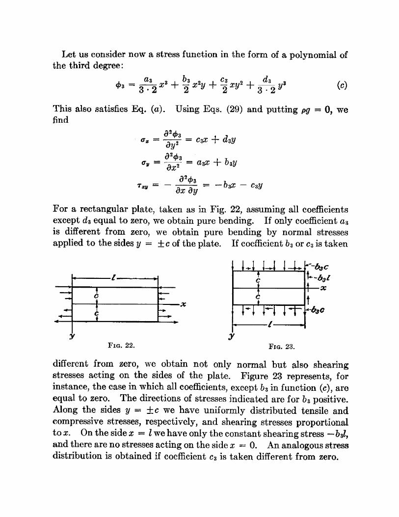
Solution by polynomials: it has been shown that the solution


ST. VENANT’S PRINCIPLE
For the purpose of analysing the statics or dynamics of a body, one force
system may be replaced by an equivalent force system whose force and
moment resultants are identical. Such force resultants, while equivalent
need not cause an identical distribution of strain, owing to difference in the
arrangement of forces. St. Venant’s principle permits the use of an
equivalent loading for the calculation of stress and strain.
St. Venant’s principle states that if a certain system of forces acting on a
portion of the surface of a body is replaced by a different system of forces
acting on the same portion of the body, then the effects of the two different
systems at locations sufficiently far distant from the region of application of
forces, are essentially the same, provided that the two systems of forces
are statically equivalent (i.e., the same resultant force and the same
resultant moment). St. Venant principle is very convenient and useful in
obtaining solutions to many engineering problems in elasticity. The
principle helps to the great extent in prescribing the boundary conditions
very precisely when it is very difficult to do so.
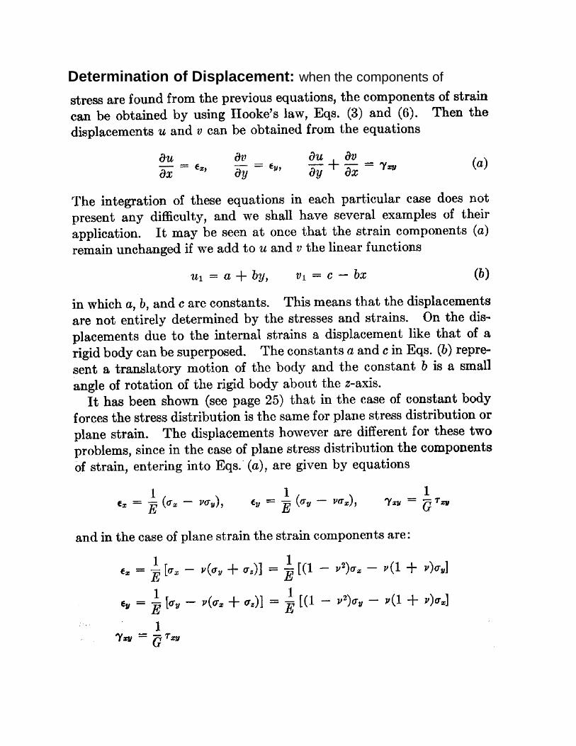
Determination of Displacement: when the components of

unchanged.
Two Dimensional Problems in Polar Coordinate System In any elasticity problem the proper choice of the co-ordinate system is
extremely important since this choice establishes the complexity of the
mathematical expressions employed to satisfy the field equations and the
boundary conditions. In order to solve two dimensional elasticity problems
by employing a polar co-ordinate reference frame, the equations of
equilibrium, the definition of Airy’s Stress function, and one of the stress
equations of compatibility must be established in terms of Polar Co-
ordinates. STRAIN-DISPLACEMENT RELATIONS Case 1: For Two Dimensional State of Stress
Deformed element in two dimensions
Consider the deformation of the infinitesimal element ABCD, denoting r and q displacements by u and v respectively. The general deformation experienced by an element may be regarded as composed of (1) a change in the length of the sides, and (2) rotation of the sides as shown in the figure above.

Referring to the figure, it is observed that a displacement "u" of side AB results in both radial and tangential strain.

Case 2: For three dimensional stress state

Compatibility Equation:
We have from strain displacement relation
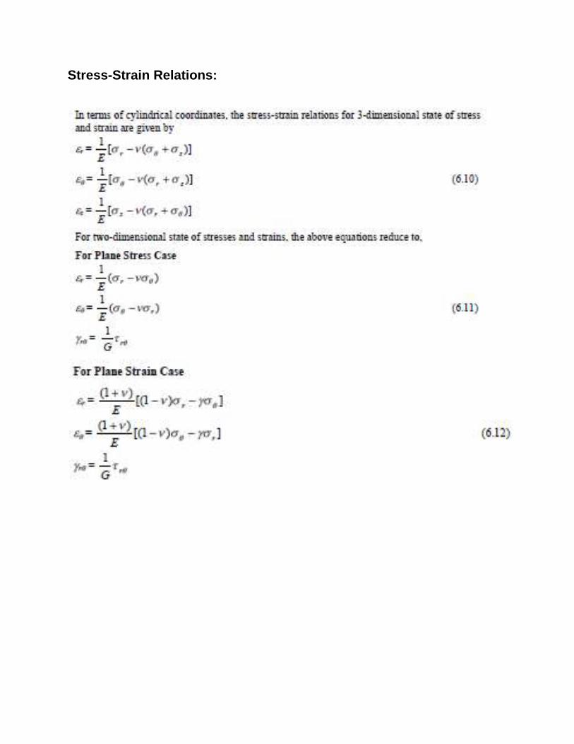
Stress-Strain Relations:

Airy’s Stress function:

AXISYMMETRIC PROBLEMS
Many engineering problems involve solids of revolution subjected to axially
symmetric loading. The examples are a circular cylinder loaded by uniform
internal or external pressure or other axially symmetric loading, and a semi-
infinite half space loaded by a circular area, for example a circular footing
on a soil mass. It is convenient to express these problems in terms of the
cylindrical co-ordinates. Because of symmetry, the stress components are
independent of the angular (q) co-ordinate; hence, all derivatives with
respect to q vanish and the components 𝑣, 𝛾𝑟𝜃 , 𝛾𝜃𝑧, 𝜏𝑟𝜃 𝑎𝑛𝑑 𝜏𝜃𝑧 are zero.
The non-zero stress components are𝜎𝑟 , 𝜎𝜃 , , 𝜎𝑧 𝑎𝑛𝑑 𝜏𝑟𝑧.

Axisymmetric problems
Thick walled cylinder subjected to internal and external pressure:
Consider a cylinder of inner radius ‘a’ and outer radius ‘b’ as shown in figure below.
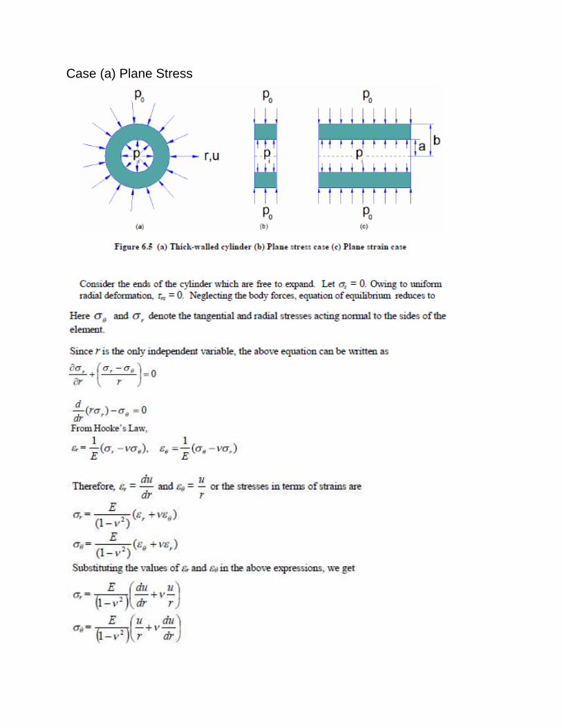
Case (a) Plane Stress
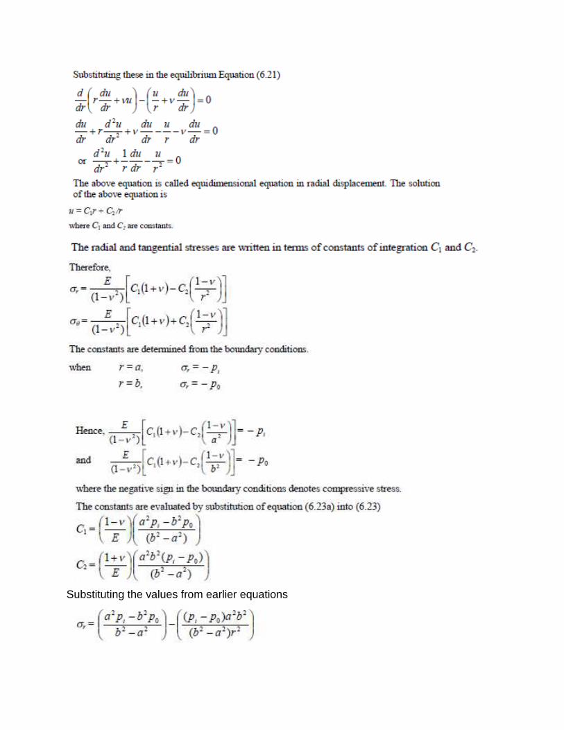
Substituting the values from earlier equations
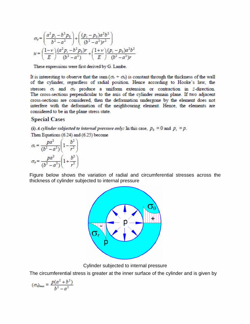
Figure below shows the variation of radial and circumferential stresses across the thickness of cylinder subjected to internal pressure
Cylinder subjected to internal pressure
The circumferential stress is greater at the inner surface of the cylinder and is given by
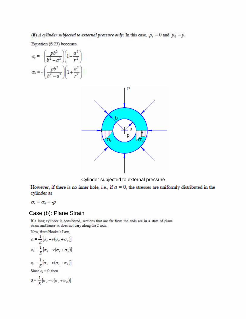
Cylinder subjected to external pressure
Case (b): Plane Strain


It is observed that the values of 𝜎𝑟 𝑎𝑛𝑑 𝜎𝜃 are identical to those in plane stress case. But in plane stress case, 𝜎𝑧 =0, where as in plane strain case 𝜎𝑧 has a constant value given by above equation.
Rotating Discs of Uniform thickness:
The equation of equilibrium given by 𝜕𝜎𝑟
𝜕𝑟+ (
𝜎𝑟−𝜎𝜃
𝑟) + 𝐹𝑟 = 0 (a)
is used to treat the case of a rotating disk, provided that the centrifugal "inertia force" is included as a body force. It is assumed that the stresses

induced by rotation are distributed symmetrically about the axis of rotation and also independent of disk thickness.Thus, application of equation (a), with the body force per unit volume Fr equated to the centrifugal force
𝜌𝜔2𝑟, yields 𝜕𝜎𝑟
𝜕𝑟+ (
𝜎𝑟 − 𝜎𝜃
𝑟) + 𝜌𝜔2𝑟 = 0
Where 𝜌 is the mass density and 𝜔 is the constant angular speed of the disk in rad/sec. the above equation can be written as
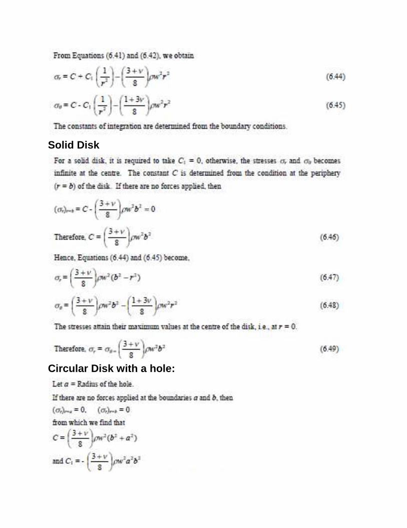
Solid Disk
Circular Disk with a hole:
Stress concentration
While discussing the case of simple tension and compression, it has been
assumed that the bar has a prismatical form. Then for centrally applied
forces, the stress at some distance from the ends is uniformly distributed
over the cross-section. Abrupt changes in cross-section give rise to great
irregularities in stress distribution. These irregularities are of particular
importance in the design of machine parts subjected to variable external
forces and to reversal of stresses. If there exists in the structural or
machine element a discontinuity that interrupts the stress path, the stress
at that discontinuity may be considerably greater than the nominal stress
on the section; thus there is a “Stress Concentration” at the discontinuity.
The ratio of the maximum stress to the nominal stress on the section is
known as the 'Stress Concentration Factor'. Thus, the expression for the
maximum normal stress in a centrically loaded member becomes
where A is either gross or net area (area at the reduced section), K = stress
concentration factor and P is the applied load on the member. In Figures
6.8 (a), 6.8(b) and 6.8(c), the type of discontinuity is shown and in Figures

6.8(d), 6.8(e) and 6.8(f) the approximate distribution of normal stress on a
transverse plane is shown.
Stress concentration is a matter, which is frequently overlooked by
designers. The high stress concentration found at the edge of a hole is of
great practical importance. As an example, holes in ships decks may be
mentioned. When the hull of a ship is bent, tension or compression is
produced in the decks and there is a high stress concentration at the holes.
Under the cycles of stress produced by waves, fatigue of the metal at the
overstressed portions may result finally in fatigue cracks.
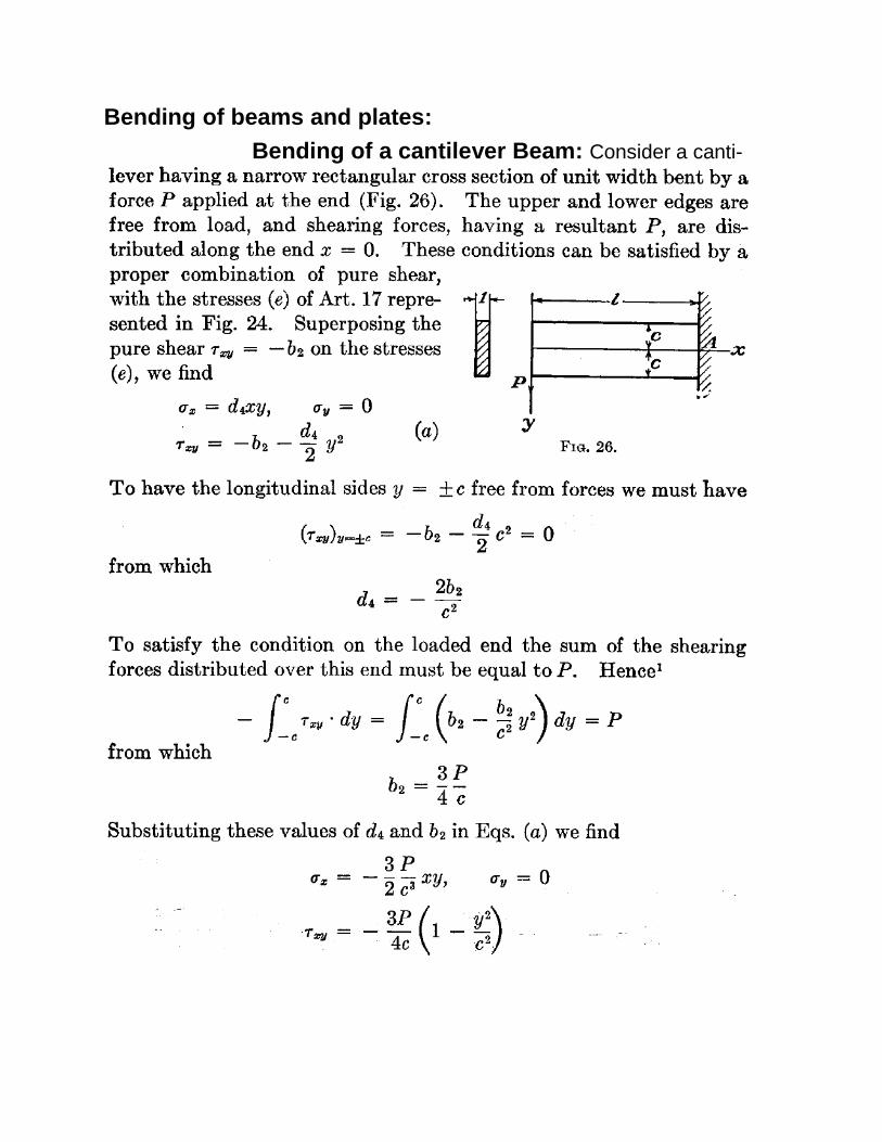
Bending of beams and plates:
Bending of a cantilever Beam: Consider a canti-


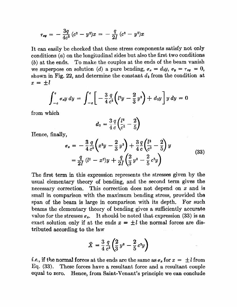
Bending of beam by uniform loading: Let a beam of narrow


Kirkhhof and Mindlin concept

Module-III.
Torsion of Prismatic Bars (St.Venant’s approach)
From the study of elementary strength of materials, two important
expressions related to the torsion of circular bars were developed. They are
The following are the assumptions associated with the elementary
approach in deriving above equations.
1. The material is homogeneous and obeys Hooke’s Law.
2. All plane sections perpendicular to the longitudinal axis remain plane
following the application of a torque, i.e., points in a given cross-sectional
plane remain in that plane after twisting.
3. Subsequent to twisting, cross-sections are undistorted in their individual
planes, i.e., the shearing strain varies linearly with the distance from the
central axis.
4. Angle of twist per unit length is constant.
In most cases, the members that transmit torque, such as propeller shaft
and torque tubes of power equipment, are circular or turbular in cross-
section.
But in some cases, slender members with other than circular cross-
sections are used. These are shown in the Figure 7.0.
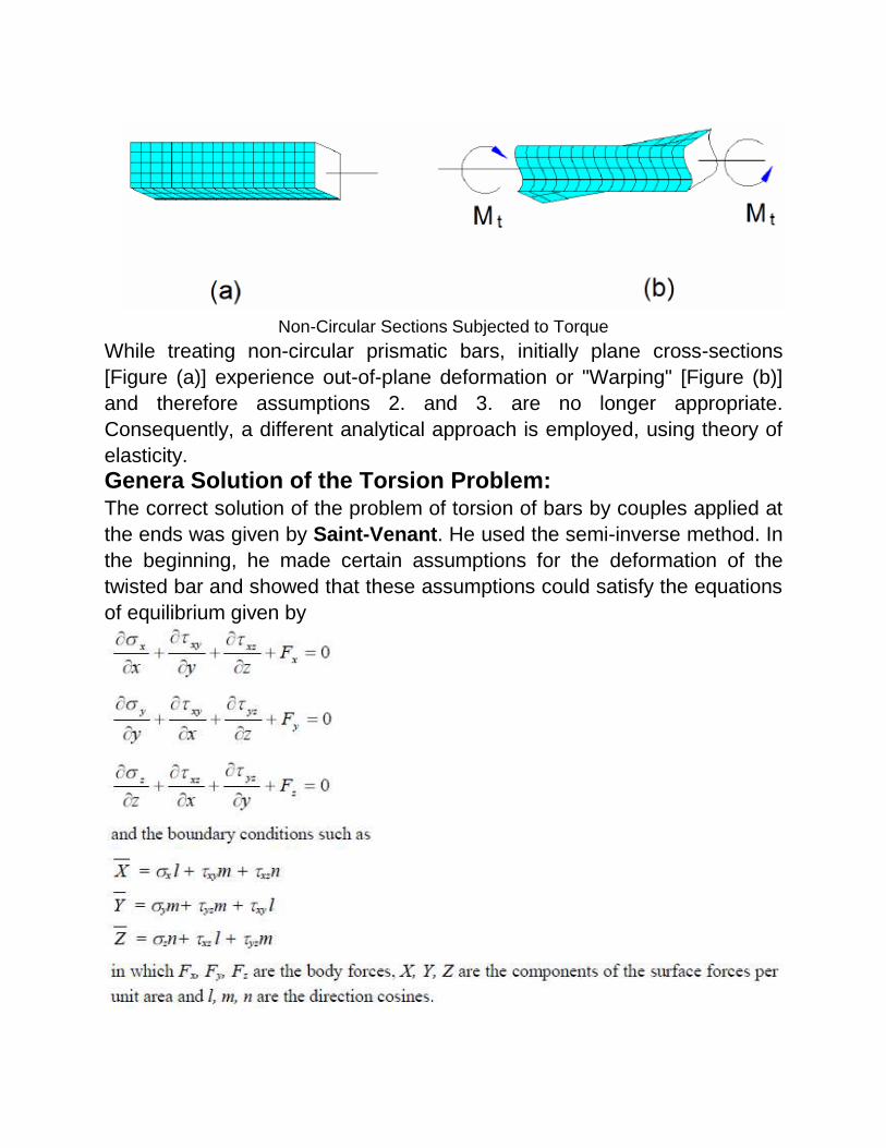
Non-Circular Sections Subjected to Torque
While treating non-circular prismatic bars, initially plane cross-sections
[Figure (a)] experience out-of-plane deformation or "Warping" [Figure (b)]
and therefore assumptions 2. and 3. are no longer appropriate.
Consequently, a different analytical approach is employed, using theory of
elasticity.
Genera Solution of the Torsion Problem: The correct solution of the problem of torsion of bars by couples applied at
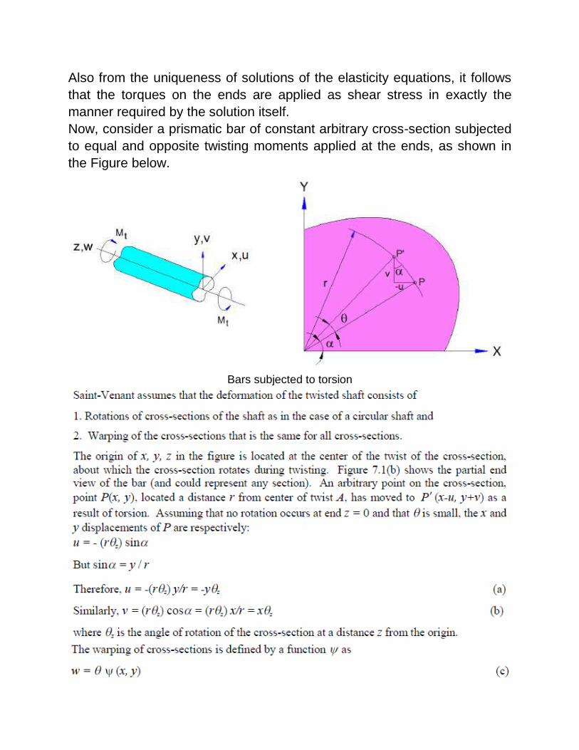
the ends was given by Saint-Venant. He used the semi-inverse method. In
the beginning, he made certain assumptions for the deformation of the
twisted bar and showed that these assumptions could satisfy the equations
of equilibrium given by
Also from the uniqueness of solutions of the elasticity equations, it follows
that the torques on the ends are applied as shear stress in exactly the
manner required by the solution itself.
Now, consider a prismatic bar of constant arbitrary cross-section subjected
to equal and opposite twisting moments applied at the ends, as shown in
the Figure below.
Bars subjected to torsion


Therefore the stress in a bar of arbitrary section may be determined by solving above
Equations along with the given boundary conditions.
Boundary Conditions:
which means that the resultant shearing stress at the boundary is directed along the
tangent to the boundary, as shown in the Figure below.
Cross-section of the bar & Boundary conditions

The above equation becomes
Thus each problem of torsion is reduced to the problem of finding a function y satisfying
equation and the boundary condition given above.
Stress function method: (Prandtl approach)
As in the case of beams, the torsion problem formulated above is commonly solved by
introducing a single stress function. This procedure has the advantage of leading to
simpler boundary conditions as compared to Equation given above. The method is
proposed by Prandtl. In this method, the principal unknowns are the stress components
rather than the displacement components as in the previous approach.
With this stress function, (called Prandtl torsion stress function), the third
condition is also satisfied. The assumed stress components, if they are to
be proper elasticity solutions, have to satisfy the compatibility conditions.
We can substitute these directly into the stress equations of compatibility.
Alternately, we can determine the strains corresponding to the assumed
stresses and then apply the strain compatibility conditions.
Therefore from above Equations , we have
The boundary condition becomes, introducing above Equation.
This shows that the stress function f must be constant along the boundary of the cross
section. In the case of singly connected sections, example, for solid bars, this constant
can be arbitrarily chosen. Since the stress components depend only on the differentials
of ᶲ, for a simply connected region, no loss of generality is involved in assuming ᶲ = 0 on
S. However, for a multi-connected region, example shaft having holes, certain additional
conditions of compatibility are imposed. Thus the determination of stress distribution
over a cross-section of a twisted bar is used in finding the function f that satisfies above
Equation and is zero at the boundary.
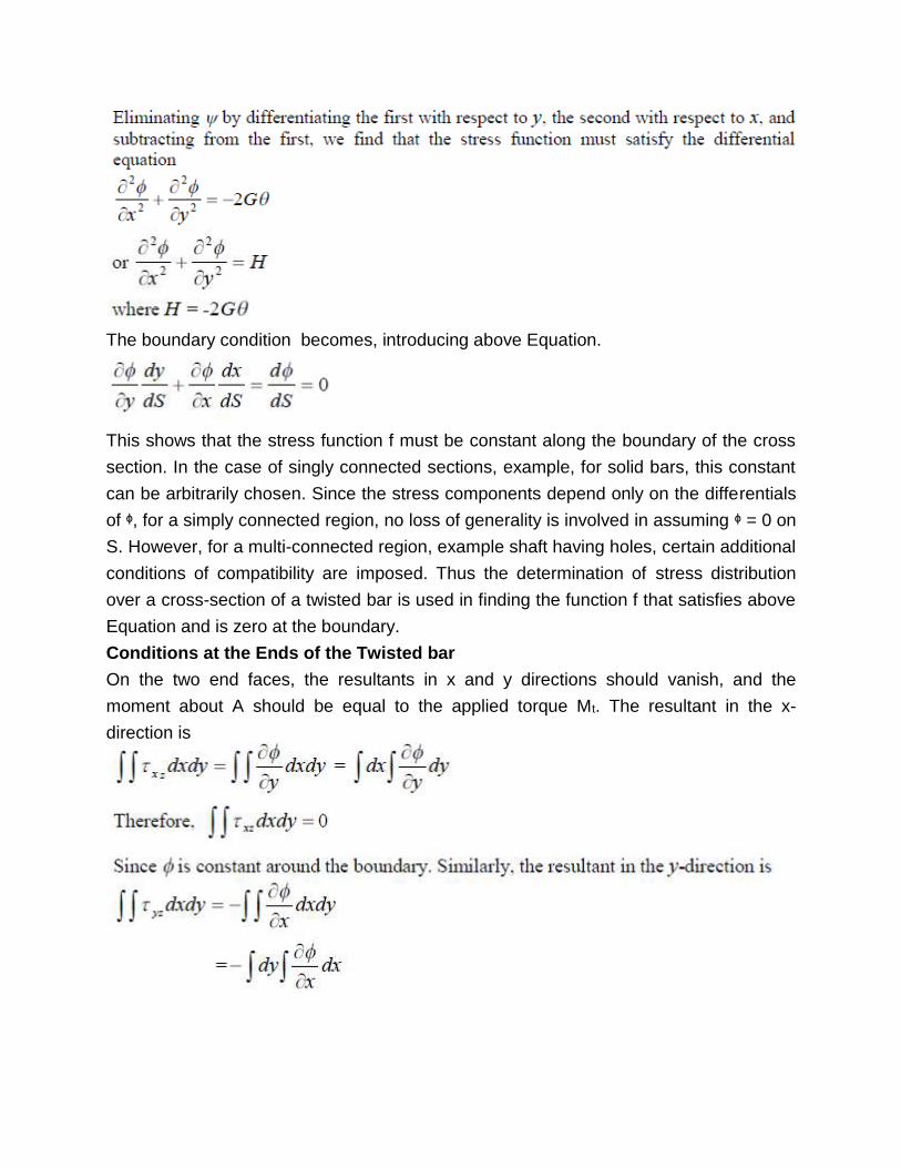
Conditions at the Ends of the Twisted bar
On the two end faces, the resultants in x and y directions should vanish, and the
moment about A should be equal to the applied torque Mt. The resultant in the x-
direction is
Thus the resultant of the forces distributed over the ends of the bar is zero, and these
forces represent a couple the magnitude of which is
Hence, we observe that each of the integrals in Equation contributing one half of the
torque due to txz and the other half due to tyz. Thus all the differential equations and
boundary conditions are satisfied if the stress function ᶲ obeys above Equations and the
solution obtained in this manner is the exact solution of the torsion problem.
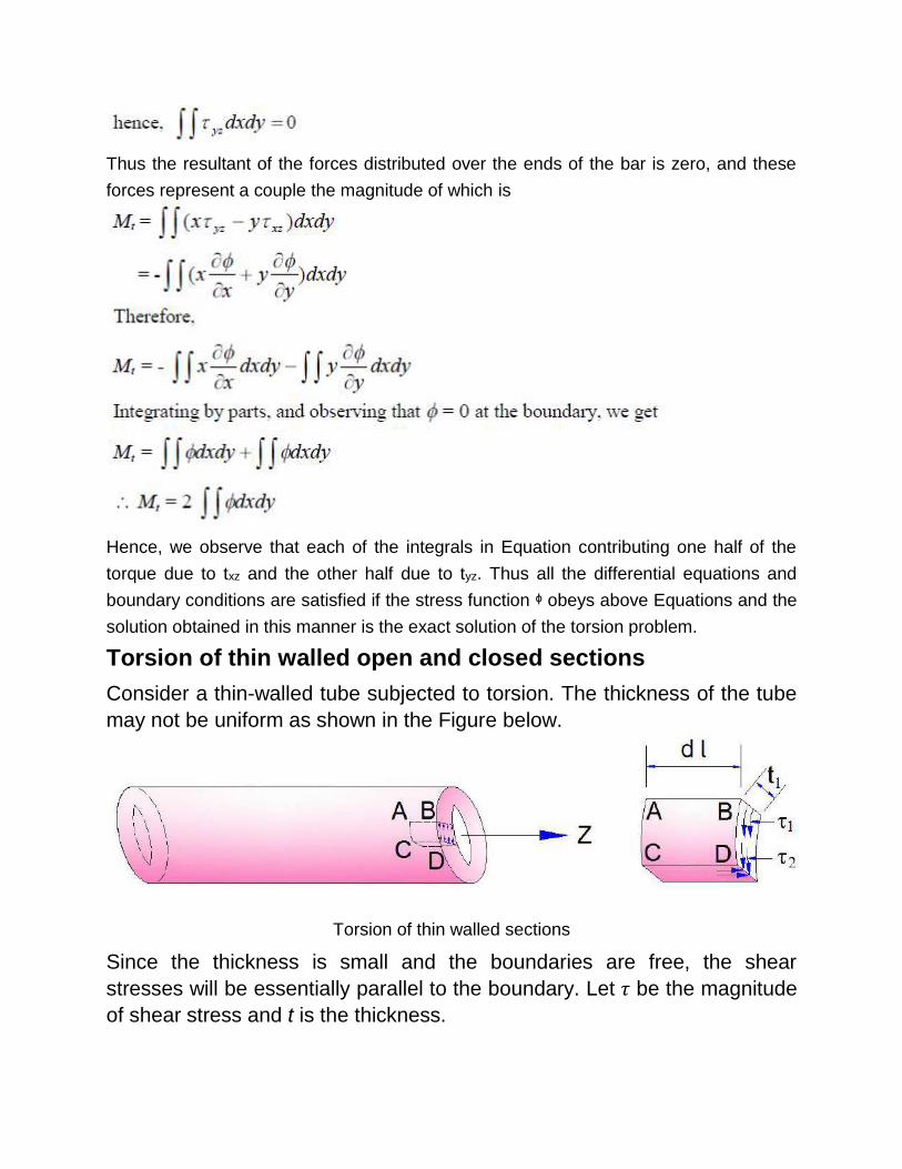
Torsion of thin walled open and closed sections
Consider a thin-walled tube subjected to torsion. The thickness of the tube
may not be uniform as shown in the Figure below.
Torsion of thin walled sections
Since the thickness is small and the boundaries are free, the shear
stresses will be essentially parallel to the boundary. Let 𝜏 be the magnitude
of shear stress and t is the thickness.

Now, consider the equilibrium of an element of length D l as shown in
Figure below. The areas of cut faces AB and CD are t1 D l and t2 D l
respectively. The shear stresses (complementary shears) are t1 and t2.
Determination of Torque due to shear and Rotation:
Cross section of a thin-walled tube and torque due to shear
Consider the torque of the shear about point O
Where A is the area enclosed by the centre line of the tube

To determine the twist of the tube
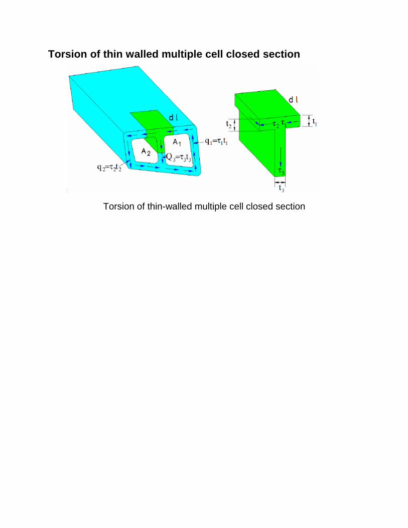
Torsion of thin walled multiple cell closed section
Torsion of thin-walled multiple cell closed section

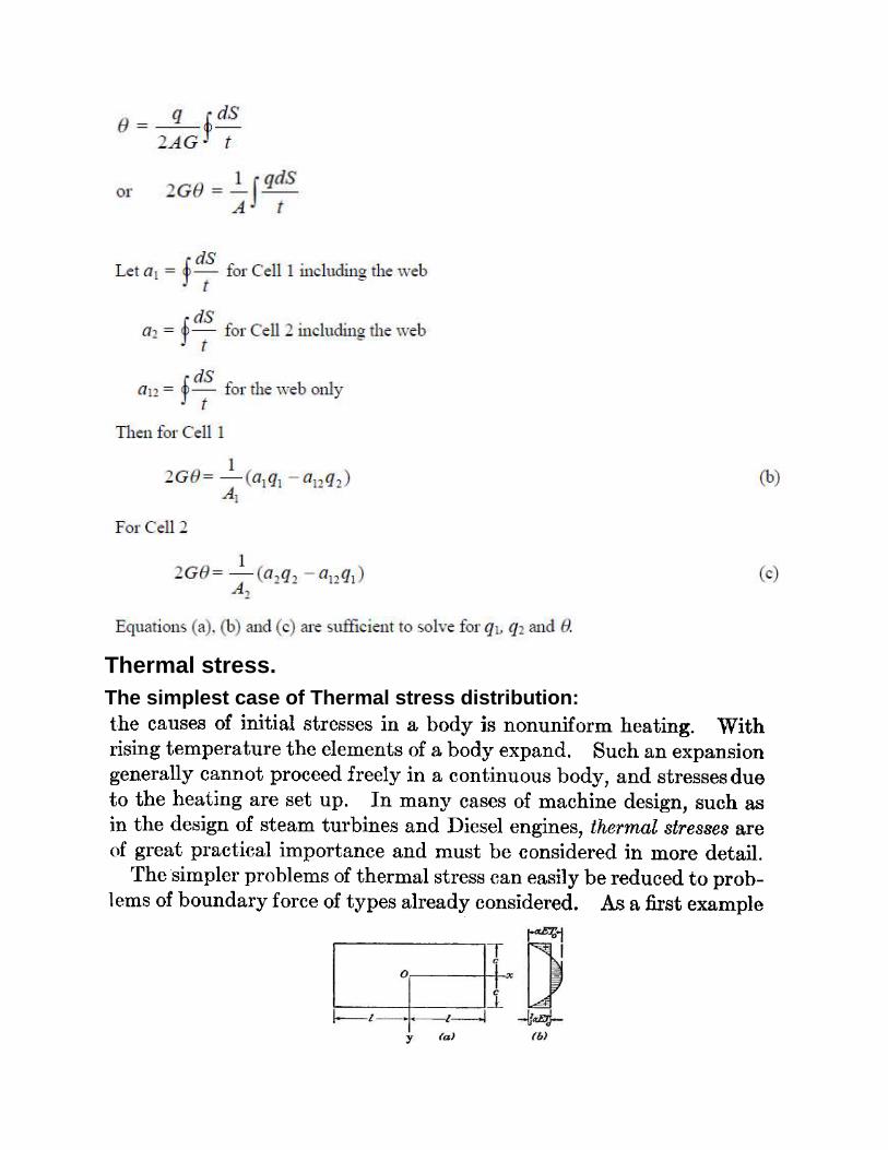
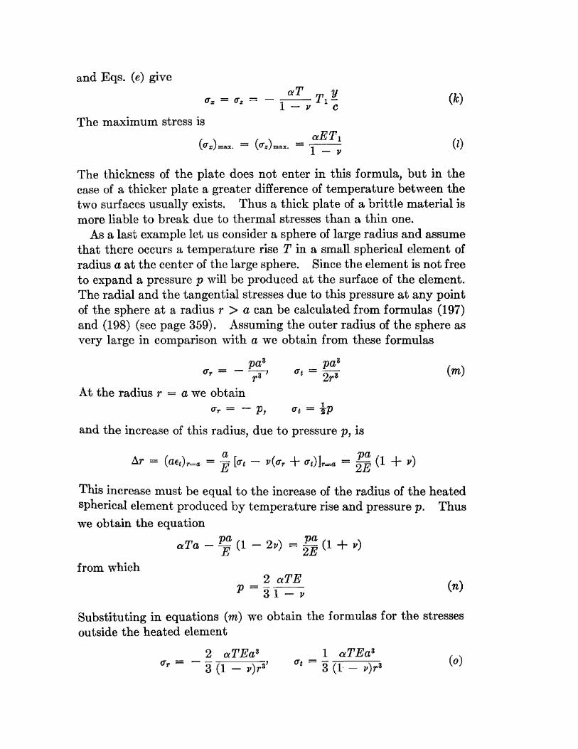
Thermal stress.
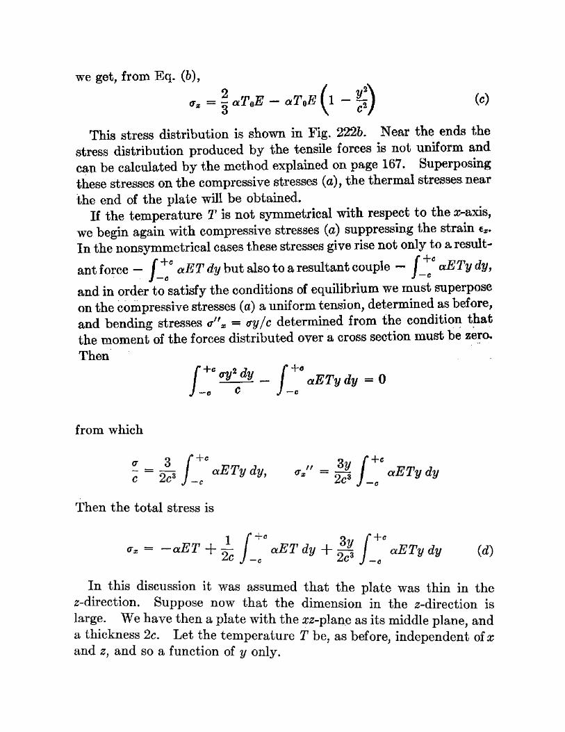
The simplest case of Thermal stress distribution:


Module-IV
Theoretical concepts of plasticity
The classical theory of plasticity grew out of the study of metals in the
late nineteenth century. It is concerned with materials which initially deform
elastically, but which deform plastically upon reaching a yield stress. In
metals and other crystalline materials the occurrence of plastic
deformations at the micro-scale level is due to the motion of dislocations
and the migration of grain boundaries on the micro-level. In sands and
other granular materials plastic flow is due both to the irreversible
rearrangement of individual particles and to the irreversible crushing of
individual particles. Similarly, compression of bone to high stress levels will
lead to particle crushing. The deformation of microvoids and the
development of micro-cracks is also an important cause of plastic
deformations in materials such as rocks.
A good part of the discussion in what follows is concerned with the
plasticity of metals; this is the ‘simplest’ type of plasticity and it serves as a
good background and introduction to the modelling of plasticity in other
material-types. There are two broad groups of metal plasticity problem
which are of interest to the engineer and analyst. The first involves
relatively small plastic strains, often of the same order as the elastic strains
which occur. Analysis of problems involving small plastic strains allows one
to design structures optimally, so that they will not fail when in service, but
at the same time are not stronger than they really need to be. In this sense,
plasticity is seen as a material failure1.
The second type of problem involves very large strains and deformations,
so large that the elastic strains can be disregarded. These problems occur
in the analysis of metals manufacturing and forming processes, which can
involve extrusion, drawing, forging, rolling and so on. In these latter-type
problems, a simplified model known as perfect plasticity is usually
employed (see below), and use is made of special limit theorems which
hold for such models.
Plastic deformations are normally rate independent, that is, the stresses
induced are independent of the rate of deformation (or rate of loading). This
is in marked contrast to classical Newtonian fluids for example, where the
stress levels are governed by the rate of deformation through the viscosity
of the fluid.
Materials commonly known as “plastics” are not plastic in the sense
described here. They, like other polymeric materials, exhibit viscoelastic
behaviour where, as the name suggests, the material response has both
elastic and viscous components. Due to their viscosity, their response is,
unlike the plastic materials, rate-dependent. Further, although the
viscoelastic materials can suffer irrecoverable deformation, they do not
have any critical yield or threshold stress, which is the characteristic
property of plastic behaviour. When a material undergoes plastic
deformations, i.e. irrecoverable and at a critical yield stress, and these
effects are rate dependent, the material is referred to as being viscoplastic.
Plasticity theory began with Tresca in 1864, when he undertook an
experimental program into the extrusion of metals and published his
famous yield criterion discussed later on. Further advances with yield
criteria and plastic flow rules were made in the years which followed by
Saint-Venant, Levy, Von Mises, Hencky and Prandtl. The 1940s saw the
advent of the classical theory; Prager, Hill, Drucker and Koiter amongst
others brought together many fundamental aspects of the theory into a
single framework. The arrival of powerful computers in the 1980s and
1990s provided the impetus to develop the theory further, giving it a more
rigorous foundation based on thermodynamics principles, and brought with
it the need to consider many numerical and computational aspects to the
plasticity problem.
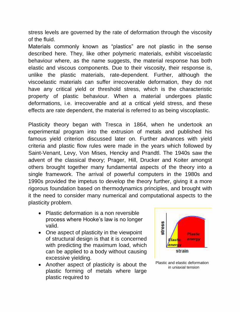
Plastic and elastic deformation
in uniaxial tension
Plastic deformation is a non reversible process where Hooke’s law is no longer valid.
One aspect of plasticity in the viewpoint of structural design is that it is concerned with predicting the maximum load, which can be applied to a body without causing excessive yielding.
Another aspect of plasticity is about the plastic forming of metals where large plastic required to
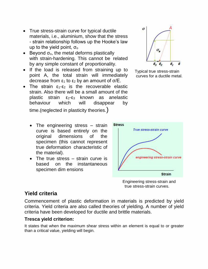
Typical true stress-strain curves for a ductile metal.
Engineering stress-strain and true stress-strain curves.
Yield criteria
Commencement of plastic deformation in materials is predicted by yield criteria. Yield criteria are also called theories of yielding. A number of yield criteria have been developed for ductile and brittle materials.
Tresca yield criterion:
It states that when the maximum shear stress within an element is equal to or greater than a critical value, yielding will begin.
True stress-strain curve for typical ductile materials, i.e., aluminium, show that the stress - strain relationship follows up the Hooke’s law up to the yield point, σo.
Beyond σo, the metal deforms plastically with strain-hardening. This cannot be related by any simple constant of proportionality.
If the load is released from straining up to point A, the total strain will immediately decrease from ε1 to ε2 by an amount of σ/E.
The strain ε1-ε2 is the recoverable elastic strain. Also there will be a small amount of the plastic strain ε2-ε3 known as anelastic behaviour which will disappear by
time.(neglected in plasticity theories.)
The engineering stress – strain curve is based entirely on the original dimensions of the specimen (this cannot represent true deformation characteristic of the material).
The true stress – strain curve is based on the instantaneous specimen dim ensions
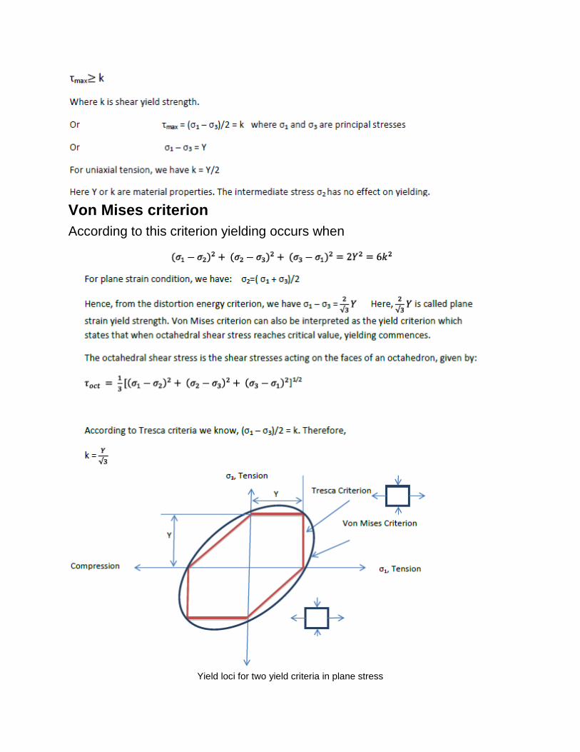
Von Mises criterion
According to this criterion yielding occurs when
Yield loci for two yield criteria in plane stress
Von Mises yield criterion is found to be suitable for most of the ductile
materials used in forming operations. More often in metal forming, this
criterion is used for the analysis. The suitability of the yield criteria has
been experimentally verified by conducting torsion test on thin walled tube,
as the thin walled tube ensures plane stress. However, the use of Tresca
criterion is found to result in negligible difference between the two criteria.
We observe that the von Mises criterion is able to predict the yielding
independent of the sign of the stresses because this criterion has square
terms of the shear stresses.
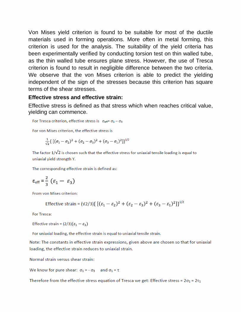
Effective stress and effective strain:
Effective stress is defined as that stress which when reaches critical value, yielding can commence.

Similarly using von Mises effective stress, we have
A plane strain compression forging process
Plastic stress strain relationship,
Elastic plastic problems in bending and torsion.