LECTURE NOTES ON DIFFERENTIABLE …...LECTURE NOTES ON DIFFERENTIABLE MANIFOLDS JIE WU Contents 1....

LECTURE NOTES ON DIFFERENTIABLE MANIFOLDS

JIE WU

Contents

1. Tangent Spaces, Vector Fields in Rn and the Inverse Mapping Theorem 21.1. Tangent Space to a Level Surface 21.2. Tangent Space and Vectors Fields on Rn 31.3. Operator Representations of Vector Fields 31.4. Integral Curves 51.5. Implicit- and Inverse-Mapping Theorems 62. Topological and Differentiable Manifolds, Diffeomorphisms, Immersions, Submersions

and Submanifolds 102.1. Topological Spaces 102.2. Topological Manifolds 102.3. Differentiable Manifolds 122.4. Tangent Space 132.5. Immersions 152.6. Submersions 173. Examples of Manifolds 193.1. Open Stiefel Manifolds and Grassmann Manifolds 193.2. Stiefel Manifold 214. Fibre Bundles and Vector Bundles 224.1. Fibre Bundles 224.2. G-Spaces and Principal G-Bundles 254.3. The Associated Principal G-Bundles of Fibre Bundles 274.4. Vector Bundles 314.5. The Construction of Gauss Maps 315. Tangent Bundles and Vector Fields 375.1. Tangent Bundles 375.2. Vector Fields 395.3. Vector Fields on Spheres 446. Riemann Metric and Cotangent Bundles 456.1. Riemann and Hermitian Metrics on Vector Bundles 456.2. Constructing New Bundles Out of Old and Cotangent Bundle 486.3. Cotangent Bundles and Co-vector Fields 507. Tensor Bundles, Tensor Fields and Differential Forms 517.1. Tensor Product 517.2. Tensor Algebras 547.3. Graded Modules, Graded Commutative Algebras and Exterior Algebras 56

1

2 JIE WU

7.4. Tensor Bundles, Tensor Fields 607.5. Differential Forms 608. Orientation and Integration 618.1. Alternating Multi-linear Functions and Forms 618.2. Orientation of Manifolds 668.3. Integration of m-forms on Oriented m-Manifolds 709. The Exterior Derivative and the Stokes Theorem 719.1. Exterior Derivative on Rm 719.2. Exterior Derivative on Manifolds 739.3. Stokes’ Theorem 74References 78

1. Tangent Spaces, Vector Fields in Rn and the Inverse Mapping Theorem

1.1. Tangent Space to a Level Surface. Let γ be a curve in Rn: γ : t 7→ (γ1(t), γ2(t), . . . , γn(t)).(A curve can be described as a vector-valued function. Converse a vector-valued function gives acurve in Rn.) The tangent line at the point γ(t0) is given with the direction

dγ

dt(t0) =

(dγ1

dt(t0), . . . ,

dγn

t(t0)

).

(Certainly we need to assume that the derivatives exist. We may talk about smooth curves, that is,the curves with all continuous higher derivatives.)

Consider the level surface f(x1, x2, . . . , xn) = c of a differentiable function f , where xi refers toi-th coordinate. The gradient vector of f at a point P = (x1(P ), x2(P ), . . . , xn(P )) is

∇f = (∂f

∂x1, . . . ,

∂f

∂xn).

Given a vector ~u = (u1, . . . , un), the directional derivative is

D~uf = ∇f · ~u =∂f

∂x1u1 + · · ·+ ∂f

∂xnun.

The tangent space at the point P on the level surface f(x1, . . . , xn) = c is the (n − 1)-dimensional(if ∇f 6= 0) space through P normal to the gradient ∇f . In other words, the tangent space is givenby the equation

∂f

∂x1(P )(x1 − x1(P )) + · · ·+ ∂f

∂xn(P )(xn − xn(P )) = 0.

From the geometric views, the tangent space should consist of all tangents to the smooth curveson the level surface through the point P . Assume that γ is a curve through P (when t = t0)that lies in the level surface f(x1, . . . , xn) = c, that is

f(γ1(t), γ2(t), . . . , γn(t)) = c.

By taking derivatives on both sides,∂f

∂x1(P )(γ1)′(t0) + · · ·+ ∂f

∂xn(P )(γn)′(t0) = 0

and so the tangent line of γ is really normal (orthogonal) to ∇f . When γ runs over all possiblecurves on the level surface through the point P , then we obtain the tangent space at the point P .

LECTURE NOTES ON DIFFERENTIABLE MANIFOLDS 3

Roughly speaking, a tangent space is a vector space attached to a point in the surface.How to obtain the tangent space: take all tangent lines of smooth curve through this point on the

surface.

1.2. Tangent Space and Vectors Fields on Rn. Now consider the tangent space of Rn. Accord-ing to the ideas in the previous subsection, first we assume a given point P ∈ Rn. Then we considerall smooth curves passes through P and then take the tangent lines from the smooth curves. Theobtained vector space at the point P is the n-dimensional space. But we can look at in a littledetail.

Let γ be a smooth curve through P . We may assume that γ(0) = P . Let ω be another smoothcurve with ω(0) = P . γ is called to be equivalent to ω if the directives γ′(0) = ω′(0). The tangentspace of Rn at P , denoted by TP (Rn), is then the set of equivalence class of all smooth curvesthrough P .

Let T (Rn) =⋃

P∈Rn

TP (Rn), called the tangent bundle of Rn. If S is a region of Rn, let T (S) =⋃P∈S

TP (S), called the tangent bundle of S.

Note. Each TP (Rn) is an n-dimensional vector space, but T (S) is not a vector space. In otherwords, T (S) is obtained by attaching a vector space TP (Rn) to each point P in S. Also S is assumedto be a region of Rn, otherwise the tangent space of S (for instance S is a level surface) could be aproper subspace of TP (Rn).

If γ is a smooth curve from P to Q in Rn, then the tangent space TP (Rn) moves along γ toTQ(Rn). The direction for this moving is given γ′(t), which introduces the following importantconcept.

Definition 1.1. A vector field V on a region S of Rn is a smooth map (also called C∞-map)

V : S → T (S) P 7→ ~v(P ).

Let V : P 7→ ~v(P ) and W : P 7→ ~w(P ) be two vector fields and let f : S → R be a smoothfunction. Then V +W : P 7→ ~v(P ) + ~w(P ) and fV : P 7→ f(P )~v(P ) give (pointwise) addition andscalar multiplication structure on vector fields.

1.3. Operator Representations of Vector Fields. Let J be an open interval containing 0 andlet γ : J → Rn be a smooth curve with γ(0) = P . Let f = f(x1, . . . , xn) be a smooth functiondefined on a neighborhood of P . Assume that the range of γ is contained in the domain of f . Byapplying the chain rule to the composite T = f γ : J → R,

Dγ(f) :=dT

dt=

n∑i=1

dγi(t)dt

∂f

∂xi

∣∣∣∣∣xi=γi(t)

Proposition 1.2.

Dγ(af + bg) = aDγ(f) + bDγ(g), where a, b are constant.

Dγ(fg) = Dγ(f)g + fDγ(g).

Let C∞(Rn) denote the set of smooth functions on Rn. An operation D on C∞(Rn) is called aderivation if D maps C∞(Rn) to C∞(Rn) and satisfies the conditions

D(af + bg) = aD(f) + bD(g), where a, b are constant.

4 JIE WU

D(fg) = D(f)g + fD(g).

Example: For 1 ≤ i ≤ n,

∂i : f 7→∂f

∂xi

is a derivation.

Proposition 1.3. Let D be any derivation on C∞(Rn). Given any point P in Rn. Then thereexist real numbers a1, a2, . . . , an ∈ R such that

D(f)(P ) =n∑i=1

ai∂i(f)(P )

for any f ∈ C∞(Rn), where ai depends on D and P but is independent on f .

Proof. Write x for (x1, . . . , xn). Define

gi(x) =∫ 1

0

∂f

∂xi(t(x− P ) + P )dt.

Then

f(x)− f(P ) =∫ 1

0

d

dtf(t(x− P ) + P )dt

=∫ 1

0

n∑i=1

∂f

∂xi(t(x− P ) + P ) · (xi − xi(P ))dt

=n∑i=1

(xi − xi(P ))∫ 1

0

∂f

∂xi(t(x− P ) + P )dt =

n∑i=1

(xi − xi(P ))gi(x).

Since D is a derivation, D(1) = D(1 · 1) = D(1) · 1 + 1 · D(1) and so D(1) = 0. It follows thatD(c) = 0 for any constant c. By applying D to the above equations,

D(f(x)) = D(f(x)− f(P )) =n∑i=1

D(xi − xi(P ))gi(x) + (xi − xi(P ))D(gi(x))

=n∑i=1

D(xi)gi(x) + (xi − xi(P ))D(gi(x))

because D(f(P )) = D(xi(P )) = 0. Let ai = D(xi)(P ) which only depends on D and P . Byevaluating at P ,

D(f)(P ) =n∑i=1

D(xi)(P )gi(P ) + 0 =n∑i=1

aigi(P ).

Since

gi(P ) =∫ 1

0

∂f

∂xi(t(P − P ) + P )dt =

∫ 1

0

∂f

∂xi(P )dt =

∂f

∂xi(P ) = ∂i(f)(P ),

D(f)(P ) =n∑i=1

ai∂i(f)(P ),

which is the conclusion.


From this proposition, we can give a new way to looking at vector fields:Given a vector fields P 7→ ~v(P ) = (v1(P ), v2(P ), . . . , vn(P )), a derivation

D~v =n∑i=1

vi(P ) · ∂i

on C∞(Rn) is called an operator representation of the vector field P 7→ ~v(P ).Note. The operation vi(x)∂i is given as follows: for any f ∈ C∞(Rn),

D~v(f)(P ) =n∑i=1

vi(P ) · ∂i(f)(P )

for any P .From this new view, the tangent spaces T (Rn) admits a basis ∂1, ∂2, . . . , ∂n.

1.4. Integral Curves. Let V : x 7→ ~v(x) be a (smooth) vector field on an neighborhood U of P .An integral curve to V is a smooth curve s : (−δ, ε) → U , defined for suitable δ, ε > 0, such that

s′(t) = ~v(s(t))

for −δ < t < ε.

Theorem 1.4. Let V : x 7→ ~v(x) be a (smooth) vector field on an neighborhood U of P . Then thereexists an integral curve to V through P . Any two such curves agree on their common domain.

Proof. The proof is given by assuming the fundamental existence and uniqueness theorem for sys-tems of first order differential equations.

The requirement for a curve s(t) = (s1(t), . . . , sn(t)) to be an integral curve is:ds1(t)dt = v1(s1(t), s2(t), . . . , sn(t))

ds2(t)dt = v2(s1(t), s2(t), . . . , sn(t))

· · · · · · · · ·dsn(t)dt = vn(s1(t), s2(t), . . . , sn(t))

with the initial conditions

s(0) = P (s1(0), s2(0), . . . , sn(0)) = (x1(P ), x2(P ), . . . , xn(P ))

s′(0) = ~v(P )(ds1

dt(0), . . . ,

dsn

dt(0))

= (v1(P ), . . . , vn(P )).

Thus the statement follows from the fundamental theorem of first order ODE.

Example 1.5. Let n = 2 and let V : P 7→ ~v(P ) = (v1(P ), v2(P )), where v1(x, y) = x and v2(x, y) =y. Given a point P = (a1, a2), the equation for the integral curve s(t) = (x(t), y(t)) is

x′(t) = v1(s(t)) = x(t)y′(t) = v2(s(t)) = y(t)

with initial conditions (x(0), y(0)) = (a1, a2) and (x′(0), y′(0)) = ~v(a1, a2) = (a1, a2). Thus thesolution is

s(t) = (a1et, a2et).

6 JIE WU

Example 1.6. Let n = 2 and let V : P 7→ ~v(P ) = (v1(P ), v2(P )), where v1(x, y) = x and v2(x, y) =−y. Given a point P = (a1, a2), the equation for the integral curve s(t) = (x(t), y(t)) is

x′(t) = v1(s(t)) = x(t)y′(t) = v2(s(t)) = −y(t)

with initial conditions (x(0), y(0)) = (a1, a2) and (x′(0), y′(0)) = ~v(a1, a2) = (a1,−a2). Thus thesolution is

s(t) = (a1et, a2e−t).

1.5. Implicit- and Inverse-Mapping Theorems.

Theorem 1.7. Let D be an open region in Rn+1 and let F be a function well-defined on D withcontinuous partial derivatives. Let (x1

0, x20, . . . , x

n0 , z0) be a point in D where

F (x10, x

20, . . . , x

n0 , z0) = 0

∂F

∂z(x1

0, x20, . . . , x

n0 , z0) 6= 0.

Then there is a neighborhood Nε(z0) ⊆ R, a neighborhood Nδ(x10, . . . , x

n0 ) ⊆ Rn, and a unique

function z = g(x1, x2, . . . , xn) defined for (x1, . . . , xn) ∈ Nδ(x10, . . . , x

n0 ) with values z ∈ Nε(z0) such

that1) z0 = g(x1

0, x20, . . . , x

n0 ) and

F (x1, x2, . . . , xn, g(x1, . . . , xn)) = 0

for all (x1, . . . , xn) ∈ Nδ(x10, . . . , x

n0 ).

2) g has continuous partial derivatives with

∂g

∂xi(x1, . . . , xn) = −Fx

i(x1, . . . , xn, z)Fz(x1, . . . , xn, z)

for all (x1, . . . , xn) ∈ Nδ(x10, . . . , x

n0 ) where z = g(x1, . . . , xn).

3) If F is smooth on D, then z = g(x1, . . . , xn) is smooth on Nδ(x10, . . . , x

n0 ).

Proof. Step 1. We may assume that ∂F∂z (x1

0, x20, . . . , x

n0 , z0) > 0. Since Fz is continuous, there

exists a neighborhood Nε(x10, x

20, . . . , x

n0 , z0) in which Fz is continuous and positive. Thus for fixed

(x1, . . . , xn), F is strictly increasing on z in this neighborhood. It follows that there exists c > 0such that

F (x10, x

20, . . . , x

n0 , z0 − c) < 0 F (x1

0, x20, . . . , x

n0 , z0 + c) > 0

with(x1

0, x20, . . . , x

n0 , z0 − c), (x1

0, x20, . . . , x

n0 , z0 + c) ∈ Nε(x1

0, x20, . . . , x

n0 , z0).

Step 2. By the continuity of F , there exists a small δ > 0 such that

F (x1, x2, . . . , xn, z0 − c) < 0 F (x1, x2, . . . , xn, z0 + c) > 0

with(x1, x2, . . . , xn, z0 − c), (x1, x2, . . . , xn, z0 + c) ∈ Nε(x1

0, x20, . . . , x

n0 , z0)

for (x1, . . . , xn) ∈ Nδ(x10, . . . , x

n0 ).

Step 3. Fixed (x1, . . . , xn) ∈ Nδ(x10, . . . , x

n0 ), F is continuous and strictly increasing on z. There is

a unique z, z0 − c < z < z0 + c, such that

F (x1, . . . , xn, z) = 0.


This defines a function z = g(x1, . . . , xn) for (x1, . . . , xn) ∈ Nδ(x10, . . . , x

n0 ) with values z ∈ (z0 −

c, z0 + c).Step 4. Prove that z = g(x1, . . . , xn) is continuous. Let (x1

1, . . . , xn1 ) ∈ Nδ(x1

0, . . . , xn0 ). Let

(x11(k), . . . , x

n1 (k)) be any sequence in Nδ(x1

0, . . . , xn0 ) converging to (x1

1, . . . , xn1 ). Let A be any

subsequential limit of zk = g(x11(k), . . . , x

n1 (k)), that is A = lim

s→∞zks

. Then, by the continuity ofF ,

0 = lims→∞

F (x11(ks), . . . , x

n1 (ks), zks

)

= F ( lims→∞

x11(ks), . . . , lim

s→∞xn1 (ks), lim

s→∞zks

)

= F (x11, . . . , x

n1 , A).

By the unique solution of the equation, A = g(x11, . . . , x

n1 ). Thus zk converges g(x1

1, . . . , xn1 ) and

so g is continuous.Step 5. Compute the partial derivatives ∂z

∂xi. Let h be small enough. Let

z + k = g(x1, . . . , xi−1, xi + h, xi+1, . . . , xn),

that isF (x1, . . . , xi + h, . . . , xn, z + k) = 0

with z0 − c < z + k < z0 + c. Then

0 = F (x1, . . . , xi + h, . . . , xn, z + k)− F (x1, . . . , xn, z)

= Fxi(x1, . . . , xi, . . . , xn, z)h+ Fz(x1, . . . , xi, . . . , xn, z)kby the mean value theorem (Consider the function

φ(t) = F (x1, . . . , xi + th, . . . , xn, z + tk)

for 0 ≤ t ≤ 1. Then φ(1)−φ(0) = φ′(ξ)(1−0).), where xi is between xi and xi+h, and z is betweenz and z + k. Now

∂g

∂xi= limh→0

g(x1, . . . , xi−1, xi + h, xi+1, . . . , xn)− z

h= limh→0

k

h

= − limh→0

Fxi(x1, . . . , xi, . . . , xn, z)Fz(x1, . . . , xi, . . . , xn, z)

. = −Fxi

Fz,

where z → z as h→ 0 because g is continuous (and so k → 0 as h→ 0).Step 6. Since Fz is not zero in this small neighborhood, gxi

is continuous for each i. If F is smooth,then all higher derivatives of g are continuous and so g is also smooth.

Theorem 1.8 (Implicit Function Theorem). Let D be an open region in Rm+n and let F1, F2, . . . , Fnbe functions well-defined on D with continuous partial derivatives. Let (x1

0, x20, . . . , x

m0 , u

10, u

20, . . . , u

n0 )

be a point in D where F1(x1

0, x20, . . . , x

m0 , u

10, u

20, . . . , u

n0 ) = 0

F2(x10, x

20, . . . , x

m0 , u

10, u

20, . . . , u

n0 ) = 0

· · · · · · · · · · · ·Fn(x1

0, x20, . . . , x

m0 , u

10, u

20, . . . , u

n0 ) = 0

and the Jacobian

J =∂(F1, F2, . . . , Fn)∂(u1, u2, . . . , un)

= det(∂Fi∂uj

)6= 0

8 JIE WU

at the point (x10, x

20, . . . , x

m0 , u

10, u

20, . . . , u

n0 ). Then there are neighborhoods Nδ(x1

0, . . . , xm0 ), Nε1(u

10),

Nε2(u20), . . ., Nεn(un0 ), and unique functions

u1 = g1(x1, x2, . . . , xm)u2 = g2(x1, x2, . . . , xm)

· · · · · · · · · · · ·un = gn(x1, x2, . . . , xm)

defined for (x1, . . . , xm) ∈ Nδ(x10, . . . , x

m0 ) with values u1 ∈ Nε1(u1

0), . . . , un ∈ Nεn(un0 ) such that

1) ui0 = gi(x10, x

20, . . . , x

m0 ) and

Fi(x1, x2, . . . , xn, gi(x1, . . . , xm)) = 0

for all 1 ≤ i ≤ n and all (x1, . . . , xm) ∈ Nδ(x10, . . . , x

m0 ).

2) Each gi has continuous partial derivatives with

∂gi∂xj

(x1, . . . , xm) = − 1J· ∂(F1, . . . , Fn)∂(u1, u2, . . . , uj−1, xj , uj+1, . . . , un)

for all (x1, . . . , xm) ∈ Nδ(x10, . . . , x

m0 ) where ui = gi(x1, . . . , xm).

3) If each Fi is smooth on D, then each ui = gi(x1, . . . , xm) is smooth on Nδ(x10, . . . , x

m0 ).

Sketch of Proof. The proof is given by induction on n. Assume that the statement holds for n− 1with n > 1. (We already prove that the statement holds for n = 1.) Since the matrix(

∂Fi∂uj

)is invertible at the point P = (x1

0, x20, . . . , x

m0 , u

10, u

20, . . . , u

n0 ) (because the determinant is not zero),

we may assume that∂Fn∂un

(P ) 6= 0.

(The entries in the last column can not be all 0 and so, if ∂Fi

∂un (P ) 6= 0, we can interchange Fi andFn.)

From the previous theorem, there is a solution

un = gn(x1, . . . , xm, u1, . . . , un−1)

to the last equation. ConsiderG1 = F1(x1, . . . , xm, u1, . . . , un−1, gn)G2 = F2(x1, . . . , xm, u1, . . . , un−1, gn)

· · · · · · · · · · · ·Gn−1 = Fn−1(x1, . . . , xm, u1, . . . , un−1, gn).

Then∂Gi∂uj

=∂Fi∂uj

+∂Fi∂un

· ∂gn∂uj

for 1 ≤ i, j ≤ n− 1, where∂Fn∂uj

+∂Fn∂un

· ∂gn∂uj

= 0.


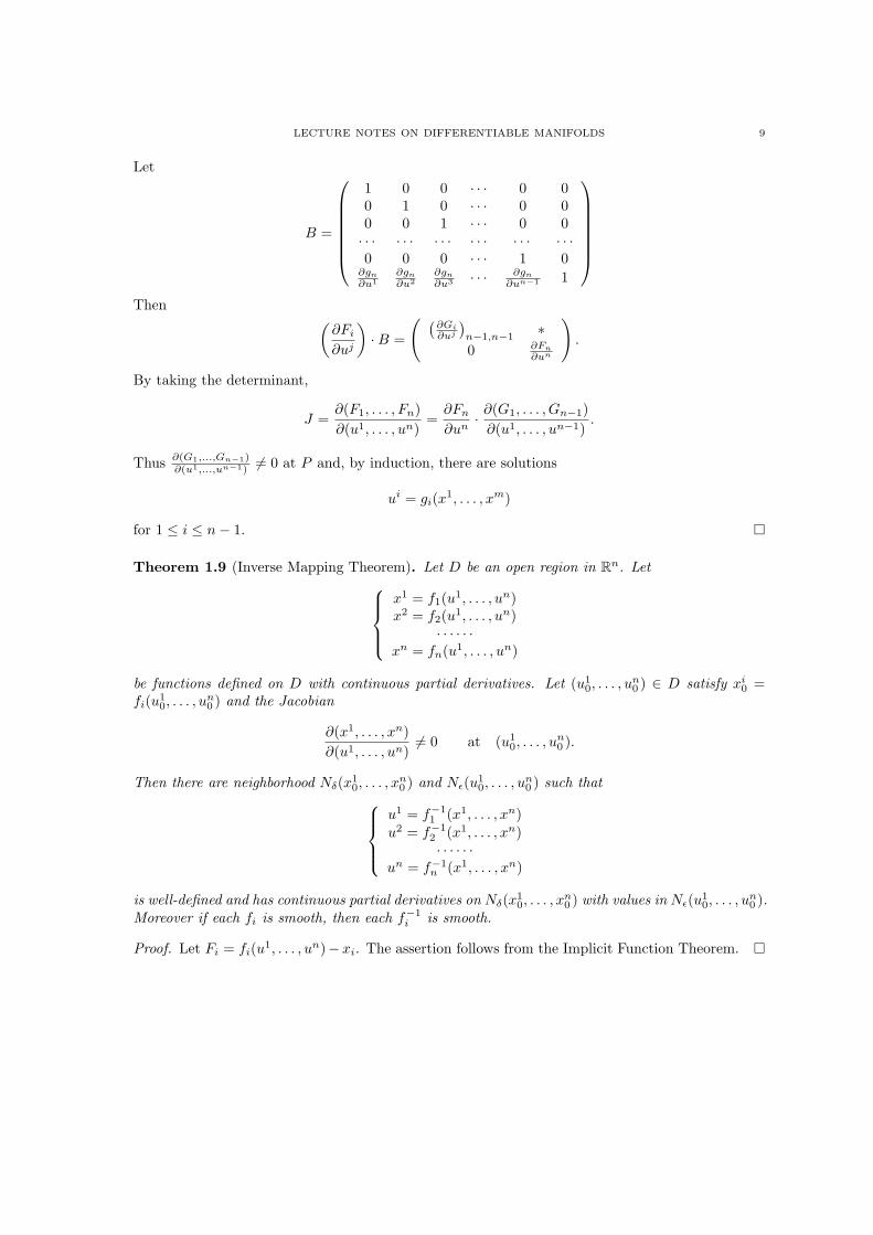
Let

B =

1 0 0 · · · 0 00 1 0 · · · 0 00 0 1 · · · 0 0· · · · · · · · · · · · · · · · · ·0 0 0 · · · 1 0∂gn

∂u1∂gn

∂u2∂gn

∂u3 · · · ∂gn

∂un−1 1

Then (

∂Fi∂uj

)·B =

( (∂Gi

∂uj

)n−1,n−1

∗0 ∂Fn

∂un

).

By taking the determinant,

J =∂(F1, . . . , Fn)∂(u1, . . . , un)

=∂Fn∂un

· ∂(G1, . . . , Gn−1)∂(u1, . . . , un−1)

.

Thus ∂(G1,...,Gn−1)∂(u1,...,un−1) 6= 0 at P and, by induction, there are solutions

ui = gi(x1, . . . , xm)

for 1 ≤ i ≤ n− 1.

Theorem 1.9 (Inverse Mapping Theorem). Let D be an open region in Rn. Letx1 = f1(u1, . . . , un)x2 = f2(u1, . . . , un)

· · · · · ·xn = fn(u1, . . . , un)

be functions defined on D with continuous partial derivatives. Let (u10, . . . , u

n0 ) ∈ D satisfy xi0 =

fi(u10, . . . , u

n0 ) and the Jacobian

∂(x1, . . . , xn)∂(u1, . . . , un)

6= 0 at (u10, . . . , u

n0 ).

Then there are neighborhood Nδ(x10, . . . , x

n0 ) and Nε(u1

0, . . . , un0 ) such that

u1 = f−11 (x1, . . . , xn)

u2 = f−12 (x1, . . . , xn)· · · · · ·

un = f−1n (x1, . . . , xn)

is well-defined and has continuous partial derivatives on Nδ(x10, . . . , x

n0 ) with values in Nε(u1

0, . . . , un0 ).

Moreover if each fi is smooth, then each f−1i is smooth.

Proof. Let Fi = fi(u1, . . . , un)−xi. The assertion follows from the Implicit Function Theorem.

10 JIE WU

2. Topological and Differentiable Manifolds, Diffeomorphisms, Immersions,Submersions and Submanifolds

2.1. Topological Spaces.

Definition 2.1. Let X be a set. A topology U for X is a collection of subsets of X satisfyingi) ∅ and X are in U ;ii) the intersection of two members of U is in U ;iii) the union of any number of members of U is in U .

The set X with U is called a topological space. The members U ∈ U are called the open sets.

Let X be a topological space. A subset N ⊆ X with x ∈ N is called a neighborhood of x if thereis an open set U with x ∈ U ⊆ N . For example, if X is a metric space, then the closed ball Dε(x)and the open ball Bε(x) are neighborhoods of x. A subset C is said to closed if X \ C is open.

Definition 2.2. A function f : X → Y between two topological spaces is said to be continuous iffor every open set U of Y the pre-image f−1(U) is open in X.

A continuous function from a topological space to a topological space is often simply called amap. A space means a Hausdorff space, that is, a topological spaces where any two points hasdisjoint neighborhoods.

Definition 2.3. Let X and Y be topological spaces. We say that X and Y are homeomorphic ifthere exist continuous functions f : X → Y, g : Y → X such that f g = idY and g f = idX . Wewrite X ∼= Y and say that f and g are homeomorphisms between X and Y .

By the definition, a function f : X → Y is a homeomorphism if and only ifi) f is a bijective;ii) f is continuous andiii) f−1 is also continuous.

Equivalently f is a homeomorphism if and only if 1) f is a bijective, 2) f is continuous and 3) f isan open map, that is f sends open sets to open sets. Thus a homeomorphism between X and Y isa bijective between the points and the open sets of X and Y .

A very general question in topology is how to classify topological spaces under homeomorphisms.For example, we know (from complex analysis and others) that any simple closed loop is homeo-morphic to the unit circle S1. Roughly speaking topological classification of curves is known. Thetopological classification of (two-dimensional) surfaces is known as well. However the topologicalclassification of 3-dimensional manifolds (we will learn manifolds later.) is quite open.

The famous Poicare conjecture is related to this problem, which states that any simply connected3-dimensional (topological) manifold is homeomorphic to the 3-sphere S3. A spaceX is called simplyconnected if (1) X is path-connected (that is, given any two points, there is a continuous path joiningthem) and (2) the fundamental group π1(X) is trivial (roughly speaking, any loop can be deformedto be the constant loop in X). The manifolds are the objects that we are going to discuss in thiscourse.

2.2. Topological Manifolds. A Hausdorff space M is called a (topological) n-manifold if eachpoint of M has a neighborhood homeomorphic to an open set in Rn. Roughly speaking, an n-manifold is locally Rn. Sometimes M is denoted as Mn for mentioning the dimension of M .


(Note. If you are not familiar with topological spaces, you just think that M is a subspace ofRN for a large N .)

For example, Rn and the n-sphere Sn is an n-manifold. A 2-dimensional manifold is calleda surface. The objects traditionally called ‘surfaces in 3-space’ can be made into manifolds ina standard way. The compact surfaces have been classified as spheres or projective planes withvarious numbers of handles attached.

By the definition of manifold, the closed n-disk Dn is not an n-manifold because it has the‘boundary’ Sn−1. Dn is an example of ‘manifolds with boundary’. We give the definition ofmanifold with boundary as follows.

A Hausdorff space M is called an n-manifold with boundary (n ≥ 1) if each point in M has aneighborhood homeomorphic to an open set in the half space

Rn+ = (x1, · · · , xn) ∈ Rn|xn ≥ 0.Manifold is one of models that we can do calculus ‘locally’. By means of calculus, we need local

coordinate systems. Let x ∈M . By the definition, there is a an open neighborhood U(x) of x anda homeomorphism φx from U(x) onto an open set in Rn+. The collection (U(x), φx)|x ∈ M hasthe property that 1) U(x)|x ∈ M is an open cover and 2) φx is a homeomorphism from U(x)onto an open set in Rn+. The subspace φx(Ux) in Rn+ plays a role as a local coordinate system. Thecollection (U(x), φx)|x ∈M is somewhat too large and we may like less local coordinate systems.This can be done as follows.

Let M be a space. A chart of M is a pair (U, φ) such that 1) U is an open set in M and 2) φ isa homeomorphism from U onto an open set in Rn+. The map

φ : U → Rn+can be given by n coordinate functions φ1, . . . , φn. If P denotes a point of U , these functions areoften written as

x1(P ), x2(P ), . . . , xn(P )or simply x1, x2, . . . , xn. They are called local coordinates on the manifold.

An atlas for M means a collection of charts (Uα, φα)|α ∈ J such that Uα|α ∈ J is an opencover of M .

Proposition 2.4. A Hausdorff space M is a manifold (with boundary) if and only if M has anatlas.

Proof. Suppose that M is a manifold. Then the collection (U(x), φx)|x ∈ M is an atlas. Con-versely suppose that M has an atlas. For any x ∈M there exists α such that x ∈ Uα and so Uα isan open neighborhood of x that is homeomorphic to an open set in Rn+. Thus M is a manifold.

We define a subset ∂M as follows: x ∈ ∂M if there is a chart (Uα, φα) such that x ∈ Uα andφα(x) ∈ Rn−1 = x ∈ Rn|xn = 0. ∂M is called the boundary of M . For example the boundary ofDn is Sn−1.

Proposition 2.5. Let M be a n-manifold with boundary. Then ∂M is an (n− 1)-manifold withoutboundary.

Proof. Let (Uα, φα)|α ∈ J be an atlas for M . Let J ′ ⊆ J be the set of indices such thatUα ∩ ∂M 6= ∅ if α ∈ J ′. Then Clearly

(Uα ∩ ∂M,φα|Uα∩∂M |α ∈ J ′

12 JIE WU

can be made into an atlas for ∂M .

Note. The key point here is that if U is open in Rn+, then U ∩Rn−1 is also open because: Since Uis open in Rn+, there is an open subset V of Rn such that U = V ∩Rn+. Now if x ∈ U ∩Rn−1, thereis an open disk Eε(x) ⊆ V and so

Eε(x) ∩ Rn−1 ⊆ V ∩ Rn−1 = U ∩ Rn−1

is an open (n− 1)-dimensional ε-disk in Rn−1 centered at x.

2.3. Differentiable Manifolds.

Definition 2.6. A Hausdorff space M is called a differential manifold of class Ck (with boundary)if there is an atlas of M

(Uα, φα)|α ∈ Jsuch that

For any α, β ∈ J , the composites

φα φ−1β : φβ(Uα ∩ Uβ) → Rn+

is differentiable of class Ck.The atlas (Uα, φα|α ∈ J is called a differential atlas of class Ck on M .

(Note. Assume that M is a subspace of RN with N >> 0. If M has an atlas (Uα, φα)|α ∈ Jsuch that each φα : Uα → Rn+ is differentiable of class Ck, then M is a differentiable manifold ofclass Ck. This is the definition of differentiable (smooth) manifolds in [6] as in the beginning theyalready assume that M is a subspace of RN with N large. In our definition (the usual definitionof differentiable manifolds using charts), we only assume that M is a (Hausdorff) topological spaceand so φα is only an identification of an abstract Uα with an open subset of Rn+. In this case we cannot talk differentiability of φα unless Uα is regarded as a subspace of a (large dimensional) Euclidianspace.)

Two differential atlases of class Ck (Uα, φα)|α ∈ I and (Vβ , ψβ)|β ∈ J are called equivalentif

(Uα, φα)|α ∈ I ∪ (Vβ , ψβ)|β ∈ Jis again a differential atlas of class Ck (this is an equivalence relation). A differential structure ofclass Ck on M is an equivalence class of differential atlases of class Ck on M . Thus a differentialmanifold of class Ck means a manifold with a differential structure of class Ck. A smooth manifoldmeans a differential manifold of class C∞.Note: A general manifold is also called topological manifold. Kervaire and Milnor [4] have shownthat the topological sphere S7 has 28 distinct oriented smooth structures.

Definition 2.7. let M and N be smooth manifolds (with boundary) of dimensions m and n re-spectively. A map f : M → N is called smooth if for some smooth atlases (Uα, φα|α ∈ I for Mand (Vβ , ψβ)β ∈ J for N the functions

ψβ f φ−1α |φα(f−1(Vβ)∩Uα) : φα(f−1(Vβ) ∩ Uα) → Rn+

are of class C∞.


Proposition 2.8. If f : M → N is smooth with respect to atlases

(Uα, φα|α ∈ I, (Vβ , φβ |β ∈ Jfor M , N then it is smooth with respect to equivalent atlases

(U ′δ, θδ|α ∈ I ′, (V ′γ , ηγ |β ∈ J ′

Proof. Since f is smooth with respect with the atlases

(Uα, φα|α ∈ I, (Vβ , φβ |β ∈ J,f is smooth with respect to the smooth atlases

(Uα, φα|α ∈ I ∪ (U ′δ, θδ|α ∈ I ′, (Vβ , φβ |β ∈ J ∪ (V ′γ , ηγ |β ∈ J ′by look at the local coordinate systems. Thus f is smooth with respect to the atlases

(U ′δ, θδ|α ∈ I ′, (V ′γ , ηγ |β ∈ J ′.

Thus the definition of smooth maps between two smooth manifolds is independent of choice ofatlas.

Definition 2.9. A smooth map f : M → N is called a diffeomorphism if f is one-to-one and onto,and if the inverse f−1 : N →M is also smooth.

Definition 2.10. Let M be a smooth n-manifold, possibly with boundary. A subset X is called aproperly embedded submanifold of dimension k ≤ n if X is a closed in M and, for each P ∈ X, thereexists a chart (U, φ) about P in M such that

φ(U ∩X) = φ(U) ∩ Rk+,

where Rk+ ⊆ Rn+ is the standard inclusion.

Note. In the above definition, the collection (U ∩X,φ|U∩X) is an atlas for making X to a smoothk-manifold with boundary ∂X = X ∩ ∂M .

If ∂M = ∅, by dropping the requirement that X is a closed subset but keeping the requirementon local charts, X is called simply a submanifold of M .

2.4. Tangent Space. Let S be an open region of Rn. Recall that, for P ∈ S, the tangent spaceTP (S) is just the n-dimensional vector space by putting the origin at P . Let T be an open regionof Rm and let f = (f1, . . . , fm) : S → T be a smooth map. Then f induces a linear transformation

Tf : TP (S) → Tf(P )(T )

given by

Tf(~v) =(∂fi∂xj

)m×n

·

v1

v2

· · ·vn

n×1

=

v1∂1(f1) + v2∂2(f1) + · · ·+ vn∂n(f1)v1∂1(f2) + v2∂2(f2) + · · ·+ vn∂n(f2)

· · · · · · · · · · · ·v1∂1(fm) + v2∂2(fm) + · · ·+ vn∂n(fm)

,

namely Tf is obtained by taking directional derivatives of (f1, . . . , fm) along vector ~v for any~v ∈ TP (S).

Now we are going to define the tangent space to a (differentiable) manifold M at a point P asfollows:

14 JIE WU

First we consider the set

TP = (U, φ,~v) | P ∈ U, (U, φ) is a chart ~v ∈ T (φ(P ))(φ(U)).

The point is that there are possibly many charts around P . Each chart creates an n-dimension vectorspace. So we need to define an equivalence relation in TP such that, TP modulo these relations isonly one copy of n-dimensional vector space which is also independent on the choice of charts.

Let (U, φ,~v) and (V, ψ, ~w) be two elements in TP . That is (U, φ) and (V, ψ) are two charts withP ∈ U and P ∈ V . By the definition,

ψ φ−1 : φ(U ∩ V ) - ψ(U ∩ V )

is diffeomorphism and so it induces an isomorphism of vector spaces

T (ψ φ−1) : Tφ(P )(φ(U ∩ V )) - Tψ(P )(ψ(U ∩ V )).

Now (U, φ,~v) is called equivalent to (V, ψ, ~w), denoted by (U, φ,~v) ∼ (V, ψ, ~w), if

T (ψ φ−1)(~v) = ~w.

Define TP (M) to be the quotientTP (M) = TP / ∼ .

Exercise 2.1. Let M be a differentiable n-manifold and let P be any point in M . Prove thatTP (M) is an n-dimensional vector space. [Hint: Fixed a chart (U, φ) and defined

a(U, φ,~v) + b(U, φ, ~w) := (U, φ, a~v + b~w).

Now given any (V, ψ, ~x), (V , ψ, ~y) ∈ TP , consider the map

φ ψ−1 : ψ(U ∩ V ) → φ(U ∩ V ) φ ψ−1 : ψ(U ∩ V ) → φ(U ∩ V )

and definea(V, ψ, ~x) + b(V , ψ, ~y) = (U, φ, aT (φ ψ−1)(~x) + bT (φ ψ−1)(~y)).

Then prove that this operation gives a well-defined vector space structure on TP , that is, independenton the equivalence relation.]

The tangent space TP (M), as a vector space, can be described as follows: given any chart (U, φ)with P ∈ U , there is a unique isomorphism

Tφ : TP (M) → Tφ(P )(φ(U)).

by choosing (U, φ,~v) as representatives for its equivalence class. If (V, ψ) is another chart withP ∈ V , then there is a commutative diagram

(1)

TP (M)Tφ∼=- Tφ(P )(φ(U ∩ V ))

TP (M)

wwwwwwwwwTψ∼=- Tψ(P )(ψ(U ∩ V )),

T (ψ φ−1)

?

where T (ψ φ−1) is the linear isomorphism induced by the Jacobian matrix of the differentiablemap ψ φ−1 : φ(U ∩ V ) → ψ(U ∩ V ).


Exercise 2.2. Let f : M → N be a smooth map, where M and N need not to have the samedimension. Prove that there is a unique linear transformation

Tf : TP (M) - Tf(P )(N)

such that the diagram

TP (M)Tφ∼=

- Tφ(P )(φ(U))

Tf(P )(N)

Tf

? Tψ∼=- Tψ(f(P ))(ψ(V ))

T (ψ f φ−1)

?

commutes for any chart (U, φ) with P ∈ U and any chart (V, ψ) with f(P ) ∈ V . [First fix a choiceof (U, φ) with P ∈ U and (V, ψ) with f(P ) ∈ V , the linear transformation Tf is uniquely definedby the above diagram. Then use Diagram (1) to check that Tf is independent on choices of charts.

2.5. Immersions. A smooth map f : M → N is called immersion at P if the linear transformation

Tf : TP (M) → Tf(P )(M)

is injective.

Theorem 2.11 (Local Immersion Theorem). Suppose that f : Mm → Nn is immersion at P . Thenthere exist charts (U, φ) about P and (V, ψ) about f(P ) such that the diagram

Uf |U - V

Rm

φ(P ) = 0 φ

?⊂

canonical coordinate inclusion - Rn

ψ(f(P )) = 0 ψ

?

commutes.

Proof. We may assume that φ(P ) = 0 and ψ(f(P )) = 0. (Otherwise replacing φ and ψ by φ−φ(P )and ψ − ψ(f(P )), respectively.)

Consider the commutative diagram

Uf |U - V

φ(U)

φ

? g = ψ f φ−1- ψ(V )

ψ

?

Rm?

∩

Rn.?

∩

16 JIE WU

By the assumption,

Tg : T0(φ(U)) - T0(ψ(V ))

is an injective linear transformation and so

rank(Tg) = m

at the origin. The matric for Tg is

(2)

∂g1

∂x1

∂g1

∂x2· · · ∂g1

∂xm

∂g2

∂x1

∂g2

∂x2· · · ∂g2

∂xm

· · · · · · · · · · · ·

∂gm

∂x1

∂gm

∂x2· · · ∂gm

∂xm

· · · · · · · · · · · ·

∂gn

∂x1

∂gn

∂x2· · · ∂gn

∂xm

.

By changing basis of Rn (corresponding to change the rows), we may assume that the first m rowsforms an invertible matrix Am×m at the origin.

Define a function

h = (h1, h2, . . . , hn) : φ(U)× Rn−m - Rn

by setting

hi(x1, . . . , xm, xm+1, . . . , xn) = gi(x1, . . . , xm)

for 1 ≤ i ≤ m and

hi(x1, . . . , xm, xm+1, . . . , xn) = gi(x1, . . . , xm) + xi

for m+ 1 ≤ i ≤ n. Then Jacobian matrix of h is Am×m 0m×(n−m)

B(n−m)×m In−m

,

where B is taken from (m+ 1)-st row to n-th row in the matrix (2). Thus the Jacobian of h is notzero at the origin. By the Inverse Mapping Theorem, h is an diffeomorphism in a small neighborhoodof the origin. It follows that there exist open neighborhoods U ⊆ U of P and V ⊆ V of f(P ) such


that the following diagram commutes

Uf |U - V

φ(U)

φ|U?

g = ψ f φ−1- ψ(V )

ψ|V?

φ(U)× 0

wwwwwwwww⊂ - φ(U)× U2

∼= h−1

?

Rm = Rm × 0?

∩

⊂ - Rn,?

∩

where U2 is a small neighborhood of the origin in Rn−m.

Theorem 2.12. Let f : M → N be a smooth map. Suppose that

1) f is immersion at every point P ∈M ,2) f is one-to-one and3) f : M → f(M) is a homeomorphism.

Then f(M) is a smooth submanifold of M and f : M → f(M) is a diffeomorphism.

Note. In Condition 3, we need that if U is an open subset of M , then there is an open subset V ofN such that V ∩ f(M) = f(U).

Proof. For any point P in M , we can choose the charts as in Theorem 2.11. By Condition 3, f(U)is an open subset of f(M). The charts (f(U), ψ|f(U)) gives an atlas for f(M) such that f(M) isa submanifold of M . Now f : M → f(M) is a diffeomorphism because it is locally diffeomorphismand the inverse exists.

Condition 3 is important in this theorem, namely an injective immersion need not give a dif-feomorphism with its image. (Construct an example for this.) An injective immersion satisfyingcondition 3 is called an embedding.

2.6. Submersions. A smooth map f : M → N is called submersion at P if the linear transforma-tion

Tf : TP (M) → Tf(P )(M)

is surjective.

18 JIE WU

Theorem 2.13 (Local Submersion Theorem). Suppose that f : Mm → Nn is submersion at P .Then there exist charts (U, φ) about P and (V, ψ) about f(P ) such that the diagram

Uf |U - V

Rm

φ(P ) = 0 φ

?⊂

canonical coordinate proj. - Rn

ψ(f(P )) = 0 ψ

?

commutes.

For a smooth map of manifolds f : M → N , a point Q ∈ N is called regular if Tf : TP (M) →TQ(N) is surjective for every P ∈ f−1(Q), the pre-image of Q.

Theorem 2.14 (Pre-image Theorem). Let f : M → N be a smooth map and let Q ∈ N suchthat f−1(Q) is not empty. Suppose that Q is regular. Then f−1(Q) is a submanifold of M withdim f−1(Q) = dimM − dimN .

Proof. From the above theorem, for any P ∈ f−1(Q),

φ|f−1(Q) : f−1(Q) ∩ U - Rm−n

gives a chart about P .

Let Z be a submanifold of N . A smooth map f : M → N is said to be transversal to Z if

Im(Tf : TP (M) → Tf(P )(N)) + Tf(P )(Z) = Tf(P )(N)

for every x ∈ f−1(Z).

Theorem 2.15. If a smooth map f : M → N is transversal to a submanifold Z ⊆ N , then f−1(Z)is a submanifold of M . Moreover the codimension of f−1(Z) in M equals to the codimension of Zin N .

Proof. Given P ∈ f−1(Z), since Z is a submanifold, there is a chart (V, ψ) of N about f(P ) suchthat V = V1 × V2 with V1 = V ∩ Z and (V1, ψ|V1) is a chart of Z about f(P ). By the assumption,the composite

f−1(V )f |f−1(V )- V

proj.- V2

is submersion. By the Pre-image Theorem, f−1(V ) ∩ f−1(Z) is a submanifold of the open subsetf−1(V ) of M and so there is a chart about P such that Z is a submanifold of M .

With respect to the assertion about the codimensions,

codim(f−1(Z)) = dimV2 = codim(Z).

Consider the special case that both M and Z are submanifolds of N . Then the transversalcondition is

TP (M) + TP (Z) = TP (N)

for any P ∈M ∩ Z.


Corollary 2.16. The intersection of two transversal submanifolds of N is again a submanifold.Moreover

codim(M ∩ Z) = codim(M) + codim(Z)in N .

3. Examples of Manifolds

3.1. Open Stiefel Manifolds and Grassmann Manifolds. The open Stiefel manifold is thespace of k-tuples of linearly independent vectors in Rn:

Vk,n = (~v1, . . . , ~vk)T | ~vi ∈ Rn, ~v1, . . . , ~vk linearly independent,

where Vk,n is considered as the subspace of k × n matrixes M(k, n) ∼= Rkn. Since Vk,n is an opensubset of M(k, n) = Rkn, Vk,n is an open submanifold of Rkn.

The Grassmann manifold Gk,n is the set of k-dimensional subspaces of Rn, that is, all k-planesthrough the origin. Let

π : Vk,n → Gk,n

be the quotient by sending k-tuples of linearly independent vectors to the k-planes spanned by kvectors. The topology in Gk,n is given by quotient topology of π, namely, U is an open set of Gk,nif and only if π−1(U) is open in Vk,n.

For (~v1, . . . , ~vk)T ∈ Vk,n, write 〈~v1, . . . , ~vk〉 for the k-plane spanned by ~v1, . . . , ~vk. Observe thattwo k-tuples (~v1, . . . , ~vk)T and (~w1, . . . , ~wk)T spanned the same k-plane if and only if each of themis basis for the common plane, if and only if there is nonsingular k × k matrix P such that

P (~v1, . . . , ~vk)T = (~w1, . . . , ~wk)T .

This gives the identification rule for the Grassmann manifold Gk,n. Let GLk(R) be the space ofgeneral linear groups on Rk, that is, GLk(R) consists of k × k nonsingular matrixes, which is anopen subset of M(k, k) = Rk2

. Then Gk,n is the quotient of Vk,n by the action of GLk(R).First we prove that Gk,n is Hausdorff. If k = n, then Gn,n is only one point. So we assume that

k < n. Given an k-plane X and ~w ∈ Rn, let ρ~w be the square of the Euclidian distance from ~w toX. Let e1, . . . , ek be the orthogonal basis for X, then

ρ~w(X) = ~w · ~w −k∑j=1

(~w · ej)2.

Fixing any ~w ∈ Rn, we obtain the continuous map

ρ~w : Gk,n - R

because ρ~w π : Vk,n → R is continuous and Gk,n given by the quotient topology. (Here we usethe property of quotient topology that any function f from the quotient space Gk,n to any spaceis continuous if and only if f π from Vk,n to that space is continuous.) Given any two distinctpoints X and Y in Gk,n, we can choose a ~w such that ρ~w(X) 6= ρ~w(Y ). Let V1 and V2 be disjointopen subsets of R such that ρ~w(X) ∈ V1 and ρ~w(Y ) ∈ V2. Then ρ−1

~w (V1) and ρ−1~w (V2) are two open

subset of Gk,n that separate X and Y , and so Gk,n is Hausdorff.Now we check that Gk,n is manifold of dimension k(n− k) by showing that, for any X in Gk,n,

there is an open neighborhood UX of α such that UX ∼= Rk(n−k).

20 JIE WU

Let X ∈ Gk,n be spanned by (~v1, . . . , ~vk)T . There exists a nonsingular n× n matrix Q such that

(~v1, . . . , ~vk)T = (Ik, 0)Q,

where Ik is the unit k × k-matrix. Fixing Q, define

Xα = (Pk, Bk,n−k)Q | det(Pk) 6= 0, Bk,n−k ∈M(k, n− k) ⊆ Vk,n.

Then EX is an open subset of Vk,n. Let UX = π(EX) ⊆ Gk,n. Since

π−1(UX) = EX

is open in Vk,n, UX is open in Gk,n with X ∈ UX . From the commutative diagram

GLk(R)×M(k, n− k)(P,A) 7→ (P, PA)Q

∼=- EX

M(k, n− k)

proj.

? A 7→ 〈(Ik, A)Q〉φ−1X

- UX ,

π

?

UX is homeomorphic to M(k, n− k) = Rk(n−k) and so Gk,n is a (topological) manifold.For checking that Gk,n is a smooth manifold, let X and Y ∈ Gk,n be spanned by (~v1, . . . , ~vk)T

and (~w1, . . . , ~wk)T , respectively. There exists nonsingular n× n matrixes Q and Q such that

(~v1, . . . , ~vk)T = (Ik, 0)Q, (~w1, . . . , ~wk)T = (Ik, 0)Q.

Consider the maps:M(k, n− k)

φ−1X

- UX A 7→ 〈(Ik, A)Q〉

M(k, n− k)φ−1Y

- UY A 7→ 〈(Ik, A)Q〉.

If Z ∈ UX ∩ UY , thenZ = 〈(Ik, AZ)Q〉 = 〈(Ik, BZ)Q〉

for unique A,B ∈M(k, n− k). It follows that there is a nonsingular k × k matrix P such that

(Ik, BZ)Q = P (Ik, AZ)Q⇔ (Ik, BZ) = P (Ik, AZ)QQ−1.

Let

T = QQ−1 =

T11 T12

T21 T22

.

Then(Ik, BZ) = (P, PAZ)T = (PT11 + PAZT21, PT12 + PAZT22)

Ik = P (T11 +AZT21)

BZ = P (T12 +AZT22).It follows that

Z ∈ UX ∩ UY if and only if det(T11 +AZT21) 6= 0 (that is, T11 +AZT21 is invertible).


From the above, the composite

φX(UX ∩ UY )φ−1

X- UX ∩ UYφY- M(k, n)

is given byA 7→ (T11 +AT21)

−1 (T12 +AT22) ,which is smooth. Thus Gk,n is a smooth manifold.

As a special case, G1,n is the space of lines (through the origin) of Rn, which is also calledprojective space denoted by RPn−1. From the above, RPn−1 is a manifold of dimension n− 1.

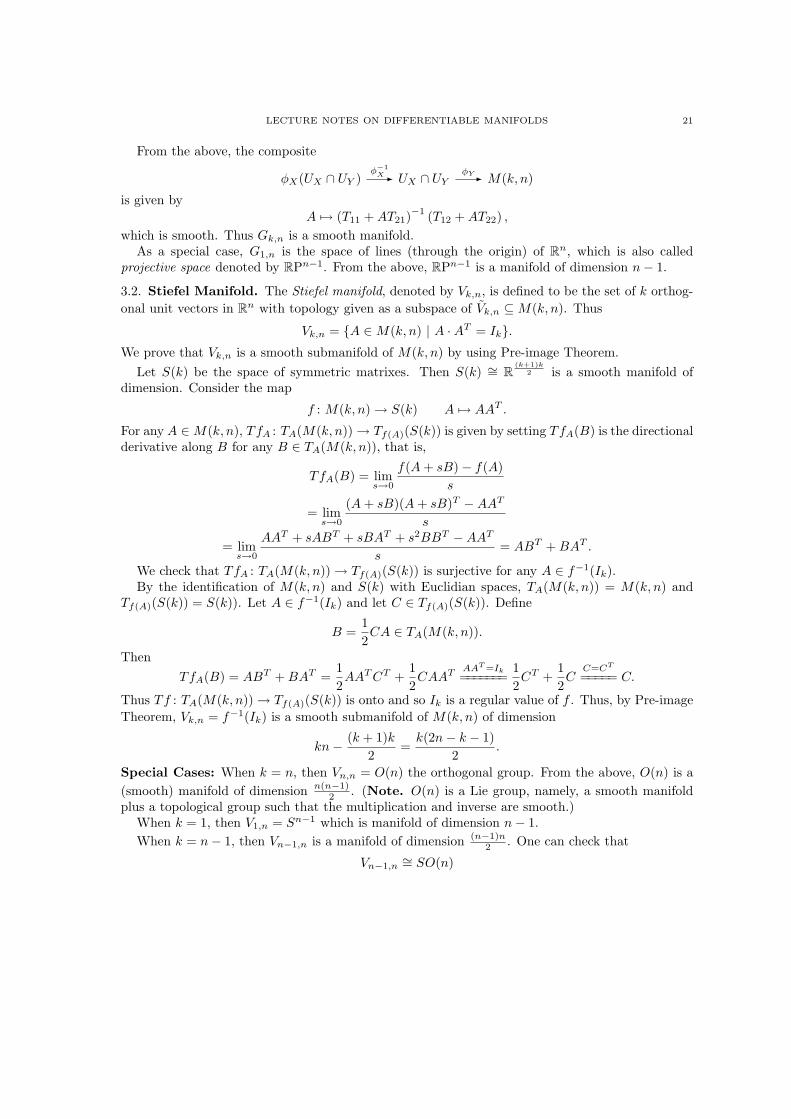
3.2. Stiefel Manifold. The Stiefel manifold, denoted by Vk,n, is defined to be the set of k orthog-onal unit vectors in Rn with topology given as a subspace of Vk,n ⊆M(k, n). Thus

Vk,n = A ∈M(k, n) | A ·AT = Ik.We prove that Vk,n is a smooth submanifold of M(k, n) by using Pre-image Theorem.

Let S(k) be the space of symmetric matrixes. Then S(k) ∼= R(k+1)k

2 is a smooth manifold ofdimension. Consider the map

f : M(k, n) → S(k) A 7→ AAT .

For any A ∈M(k, n), TfA : TA(M(k, n)) → Tf(A)(S(k)) is given by setting TfA(B) is the directionalderivative along B for any B ∈ TA(M(k, n)), that is,

TfA(B) = lims→0

f(A+ sB)− f(A)s

= lims→0

(A+ sB)(A+ sB)T −AAT

s

= lims→0

AAT + sABT + sBAT + s2BBT −AAT

s= ABT +BAT .

We check that TfA : TA(M(k, n)) → Tf(A)(S(k)) is surjective for any A ∈ f−1(Ik).By the identification of M(k, n) and S(k) with Euclidian spaces, TA(M(k, n)) = M(k, n) and

Tf(A)(S(k)) = S(k)). Let A ∈ f−1(Ik) and let C ∈ Tf(A)(S(k)). Define

B =12CA ∈ TA(M(k, n)).

ThenTfA(B) = ABT +BAT =

12AATCT +

12CAAT =======

AAT =Ik 12CT +

12C =====

C=CT

C.

Thus Tf : TA(M(k, n)) → Tf(A)(S(k)) is onto and so Ik is a regular value of f . Thus, by Pre-imageTheorem, Vk,n = f−1(Ik) is a smooth submanifold of M(k, n) of dimension

kn− (k + 1)k2

=k(2n− k − 1)

2.

Special Cases: When k = n, then Vn,n = O(n) the orthogonal group. From the above, O(n) is a(smooth) manifold of dimension n(n−1)

2 . (Note. O(n) is a Lie group, namely, a smooth manifoldplus a topological group such that the multiplication and inverse are smooth.)

When k = 1, then V1,n = Sn−1 which is manifold of dimension n− 1.When k = n− 1, then Vn−1,n is a manifold of dimension (n−1)n

2 . One can check that

Vn−1,n∼= SO(n)

22 JIE WU

the subgroup of O(n) with determinant 1. In general case, Vk,n = O(n)/O(n− k).As a space, Vk,n is compact. This follows from that Vk,n is a closed subspace of the k-fold

Cartesian product of Sn−1 because Vk,n is given by k unit vectors (~v1, . . . , ~vk)T in Rn that aresolutions to ~vi · ~vj = 0 for i 6= j, and the fact that any closed subspace of compact Hausdorff spaceis compact. The composite

Vk,n ⊂ - Vk,nπ-- Gk,n

is onto and so the Grassmann manifold Gk,n is also compact. Moreover the above composite is asmooth map because π is smooth and Vk,n is a submanifold. This gives the diagram

Vk,n ⊂submanifold- M(k, n)

submersion at IkA 7→ AAT

-- S(k)

Gk,n

smooth??

Note. By the construction, Gk,n is the quotient of Vk,n by the action of O(k). This gives identifi-cations:

Gk,n = Vk,n/O(k) = O(n)/(O(k)×O(n− k)).

4. Fibre Bundles and Vector Bundles

4.1. Fibre Bundles. A bundle means a triple (E, p,B), where p : E → B is a (continuous) map.The space B is called the base space, the space E is called the total space, and the map p is calledthe projection of the bundle. For each b ∈ B, p−1(b) is called the fibre of the bundle over b ∈ B.

Intuitively, a bundle can be thought as a union of fibres f−1(b) for b ∈ B parameterized by Band glued together by the topology of the space E. Usually a Greek letter ( ξ, η, ζ, λ, etc) is used todenote a bundle; then E(ξ) denotes the total space of ξ, and B(ξ) denotes the base space of ξ.

A morphism of bundles (φ, φ) : ξ → ξ′ is a pair of (continuous) maps φ : E(ξ) → E(ξ′) andφ : B(ξ) → B(ξ′) such that the diagram

E(ξ)φ- E(ξ′)

B(ξ)

p(ξ)

? φ- B(ξ′)

p(ξ′)

?

commutes.The trivial bundle is the projection of the Cartesian product:

p : B × F → B, (x, y) 7→ x.

Roughly speaking, a fibre bundle p : E → B is a “locally trivial” bundle with a “fixed fibre” F .More precisely, for any x ∈ B, there exists an open neighborhood U of x such that p−1(U) is a trivial


bundle, in other words, there is a homeomorphism φU : p−1(U) → U × F such that the diagram

U × Fφx- p−1(U)

U

π1

?========= U

p

?

commutes, that is, p(φ(x′, y)) = x′ for any x′ ∈ U and y ∈ F .Similar to manifolds, we can use “chart” to describe fibre bundles. A chart (U, φ) for a bundle

p : E → B is (1) an open set U of B and (2) a homeomorphism φ : U × F → p−1(U) such thatp(φ(x′, y)) = x′ for any x′ ∈ U and y ∈ F . An atlas is a collection of charts (Uα, φα) such thatUα is an open covering of B.

Proposition 4.1. A bundle p : E → B is a fibre bundle with fibre F if and only if it has an atlas.

Proof. Suppose that p : E → B is a fibre bundle. Then the collection (U(x), φx)|x ∈ B is an atlas.Conversely suppose that p : E → B has an atlas. For any x ∈ B there exists α such that x ∈ Uα

and so Uα is an open neighborhood of x with the property that p|p−1(U) : p−1(Uα) → Uα is a trivialbundle. Thus p : E → B is a fibre bundle.

Let ξ be a fibre bundle with fibre F and an atlas (Uα, φα). The composite

φ−1α φβ : (Uα ∩ Uβ)× F

φβ- p−1(Uα ∩ Uβ)φ−1

α- (Uα ∩ Uβ)× F

has the property thatφ−1α φβ(x, y) = (x, gαβ(x, y))

for any x ∈ Uα ∩ Uβ and y ∈ F . Consider the continuous map gαβ : Uαβ × F → F . Fixing any x,gαβ(x,−) : F → F , y 7→ gαβ(x, y) is a homeomorphism with inverse given by gβα(x,−). This givesa transition function

gαβ : Uα ∩ Uβ - Homeo(F, F ),where Homeo(F, F ) is the group of all homeomorphisms from F to F .

Exercise 4.1. Prove that the transition functions gαβ satisfy the following equation

(3) gαβ(x) gβγ(x) = gαγ(x) x ∈ Uα ∩ Uβ ∩ Uγ .

By choosing α = β = γ, gαα(x) gαα(x) = gαα(x) and so

(4) gαα(x) = x x ∈ Uα.

By choosing α = γ, gαβ(x) gβα(x) = gαα(x) = x and so

(5) gβα(x) = gαβ(x)−1 x ∈ Uα ∩ Uβ .We need to introduce a topology on Homeo(F, F ) such that the transition functions gαβ are

continuous. The topology on Homeo(F, F ) is given by compact-open topology briefly reviewed asfollows:

Let X and Y be topological spaces. Let Map(X,Y ) denote the set of all continuous maps fromX to Y . Given any compact set K of X and any open set U of Y , let

WK,U = f ∈ Map(X,Y ) | f(K) ⊆ U.

24 JIE WU

Then the compact-open topology is generated by WK,U , that is, an open set in Map(X,Y ) is anarbitrary union of a finite intersection of subsets with the form WK,U .

Map(F, F ) be the set of all continuous maps from F to F with compact open topology. ThenHomeo(F, F ) is a subset of Map(F, F ) with subspace topology.

Proposition 4.2. If Homeo(F, F ) has the compact-open topology, then the transition functionsgαβ : Uα ∩ Uβ → Homeo(F, F ) are continuous.

Proof. Given WK,U , we show that g−1αβ (WK,U ) is open in Uα ∩ Uβ . Let x0 ∈ Uα ∩ Uβ such that

gαβ(x0) ∈W(K,U). We need to show that there is a neighborhood V is x0 such that gαβ(V ) ⊆WK,U ,or gαβ(V × K) ⊆ U . Since U is open and gαβ : (Uα ∩ Uβ) × F → F is continuous, g−1(U) is anopen set of (Uα ∩Uβ)× F with x0 ×K ⊆ g−1

αβ (U). For each y ∈ K, there exist open neighborhoodsV (y) of x and N(y) of y such that V (x)×N(y) ⊆ g−1

αβ (U). Since N(y) | y ∈ K is an open cover

of the compact set K, there is a finite cover N(y1), . . . , N(yn) of K. Let V =n⋂j=1

V (yj). Then

V ×K ⊆ g−1αβ (U) and so gαβ(V ) ⊆WK,U .

Proposition 4.3. If F regular and locally compact, then the composition and evaluation maps

Homeo(F, F )×Homeo(F, F ) - Homeo(F, F ) (g, f) 7→ f gHomeo(F, F )× F - F (f, y) 7→ f(y)

are continuous.

Proof. Suppose that f g ∈ WK,U . Then f(g(K)) ⊆ U , or g(K) ⊆ f−1(U), and the latter is open.Since F is regular and locally compact, there is an open set V such that

g(K) ⊆ V ⊆ V ⊆ f−1(U)

and the closure V is compact. If g′ ∈ WK,V and f ′ ∈ WV ,U , then f ′ g′ ∈ WK,U . Thus WK,V andWV ,U are neighborhoods of g and f whose composition product lies in WK,U . This implies thatHomeo(F, F )×Homeo(F, F ) → Homeo(F, F ) is continuous.

Let U be an open set of F and let f0(y0) ∈ U or y0 ∈ f−10 (U). Since F is regular an locally

compact, there is a neighborhood V of y0 such that V is compact and y0 ∈ V ⊆ V ⊆ g−10 (U).

If g ∈ WV ,U and y ∈ V , then g(y) ∈ U and so the evaluation map Homeo(F, F ) × F → F iscontinuous.

Proposition 4.4. If F is compact Hausdorff, then the inverse map

Homeo(F, F ) - Homeo(F, F ) f 7→ f−1

is continuous.

Proof. Suppose that g−10 ∈WK,U . Then g−1

0 (K) ⊆ U or K ⊆ g0(U). It follows that

F rK ⊇ F r g0(U) = g0(F r U)

because g0 is a homeomorphism. Note that F rU is compact, F rK is open and g0 ∈WFrU,FrK .If g ∈WFrU,FrK , then, from the above arguments, g−1 ∈WK,U and hence the result.

Note. If F is regular and locally compact, then Homeo(F, F ) is a topological monoid, namelycompact-open topology only fails in the continuity of g−1. A modification on compact-open topologyeliminates this defect [1].


4.2. G-Spaces and Principal G-Bundles. Let G be a topological group and let X be a space.A right G-action on X means a(continuous) map µ : X ×G→ X, (x, g) 7→ x · g such that x · 1 = xand (x · g) ·h = x · (gh). In this case, we call X a (right) G-space. Let X and Y be (right) G-spaces.A continuous map f : X → Y is called a G-map if f(x · g) = f(x) · g for any x ∈ X and g ∈ G. LetX/G be the set of G-orbits xG, x ∈ X, with quotient topology.

Proposition 4.5. Let X be a G-space.1) For fixing any g ∈ G, the map x 7→ x · g is a homeomorphism.2) The projection π : X → X/G is an open map.

Proof. (1). The inverse is given by x 7→ x · g−1.(2) If U is an open set of X,

π−1(π(U)) =⋃g∈G

U · g

is open because it is a union of open sets, and so π(U) is open by quotient topology. Thus π is anopen map.

We are going to find some conditions such that π : X → X/G has canonical fibre bundle structurewith fibre G. Given any point x ∈ X/G, choose x ∈ X such that π(x) = x. Then

π−1(x) = x · g | g ∈ G = G/Hx,

where Hx = g ∈ G | x · g = x.For having constant fibre G, we need to assume that the G-action on X is free, namely

x · g = x =⇒ g = 1

for any x ∈ X. This is equivalent to the property that

x · g = x · h =⇒ g = h

for any x ∈ X. In this case we call X a free G-space.Since a fibre bundle is locally trivial (locally Cartesian product), there is always a local cross-

section from the base space to the total space. Our second condition is that the projection π : X →X/G has local cross-sections. More precisely, for any x ∈ X/G, there is an open neighborhood U(x)with a continuous map sx : U(x) → X such that π sx = idU(x).

(Note. For every point x, we can always choose a pre-image of π, the local cross-section meansthe pre-images can be chosen “continuously” in a neighborhood. This property depends on thetopology structure of X and X/G.)

Assume that X is a (right) free G-space with local cross-sections to π : X → X/G. Let x be anypoint in X/G. Let U(x) be a neighborhood of x with a (continuous) crosse-section sx : U(x) → X.Define

φx : U(x)×G - π−1(U(x)) (y, g) - sx(y) · gfor any y ∈ U(x).

Exercise 4.2. Let X be a (right) free G-space with local cross-sections to π : X → X/G. Then thecontinuous map φx : U(x)×G→ π−1(U(x)) is one-to-one and onto.

We need to find the third condition such that φx is a homeomorphism. Let

X∗ = (x, x · g) | x ∈ X, g ∈ G ⊆ X ×X.

26 JIE WU

A functionτ : X∗ - G

such thatx · τ(x, x′) = x′ for all (x, x′) ∈ X

is called a translation function. (Note. If X is a free G-space, then translation function is uniquebecause, for any (x, x′) ∈ X∗, there is a unique g ∈ G such that x′ = x · g, and so, by definition,τ(x, x′) = g.)

Proposition 4.6. Let X be a (right) free G-space with local cross-sections to π : X → X/G. Thenthe following statements are equivalent each other:

1) The translation function τ : X∗ → G is continuous.2) For any x ∈ X/G, the map φx : U(x)×G→ π−1(U(x)) is a homeomorphism.3) There is an atlas (Uα, φα of X/G such that the homeomorphisms

φα : Uα ×G - π−1(Uα)

satisfy the condition φα(y, gh) = φα(y, g) · h, that is φα is a homeomorphism of G-spaces.

Proof. (1) =⇒ (2). Consider the (continuous) map

θ : π−1(U(x)) - U(x)×G z 7→ (π(z), τ(sx(π(z)), z)).

Thenθ φx(y, g) = θ(sx(y) · g) = (y, τ(sx(y), sx(y) · g)) = (y, g),

φx θ(z) = φx(π(z), τ(sx(π(z)), z)) = sx(π(z)) · τ(sx(π(z)), z) = z.

Thus φx is a homeomorphism.(2) =⇒ (3) is obvious.(3) =⇒ (1). Note that the translation function is unique for free G-spaces. It suffices to show

that the restriction

τ(X) : X∗ ∩ (π−1(Uα)× π−1(Uα)) =(π−1(Uα)

)∗ - G

is continuous. Consider the commutative diagram

(Uα ×G)∗φ∗α∼=-(π−1(Uα)

)∗

G

τ(Uα ×G)

?=========== G.

τ(X)

?

Sinceτ(Uα ×G)((y, g), (y, h)) = g−1h

is continuous, the translation function restricted to(π−1(Uα)

)∗τ(X) = τ(Uα ×G) ((φα)∗)−1

is continuous for each α and so τ(X) is continuous.


Now we give the definition. A principal G-bundle is a free G-space X such that

π : X → X/G

has local cross-sections and one of the (equivalent) conditions in Proposition 4.6 holds.

Example. Let Γ be a topological group and let G be a closed subgroup. Then the action of Gon Γ given by (a, g) 7→ ag for a ∈ Γ and g ∈ G is free. Then translation function is given byτ(a, b) = a−1b, which is continuous. Thus Γ → Γ/G is principal G-bundle if and only if it has localcross-sections.

4.3. The Associated Principal G-Bundles of Fibre Bundles. We come back to look at fibrebundles ξ given by p : E → B with fibre F . Let (Uα, φα) be an atlas and let

gαβ : Uα ∩ Uβ - Homeo(F, F )

be the transition functions. A topological group G is called a group of the bundle ξ if1) There is a group homomorphism

θ : G - Homeo(F, F ).

2) There exists an atlas of ξ such that the transition functions gαβ lift to G via θ, that is,there is commutative diagram

Uα ∩ Uβgαβ- Homeo(F, F )

Uα ∩ Uβ

wwwwwwwwwgαβ - G,

θ

6

(where we use the same notation gαβ .)3) The transition functions

gαβ : Uα ∩ Uβ - G

are continuous.4) The G-action on F via θ is continuous, that is, the composite

G× Fθ×idF- Homeo(F, F )× F

evaluation- F

is continuous.We write ξ = (Uα, gαβ) for the set of transition functions to the atlas (Uα, φα).

Note. In Steenrod’s definition [13, p.7], θ is assume to be a monomorphism (equivalently, theG-action on F is effective, that is, if y · g = y for all y ∈ F , then g = 1.).

We are going to construct a principal G-bundle π : EG → B. Then prove that the total spaceE = F ×G EG and p : E → B can be obtained canonically from π : EG → B. In other words,all fibre bundles can obtained through principal G-bundles through this way. Also the topologicalgroup G plays an important role for fibre bundles. Namely, by choosing different topological groupsG, we may get different properties for the fibre bundle ξ. For instance, if we can choose G to betrivial (that is, gαβ lifts to the trivial group), then fibre bundle is trivial. We will see that the bundlegroup G for n-dimensional vector bundles can be chosen as the general linear group GLn(R). The

28 JIE WU

vector bundle is orientable if and only if the transition functions can left to the subgroup of GLn(R)consisting of n × n matrices whose determinant is positive. If n = 2m, then GLm(C) ⊆ GL2m(R).The vector bundle admits (almost) complex structure if and only if the transition functions can leftto GLm(C). (For manifolds, one can consider the structure on the tangent bundles. For instance,an oriented manifold means its tangent bundle is oriented.)

Proposition 4.7. If ξ is the set of transition functions for the space B and topological group G,then there is a principal G-bundle ξG given by

π : EG - B

and an atlas (Uα, φα) such that ξ is the set of transition functions to this atlas.

Proof. The proof is given by construction. Let

E =⋃α

Uα ×G× α,

that is E is the disjoint union of Uα ×G. Now define a relation on E by

(b, g, α) ∼ (b′, g′, β) ⇐⇒ b = b′, g = gαβ(b)g′.

This is an equivalence relation by Equations (3)-(5). Let EG = E/ ∼ with quotient topology andlet b, g, α for the class of (b, g, α) in EG. Define π : EG → B by

πb, g, α = b,

then π is clearly well-defined (and so continuous). The right G-action on EG is defined by

b, g, α · h = b, gh, α.

This is well-defined (and so continuous) because if (b′, g′, β) ∼ (b, g, α), then

(b′, g′h, β) = (b, (gαβ(b)g)h, β) = (b, gαβ(b)(gh), β) ∼ (b, gh, α).

Define φα : Uα ×G→ π−1(Uα) by setting

φα(b, g) = b, g, α,

then φα is continuous and satisfies π φα(b, g) = b and

φα(b, g) = b, 1 · g, α = b, 1, α · g

for b ∈ Uα and g ∈ G. The map φα is a homeomorphism because, for fixing α, the map∐β

(Uα ∩ Uβ)×G× β - Uα ×G (b, g′, β) 7→ (b, gαβ(b)g′)

induces a map π−1(Uα) → Uα ×G which the inverse of φα. Moreover,

φα(b, gαβ(b)g) = b, gαβ(b)g, α = b, g, β = θβ(b, g)

for b ∈ Uα ∩ Uβ and g ∈ G. Thus the (Uα, gαβ) is the set of transition function to the atlas(Uα, φα).


Let X be a right G-space and let Y be a left G-space. The product over G is defined by

X ×G Y = X × Y/(xg, y) ∼ (x, gy)

with quotient topology. Note that the composite

X × YπX - X

π - X/G

(x, y) 7→ x 7→ x

factors through X ×G Y . Let p : X ×G Y → X/G be the resulting map. For any x ∈ X/G, choosex ∈ π−1(x) ⊆ X, then

p−1(x) = π−1(x)×G Y = x× Y/Hx,

where Hx = g ∈ G | xg = x. Thus if X is a free right G-space, then the projection p : X ×G Y →X/G has the constant fibre Y .

Proposition 4.8. Let π : X → X/G be a (right) principal G-bundle and let Y be any left G-space.Then

p : X ×G Y - X/G

is a fibre bundle with fibre Y .

Proof. Consider a chart (Uα, φα) for π : X → X/G. Since the homeomorphism φα : Uα × G →π−1(Uα) is a G-map, there is a commutative diagram

Uα × Y === (Uα ×G)×G Yφα∼=- π−1(Uα)×G Y === p−1(Uα)

Uα

πUα

?=========== Uα

πUα

?============= Uα

p

?========== Uα

p

?

and hence the result.

Let ξ be a (right) principal G-bundle given by π : X → X/G. Let Y be any left G-space. Thenfibre bundle

p : X ×G Y - X/G

is called induced fibre bundle of ξ, denoted by ξ[Y ].Now let p : E → B is a fibre bundle with fibre F and bundle group G. Observe that the action

of Homeo(F, F ) on F is a left action because (f g)(x) = f(g(x)). Thus G acts by left on F viaθ : G→ Homeo(F, F ).

A bundle morphism

E(ξ)φ- E(ξ′)

B(ξ)

p(ξ)

? φ- B(ξ′)

p(ξ′)

?

30 JIE WU

is call an isomorphism if both φ and φ are homeomorphisms. (Note. this means that (φ−1, (φ)−1)are continuous.) In this case, we write ξ ∼= ξ′.

Theorem 4.9. Let ξ be a fibre bundle given by p : E → B with fibre F and bundle group G. Let ξG

be the principal G-bundle constructed in Proposition 4.7 according to a set of transitions functionsto ξ Then ξG[F ] ∼= ξ.

Proof. Let (Uα, φα) be an atlas for ξ. We write φα for φα in the proof of Proposition 4.7. Considerthe map θα given by the composite:

π−1(Uα)×G F φα × idF∼=

(Uα ×G× α)G × F === Uα × Fφα∼=- p−1(Uα).

From the commutative diagram

((Uα ∩ Uβ)×G× β)×G F(b, g′, y) 7→ (b, g′, gαβ(b)(y))

((b, g′, β), y) 7→ ((b, gαβ(b)g′, α), y)- ((Uα ∩ Uβ)×G× α)×G F

(Uα ∩ Uβ)× F

wwwwwwwww(b, y) 7→ (b, gαβ(b, y)) - (Uα ∩ Uβ)× F

wwwwwwwww

p−1(Uα ∩ Uβ)

∼= φβ

?

=========================================== p−1(Uα ∩ Uβ),

∼= φα

?

the map θα induces a bundle map

EG ×G Fθ - E(ξ)

B(ξ)?

====== B(ξ).?

This is an bundle isomorphism because θ is one-to-one and onto, and θ is a local homeomorphic byrestricting each chart. The assertion follows.

This theorem tells that any fibre bundle with a bundle group G is an induced fibre bundle ofa principal G-bundle. Thus, for classifying fibre bundles over a fixed base space B, it suffices toclassify the principal G-bundles over B. The latter is actually done by the homotopy classes fromB to the classifying space BG of G. (There are few assumptions on the topology on B such as B isparacompact.) The theory for classifying fibre bundles is also called (unstable) K-theory, which isone of important applications of homotopy theory to geometry. Rough introduction to this theoryis as follows:

There exists a universal G-bundle ωG as π : EG→ BG. Given any principal G-bundle ξ over B,there exists a (continuous) map f : B → BG such that ξ, as a principal G-bundle, is isomorphic to


the pull-back bundle f∗ωG given by

E(f∗ωG) = (x, y) ∈ B × EG | f(x) = π(y) - EG

B

(x, y) 7→ x

? f - BG.

π

?

Moreover, for continuous maps f, g : B → BG, f∗ωG ∼= g∗ωG if and only if f ' g, that is, there is acontinuous map (called homotopy) F : B× [0, 1] → BG such that F (x, 0) = f(x) and F (x, 1) = g(x).In other words, the set of homotopy classes [B,BG] is one-to-one correspondent to the set ofisomorphic classes of principal G-bundles over G.

Seminar Topic: The classification of principal G-bundles and fibre bundles. (References: forinstance [8, pp.48-58] Or [10, 11].)

4.4. Vector Bundles. Let F denote R, C or H-the real, complex or quaternion numbers. Ann-dimensional F-vector bundle is a fibre bundle ξ given by p : E → B with fibre Fn and an atlas(Uα, φα) in which each fibre p−1(b), b ∈ B, has the structure of vector space over F such thateach homeomorphism φα : Uα × Fn → p−1(Uα) has the property that

φα|b×Fn : b × Fn - p−1(b)

is a vector space isomorphism for each b ∈ Uα.Let ξ be a vector bundle. From the composite

(Uα ∩ Uβ)× Fn φβ- p−1(Uα ∩ Uβ)φ−1

α- (Uα ∩ Uβ)× Fn,

the transition functionsgαβ : Uα ∩ Uβ - Homeo(Fn,Fn)

have that property that, for each x ∈ Uαβ ,

gαβ(x) : Fn - Fn

is a linear isomorphism. It follows that the bundle group for a vector bundle can be chosen asthe general linear group GLn(F). By Theorem 4.9, we have the following.

Proposition 4.10. Let ξ be an n-dimensional F-vector space over B. Then there exists a principalGLn(F)-bundle ξGLn(F) over B such that ξ ∼= ξGLn(F)[Fn]. Conversely, for any principal GLn(F)-bundle over B, ξGLn(F)[Fn] is an n-dimensional F-vector bundle over B.

In other words, the total spaces of all vector bundles are just given by E(ξGLn(F))×GLn(F) Fn.

4.5. The Construction of Gauss Maps. The Grassmann manifold Gn,m(F) is the set of n-dimensional F-subspaces of Fm, that is, all n-F-planes through the origin, with the topology de-

scribed as in the topic on the examples of Manifolds. (If m = ∞, F∞ =∞⊕j=1

F.) Let

E(γmn ) = (V, x) ∈ Gn,m(F)× Fm | x ∈ V .

32 JIE WU

Exercise 4.3. Show thatp : E(γmn ) → Gn,m(F) (V, x) 7→ V

is an n-dimensional F-vector bundle, denoted by γmn . [Hint: By reading the topic on the examples ofmanifolds, check that Vn,m(F) → Gn,m(F) is a principal O(n,F), where O(n,R) = O(n), O(n,C) =U(n) and O(n,H) = Sp(n). Then check that E(γmn ) = Vn,m(F)×O(n,F) Fn.]

A Gauss map of an n-dimensional F-vector bundle in Fm (n ≤ m ≤ ∞) is a (continuous) mapg : E(ξ) → Fm such that g restricted to each fibre is a linear monomorphism.Example. The map

q : E(γmn ) → Fm (V, x) 7→ x

is a Gauss map.

Proposition 4.11. Let ξ be an n-dimensional F-vector bundle.1) If there is a vector bundle morphism

E(ξ)u- E(γmn )

B(ξ)

p(ξ)

? f- Gn,m(F)

p(γmn )

?

that is an isomorphism when restricted to any fibre of ξ, then q u : E(ξ) → Fm is a Gaussmap.

2) If there is a Gauss map g : E(ξ) → Fm, then there is a vector bundle morphism (u, f) : ξ →γmn such that qu = g.

Proof. (1) is obvious. (2). For each b ∈ B(ξ), g(p(ξ)−1(b)) is an n-dimensional F-subspace of Fmand so a point in Gn,m(F). Define the functions

f : B(ξ) → Gn,m(F) f(b) = g(p(ξ)−1(b)),

u : E(ξ) → E(γmn ) u(z) = (f(p(z)), g(z)).

The functions f and u are well-defined. For checking the continuity of f and u, one can look at alocal coordinate of ξ and so we may assume that ξ is a trivial bundle, namely, g : B(ξ)× Fn → Fmrestricted to each fibre is a linear monomorphism. Let e1, . . . , en be the standard F-bases for Fn.Then the map

h : B - Fm × · · · × Fm b 7→ (g(b, e1), g(b, e2), . . . , g(b, en))

is continuous. Since g restricted to each fibre is a monomorphism, the vectors

g(b, e1), g(b, e2), . . . , g(b, en)

are linearly independent and so

(g(b, e1), g(b, e2), . . . , g(b, en)) ∈ Vn,m(F)

for each b, where Vn,m(F) is the open Stiefel manifold over F. Thus

h : B - Vn,m(F) b 7→ (g(b, e1), g(b, e2), . . . , g(b, en))


is continuous and so the composite

f : Bh- Vn,m(F)

quotient-- Gn,m(F)

is continuous. The function u is continuous because the composite

E(ξ)u - E(γmn )

E(ξ)× E(ξ)

∆

? (f p(ξ))× g- Gn,m(F)× Fm?

∩

is continuous. This finishes the proof.

Let ξ be a vector bundle and let f : X → B(ξ) be a (continuous) map. Then the induced vectorf∗ξ is the pull-back

E(f∗ξ) = (x, y) ∈ X × E(ξ) |f(x) = p(y) - E(ξ)

X? f- B(ξ).

p

?

Proposition 4.12. There exists a Gauss map g : E(ξ) → Fm (n ≤ m ≤ ∞) if and only if

ξ ∼= f∗(γmn )

over B(ξ) for some map f : B(ξ) → Gn,m(F).

Proof. ⇐= is obvious.=⇒ Assume that ξ has a Gauss map g. From Part (2) of Proposition 4.11, there is a commutative

diagram

E(ξ)u- E(γmn )

B(ξ)

p(ξ)

? f- Gn,m(F).

p(γmn )

?

Since E(f∗γmn ) is defined to be the pull-back, there is commutative diagram

E(ξ)u- E(f∗γmn )

B(ξ)

p(ξ)

?====== B(ξ),

p

?

where u restricted to each fibre is a linear isomorphism because both vector-bundle has the samedimension and the Gauss map g restricted to each fibre is a monomorphism. It follows that

34 JIE WU

u : E(ξ) → E(f∗γmn ) is one-to-one and onto. Moreover u is a homeomorphism by considering alocal coordinate.

We are going to construct a Gauss map for each vector bundle over a paracompact space. First,we need some preliminary results for bundles over paracompact spaces. (For further information onparacompact spaces, one can see [3, 162-169].

A family of C = Cα | J of subsets of a space X is called locally finite if each x ∈ X admits aneighborhood Wx such that Wx ∩ Cα 6= ∅ for only finitely many indices α ∈ J . Let U = Uα andV = Vβ be two open covers of X. V is called a refinement of U if for each β, Vβ ⊆ Uα for some α.

A Hausdorff space X is called paracompact if it is regular and if every open cover of X admits alocally finite refinement.

Let U = Uα | α ∈ J be an open cover of a space X. A partition of unity, subordinate to U , isa collection λα | α ∈ J of continuous functions λα : X → [0, 1] such that

1) The supportsupp(λα) ⊆ Uα

for each α, where the support

supp(λα) = x ∈ X | λα(x) 6= 0is the closure of the subset of X on which λα 6= 0;

2) for each x ∈ X, there is a neighborhood Wx of x such that λλα|Wx

6≡ 0 for only finitelymany indices α ∈ J . (In other words, the supports of λα’s are locally finite.)

3) The equation ∑α∈J

λα(x) = 1

for all x ∈ X, where the summation is well-defined for each given x because there are onlyfinitely many non-zeros.

We give the following well-known theorem without proof. One may read a proof in [2, pp.17-20].

Theorem 4.13. If X is a paracompact space and U = Uα is an open cover of X, then thereexists a partition of unity subordinate to U .

Lemma 4.14. Let ξ be a fibre bundle over a paracompact space B. Then ξ admits an atlas withcountable charts.

Proof. Let (Uα, φα | α ∈ J be an atlas for ξ. We are going to find another atlas with countablecharts.

By Theorem 4.13, there is a partition of unity λα | α ∈ J subordinate to Uα | α ∈ J. Let

Vα = λ−1α (0, 1] = b ∈ B | λα(b) > 0.

Then, by the definition of partition of unity, Vα ⊆ Vα ⊆ Uα. For each b ∈ B, let

S(b) = α ∈ J | λα(b) > 0.Then, by the definition of partition of unity, S(b) is a finite subset of J .

Now for each finite subset S of J define

W (S) = b ∈ B |λα(b) > λβ(b) for each α ∈ S and β 6∈ S


=⋂

α ∈ Sβ 6∈ S

(λα − λβ)−1(0, 1].

Then W (S) is open because for each b ∈ W (S), by definition of partition of unity, there exists aneighborhood Wb of b such that there are finitely many supports intersect with Wb; and so the above(possibly infinite) intersection of open sets restricted to Wb is only a finite intersection of open sets.

Let S and S′ be two subsets of J such that S 6= S′ and |S| = |S′| = m > 0, where |S| is thenumber of elements in S. Then there exist α ∈ S r S′ and β ∈ S′ r S because S 6= S′ but S andS′ has the same number elements. We claim that

W (S) ∩W (S′) = ∅.

Otherwise there exists b ∈ W (S) ∩W (S′). By definition W (S), λα(b) > λβ(b) because α ∈ S andβ 6∈ S. On the other hand, λβ(b) > λα(b) because b ∈W (S′), β ∈ S′ and α 6∈ S′.

Now define

Wm =⋃

b ∈ B|S| = m

W (S(b))

for each m ≥ 1. We prove that (1) Wm | m = 1, . . . is an open cover of B; and (2) ξ restricted toWm is a trivial bundle for each m. (Then Wm induces an atlas for ξ.)

To check Wm is an open cover, note that each Wm is open. For each b ∈ B, S(b) is a finite setand b ∈ W (S(b)) because λβ(b) = 0 for β 6∈ S(b) and λα(b) > 0 for α ∈ S(b). Let m = |S(b)|, thenb ∈Wm and so Wm is an open cover of B.

Now check that ξ restricted to Wm is trivial. From the above, Wm is a disjoint union of W (S(b)).It suffices to check that ξ restricted to each W (S(b)) is trivial. Fixing α ∈ S(b), for any x ∈W (S(b)),then

λα(x) > λβ(x)

for any β 6∈ S. In particular, λα(x) > 0 for any x ∈ W (S(b)). It follows that W (S(b)) ⊆ Vα ⊆ Uα.Since ξ restricted to Uα is trivial, ξ restricted to W (S(b)) is trivial. This finishes the proof.

Note. From the proof, if for each b ∈ B there are at most k sets Uα with b ∈ Uα, then B admitsan atlas of finite (at most k) charts. [In this case, check that Wj = ∅ for j > k.]

Theorem 4.15. Any n-dimensional F-vector bundle ξ over a paracompact space B has a Gauss mapg : E(ξ) → F∞. Moreover, if ξ has an atlas of k charts, then ξ has a Gauss map g : E(ξ) → Fkn.

Proof. Let (Ui, φi)1≤i≤k be an atlas of ξ with countable or finite charts, where k is finite or infinite.Let λi be the partition of unity subordinate to Ui. For each i, define the map gi : E(ξ) → Fnas follows: gi restricted to p(ξ)−1(Ui) is given by

gi(z) = λi(z)(p2 φ−1i (z)),

where p2 φ−1i is the composite

p(ξ)−1(Ui)φ−1

i- Ui × Fn projection

p2- Fn;

36 JIE WU

and gi restricted to the outside of p(ξ)−1(Ui) is 0. Since the closure of λ−1i (0, 1] is contained in Ui,

gi is a well-defined (continuous) map. Now define

g : E(ξ) →k⊕i=1

Fn = Fkn g(z) =k∑i=1

gi(z).

This a well-defined (continuous) map because for each z, there is a neighborhood of z such thatthere are only finitely many gi are not identically zero on it.

Since each gi : E(ξ) → Fn is a monomorphism (actually isomorphism) on the fibres of E(ξ) overb with λi(b) > 0, and since the images of gi are in complementary subspaces of Fkn, the map g is aGauss map.

This gives the following classification theorem:

Corollary 4.16. Every vector bundle over a paracompact space B is isomorphic to an induced vectorbundle f∗(γ∞n ) for some map f : B → Gn,∞(F). Moreover every vector bundle over a paracompactspace B with an atlas of finite charts is isomorphic to an induced vector bundle f∗(γmn ) for some mand some map f : B → Gn,m(F).

Remarks: It can be proved that f∗γmn ∼= g∗γmn if and only if f ' g : B → Gn,m(F). From this,one get that the set of isomorphism classes of n-dimensional F-vector bundles over a paracompactspace B is isomorphic to the set of homotopy classes [B,Gn,∞(F)].

For instance, if n = 1 and F = R, G1,∞(R) ' BO(1) ' BZ/2 ' RP∞, where BG is so-calledthe classifying space of the (topological) group G, and [B,RP∞] = H1(B,Z/2), which states thatall line bundles are by the first cohomology with coefficients in Z/2Z. In particular, any real linebundles over a simply connected space is always trivial.

If n = 1 and F = C, then G1,∞(C) ' BU(1) ' BS1 ' CP∞, and [B,CP∞] = H2(B,Z), whichstates that all complex line bundles are by the second integral cohomology.

If n = 1 and F = H, then G1,∞(H) ' BSp(1) ' BS3 ' HP∞, and so [B,G1,∞(H)] = [B,HP∞].However, the determination of [B,HP∞] is very hard problem even when B are spheres. If B = Sn,then [B,HP∞] = πn−1(S3) that is only known for n less than 66 or so, by a lot of computationsthrough many papers. Some people even believe that it is impossible to compute the generalhomotopy groups πn(S3).

Seminar Topic: Gauss Maps and the Classification of Vector Bundles. (References: for instance [8,pp.26-29,31-33].)

A vector bundle is called of finite type if it has an atlas with finite charts. Given two vectorbundles ξ and η over B, the Whitney sum ξ ⊕ η is defined to be the pull-back:

E(ξ ⊕ η) - E(ξ)× E(η)

B? ∆

diagonal- B ×B.

p(ξ)× p(η)

?

Intuitively, ξ ⊕ η is just the fibrewise direct sum.


Proposition 4.17. For a vector bundle ξ over a paracompact space B, the following statement areequivalent:

1) The bundle ξ is of finite type.2) There exists a map f : B → Gn,m(F) such that ξ is isomorphic to f∗γmn .3) There exists a vector bundle η such that the Whitney sum ξ ⊕ η is trivial.

Proof. (1) =⇒ (2) follows from Corollary 4.16. (2) =⇒ (1) It is an exercise to check that γmn isof finite type by using the property that the Grassmann manifold Gn,m(F) = O(m,F)/O(n,F) ×O(m − n,F) is compact, where O(n,R) = O(n), O(n,C) = U(n) and O(n,H) = Sp(n). It followsthat ξ ∼= f∗γmn is of finite type.

(2) =⇒ (3). Let (γmn )∗ be the vector bundle given by

E((γmn )∗) = (V,~v) ∈ Gn,m(F)× Fm | ~v ⊥ V

with canonical projection E((γmn )∗) → Gn,m(F). Then γmn ⊕ (γmn )∗ is an m-dimensional trivialF-vector bundle. It follows that

f∗(γmn ⊕ (γmn )∗) = f∗(γmn )⊕ f∗((γmn )∗)

is trivial. Let η = f∗((γmn )∗). Then ξ ⊕ η is trivial.(3) =⇒ (2). The composite

E(ξ) ⊂ - E(ξ ⊕ η) = B × Fm - Fm

is a Gauss map into finite dimensional vector space, where m = dim(ξ ⊕ η). By Proposition 4.12,there is a map f : B → Gn,m such that ξ ∼= f∗γmn .

Corollary 4.18. Let ξ be a F-vector bundle over a compact (Hausdorff) space B. Then there is aF-vector bundle η such that ξ ⊕ η is trivial.

In the view of (stable) K-theory, the Whitney sum is an operation on vector bundles over a (fixed)base-space, where the trivial bundles (of different dimensions) are all regarded as 0. In this sense,the Whitney sum plays as an addition (that is associative and commutative with 0). The bundle ξwith property that ξ ⊕ η is trivial for some η means that ξ is invertible. Those who are interestedin algebra can push notions in algebra to vector bundles by doing constructions fibrewisely. Moregeneral situation possibly is the sheaf theory (by removing the locally trivial condition) that is prettyuseful in algebraic geometry. In algebraic topology, people also study the category whose objects arejust continuous maps f : E → B with fixed space B, or even more general category whose objectsare diagrams over spaces. In the terminology of fibre bundles, a map f : E → B is called a bundle(without assuming locally trivial).

5. Tangent Bundles and Vector Fields

5.1. Tangent Bundles. Let M be a differentiable manifold of dimension m. As a set, the tangentbundle

T (M) =⋃P∈M

TP (M),

the disjoint union of tangent spaces. We introduce topological and differential structure on T (M)in three stages:

38 JIE WU

(a) For an open subset V ⊆ Rm, T (V ) ∼= V ×Rm using the parallel translation isomorphisms ateach point. Take this differential structure on T (V ) by regarding V ×Rm as a subset of R2m.(That is, T (V ) is regarded as a differentiable manifold with only one chart T (V ) ∼= V ×Rm.)

(b) For a chart (U, φ) of M , there is a bijection

Tφ : T (U)∼=- T (φ(U)) ∼= φ(U)× Rm

which is a linear isomorphism on each tangent space Tφ : TP (M) - Tφ(P )(φ(U)), seeSubsection 2.4. Take the topological and differential structure on T (U) induced by Tφ.

(c) If (V, ψ) is another chart of M , from Diagram 1, there is a commutative diagram

TP (M)Tφ∼=- Tφ(P )(φ(U ∩ V ))

TP (M)

wwwwwwwwwTψ∼=- Tψ(P )(ψ(U ∩ V )),

T (ψ φ−1)

?

where T (ψ φ−1) is the linear isomorphism induced by the Jacobian matrix of the differ-entiable map ψ φ−1 : φ(U ∩ V ) → ψ(U ∩ V ). Thus there is a commutative diagram

(6)

T (U ∩ V )Tφ∼=- T (φ(U ∩ V ))

∼= - φ(U ∩ V )× Rm

T (U ∩ V )

wwwwwwwwwTψ∼=- T (ψ(U ∩ V ))

T (ψ φ−1)

? ∼= - ψ(U ∩ V )× Rm,

(P,~v) 7→ (ψ φ−1(P ), TP (ψ φ−1)(~v))

?

where TP (ψ φ−1) is the Jacobian matrix of the differentiable map ψ φ−1 : φ(U ∩ V ) →ψ(U ∩ V ) at the point P .

In other words, let (Uα, φα) be a differentiable, then the tangent bundle T (M) is a differentiablemanifold with a differentiable atlas given by

Tφα : T (Uα)∼=- T (φα(Uα)) ∼= φα(Uα)× Rm

and transition functions given as in Diagram 6. (Note. As a topological space, T (M) is the quotientspace of the disjoint union

∐αT (Uα) with equivalence relation given by Diagram 6.)

Proposition 5.1. The projection π : T (M) →M, ~vP 7→ P is a vector bundle over M . Moreover πis a differentiable submersion.

Example. The tangent bundle of spheres are given as follows:

T (Sn) = (x, y) ∈ Rn+1 × Rn+1 | |x| = 1, y ⊥ x.

The projection π : T (Sn) → Sn is given by (x, y) 7→ x.


Proposition 5.2. If f : Mm → Nn is differentiable, then Tf : TM → TN is also differentiablewith a morphism of vector bundles

TMTf - TN

M

π

? f - N.

π

?

Proof. By definition, f is differentiable means that there are atlases (Uα, φα) forM and (Vβ , φβ)for N such that the composites

Rm ⊇ φα(f−1(Vβ) ∩ Uα)φ−1

α

∼=- f−1(Vβ) ∩ Uα

f- Vβψβ

∼=- ψβ(Vβ) ⊆ Rn

are differentiable. There is a commutative diagram

φα(f−1(Vβ) ∩ Uα)× Rm ∼= T (φα(f−1(Vβ) ∩ Uα) Tφα T (f−1(Vβ) ∩ Uα) = Tf−1(T (Vβ)) ∩ T (Uα)

ψβ(Vβ)× Rn ∼= T (ψβ(Vβ))

Θ

?

TψβT (Vβ),

T f

?

whereΘ(P,~v) = (ψβ f φ−1

α (P ), D(ψβ f φ−1α ) |P (~v))

and D(ψβ f φ−1α ) |P is the Jacobian matrix of ψβ f φ−1

α at P . Thus Tf is differentiable. SinceTf restricted to each fibre is a linear transformation, (Tf, f) is a morphism of tangent bundles andhence the result.

5.2. Vector Fields. Let M be a differentiable manifold. A smooth cross-section X of the bundleprojection π : TM →M is called a vector field on M , that is, X : M → TM is a smooth map suchthat π X = idM .

Let f : M → R be a smooth function and let X,Y : M → TM be vector fields. Then the fibrewiseaddition

X + Y : M → TM b 7→ X(b) + Y (b)and scalar multiplication

f ·X : M → TM b 7→ f(b) ·X(b)are also vector fields on M .

Let C∞(M) denote the set of smooth functions onM . Then C∞(M) admits an algebraic structureover R given by

(f + g)(b) = f(b) + g(b) (fg)(b) = f(b)g(b).Let VF(M) denote the set of vector fields on M . Then VF(M) is an abelian group under X + Ywith

f(gX) = (fg)X f(X + Y ) = fX + fY (f + g)X = fX + gX

for f, g ∈ C∞(M) and X,Y ∈ VF(M). Thus we have the following.

Proposition 5.3. Let M be a smooth manifold. Then VF(M) is a module over C∞(M).

40 JIE WU

Let X be a vector field and let P be a point in M . Then X admits a local expression in thefollowing sense:

Let (U, φ) be a chart around P , that is φ : U∼=- φ(U) ⊆ Rm such that φ(P ) = 0. There is a

commutative diagram

UX|U- T (U)

Tφ- T (φ(U)) ∼= φ(U)× Rm

U

wwwwwwwwww========= U

π

? φ - φ(U).

proj.

?

Thus

(7) Tφ X|U (Q) =

(φ(Q),

m∑i=1

ξiU (Q)∂

∂xi

∣∣∣∣Q

)for Q ∈ U . If (V, ψ) is another chart around P with ψ(P ) = 0, then the change of coordinates isobtained from the diagram

ψ(U ∩ V )× Rm ∼= T (ψ(U ∩ V )) Tψ T (U ∩ V )Tφ- T (φ(U ∩ V )) ∼= φ(U ∩ V )× Rm

ψ(U ∩ V )?

ψU ∩ V

π

? φ - φ(U ∩ V ).

proj.

?

Now we are going to describe an action of VF(M) on C∞(M). Let X be a vector field and letf be a smooth function on M . Then Xf is a smooth function on M defined as follows:

Given any P ∈M , let (U, φ) be a chart around P such that φ(P ) = 0,

(8) (Xf)(P ) =m∑i=1

ξiU (P )∂(f φ−1)

∂xi(0).

The picture is as follows:

UX|U- TU

Tφ- T (φ(U)) ∼= φ(U)× Rm(x,~v) 7→ D~v(fU φ−1)(x)- R

U

π

? φ - φ(U)? f |U φ−1

- R.

Exercise 5.1. Let X be a vector field on M and let f : M → R be a smooth function. Prove thatXf is well-defined smooth function on M . [Hint: Since smooth is local property, it suffices to checkthat Xf is well-defined, that is, to check that if (V, ψ) is another chart around P such ψ(P ) = 0


and ψ φ−1 smooth on φ(U ∩ V ), thenm∑i=1

ξiU (P )∂(f φ−1)

∂xi(0) =

m∑i=1

ξiV (P )∂(f ψ−1)

∂yi(0)

by using chain rule. Note. From the proof, we need the condition that ψ φ−1 is differentiable. Sothe definition of Xf depends on the differential structure of M .]

The proof of the following proposition follows from the definition.

Proposition 5.4. The action of VF(M) on C∞(M) satisfies the following rules:

X(f + g) = Xf +Xg X(fg) = Xf · g + f ·Xgfor X ∈ VF(M) and f, g ∈ C∞(M). In other words, for each X ∈ VF(M), the operation

DX : C∞(M) - C∞(M) f 7→ Xf

is a derivation on the algebra C∞(M).

Let Der(C∞(M)) denote the set of derivations on C∞(M). Then Der(C∞(M)) is a module overC∞(M) under the operations: for D1, D2 ∈ Der(C∞(M)) and g ∈ C∞(M), the derivations D1 +D2

and gD1 are given by

(D1 +D2)(f) = D1(f) +D2(f) (gD1)(f) = g ·D1(f).

Theorem 5.5. The function

Φ: VF(M) - Der(C∞(M)) X 7→ DX

is an isomorphism of C∞(M)-modules.

We need a lemma for proving Theorem 5.5.

Lemma 5.6. Let h be a smooth function defined on a neighborhood U of P on M . There is a(small) neighborhood V of P such that V ⊆ U , and a smooth function g on M such that g = h onV and g = 0 on the complement M r U of U

Sketch. First choose a small open neighborhood W of P such that W ⊆ U . For W , check that thereare small ε1- and ε2-neighborhoods Vε1 ⊆ Vε2 ⊆W of P with ε2 > ε1, and a smooth function f with0 ≤ f ≤ 1, f = 1 on Vε1 and f = 0 on M r Vε2 .

Next define

g(Q) =f(Q)h(Q) for Q ∈ U

0 for Q ∈M \ U.

Proof of Theorem 5.5. Since

ΦX+Y = ΦX + ΦY ΦgX = gΦX ,

the function Φ is a morphism of C∞(M)-modules.Step 1. Ker(Φ) = 0.

Let X be a vector field on M such that DX = 0, that is Xf = 0 for all f ∈ C∞(M). For eachP ∈M , let (U, φ) be a chart around P with φ(P ) = 0, from Equation 8

(Xf)(P ) =m∑i=1

ξiU (P )∂(f φ−1)

∂xi(0) = 0 for any f ∈ C∞(M).

42 JIE WU

Let hj be smooth function defined on a small neighborhood of P such that hj φ−1 = xj on asmall neighborhood of 0. By Lemma 5.6, there exists fj ∈ C∞(M) such that fj = hj in a smallneighborhood of P . By inputting fj into the above equation,

0 = (Xfj)(P ) =m∑i=1

ξiU (P )∂(fj φ−1)

∂xi(0) =

m∑i=1

ξiU (P )∂xj

∂xi(0) = ξj(U)(P ).

for j = 1, . . . ,m. Thus

X(P ) =m∑i=1

ξiU (P )∂

∂xi= 0

for any given P ∈M and so X = 0, that is Ker(Φ) = 0.

Now we are going to show that Φ is onto, that is, given any derivation D on C∞(M), we constructa vector field X such that DX = D, by two steps.

Step 2. If f is a smooth function on M such that f = 0 at all points of an open set U of M , thenDf = 0 on U .

Let P be any point in U . By Lemma 5.6, there are neighborhoods UP and WP of P , and asmooth function fP ∈ C∞(M) such that

WP ⊆ UP ⊆ U, fP |WP= 1 fP |MrUP

= 0.

Set g = 1 − fP . Then gf = f because, if Q ∈ UP , then f(Q) = 0 and g(Q)f(Q) = f(Q) = 0 forQ ∈ UP , and if Q 6∈ UP , then g(Q) = 1− fP (Q) = 1, and so g(Q)f(Q) = f(Q) for Q 6∈ UP .

Now since D is a derivation, Df = D(gf) = (Dg)f + g(Df) and so, for any given P ∈ U ,

(Df)(P ) = (Dg(P ))f(P ) + g(P )(Df(P )) = (Dg(P )) · 0 + 0 · (Df(P )) = 0

because f(P ) = 0 and g(P ) = 1− fP (P ) = 1− 1 = 0 as P ∈WP ⊆ U .Step 3. Construct the vector field X : M → TM such that Xf = D(f) for any f ∈ C∞(M).

Let P be an arbitrary point in M , and let h be any smooth function defined on a neighborhoodV of P . By Lemma 5.6, there a neighborhood U (U ⊆ V ) and an f ∈ C∞(M) such that f = hon U . If f ′ ∈ C∞(M) is also equal to h on U , then, by Step 2, Df = Df ′ on U . Hence, for anyf ∈ C∞(M) agreeing h on a neighborhood of P , the value of Df at P is independent on the choiceof f .

Now let (U, φ) be a chart around P . By Proposition 1.3, there exist real numbers a1, a2, . . . , an ∈R such that

(9) D(h)(P ) =n∑i=1

ai∂(h φ−1)

∂xi(P )

for any h ∈ C∞(U), where ai depends on D and P but is independent on h. Define a functionX : M → TM, P 7→ X(P ), such that

Tφ X(P ) =m∑i=1

ai∂

∂xi.

Then, for any f ∈ C∞(M), (Xf)(P ) = (Df)(P ) for any given P and so Xf = Df .


To show that X is smooth, it suffices to show that X is smooth in a small neighborhood of P .Let hj ∈ C∞(U) such that hj φ−1 = xj . By lemma 5.6, there exists a small neighborhood Vj(Vj ⊆ U) of P and fj ∈ C∞(M) such that fj = hj on Vj . From Equation 9,

D(fj)(Q) =m∑i=1

ai(Q)∂xj

∂xi(Q) = aj(Q)

for Q ∈ Vj . Thus aj is smooth on Vj and so X is smooth onm⋂j=1

Vj . This finishes the proof.

One of the important consequences of Theorem 5.5 is to discover the Lie algebra structure onvector fields, namely, given vector fields X and Y , we can construct canonical new vector field [X,Y ]called commutator product or bracket of X and Y .

Let’s first look at the structure on Der(C∞(M)). Let D1 and D2 be two derivations on C∞(M).The commutator product [D1, D2] : C∞(M) → C∞(M) is linear map defined by

[D1, D2](f) = D1(D2(f))−D2(D1(f)).

Lemma 5.7. Let D1, D2 be derivations on C∞(M). Then [D1, D2] is also a derivation on M .Moreover the following identities hold:

(10) [D1, D2] = −[D2, D1] [D1, [D2, D3]] + [D2, [D3, D1]] + [D3, [D1, D2]] = 0.

The latter is called Jacobi identity

Proof.[D1, D2](fg) = D1(D2(fg))−D2(D1(fg))

= D1(D2(f)g + fD2(g))−D2(D1(f)g + gD1(f))

= D1(D2(f))g +D2(f)D1(g) +D1(f)D2(g) + fD1(D2(g))

−D2(D1(f))g −D1(f)D2(g)−D2(f)D1(g)− fD2(D1(g))

= ([D1, D2](f))g + f([D1, D2](g)).Check the Jacobi identity by yourself.

Now given vector fields X and Y , then DX and DY are derivations on C∞(M). By Theorem 5.5,there is a unique vector field [X,Y ] such that

D[X,Y ] = [DX , DY ]

because [DX , DY ] is also a derivation. In other words,

[X,Y ]f = X(Y f)− Y (Xf)

for all f ∈ C∞(M). (Note. The composition f 7→ X(Y f) does not define a vector field in generalbecause it is not a derivation.)

Exercise 5.2. Prove the following identities for the bracket of vector fields:(1). [X + Y,Z] = [X,Z] + [Y, Z];(2). [X,Y + Z] = [X,Y ] + [X,Z];(3). [X,Y ] = −[Y,X];(4). [fX, gY ] = fg[X,Y ] + f(Xg)Y − g(Y f)X, for f, g ∈ C∞(M);(5). [X, [Y,Z]] + [Y, [Z,X]] + [Z, [X,Y ]] = 0.

44 JIE WU

Let F be any field. A vector space V (possibly infinitely dimensional) is called a Lie algebra overF if there is a bi-linear operation: [X,Y ] for X,Y ∈ V such that

[X,Y ] = −[Y,X] [X, [Y, Z]] + [Y, [Z,X]] + [Z, [X,Y ]] = 0

for all X,Y, Z ∈ V .

Theorem 5.8. Let M be a smooth manifold. Then VF(M) is a Lie algebra over R and Φ: VF(M) →Der(C∞(M)) is an isomorphism of Lie algebras.

5.3. Vector Fields on Spheres. In this subsection, we consider the very classical problem ofdetermining when a sphere Sn has a single unit vector field on it. A unit vector field means a vectorfield X : Sn → TSn such that |X(P )| = 1 for each P . Note that

TSn = (P,~v) ∈ Rn+1 ⊕ Rn+1 | |P | = 1, P · ~v = 0.Thus a vector field X : Sn → TSn can be written as a map

P 7→ (P, φX(P )),

where φX : Sn → Rn+1 is a smooth map such that P · φX(P ) = 0. Conversely, any smooth mapφ : Sn → Rn+1 such that P · φ(P ) = 0 defines a vector field X. If X is a unit vector field, then thesmooth map φX : Sn → Rn+1 satisfies two equations:

|φ(P )| = 1 P · φ(P ) = 0

for all P ∈ Sn. The first equation tells that φX is a smooth map from Sn → Sn.

Proposition 5.9. If Sn−1 has k orthogonal unit vector fields X1, . . . , Xk, then Snq−1 has k orthog-onal unit vector fields X1, . . . , Xk.

Proof. By the assumption there are maps φi : Sn−1 → Rn such that

P · φi(P ) = 0 φi(P ) · φj(P ) = δij

for all P ∈ Sn−1 and 1 ≤ i, j ≤ k. Consider Snq−1 as the join of q-copies of Sn−1, that is,

Snq−1 =

(t1P1, t2P2, . . . , tqPq) ∈ (Rn)⊕q = Rnq | Pi ∈ Sn−1, 0 ≤ ti ≤ 1,

q∑i=1

t2i = 1

.

Define φi : Snq−1 → Rnq by

φi(t1P1, t2P2, . . . , tqPq) = (t1φi(P1), t2φi(P2), . . . , tqφi(Pq)).

Then P · φi(P ) = 0 and φi(P ) · φj(P ) = δij for all P ∈ Snq−1. This defines k-orthogonal unit vectorfields on Snq−1.

Corollary 5.10. Every odd sphere S2q−1 has a unit vector field on it.

Proof. It suffices to show that S1 has a unit vector field, which is just given by φ : S1 → S2, (x1, x2) 7→(−x2, x1).

Proposition 5.11. If Sn has a unit vector field, then there is a deformation H : Sn × [0, 1] → Sn

such thatH(P, 0) = P H(P, 1) = −P

for all P ∈ Sn.


Proof. By the assumption, there is a map φ : Sn → Rn+1 such that P ·φ(P ) = 0 and |φ(P )| = 1 forall P ∈ Sn. Define H : Sn × [0, 1] → Sn by

H(P, t) = cos(πt)P + sin(πt)φ(P ).

Then H(P, 0) = P and H(P, 1) = −P for all P ∈ Sn. [Note. This deformation is on the greatcircle from P to −P in the direction φ(P ).]

The proof of the following theorem uses a result from algebraic topology that the antipodal mapa : Sn → Sn, x 7→ −x is homotopic to the identity map if and only if n is odd.

Theorem 5.12. The sphere Sn admits a unit vector field on it if and only if n is odd. Thus anyeven sphere has no unit vector fields.

Proof of the case n = 2 by assuming fundamental groups. We only prove that S2 has no unit vectorfields. Let SO(n) be the subgroup of O(n) consisting of orthogonal matrices of determinant +1.There is a principal G-bundle:

SO(2)j- SO(3)

π- S2,

which can be obtained by considering

S2 = (1, 0, 0) ·A | A ∈ SO(3)

the orbit space.Suppose that S2 has a (continuous) unit vector field. Then there is a (continuous) map φ : S2 →

R3 such that x · φ(x) = 0 and |φ(x)| = 1 for all x ∈ S2. Define a map s : S2 → SO(3) by

s(x) =

xφ(x)

x× φ(x)

.

Then s is a cross-section to the bundle projection π : SO(3) → S2, that is π s = idS2 . Define

θ : S2 × SO(2) - SO(3) (x, g) 7→ s(x) · g.

Then θ is continuous, one-to-one and onto and so θ is a homeomorphism because these are compactspaces. By applying the fundamental groups,

θ∗ : π1(S2 × SO(2)) = π1(S2)× π1(SO(2))∼=- π1(SO(3)).

By using the facts that π1(S2) = 0, SO(2) = S1, π1(S1) = Z, π1(SO(3)) = Z/2, θ∗ : Z ∼= Z/2 andhence a contradiction.

6. Riemann Metric and Cotangent Bundles

6.1. Riemann and Hermitian Metrics on Vector Bundles. If x ∈ R, let x = x, and ifz = x+ iy ∈ C, let z = x− iy. Let F denote either R or C.

Let V be a vector space over F. An inner product on V is a function β : V × V → F, the field ofscalars, such that

1) β(ax+a′x′, y) = aβ(x, y)+a′β(x′, y), β(x, by+b′y′) = bβ(x, y)+b′β(x, y′) for x, x′, y, y′ ∈ Vand a, a′, b, b′ ∈ F.

2) β(x, y) = β(y, x) for x, y ∈ V .3) β(x, x) ≥ 0 in R and β(x, x) = 0 if and only if x = 0.

46 JIE WU

With an inner product β on V we can define what it means for x and y to be perpendicular, thatis, β(x, y) = 0. On Rn and Cn there is a natural inner product, the Euclidean inner product, given

by β(x, y) = x · y =n∑i=1

xiyi. These formulas hold for R∞ and C∞.

Definition 6.1. Let ξ be a real or complex vector bundle over B. A Riemannian or Hermitianmatric on ξ is a function β : E(ξ ⊕ ξ) → F such that, for each b ∈ B, β restricted to the fibrep−1(b) × p−1(b) is an inner product on p−1(b). The Riemannian metric refers to F = R and theHermitian metric to F = C.

For instance, Let εk be the k-dimensional trivial bundle over B. Then β(b, x, x′) = x · x′ is aRiemannian metric in the real case and Hermitian metric in the complex case.

Theorem 6.2. Every real or complex vector bundle with a Gauss map has a Riemannian or Her-mitian metric.

Proof. Let g : E(ξ) → F∞ be a Gauss map. Define β : E(ξ ⊕ ξ) → F by the relation

β(b, x, x′) = g(b, x) · g(b, x′)for x, x′ ∈ p−1(b). Since g is continuous and a linear monomorphism on each fibre, β is a Riemannianmetric or Hermitian metric.

Corollary 6.3. Every vector bundle over a paracompact space has a metric.

Theorem 6.4. Let0 - ξ

u- ηv- ζ - 0

be a short exact sequence of vector bundles over B, that is, restricted to each fibre, u is a linearmonomorphism, Im(u) = Ker(v), v is a linear epimorphism, and u, v are identity on the base-spaceB. Let β be a metric on η. Then there is a morphism of vector bundles w : ξ ⊕ ζ - η splittingthe above exact sequence in the sense of the following commutative diagram

0 - ξu - η

v - ζ - 0

0 - ξ

wwwwwwwwww⊂

i - ξ ⊕ ζ

w

6

j -- ζ

wwwwwwwwww- 0,

where i is the inclusion of the first factor, and j is the projection onto the second factor.

Proof. Let ξ′ denote Imu, where E(ξ′) ⊆ E(η. Let E(ζ ′) be the subset of x′ ∈ E(η) such thatβ(x, x′) = 0 for all x ∈ E(ξ′) with pη(x) = pη(x′). (That is, ζ ′ is the fibrewise orthogonal complementof ξ′.)

The compositev|ζ′ : ζ ′ ⊆ η

v- ζ

is a bundle isomorphism over B because it is an linear isomorphism on each fibre and identity onthe base-space.

Define w to be the composite

w : ξ ⊕ ζu⊕(v|ζ′ )

−1

- ξ′ ⊕ ζ ′fibrewise addition- η.


Then w is a bundle isomorphism because it is a linear isomorphism on each fibre and identity onthe base-space.

The commutativity of the diagram follows from the construction of w. This proves the theorem.

Corollary 6.5. Let

E(ξ)u - E(η)

B?

========= B?

be a morphism of vector bundles.(1). If u is a linear epimorphism on each fibre and ξ has a metric, then

ξ ∼= η ⊕ ξ′

for some vector bundle ξ′ over B.(2). If u is a linear monomorphism on each fibre and η has a metric, then

η ∼= ξ ⊕ ζ

for some vector bundle ζ over B.

Example 6.6. Let f : M → N be a smooth immersion. Then there is morphism of vector bundles

Tf : TM → TN

which is a linear monomorphism on each fibre. Consider the commutative diagram

TM ⊂u- f∗TN

v - TN

pull back

M?

======== M? f - N,

?

where u is a linear monomorphism on each fibre and v : E(f∗T (N))b - Tf(b)N is an isomorphism.If M is paracompact, then every vector bundle over M has a metric and so the vector bundle f∗TNhas an orthogonal decomposition

f∗TN ∼= TM ⊕ νM.

The vector bundle νM → M is called the normal bundle of M with respect to the immersion f .(For smooth curves in R2 or R3, one can check that νM consists of normal vectors.) If M is asubmanifold of N , the normal bundle can be used for constructing so-called tubular neighborhoodof M .

Seminar Topic. The exponential map and tubular neighborhoods. [Reference: Serge Lang, dif-ferential manifolds, pp.95-98.]

48 JIE WU

6.2. Constructing New Bundles Out of Old and Cotangent Bundle. Let F be R, C or H.Let V be the category of all finite dimensional F-vector spaces and all linear isomorphisms. Let

T : V × V × · · · V - V

be a functor in k variables, that is,

1) to each sequence (V1, . . . , Vk) of vector spaces T (V1, . . . , Vk) ∈ V and2) to each fi : Vi →Wi for 1 ≤ i ≤ k of linear isomorphisms an isomorphism

T (f1, . . . , fk) : T (V1, . . . , Vk) - T (W1, . . . ,Wk)

so that3) T (idV1 , . . . , idVk

) = idT (V1,...,Vk) and4) T (f1 g1, . . . , fk gk) = T (f1, . . . , fk) T (g1, . . . , gk).

A functor T : V × · · · × V → V is called continuous if T (f1, . . . , fk) depends continuously onf1, . . . , fk.

Let T : V×· · ·×V → V be a continuous functor of k variables, and let ξ1, . . . , ξk be vector bundlesover a common base-space B. Then a new bundle over B is constructed as follows. For each b ∈ Blet

Fb = T (Fb(ξ1), . . . , Fb(ξk)).

Let E denote the disjoint union of Fb and define p : E → B by p(Fb) = b.

Theorem 6.7. There exists a canonical topology for E so that p : E → B is a F-vector bundle overB with fibre Fb.

The bundle is denoted by T (ξ1, . . . , ξk).

Proof. Let ξi be ni-dimensional F-vector bundle over B. There is a principle GLni(F)-bundle

ξGLni

(F)

i given by πi : Ei → B such that ξi = ξGLni

(F)

i [Fni ] is given by

Ei ×GLni(F) Fni - B.

Let m = dimF T (Fn1 , . . . ,Fnk). Since T is continuous functor, the function

T : GLn1(F)× · · · ×GLnk(F) - GLm(F) (f1, . . . , fk) 7→ T (f1, . . . , fk)

is continuous group homomorphism.Let the group GLn1(F)× · · · ×GLnk

(F) act on Fm via T , that is, the action is given by

(f1, . . . , fk) · x := T (f1, . . . , fk)(x)

for x ∈ Fm and f1, . . . , fk ∈ GLni(F). Then the vector bundle p : E → B is given by the pull-back

E - (E1 × · · · × Ek)×GLn1 (F)×···×GLnk(F) Fm

B

p

? ∆ - B × · · · ×B

π1 × · · · × πk

?

and hence the result.


Remark 1. There is a different proof by looking at local coordinate system. Our proof here is touse the fact that any vector bundle is the induced from a principal G-bundle. Similar results worksfor general fibre bundles.

Remark 2. From the proof, the new bundle T (ξ1, . . . , ξk) is obtained from a new bundle over theself Cartesian product of B via the diagonal map.

Proposition 6.8. Let ξ be a vector bundle over B. Then there is a canonical dual bundle ξ∗ overB such that each fibre is the dual vector space of the corresponding fibre of ξ.

Proof. The left action of the general linear group on Fn induces a canonical right action on the dualspace of Fn and then switch it to the left action.

Let gαβ be the transitive functions of ξ, that is, gαβ is obtained from

(Uα ∩ Uβ)× Fn φβ- p−1(Uαβ)φ−1

α- (Uα ∩ Uβ)× Fn (b, x) 7→ (b, gαβ(b, x)).

Then the transitive functions for ξ∗ are given by(g−1αβ

)∗.

In differential geometry, it is important to construct new bundles out of old. For differentiablemanifolds, we can start with the tangent bundles and then construct various new bundles from thetangent bundles. Below we list some examples:

1. The Whitney sum ξ ⊕ η is induced from the functor T : V × V → V, (V,W ) 7→ V ⊕W .

2. The dual bundle ξ∗ is induced from the (contravariant) functor T (V ) = V ∗ = Hom(V,F).

3. The vector space Hom(V,W ) of linear transformations gives a functor T : Vop×V → V, where Vop

is the opposite category of V by changing the linear isomorphism f to be f−1. [Note. Hom(V,W )is contravariant on V .]

4. T is obtained by the vector space of all symmetric bi-linear transformations from V × V to W .

5. The tensor product V ⊗W . [We will go through tensor products.]

6. The k-th symmetric product of V . [We will go through symmetric products.]

7. The k-th exterior product of V . [We will go through exterior products.]

8. The vector space of all 4-linear transformations K : V × V × V × V × V → R satisfying thesymmetry relations:

K(v1, v2, v3, v4) = K(v3, v4, v1, v2) = −K(v1, v2, v4, v3),

K(v1, v2, v3, v4) +K(v1, v4, v2, v3) +K(v1, v3, v4, v2) = 0.

[This last example is from the theory of Riemann curvature.]

50 JIE WU

6.3. Cotangent Bundles and Co-vector Fields. Let M be a differentiable manifold. The cotan-gent bundle T ∗M is defined to be the dual bundle of the tangent bundle of M .

Proposition 6.9. If a vector bundle ξ has metric, then ξ is isomorphic to its dual bundle ξ∗.

Proof. Let 〈−,−〉 : V ×V → F be any inner product on V . There is a canonical linear isomorphismθ : V → V ∗ defined by

θ(y)(x) = 〈x, y〉.We just need to show that θ induces a bundle isomorphism. Let gαβ be transitive functions forξ. From the commutative diagram

(Uα ∩ Uβ)× Fn × Fnφβ- p−1

ξ (Uα ∩ Uβ)(b, x, x′) 7→ (b, β(x, x′))- (Uα ∩ Uβ)× F

(Uα ∩ Uβ)× Fn × Fn

id×gαβ(b,−)× gαβ(b,−)

? φα- p−1ξ (Uα ∩ Uβ)

wwwwwwwww(b, x, x′) 7→ (b, β(x, x′))- (Uα ∩ Uβ)× F,

wwwwwwwwwthe transitive functions gαβ preserves the inner products, that is,

〈gαβ(b, x), gαβ(b, y)〉 = 〈x, y〉.

By using this, we check that the following diagram

(Uα ∩ Uβ)× Fnθ- (Uα ∩ Uβ)×Hom(Fn,F)

(Uα ∩ Uβ)× Fn

id×gαβ(b,−)

? θ- (Uα ∩ Uβ)×Hom(Fn,F)

id×(gαβ(b,−)−1

)∗?

commutes.Let p2 : (Uα ∩ Uβ)× Hom(Fn,F) → Hom(Fn,F) be the projection to the second coordinate. For

any (b, x) ∈ (Uα ∩ Uβ)× Fn and y ∈ Fn, then

p2 θ (id×gαβ(b, x)(y) = 〈y, gαβ(b, x)〉

= 〈gαβ(b, z), gαβ(b, x)〉 = 〈z, x〉,where z = gαβ(b,−)−1(y), and

p2 (id××

(gαβ(b,−)−1

)∗) θ(b, x)(y) = 〈gαβ(b,−)−1(y), x〉 = 〈z, x〉.

Thus the above diagram commutes and hence θ induces a bundle isomorphism.

Corollary 6.10. Let M be a paracompact differentiable manifold. Then the cotangent bundle T ∗Mis isomorphic to the tangent bundle TM .

Note. The geometric means of tangent bundle and cotangent bundle are different. The localcoordinate system for tangent bundle is given by ∂

∂xi, while the local coordinate system for the

cotangent bundle is dxi, where dxi is the differential of the function (x1, . . . , xn) → xi which isthe dual of ∂i = ∂

∂xi.


Let M be a differentiable manifold. A (smooth) cross-section of the cotangent bundle p : T ∗M →M is called a covector field or 1-form. In other words, a 1-form is a smooth map ω : M → T ∗Msuch that p ω = idM .

For a (smooth) function f on an open set U , in Rn or indeed on a manifold, and a tangent vectorvp at p ∈ U , all the following are equal:

i) vp(f), the value of the directional derivative vp on the local function f ;ii) df(p)(vp), the value of the differential of f at p on the vector vp, which, as v varies, expresses

df(p) as a covector at p;iii) f∗(vp), the image of vp under the derivative of f ;iv) [f γ]f(p), the equivalence class of curves representing f∗(vp) when the class [γ]p represents

vp;iv) (f γ)′(0), the classical notation for the derivative of the real-valued function f γ of a real

variable.Strictly speaking, (iii) and (iv) should be thought of as tangent vector to R at f(p) and the otherthree as real numbers, but modulo parallel translation they are the same. We urge the reader notto become overwhelmed by this plethora of definitions. It is precisely the fact that there are somany different ways of looking at essentially the same object that leads to the beauty and power ofdifferential geometry and analysis.

7. Tensor Bundles, Tensor Fields and Differential Forms

7.1. Tensor Product. The construction of tensor product is actually an algebraic question. LetR be a ring. If A and B are right and left R-module, respectively, a middle linear map from A×Bto an abelian group C is a function f : A×B → C such that

(11) f(a1 + a2, b) = f(a1, b) + f(a2, b),

(12) f(a, b1 + b2) = f(a, b1) + f(a, b2),

(13) f(ar, b) = f(a, rb)

for a1, a2, a ∈ A, b1, b2, b ∈ B and r ∈ R.The tensor product, denoted by A ⊗R B (or simply A ⊗ B is the ground ring R is clear), is

universal object with respect to middle linear maps in the follows sense:There is a middle linear map i : A×B → A⊗RB with the universal property that, for anymiddle linear map f : A×B → C, there is a unique linear map f : A⊗RB → C such thatf = f i : A×B → C, that is, there is a commutative diagram

A×Bi- A⊗R B

A×B

wwwwwwwwwwf - C.

f

?

By using this universal property, the tensor product A ⊗R B is unique up to isomorphism (if itexists). The explicit construction of A⊗R B is given as follows:

52 JIE WU

A ⊗R B is the quotient of the free abelian group generated by A × B by the subgroupgenerated by:

i) (a1 + a2, b)− (a1, b)− (a2, b);ii) (a, b1 + b2)− (a, b1)− (a, b2);iii) (ar, b)− (a, rb).

The image of (a, b) in A ⊗R B is denoted by a ⊗ b. By the construction, the elements in A ⊗R Bcan be given by the finite linear combination

∑i

niai ⊗ bi for ni ∈ Z, ai ∈ A and bi ∈ B.

Recall that the rules for left R-modules are given byi) r(a+ b) = ra+ rb;ii) (r + s)a = ra+ sa;iii) r(sa) = (rs)a; [This one is changed to be (as)r = a(sr) for right R-modules.]iv) For unitary modules, 1a = a.

For a commutative ring R, a left R-module can be regarded as a right R-module, where the rightaction is given by

ar = ra.

[Note. One need to be careful about left and right R-modules in case that R is non-commutative.Namely if we want to switch a left R-module to a right R-module by the above formula, we need toredefine the multiplication structure in R given by r ∗ s = sr.]

Similarly, general speaking, A ⊗R B is only an abelian group. But for a commutative ring R,A⊗R B admit an R-module structure by the following proposition.

Proposition 7.1. Let R be a commutative ring. Then A ⊗R B is an R-module with the R-actiongiven by

r ·∑i

niai ⊗ bi =∑i

ni(air)⊗ bi.

Proof. Consider the function:

φ : R× Z(A×B) - A⊗B (s,∑i

ni(ai, bi) =∑i

ais⊗ bi,

where Z(A⊗B) is the free abelian group generated by A×B. Since

(a1 + a2)s⊗ b = a1s⊗ b+ a2s⊗ b

as⊗ (b1 + b2) = (as)⊗ b1 + (as)⊗ b2

(ar)s⊗ b = a(rs)⊗ b = a⊗ (rs)b = a⊗ (sr)b = a⊗ s(rb) = as⊗ rb,

the map φ factors through the quotient R×A⊗R B, that is, there is a commutative diagram

R× Z(A×B)φ- A⊗R B

R×A⊗R B?? µ- A⊗R B.

wwwwwwwwwwNow it is straight forward to check that the rules for R-modules hold.

Proposition 7.2. The tensor product has the following basic properties:


1) If R is a ring with identity, then

A⊗R R ∼= A and R⊗R B ∼= B

for right unitary R-module A and left unitary R-module B.2) Associativity:

(A⊗R B)⊗S C ∼= A⊗R (B ⊗S C)for rings R and S, right R-module A, left R-module and right S-module B, and left S-module C.

3) There are group isomorphisms(⊕i∈I

Ai

)⊗R B ∼=

⊕Ai ⊗R B

A⊗R

⊕j∈J

Bj

∼=⊕j∈J

A⊗Bj

for right R-modules Ai, A and left R-modules Bj , B.4) If R is commutative, then there is an isomorphism of R-modules

A⊗R B ∼= B ⊗R A.5) Adjoint associativity: For rings R and S, right R-module A, left R-module and right S-

module B, left S-module C, there is an isomorphism of abelian groups

α : HomS(A⊗R B,C) ∼= HomR(A,HomS(B,C))

defined for each f : A⊗R B → C by

[α(f)(a)](b) = f(a⊗ b).

Sketch. We ask the reader to finish the proof as an exercise:(1). The isomorphisms are given by

a 7→ a⊗ 1 b 7→ 1⊗ b

for a ∈ A and b ∈ B.(2). Check that

(a⊗ b)⊗ c 7→ a⊗ (b⊗ c)induces a linear isomorphism.

(3). Check that (∑i

ai

)⊗ b 7→

∑i

ai ⊗ b

a⊗

∑j

bj

7→∑j

a⊗ bj

induces an isomorphism.(4). Check that a⊗ b 7→ b⊗ a induces an isomorphism.(5). Construct the inverse β : HomR(A,HomS(B,C)) → HomS(A⊗R B,C) by

[β(g)](a⊗ b) = [g(a)](b).

54 JIE WU

Corollary 7.3. Let V and W be vector spaces over a field. Then1) dimV ⊗W = (dimV )(dimW ) if V and W are finitely dimensional;2) θV,W : V ∗ ⊗W ∼= Hom(V,W ) given by

[θV,W (f ⊗ y)](x) = f(x)y.

3) (V ⊗W )∗ ∼= V ∗ ⊗W ∗;

Proof. Let F be the ground field. (1). Let dimV = n and dimW = m. Then

V ⊗W ∼= Fn ⊗ Fm ∼=⊕

1 ≤ i ≤ n1 ≤ j ≤ m

F⊗F F ∼= Fnm.

(2). Let W =⊕

j∈J F. Then

V ∗ ⊗W ∼=⊕j∈J

V ∗ ⊗ F⊕θV,F

∼=-⊕j∈J

Hom(V,F) =⊕

Hom(V,W ).

[Note. One can directly show that θ is an isomorphism.(3).

(V ⊗W )∗ = Hom(V ⊗W,F) ∼= Hom(V,Hom(W,F)) = Hom(V,W ∗) ∼= V ∗ ⊗W ∗.

Corollary 7.4. Let ξ and η be vector bundles over a space B. Then the vector bundle Hom(ξ, η)isomorphic to ξ∗ ⊗ η.

Note. One need to be careful for tensor product over which ring (if the ground ring is unclear).For instance, C⊗C C ∼= C is a 2-dimensional real space, while C⊗R C is a 4-dimensional real space.

7.2. Tensor Algebras. Let R be a commutative ring with identity. A unitary R-module A iscalled an (associative) algebra if there is multiplication

µ : A⊗R A→ A

[Note. Any middle linear map A×A→ A induces a unique linear map A⊗R A→ A.] and a unit

η : R - A.

such that1) µ and η are morphisms of R-bi-modules;2) unitary property: there is a commutative diagram

A⊗ FidA⊗η- A⊗A η ⊗ idA F⊗A

A

wwwwwwwwww========== A

µ

?========== A;

wwwwwwwwww


3) associative law: there is a commutative diagram

A⊗A⊗Aµ⊗ idA- A⊗A

A⊗A

id⊗µ

? µ - A.

µ

?

Note. Write a · b for µ(a⊗ b). From (1), η(r) = η(r · 1) = rη(1). Let e = η(1) ∈ A, then by (2) wehave

a · e = a · η(1) = a = e · a.The map η : R→ A is multiplicative because

η(r) · η(s) = [rη(1)] · [s · η(1)] = rs[η(1) · η(1)] = rsη(1) = η(rs).

Exercise 7.1. Let A and B be algebra over R. Show that A⊗R B is also algebra over R under themultiplication

(a⊗ b) · (a′ ⊗ b′) = (a · a′)⊗ (b · b′.

Let V be an R-module. The tensor algebra T (V ) is defined by

T (V ) =∞⊕i=0

V ⊗n

as an R-module, where V ⊗0 = R and

V ⊗Rn = V ⊗R V ⊗R · · · ⊗R Vis the n-fold self tensor product of V over R. The elements in T (V ) can be written as (non-commutative) polynomials

f =∞∑i=0

fi

with only finitely many fi 6= 0, where fi ∈ V ⊗i called the i-homogeneous component of f .Let η : R→ T (V ) be the inclusion and let

µ : T (V )⊗R T (V ) - T (V )

be induced from the formal product:(V ⊗a

)⊗R

(V ⊗b

)==== V ⊗a+b,

that is, if f =∞∑i=0

fi and g =∞∑i=0

gi with fi, gi ∈ V ⊗i, then

f · g = µ(f, g) =∞∑k=0

∑i+j=k

figj .

The above multiplication and unit make T (V ) to be an algebra over R called the tensor algebragenerated by V .

Proposition 7.5. The tensor algebra T (V ) has the following universal property:

56 JIE WU

Let A be any algebra and let f : V → A be any R-linear map, then there is a uniquealgebraic map f : T (V ) → A such that f |V = f .

Proof. Let f : T (V ) → A be the map such that f restricted to V ⊗n is given by

f(a1 ⊗ · · · ⊗ an) = f(a1) · f(a2) · · · f(an)

for ai ∈ V . Then f is an algebraic map such that f |V = f .Let φ : T (V ) → A any algebraic map such that φ|V = f . Then

φ(a1 ⊗ · · · ⊗ an) = f(a1) · f(a2) · · · f(an)

for ai ∈ V and so φ = f .

Note. Let the ground ring R be a field and let V be anm-dimensional vector space. Let e1, . . . , embe a basis for V . Then

ei1 ⊗ · · · eik ,1 ≤ i1, . . . , ik ≤ m, is a basis for V ⊗k.

7.3. Graded Modules, Graded Commutative Algebras and Exterior Algebras. Let R bea commutative ring with identity. A graded module M means a direct sum

M =∞⊕

n=−∞Mn.

A graded map f : M → N means

f =∞⊕

n=−∞fn : M =

∞⊕n=−∞

Mn- N =

∞⊕n=1

Nn

for fn : Mn → Nn. Let M and N be graded modules. Then M ⊗R N is a graded module in thesense that

M ⊗R N =∞⊕

n=−∞

⊕i+j=n

Mi ⊗Nj

,

in other words,(M ⊗R N)n =

⊕i+j=n

Mi ⊗Nj .

For graded modules M and N , let

T : M ⊗R N∼=- N ⊗RM

be the graded map such that Tn is given by

Tn : (M ⊗R N)n =⊕i+j=n

Mi ⊗R Nj⊕

i+j=n(−1)ijτ-

⊕j+i=n

Nj ⊗RMi,

where τ(a⊗ b) = b⊗ a. In other words

T (a⊗ b) = (−1)|a||b|b⊗ a

for a ∈M|a| and b ∈ N|b|.


A graded R-module A is called a graded algebra if A admits a graded multiplication µ : A⊗RA→A and a graded unit η : R → A, where R is regarded as a graded ring in the sense that (R)0 = Rand (R)n = 0 for n 6= 0. A graded algebra A is called commutative if the diagram

A⊗R AT- A⊗R A

A

µ

?========= A

µ

?

commutes, in other words,

a · b = (−1)|a||b|b · a

for a ∈ A|a| and b ∈ A|b|.For graded algebras A and B, the graded module A ⊗R B has the multiplication given by the

following exercise.

Exercise 7.2. Let A and B be graded algebras over R. Show that A⊗RB is a graded algebra underthe multiplication:

A⊗R B ⊗R A⊗R BidA ⊗T⊗idB- A⊗R A⊗R B ⊗R B

µA⊗µB- A⊗R B.

Proposition 7.6. Let R be a commutative ring with identity and let V be a graded R-module. ThenT (V ) is a graded R-algebra.

Proposition 7.7. A graded algebra A is commutative if and only if the multiplication µ : A⊗RA→A is an algebraic map.

Proof. Suppose that A is commutative. Then there is a commutative diagram

A⊗R A⊗R A⊗R A idA⊗T ⊗ idAA⊗R A⊗R A⊗R A

µ⊗ µ- A⊗R A

A⊗R A⊗R A⊗R A

wwwwwwwwwwid⊗µ⊗ id - A⊗R A⊗R A

idA⊗µ⊗ idA

?

A⊗R A

µ⊗ µ

? µ - A

µ (µ⊗ idA)

?================ A

µ

?

Thus µ is an algebraic map.

58 JIE WU

Conversely suppose that µ is an algebraic map. Then there is a commutative diagram

A⊗R A ============================================== A⊗R A

R⊗R A⊗R A⊗R A

wwwwwwwwwwη ⊗ idA⊗ idA⊗η- A⊗R A⊗R A⊗R A

µ⊗ µ- A⊗A

wwwwwwwwww

R⊗R A⊗R A⊗R A

idR⊗T ⊗ idR

? η ⊗ idA⊗ idA⊗η- A⊗R A⊗R A⊗R A

idA⊗T ⊗ idA

?

A⊗R A

wwwwwwwwww========================== A⊗R A

µ⊗ µ

? µ - A.

µ

?

Thus A is graded commutative.

Let V be a graded R-module. The free commutative graded algebra Λ(V ), with a morphism ofR-modules i : V → Λ(V ), is defined by the following universal property:

Let A be any commutative graded algebra and let f : V → A be any morphism of gradedR-modules. Then there is a unique morphism of graded R-algebras f : Λ(V ) → A suchthat f = f i, that is there is a commutative diagram

Vi - Λ(V )

V

wwwwwwwwwwf - A.

∃! f

?

By the universal property, Λ(V ) is unique to isomorphism of algebras. The existence is given bythe construction that Λ(V ) is the quotient algebra of T (V ) modulo the two sided ideal generatedby the graded commutators

[a, b] = ab− (−1)|a||b|ba

for a ∈ T (V )|a| and b ∈ T (V )|b|.

Proposition 7.8. Let R be a field and let V and W be graded vector spaces. Then

Λ(V ⊕W ) ∼= Λ(V )⊗ Λ(W ).

Proof. We use the universal property to prove this statement. Let i : V ⊗W → Λ(V ) ⊗ Λ(W ) bethe map

V ⊕W(v,w) 7→v⊗e+e⊗w- Λ(V )⊗ Λ(W ).


Let A be any commutative graded R-algebra and let f : V ⊗W → A be any morphism of R-modules.Let f1 and f2 be given by

f1 : V ⊂v 7→(v,0)- V ⊕W

f- A

f2 : W ⊂w 7→(0,w)- V ⊕W

f- A.

Then there are unique morphisms of algebras

f1 : Λ(V ) → A

f2 : Λ(W ) → A

such that f1 iV = f1 and f2 iW = f2. Let f be the composite

Λ(V )⊗ Λ(W )f1⊗f2- A⊗A

µA- A.

then f is an algebraic map such that f i = f .Let g : Λ(V )⊗ Λ(W ) → A be any algebraic map such that g i = f . Then the composite

T (V ⊕W )i- Λ(V )⊗ Λ(W )

g- A

is a (unique) algebraic map such that g i|V⊕W = f i|V⊕W = f . Since i is onto, g = f and soΛ(V )⊗ Λ(W ) ∼= Λ(V ⊕W ) by the universal property.

Now we consider the special cases of Λ(V ). Let ground ring be a field F of characteristic 0 andlet V be a finite dimensional vector space with a basis x1, . . . , xn.

Case I. Consider V as a graded module by (V )2 = V and (V )n = 0 for n 6= 2. Then Λ(V ) is thepolynomial algebra F[V ] generated by x1, . . . , xn because the commutators

[xi, xj ] = xixj − (−1)|xi||xj |xjxi = xixj − xjxi.

Case II. Consider V as a graded module by (V )1 = V and (V )n = 0 for n 6= 1. Then Λ(V ) isthe exterior algebra generated by x1, . . . , xn, that is, Λ(V ) is generated by x1, . . . , xn subject to therelations

0 = [xi, xj ] = xixj − (−1)|xi||xj |xjxi = xixj + xjxi

or xixj = −xjxi. In particular 2x2i = 0 and so x2

i = 0 since F is of characteristic 0.

Case III. Consider V as a graded module by V = V1 ⊕ V2 where dimV1 = s and dimV2 = t withs+ t = n. Then

Λ(V ) ∼= Λ(V1)⊗ Λ(V2) = Λ(V2)⊗ F[V2]

is the tensor product of the polynomial algebra and the exterior algebra.

60 JIE WU

7.4. Tensor Bundles, Tensor Fields. Now let F = R. Let V be a finite dimensional vectorspaces. Let

T rs (V ) = V ⊗r ⊗ (V ∗)⊗s ∼= Hom(V ⊗s, V ⊗r).Let ξ be a vector bundle over B. Then T rs (ξ) is a vector bundle over B, called the tensor bundle oftype (r, s) on ξ, because T is (covariant on the first r factors and contravariant on the rest s factors)functor on V .

Let M be a differentiable manifold and let ξ be the tangent bundle over M . Then

T rs (M) := T rs (ξ) = T⊗r ⊗ (T ∗)⊗s(M)

is called the tensor bundle of type (r, s) of M . A (smooth) cross-section of the tensor bundle T rs (M)is called a tensor field of type (r, s).

Note that T 10 (M) = T (M) and T 0

1 (M) = T ∗(M). Thus a tensor field of type (1, 0) is a vectorfield and a tensor field of type (0, 1) is a covector field.

Recall that

V ∗ ⊗ V ∗ ∼= (V ⊗ V )∗ = Hom(V ⊗ V,R) ∼= f : V ⊕ V → R | f bi-linear.The Riemann metric on a differentiable manifold can be described as a tensor field of type (0, 2).

Let M be a differentiable manifold. A Riemann metric is a tensor field g ∈ T 02 (M) such that for

each m, gm is an inner product, that is, positive definite symmetric and bilinear.

7.5. Differential Forms. Let F = R and let V be a vector space of dimension n. Recall thatthe exterior algebra Λ(V ∗) can be considered as skew symmetric algebra generated by V ∗, that ismodulo the relations

xy = −yxfor x, y ∈ V ∗. [Or free graded commutative algebra by considering V ∗ as a graded module by setting(V ∗)1 = V ∗ and (V ∗)q = 0 for q 6= 1.] Then there is decomposition

Λ(V ∗) =∞⊕k=0

Λk(V ∗),

where Λk(V ∗) consists of homogeneous elements of degree k. Each Λk is a contravariant functor onV and so, for any vector bundle ξ over B, there are constructions Λ(ξ∗) and Λk(ξ∗).

Let M be a differentiable manifold. A differential form of order k [or simply k-form] is definedto be a (smooth) cross-section of ΛkT ∗(M). We work out a local basis for ΛkT ∗(M).

The multiplication in Λ(V ∗) is denoted by x ∧ y. Let ∂1, . . . , ∂n be a basis for V and letdx1, . . . , dxn be the dual basis for V ∗. By the definition, Λ(V ∗) is generated by dx1, . . . , dxnsubject to the relations

dxi ∧ dxj = −dxj ∧ dxifor any 1 ≤ i, j ≤ n. In particular, dxi ∧ dxi = 0 for 1 ≤ i ≤ n. It follows that Λk(V ∗) is spannedby the elements

dxi1 ∧ dxi2 ∧ · · · ∧ dxikfor 1 ≤ i1 < i2 < · · · < ik ≤ n.

Proposition 7.9. A basis for Λk(V ∗) is given by

dxi1 ∧ dxi2 ∧ · · · ∧ dxikfor 1 ≤ i1 < i2 < · · · < ik ≤ n. In particular, dim Λk(V ∗) =

(nk

).


Proof. Let A =∞⊕k=0

Ak be the graded vector spaces with Ak is the vector space spanned by the

lettersdxi1 ∧ dxi2 ∧ · · · ∧ dxik

for 1 ≤ i1 < i2 < · · · < ik ≤ n. Note that Ai = V ∗. Define a formal multiplication on A by

(dxi1 ∧ · · · ∧ dxik) · (dxj1 ∧ · · · dxjt) =

0 if i1, . . . , ik ∩ j1, . . . , jt 6= ∅±dxl1 ∧ · · · ∧ dxlk+t

if i1, . . . , ik ∩ j1, . . . , jt = ∅,

where l1 < l2 < . . . < lk+t, l1, . . . , lk+t = i1, . . . , ik, j1, . . . , jt and the sign ± is obtained byreorganizing (i1, . . . , ik, j1, . . . , jt) into (l1, . . . , lk+t). For instance,

(dx1 ∧ dx3 ∧ dx5) · (dx2 ∧ dx4 ∧ dx6) = (−1)2+1dx1 ∧ dx2 ∧ dx3 ∧ dx4 ∧ dx5 ∧ dx6.

Then it is straightforward to show that A is the free graded commutative algebra generated by V ∗

by checking that A is an algebra with the universal property. Thus A ∼= Λ(V ∗) as graded algebrasand so

Ak ∼= Λk(V ∗).

In particular,dxi1 ∧ dxi2 ∧ · · · ∧ dxik

for 1 ≤ i1 < i2 < · · · < ik ≤ n give a basis for Λk(V ∗).

Let ω be a k-form on an n-dimensional manifold M . Then ω admits local coordinates∑1≤i1<···<ik≤n

ai1···ik(x1, . . . , xn)dxi1 ∧ · · · ∧ dxik .

Note. dxi ∧ dxj = −dxj ∧ dxi can be observed from: d(xixj) = xidxj + xjdxi. Assume that wewant ddxi = ddxj = dd(xixj) = 0. Then

0 = dd(xixj) = d(xidxj+xjdxi) = (dxi∧dxj+xiddxj)+(dxj∧dxi+xjddxi) = dxi∧dxj+dxj∧dxi.

8. Orientation and Integration

8.1. Alternating Multi-linear Functions and Forms. Let V be a vector space. An k-linearmap

µ : V × · · · × V → Ris called alternating if it is zero whenever two coordinates are equal, that is,

µ(x1, . . . , xk) = 0

if xp = xq for some 1 ≤ p < q ≤ k.

Proposition 8.1. Let µ be a k-linear map. Then µ is alternating is and only if

µ(· · ·xi · · ·xj · · · ) = −µ(· · ·xj · · ·xi · · · ).

for 1 ≤ i < j ≤ k.

62 JIE WU

Proof. Suppose that µ is alternating. Then

0 = µ(· · ·xi + xj · · ·xi + xj · · · )

= µ(· · ·xi · · ·xi · · · ) + µ(· · ·xi · · ·xj · · · ) + µ(· · ·xj · · ·xi · · · ) + µ(· · ·xj · · ·xj · · · )= µ(· · ·xi · · ·xj · · · ) + µ(· · ·xj · · ·xi · · · ).

Conversely assuming the assumption in the statement holds, then

µ(· · ·xi · · ·xi · · · ) = −µ(· · ·xi · · ·xi · · · )and so

2µ(· · ·xi · · ·xi · · · ) = 0 ⇒ µ(· · ·xi · · ·xi · · · ) = 0.

Let Λk(V ∗) denote the set of alternating k-linear maps from V ⊕k to R. Then Λk(V ∗) is a vectorspace.

Proposition 8.2. There is a canonical isomorphism of vector spaces:

ρV :(Λk(V )

)∗ - Λk(V ∗).

Proof. Let Bk be the vector space of k-linear maps from V ⊕k to R. Then the map

ρ :(V ⊗k

)∗ - Bk [ρ(f)](x1, . . . , xk) = f(x1 ⊗ · · ·xk)is an isomorphism by the universal property of tensor product that any multi-linear map inducesa unique linear map from tensor product. Let Ik be the sub vector space of V ⊗k spanned by thek-fold tensors

· · · ⊗ iα ⊗ · · ·⊗

jα ⊗ · · ·

for some i < j and α ∈ V . Then ρ(f) is alternating if and only if f |Ik= 0. It follows that there is

a commutative diagram (V ⊗k/Ik

)∗⊂-

(V ⊗k

)∗ -- I∗k

Λk(V ∗)

∼= ρ

?⊂ - Bk,

ρ

?

that is, ρ restricted to(V ⊗k/Ik

)∗ gives an isomorphism

ρ :(V ⊗k/Ik

)∗ - Λk(V ∗).

Now we use the graded arguments to show that V ⊗k/Ik ∼= Λk(V ), where V is regarded as a gradedmodule by setting (V )1 = V and (V )n = 0 for n 6= 1. Let

I =∞⊕k=1

Ik ⊆ T (V ) =∞⊕k=0

V ⊗k.

Then I is a graded two-sided ideal of T (V ) and so the graded quotient

A =⊕k=0

V ⊗k/Ik,


where I0 = 0, is a graded quotient algebra. Check that A is graded commutative. Then thequotient T (V ) → A factors through Λ(V ) by the universal property of Λ(V ). On other hand, sincexixj + xjxi ∈ I by considering (xi + xj)⊗2 = x2

i + xixj + xjxi + x2j , the quotient T (V ) → Λ(V )

factors through A. Thus A = Λ(V ) and hence the result.

Proposition 8.3. Let V be a finite dimensional vector space. There is a canonical isomorphism

θV : Λk(V ∗) ∼=(Λk(V )

)∗Proof. We consider V as a graded module by setting (V )1 = V and (V )n = 0 for n 6= 1. Thetensor algebra T (V ) is then a graded algebra and so is T (V ) ⊗ T (V ), where the multiplication onT (V )⊗ T (V ) is given by

T (V )⊗ T (V )⊗ T (V )⊗ T (V )id⊗T⊗- T (V )⊗ T (V )⊗ T (V )⊗ T (V )

µ⊗µ- T (V )⊗ T (V ).

The linear map

∆: V - T (V )⊗ T (V ) x 7→ x⊗ 1 + 1⊗ x

induces a unique morphism of algebras

ψ : T (V ) - T (V )⊗ T (V )

with a commutative diagram

T (V )ψ- T (V )⊗ T (V )

Λ(V )

q

?? ψ- Λ(V )⊗ Λ(V ).

q ⊗ q

??

By taking the graded dual [Let A = ⊕An be a graded module. The graded dual A∗ = ⊕A∗n.], thenthere is a commutative diagram

T (V )∗ ψ∗T (V )∗ ⊗ T (V )∗

Λ(V )∗

q∗

∪

6

ψ∗

Λ(V )∗ ⊗ Λ(V )∗.

q∗ ⊗ q∗

∪

6

It follows that Λ(V )∗ is a graded commutative algebra under ψ∗. [Check the associativity andcommutativity.] The inclusion V ∗ → Λ(V )∗ induces a unique morphism of graded algebras

θV : Λ(V ∗) - Λ(V )∗

such that θV restricted to V ∗ is the identity. Now one can prove that θV is an isomorphism byinduction on the dimension of V and by using the fact that

1) θV is an isomorphism if dimV = 1.

64 JIE WU

2) For any finite dimensional vector spaces V and W , there is a commutative diagram

Λ(V ∗ ⊕W ∗)θV⊕W - Λ(V ⊕W )∗

Λ(V ∗)⊗ Λ(W ∗)

∼=6

θV ⊗ θW- Λ(V )∗ ⊗ Λ(W )∗.

∼=

?

The mapΛ(V ∗) ∼= Λ(V )∗

q∗- T (V )∗

is a (faithful) representation of Λ(V ∗) into T (V )∗ via the multiplication

ψ∗ : T (V )∗ ⊗ T (V )∗ - T (V )∗ α⊗ β 7→ α ∗ β.That is for φ1, . . . , φk ∈ V ∗

q∗n(φ1 ∧ · · · ∧ φk) = φ1 ∗ · · · ∗ φk.The multiplication ψ∗ can be described as follows:

Let 〈f, y〉 = f(y) for f ∈ W ∗ and y ∈ W . Let φ1 ∈ T (V )∗k = (V ⊗k)∗, φ2 ∈ T (V )∗l = (V ⊗l)∗,x1, . . . , xk+l ∈ V . Then

〈φ1 ∗ φ2, x1 · · ·xk+1〉 = 〈ψ∗(φ1 ⊗ φ2), x1 · · ·xk+l〉= 〈φ1 ⊗ φ2, ψ(x1 · · ·xk+l〉

= 〈φ1 ⊗ φ2, ψ(x1) · · · · · ψ(xk+l)〉= 〈φ1 ⊗ φ2, (x1 ⊗ 1 + 1⊗ x1) · · · · · (xk+1 ⊗ 1 + 1⊗ xk+l〉=

∑(k,l)−shuffles

εσ〈φ1, xσ(1) · · ·xσ(k)〉〈φ2, xσ(k+1) · · ·xσ(k+l)〉,

where εσ is the sign of σ and a permutation σ is a (k, l)-shuffle if

σ(1) < · · · < σ(k) σ(k + 1) < · · · < σ(k + l).

The above formula describes the exterior product on alternating k-linear maps using signed shuffleproduct.

Proposition 8.4. For φ1, . . . , φk ∈ V ∗ and v1, . . . , vk ∈ V , there is formula

(φ1 ∧ · · · ∧ φk)(v1, . . . , vk) = det(φi(vj)).

Proof. The proof is given by induction on k. The result is trivial for k = 1. Assume that thestatement holds for k − 1. Then

(φ1 ∧ (φ2 ∧ · · · ∧ φk))(v1, . . . , vk) =

=∑

(1,k−1)−shuffles

εσφ1(vσ(1))(φ2 ∧ · · · ∧ φk))(vσ(2), . . . , vσ(k))

=k∑j=1

(−1)j−1φ1(vj) det(φl(vm))1j = det(φi(vj)),

where Aij denote the sub-matrix of A by deleting i-row and j-column.


Remark. The graded dual T (V )∗ of the tensor algebra with the multiplication ψ∗ is the cohomologyof the loop space ΩΣX. Since T (V )∗ is a contravariant functor on V , there is a construction T (ξ)∗

for any vector bundle ξ while ψ∗ gives certain algebraic structure on the bundle T (ξ)∗. If ξ = TM ,

then T (ξ)∗ =∞⊕s=0

T 0sM . If the ground field is of characteristic 0 (for instance in that case F = R,C),

there is an functorial algebraic decomposition T (V )∗ ∼= Λ(V ∗) ⊗ B(V ∗) for certain commutativealgebra B(V ∗). The factor Λ(V ∗) gives differential forms while the Riemann metric as a tensorform of type (0, 2) comes from the factor B(V ∗).

Let N be a differentiable manifold and let ω be a k-form on N . Then, for each q ∈ N , ωq isan alternating k-linear map on TqN . Globally ω is a smooth map ω : T⊕kN → R such that ω isfibrewise alternating k-linear. Let f : M → N be a smooth map. Then the composite

T⊕kMT⊕kf- T⊕kN

ω- Ris a k-form on M called the pull-back of ω by f , denoted by f∗ω. In detail f∗(ω) is given by theformula

f∗(ω)(p)(v1, . . . , vk) = ω(f(p))(Tf(v1), . . . , T f(vk)).For 0-forms, that is smooth functions g ∈ C∞(N), we define f∗(g) = g f ∈ C∞(M).

Proposition 8.5. The following properties hold for the pull-backs of forms:1) f∗(λ1ω1 + λ2ω2) = λ1f

∗(ω1) + λ2f∗(ω2) for real numbers λi and k-forms ωi;

2) f∗(ω1 ∧ ω2) = f∗(ω1) ∧ f∗(ω2). In particular, when g is a smooth function on N , thenf∗(gω) = f∗(g)f∗(ω) = (g f)f∗(ω).

3) (g f)∗(ω) = f∗(g∗(ω)) for a smooth map g : N → P and a k-form ω on P .

Proof. The proof can be given by showing that the formulas hold on each fibre. (1) and (3) areobvious. (2) follows from the fact that any linear map f : V →W induces a linear map f∗ : W ∗ → V ∗

and so an algebraic map Λ(f∗) : Λ(W ∗) → Λ(V ∗).

Note. A smooth map f : M → N may not send a vector field on M to N in general. Note thatcovector field is a 1-form and so any covector field on N can be pull-back to M by f .

Proposition 8.6. Let V and W be open in Rn and Rm with coordinates (xi) and (yj) respectively.Let θ : V →W be a smooth map. Then the following holds:

1) θ∗(dyi) =∑nj=1

∂θi

∂xjdxj.

2) If θ is a diffeomorphism (so that m = n) and ω = fdy1 ∧ · · · dym is a (general) m-form onW , then

θ∗(ω) = (f θ)[det(∂θi∂xj

)]dx1 ∧ dx2 ∧ · · · dxm.

Proof. (1). If θ∗(dyi) =n∑j=1

fjdxj , then fj = (θ∗(dyi))

(∂∂xj

). Now

θ∗(dyi)(

∂

∂xj

)= dyi

(θ∗

∂

∂xj

)= dyi

(m∑k=1

∂θk∂xj

∂

∂yk

)=∂θi∂xj

.

(2).θ∗(ω) = θ∗(f)θ∗(dy1) ∧ θ∗(dy2) ∧ θ∗(dym).

66 JIE WU

= (f θ)θ∗(dy1) ∧ θ∗(dy2) ∧ θ∗(dym).

From Part (1), θ∗(dyi) = ∂θi

∂xjdxj , that is

θ∗(dyi)(

∂

∂xj

)=∂θi∂xj

,

the assertion follows from Proposition 8.4 because

θ∗(ω)(

∂

∂x1, . . . ,

∂

∂xm

)= (f θ) det

(∂θi∂xj

)and dx1 ∧ · · · ∧ dxm is only basis for Λm(Rm).

8.2. Orientation of Manifolds. An atlas Uα, φα of a real vector bundle ξ is called oriented ifits transitive functions, as elements in GLn(R), have positive determinants on its domain Uα ∩ Uβ .A real vector bundle is called oriented if it has an oriented atlas.

Let ξ be a real n-dimensional vector bundle over B. Recall that there is a principal GLn(R)-bundle ξGLn(R) such that ξ ∼= ξGLn(R)[Rn]. Let

GL+n (R) = A ∈ GLn(R) | det(A) > 0.

Then GL+n (R) is a (normal) subgroup of GLn(R) with cokernel Z/2 = −1, 1. If ξ is oriented, then

the transitive functions map into GL+n (R) and so there is a principal GL+

n (R)-bundle ξGL+n (R) such

that ξ ∼= ξGL+n (R)[Rn]. Conversely, if there is a principal GL+

n (R)-bundle ξ such that ξ ∼= ξ[Rn], thenξ is oriented because its transitive functions obtained from an atlas of ξ map into GL+

n (R). Thisgives the following:

Proposition 8.7. An n-dimensional real vector bundle ξ is oriented if and only if there exists aprincipal GL+

n (R)-bundle ξGL+n (R) such that ξ ∼= ξGL+

n (R)[Rn].

Let ξ be any principal GLn(R)-bundle given by E → B. Then there is a commutative diagramof principal G-bundles

GL+n (R) ⊂ - GLn(R) -- Z/2

GL+n (R)

wwwwwwwww⊂ - E

?

∩

- Bξ?

∩

B?

======== B,?


where Bξ = E/GL+n (R). We have two principal G-bundles E → Bξ with G = GL+

n (R) and Bξ → Bwith G = Z/2. Moreover there is a commutative diagram

(14)

Rn ======================= Rn

Z/2 ⊂ - E ×GL+n (R) Rn?

∩

- E ×GLn(R) Rn = E(ξ[Rn])?

∩

pull-back

Z/2

wwwwwwwww⊂ - Bξ

?- B,

?

where the right two columns are induced vector bundles.

Proposition 8.8. Let ξ[Rn] be a vector bundle over B, where ξ is a principal GLn(R)-bundle overB. Then the following are equivalent each other:

1) ξ[Rn] is oriented.2) The two covering Bξ → B has a cross-section.3) The two covering Bξ → B is a trivial bundle.

Proof. (2)⇐⇒(3) is obvious.(1) =⇒ (2). Suppose that ξ[Rn] is oriented. Then there is a principal GL+

n (R)-bundle ξ′ suchthat φ : ξ′[Rn] ∼= ξ[Rn]. The bundle isomorphism φ : ξ′[Rn] → ξ[Rn] induces a morphism of principalGL+

n (R)-bundles

E(ξ′)φ - E(ξ)

B?

======== B,?

where φ is the unique map such that the following diagram commutes

E(ξ′[Rn]⊕n) == E(ξ′)×GL+n (R) (Rn)⊕n

φ⊕n- E(ξ)×GLn(R) (Rn)⊕n == E(ξ[Rn]⊕n)

E(ξ′) ====== E(ξ′)× e1, . . . , en∪

6

φ- E(ξ)× e1, . . . , en∪

6

====== E(ξ)

because in each fibre

φ⊕n(b · g, e1, e2, . . . , en) = φ⊕n(b, g(e1), g(e2), . . . , g(en))

= (b, φb g(e1), φb g(e2), . . . , φb g(en)) = (b · φb g, e1, . . . , en) ∈ E(ξ).

68 JIE WU

[Note. For each point b · g ∈ E(ξ′), g can be regarded as a linear isomorphism of the fibrep(ξ′[Rn])−1(b) → p(ξ′[Rn])−1(b) and φ g defines an element in E(ξ).] Now from the commutativediagram

GL+n (R) ⊂ - E(ξ) - Bξ

GL+n (R)

wwwwwwwww⊂ - E(ξ′)

6

- B,

6

there is a cross-section B → Bξ.(2) =⇒ (1). Suppose that Bξ → B has a cross-section s : B → Bξ. Let ξ′ be the pull-back

GL+n (Rn) ⊂ - E(ξ) - Bξ

pull-back

GL+n (Rn)

wwwwwwwww⊂ - E(ξ′)

∪

6

- B.

s

∪

6

Then ξ′[Rn] ∼= ξ[Rn] and so ξ is oriented.

Note. From the proof, for a vector bundle ξ[Rn], the two covering Bξ → B is independent onthe choice of principal G-bundle representation ξ, that is, if ξ′[Rn] ∼= ξ[Rn], then there is a bundleisomorphism from Bξ

′ → B to Bξ → B.

Exercise 8.1. Let ξ be an oriented vector bundle over B and let f : X → B be a map. Prove thatf∗ξ is oriented.

Exercise 8.2. Let ξ and η be oriented vector bundles. Show that ξ ⊕ η is also oriented.

Exercise 8.3. Let ξ and η be vector bundles . Prove that ξ×η given by E(ξ)×E(η) → B(ξ)×B(η)is oriented if and only if both ξ and η are oriented.

.

Lemma 8.9. Let ξ be a real n-dimensional vector bundle over a paracompact space B. Then thereis a principal O(n)-bundle ξO(n) such that ξ ∼= ξO(n)[Rn]. Moreover ξ is oriented if and only if thereis a principal SO(n)-bundle ξSO(n) such that ξ ∼= ξSO(n)[Rn].

Proof. By Corollary 4.16, there is a map f : B → Gn,∞(R) such that ξ ∼= f∗(γ∞n ). Note that γ∞n isinduced by the canonical principal O(n)-bundle Vn,∞(R) → Gn,∞(R). Let E(ξO(n)) be the pull-back

E(ξO(n)) - Vn,∞(R)

B? f- Gn,∞(R).

?

Then ξO(n)[Rn] ∼= f∗(γ∞n ) ∼= ξ.


Suppose that ξ ∼= ξSO(n)[Rn]. Then ξ is oriented because the transitive functions of ξSO(n) hasdeterminant 1.

Conversely assume that ξ is oriented. By the proof of the above proposition, the bundle iso-morphism ξO(n)[Rn] ∼= ξGLn(R) induces a morphism of principal O(n)-bundles φ : ξO(n) → ξGLn(R).Since SO(n) = O(n) ∩GL+

n (R), there is a commutative diagram of principal G-bundles

GL+n (R) ⊂- E(ξGLn(R)) - Bξ

SO(n)

wwwwwwwww⊂ - E(ξO(n))

∼=6

- Bξ.

∼=

6

Since ξ is oriented, there is a cross-section s : B → Bξ. Let ξ′ be the pull-back

E(ξ′) - E(ξO(n))

B? s - Bξ.

?

. Then ξ′ is a principal SO(n)-bundle such that ξ ∼= ξ′[Rn].

Theorem 8.10. Let ξ be a real n-dimensional vector bundle over a paracompact space B. Thenthe following statements are equivalent:

1) ξ is oriented.2) The n-fold exterior product bundle Λn(ξ) is a trivial line bundle.3) There is a nowhere zero cross-section to the n-fold exterior bundle Λn(ξ).4) The dual bundle ξ∗ is oriented.5) There is a nowhere zero cross-section to the n-fold exterior bundle Λn(ξ).6) The n-fold exterior product bundle Λn(ξ∗) is a trivial line bundle.

Proof. Note that a real line bundle is trivial if and only if it has a nowhere zero-cross-section. Thus(2) ⇔ (3) and (5) ⇔ (6). It obvious that (1) ⇔ (4).

(1) =⇒ (2). Suppose that ξ is oriented. By the previous lemma, there is an SO(n)-bundle ξSO(n)

such that ξ ∼= ξSO(n)[Rn]. Thus

E(Λn(ξ)) = E(ξSO(n))×SO(n) Λn(Rn).Let g ∈ SO(n), that is, g : Rn → Rn is a linear isomorphism. By Proposition 8.4,

Λn(g) : Λn(R) = R - Λn(Rn) = Ris multiple by det(g) = 1. Thus the action of SO(n) on Λn(R) = R is trivial and Λn(ξ) is a trivialbundle. Similarly (4) =⇒ (5).

(3) =⇒ (1). Suppose that Λnξ is a trivial bundle. There is a principal O(n)-bundle ξO(n) suchthat ξ ∼= ξO(n)[Rn]. Since SO(n) acts trivially on Λn(Rn),

E(Λn(ξ)) = E(ξO(n))×O(n) Λn(Rn) =[E(ξO(n))/SO(n)

]×O(n)/SO(n) Λn(Rn)

= Bξ ×Z/2 Λn(Rn).

70 JIE WU

By the assumption, the line bundle Bξ ×Z/2 Λn(Rn) is trivial and so the principal Z/2-bundleBξ → B is trivial. Thus there is a cross-section B → Bξ and so ξ is oriented.

A differentiable manifold M is called oriented if its tangent bundle is oriented. In other words, Mhas an atlas which Jacobians of coordinate transformations are always positive. An orientation ofM is a maximal oriented atlas. A nowhere zero m-form is called a volume form, where m = dimM .

Corollary 8.11. 1) A paracompact manifold M is oriented if and only if there exists a volumeform on M .

2) For any differentiable manifold M , there is an oriented differentiable manifold M withprincipal Z/2-bundle M →M .

8.3. Integration of m-forms on Oriented m-Manifolds. Let M be a differentiable m-manifoldand let ω be an m-form on M such that

supp(ω) = b | ω(b) 6= 0is contained in the coordinate neighborhood Uα of a chart (Uα, φα), where φα : Uα → φα(Uα) ⊆ Rm.Let

(φ−1α )∗(ω) = aα(x)dx1 ∧ · · · ∧ dxm.

Then we define ∫M

ω =∫Uα

ω =∫φα

aα(x)dx1dx2 · · · dxn

to be the Riemann integral over φα(Uα) ⊆ Rm.We have to check that this definition is independent on local coordinate system and we will

need the condition that M is oriented.If the support of ω is also contained in the coordinate neighborhood of another chart (Uβ , φβ).

Let φα = θαβ φβ , that is θαβ is given by

φβ(Uα ∩ Uβ)φ−1

β- Uα ∩ Uβφα- φα(Uα ∩ Uβ).

Then(φ−1α )∗(ω) = (φ−1

β θ−1αβ )∗(ω)

= (θ−1αβ )∗ (φ−1

β )∗(ω) = θ∗βα (φ−1β )∗(ω)

= (θβα)∗(aβdy1 ∧ · · · ∧ dym)

= (aβ θβα det(J(θβα))dx1 ∧ · · · ∧ dxm,where J(θβα) is the Jacobian matrix of θβα. Thus

aα(x) = (aβ θβα)(x) det(J(θβα))(x)

and, writing Uαβ for Uα ∩ Uβ ,∫Uα

ω =∫Uαβ

ω =∫φα(Uαβ)

aα(x)dx1dx2 · · · dxm

=∫θαβ(φβ(Uαβ))

aα(x)dx1dx2 · · · dxm

=∫φβ(Uαβ)

aαθαβ |det(J(θαβ))|dy1dy2 · · · dym


by changing of variable formula for multiple integrals in Rm. Assume that M is oriented and bothcharts belong to the same orientation, then det(J(θαβ)) > 0. This precisely why we need ourmanifolds to be oriented. Under this assumption,∫

Uα

ω =∫φβ(Uαβ)

aβ(y)dy1dy2 · · · dym =∫M

ω

independent on oriented charts.

Definition 8.12. Let ω be an m-form on an oriented compact manifold and let gi | i = 1, . . . , kbe a partition of unitary subordinate to a open covering Ui from the orientation of M . Then wedefine ∫

M

ω =k∑i=1

∫M

giω,

where∫Mgαω is defined as above, the summation is well defined because there are only finitely

many non-zero terms.

Lemma 8.13.∫Mω is well-defined.

Proof. Let hj | j = 1, . . . , l be another partition of unitary subordinate to Vj on M . Thengihj is a partition of unitary subordinate to Ui ∩ Vj on M . Now

k∑i=1

∫M

giω =k∑i=1

∫M

l∑j=1

hjgiω =k∑i=1

l∑j=1

∫M

hjgiω

=l∑

j=1

∫M

k∑i=1

hjgiω =l∑

j=1

∫M

(k∑i=1

giω

)=

l∑j=1

∫M

hjω.

9. The Exterior Derivative and the Stokes Theorem

9.1. Exterior Derivative on Rm. For a sequence I = (i1, i2, . . . , ik), write dxI for dxi1∧· · ·∧dxik .

Definition. For a k-form ω =∑I

aIdxI on an open subset U of Rm, define dω by

dω =∑I

daI ∧ dxI =∑I

m∑i=1

∂aI∂xi

dxi ∧ dxI .

From the definition, d(dxI) = d(1 · dxI) = 0 ∧ dxI = 0.

For instance, let m = 4, da(x) =m∑i=1

∂a(x)∂xi

dxi =4∑i=1

∂a(x)∂xi

dxi,

d(a(x)dx2 ∧ dx4) =4∑i=1

∂a(x)∂xi

dxi ∧ dx2 ∧ dx4

=∂a(x)∂x1

dx1 ∧ dx2 ∧ dx4 +∂a(x)∂x3

dx3 ∧ dx2 ∧ dx4 =∂a(x)∂x1

dx1 ∧ dx2 ∧ dx4 − ∂a(x)∂x3

dx2 ∧ dx3 ∧ dx4.

Proposition 9.1. The following properties hold for the operation d:

72 JIE WU

1) d is R-linear:d(λ1ω + λ2ω2) = λ1dω1 + λ2dω2

for real constants λi and k-forms ωi.2) d is a graded derivation:

d(ω1 ∧ ω2) = dω1 ∧ ω2 + (−1)kω1 ∧ dω2

for a k-form ω1 and any form ω2.3) d is a differential:

d2ω = d(d(ω)) = 0

for any form ω.4) d is natural:

d(f∗ω) = f∗(dω),

where ω is a k-form on U ⊆ Rm, V ⊆ Rn and f : V → U is differentiable.

Proof. (1) is obvious.(2). Let ω1 =

∑I

aIdxI and let ω2 =

∑J

bJdxJ . Then

d(ω1 ∧ ω2) = d

∑I,J

aIbJdxI ∧ dxJ

=∑I,J

d(aIbJ) ∧ dxI ∧ dxJ

=∑I,J

bJdaI ∧ dxI ∧ dxJ + aIdbJ ∧ dxI ∧ dxJ

=∑J

bJdω1 ∧ dxJ + (−1)k∑I,J

aIdxI ∧ dbJ ∧ dxJ = dω1 ∧ ω2 + (−1)kω1 ∧ dω2.

(3) For 0-forms (or functions) a(x),

d2(a(x)) = d

(m∑i=1

∂a

∂xidxi

)=

m∑i=1

d

(∂a

∂xidxi)

=m∑

i,j=1

∂2a

∂xi∂xjdxj ∧ dxi = 0

because ∂2a∂xi∂xj

= ∂2a∂xj∂xi

, dxi ∧ dxi = 0 and dxi ∧ dxj = −dxj ∧ dxi. For general case ω =∑I

aIdxI ,

d2ω = d

(∑I

daI ∧ dxI)

=∑I

d(daI ∧ dxI) =∑I

d2(aI) ∧ dxI − daI ∧ d(dxI) = 0

(4). If ω = g is a 0-form on Rm, then

f∗(dg) = f∗

(m∑i=1

∂g

∂xidxi

)=

m∑i=1

(∂g

∂xi f)f∗(dxi) =

m∑i=1

(∂g

∂xi f) n∑j=1

∂fi∂yj

dyj

=n∑j=1

∂g f∂yj

dyj = d(g f) = d(f∗(g)).


If ω = dxi, then

d(f∗(dxi)) = d

n∑j=1

∂fi∂yj

dyj

=n∑j=1

d

(∂fi∂yj

dyj

)=

n∑j,k=1

∂2fi∂yj∂yk

dyk ∧ dyj = 0 = f∗(d(dxi)).

If ω = dxI = dxi1 ∧ · · · ∧ dxk, then

d(f∗dxI) = d(f∗(dxi1) ∧ · · · ∧ f∗(dxik))

=m∑s=1

(−1)s−1f∗(dxi1)∧ · · · ∧ f∗(dxis−1)∧ d(f∗(dxis))∧ f∗(dxis+1)∧ · · · f∗(dxik) = 0 = f∗(d(dxI)).

For a general k-form ω =∑I

aIdxI ,

d(f∗ω) =∑I

d(f∗(aI)f∗(dxI)) =∑I

d(f∗(aI)) ∧ f∗(dxI) + f∗(aI)d(f∗(dxI))

=∑I

f∗(daI)) ∧ f∗(dxI) = f∗

(∑I

daI ∧ dxI)

= f∗(dω).

We finish the proof.

9.2. Exterior Derivative on Manifolds. Let M be a differentiable n-manifold with a k-form ωon M . Let (Uα, φα) be a chart, that is, φα : Uα → φα(Uα) ⊆ Rn. Then

ωα = (φ−1α )∗(ω)

is a k-form on φα(Uα).

Definition. For a k-form ω on M , the differential dω is the (k+ 1)-form η such that for each chart(Uα, φα),

η |Uα= φ∗α(d(φ−1

α )∗(ω)).

Proposition 9.2. Let M be a differentiable manifold and let ω be a k-form on M . Then dω iswell-defined.

Proof. Let (Uβ , φβ) be another chart and let θαβ = φα φ−1β . Then, restricting to Uα ∩ Uβ ,

φ∗α(d(φ−1α )∗(ω)) = (θαβφβ)∗d(φ−1

α )∗(ω)

= (φβ)∗(θ∗αβd(φ−1α )∗(ω)) = (φβ)∗

(d(θ∗αβ(φ

−1α )∗(ω)

))= (φβ)∗

(d((φ−1α θαβ)∗(ω)

))= (φβ)∗

(d((φ−1β )∗(ω)

))and hence the result.

Note. We do not assume that M is oriented.

74 JIE WU

Exercise 9.1. Let ω is a k-form on M with k ≥ 1. Prove that

dω(X1, . . . , xk+1) =k+1∑i=1

(−1)i−1Xi(ω(X1, . . . , Xi, . . . , Xk+1))

+∑i<j

(−1)i+jω([Xi, Xj ], X1, . . . , Xi, . . . , Xj , . . . , Xk+1),

where Xi means ‘omit Xi’.

9.3. Stokes’ Theorem. Let Rn+ = (x1, . . . , xn) ∈ Rn | xn ≥ 0. Recall that a (topological) n-manifold means a Hausdorff space that is locally homeomorphic to open subsets of Rn+. Let M bea differentiable manifold and let (Uα, φα) be an atlas for M . Recall that

∂M =⋃α

φ−1α (φα(Uα) ∩ ∂Rn) ,

where ∂Rn = Rn−1, with an atlas given by

(Uα ∩ ∂M,φα|Uα∩∂M ) | Uα ∩ ∂M 6= ∅.

We now examine the coordinate transformation from an oriented atlas on M at a point p ∈ ∂M .Note that the transition functions θαβ map φβ(Uα ∩Uβ)∩∂Rn onto φα(Uα ∩Uβ)∩∂Rn. Let θαβ bethe restriction θαβ |Rn−1 of θαβ , mapping (the open subset of) Rn−1 into Rn−1. Then the JacobianJθαβ has the block decomposition

Jθαβ =(Jθαβ 0∗ ∂xn

∂yn

)with ∂xn

∂yn> 0 because Jθαβ is a linear transformation mapping Rn−1 into Rn−1 and the last row

(∂xn∂y1, . . . , ∂xn∂yn) has positive projection on the last coordinate. Since det(Jθαβ) = det(Jθαβ) ·∂xn

∂yn, we have the following.

Proposition 9.3. If M is an oriented, then ∂M is also oriented.

Let ι : ∂M → M be the inclusion. Let (U, φ) be a chart of M . Then there is a commutativediagram

∂M ⊇W = U ∩ ∂M ⊂ι - U ⊆ M

Rn−1

φ|W?

⊂κ - Rn+,

φ

?

where κ is the canonical inclusion.

Lemma 9.4. ι∗ φ∗(dxn) = 0 and ι∗ φ∗(dxi) = (φ|W )∗(dxi) for 1 ≤ i ≤ n− 1.

Proof. Note that κ∗( ∂∂xi

) = ∂∂xi

for 1 ≤ i ≤ n− 1. Then

(κ∗(dxi))(

∂

∂xj

)= dxi

(κ∗

(∂

∂xj

))= δij


and so κ∗(dxi) = dxi for 1 ≤ i ≤ n− 1 and κ∗(dxn) = 0. It follows that

ι∗ φ∗(dxi) = (φ|W )∗ κ∗(dxi) = (φ|W )∗(dxi) for 1 ≤ i ≤ n− 1,

ι∗ φ∗(dxn) = (φ|W )∗ κ∗(dxn) = (φ|W )∗(dxn) = 0.

From the arguments of Proposition 9.3, if (x1, . . . , xn) is a positive local coordinate system forM , then we can choose a positive orientation on ∂M such that (x1, . . . , xn−1) is a positive localcoordinate system. However, it is more convenient to choose the positive orientation of ∂M suchthat if n is even, then (x1, . . . , xn−1) is positive, while if n is odd, (x1, . . . , xn−1) is negative. (Inother words, the modification of the orientation of ∂M is modified by (−1)n.) Such an orientationof ∂M is called an orientation of ∂M compatible with the orientation of M .

Remark 9.5. If M is a closed smooth compact oriented region the boundary of Rn, then thecompatible orientation on ∂M is given such that the normal vector to ∂M is outgoing. For instance,if the locally coordinate system of M is given by (x1, . . . , xn) with xj ≥ 0 and −εi < xi < εi fori 6= j, then the outgoing normal vector is given by Np = −dxj and

(−dxj)∧(−1)jdx1∧· · ·∧dxj−1∧dxj+1∧· · ·∧dxn = (−1)j+1(−1)j−1dx1∧· · ·∧dxn = dx1∧· · ·∧dxn,

that is, the orientation (−1)jdx1 ∧ dx2 ∧ · · · ∧ dxj−1 ∧ dxj+1 ∧ · · · ∧ dxn is given such that it∧-product with the outgoing normal vector (from left) is the usual orientation of Rn. See [12,pp.119-121] and [9, p.282] for detailed explanations of the compatible orientations.

A generalization of the fundamental theorem of the integral calculus:∫ baf ′(x)dx = f(b) − f(a)

is as follows:

Theorem 9.6 (Stokes). Let Mn be a compact oriented manifold with boundary, let ∂M have thecompatible orientation, ι : ∂M → M be the inclusion and ω ∈ Ωn−1(M) be an (n− 1)-form on M .Then ∫

∂M

ι∗(ω) =∫M

dω.

Proof. Suppose that the result valid for a form ω such that the support of ω lies in a coordinateneighborhood U . Then, for a general (m− 1)-form ω, let fk | k = 1, . . . ,m be a partition of unitysubordinate to a covering of M by coordinate neighborhoods Uk from the oriented atlas on M .

Then, for ωk = fkω, we have ω =m∑k=1

ωk and

∫∂M

ι∗(ω) =n∑k=1

∫∂M

ι∗(ωk) =m∑k=1

∫M

dωk =∫M

d

m∑k=1

ωk =∫M

ω.

Thus it remains to prove the special case of the theorem.So we suppose that the support of ω is contained in a coordinate neighborhood U for a chart

(U, φ), and that on V = φ(U)

(φ−1)∗(ω) =n∑j=1

ajdx1 ∧ · · · ∧ dxj ∧ · · · ∧ dxn,

76 JIE WU

where dxj indicates that the factor dxj is omitted. Then

(φ−1)∗(dω) = d((φ−1)∗(ω)) =n∑j=1

d(aj) ∧ dx1 ∧ · · · ∧ dxj ∧ · · · ∧ dxn

=n∑j=1

∂aj∂xj

dxj ∧ dx1 ∧ · · · ∧ dxj ∧ · · · ∧ dxn

=n∑j=1

(−1)j−1 ∂aj∂xj

dx1 ∧ · · · ∧ dxn.

Let V be contained in the product Q = [c1, d1] × · · · × [cn, dn] with cn = 0. Extend aj to Q bysetting that aj(x) = 0 for x 6∈ V . Write Qj for the product [c1, d1] × · · · × [cj , dj ] × · · · × [cn, dn]of all the intervals except the j-th, but continue to write xi for the coordinate in [ci, di] whether itoccurs before or after the deleted factor. Then∫

M

dω =∫U

dω =∫V

(φ−1)∗(dω)

=∫V

n∑j=1

(−1)j−1 ∂aj∂xj

dx1 · · · dxn

=n∑j=1

∫Q

(−1)j−1 ∂aj∂xj

dx1 · · · dxn

=n∑j=1

∫Qj

(−1)j−1 [aj(x1, . . . , xj−1, dj , xj+1, . . . , xn)

−aj(x1, . . . , xj−1, cj , xj+1, . . . , xn)] dx1 · · · dxj · · · dxn (by the Fubini Theorem)Since the points

(x1, . . . , xj−1, dj , xj+1, . . . , xn), (x1, . . . , xj−1, cj , xj+1, . . . , xn), (x1, . . . , xn−1, dn) 6∈ Vfor j < n,

aj(x1, . . . , xj−1, dj , xj+1, . . . , xn) = 0 j < n

aj(x1, . . . , xj−1, cj , xj+1, . . . , xn) j < n

an(x1, . . . , xn−1, dn) = 0.Thus ∫

M

dω = (−1)n∫Qn

an(x1, . . . , xn−1, 0)dx1 · · · dxn−1.

On the other hand,

(φ|W−1)∗(ι∗ω) = κ∗((φ−1)∗(ω)) = an κdx1 ∧ · · · ∧ dxn−1

= an(x1, . . . , xn−1, 0)dx1 ∧ · · · ∧ dxn−1

and so ∫∂M

ι∗ω =∫U∩∂M

ι∗ω =∫V ∩Rn−1

(φ|W−1)∗(ι∗ω)

= (−1)n∫Qn

an(x1, . . . , xn−1, 0)dx1 · · · dxn−1 (where (−1)n is used)


=∫M

dω.

Corollary 9.7. If Mm is a compact oriented differentiable manifold without boundary and ω ∈Ωm−1M is an (m− 1)-form on M , then

∫Mdω = 0.

Proposition 9.8. If M is a compact oriented differentiable manifold with boundary, then there isno smooth map f : M → ∂M such that f ι = id∂M .

Proof. Suppose that there were such a map f . Let ω be a volume (m− 1)-form on ∂M arising fromthe compatible orientation. Then

df∗(ω) = f∗(dω) = 0because dω in Ωm(∂M) which is 0. Thus

0 =∫M

df∗(ω) =∫∂M

ι∗f∗(ω) =∫∂M

ω.

But, as ω is a volume form, it will have everywhere positive coefficients in every charts from theorientation atlas on ∂M . Then if gi is a subordinate partition of unity, ∂∂Mgiω > 0 and so∫

∂M

ω =∑i

∫∂M

giω > 0.

We have the contradiction and hence the result.

Corollary 9.9 (Brouwer Fixed Theorem). Every differentiable map g : Dn → Dn of the closed unitball of Rn into itself has a fixed point.

Sketch. Suppose that g has no fixed points. Let f(p) be the intersection of the directional line−−−→g(p)p

with boundary of ∂Dn. Then one can check that f is smooth with ι f = id∂Dn .

Example. [Green’s Theorem] Let D be a domain in the plane bounded by a (piecewise) smoothclosed curve C. Let

ω = Pdx+Qdy,

then

dω =(∂Q

∂x− ∂P

∂y

)dx ∧ dy

and so, by the Stokes’ theorem, we have∫C

Pdx+Qdy =∫D

(∂Q

∂x− ∂P

∂y

)dxdy.

Example.[Divergence Theorem] Let D be a bounded domain in R3 with a smooth boundary,and let (x, y, z) be a positive coordinate system in R3. Set

ω = Pdy ∧ dz +Qdz ∧ dx+Rdx ∧ dy.

Then

dω =(∂P

∂x+∂Q

∂y+∂R

∂z

)dx ∧ dy ∧ dz

78 JIE WU

and so, by the Stokes’ theorem,∫ ∫ ∫D

(∂P

∂x+∂Q

∂y+∂R

∂z

)dxdydz =

∫∂D

ι∗ω.

References

[1] R. Arens, Topologies for homeomorphism groups, Amer. Jour. Math. 68 (1946), 593-610.[2] Lawrence Conlon, Differentiable Manifolds, second Edition, Birkh auser Boston [2001].

[3] J. Dugundji, Topology, Allyn and Bacon, Boston, MA [1966].

[4] M. A. Kervaire and J. W. Milnor, Groups of homotopy spheres I, Ann. Math. 77 504-537, (1963).[5] Serge Lang, Differential Manifolds, Addison-Wesley Publishing Company, Inc. [1972].

[6] Victor Guillemin and Alan Pollack, Differential Topology, Prentice Hall, Inc, Englewood Cliffs, New Jersey

[1974].[7] Dominic G. B. Edelen, Applied Exterior Calculus, John Wiley & Sons, Inc. [1985].

[8] Dale Husemoller, Fibre Bundles, second edition, Graduate Texts in Mathematics Springer-Verlag [1966].[9] Yozo Matsushima, Differentiable Manifolds, Translated by E.T. Kobayashi, Marcel Dekker, Inc. New York

and Basel [1972].

[10] J. Milnor, Construction of universal bundles I, Ann. Math. 63 (1956), 272-284.[11] J. Milnor, Construction of universal bundles II, Ann. Math. 63 (1956), 430-436.

[12] Micheal Spivak, Calculus on Manifolds, A Modern Approch to Classical Theorems of Advanced Calculus,

W.A. Benjamin, Inc. New York-Amsterdam [1965].[13] Norman Steenrod, The Topology of Fibre Bundles, Princeton University Press, Princeton, New Jersey, Ninth

Printing, [1974].

LECTURE NOTES ON DIFFERENTIABLE …...LECTURE NOTES ON DIFFERENTIABLE MANIFOLDS JIE WU Contents 1....

Documents

Transcript of LECTURE NOTES ON DIFFERENTIABLE …...LECTURE NOTES ON DIFFERENTIABLE MANIFOLDS JIE WU Contents 1....