Lecture Notes on Delaunay Mesh Generationwias-berlin.de/people/si/course/files/delnotes.pdf ·...
139
Lecture Notes on Delaunay Mesh Generation Jonathan Richard Shewchuk February 5, 2012 Department of Electrical Engineering and Computer Sciences University of California at Berkeley Berkeley, CA 94720 Copyright 1997, 2012 Jonathan Richard Shewchuk Supported in part by the National Science Foundation under Awards CMS-9318163, ACI-9875170, CMS-9980063, CCR-0204377, CCF-0430065, CCF-0635381, and IIS-0915462, in part by the University of California Lab Fees Research Program, in part by the Advanced Research Projects Agency and Rome Laboratory, Air Force Materiel Command, USAF under agreement number F30602- 96-1-0287, in part by the Natural Sciences and Engineering Research Council of Canada under a 1967 Science and Engineering Scholarship, in part by gifts from the Okawa Foundation and the Intel Corporation, and in part by an Alfred P. Sloan Research Fellowship.
Transcript of Lecture Notes on Delaunay Mesh Generationwias-berlin.de/people/si/course/files/delnotes.pdf ·...

Lecture Notes onDelaunay Mesh Generation
Jonathan Richard ShewchukFebruary 5, 2012
Department of Electrical Engineering and Computer SciencesUniversity of California at Berkeley
Berkeley, CA 94720
Copyright 1997, 2012 Jonathan Richard Shewchuk
Supported in part by the National Science Foundation under Awards CMS-9318163, ACI-9875170, CMS-9980063, CCR-0204377,CCF-0430065, CCF-0635381, and IIS-0915462, in part by the University of California Lab Fees Research Program, in part by theAdvanced Research Projects Agency and Rome Laboratory, Air Force Materiel Command, USAF under agreement number F30602-96-1-0287, in part by the Natural Sciences and Engineering Research Council of Canada under a 1967 Science and EngineeringScholarship, in part by gifts from the Okawa Foundation and the Intel Corporation, and in part by an Alfred P. Sloan ResearchFellowship.
Keywords: mesh generation, Delaunay refinement, Delaunay triangulation, computational geometry

Contents
1 Introduction 11.1 Meshes and the Goals of Mesh Generation . . . . . . . . . . . . . . . . . . . . . . . . . . . 3
1.1.1 Domain Conformity . . . . . . . . . . . . . . . . . . . . . . . . . . . . . . . . . . 41.1.2 Element Quality . . . . . . . . . . . . . . . . . . . . . . . . . . . . . . . . . . . . 5
1.2 A Brief History of Mesh Generation . . . . . . . . . . . . . . . . . . . . . . . . . . . . . . 71.3 Simplices, Complexes, and Polyhedra . . . . . . . . . . . . . . . . . . . . . . . . . . . . . 121.4 Metric Space Topology . . . . . . . . . . . . . . . . . . . . . . . . . . . . . . . . . . . . . 151.5 How to Measure an Element . . . . . . . . . . . . . . . . . . . . . . . . . . . . . . . . . . 171.6 Maps and Homeomorphisms . . . . . . . . . . . . . . . . . . . . . . . . . . . . . . . . . . 211.7 Manifolds . . . . . . . . . . . . . . . . . . . . . . . . . . . . . . . . . . . . . . . . . . . . 22
2 Two-Dimensional Delaunay Triangulations 252.1 Triangulations of a Planar Point Set . . . . . . . . . . . . . . . . . . . . . . . . . . . . . . 262.2 The Delaunay Triangulation . . . . . . . . . . . . . . . . . . . . . . . . . . . . . . . . . . 262.3 The Parabolic Lifting Map . . . . . . . . . . . . . . . . . . . . . . . . . . . . . . . . . . . 282.4 The Delaunay Lemma . . . . . . . . . . . . . . . . . . . . . . . . . . . . . . . . . . . . . . 302.5 The Flip Algorithm . . . . . . . . . . . . . . . . . . . . . . . . . . . . . . . . . . . . . . . 322.6 The Optimality of the Delaunay Triangulation . . . . . . . . . . . . . . . . . . . . . . . . . 342.7 The Uniqueness of the Delaunay Triangulation . . . . . . . . . . . . . . . . . . . . . . . . 352.8 Constrained Delaunay Triangulations in the Plane . . . . . . . . . . . . . . . . . . . . . . . 36
2.8.1 Piecewise Linear Complexes and their Triangulations . . . . . . . . . . . . . . . . . 372.8.2 The Constrained Delaunay Triangulation . . . . . . . . . . . . . . . . . . . . . . . 402.8.3 Properties of the Constrained Delaunay Triangulation . . . . . . . . . . . . . . . . . 41
3 Algorithms for Constructing Delaunay Triangulations 433.1 The Orientation and Incircle Predicates . . . . . . . . . . . . . . . . . . . . . . . . . . . . 443.2 A Dictionary Data Structure for Triangulations . . . . . . . . . . . . . . . . . . . . . . . . 463.3 Inserting a Vertex into a Delaunay Triangulation . . . . . . . . . . . . . . . . . . . . . . . . 473.4 Inserting a Vertex Outside a Delaunay Triangulation . . . . . . . . . . . . . . . . . . . . . . 493.5 The Running Time of Vertex Insertion . . . . . . . . . . . . . . . . . . . . . . . . . . . . . 503.6 Inserting a Vertex into a Constrained Delaunay Triangulation . . . . . . . . . . . . . . . . . 523.7 The Gift-Wrapping Step . . . . . . . . . . . . . . . . . . . . . . . . . . . . . . . . . . . . 533.8 The Gift-Wrapping Algorithm . . . . . . . . . . . . . . . . . . . . . . . . . . . . . . . . . 553.9 Inserting a Segment into a Constrained Delaunay Triangulation . . . . . . . . . . . . . . . . 56
i

4 Three-Dimensional Delaunay Triangulations 594.1 Triangulations of a Point Set in Ed . . . . . . . . . . . . . . . . . . . . . . . . . . . . . . . 604.2 The Delaunay Triangulation in Ed . . . . . . . . . . . . . . . . . . . . . . . . . . . . . . . 604.3 Properties of Delaunay Triangulations in Ed . . . . . . . . . . . . . . . . . . . . . . . . . . 624.4 The Optimality of the Delaunay Triangulation in Ed . . . . . . . . . . . . . . . . . . . . . . 624.5 Three-Dimensional Constrained Delaunay Triangulations . . . . . . . . . . . . . . . . . . . 64
4.5.1 Piecewise Linear Complexes and their Triangulations in Ed . . . . . . . . . . . . . 654.5.2 The Constrained Delaunay Triangulation in E3 . . . . . . . . . . . . . . . . . . . . 674.5.3 The CDT Theorem . . . . . . . . . . . . . . . . . . . . . . . . . . . . . . . . . . . 684.5.4 Properties of the Constrained Delaunay Triangulation in E3 . . . . . . . . . . . . . 69
5 Algorithms for Constructing Delaunay Triangulations in E3 715.1 A Dictionary Data Structure for Tetrahedralizations . . . . . . . . . . . . . . . . . . . . . . 725.2 Delaunay Vertex Insertion in E3 . . . . . . . . . . . . . . . . . . . . . . . . . . . . . . . . 725.3 The Running Time of Vertex Insertion in E3 . . . . . . . . . . . . . . . . . . . . . . . . . . 735.4 Biased Randomized Insertion Orders . . . . . . . . . . . . . . . . . . . . . . . . . . . . . . 745.5 Point Location by Walking . . . . . . . . . . . . . . . . . . . . . . . . . . . . . . . . . . . 755.6 The Gift-Wrapping Algorithm in E3 . . . . . . . . . . . . . . . . . . . . . . . . . . . . . . 765.7 Inserting a Vertex into a Constrained Delaunay Triangulation in E3 . . . . . . . . . . . . . . 77
6 Two-Dimensional Delaunay Refinement Algorithms for Quality Mesh Generation 796.1 The Key Idea Behind Delaunay Refinement . . . . . . . . . . . . . . . . . . . . . . . . . . 806.2 Chew’s First Delaunay Refinement Algorithm . . . . . . . . . . . . . . . . . . . . . . . . . 816.3 Ruppert’s Delaunay Refinement Algorithm . . . . . . . . . . . . . . . . . . . . . . . . . . 83
6.3.1 Description of the Algorithm . . . . . . . . . . . . . . . . . . . . . . . . . . . . . . 856.3.2 Local Feature Sizes of Planar Straight Line Graphs . . . . . . . . . . . . . . . . . . 886.3.3 Proof of Termination . . . . . . . . . . . . . . . . . . . . . . . . . . . . . . . . . . 896.3.4 Proof of Good Grading and Size-Optimality . . . . . . . . . . . . . . . . . . . . . . 94
6.4 Chew’s Second Delaunay Refinement Algorithm . . . . . . . . . . . . . . . . . . . . . . . 976.4.1 Description of the Algorithm . . . . . . . . . . . . . . . . . . . . . . . . . . . . . . 976.4.2 Proof of Termination . . . . . . . . . . . . . . . . . . . . . . . . . . . . . . . . . . 986.4.3 Proof of Good Grading and Size Optimality . . . . . . . . . . . . . . . . . . . . . . 100
7 Three-Dimensional Delaunay Refinement Algorithms 1037.1 Definitions . . . . . . . . . . . . . . . . . . . . . . . . . . . . . . . . . . . . . . . . . . . . 1057.2 A Three-Dimensional Delaunay Refinement Algorithm . . . . . . . . . . . . . . . . . . . . 105
7.2.1 Description of the Algorithm . . . . . . . . . . . . . . . . . . . . . . . . . . . . . . 1067.2.2 Local Feature Sizes of Piecewise Linear Complexes . . . . . . . . . . . . . . . . . 1147.2.3 Proof of Termination . . . . . . . . . . . . . . . . . . . . . . . . . . . . . . . . . . 1167.2.4 Proof of Good Grading . . . . . . . . . . . . . . . . . . . . . . . . . . . . . . . . . 120
7.3 Sliver Removal by Delaunay Refinement . . . . . . . . . . . . . . . . . . . . . . . . . . . . 124
Bibliography 127

Chapter 1
Introduction
One of the central tools of scientific computing is the fifty-year old finite element method—a numericalmethod for approximating solutions to partial differential equations. The finite element method and itscousins, the finite volume method and the boundary element method, simulate physical phenomena includ-ing fluid flow, heat transfer, mechanical deformation, and electromagnetic wave propagation. They areapplied heavily in industry and science for marvelously diverse purposes—evaluating pumping strategiesfor petroleum extraction, modeling the fabrication and operation of transistors and integrated circuits, opti-mizing the aerodynamics of aircraft and car bodies, and studying phenomena from quantum mechanics toearthquakes to black holes.
The aerospace engineer Joe F. Thompson, who commanded a multi-institutional mesh generation effortcalled the National Grid Project [124], wrote in 1992 that
An essential element of the numerical solution of partial differential equations (PDEs) on gen-eral regions is the construction of a grid (mesh) on which to represent the equations in finiteform. . . . [A]t present it can take orders of magnitude more man-hours to construct the grid thanit does to perform and analyze the PDE solution on the grid. This is especially true now thatPDE codes of wide applicability are becoming available, and grid generation has been citedrepeatedly as being a major pacing item. The PDE codes now available typically require muchless esoteric expertise of the knowledgeable user than do the grid generation codes.
Two decades later, meshes are still a recurring bottleneck. The automatic mesh generation problem is todivide a physical domain with a complicated geometry—say, an automobile engine, a human’s blood vessels,or the air around an airplane—into small, simple pieces called elements, such as triangles or rectangles(for two-dimensional geometries) or tetrahedra or rectangular prisms (for three-dimensional geometries), asillustrated in Figure 1.1. Millions or billions of elements may be needed.
A mesh must satisfy nearly contradictory requirements: it must conform to the shape of the object orsimulation domain; its elements may be neither too large nor too numerous; it may have to grade from smallto large elements over a relatively short distance; and it must be composed of elements that are of the rightshapes and sizes. “The right shapes” typically include elements that are nearly equilateral and equiangular,and typically exclude elements that are long and thin, e.g. shaped like a needle or a kite. However, someapplications require anisotropic elements that are long and thin, albeit with specified orientations and eccen-tricities, to interpolate fields with anisotropic second derivatives or to model anisotropic physical phenomenasuch as laminar air flow over an airplane wing.
1

2 Jonathan Richard Shewchuk
Figure 1.1: Finite element meshes of a polygonal, a polyhedral, and a curved domain. One mesh of the key haspoorly shaped triangles and no Steiner points; the other has Steiner points and all angles between 30 and 120.The cutaway view at lower right reveals some of the tetrahedral elements inside a mesh.
By my reckoning, the history of mesh generation falls into three periods, conveniently divided by decade.The pioneering work was done by researchers from several branches of engineering, especially mechanicsand fluid dynamics, during the 1980s—though as we shall see, the earliest work dates back to at least 1970.This period brought forth most of the techniques used today: the Delaunay, octree, and advancing frontmethods for mesh generation, and mesh “clean-up” methods for improving an existing mesh. Unfortunately,nearly all the algorithms developed during this period are fragile, and produce unsatisfying meshes whenconfronted by complex domain geometries and stringent demands on element shape.
Around 1988, these problems attracted the interest of researchers in computational geometry, a branchof theoretical computer science. Whereas most engineers were satisfied with mesh generators that usuallywork for their chosen domains, computational geometers set a loftier goal: provably good mesh generation,the design of algorithms that are mathematically guaranteed to produce a satisfying mesh, even for domaingeometries unimagined by the algorithm designer. This work flourished during the 1990s and continues tothis day.
During the first decade of the 2000s, mesh generation became bigger than the finite element methods thatgave birth to it. Computer animation uses triangulated surface models extensively, and the most novel new

Meshes and the Goals of Mesh Generation 3
ideas for using, processing, and generating meshes often debut at computer graphics conferences. In eco-nomic terms, the videogame and motion picture industries probably now exceed the finite element industriesas users of meshes.
Meshes find heavy use in hundreds of other applications, such as aerial land surveying, image process-ing, geographic information systems, radio propagation analysis, shape matching, and population sampling.Mesh generation has become a truly interdisciplinary topic.
An excellent source for many aspects of mesh generation not covered by these notes is the Handbook ofGrid Generation [125], which includes many chapters on the generation of structured meshes, chapters thatdescribe advancing front methods in unusual detail by Peraire, Peiro, and Morgan [94] and Marcum [78],and a fine survey of quadrilateral and hexahedral meshing by Schneiders [105]. Further surveys of the meshgeneration literature are supplied by Bern and Eppstein [8] and Thompson and Weatherill [126]. Boissonnat,Cohen-Steiner, Mourrain, Rote, and Vegter [18] survey algorithms for surface meshing. There is a largeliterature on how to numerically evaluate the quality of an element; see Field [50] for a survey.
1.1 Meshes and the Goals of Mesh Generation
Meshes are categorized according to their dimensionality and choice of elements. Triangular meshes,tetrahedral meshes, quadrilateral meshes, and hexahedral meshes are named according to the shapes oftheir elements. The two-dimensional elements—triangles and quadrilaterals—serve both in modeling two-dimensional domains and in surface meshes embedded in three dimensions, which are prevalent in computergraphics, boundary element methods, and simulations of thin plates and shells.
Tetrahedral elements are the simplest of all polyhedra, having four vertices and four triangular faces.Quadrilateral elements are four-sided polygons; their sides need not be parallel. Hexahedral elements arebrick-like polyhedra, each having six quadrilateral faces, but their faces need not be parallel or even planar.These notes discuss only simplicial meshes—triangular and tetrahedral meshes—which are easier to gener-ate than quadrilateral and hexahedral ones. For some applications, quadrilateral and hexahedral meshes offermore accurate interpolation and approximation. Non-simplicial elements sometimes make life easier for thenumerical analyst; simplicial elements nearly always make life easier for the mesh generator. For topolog-ical reasons, hexahedral meshes can be extraordinarily difficult to generate for geometrically complicateddomains.
Meshes are also categorized as structured or unstructured. A structured mesh, such as a regular cubicalgrid, or the triangular mesh at left in Figure 1.2, has the property that its vertices can be numbered sothat simple arithmetic suffices to determine which vertices share an element with a selected vertex. Thesenotes discuss only unstructured meshes, which entail explicitly storing each vertex’s neighboring verticesor elements. All the meshes in Figure 1.1 are unstructured, as is the mesh at right in Figure 1.2. Structuredmeshes have been studied extensively [125]; they are suitable primarily for domains that have tractablegeometries and do not require a strongly graded mesh. Unstructured meshes are much more versatile becauseof their ability to combine good element shapes with odd domain shapes and element sizes that grade fromvery small to very large.
For most applications, the elements comprising a mesh must intersect “nicely,” meaning that if twoelements intersect, their intersection is a vertex or edge or entire face of both. Formally, a mesh must be acomplex, defined in Section 1.3. Nonconforming elements like those illustrated in Figure 1.3 rarely alleviatethe underlying numerical problems, so they are rarely used in unstructured meshes.

4 Jonathan Richard Shewchuk
Figure 1.2: Structured vs. unstructured mesh.
Figure 1.3: Nonconforming elements.
The goal of mesh generation is to create elements that conform to the shape of the geometric domain andmeet constraints on their sizes and shapes. The next two sections discuss domain conformity and elementquality.
1.1.1 Domain Conformity
Mesh generation algorithms vary in what domains they can mesh and how those domains are specified.The input to a mesh generator—particularly one in the theory literature—might be a simple polygon orpolyhedron. Meshing becomes more difficult if the domain can have internal boundaries that no elementis permitted to cross, such as a boundary between two materials in a heat transfer simulation. Meshingis substantially more difficult for domains that have curved edges and surfaces, called ridges and patches,which are typically represented as splines or subdivision surfaces. Each of these kinds of geometry requiresa different definition of what it means to triangulate a domain. Let us consider these geometries in turn.
A polygon whose boundary is a closed loop of straight edges can be subdivided into triangles whosevertices all coincide with vertices of the polygon; see Section 2.8.1 for a proof of that fact. The set containingthose triangles, their edges, and their vertices is called a triangulation of the polygon. But as the illustrationat top center in Figure 1.1 illustrates, the triangles may be badly shaped. To mesh a polygon with only high-quality triangles, as illustrated at upper right in the figure, a mesh generator usually introduces additionalvertices that are not vertices of the polygon. The added vertices are often called Steiner points, and the meshis called a Steiner triangulation of the polygon.
Stepping into three dimensions, we discover that polyhedra can be substantially more difficult to trian-gulate than polygons. It comes as a surprise to learn that many polyhedra do not have triangulations, if atriangulation is defined to be a subdivision of a polyhedron into tetrahedra whose vertices are all vertices ofthe polyhedron. In other words, Steiner points are sometimes mandatory. See Section 4.5 for an example.
Internal boundaries exist to help apply boundary conditions for partial differential equations and to sup-port discontinuities in physical properties, like differences in heat conductivity in a multi-material simula-tion. A boundary, whether internal or external, must be represented by a union of edges or faces of the mesh.Elements cannot cross boundaries, and where two materials meet, their meshes must have matching edgesand faces. This requirement may seem innocuous, but it makes meshing much harder if the domain has small

Meshes and the Goals of Mesh Generation 5
angles. We define geometric structures called piecewise linear complexes to formally treat polygonal andpolyhedral domains, like those at upper left and center left in Figure 1.1, in a manner that supports internalboundaries. Piecewise linear complexes and their triangulations are defined in Sections 2.8.1 and 4.5.1.
Curved domains introduce more difficulties. Some applications require elements that curve to matcha domain. Others approximate a curved domain with a piecewise linear mesh at the cost of introducinginaccuracies in shape, finite element solutions, and surface normal vectors (which are important for com-puter graphics). In finite element methods, curved domains are sometimes approximated with elementswhose faces are described by parametrized quadratic, cubic, bilinear, or trilinear patches. In these notes, theelements are always linear triangles and tetrahedra.
Domains like that at lower left in Figure 1.1 can be specified by geometric structures called piecewisesmooth complexes. These complexes are composed of smoothly curved patches and ridges, but patches canmeet nonsmoothly at ridges and vertices, and internal boundaries are permitted. A ridge where patches meetnonsmoothly is sometimes called a crease.
1.1.2 Element Quality
Most applications of meshes place constraints on both the shapes and sizes of the elements. These con-straints come from several sources. First, large angles (near 180) can cause large interpolation errors. Inthe finite element method, these errors induce a large discretization error—the difference between the com-puted approximation and the true solution of the PDE. Second, small angles (near 0) can cause the stiffnessmatrices associated with the finite element method to be ill-conditioned. Small angles do not harm interpo-lation accuracy, and many applications can tolerate them. Third, smaller elements offer more accuracy, butcost more computationally. Fourth, small or skinny elements can induce instability in the explicit time in-tegration methods employed by many time-dependent physical simulations. Consider these four constraintsin turn.
The first constraint forbids large angles, including large plane angles in triangles and large dihedral an-gles in tetrahedra. Most applications of triangulations use them to interpolate a multivariate function whosetrue value might or might not be known. For example, a surveyor may know the altitude of the land at eachpoint in a large sample, and use interpolation over a triangulation to approximate the altitude at points wherereadings were not taken. There are two kinds of interpolation error that matter for most applications: thedifference between the interpolated function and the true function, and the difference between the gradientof the interpolated function and the gradient of the true function. Element shape is largely irrelevant for thefirst kind—the way to reduce interpolation error is to use smaller elements.
However, the error in the gradient depends on both the shapes and the sizes: it can grow arbitrarily largeas an element’s largest angle approaches 180 [122, 5, 65, 116], as Figure 1.4 illustrates. Three triangula-tions, each having 200 triangles, are used to render a paraboloid. The mesh of long thin triangles at righthas no angle greater than 90, and visually performs only slightly worse than the isotropic triangulation atleft. The slightly worse performance is because of the longer edge lengths. However, the middle paraboloidlooks like a washboard, because the triangles with large angles have very inaccurate gradients.
Figure 1.5 shows why this problem occurs. Let f be a function—perhaps some physical quantity liketemperature—linearly interpolated on the illustrated triangle. The values of f at the vertices of the bottomedge are 35 and 65, so the linearly interpolated value of f at the center of the edge is 50. This value isindependent of the value associated with the top vertex. As the angle at the upper vertex approaches 180,the interpolated point with value 50 becomes arbitrarily close to the upper vertex with value 40. Hence, theinterpolated gradient ∇ f can become arbitrarily large, and is clearly specious as an approximation of the

6 Jonathan Richard Shewchuk
Figure 1.4: An illustration of how large angles, but not small angles, can ruin the interpolated gradients. Eachtriangulation uses 200 triangles to render a paraboloid.
3550
65
40 20
20
4040
40
20
Figure 1.5: As the large angle of the triangle approaches 180, or the sliver tetrahedron becomes arbitrarily flat,the magnitude of the interpolated gradient becomes arbitrarily large.
true gradient. The same effect is seen between two edges of a sliver tetrahedron that pass near each other,also illustrated in Figure 1.5.
In the finite element method, the discretization error is usually proportional to the error in the gradient,although the relationship between the two depends on the PDE and the order of the basis functions used todiscretize it. In surface meshes for computer graphics, large angles cause triangles to have normal vectorsthat poorly approximate the normal to the true surface, and these can create visual artifacts in rendering.
For tetrahedral elements, usually it is their largest dihedral angles (defined in Section 1.5) that mattermost [71, 116]. Nonconvex quadrilateral and hexahedral elements, with angles exceeding 180, sabotageinterpolation and the finite element method.
The second constraint on meshes is that many applications forbid small angles, although fewer thanthose that forbid large angles. If your application is the finite element method, then the eigenvalues ofthe stiffness matrix associated with the method ideally should be clustered as close together as possible.Matrices with poor eigenvalue spectra affect linear equation solvers by slowing down iterative methods and

A Brief History of Mesh Generation 7
introducing large roundoff errors into direct methods. The relationship between element shape and matrixconditioning depends on the PDE being solved and the basis functions and test functions used to discretizeit, but as a rule of thumb, it is the small angles that are deleterious: the largest eigenvalue of the stiffnessmatrix approaches infinity as an element’s smallest angle approaches zero [57, 7, 116]. Fortunately, mostlinear equation solvers cope well with a few bad eigenvalues.
The third constraint on meshes governs element size. Many mesh generation algorithms take as inputnot just the domain geometry, but also a space-varying size field that specifies the ideal size, and sometimesanisotropy, of an element as a function of its position in the domain. (The size field is often implementedby interpolation over a background mesh.) A large number of fine (small) elements may be required inone region where they are needed to attain good accuracy—often where the physics is most interesting, asamid turbulence in a fluid flow simulation—whereas other regions might be better served by coarse (large)elements, to keep their number small and avoid imposing an overwhelming computational burden on theapplication. The ideal element in one part of the mesh may vary in volume by a factor of a million or morefrom the ideal element in another part of the mesh. If elements of uniform size are used throughout themesh, one must choose a size small enough to guarantee sufficient accuracy in the most demanding portionof the problem domain, and thereby incur excessively large computational demands.
A graded mesh is one that has large disparities in element size. Ideally, a mesh generator should be ableto grade from very small to very large elements over a short distance. However, overly aggressive gradingintroduces skinny elements in the transition region. The size field alone does not determine element size:mesh generators often create elements smaller than specified to maintain good element quality in a gradedmesh, and to conform to small geometric features of a domain.
Given a coarse mesh—one with relatively few elements—it is typically easy to refine it, guided by thesize field, to produce another mesh having a larger number of smaller elements. The reverse process ismuch harder. Hence, mesh generation algorithms often set themselves the goal of being able, in principle,to generate as coarse a mesh as possible.
The fourth constraint forbids unnecessarily small or skinny elements for time-dependent PDEs solvedwith explicit time integration methods. The stability of explicit time integration is typically governed bythe Courant–Friedrichs–Lewy condition [41], which implies that the computational time step must be smallenough that a wave or other time-dependent signal cannot cross more than one element per time step. There-fore, elements with short edges or short altitudes may force a simulation to take unnecessarily small timesteps, at great computational cost, or risk introducing a large dose of spurious energy that causes the simu-lation to “explode.”
Some meshing problems are impossible. A polygonal domain that has a corner bearing a 1 angleobviously cannot be meshed with triangles whose angles all exceed 30; but suppose we merely ask thatall angles be greater than 30 except the 1 angle? This request can always be granted for a polygon withno internal boundaries, but Figure 1.6 depicts a domain composed of two polygons glued together that,surprisingly, provably has no mesh whose new angles are all over 30 [112]. Simple polyhedra in threedimensions inherit this hurdle, even without internal boundaries. One of the biggest challenges in meshgeneration is three-dimensional domains with small angles and internal boundaries, wherein an arbitrarynumber of ridges and patches can meet at a single vertex.
1.2 A Brief History of Mesh Generation
Three classes of mesh generation algorithms predominate nowadays: advancing front methods, whereinelements crystallize one by one, coalescing from the boundary of a domain to its center; grid, quadtree,

8 Jonathan Richard Shewchuk
Figure 1.6: A mesh of this domain must have a new small angle.
Figure 1.7: Advancing front mesh generation.
and octree algorithms, which overlay a structured background grid and use it as a guide to subdivide adomain; and Delaunay refinement algorithms, the subject of these notes. An important fourth class is meshimprovement algorithms, which take an existing mesh and make it better through local optimization. Thefew fully unstructured mesh generation algorithms that do not fall into one of these four categories are notyet in widespread use.
Automatic unstructured mesh generation for finite element methods began in 1970 with an article byC. O. Frederick, Y. C. Wong, and F. W. Edge entitled “Two-Dimensional Automatic Mesh Generation forStructural Analysis” in the International Journal for Numerical Methods in Engineering [53]. This startlingpaper describes, to the best of our knowledge, the first Delaunay mesh generation algorithm, the first advanc-ing front method, and the first algorithm for Delaunay triangulations in the plane besides slow exhaustivesearch—all one and the same. The irony of this distinction is that the authors appear to have been unawarethat the triangulations they create are Delaunay. Moreover, a careful reading of their paper reveals thattheir meshes are constrained Delaunay triangulations, a sophisticated variant of Delaunay triangulationsdiscussed in Section 2.8.2. The paper is not well known, perhaps because it was two decades ahead of itstime.
Advancing front methods construct elements one by one, starting from the domain boundary and ad-vancing inward, as illustrated in Figure 1.7—or occasionally outward, as when meshing the air around anairplane. The frontier where elements meet unmeshed domain is called the front, which ventures forwarduntil the domain is paved with elements and the front vanishes. Advancing front methods are characterizedby exceptionally high quality elements at the domain boundary. The worst elements appear where the frontcollides with itself, and assuring their quality is difficult, especially in three dimensions; there is no literatureon provably good advancing front algorithms. Advancing front methods have been particularly successfulin fluid mechanics, because it is easy to place extremely anisotropic elements or specialized elements at theboundary, where they are needed to model phenomena such as laminar air flow.
Most early methods created vertices then triangulated them in two separate stages [53, 24, 76]. Forinstance, Frederick, Wong, and Edge [53] use “a magnetic pen to record node point data and a computerprogram to generate element data.” The simple but crucial next insight—arguably, the “true” advancing fronttechnique—was to interleave vertex creation with element creation, so the front can guide the placement ofvertices. Alan George [58] took this step in 1971, but it was forgotten and reinvented in 1980 by Sadek [104]and again in 1987 by Peraire, Vahdati, Morgan, and Zienkiewicz [95], who also introduced support foranisotropic triangles. Soon thereafter, methods of this design appeared for tetrahedral meshing [77, 93],quadrilateral meshing [15], and hexahedral meshing [14, 119].

A Brief History of Mesh Generation 9
Figure 1.8: A quadtree mesh.
These notes are about provably good mesh generation algorithms that employ the Delaunay triangu-lation, a geometric structure possessed of mathematical properties uniquely well suited to creating goodtriangular and tetrahedral meshes. The defining property of a Delaunay triangulation in the plane is thatno vertex of the triangulation lies in the interior of any triangle’s circumscribing disk—the unique circulardisk whose boundary touches the triangle’s three vertices. In three dimensions, no vertex is enclosed by anytetrahedron’s circumscribing sphere. Delaunay triangulations optimize several valuable geometric criteria,including some related to interpolation accuracy.
Delaunay refinement algorithms construct a Delaunay triangulation and refine it by inserting new ver-tices, chosen to eliminate skinny or oversized elements, while always maintaining the Delaunay property ofthe mesh. The key to ensuring good element quality is to prevent the creation of unnecessarily short edges.The Delaunay triangulation serves as a guide to finding locations to place new vertices that are far fromexisting ones, so that short edges and skinny elements are not created needlessly.
Most Delaunay mesh generators, unlike advancing front methods, create their worst elements near thedomain boundary and their best elements in the interior. The early Delaunay mesh generators, like the earlyadvancing front methods, created vertices and triangulated them in two separate stages [53, 25, 64]. The eraof modern meshing began in 1987 with the insight, care of William Frey [56], to use the triangulation as asearch structure to decide where to place the vertices. Delaunay refinement is the notion of maintaining aDelaunay triangulation while inserting vertices in locations dictated by the triangulation itself. The advan-tage of Delaunay methods, besides the optimality properties of the Delaunay triangulation, is that they canbe designed to have mathematical guarantees: that they will always construct a valid mesh and, at least intwo dimensions, that they will never produce skinny elements.
The third class of mesh generators is those that overlay a domain with a background grid whose resolu-tion is small enough that each of its cells overlaps a very simple, easily triangulated portion of the domain,as illustrated in Figure 1.8. A variable-resolution grid, usually a quadtree or octree, yields a graded mesh.Element quality is usually assured by warping the grid so that no short edges appear when the cells aretriangulated, or by improving the mesh afterward.
Grid meshers place excellent elements in the domain interior, but the elements near the domain boundaryare worse than with other methods. Other disadvantages are the tendency for most mesh edges to be alignedin a few preferred directions, which may influence subsequent finite element solutions, and the difficulty ofcreating anisotropic elements that are not aligned with the grid. Their advantages are their speed, their easeof parallelism, the fact that some of them have mathematical guarantees, and most notably, their robustnessfor meshing imprecisely specified geometry and dirty CAD data. Mark Yerry and Mark Shephard publishedthe first quadtree mesher in 1983 and the first octree mesher in 1984 [130, 131].
From nearly the beginning of the field, most mesh generation systems have included a mesh “clean-up”component that improves the quality of a finished mesh. Today, simplicial mesh improvement heuristics

10 Jonathan Richard Shewchuk
Figure 1.9: Smoothing a vertex to maximize the minimum angle.
4−4 flip
2−3 flip
3−2 flip
edge
flip
Figure 1.10: Bistellar flips.
offer by far the highest quality of all the methods, and excellent control of anisotropy. Their disadvantagesare the requirement for an initial mesh and a lack of mathematical guarantees. (They can guarantee they willnot make the mesh worse.)
The ingredients of a mesh improvement method are a set of local transformations, which replace smallgroups of tetrahedra with other tetrahedra of better quality, and a schedule that searches for opportunitiesto apply them. Smoothing is the act of moving a vertex to improve the quality of the elements adjoiningit. Smoothing does not change the topology (connectivity) of the mesh. Topological transformations areoperations that change the mesh topology by removing elements from a mesh and replacing them with adifferent configuration of elements occupying the same space.
Smoothing is commonly applied to each interior vertex of the mesh in turn, perhaps for several passesover the mesh. The simplest and most famous way to smooth an interior vertex is to move it to the centroidof the vertices that adjoin it. This method, which dates back at least to Kamel and Eisenstein [68] in 1970, iscalled Laplacian smoothing because of its interpretation as a Laplacian finite difference operator. It usuallyworks well for triangular meshes, but it is unreliable for tetrahedra, quadrilaterals, and hexahedra.
More sophisticated optimization-based smoothers began to appear in the 1990s [91, 23, 90]. Slowerbut better smoothing is provided by the nonsmooth optimization algorithm of Freitag, Jones, and Plass-mann [54], which can optimize the worst element in a group—for instance, maximizing the minimum di-hedral angle among the tetrahedra that share a specified vertex. For some quality measures, optimal meshsmoothing can be done with generalized linear programming [1]. Figure 1.9 illustrates a smoothing step thatmaximizes the minimum angle among triangles.
The simplest topological transformation is the edge flip in a triangular mesh, which replaces two triangleswith two different triangles. Figure 1.10 also illustrates several analogous transformations for tetrahedra,which mathematicians call bistellar flips. There are analogous transformations for tetrahedra, quadrilaterals,and hexahedra. Similar flips exist for quadrilaterals and hexahedra; see Bern, Eppstein, and Erickson [9] fora list.
Mesh improvement is usually driven by a schedule that searches the mesh for elements that can be im-proved by local transformations, ideally as quickly as possible. Canann, Muthukrishnan, and Phillips [22]provide a fast triangular mesh improvement schedule. Sophisticated schedules for tetrahedral mesh im-provement are provided by Joe [67], Freitag and Ollivier-Gooch [55], and Klingner and Shewchuk [70]. For

A Brief History of Mesh Generation 11
Figure 1.11: The mesh generator’s nemesis: a sliver tetrahedron.
a list of flips for quadrilateral and hexahedral meshes, see Bern, Eppstein, and Erickson [9]. Kinney [69]describes mesh improvement methods for quadrilateral meshes. There does not seem to have been muchwork on applying hexahedral flips.
The story of provably good mesh generation is an interplay of ideas between Delaunay methods andmethods based on grids, quadtrees, and octrees. The first provably good mesh generation algorithm, byBaker, Grosse, and Rafferty [6] in 1988, employs a square grid. The first provably good Delaunay refinementalgorithm in the plane, by Chew [35], followed the next year. The first provably good three-dimensionalDelaunay refinement algorithm is by Dey, Bajaj, and Sugihara [45]. Although their algorithm is guaranteedto eliminate most types of bad tetrahedra, a few bad tetrahedra slip through: a type of tetrahedron called asliver or kite.
The canonical sliver is formed by arranging four vertices around the equator of a sphere, equally spaced,then perturbing one of the vertices slightly off the equator, as Figure 1.11 illustrates. A sliver can have dihe-dral angles arbitrarily close to 0 and 180 yet have no edge that is particularly short. Provably good sliverremoval is one of the most difficult theoretical problems in mesh generation, although mesh improvementalgorithms beat slivers consistently in practice.
None of the provably good algorithms discussed above produce graded meshes. The first mesh generatoroffering provably good grading is the 1990 quadtree algorithm of Bern, Eppstein, and Gilbert [10], whichmeshes a polygon so no new angle is less than 18.4. It has been influential in part because the meshesit produces are not only graded, but size-optimal: the number of triangles in a mesh is at most a constantfactor times the number in the smallest possible mesh (measured by triangle count) having no angle less than18.4. Ironically, the algorithm produces too many triangles to be practical—but only by a constant factor.Neugebauer and Diekmann [88] improve the algorithm by replacing square quadrants with rhomboids.
A groundbreaking 1992 paper by Jim Ruppert [100, 102] on triangular meshing brought guaranteedgood grading and size optimality to Delaunay refinement algorithms. Ruppert’s algorithm, described inChapter 6, accepts nonconvex domains with internal boundaries and produces graded meshes of modest sizeand high quality in practice.
The first tetrahedral mesh generator offering size optimality is the 1992 octree algorithm of Mitchelland Vavasis [84]. Remarkably, Mitchell and Vavasis [85] extended their mathematical guarantees to meshesof polyhedra of any dimensionality by using d-dimensional 2d-trees. Shewchuk [113, 114] generalized thetetrahedral Delaunay refinement algorithm of Dey, Bajaj, and Sugihara from convex polyhedra to piecewiselinear complexes; the algorithm appears in Chapter 7.
The first provably good meshing algorithm for curved surfaces in three dimensions is by Chew [37]; seethe aforementioned survey by Boissonnat et al. [18] for a discussion of subsequent algorithms. Guaranteed-quality triangular mesh generators for two-dimensional domains with curved boundaries include those by

12 Jonathan Richard Shewchuk
Figure 1.12: From left to right, a simplicial complex, a polyhedral complex, a piecewise linear complex, and apiecewise smooth complex. The shaded areas are triangles, convex polygons, linear 2-cells, and smooth 2-cells,respectively. In the piecewise linear complex, observe that several linear cells have holes, one of which is filledby another linear cell (darkly shaded).
Boivin and Ollivier-Gooch [19] and Pav and Walkington [92]. Labelle and Shewchuk [72] provide a prov-ably good triangular mesh generator that produces anisotropic meshes in the plane, and Cheng, Dey, Ramos,and Wenger [32] generalize it to generate anisotropic meshes of curved surfaces in three-dimensional space.
1.3 Simplices, Complexes, and Polyhedra
Tetrahedra, triangles, edges, and vertices are instances of simplices. In these notes, I represent meshes andthe domains we wish to mesh as complexes. There are several different types of complexes, illustrated inFigure 1.12, which all share two common properties. First, a complex is a set that contains not only volumessuch as tetrahedra, but also the faces, edges, and vertices of those volumes. Second, the cells in a complexmust intersect each other according to specified rules, which depend on the type of complex.
The simplest type of complex is a simplicial complex, which contains only simplices. The mesh gen-eration algorithms in these notes produce simplicial complexes. More general are polyhedral complexes,composed of convex polyhedra; these “polyhedra” can be of any dimension from zero on up. The mostimportant polyhedral complexes for mesh generation are the famous Voronoi diagram and the Delaunaysubdivision, defined in Section 2.2.
Theorists use two other kinds of complexes to specify domains to be triangulated. Piecewise linearcomplexes, defined in Sections 2.8.1 and 4.5.1, differ from polyhedral complexes by permitting noncon-vex polyhedra and by relaxing the rules of intersection of those polyhedra. Piecewise smooth complexes,introduced by Cheng, Dey, and Ramos [31] generalize straight edges and flat facets to curved ridges andpatches.
To a mathematician, a “triangle” is a set of points, which includes all the points inside the triangle aswell as the points on the three edges. Likewise, a polyhedron is a set of points covering its entire volume.A complex is a set of sets of points. We define these and other geometric structures in terms of affine hullsand convex hulls. Simplices, convex polyhedra, and their faces are convex sets of points. A point set C isconvex if for every pair of points p, q ∈ C, the line segment pq is included in C.
Definition 1 (affine hull). Let X = x1, x2, . . . , xk be a set of points in Rd. A point p is an affine combinationof the points in X if it can be written p =
!ki=1 wixi for a set of scalar weights wi such that
!ki=1 wi = 1.
A point p is affinely independent of X if it is not an affine combination of points in X. The points in X areaffinely independent if no point in X is an affine combination of the others. In Rd, no more than d + 1 pointscan be affinely independent. The affine hull of X, denoted aff X, is the set of all affine combinations of pointsin X, as illustrated in Figure 1.13. A k-flat, also known as an affine subspace, is the affine hull of k + 1
Simplices, Complexes, and Polyhedra 13
affine hull affine hull affine hull affine hull
convex hullconvex hullconvex hullconvex hull
0−flat (vertex)
0−simplex (vertex) 1−simplex (edge) 2−simplex (triangle) polygon
1−flat (line) 2−flat (plane) 2−flat (plane)
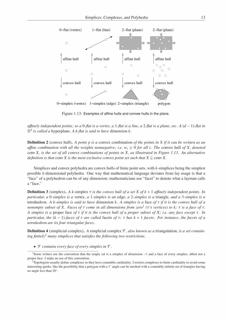
Figure 1.13: Examples of affine hulls and convex hulls in the plane.
affinely independent points; so a 0-flat is a vertex, a 1-flat is a line, a 2-flat is a plane, etc. A (d − 1)-flat inRd is called a hyperplane. A k-flat is said to have dimension k.
Definition 2 (convex hull). A point p is a convex combination of the points in X if it can be written as anaffine combination with all the weights nonnegative; i.e. wi ≥ 0 for all i. The convex hull of X, denotedconv X, is the set of all convex combinations of points in X, as illustrated in Figure 1.13. An alternativedefinition is that conv X is the most exclusive convex point set such that X ⊆ conv X.
Simplices and convex polyhedra are convex hulls of finite point sets, with k-simplices being the simplestpossible k-dimensional polyhedra. One way that mathematical language deviates from lay usage is that a“face” of a polyhedron can be of any dimension; mathematicians use “facet” to denote what a layman callsa “face.”
Definition 3 (simplex). A k-simplex τ is the convex hull of a set X of k + 1 affinely independent points. Inparticular, a 0-simplex is a vertex, a 1-simplex is an edge, a 2-simplex is a triangle, and a 3-simplex is atetrahedron. A k-simplex is said to have dimension k. A simplex is a face of τ if it is the convex hull of anonempty subset of X. Faces of τ come in all dimensions from zero1 (τ’s vertices) to k; τ is a face of τ.A simplex is a proper face of τ if it is the convex hull of a proper subset of X; i.e. any face except τ. Inparticular, the (k − 1)-faces of τ are called facets of τ; τ has k + 1 facets. For instance, the facets of atetrahedron are its four triangular faces.
Definition 4 (simplicial complex). A simplicial complex T , also known as a triangulation, is a set contain-ing finitely2 many simplices that satisfies the following two restrictions.
• T contains every face of every simplex in T .1Some writers use the convention that the empty set is a simplex of dimension −1 and a face of every simplex, albeit not a
proper face. I make no use of this convention.2Topologists usually define complexes so they have countable cardinality. I restrict complexes to finite cardinality to avoid some
interesting quirks, like the possibility that a polygon with a 1 angle can be meshed with a countably infinite set of triangles havingno angle less than 20.

14 Jonathan Richard Shewchuk
• For any two simplices σ, τ ∈ T , their intersection σ ∩ τ is either empty or a face of both σ and τ.
Convex polyhedra are as easy to define as simplices, but their faces are trickier. Whereas the convex hullof a subset of a simplex’s vertices is a face of the simplex, the convex hull of an arbitrary subset of a cube’svertices is usually not a face of the cube. The faces of a polyhedron are defined below in terms of supportinghyperplanes; observe that this definition is consistent with the definition of a face of a simplex above.
Definition 5 (convex polyhedron). A convex polyhedron is the convex hull of a finite point set. A polyhedronwhose affine hull is a k-flat is called a k-polyhedron and is said to have dimension k. A 0-polyhedron is avertex, a 1-polyhedron is an edge, and a 2-polyhedron is a polygon. The proper faces of a convex polyhedronC are the polyhedra that can be generated by taking the intersection of C with a hyperplane that intersectsC’s boundary but not C’s interior; such a hyperplane is called a supporting hyperplane of C. For example,the proper faces of a cube are six squares, twelve edges, and eight vertices. The faces of C are the properfaces of C and C itself. The facets of a k-polyhedron are its (k − 1)-faces.
A polyhedral complex imposes exactly the same restrictions as a simplicial complex.
Definition 6 (polyhedral complex). A polyhedral complex P is a set containing finitely many convex poly-hedra that satisfies the following two restrictions.
• P contains every face of every polyhedron in P.
• For any two polyhedra C,D ∈ P, their intersection C ∩ D is either empty or a face of both C and D.
Piecewise linear complexes are sets of polyhedra that are not necessarily convex. I call these polyhedralinear cells.
Definition 7 (linear cell). A linear k-cell is the union of a finite number of convex k-polyhedra, all includedin some common k-flat. A linear 0-cell is a vertex, a linear 2-cell is sometimes called a polygon, and a linear3-cell is sometimes called a polyhedron.
For k ≥ 1, a linear k-cell can have multiple connected components. These do no harm; removing alinear cell from a complex and replacing it with its connected components, or vice versa, makes no materialdifference. To simplify the exposition, I will forbid disconnected linear 1-cells in complexes; i.e. the onlylinear 1-cells are edges. For k ≥ 2, a linear cell can be only tenuously connected; e.g. a union of two squaresthat intersect at a single point is a linear 2-cell, even though it is not a simple polygon.
Another difference between linear cells and convex polyhedra is that we define the faces of a linear cellin a fundamentally different way that supports configurations like those in Figures 1.3 and 1.12. A linearcell’s faces are not an intrinsic property of the linear cell alone, but depend on the complex that contains it.I defer the details to Section 2.8.1, where I define piecewise linear complexes.
Piecewise smooth complexes are sets of cells called smooth cells, which are similar to linear cells exceptthat they are not linear, but are smooth manifolds.
A complex or a mesh is a representation of a domain. The former is a set of sets of points, and the latteris a set of points. The following operator collapses the former to the latter.
Definition 8 (underlying space). The underlying space of a complex P, denoted |P|, is the union of its cells;that is, |P| =
"
C∈PC.
Metric Space Topology 15
Ideally, a complex provided as input to a mesh generation algorithm and the mesh produced as outputshould cover exactly the same points. This ideal is not always possible—for example, if we are generatinga linear tetrahedral mesh of a curved domain. When it is achieved, we call it exact conformity.
Definition 9 (exact conformity). A complex T exactly conforms to a complex P if |T | = |P| and every cellin P is a union of cells in T . We also say that T is a subdivision of P.
1.4 Metric Space Topology
This section introduces basic notions from point set topology that underlie triangulations and other com-plexes. They are prerequisites for more sophisticated topological ideas—manifolds and homeomorphisms—introduced in Sections 1.6 and 1.7. A complex of linear elements cannot exactly conform to a curved domain,which raises the question of what it means for a triangulation to be a mesh of such a domain. To a layman,the word topology evokes visions of “rubber-sheet topology”: the idea that if you bend and stretch a sheetof rubber, it changes shape but always preserves the underlying structure of how it is connected to itself.Homeomorphisms offer a rigorous way to state that a mesh preserves the topology of a domain.
Topology begins with a set T of points—perhaps the points comprising the d-dimensional Euclideanspace Rd, or perhaps the points on the surface of a volume such as a coffee mug. We suppose that there is ametric d(p, q) that specifies the scalar distance between every pair of points p, q ∈ T. In the Euclidean spaceRd we choose the Euclidean distance. On the surface of the coffee mug, we could choose the Euclideandistance too; alternatively, we could choose the geodesic distance, namely the length of the shortest pathfrom p to q on the mug’s surface.
Let us briefly review the Euclidean metric. We write points in Rd as p = (p1, p2, . . . , pd), where each piis a real-valued coordinate. The Euclidean norm of a point p ∈ Rd is ∥p∥ =
#!di=1 p2
i$1/2, and the Euclidean
distance between two points p, q ∈ Rd is d(p, q) = ∥p − q∥ =#!d
i=1(pi − qi)2$1/2. I also use the notationd(·, ·) to express minimum distances between point sets P,Q ⊆ T,
d(p,Q) = infd(p, q) : q ∈ Q andd(P,Q) = infd(p, q) : p ∈ P, q ∈ Q.
The heart of topology is the question of what it means for a set of points—say, a squiggle drawn on apiece of paper—to be connected. After all, two distinct points cannot be adjacent to each other; they canonly be connected to another by an uncountably infinite bunch of intermediate points. Topologists solve thatmystery with the idea of limit points.
Definition 10 (limit point). Let Q ⊆ T be a point set. A point p ∈ T is a limit point of Q, also known as anaccumulation point of Q, if for every real number ϵ > 0, however tiny, Q contains a point q ! p such thatthat d(p, q) < ϵ.
In other words, there is an infinite sequence of points in Q that get successively closer and closer top—without actually being p—and get arbitrarily close. Stated succinctly, d(p,Q \ p) = 0. Observe that itdoesn’t matter whether p ∈ Q or not.
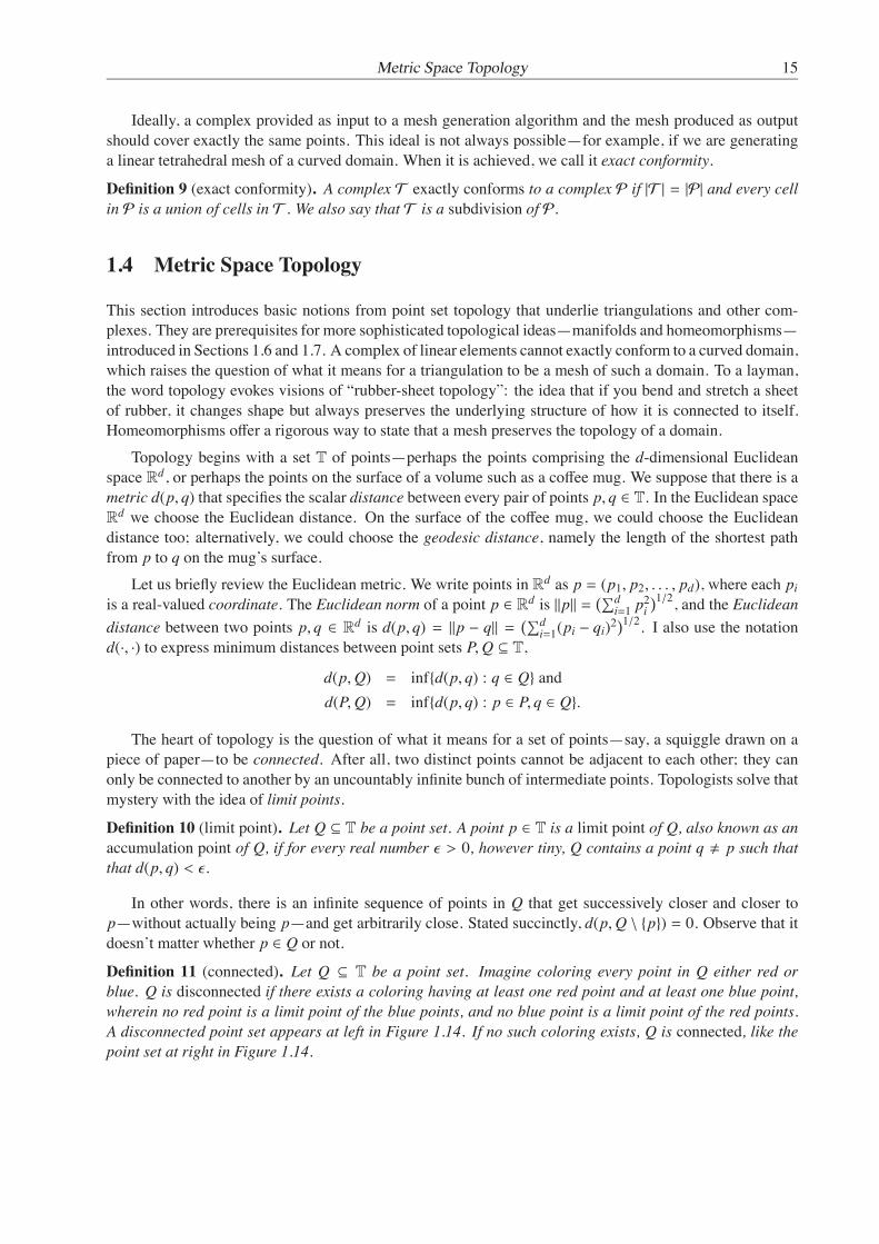
Definition 11 (connected). Let Q ⊆ T be a point set. Imagine coloring every point in Q either red orblue. Q is disconnected if there exists a coloring having at least one red point and at least one blue point,wherein no red point is a limit point of the blue points, and no blue point is a limit point of the red points.A disconnected point set appears at left in Figure 1.14. If no such coloring exists, Q is connected, like thepoint set at right in Figure 1.14.

16 Jonathan Richard Shewchuk
Figure 1.14: The disconnected point set at left can be partitioned into two connected subsets, which are coloreddifferently here. The point set at right is connected. The dark point at its center is a limit point of the lightly coloredpoints.
boundary/
boundaryinterior
closure
closure closure
closed open closed
interior ∅closure
closure
closed closed
∅
closure relative boundary
interiorrelative
openrelatively
boundary
interiorrelative
relative
boundary/boundary
Figure 1.15: Closed, open, and relatively open point sets in the plane. Dashed edges and open circles indicatepoints missing from the point set.
In these notes, I frequently distinguish between closed and open point sets. Informally, a triangle in theplane is closed if it contains all the points on its edges, and open if it excludes all the points on its edges, asillustrated in Figure 1.15. The idea can be formally extended to any point set.
Definition 12 (closure). The closure of a point set Q ⊆ T, denoted Cl Q, is the set containing every pointin Q and every limit point of Q. A point set Q is closed if Q = Cl Q, i.e. Q contains all its limit points. Thecomplement of a point set Q is T\Q. A point set Q is open if its complement is closed, i.e. T\Q = Cl (T\Q).
For example, let (0, 1) denote an open interval on the real number line—the set containing every r ∈ Rsuch that r > 0 and r < 1, and let [0, 1] denote a closed interval (0, 1) ∪ 0 ∪ 1. The numbers zero andone are both limit points of the open interval, so Cl (0, 1) = [0, 1] = Cl [0, 1]. Therefore, [0, 1] is closedand (0, 1) is not. The numbers zero and one are also limit points of the complement of the closed interval,R \ [0, 1], so (0, 1) is open, but [0, 1] is not.
The terminology is misleading because “closed” and “open” are not opposites. In every nonempty metricspace T, there are at least two point sets that are both closed and open: ∅ and T. The interval (0, 1] on thereal number line is neither open nor closed.
The definition of open set hides a subtlety that often misleads newcomers to point set topology: a triangleτ that is open in the metric space aff τ is not open in the metric space R3. Every point in τ is a limit point ofR3 \ τ, because you can find sequences of points that approach τ from the side. In recognition of this quirk,a simplex σ ⊂ Rd is said to be relatively open if it is open relative to its affine hull. It is commonplace toabuse terminology by writing “open simplex” for a simplex that is only relatively open, and I follow thisconvention in these notes. Particularly useful is the concept of an “open edge,” an edge that is missing itsendpoints, illustrated in Figure 1.15.
Informally, the boundary of a point set Q is the set of points where Q meets its complement T \ Q. Theinterior of Q contains all the other points of Q. Limit points provide formal definitions.
Definition 13 (boundary; interior). The boundary of a point set Q in a metric space T, denoted Bd Q, is

How to Measure an Element 17
the intersection of the closures of Q and its complement; i.e. Bd Q = Cl Q ∩ Cl (T \ Q). The interior of Q,denoted Int Q, is Q \ Bd Q = Q \ Cl (T \ Q).
For example, Bd [0, 1] = 0, 1 = Bd (0, 1) and Int [0, 1] = (0, 1) = Int (0, 1). The boundary of a triangle(closed or open) in the Euclidean plane is the union of the triangle’s three edges, and its interior is an opentriangle, illustrated in Figure 1.15. The terms boundary and interior have the same misleading subtlety asopen sets: the boundary of a triangle embedded in R3 is the whole triangle, and its interior is the empty set.Therefore, the relative boundary and relative interior of a simplex are its boundary and interior relative to itsaffine hull rather than the entire Euclidean space. Again, I often abuse terminology by writing “boundary”for relative boundary and “interior” for relative interior.
Definition 14 (bounded; compact). The diameter of a point set Q is supp,q∈Q d(p, q). The set Q is boundedif its diameter is finite, or unbounded if its diameter is infinite. A point set Q in a metric space is compact ifit is closed and bounded.
Besides simplices and polyhedra, the point sets we use most in these notes are balls and spheres.
Definition 15 (Euclidean ball). In Rd, the Euclidean d-ball with center c and radius r, denoted B(c, r),is the point set B(c, r) = p ∈ Rd : d(p, c) ≤ r. A 1-ball is an edge, and a 2-ball is sometimes calleda disk. A unit ball is a ball with radius 1. The boundary of the d-ball is called the Euclidean (d − 1)-sphere and denoted S (c, r) = p ∈ Rd : d(p, c) = r. For example, a circle is a 1-sphere, and a layman’s“sphere” in R3 is a 2-sphere. If we remove the boundary from a ball, we have the open Euclidean d-ballBo(c, r) = p ∈ Rd : d(p, c) < r.
The foregoing text introduces point set topology in terms of metric spaces. Surprisingly, it is possible todefine all the same concepts without the use of a metric, point coordinates, or any scalar values at all. Topo-logical spaces are a mathematical abstraction for representing the topology of a point set while excludingall information that is not topologically essential. In these notes, all the topological spaces have metrics.
1.5 How to Measure an Element
Here, I describe ways to measure the size, angles, and quality of a simplicial element, and I introduce somegeometric structures associated with simplices—most importantly, their circumspheres and circumcenters.
Definition 16 (circumsphere). Let τ be a simplex embedded in Rd. A circumsphere, or circumscribingsphere, of τ is a (d − 1)-sphere whose boundary passes through every vertex of τ, illustrated in Figure 1.16.A circumball, or circumscribing ball, of τ is a d-ball whose boundary is a circumsphere of τ. A closed cir-cumball includes its boundary—the circumsphere—and an open circumball excludes it. If τ is a k-simplex,the k-circumball of τ is the unique k-ball whose boundary passes through every vertex of τ, and its rel-ative boundary is the (k − 1)-circumsphere of τ. I sometimes call a 2-circumball a circumdisk and a 1-circumsphere a circumcircle.
If τ is a d-simplex in Rd, it has one unique circumsphere and circumball; but if τ has dimension less thand, it has an infinite set of circumspheres and circumballs. Consider a triangle τ in R3, for example. There isonly one circumcircle of τ, which passes through τ’s three vertices, but τ has infinitely many circumspheres,and the intersection of any of those circumspheres with τ’s affine hull is τ’s circumcircle. The smallestof these circumspheres is special, because its center lies on τ’s affine hull, it has the same radius as τ’scircumcircle, and τ’s circumcircle is its equatorial cross-section. Call τ’s smallest circumcircle, illustratedin Figure 1.17, its diametric circle; and call τ’s smallest circumdisk its diametric disk.

18 Jonathan Richard Shewchuk
min−containment ball
rRr
circumball inball
mc
Figure 1.16: Three spheres associated with a triangle.
Figure 1.17: A triangle, two circumspheres of the triangle of which the smaller (solid) is the triangle’s diamet-ric sphere, the triangle’s circumcircle (the equatorial cross-section of the diametric sphere), and the triangle’scircumcenter.
Definition 17 (diametric sphere). The diametric sphere of a simplex τ is the circumsphere of τ with thesmallest radius, and the diametric ball of τ is the circumball of τ with the smallest radius, whose boundaryis the diametric sphere. The circumcenter of τ is the point at the center of τ’s diametric sphere, which alwayslies on aff τ. The circumradius of τ is the radius of τ’s diametric sphere.
The significance of circumcenters in Delaunay refinement algorithms is that the best place to insert anew vertex into a mesh is often at the circumcenter of a poorly shaped element, domain boundary triangle,or domain boundary edge. In a Delaunay mesh, these circumcenters are locally far from other mesh vertices,so inserting them does not create overly short edges.
Other spheres associated with simplicial elements are the insphere and the min-containment sphere, bothillustrated in Figure 1.16.
Definition 18 (insphere). The inball, or inscribed ball, of a k-simplex τ is the largest k-ball B ⊂ τ. Observethat B is tangent to every facet of τ. The insphere of τ is the boundary of B, the incenter of τ is the point atthe center of B, and the inradius of τ is the radius of B.
Definition 19 (min-containment sphere). The min-containment ball, or minimum enclosing ball, of a k-simplex τ is the smallest k-ball B ⊃ τ. The min-containment ball is always a diametric ball of a face of τ.The min-containment sphere of τ is the boundary of B.
Finite element practitioners often represent the size of an element by the length of its longest edge, butone could argue that the radius of its min-containment sphere is a slightly better measure, because there aresharp error bounds for piecewise linear interpolation over simplicial elements that are directly proportionalto the squares of the radii of their min-containment spheres. Details appear in Section 4.4.

How to Measure an Element 19
Needle Cap
Figure 1.18: Skinny triangles have circumdisks larger than their shortest edges.
A quality measure is a mapping from elements to scalar values that estimates the suitability of an el-ement’s shape independently of its size. The most obvious quality measures of a triangle are its smallestand largest angles, and a tetrahedron can be judged by its dihedral angles. I denote the angle between twovectors u and v as
∠(u, v) = arccosu · v|u||v| .
I compute an angle ∠xyz of a triangle as ∠(x − y, z − y).
A dihedral angle is a measure of the angle separating two planes or polygons in R3—for example, thefacets of a tetrahedron or 3-polyhedron. Suppose that two flat facets meet at an edge yz, where y and z arepoints in R3. Let w be a point lying on one of the facets, and let x be a point lying on the other. It is helpfulto imagine the tetrahedron wxyz. The dihedral angle separating the two facets is the same angle separatingwyz and xyz, namely ∠(u, v) where u = (y − w) × (z − w) and v = (y − x) × (z − x) are vectors normal towyz and xyz.
Elements can go bad in different ways, and it is useful to distinguish types of skinny elements. There aretwo kinds of skinny triangles, illustrated in Figure 1.18: needles, which have one edge much shorter than theothers, and caps, which have an angle near 180 and a large circumdisk. Figure 1.19 offers a taxonomy oftypes of skinny tetrahedra. The tetrahedra in the top row are skinny in one dimension and fat in two. Thosein the bottom row are skinny in two dimensions and fat in one. Spears, spindles, spades, caps, and slivershave a dihedral angle near 180; the others may or may not. Spikes, splinters, and all the tetrahedra in thetop row have a dihedral angle near 0; the others may or may not. The cap, which has a vertex quite close tothe center of the opposite triangle, is notable for a large solid angle, near 360. Spikes also can have a solidangle arbitrarily close to 360, and all the skinny tetrahedra can have a solid angle arbitrarily close to zero.
There are several surprises. The first is that spires, despite being skinny, can have all their dihedral anglesbetween 60 and 90, even if two edges are separated by a plane angle near 0. Spires with good dihedralangles are harmless in many applications, and are indispensable at the tip of a needle-shaped domain, butsome applications eschew them anyway. The second surprise is that a spear or spindle tetrahedron can havea dihedral angle near 180 without having a small dihedral angle. By contrast, a triangle with an angle near180 must have an angle near 0.
For many purposes—mesh improvement, for instance—it is desirable to have a single quality measurethat punishes both angles near 0 and angles near 180, and perhaps spires as well. Most quality measuresare designed to reach one extreme value for an equilateral triangle or tetrahedron, and an opposite extremevalue for a degenerate element—a triangle whose vertices are collinear, or a tetrahedron whose verticesare coplanar. In these notes, the most important quality measure is the radius-edge ratio, because it is

20 Jonathan Richard Shewchuk
wedge spade cap
spire spear spindle spike splinter
sliver
Figure 1.19: A taxonomy of skinny tetrahedra, adapted from Cheng, Dey, Edelsbrunner, Facello, and Teng [29].
naturally bounded by Delaunay refinement algorithms (a fact first pointed out by Miller, Talmor, Teng, andWalkington [81]).
Definition 20 (radius-edge ratio). The radius-edge ratio of a simplex τ is R/ℓmin, where R is τ’s circumradiusand ℓmin is the length of its shortest edge.
We would like the radius-edge ratio to be as small as possible; it ranges from ∞ for most degeneratesimplices down to 1/
√3 " 0.577 for an equilateral triangle or
√6/4 " 0.612 for an equilateral tetrahedron.
But is it a good estimate of element quality?
In two dimensions, the answer is yes. A triangle’s radius-edge ratio is related to its smallest angle θminby the formula
Rℓmin=
12 sin θmin
.
Figure 1.20 illustrates how this identity is derived for a triangle xyz with circumcenter c. Observe that thetriangles ycz and xcz are isosceles, so their apex angles are ∠ycz = 180 − 2φ and ∠xcz = 180 − 2φ − 2θ.Therefore, ϕ = 2θmin and ℓmin = 2R sin θmin. This reasoning holds even if φ is negative.
The smaller a triangle’s radius-edge ratio, the larger its smallest angle. The angles of a triangle sum to180, so the triangle’s largest angle is at most 180 − 2θmin; hence an upper bound on the radius-edge ratioplaces bounds on both the smallest and largest angles.
In three dimensions, however, the radius-edge ratio is a flawed measure. It screens out all the tetrahedrain Figure 1.19 except slivers. A degenerate sliver can have a radius-edge ratio as small as 1/
√2 " 0.707,
which is not far from the 0.612 of an equilateral tetrahedron. Delaunay refinement algorithms are guaranteedto remove all tetrahedra with large radius-edge ratios, but they do not promise to remove all slivers.
There are other quality measures that screen out all the skinny tetrahedra in Figure 1.19, includingslivers and spires, but Delaunay refinement does not promise to bound these measures. A popular measureis the radius ratio r/R, suggested by Cavendish, Field, and Frey [25], where r is τ’s inradius and R isits circumradius. It obtains a maximum value of 1/2 for an equilateral triangle or 1/3 for an equilateraltetrahedron, and a minimum value of zero for a degenerate element, which implies that it approaches zero

Maps and Homeomorphisms 21
θ + φ
R
c
R
z
θφ
φϕ
ℓmin yx
R
Figure 1.20: Relationships between the circumradius R, shortest edge ℓmin, and smallest angle θ.
as any dihedral angle separating τ’s faces approaches 0 or 180, any plane angle separating τ’s edgesapproaches 0 or 180, or any solid angle at τ’s vertices approaches 0 or 360.
For a triangle τ, the radius ratio is related to the smallest angle θmin by the inequalities
2 sin2 θmin2≤
rR≤ 2 tan
θmin2,
which implies that it approaches zero as θmin approaches zero, and vice versa.
Two unfortunate properties of the circumradius are that it is relatively expensive to compute for a tetra-hedron, and it can be numerically unstable. A tiny perturbation of the position of one vertex of a skinnytetrahedron can induce an arbitrarily large change in its circumradius. Both the radius-edge ratio and theradius ratio inherit these problems. In these respects, a better quality measure for tetrahedra is the volume-length measure V/ℓ3rms, suggested by Parthasarathy, Graichen, and Hathaway [90], where V is the volumeof a tetrahedron and ℓrms is the root-mean-squared length of its six edges. It obtains a maximum valueof 1/(6
√2) for an equilateral tetrahedron and a minimum value of zero for a degenerate tetrahedron. The
volume-length measure is numerically stable and faster to compute than a tetrahedron’s circumradius. It hasproven itself as a filter against all poorly shaped tetrahedra and as an objective function for mesh improve-ment algorithms, especially optimization-based smoothing [70].
1.6 Maps and Homeomorphisms
Two metric spaces are considered to be the same if the points that comprise them are connected the sameway. For example, the boundary of a cube can be deformed into a sphere without cutting or gluing it. Theyhave the same topology. We formalize this notion of topological equality by defining a function that mapsthe points of one space to points of the other and preserves how they are connected. Specifically, the functionpreserves limit points.
A function from one space to another that preserves limit points is called a continuous function or amap.3 Continuity is just a step on the way to topological equivalence, because a continuous function can
3There is a small caveat with this characterization: a function g that maps a neighborhood of x to a single point g(x) may be

22 Jonathan Richard Shewchuk
(a) (b)
(c) (d)
Figure 1.21: (a) A 1-ball. (b) Spaces homeomorphic to the 1-sphere. (c) Spaces homeomorphic to the 2-ball.(d) An open 2-ball. It is homeomorphic to R2, but not to a closed 2-ball.
map many points to a single point in the target space, or map no points to a given point in the target space.True equivalence is marked by a homeomorphism, a one-to-one function from one space to another thatpossesses both continuity and a continuous inverse, so that limit points are preserved in both directions.
Definition 21 (continuous function; map). Let T and U be metric spaces. A function g : T → U iscontinuous if for every set Q ⊆ T and every limit point p ∈ T of Q, g(p) is either a limit point of the set g(Q)or in g(Q). Continuous functions are also called maps.
Definition 22 (homeomorphism). Let T and U be metric spaces. A homeomorphism is a bijective (one-to-one) map h : T → U whose inverse is continuous too. Two metric spaces are homeomorphic if there existsa homeomorphism between them.
Homeomorphism induces an equivalence relation among metric spaces, which is why two homeomor-phic metric spaces are called topologically equivalent. Figure 1.21(b, c) shows pairs of metric spaces thatare homeomorphic. A less obvious example is that the open unit d-ball Bd
o = x ∈ Rd : |x| < 1 is homeo-morphic to the Euclidean space Rd, a fact demonstrated by the map h(p) = (1/(1 − |p|))p. The same mapshows that the open unit halfball Hd = x ∈ Rd : |x| < 1 and xd ≥ 0 is homeomorphic to the Euclideanhalfspace x ∈ Rd : xd ≥ 0.
Homeomorphism gives us a purely topological definition of what it means to triangulate a domain.
Definition 23 (triangulation of a metric space). A simplicial complexK is a triangulation of a metric spaceT if its underlying space |K| is homeomorphic to T.
1.7 Manifolds
A manifold is a set of points that is locally connected in a particular way. A 1-manifold has the structure ofa piece of string, possibly with its ends tied in a loop, and a 2-manifold has the structure of a piece of paper
continuous, but technically g(x) is not a limit point of itself, so in this sense a continuous function might not preserve all limitpoints. This technicality does not apply to homeomorphisms because they are bijective.

Manifolds 23
Figure 1.22: Mobius band.
or rubber sheet that has been cut and perhaps glued along its edges—a category that includes disks, spheres,tori, and Mobius bands.
Definition 24 (manifold). A metric space Σ is a k-manifold, or simply manifold, if every point x ∈ Σ has aneighborhood homeomorphic to Rk or Hk. The dimension of Σ is k.
A manifold can be viewed as a purely abstract metric space, or it can be embedded into a metric spaceor a Euclidean space. Even without an embedding, every manifold can be partitioned into boundary andinterior points. Observe that these words mean very different things for a manifold than they do for a metricspace.
Definition 25 (boundary, interior). The interior IntΣ of a manifold Σ is the set of points in Σ that have aneighborhood homeomorphic to Rk. The boundary BdΣ of Σ is the set of points Σ \ IntΣ. Except for thecase of 0-manifolds (points) whose boundary is empty, BdΣ consists of points that have a neighborhoodhomeomorphic to Hk. If BdΣ is the empty set, we say that Σ is without boundary.
For example, the closed disk B2 is a 2-manifold whose interior is the open disk B2o and whose boundary
is the circle S1. The open disk B2o is a 2-manifold whose boundary is the empty set. So is the Euclidean space
R2, and so is the sphere S2. The open disk is homeomorphic to R2, but the sphere is topologically differentfrom the other two. Moreover, the sphere is compact (bounded and closed with respect to R3) whereas theother two are not.
A 2-manifold Σ is non-orientable if starting from a point p one can walk on Σ and end up on theopposite side of Σ when returning to p. Otherwise, Σ is orientable. Spheres and balls are orientable, whereasthe Mobius band in Figure 1.22 is a non-orientable 2-manifold.
A surface is a 2-manifold that is a subspace of Rd. Any compact surface without boundary in R3 isan orientable 2-manifold. To be non-orientable, a compact surface must have a nonempty boundary or beembedded in a 4- or higher-dimensional Euclidean space.
A surface can sometimes be disconnected by removing one or more loops (1-manifolds without bound-ary) from it. The genus of a surface is g if 2g is the maximum number of loops that can be removed fromthe surface without disconnecting it; here the loops are permitted to intersect each other. For example, thesphere has genus zero as any loop cuts it into two surfaces. The torus has genus one: a circular cut aroundits neck and a second circular cut around its circumference, illustrated in Figure 1.23(a), allow it to unfoldinto a rectangle, which topologically is a disk. A third loop would cut it into two pieces. Figure 1.23(b)shows a 2-manifold without boundary of genus 2. Although a high-genus surface can have a very complexshape, all compact 2-manifolds of genus g without boundary are homeomorphic to each other.

24 Jonathan Richard Shewchuk
(a) (b)
Figure 1.23: (a) Removal of the bold loops opens up the torus into a topological disk. (b) Every surface withoutboundary in R3 resembles a sphere or a conjunction of one or more tori.

Chapter 2
Two-Dimensional Delaunay Triangulations
The Delaunay triangulation is a geometric structure that engineers have used for meshes since mesh gener-ation was in its infancy. In two dimensions, it has a striking advantage: among all possible triangulationsof a fixed set of points, the Delaunay triangulation maximizes the minimum angle. It also optimizes severalother geometric criteria related to interpolation accuracy. If it is your goal to create a triangulation withoutsmall angles, it seems almost silly to consider a triangulation that is not Delaunay. Delaunay triangulationshave been studied thoroughly, and excellent algorithms are available for constructing and updating them.
A constrained triangulation is a triangulation that enforces the presence of specified edges—for example,the boundary of a nonconvex object. A constrained Delaunay triangulation relaxes the Delaunay propertyjust enough to recover those edges, while enjoying optimality properties similar to those of a Delaunaytriangulation. Constrained Delaunay triangulations are nearly as popular as their unconstrained ancestors.
This chapter surveys two-dimensional Delaunay triangulations, constrained Delaunay triangulations,and their geometric properties. See Fortune [52] for an alternative survey of Delaunay triangulations, andAurenhammer [4] for a survey of many more types of Voronoi diagrams.
Figure 2.1: A Delaunay triangulation.
25

26 Jonathan Richard Shewchuk
Figure 2.2: Incremental construction of a lexicographic triangulation.
2.1 Triangulations of a Planar Point Set
The word triangulation usually refers to a simplicial complex, but it has multiple meanings when we discussa triangulation of some geometric entity that is being triangulated. There are triangulations of point sets,polygons, polyhedra, and many other structures. Consider points in the plane (or in any Euclidean space).
Definition 26 (triangulation of a point set). Let V (for “vertices”) be a finite set of points in the plane. Atriangulation of V is a simplicial complex T such that
• V is the set of vertices in T , and
• the union of all the simplices in T is the convex hull of V.
Does every point set have a triangulation? Yes. Consider the lexicographic triangulation illustrated inFigure 2.2. To construct one, sort the points lexicograpically (that is, by x-coordinate, ordering points withthe same x-coordinate according to their y-coordinates), yielding a sorted sequence v1, v2, . . . , vn of points.Define the lexicographic triangulation Ti of the first i points by induction as follows. The first triangulationis T1 = v1. Each subsequent triangulation is Ti = Ti−1 ∪ vi ∪ conv(vi ∪ σ) : σ ∈ Ti−1 and the relativeinterior of conv(vi ∪ σ) intersects no simplex in Ti−1.
V has a triangulation even if all its points are collinear: Tn contains n vertices, n − 1 collinear edgesconnecting them, and no triangles.
A triangulation of n points in the plane has at most 2n − 5 triangles and 3n − 6 edges as a consequenceof Euler’s formula. With no change, Definition 26 defines triangulations of point sets in higher-dimensionalEuclidean spaces as well.
2.2 The Delaunay Triangulation
The Delaunay triangulation of a point set V , introduced by Boris Nikolaevich Delone [43] in 1934, is atriangulation of V whose triangles are particularly nicely shaped. Figure 2.1 illustrates a Delaunay triangu-lation. Its defining characteristic is the empty circumcircle property: no triangle has a circumscribing circlethat encloses any point in V .
Definition 27 (circumcircle). The circumcircle, or circumscribing circle, of a triangle is the unique circlethat passes through all three of its vertices. A circumcircle of an edge is any circle that passes through bothits vertices.
In the plane, an edge has an infinite set of circumcircles; a triangle has only one.

The Delaunay Triangulation 27
Figure 2.3: Every triangle in a Delaunay triangulation has an empty circumcircle.
(a) (b) (c)
Figure 2.4: Three ways to define a Delaunay structure in the presence of cocircular vertices. (a) Include all theDelaunay simplices. (b) Choose a subset of Delaunay simplices that comprises a triangulation. (c) Exclude allcrossing Delaunay edges, and fuse overlapping Delaunay triangles into Delaunay polygons.
Definition 28 (Delaunay). In the context of a finite point set V, a triangle is Delaunay if its vertices are in Vand its circumcircle is empty—encloses no point in V. Note that any number of points can lie on a Delaunaytriangle’s circumcircle.
An edge is Delaunay if its vertices are in V and it has at least one empty circumcircle.
A Delaunay triangulation of V, denoted Del V, is a triangulation of V in which every triangle is Delau-nay, as illustrated in Figure 2.3.
You might wonder whether every point set has a Delaunay triangulation, and how many Delaunay trian-gulations a point set can have. The answer to the first question is “yes.” Section 2.3 gives some intuition forwhy this is true, and Section 2.4 gives a proof.
The Delaunay triangulation of V is unique if and only if no four points in V lie on a common emptycircle, a fact proven in Section 2.7. Otherwise, there are Delaunay triangles and edges whose interiorsintersect, as illustrated in Figure 2.4(a). Most applications omit some of these triangles and edges so thatthe survivors form a simplicial complex, as in Figure 2.4(b). Depending on which Delaunay simplices youkeep and which you discard, you obtain different Delaunay triangulations.
It is sometimes useful to unite the intersecting triangles into a single polygon, depicted in Figure 2.4(c).The Delaunay subdivision obtained this way is a polyhedral complex, rather than a simplicial complex. Ithas the advantage of being the geometric dual of the famous Voronoi diagram.
Clearly, a simplex’s being Delaunay does not guarantee that it is in every Delaunay triangulation of apoint set. But a slightly stronger property does provide that guarantee.

28 Jonathan Richard Shewchuk
Figure 2.5: Every edge on the boundary of a convex triangulation is strongly Delaunay, because it is alwayspossible to find an empty circle that passes through its endpoints and no other vertex.
Definition 29 (strongly Delaunay). In the context of a finite point set V, a triangle τ is strongly Delaunay ifits vertices are in V and no point in V lies inside or on its circumcircle, except the vertices of τ.
An edge e is strongly Delaunay if its vertices are in V and it has at least one circumcircle that no pointin V lies inside or on, except the vertices of e.
Every point in V is a strongly Delaunay vertex.
Every Delaunay triangulation of V contains every strongly Delaunay simplex, a fact proven in Sec-tion 2.7. The Delaunay subdivision contains the strongly Delaunay edges and triangles, and no others.
Consider two examples of strongly Delaunay edges. First, every edge on the boundary of a triangulationof V is strongly Delaunay. Figure 2.5 shows why. Second, the edge connecting a point v ∈ V to its nearestneighbor w ∈ V is strongly Delaunay, because the smallest circle passing through v and w does not enclosenor touch any other point in V . Therefore, every Delaunay triangulation connects every vertex to its nearestneighbor.
2.3 The Parabolic Lifting Map
Given a finite point set V , the parabolic lifting map of Seidel [107, 48] transforms the Delaunay subdivisionof V into faces of a convex polyhedron in three dimensions, as illustrated in Figure 2.6. This relationshipbetween Delaunay triangulations and convex hulls has two consequences. First, it makes many properties ofthe Delaunay triangulation intuitive. For example, from the fact that every finite point set has a polyhedralconvex hull, it follows that every finite point set has a Delaunay triangulation. Second, it brings to meshgeneration the power of a huge literature on polytope theory and algorithms: every convex hull algorithm isa Delaunay triangulation algorithm!
The parabolic lifting map sends each point p = (x, y) ∈ E2 to a point p+ = (x, y, x2 + y2) ∈ E3. Call p+the lifted companion of p.
Consider the convex hull conv(V+) of the lifted points V+ = v+ : v ∈ V. Figure 2.6 illustrates itsdownward-facing faces. Formally, a face f of conv(V+) is downward-facing if no point in conv(V+) isdirectly below any point in f , with respect to the z-axis. Call the collection of downward-facing faces theunderside of conv(V+). Projecting the underside of conv(V+) to the x-y plane (by discarding every point’sz-coordinate) yields the Delaunay subdivision of V . If V has more than one Delaunay triangulation, thisDelaunay subdivision has non-triangular polygons, like the hexagon in Figure 2.4(c). Triangulating thesepolygonal faces yields a Delaunay triangulation.
For a simplex σ in the plane, its lifted companion σ+ is the simplex embedded in E3 whose vertices arethe lifted companions of the vertices of σ. Note that σ+ is flat, and does not curve to hug the paraboloid.The following lemma and theorem show that every Delaunay simplex’s lifted companion is included in adownward-facing face of conv(V+).

The Parabolic Lifting Map 29
Vy
x
z
+V
Figure 2.6: The parabolic lifting map.
Lemma 1. Let C be a circle in the plane. Let C+ = p+ : p ∈ C be the ellipse obtained by lifting C tothe paraboloid. Then the points of C+ lie on a plane h, which is not parallel to the z-axis. Furthermore,every point p inside C lifts to a point p+ below h, and every point p outside C lifts to a point p+ above h.Therefore, testing whether a point p is inside, on, or outside C is equivalent to testing whether the liftedpoint p+ is below, on, or above h.
Proof. Let O and r be the center and radius of C, respectively. Let p be a point in the plane. The z-coordinateof p+ is |p|2. By expanding |O − p|2, we have the identity |p|2 = 2O · p − |O|2 + |O − p|2.
With O and r fixed and p ∈ E2 varying, the equation z = 2O · p − |O|2 + r2 defines a plane h in E3, notparallel to the z-axis. For every point p ∈ C, |O − p| = r, so C+ ⊂ h. For every point p # C, if |O − p| < r,then the lifted point p+ lies below h, and if |O − p| > r, then p+ lies above h. "
Theorem 2 (Seidel [107]). Let σ be a simplex whose vertices are in V, and let σ+ be its lifted companion.Then σ is Delaunay if and only if σ+ is included in some downward-facing face of conv(V+). The simplexσ is strongly Delaunay if and only if σ+ is a downward-facing face of conv(V+).
Proof. If σ is Delaunay, σ has a circumcircle C that encloses no point in V . Let h be the unique plane in E3
that includes C+. By Lemma 1, no point in V+ lies below h. Because the vertices of σ+ are in C+, h ⊃ σ+.Therefore, σ+ is included in a downward-facing face of the convex hull of V+. If σ is strongly Delaunay,every point in V+ lies above h except the vertices of σ+. Therefore, σ+ is a downward-facing face of theconvex hull of V+.
The converse implications follow by reversing the argument. "
The parabolic lifting map works equally well for Delaunay triangulations in three or more dimensions;Lemma 1 and Theorem 2 generalize to higher dimensions without any new ideas. Theorem 2 implies that

30 Jonathan Richard Shewchuk
e e
Figure 2.7: At left, e is locally Delaunay. At right, e is not.
any algorithm for constructing convex hulls of point sets in Ed+1 can construct the Delaunay triangulationof a point set in Ed.
The relationship between Delaunay triangulations and convex hulls was first discovered by Brown [21],who proposed a different lifting map that projects V onto a sphere. The parabolic lifting map is numericallybetter behaved than the spherical one.
2.4 The Delaunay Lemma
Perhaps the most important result about Delaunay triangulations is the Delaunay Lemma, proven by BorisDelaunay himself [43]. It provides an alternative characterization of the Delaunay triangulation: a triangu-lation whose edges are locally Delaunay.
Definition 30 (locally Delaunay). Let e be an edge in a triangulation T of a planar point set. If e is anedge of fewer than two triangles in T , then e is said to be locally Delaunay. If e is an edge of exactly twotriangles τ1 and τ2 in T , then e is locally Delaunay if it has a circumcircle enclosing no vertex of τ1 nor τ2.Equivalently, the circumcircle of τ1 encloses no vertex of τ2. Equivalently, the circumcircle of τ2 enclosesno vertex of τ1.
Figure 2.7 shows two different triangulations of six vertices. In the triangulation at left, the edge e islocally Delaunay, because the depicted circumcircle of e does not enclose either vertex opposite e. Never-theless, e is not Delaunay, thanks to other vertices inside e’s circumcircle. In the triangulation at right, e isnot locally Delaunay; every circumcircle of e encloses at least one of the two vertices opposite e.
The Delaunay Lemma has several uses. First, it provides a linear-time algorithm to determine whethera triangulation is Delaunay: simply test whether every edge is locally Delaunay. Second, it implies a simplealgorithm for producing a Delaunay triangulation called the flip algorithm (Section 2.5). The flip algorithmhelps to prove that Delaunay triangulations have useful optimality properties. Third, the Delaunay Lemmahelps to prove the correctness of other algorithms for constructing Delaunay triangulations.
As with many properties of Delaunay triangulations, the lifting map provides intuition for the DelaunayLemma. On the lifting map, the Delaunay Lemma is essentially the observation that a simple polyhedronis convex if and only if its has no reflex edge. A reflex edge is an edge where the polyhedron is locallynonconvex; that is, the dihedral angle at which the two adjoining faces meet along that edge exceeds 180,measured through the interior of the polyhedron. If a triangulation has an edge that is not locally Delaunay,that edge’s lifted companion is a reflex edge of the lifted triangulation (by Lemma 1).
Theorem 3 (Delaunay Lemma [43]). Let T be a triangulation of a point set V. The following three state-ments are equivalent.

The Delaunay Lemma 31
4
4
2
v = w
w
w
τ
e1
2e1
3 w
τ2τ1
τ3e4e3
τ
e
v
τ
wτ
1
1
1
(a) (b)
Figure 2.8: (a) Because τ’s circumcircle encloses v, some edge between v and τ is not locally Delaunay. (b) Be-cause v lies above e1 and inside τ’s circumcircle, and because w1 lies outside (or on) τ’s circumcircle, v must lieinside τ1’s circumcircle.
A. Every triangle in T is Delaunay (i.e. T is Delaunay).
B. Every edge in T is Delaunay.
C. Every edge in T is locally Delaunay.
Proof. If the points in V are all collinear, V has only one triangulation, which trivially satisfies all threeproperties.
Otherwise, let e be an edge in T ; e is an edge of at least one triangle τ ∈ T . If τ is Delaunay, τ’scircumcircle is empty, and because τ’s circumcircle is also a circumcircle of e, e is Delaunay. Therefore,Property A implies Property B. If an edge is Delaunay, it is clearly locally Delaunay too, so Property Bimplies Property C. The proof is complete if Property C implies Property A. Of course, this is the hard part.
Suppose that every edge in T is locally Delaunay. Suppose for the sake of contradiction that Property Adoes not hold. Then some triangle τ ∈ T is not Delaunay, and some vertex v ∈ V is inside τ’s circumcircle.Let e1 be the edge of τ that separates v from the interior of τ, as illustrated in Figure 2.8(a). Without loss ofgenerality, assume that e1 is oriented horizontally, with τ below e1.
Draw a line segment from the midpoint of e1 to v—see the dashed line in Figure 2.8(a). If the linesegment intersects some vertex other than v, replace v with the lowest such vertex. Let e1, e2, e3, . . ., em bethe sequence of triangulation edges (from bottom to top) whose relative interiors the line segment intersects.Because T is a triangulation of V , every point on the line segment lies either in a single triangle or on anedge. Let wi be the vertex above ei that forms a triangle τi in conjunction with ei. Observe that wm = v.
By assumption, e1 is locally Delaunay, so w1 lies on or outside the circumcircle of τ. As Figure 2.8(b)shows, it follows that the circumcircle of τ1 encloses every point above e1 inside the circumcircle of τ, andhence encloses v. Repeating this argument inductively, we find that the circumcircles of τ2, . . . , τm enclosev. But wm = v is a vertex of τm, which contradicts the claim that v is inside the circumcircle of τm. "

32 Jonathan Richard Shewchuk
e
Figure 2.9: In this nonconvex quadrilateral, e cannot be flipped.
e
v
w
C
v
C
w
e
(a) (b)
Figure 2.10: (a) The edge e is locally Delaunay. (b) The edge e is not locally Delaunay. The edge created by aflip of e is locally Delaunay.
2.5 The Flip Algorithm
The flip algorithm has at least three uses: it is a simple algorithm for computing a Delaunay triangulation, itis the core of a constructive proof that every finite set of points in the plane has a Delaunay triangulation, andit is the core of a proof that the Delaunay triangulation optimizes several geometric criteria when comparedwith all other triangulations of the same point set.
Let V be a point set you wish to triangulate. The flip algorithm begins with any triangulation T of V;for instance, the lexicographic triangulation described in Section 2.1. The Delaunay Lemma tells us that Tis Delaunay if and only if every edge in T is locally Delaunay. The flip algorithm repeatedly chooses anyedge that is not locally Delaunay, and flips it.
The union of two triangles that share an edge is a quadrilateral, and the shared edge is a diagonal ofthe quadrilateral. To flip an edge is to replace it with the quadrilateral’s other diagonal, as illustrated inFigure 2.7. An edge flip is legal only if the two diagonals cross each other—equivalently, if the quadrilateralis convex. Figure 2.9 shows that not every edge can be flipped, because the quadrilateral might not beconvex. Fortunately, unflippable edges are always locally Delaunay.
Lemma 4. Let e be an edge in a triangulation of V. Either e is locally Delaunay, or e is flippable and theedge created by flipping e is locally Delaunay.
Proof: Let v and w be the vertices opposite e. Consider the quadrilateral defined by e, v, and w, illustratedin Figure 2.10. Let C be the circle that passes through v and the vertices of e.
If w is on or outside C, as in Figure 2.10(a), then the empty circle C demonstrates that e is locallyDelaunay.
Otherwise, w is inside the section of C bounded by e and opposite v. This section is shaded in Fig-ure 2.10(b). The quadrilateral is thus strictly convex, so e is flippable. Furthermore, the circle that is tangent

The Flip Algorithm 33
to C at v and passes through w does not enclose the endpoints of e, because C encloses it, as Figure 2.10(b)demonstrates. Therefore, the edge vw is locally Delaunay. "
Lemma 4 shows that the flip algorithm can flip any edge that is not locally Delaunay, thereby creating anedge that is. Unfortunately, the outer four edges of the quadrilateral might discover that they are no longerlocally Delaunay, even if they were locally Delaunay before the flip. If the flip algorithm repeatedly flipsedges that are not locally Delaunay, will it go on forever?
Theorem 5. Given a triangulation of n points, the flip algorithm terminates after O(n2) edge flips, yieldinga Delaunay triangulation.
Proof: Let T be the initial triangulation provided as input to the flip algorithm. Let T + = σ+ : σ ∈ T bethe initial triangulation lifted to the parabolic lifting map; T + is a simplicial complex embedded in E3. If Tis Delaunay, then T + triangulates the underside of conv(V+); otherwise, by Lemma 1, the edges of T thatare not locally Delaunay lift to reflex edges of T +.
By Lemma 4, an edge flip replaces an edge that is not locally Delaunay with one that is. In the liftedtriangulation T +, a flip replaces a reflex edge with a convex edge. Let Q be the set containing the fourvertices of the two triangles that share the flipped edge. Then conv(Q+) is a tetrahedron whose upper facesare the pre-flip simplices and whose lower faces are the post-flip simplices. Imagine the edge flip as the actof gluing the tetrahedron conv(Q+) to the underside of T +.
Each edge flip monotonically lowers the lifted triangulation, so once flipped, an edge can never reappear.The flip algorithm can perform no more than n(n− 1)/2 flips—the number of edges that can be defined on nvertices—so it must terminate. But the flip algorithm terminates only when every edge is locally Delaunay.By the Delaunay Lemma, the final triangulation is Delaunay. "
The fact that the flip algorithm terminates helps to prove that point sets have Delaunay triangulations.
Corollary 6. Every finite set of points in the plane has a Delaunay triangulation.
Proof: Section 2.1 demonstrates that every finite point set has at least one triangulation. By Theorem 5, theapplication of the flip algorithm to that triangulation produces a Delaunay triangulation. "
If a point set has more than one Delaunay triangulation, the flip algorithm will find one of them. Whichone it finds depends upon the starting triangulation and the order in which flips are performed.
An efficient implementation of the flip algorithm requires one extra ingredient. How quickly can youfind an edge that is not locally Delaunay? To repeatedly test every edge in the triangulation would be slow.Instead, the flip algorithm maintains a list of edges that might not be locally Delaunay. The list initiallycontains every edge in the triangulation. Thereafter, the flip algorithm iterates the following procedure untilthe list is empty, whereupon the algorithm halts.
• Remove an edge from the list.
• Check whether the edge is still in the triangulation, and if so, whether it is locally Delaunay.
• If the edge is present but not locally Delaunay, flip it, and add the four edges of the flipped quadrilateralto the list.

34 Jonathan Richard Shewchuk
The list may contain multiple copies of the same edge, but they do no harm.
Implemented this way, the flip algorithm runs in O(n + k) time, where n is the number of vertices (ortriangles) of the triangulation, and k is the number of flips performed. In the worst case, k ∈ Θ(n2), givingO(n2) running time. But there are circumstances where the flip algorithm is fast in practice. For instance, ifthe vertices of a Delaunay mesh are perturbed by small displacements during a physical simulation, it mighttake only a small number of flips to restore the Delaunay property. In this circumstance, the flip algorithmprobably outperforms any algorithm that reconstructs the triangulation from scratch.
2.6 The Optimality of the Delaunay Triangulation
Delaunay triangulations are valuable in part because they optimize several geometric criteria: the smallestangle, the largest circumcircle, and the largest min-containment circle. The min-containment circle of atriangle is the smallest circle that encloses it. For a triangle with no obtuse angles, the circumcircle and themin-containment circle are the same, but for an obtuse triangle, the min-containment circle is smaller.
Theorem 7. Among all the triangulations of a point set, there is a Delaunay triangulation that maximizesthe minimum angle in the triangulation, minimizes the largest circumcircle, and minimizes the largest min-containment circle.
Proof: Each of these properties is locally improved when an edge that is not locally Delaunay is flipped;Lemma 8 below demonstrates this for the first two properties. (I omit the min-containment property in favorof a general-dimensional proof in Section 4.4.) There is at least one optimal triangulation T . If T has anedge that is not locally Delaunay, flipping that edge produces another optimal triangulation. When the flipalgorithm runs with T as its input, every triangulation it iterates through is optimal by induction, and byTheorem 5, that includes a Delaunay triangulation. "
Lemma 8. Flipping an edge that is not locally Delaunay increases the minimum angle and reduces thelargest circumcircle among the triangles changed by the flip.
Proof: Let uv be the flipped edge, and let wvu and xuv be the triangles deleted by the flip, so wxu andxwv are the triangles created by the flip.
The angle opposite the edge uw is ∠wvu before the flip, and ∠wxu after the flip. As Figure 2.11 il-lustrates, because the circumcircle of wvu encloses x, the latter angle is greater than the former angle byThales’ Theorem, a standard and ancient fact about circle geometry. Likewise, the flip increases the anglesopposite wv, vx, and xu.
Each of the other two angles of the new triangles, ∠xuw and ∠wvx, is a sum of two pre-flip angles thatmerge when uv is deleted. It follows that all six angles of the two post-flip triangles exceed the smallest ofthe four angles that uv participates in before the flip.
Suppose without loss of generality that the circumcircle of wxu is at least as large as the circumcircleof xwv, and that ∠wxu ≤ ∠uwx, implying that ∠wxu is acute. Because the circumcircle of wvu enclosesx, it is larger than the circumcircle of wxu, as illustrated in Figure 2.11. It follows that the largest pre-flipcircumcircle is larger than the largest post-flip circumcircle. "
Theorem 7 guarantees that if a point set has only one Delaunay triangulation, the Delaunay triangulationis optimal. But what if a point set has more than one Delaunay triangulation? Every Delaunay triangulation

The Uniqueness of the Delaunay Triangulation 35
xw
v
u
w
v
u
x
Figure 2.11: A Delaunay flip increases the angle opposite edge uw and, if ∠wxu is acute, reduces the circumcircleof the triangle adjoining that edge.
optimizes these criteria, because any Delaunay triangulation can be transformed to any other Delaunaytriangulation of the same points by a sequence of edge flips such that every intermediate triangulation isDelaunay, and each flip preserves optimality.
Unfortunately, the optimality properties of Theorem 7 do not generalize to Delaunay triangulations indimensions higher than two, with the exception of minimizing the largest min-containment circle. However,the list of optimality properties in Theorem 7 is not complete. Section 4.4 discusses criteria related tointerpolation error for which Delaunay triangulations of any dimension are optimal.
The flip algorithm and the Delaunay triangulation’s property of maximizing the minimum angle wereboth introduced by a classic paper by Charles Lawson [73], which also introduced the incremental insertionalgorithm for constructing a Delaunay triangulation. D’Azevedo and Simpson [42] were the first to show thattwo-dimensional Delaunay triangulations minimize the largest min-containment circle. Rajan [96] showsthat higher-dimensional Delaunay triangulations minimize the largest min-containment hypersphere.
2.7 The Uniqueness of the Delaunay Triangulation
The strength of a strongly Delaunay simplex is that it appears in every Delaunay triangulation of a pointset. If a point set has multiple Delaunay triangulations, they differ only in their choices of simplices that aremerely Delaunay. Hence, if a point set has no four cocircular points, it has only one Delaunay triangulation.
Let us prove these facts. Loosely speaking, the following theorem says that strongly Delaunay simplicesintersect nicely.
Theorem 9. Let σ be a strongly Delaunay simplex, and let τ be a Delaunay simplex. Then σ ∩ τ is eitherempty or a shared face of both σ and τ.
Proof. If τ is a face of σ, the theorem follows immediately. Otherwise, τ has a vertex v that σ does not have.Because τ is Delaunay, it has an empty circumcircle Cτ. Because σ is strongly Delaunay, it has an emptycircumcircle Cσ that does not pass through v, illustrated in Figure 2.12. But v lies on Cτ, so Cσ ! Cτ.
The intersection of circumcircles Cσ ∩Cτ contains either zero, one, or two points. In the first two cases,the theorem follows easily, so suppose it is two points w and x, and let ℓ be the unique line through w andx. On one side of ℓ, an arc of Cσ encloses an arc of Cτ, and because Cσ is empty, no vertex of τ lies on thisside of ℓ. Symmetrically, no vertex of σ lies on the other side of ℓ. Therefore, σ ∩ τ ⊂ ℓ. It follows thatσ ∩ ℓ is either ∅, w, x, or the edge wx. The same is true of τ ∩ ℓ, and therefore of σ ∩ τ. "
Theorem 9 leads us to see that if a point set has several Delaunay triangulations, they differ only by thesimplices that are not strongly Delaunay.

36 Jonathan Richard Shewchuk
x
w vτ
σCC
σ
l
τ
Figure 2.12: A strongly Delaunay simplex σ intersects any Delaunay simplex τ at a shared face of both. Theillustration at right foreshadows the fact that this result holds for higher-dimensional Delaunay triangulations too.
Theorem 10. Every Delaunay triangulation of a point set contains every strongly Delaunay simplex.
Proof. Let T be any Delaunay triangulation of a point set V . Let σ be any strongly Delaunay simplex. Letp be a point in the relative interior of σ.
Some Delaunay simplex τ in T contains the point p. By Theorem 9, σ ∩ τ is a shared face of σ and τ.But σ ∩ τ contains p, which is in the relative interior of σ, so σ ∩ τ = σ. Therefore, σ is a face of τ, soσ ∈ T . "
An immediate consequence of this theorem is that “most” point sets—at least, most point sets withrandomly perturbed real coordinates—have just one Delaunay triangulation.
Corollary 11. Let V be a point set. Suppose no four points in V lie on a common empty circle. Then V hasat most one Delaunay triangulation.
Proof. Because no four points lie on a common empty circle, every Delaunay simplex is strongly Delaunay.By Theorem 10, every Delaunay triangulation of V contains every Delaunay simplex. By definition, no De-launay triangulation contains a triangle that is not Delaunay. Hence, the Delaunay triangulation is uniquelydefined as the set of all Delaunay triangles and their faces. "
2.8 Constrained Delaunay Triangulations in the Plane
As planar Delaunay triangulations maximize the minimum angle, do they solve the problem of triangularmesh generation? No, for two reasons illustrated in Figure 2.13. First, skinny triangles might appear anyway.Second, the Delaunay triangulation of a domain’s vertices might not respect the domain’s boundary. Boththese problems can be solved by introducing additional vertices, as illustrated.
An alternative solution to the second problem is to use a constrained Delaunay triangulation (CDT).A CDT is defined with respect to a set of points and segments that demarcate the domain boundary. Everysegment is required to become an edge of the CDT. The triangles of a CDT are not required to be Delaunay;instead, they must be constrained Delaunay, a property that partly relaxes the empty circumcircle property.
One virtue of a CDT is that it can respect arbitrary segments without requiring the insertion of anyadditional vertices (besides the vertices of the segments). Another is that the CDT inherits the Delaunaytriangulation’s optimality: among all triangulations of a point set that include all the segments, the CDT
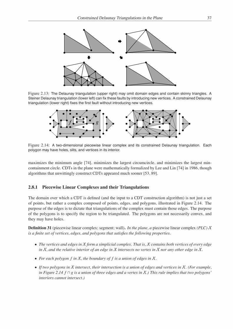
Constrained Delaunay Triangulations in the Plane 37
Figure 2.13: The Delaunay triangulation (upper right) may omit domain edges and contain skinny triangles. ASteiner Delaunay triangulation (lower left) can fix these faults by introducing new vertices. A constrained Delaunaytriangulation (lower right) fixes the first fault without introducing new vertices.
gf
Figure 2.14: A two-dimensional piecewise linear complex and its constrained Delaunay triangulation. Eachpolygon may have holes, slits, and vertices in its interior.
maximizes the minimum angle [74], minimizes the largest circumcircle, and minimizes the largest min-containment circle. CDTs in the plane were mathematically formalized by Lee and Lin [74] in 1986, thoughalgorithms that unwittingly construct CDTs appeared much sooner [53, 89].
2.8.1 Piecewise Linear Complexes and their Triangulations
The domain over which a CDT is defined (and the input to a CDT construction algorithm) is not just a setof points, but rather a complex composed of points, edges, and polygons, illustrated in Figure 2.14. Thepurpose of the edges is to dictate that triangulations of the complex must contain those edges. The purposeof the polygons is to specify the region to be triangulated. The polygons are not necessarily convex, andthey may have holes.
Definition 31 (piecewise linear complex; segment; wall). In the plane, a piecewise linear complex (PLC) Xis a finite set of vertices, edges, and polygons that satisfies the following properties.
• The vertices and edges inX form a simplicial complex. That is, X contains both vertices of every edgein X, and the relative interior of an edge in X intersects no vertex in X nor any other edge in X.
• For each polygon f in X, the boundary of f is a union of edges in X.
• If two polygons in X intersect, their intersection is a union of edges and vertices in X. (For example,in Figure 2.14 f ∩ g is a union of three edges and a vertex in X.) This rule implies that two polygons’interiors cannot intersect.)

38 Jonathan Richard Shewchuk
Following Ruppert [102], the edges in a PLC X are called segments to distinguish them from otheredges in a triangulation of X. The polygons in a PLC are called walls.
The underlying space of a PLCX, denoted |X|, is the union of its contents; that is, |X| ="
f∈X f . Usually,the underlying space is the domain to be triangulated.1
Every simplicial complex and every polyhedral complex is a PLC. But PLCs are more general, and notjust because they permit nonconvex polygons. As Figure 2.14 illustrates, segments and isolated verticescan float in a wall’s interior, constraining how the wall can be triangulated. One purpose of these floatingconstraints is to permit the application of boundary conditions at appropriate locations in a mesh of a PLC.
Whereas the faces of a simplex are defined in a way that depends solely on the simplex, and the faces ofa convex polyhedron are too, the faces of a wall are defined in a fundamentally different way that dependson both the wall and the PLC it is a part of. An edge of a wall might be a union of several segments in thePLC; these segments and their vertices are faces of the wall. A PLC may contain segments and edges thatlie in the relative interior of a wall; these are also considered to be faces of the wall, because they constrainhow the wall can be subdivided into triangles.
Definition 32 (face of a linear cell). The faces of a linear cell (polygon, edge, or vertex) f in a PLC X arethe linear cells in X that are subsets of f , including f itself.
A triangulation of X must cover every wall and include every segment.
Definition 33 (triangulation of a planar PLC). Let X be a PLC in the plane. A triangulation of X is asimplicial complex T such that
• X and T have the same vertices,
• T contains every edge in X (and perhaps additional edges), and
• |T | = |X|.
It is not difficult to see that a simplex can appear in a triangulation of X only if it respects X.
Definition 34 (respect). A simplex σ respects a PLC X if σ ⊆ |X| and for every f ∈ X that intersects σ,f ∩ σ is a union of faces of σ. (Usually, but not always, that union is one face of σ or σ itself.) In otherwords, f fully includes every face of σ whose relative interior intersects f .
Theorem 12. Every simple polygon has a triangulation. Every PLC in the plane has a triangulation too.
Proof: Let P be a simple polygon. If P is a triangle, it clearly has a triangulation. Otherwise, consider thefollowing procedure for triangulating P. Let ∠uvw be a corner of P having an interior angle less than 180.Two such corners are found by letting v be the lexicographically least or greatest vertex of P.
If the open edge uw lies strictly in P’s interior, then cutting uvw from P yields a polygon having oneedge fewer; triangulate it recursively. Otherwise, uvw contains at least one vertex of P besides u, v, andw, as illustrated in Figure 2.15. Among those vertices, let x be the vertex furthest from the line aff uw. Theopen edge vx must lie strictly in P’s interior, because if it intersected an edge of P, that edge would have avertex further from aff uw. Cutting P at vx produces two simple polygons, each with fewer edges than P;triangulate them recursively. In either case, the procedure produces a triangulation of P.
1If you take the vertices and edges of a planar PLC and discard the polygons, you have a simplicial complex with no triangles.This complex is called a planar straight line graph (PSLG). Most publications about CDTs take a PSLG as the input, and assumethat the CDT should cover the PSLG’s convex hull. PLCs are more expressive, as they can restrict the triangulation to a nonconvexregion of the plane.
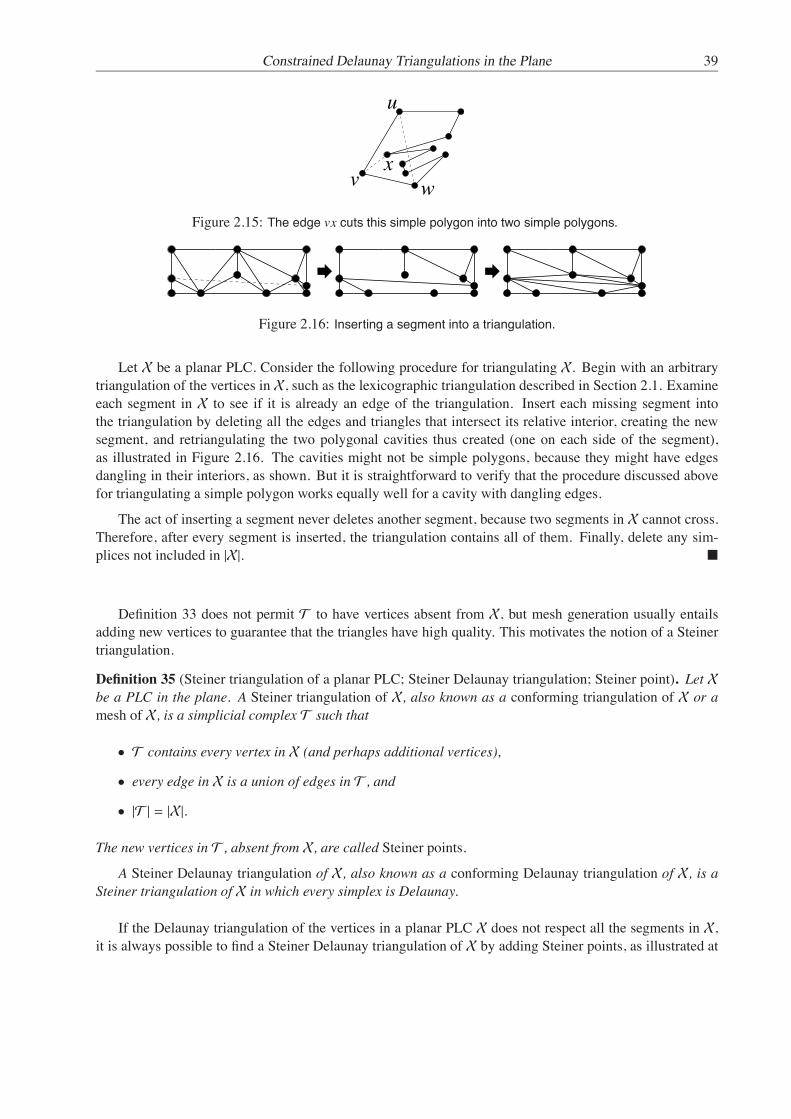
Constrained Delaunay Triangulations in the Plane 39
x
u
v wFigure 2.15: The edge vx cuts this simple polygon into two simple polygons.
Figure 2.16: Inserting a segment into a triangulation.
Let X be a planar PLC. Consider the following procedure for triangulating X. Begin with an arbitrarytriangulation of the vertices in X, such as the lexicographic triangulation described in Section 2.1. Examineeach segment in X to see if it is already an edge of the triangulation. Insert each missing segment intothe triangulation by deleting all the edges and triangles that intersect its relative interior, creating the newsegment, and retriangulating the two polygonal cavities thus created (one on each side of the segment),as illustrated in Figure 2.16. The cavities might not be simple polygons, because they might have edgesdangling in their interiors, as shown. But it is straightforward to verify that the procedure discussed abovefor triangulating a simple polygon works equally well for a cavity with dangling edges.
The act of inserting a segment never deletes another segment, because two segments in X cannot cross.Therefore, after every segment is inserted, the triangulation contains all of them. Finally, delete any sim-plices not included in |X|. "
Definition 33 does not permit T to have vertices absent from X, but mesh generation usually entailsadding new vertices to guarantee that the triangles have high quality. This motivates the notion of a Steinertriangulation.
Definition 35 (Steiner triangulation of a planar PLC; Steiner Delaunay triangulation; Steiner point). Let Xbe a PLC in the plane. A Steiner triangulation of X, also known as a conforming triangulation of X or amesh of X, is a simplicial complex T such that
• T contains every vertex in X (and perhaps additional vertices),
• every edge in X is a union of edges in T , and
• |T | = |X|.
The new vertices in T , absent from X, are called Steiner points.
A Steiner Delaunay triangulation of X, also known as a conforming Delaunay triangulation of X, is aSteiner triangulation of X in which every simplex is Delaunay.
If the Delaunay triangulation of the vertices in a planar PLC X does not respect all the segments in X,it is always possible to find a Steiner Delaunay triangulation of X by adding Steiner points, as illustrated at

40 Jonathan Richard Shewchuk
lower left in Figure 2.13. Unfortunately, the number of Steiner points might be large. The best algorithm todate, by Bishop [13], triangulates a PLC having m segments and n vertices with the addition of O(m2.5+mn)Steiner points. Edelsbrunner and Tan [49] exhibit a PLC requiring Θ(mn) Steiner points. Closing the gapbetween the O(m2.5 +mn) and Ω(mn) bounds remains an open problem. The large number of Steiner pointsthat some PLCs need motivates the constrained Delaunay triangulation, which needs none.
2.8.2 The Constrained Delaunay Triangulation
Constrained Delaunay triangulations (CDTs) offer a way to force a triangulation to respect the edges in aPLC without introducing new vertices, while maintaining some of the advantages of Delaunay triangula-tions. However, it is necessary to relax the requirement that all triangles be Delaunay. The terminology canbe confusing: whereas every Steiner Delaunay triangulation is a Delaunay triangulation (of some point set),constrained Delaunay triangulations generally are not.
Recall the Delaunay Lemma: a triangulation of a point set is Delaunay if and only if every edge is lo-cally Delaunay. Likewise, there is a Constrained Delaunay Lemma (Section 2.8.3) that offers the simplestdefinition of a CDT: a triangulation of a PLC is constrained Delaunay if and only if every edge is locallyDelaunay or a segment. Thus, a CDT differs from a Delaunay triangulation in three ways: it is not neces-sarily convex, it is required to contain the edges in a PLC, and those edges are exempted from being locallyDelaunay.
The defining characteristic of a CDT is that every triangle is constrained Delaunay, as defined below.
Definition 36 (visibility). Two points x and y are visible to each other if the line segment xy respects X;recall Definition 34. We also say that x and y can see each other. A linear cell in X that intersects therelative interior of xy but does not include xy is said to occlude the visibility between x and y.
Definition 37 (constrained Delaunay). In the context of a PLC X, a simplex σ is constrained Delaunay if itsatisfies the following three conditions.
• X contains σ’s vertices.
• σ respects X.
• There is a circumcircle of σ that encloses no vertex in X that is visible from a point in the relativeinterior of σ.
Figure 2.17 illustrates examples of a constrained Delaunay edge e and a constrained Delaunay triangleτ. Bold lines indicate PLC segments. Although e has no empty circumcircle, the depicted circumcircle ofe encloses no vertex that is visible from the relative interior of e. There are two vertices inside the circle,but both are hidden behind segments. Hence, e is constrained Delaunay. Similarly, the circumcircle of τencloses two vertices, but both are hidden from the interior of τ by segments, so τ is constrained Delaunay.
Definition 38 (constrained Delaunay triangulation). A constrained Delaunay triangulation (CDT) of a PLCX is a triangulation of X in which every triangle is constrained Delaunay.
Figure 2.18 illustrates a PLC, a Delaunay triangulation of its vertices, and a constrained Delaunay tri-angulation of the PLC. In the CDT, every triangle is constrained Delaunay, every edge that is not a PLCsegment is constrained Delaunay, and every vertex is trivially constrained Delaunay.

Constrained Delaunay Triangulations in the Plane 41
τe
Figure 2.17: The edge e and triangle τ are constrained Delaunay. Bold lines represent segments.
(a) (b) (c)
Figure 2.18: (a) A piecewise linear complex. (b) The Delaunay triangulation of its vertices. (c) Its constrainedDelaunay triangulation.
CDTs and Steiner Delaunay triangulations are two different ways to force a triangulation to conformto the boundary of a geometric domain. CDTs partly sacrifice the Delaunay property for the benefit ofrequiring no new vertices. For mesh generation, new vertices are usually needed anyway to obtain goodtriangles, so many Delaunay meshing algorithms use Steiner Delaunay triangulations. But some algorithmsuse a hybrid of CDTs and Steiner Delaunay triangulations because it helps to reduce the number of newvertices. A Steiner CDT or conforming CDT of X is a Steiner triangulation of X in which every triangle isconstrained Delaunay.
2.8.3 Properties of the Constrained Delaunay Triangulation
For every property of Delaunay triangulations discussed in this chapter, there is an analogous property ofconstrained Delaunay triangulations. This section summarizes them. Proofs are omitted, but each of themis a straightforward extension of the corresponding proof for Delaunay triangulations.
The Delaunay Lemma generalizes to CDTs, and provides a useful alternative definition: a triangulationof a PLC X is a CDT if and only if every one of its edges is locally Delaunay or a segment in X.
Theorem 13 (Constrained Delaunay Lemma). Let T be a triangulation of a PLC X. The following threestatements are equivalent.
• Every triangle in T is constrained Delaunay (i.e. T is constrained Delaunay).
• Every edge in T not in X is constrained Delaunay.

42 Jonathan Richard Shewchuk
• Every edge in T not in X is locally Delaunay. "
One way to construct a constrained Delaunay triangulation of a PLC X is to begin with any triangulationof X. Apply the flip algorithm, modified so that it never flips a segment: repeatedly choose any edge ofthe triangulation that is not in X and not locally Delaunay, and flip it. When no such edge survives, theDelaunay Lemma tells us that the triangulation is constrained Delaunay.
Theorem 14. Given a triangulation of a PLC having n vertices, the modified flip algorithm (which neverflips a PLC segment) terminates after O(n2) edge flips, yielding a constrained Delaunay triangulation. "
Corollary 15. Every PLC has a constrained Delaunay triangulation. "
The CDT has the same optimality properties as the Delaunay triangulation, except that the optimality iswith respect to a smaller set of triangulations—those that include the PLC’s edges.
Theorem 16. Among all the triangulations of a PLC, every constrained Delaunay triangulation maximizesthe minimum angle in the triangulation, minimizes the largest circumcircle, and minimizes the largest min-containment circle. "
A sufficient but not necessary condition for the CDT to be unique is that no four vertices are cocircular.
Theorem 17. If no four vertices in a PLC lie on a common circle, then the PLC has one unique constrainedDelaunay triangulation. "

Chapter 3
Algorithms for Constructing DelaunayTriangulations
The first published Delaunay triangulation algorithm I know of appears in a 1967 paper by J. DesmondBernal and John Finney [12]. Bernal was a father of structural biology who discovered the structure ofgraphite and was awarded a Stalin Peace Prize. Finney, Bernal’s last Ph.D. student, implemented a programthat produces a three-dimensional Voronoi diagram and used it to characterize the structures of liquids,amorphous metal alloys, protein molecules, and random packings. Finney’s is the brute force algorithm:test every possible tetrahedron (every combination of four vertices) to see if its circumsphere is empty,taking O(n5) time—or more generally, O(nd+2) time for d-dimensional Delaunay triangulations.
Besides this brute force algorithm and the flip algorithm, there are three classic types of algorithm forconstructing Delaunay triangulations.
Gift-wrapping—also called graph traversal, pivoting, and incremental search—is an obvious algorithmthat is rediscovered frequently [53, 26, 79, 121, 123]. Gift-wrapping algorithms construct Delaunay trianglesone at a time, using the previously computed triangles as a seed on which new triangles crystallize. They areclosely related to advancing front methods for mesh generation. Gift-wrapping generalizes easily to CDTsand to higher dimensions, and it is easy to implement, but it is difficult to make fast. Section 3.8 describesa basic gift-wrapping algorithm that triangulates n points in the plane in O(n2) worst-case time, or a PLCin the plane with n vertices and m segments in O(n2m) time. The bottleneck of gift-wrapping is identifyingnew triangles, so the fastest gift-wrapping algorithms are differentiated by sweep orderings for constructingthe triangles [108, 51] or sophisticated vertex search strategies [47, 120].
In the decision-tree model of computation, sets of n points in the plane sometimes require Ω(n log n)time to triangulate. The first Delaunay triangulation algorithm to run in optimalO(n log n) time was the 1975divide-and-conquer algorithm of Shamos and Hoey [111], subsequently simplified by Lee and Schachter [75]and Guibas and Stolfi [60] and sped up by Dwyer [46]. The divide-and-conquer algorithm partitions a set ofpoints into two halves separated by a line, recursively computes the Delaunay triangulation of each subset,and merges the two triangulations into one. This algorithm remains the fastest planar Delaunay triangulatorin practice [112], and the reader interested in implementing it is urged to read the guide by Guibas andStolfi [60], which includes detailed pseudocode. However, the divide-and-conquer strategy is not fast inthree dimensions.
Incremental insertion algorithms insert vertices into a Delaunay triangulation one at a time, alwaysrestoring the Delaunay property to the triangulation before inserting another vertex. Some incremental in-sertion algorithms run in worst-case optimal time. The fastest three-dimensional Delaunay triangulators in
43

44 Jonathan Richard Shewchuk
practice are in this class. Moreover, the difference between a Delaunay triangulation algorithm and a mod-ern Delaunay mesh generator is that the former is given all the vertices at the outset, whereas the latter usesthe triangulation to decide where to place additional vertices, making incremental insertion obligatory. Sec-tions 3.3–3.5 study incremental insertion, and Section 5.4 introduces a more sophisticated vertex orderingmethod called a biased randomized insertion order that speeds up incremental insertion for large points sets.
All three types of algorithm extend to constrained Delaunay triangulations. There are a divide-and-conquer algorithm [34] and a gift-wrapping algorithm [109] that both run in worst-case optimal O(n log n)time, but because they are complicated, these algorithms are rarely implemented.
The most commonly used CDT construction method in practice is incremental insertion: first constructa Delaunay triangulation of the PLC’s vertices, then insert the PLC’s segments one by one. The algorithmscommonly used to perform segment insertion in practice are slow, but a specialized incremental algorithmdescribed in Section 3.9 runs in expected O(n log n+ n log2 m) time. Realistic PLCs have few segments longenough to cross many edges, and it is typical to observe O(n log n) running time in practice.
3.1 The Orientation and Incircle Predicates
Most geometric algorithms perform a mix of combinatorial and numerical computations. The numericalcomputations are usually packaged as geometric primitives of two types: geometric constructors that createnew entities, such as the point where two specified lines intersect, and geometric predicates that determinerelationships among entities, such as whether or not two lines intersect at all. Many Delaunay triangulationalgorithms require just two predicates, called the orientation and incircle tests.
The most used predicate in computational geometry is the orientation test. Let a, b, and c be three pointsin the plane. Consider a function Orient2D(a, b, c) that returns a positive value if the points a, b, and care arranged in counterclockwise order, a negative value if the points are in clockwise order, and zero ifthe points are collinear. Another interpretation, important for many geometric algorithms, is that Orient2Dreturns a positive value if a lies to the left of the directed line bc. The orientation test can be implementedas a matrix determinant that computes the signed area of the parallelogram determined by the vectors a − cand b − c,
Orient2D(a, b, c) =
%
%
%
%
%
%
%
%
%
ax ay 1bx by 1cx cy 1
%
%
%
%
%
%
%
%
%
(3.1)
=
%
%
%
%
%
%
ax − cx ay − cybx − cx by − cy
%
%
%
%
%
%
. (3.2)
These expressions extend to higher dimensions by adding rows and columns for additional points andcoordinate axes. Given four points a, b, c, and d in E3, define Orient3D(a, b, c, d) to be the signed volumeof the parallelepiped determined by the vectors a − d, b − d, and c − d. It is positive if the points occur inthe orientation illustrated in Figure 3.1, negative if they occur in the mirror-image orientation, and zero ifthe four points are coplanar. You can apply a right-hand rule: orient your right hand with fingers curled tofollow the circular sequence bcd. If your thumb points toward a, Orient3D is positive.
Orient3D(a, b, c, d) =
%
%
%
%
%
%
%
%
%
%
%
ax ay az 1bx by bz 1cx cy cz 1dx dy dz 1
%
%
%
%
%
%
%
%
%
%
%
=
%
%
%
%
%
%
%
%
%
ax − dx ay − dy az − dzbx − dx by − dy bz − dzcx − dx cy − dy cz − dz
%
%
%
%
%
%
%
%
%
.

The Orientation and Incircle Predicates 45
c
c d
a ba b
Figure 3.1: A triangle and a tetrahedron, both having positive orientation.
Most planar Delaunay triangulation algorithms use a predicate InCircle(a, b, c, d) that returns a positivevalue if d lies inside the unique (and possibly degenerate) circle through a, b, and c, assuming that the latterthree points occur in counterclockwise order around the circle. InCircle returns zero if and only if all fourpoints lie on a common circle or line. InCircle is derived from Orient3D and Lemma 1, which showsthat testing whether a point is inside a circle is equivalent to an orientation test on the points lifted by theparabolic lifting map.
InCircle(a, b, c, d) =
%
%
%
%
%
%
%
%
%
%
%
%
ax ay a2x + a2
y 1bx by b2
x + b2y 1
cx cy c2x + c2
y 1dx dy d2
x + d2y 1
%
%
%
%
%
%
%
%
%
%
%
%
(3.3)
=
%
%
%
%
%
%
%
%
%
ax − dx ay − dy (ax − dx)2 + (ay − dy)2
bx − dx by − dy (bx − dx)2 + (by − dy)2
cx − dx cy − dy (cx − dx)2 + (cy − dy)2
%
%
%
%
%
%
%
%
%
. (3.4)
These expressions also extend easily to higher dimensions. Let a, b, c, d, and e be five points in E3,with the first four ordered so that Orient3D(a, b, c, d) is nonnegative. The function InSphere(a, b, c, d, e) ispositive if e lies inside the sphere passing through a, b, c, and d; negative if e lies outside the sphere; andzero if all five points are cospherical or coplanar.
InSphere(a, b, c, d, e) =
%
%
%
%
%
%
%
%
%
%
%
%
%
%
%
ax ay az a2x + a2
y + a2z 1
bx by bz b2x + b2
y + b2z 1
cx cy cz c2x + c2
y + c2z 1
dx dy dz d2x + d2
y + d2z 1
ex ey ez e2x + e2
y + e2z 1
%
%
%
%
%
%
%
%
%
%
%
%
%
%
%
=
%
%
%
%
%
%
%
%
%
%
%
ax − ex ay − ey az − ez (ax − ex)2 + (ay − ey)2 + (az − ez)2
bx − ex by − ey bz − ez (bx − ex)2 + (by − ey)2 + (bz − ez)2
cx − ex cy − ey cz − ez (cx − ex)2 + (cy − ey)2 + (cz − ez)2
dx − ex dy − ey dz − ez (dx − ex)2 + (dy − ey)2 + (dz − ez)2
%
%
%
%
%
%
%
%
%
%
%
.
Orient2D, Orient3D, InCircle, and InSphere have the symmetry property that interchanging any two oftheir parameters reverses their sign. If the points a, b, c occur in clockwise order, InCircle behaves as if thecircle’s outside were its inside. Likewise, if Orient3D(a, b, c, d) is negative, the sign returned by InSphereis reversed.
Expressions (3.1) and (3.2) can be shown to be equivalent by simple algebraic transformations, as canExpressions (3.3) and (3.4) with a little more effort. Expressions (3.2) and (3.4) should be strongly preferred

46 Jonathan Richard Shewchuk
Procedure PurposeAddTriangle(u, v,w) Add a positively oriented triangle uvwDeleteTriangle(u, v,w) Delete a positively oriented triangle uvwAdjacent(u, v) Return a vertex w such that uvw is a positively oriented triangleAdjacentOne(u) Return vertices v, w such that uvw is a positively oriented triangle
Figure 3.2: An interface for a triangulation data structure.
over Expressions (3.1) and (3.3) for fixed precision floating-point computation, because they lose far lessaccuracy to roundoff error. Ideally, some form of exact arithmetic should be used to perform these tests, orthe triangulation algorithms cannot be guaranteed to work correctly.
3.2 A Dictionary Data Structure for Triangulations
Two data structures are commonly used to implement triangulation algorithms: edge-based data structures,of which the best known is the doubly connected edge list [86], and triangle-based data structures. Whatthese two data structures have in common is that records represent edges or triangles, and the records storepointers that point at neighboring edges or triangles. Many implementations of triangulation algorithms readand change these pointers directly; experience shows that these implementations are difficult to code anddebug.
Here, I advocate an interface that does not expose pointers to the triangulation algorithms that use thedata structure. Triangulation algorithms access the triangulation in a natural way, by adding or deletingtriangles specified by their vertices. It is wholly the responsibility of the triangulation storage library todetermine triangle adjacencies, and to correctly maintain any pointers it uses internally. This policy, whichoriginates with Blelloch et al. [17, 16], improves programmer productivity and simplifies debugging.
The interface appears in Figure 3.2. Two procedures, AddTriangle and DeleteTriangle, create anddelete triangles by specifying the vertices of a triangle, ordered so that all the triangles stored in the datastructure have positive orientation. The data structure enforces the invariant that only two triangles mayadjoin an edge, and only one on each side of the edge. Therefore, if the data structure contains a positivelyoriented triangle uvw and an application calls AddTriangle(u, v, x), the triangle uvx is rejected and thedata structure does not change.
At least two query operations are supported. The procedure Adjacent(u, v) returns a vertex w if thetriangulation includes a positively oriented triangle uvw, or the empty set otherwise. Adjacent(u, v) andAdjacent(v, u) return different triangles, on opposite sides of the edge uv. The procedure AdjacentOne(u)identifies an arbitrary triangle having vertex u, or returns the empty set if no such triangle exists.
A fast way to implement Adjacent efficiently is to store each triangle uvw three times in a hash table,keyed on the directed edges uv, vw, and wu. A hash table can store triangles and query edges in expectedconstant time. For a more compact representation that is still reasonably fast, see Blandford, Blelloch,Clemens, and Kadow [16].
Unfortunately, it takes substantial additional memory to guarantee that the AdjacentOne query will runfast. Many algorithms for Delaunay triangulation and meshing can be implemented without it, so I recom-mend using AdjacentOne as little as possible, and settling for a slow but memory-efficient implementation,perhaps even searching the entire hash table. A good compromise implementation is to maintain an array

Inserting a Vertex into a Delaunay Triangulation 47
Figure 3.3: The Bowyer–Watson algorithm in the plane. At left, a Delaunay triangulation and a new vertex toinsert. At center, every triangle whose circumcircle encloses the new vertex is shaded. These triangles are nolonger Delaunay. At right, the shaded triangles disappear, replaced by new triangles that connect the new vertexto the edges of the cavity.
that stores, for each vertex u, a vertex v such that the most recently added triangle adjoining u also had vfor a vertex. When AdjacentOne(u) is invoked, it looks up the edges uv and vu in the hash table to findan adjoining triangle in expected constant time. The problem with this implementation is that the triangleshaving edge uv may have been subsequently deleted, in which case a triangle adjoining u must be foundsome other way (e.g. searching the entire hash table). However, observe that this catastrophe will not occurif every triangle deletion is followed by triangle creations that cover all the same vertices—which is true ofmost of the algorithms discussed in this book.
The interface and data structure extend easily to permit the storage of edges that are not part of anytriangle. For example, an edge uv that is not an edge of any triangle can be represented by storing uvgkeyed on the directed edge uv, where g is a special entity called the ghost vertex.
3.3 Inserting a Vertex into a Delaunay Triangulation
Lawson [73] invented the first algorithm for inserting a vertex into a Delaunay triangulation and restoringthe Delaunay property, but it works only in the plane. A slightly faster algorithm that works in any dimen-sionality was discovered independently by Bowyer [20], Hermeline [62, 63], and Watson [128]. Bowyer andWatson simultaneously submitted it to Computer Journal and found their articles published side by side.
Consider inserting a new vertex v into a Delaunay triangulation. If a triangle’s circumcircle encloses v,that triangle is no longer Delaunay, so it must be deleted. This suggests the Bowyer–Watson algorithm.
• Find one triangle whose circumcircle encloses v.
• Find all the others (in time linear in their number) by a depth-first search in the triangulation.
• Delete them all, evacuating a polyhedral cavity, which is shaded in Figure 3.3.
• For each edge of this cavity, create a new triangle joining it with v, as illustrated.
The first step is called point location. Most Delaunay mesh generation algorithms generate new verticesinside the circumcircles of badly shaped or oversized triangles, in which case point location is free. However,point location is not free for the domain vertices provided as input to the mesh generator. Locating thesepoints in the triangulation is sometimes the most costly and complicated part of the incremental insertionalgorithm. Incremental insertion is really a class of Delaunay triangulation algorithms, differentiated by theirpoint location methods. Clarkson and Shor [39] describe a point location method that helps a randomized
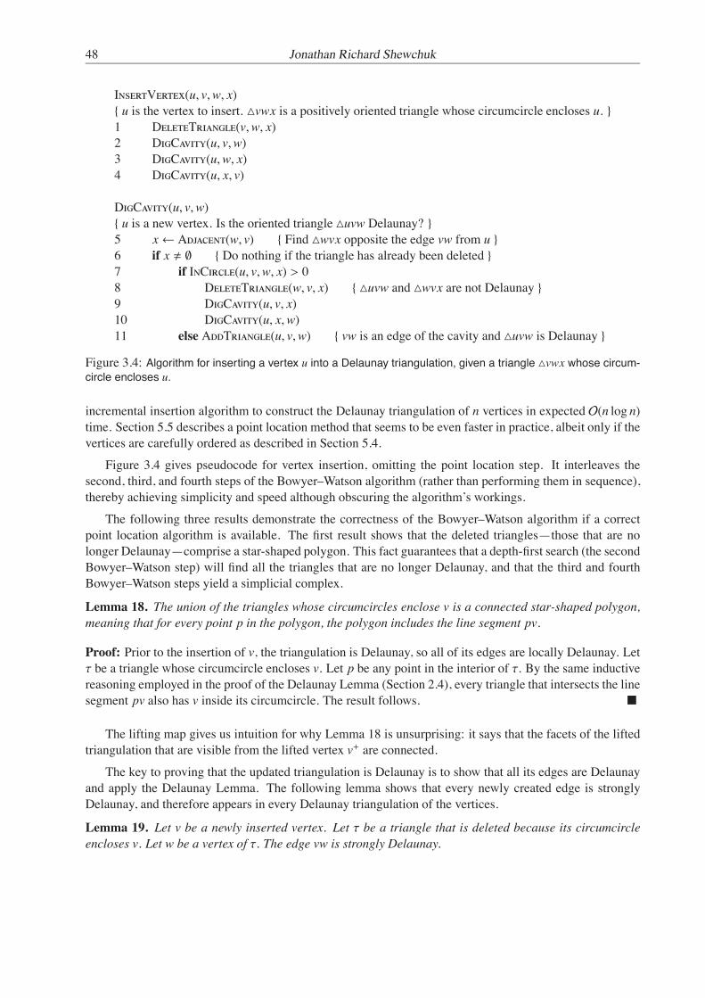
48 Jonathan Richard Shewchuk
InsertVertex(u, v,w, x) u is the vertex to insert. vwx is a positively oriented triangle whose circumcircle encloses u. 1 DeleteTriangle(v,w, x)2 DigCavity(u, v,w)3 DigCavity(u,w, x)4 DigCavity(u, x, v)
DigCavity(u, v,w) u is a new vertex. Is the oriented triangle uvw Delaunay? 5 x← Adjacent(w, v) Find wvx opposite the edge vw from u 6 if x ! ∅ Do nothing if the triangle has already been deleted 7 if InCircle(u, v,w, x) > 08 DeleteTriangle(w, v, x) uvw and wvx are not Delaunay 9 DigCavity(u, v, x)10 DigCavity(u, x,w)11 else AddTriangle(u, v,w) vw is an edge of the cavity and uvw is Delaunay
Figure 3.4: Algorithm for inserting a vertex u into a Delaunay triangulation, given a triangle vwx whose circum-circle encloses u.
incremental insertion algorithm to construct the Delaunay triangulation of n vertices in expected O(n log n)time. Section 5.5 describes a point location method that seems to be even faster in practice, albeit only if thevertices are carefully ordered as described in Section 5.4.
Figure 3.4 gives pseudocode for vertex insertion, omitting the point location step. It interleaves thesecond, third, and fourth steps of the Bowyer–Watson algorithm (rather than performing them in sequence),thereby achieving simplicity and speed although obscuring the algorithm’s workings.
The following three results demonstrate the correctness of the Bowyer–Watson algorithm if a correctpoint location algorithm is available. The first result shows that the deleted triangles—those that are nolonger Delaunay—comprise a star-shaped polygon. This fact guarantees that a depth-first search (the secondBowyer–Watson step) will find all the triangles that are no longer Delaunay, and that the third and fourthBowyer–Watson steps yield a simplicial complex.
Lemma 18. The union of the triangles whose circumcircles enclose v is a connected star-shaped polygon,meaning that for every point p in the polygon, the polygon includes the line segment pv.
Proof: Prior to the insertion of v, the triangulation is Delaunay, so all of its edges are locally Delaunay. Letτ be a triangle whose circumcircle encloses v. Let p be any point in the interior of τ. By the same inductivereasoning employed in the proof of the Delaunay Lemma (Section 2.4), every triangle that intersects the linesegment pv also has v inside its circumcircle. The result follows. "
The lifting map gives us intuition for why Lemma 18 is unsurprising: it says that the facets of the liftedtriangulation that are visible from the lifted vertex v+ are connected.
The key to proving that the updated triangulation is Delaunay is to show that all its edges are Delaunayand apply the Delaunay Lemma. The following lemma shows that every newly created edge is stronglyDelaunay, and therefore appears in every Delaunay triangulation of the vertices.
Lemma 19. Let v be a newly inserted vertex. Let τ be a triangle that is deleted because its circumcircleencloses v. Let w be a vertex of τ. The edge vw is strongly Delaunay.

Inserting a Vertex Outside a Delaunay Triangulation 49
τ
v
wC
Figure 3.5: Because τ was Delaunay before v was inserted, vw is strongly Delaunay.
Figure 3.6: Inserting a vertex outside the triangulation. The open circle is the ghost vertex. The circular arrowindicates two ghost edges that are really the same edge. Three ghost triangles and three solid triangles (shaded)are deleted and replaced with two new ghost triangles and six new solid triangles.
Proof: See Figure 3.5. The circumcircle of τ encloses no vertex but v. Let C be the circle that is tangent toτ’s circumcircle at w and passes through v. C demonstrates that vw is strongly Delaunay. "
Theorem 20. A triangulation produced by applying the Bowyer–Watson algorithm to a Delaunay triangu-lation is Delaunay.
Proof: It follows from Lemma 18 that the update produces a triangulation of the point set augmented withthe new point. All the surviving old triangles are Delaunay; otherwise they would have been deleted. Itfollows that their edges are Delaunay too. By Lemma 19, all of the newly created edges are Delaunay aswell. By the Delaunay Lemma, the new triangulation is Delaunay. "
3.4 Inserting a Vertex Outside a Delaunay Triangulation
The Bowyer–Watson algorithm works only if the newly inserted vertex lies in the triangulation. However,there is an elegant way to represent a triangulation so that the algorithm, with almost no changes, can inserta vertex outside the triangulation equally well. Imagine that every edge on the boundary of the triangulationadjoins a ghost triangle, as illustrated in Figure 3.6. The third vertex of every ghost triangle is the ghostvertex, a vertex “at infinity” shared by every ghost triangle. Every ghost triangle has two ghost edges thatadjoin the ghost vertex. A triangle that is not a ghost is called a solid triangle.
The ghost triangles are explicitly stored in the triangulation data structure. They are not merely cosmetic;they make it possible for the Bowyer–Watson algorithm to efficiently traverse the triangulation boundary,and thus they are essential to obtaining an incremental insertion algorithm with optimal running time.

50 Jonathan Richard Shewchuk
g
Figure 3.7: The ghost triangle uvg is deleted if a new vertex is inserted in the shaded open halfplane (as atcenter) or on uv (as at right). The union of the open halfplane and uv is the outer halfplane of uvg.
Consider an edge uv on the boundary of a triangulation, directed clockwise around the boundary. Definea positively oriented ghost triangle uvg, where g is the ghost vertex. Like any other triangle, uvg hasa circumcircle—albeit a degenerate one—and must be deleted if a new vertex is inserted “inside” it. Thedefinition of “circumcircle” is a bit tricky, though. The circumcircle degenerates to the line aff uv, whichdivides the plane into two open halfplanes.
There are two cases in which the ghost triangle uvg must be deleted (i.e. uv is no longer a boundaryedge of the triangulation), both illustrated in Figure 3.7: if a vertex is inserted in the open halfplane on theother side of aff uv from the triangulation, or if a vertex is inserted on the open edge uv. Call the union ofthese two regions the outer halfplane of uv. It is neither an open nor closed halfplane, but something inbetween. It is the set of points enclosed by the circumcircle of uvg in the limit as g moves away from thetriangulation.
A new vertex inserted outside the triangulation causes at least one ghost triangle to be deleted, andperhaps some solid (non-ghost) triangles as well. Two new boundary edges, two new ghost triangles, and anarbitrary number of solid triangles are created, as illustrated in Figure 3.6.
Ghost triangles have an intuitive interpretation in terms of the lifting map. Imagine that in E3, the solidtriangles are lifted to the paraboloid, and the ghost triangles and ghost edges are vertical—parallel to thez-axis. By magic, the ghost vertex is interpreted as being directly above every other vertex at an infiniteheight. The faces of the convex hull of this three-dimensional point set, including the magic ghost vertex,are in one-to-one correspondence with the faces and ghost faces of the Delaunay triangulation.
A popular alternative to ghost triangles is to enclose the input vertices in a giant triangular boundingbox, illustrated in Figure 3.8. After all the vertices have been inserted, every triangle having a boundingbox vertex is deleted. The difficulty with this approach is that the bounding box vertices may leave concavedivots in the triangulation if they are too close, and it is not easy to determine how far away they needto be. One solution to this problem is to compute a weighted Delaunay triangulation, assigning the threebounding box vertices weights of negative infinity. These three infinite weights must be incomparable—say,∞, 2∞, and 22∞—so that InCircle tests involving two of the bounding box vertices operate consistently.This approach seems to run more slowly (perhaps by 10%) than the ghost triangle implementation. Anothersolution is to fill the divots with the segment insertion algorithm described in Section 3.9.
3.5 The Running Time of Vertex Insertion
How expensive is vertex insertion, leaving out the cost of point location? This section considers two cases:the worst case, and the expected case when vertices are inserted in random order. The latter case is a partof an incremental insertion algorithm that computes the Delaunay triangulation of n vertices in expectedO(n log n) time, and it also introduces an elegant algorithm analysis technique called backward analysis.

The Running Time of Vertex Insertion 51
Figure 3.8: Enclosing the vertices in a large triangular bounding box.
Figure 3.9: Each vertex insertion can delete Θ(n) triangles and create Θ(n) others.
Figure 3.9 illustrates the worst case. A single vertex insertion can delete Θ(n) triangles and create Θ(n)others, taking Θ(n) time. Moreover, this dismal performance can be repeated for Θ(n) successive vertexinsertions. Therefore, the incremental insertion algorithm for constructing a Delaunay triangulation takesΘ(n2) time if the vertices and their insertion order are chosen badly. The grid arrangement and vertexordering in the figure are common in practice.
Fortunately, there are better ways to order the vertex insertion operations. The randomized incrementalinsertion algorithm inserts the vertices in random order, with each permutation of the vertices being equallylikely. Surprisingly, the expected number of triangles created by each successive vertex insertion operationis less than six, as Theorem 21 below shows. The catch is that all the vertices must be known in advance, sothat a random permutation can be computed. The randomized algorithm is excellent for creating an initialtriangulation of the vertices of a domain, but its analysis does not apply to the vertices that are subsequentlygenerated during mesh generation, because their order cannot be randomized. Nevertheless, the theoremprovides intuition for why constant-time vertex insertion is so commonly observed in mesh generation.
Theorem 21. Let V be a set of n vertices in the plane. Let ⟨v1, v2, . . . , vn⟩ be a permutation of V chosenuniformly at random from the set of all such permutations. For i ∈ [0, n], letTi be the Delaunay triangulationconstructed by inserting the first i vertices in order. When vi is inserted into Ti−1 to create Ti, the expectednumber of new triangles (including ghost triangles) created is less than six. An expected total of O(n)triangles are created and deleted during the n vertex insertions that construct Tn.
This theorem is most easily proved with backward analysis, a remarkable analysis technique that Sei-del [110] summarizes thus: “Analyze an algorithm as if it was running backwards in time, from output toinput.” Imagine that instead of inserting a randomly chosen vertex into Ti−1, you are deleting a randomlychosen vertex from Ti. Because a random permutation written backward is still a random permutation, eachvertex in Ti is deleted with equal probability.

52 Jonathan Richard Shewchuk
Proof of Theorem 21: For every vertex v of Ti, the number of triangles adjoining v, including ghosttriangles, is equal to the degree of v, counting one ghost edge if v is on the boundary of the triangulation.When vi is inserted into Ti−1 to construct Ti, every new triangle created has vi for a vertex. Therefore, theexpected number of new triangles created is equal to the expected degree of vi.
There is one technical difficulty: if four vertices of Ti lie on a common empty circle, then Ti dependson the order in which the vertices are inserted. Thus, let S i be the Delaunay subdivision of v1, v2, . . . , vi,wherein triangles in Ti sharing a common circumcircle are merged into a polygon. Recall from Section 2.2that S i contains the strongly Delaunay edges of Ti and no others, and is therefore unique. By Lemma 19,every edge adjoining vi in Ti is strongly Delaunay, so the degree of vi in Ti is equal to the degree of vi in S i.
Because the permutation is chosen uniformly at random, each vertex of S i is equally likely to be vi. Theexpected degree of a randomly chosen vertex in S i (or any planar graph) is less than six, by the followingreasoning.
Let i + 1, e, and f denote the number of vertices, edges, and triangles of Ti, respectively, with the ghostvertex, ghost edges, and ghost triangles included. By Euler’s formula, i + 1 − e + f = 2. Each triangle hasthree edges, and each edge is shared by two triangles, so 2e = 3 f . Eliminating f from Euler’s formula givese = 3i − 3. Each edge has two vertices, so the total number of edge-vertex incidences is 6i − 6, and theaverage degree of a non-ghost vertex in Ti is less than 6 − 6/i. The average degree of a non-ghost vertex inS i cannot be greater.
Each vertex insertion creates, in expectation, fewer than six new triangles, so the expected total numberof triangles created during the n vertex insertions is in O(n). A triangle cannot be deleted unless it is createdfirst, so the expected total number of triangles deleted is also in O(n). "
Theorem 21 bounds not only the number of structural changes, but also the running time of the depth-first search in the Bowyer–Watson algorithm. This search visits all the triangles that are deleted and all thetriangles that share an edge with a deleted triangle. Depth-first search takes time linear in the number ofvisited triangles, and therefore linear in the number of deleted triangles.
It follows that the expected running time of the randomized incremental insertion algorithm, excludingpoint location, is in O(n). We shall see that point location is the dominant cost of the algorithm.
A general fact about randomized algorithms is that there is a chance that they will run much, much moreslowly than their expected running time, but the probability of that is exceedingly small. If the incrementalinsertion algorithm gets unlucky and endures a slow vertex insertion like those depicted in Figure 3.9, other,faster vertex insertions will probably make up for it. The probability that many such slow vertex insertionswill occur in one run is tiny, but it can happen.
The argument in the proof of Theorem 21, which is the first known use of backward analysis in computa-tional geometry, originates in a paper by Chew [36]. Chew’s paper describes an algorithm for computing theDelaunay triangulation of a convex polygon, or deleting a vertex from a Delaunay triangulation, in expectedlinear time. Backward analysis was popularized by a charming paper by Seidel [110].
3.6 Inserting a Vertex into a Constrained Delaunay Triangulation
To “insert a vertex into a CDT” is to take as input the CDT of some PLC X and a new vertex v to insert,and produce the CDT of X ∪ v. An implementation might also support the insertion of a vertex v on a

The Gift-Wrapping Step 53
τdeletion
insertion
v
T’T
G
τ
Figure 3.10: Inserting or deleting a vertex v in a CDT. Bold edges are segments. The shaded polygon is the unionof the deleted/created triangles. Simplices not intersecting the interior of the shaded polygon are constrainedDelaunay before and after. When v is inserted, depth-first search on the graph G identifies the deleted triangles.Observe that although v lies inside τ’s circumcircle, v’s insertion does not delete τ because G does not connect τto any deleted triangle.
segment s ∈ X, in which case the algorithm subdivides s into two subsegments s1 and s2 having vertex v,and produces the CDT of X ∪ v, s1, s2 \ s.
With a small change, the Bowyer–Watson algorithm can insert a vertex v into a CDT, as Figure 3.10illustrates. The change, of course, is that the algorithm deletes the triangles that are no longer constrainedDelaunay. Fortunately, it is possible to enumerate those triangles without performing expensive visibilitytests. To accomplish that, the first step—point location—finds the triangle that contains v. There may betwo such triangles, if v lies on a triangulation edge. The second step—the depth-first search that identifiestriangles that are no longer constrained Delaunay—should never walk across a segment. As Figure 3.10shows, this restriction suffices to ensure that only triangles whose interiors are visible from v will be deleted.If v lies on a segment in X, depth-first searches must be run from both of the two adjoining triangles. Thethird and fourth steps of the Bowyer–Watson algorithm do not change. In a straightforward extension ofthe proofs in Section 3.3, one can show that the depth-first search finds all the triangles that are no longerconstrained Delaunay, the cavity is always star-shaped, and the algorithm works correctly.
3.7 The Gift-Wrapping Step
Gift-wrapping algorithms rely on a simple procedure that constructs a triangle adjoining a specified edge.Let e = uw be an oriented edge. The front of e is the open halfplane to the left of uw, and a positivelyoriented triangle uwv is said to be in front of e. The back of e is the open halfplane to the right of uw, anda positively oriented triangle wuv is said to be behind e.
During the execution of a gift-wrapping algorithm, an oriented edge constructed by the algorithm is saidto be unfinished if the algorithm has not yet identified the triangle in front of the edge. A gift-wrapping stepfinishes the edge by constructing that triangle, or by determining that there is no such triangle because theedge is on the boundary of the domain.
A edge e has an infinite number of circumcircles, any one of which can be continuously deformedinto any other such that every intermediate circle is also a circumcircle of e. Imagine beginning with acircumcircle that encloses no vertex in front of e, then deforming it so it expands in front of e and shrinksbehind e, always remaining a circumcircle of e, as illustrated in Figure 3.11. As the circumcircle deforms,its center always lies on e’s bisector.

54 Jonathan Richard Shewchuk
e
v
Figure 3.11: An empty circumcircle of e, expanding in search of a vertex v.
Finish(e,V,K) e is an oriented edge. V is the set of vertices in a PLC X. K is the set of segments in X. Finish returns a triangle that finishes e, or ∅ if none exists. 1 τ← ∅2 p← an arbitrary point in the relative interior of e (e.g. its midpoint)3 for each vertex v ∈ V4 if v is in front of e and (τ = ∅ or the circumcircle of τ encloses v)5 if no segment s ∈ K occludes the visibility between v and p6 τ← conv(e ∪ v)7 return τ
Figure 3.12: Algorithm to gift-wrap one constrained Delaunay triangle. For an ordinary Delaunay triangulation,omit Line 5.
Eventually, the expanding portion of the circumcircle might touch a vertex v that is visible from therelative interior of e, in which case the gift-wrapping step constructs τ = conv(e ∪ v), thereby finishinge. Lemma 22 below shows that τ is constrained Delaunay if e is constrained Delaunay or a segment.Alternatively, the expanding portion of the circumcircle might never touch a vertex, in which case e ison the boundary of the convex hull of the vertices.
Although the expanding circumcircle gives the right intuition for which vertex is chosen, the algorithmthat implements a gift-wrapping step works the opposite way, by shrinking the front of the circumcircle: itscans through the vertices in front of e and remembers which vertex, so far, minimizes the portion of thecircumcircle in front of e.
Figure 3.12 gives pseudocode for the gift-wrapping step. One gift-wrapping step takes O(n) time for aDelaunay triangulation, or O(nm) time for a CDT, where n = |V | is the number of vertices and m = |K| is thenumber of segments. Line 5 of the pseudocode accounts for the factor of m.
Lemma 22. If the edge e is constrained Delaunay or a segment, the algorithm Finish returns a constrainedDelaunay triangle τ.
Proof. There is a total ordering of the set of all e’s circumcircles such that, if one circumcircle precedesanother, the former circumcircle encloses the portion of the latter in front of e. It is easy to see that, amongthe vertices in V that are in front of e and visible from e’s relative interior, Lines 3–6 choose the vertex vsuch that τ = conv(e ∪ v) has the last circumcircle in this ordering. Hence, τ’s circumcircle encloses novertex that is in front of e and visible from e’s relative interior.
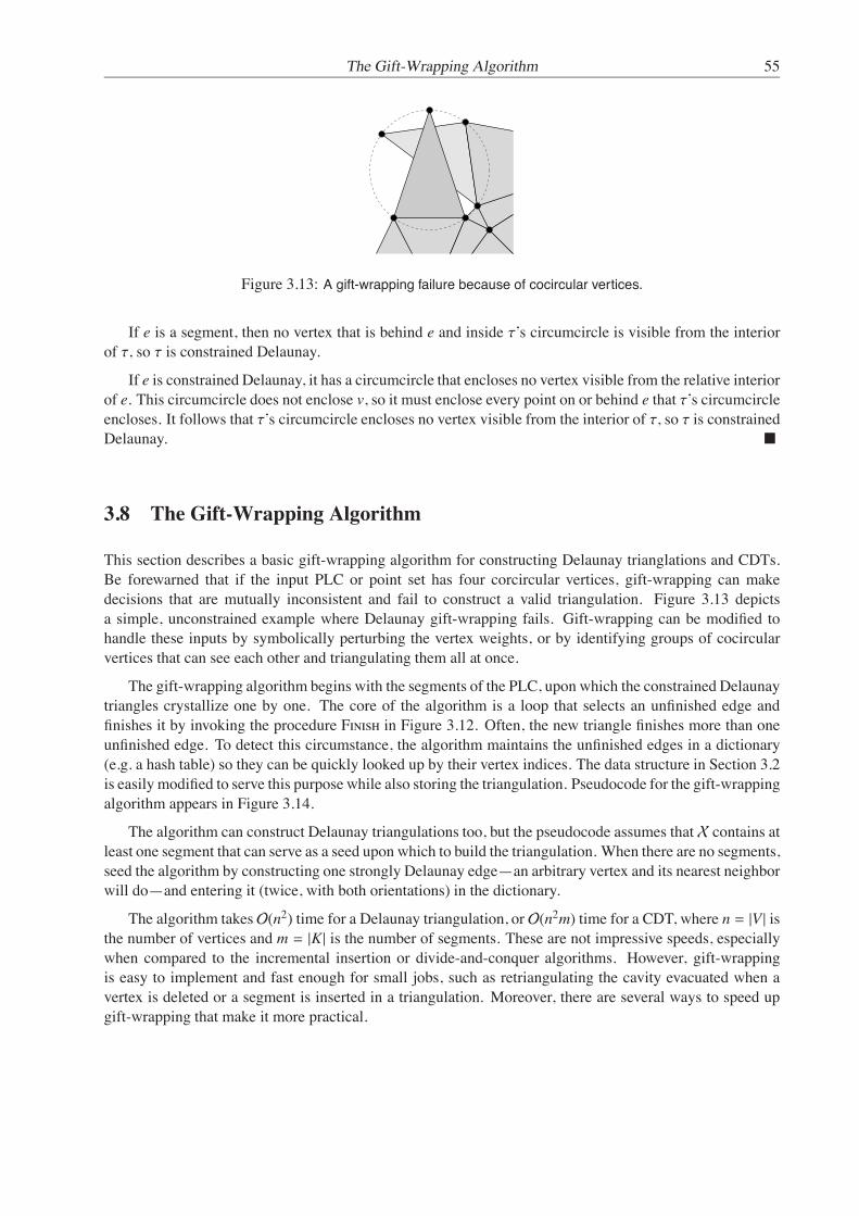
The Gift-Wrapping Algorithm 55
Figure 3.13: A gift-wrapping failure because of cocircular vertices.
If e is a segment, then no vertex that is behind e and inside τ’s circumcircle is visible from the interiorof τ, so τ is constrained Delaunay.
If e is constrained Delaunay, it has a circumcircle that encloses no vertex visible from the relative interiorof e. This circumcircle does not enclose v, so it must enclose every point on or behind e that τ’s circumcircleencloses. It follows that τ’s circumcircle encloses no vertex visible from the interior of τ, so τ is constrainedDelaunay. "
3.8 The Gift-Wrapping Algorithm
This section describes a basic gift-wrapping algorithm for constructing Delaunay trianglations and CDTs.Be forewarned that if the input PLC or point set has four corcircular vertices, gift-wrapping can makedecisions that are mutually inconsistent and fail to construct a valid triangulation. Figure 3.13 depictsa simple, unconstrained example where Delaunay gift-wrapping fails. Gift-wrapping can be modified tohandle these inputs by symbolically perturbing the vertex weights, or by identifying groups of cocircularvertices that can see each other and triangulating them all at once.
The gift-wrapping algorithm begins with the segments of the PLC, upon which the constrained Delaunaytriangles crystallize one by one. The core of the algorithm is a loop that selects an unfinished edge andfinishes it by invoking the procedure Finish in Figure 3.12. Often, the new triangle finishes more than oneunfinished edge. To detect this circumstance, the algorithm maintains the unfinished edges in a dictionary(e.g. a hash table) so they can be quickly looked up by their vertex indices. The data structure in Section 3.2is easily modified to serve this purpose while also storing the triangulation. Pseudocode for the gift-wrappingalgorithm appears in Figure 3.14.
The algorithm can construct Delaunay triangulations too, but the pseudocode assumes that X contains atleast one segment that can serve as a seed upon which to build the triangulation. When there are no segments,seed the algorithm by constructing one strongly Delaunay edge—an arbitrary vertex and its nearest neighborwill do—and entering it (twice, with both orientations) in the dictionary.
The algorithm takes O(n2) time for a Delaunay triangulation, or O(n2m) time for a CDT, where n = |V | isthe number of vertices and m = |K| is the number of segments. These are not impressive speeds, especiallywhen compared to the incremental insertion or divide-and-conquer algorithms. However, gift-wrappingis easy to implement and fast enough for small jobs, such as retriangulating the cavity evacuated when avertex is deleted or a segment is inserted in a triangulation. Moreover, there are several ways to speed upgift-wrapping that make it more practical.

56 Jonathan Richard Shewchuk
GiftWrapCDT(V,K) V is the set of vertices in a PLC X. K is the set of segments in X. 1 for each segment s ∈ K that adjoins a wall on one side only2 Enter s in the dictionary, oriented so its front adjoins a wall3 while the dictionary is not empty
Loop invariant: the dictionary contains all the unfinished edges. 4 Remove an oriented edge e from the dictionary5 τ← Finish(e,V,K)6 if τ ! ∅7 AddTriangle(t)8 for each oriented edge f of τ except e9 if f is in the dictionary10 Remove f from the dictionary11 else Enter f in the dictionary with reversed orientation
(facing away from τ)
Figure 3.14: Gift-wrapping algorithm for constructing a CDT.
One specialized class of gift-wrapping algorithms are sweepline algorithms that construct the trianglesin a disciplined order, making it possible to determine which vertex finishes each edge without an exhaustivesearch. Fortune [51] developed such an algorithm for Delaunay triangulations. Seidel [109] extended it toCDTs. Both algorithms run in O(n log n) time.
Another way to avoid exhaustive search is to subdivide the plane into square buckets, record the ver-tices in their respective buckets, and finish each edge by searching through the buckets in an appropriateorder. Dwyer [47] shows that if the vertices are distributed uniformly at random in a disk, this techniquefinishes each face in O(1) expected time, so an entire Delaunay triangulation can be constructed in O(n)expected time. Moreover, the algorithm extends to higher dimensions, still with expected linear runningtime! Unfortunately, this method does not extend easily to CDTs, and not all real-world point sets are sonicely distributed. It is easy to construct a point set for which most of the points fall into one bucket.
3.9 Inserting a Segment into a Constrained Delaunay Triangulation
To “insert a segment into a CDT” is to take as input the CDT of a PLC X and a new segment s to insert, andproduce the CDT of X ∪ s. It is only meaningful if X ∪ s is a valid PLC—that is, X already contains thevertices of s (otherwise, they must be inserted first, as described in Section 3.6), and the relative interior of sintersects no segment or vertex in X. This section presents a gift-wrapping algorithm for segment insertion.It appears in an article by Anglada [3], but it was part of the folklore of the field before that paper appeared.It is difficult to trace who thought of the algorithm first.
Let T be the CDT of X. If s ∈ T , then T is also the CDT of X ∪ s. Otherwise, the algorithm beginsby deleting from T the edges and triangles that intersect the relative interior of s. All of T ’s simplices notdeleted remain constrained Delaunay after s is inserted. Next, the algorithm adds s to the complex, and itretriangulates the two polygonal cavities on each side of s with constrained Delaunay triangles. Recall fromFigure 2.16 that the cavities might have segments dangling in their interiors.
Let P be one of the two polygons; its edges include s. The algorithm GiftWrapCDT could gift-wrapP starting from any edge of P, but there are several advantages to gift-wrapping from s outward. First,

Inserting a Segment into a Constrained Delaunay Triangulation 57
s wv
uu w
Figure 3.15: Gift-wrapping one triangle from a newly inserted segment s.
gift-wrapping from s makes it possible to eliminate the visibility tests (Line 5 of Finish) and the dictionaryof unfinished edges, speeding up the algorithm by a factor of m. Second, gift-wrapping from s gives thebest likelihood of subdividing P into two half-sized polygons, improving the speed of the algorithm. Third,the algorithm is guaranteed to work correctly even if X has four or more cocircular vertices. Be forewarnedthat gift-wrapping without visibility tests does not work correctly for all polygons, but it works for segmentinsertion.
The cavity retriangulation algorithm is as follows. Begin by gift-wrapping one constrained Delaunaytriangle in front of s, as illustrated in Figure 3.15. Let u and w be the vertices of s, and let uwv be thepositively oriented triangle produced by the gift-wrapping step. The cavity retriangulation algorithm callsitself recursively on the oriented edges uv and vw (if they are unfinished).
The running time of the first gift-wrapping step is proportional to the number m of vertices of P. Ifwe are lucky, it will split P into two polygons of roughly half the size, and the recursive calls will alsoenjoy balanced splits, so the time required to triangulate P will be in O(m log m). In the worst case, eachgift-wrapping step might simply cut one triangle off of P without subdividing P into smaller polygons, andit will take Θ(m2) time to triangulate P. In practice, if m is large, P is probably long and thin and will enjoywell-balanced recursive calls.


Chapter 4
Three-Dimensional DelaunayTriangulations
Three-dimensional triangulations are sometimes called tetrahedralizations. Delaunay tetrahedralizations arenot quite as effective as planar Delaunay triangulations at producing elements of good quality, but they arenearly as popular in the mesh generation literature as their two-dimensional cousins. Many properties ofDelaunay triangulations in the plane generalize to higher dimensions, but many of the optimality propertiesdo not. Notably, Delaunay tetrahedralizations do not maximize the minimum angle (whether plane angleor dihedral angle). Figure 4.1 depicts a three-dimensional counterexample. The hexahedron at the top isthe convex hull of its five vertices. The Delaunay triangulation of those vertices, to the left, includes a thintetrahedron known as a sliver or kite, whose vertices are nearly coplanar and whose dihedral angles can bearbitrarily close to 0 and 180. A triangulation of the same vertices that is not Delaunay, at lower right, hasbetter quality.
This chapter surveys Delaunay triangulations and constrained Delaunay triangulations in three (and oc-casionally more) dimensions. Constrained Delaunay triangulations generalize uneasily to three dimensions,because there are polyhedra that do not have any tetrahedralization at all.
Figure 4.1: This hexahedron has two tetrahedralizations. The Delaunay tetrahedralization at left includes anarbitrarily thin sliver tetrahedron. The non-Delaunay tetrahedralization at right consists of two nicely shapedtetrahedra.
59
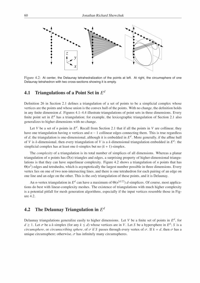
60 Jonathan Richard Shewchuk
yz
x
Figure 4.2: At center, the Delaunay tetrahedralization of the points at left. At right, the circumsphere of oneDelaunay tetrahedron with two cross-sections showing it is empty.
4.1 Triangulations of a Point Set in Ed
Definition 26 in Section 2.1 defines a triangulation of a set of points to be a simplicial complex whosevertices are the points and whose union is the convex hull of the points. With no change, the definition holdsin any finite dimension d. Figures 4.1–4.4 illustrate triangulations of point sets in three dimensions. Everyfinite point set in Ed has a triangulation; for example, the lexicographic triangulation of Section 2.1 alsogeneralizes to higher dimensions with no change.
Let V be a set of n points in Ed. Recall from Section 2.1 that if all the points in V are collinear, theyhave one triangulation having n vertices and n − 1 collinear edges connecting them. This is true regardlessof d; the triangulation is one-dimensional, although it is embedded in Ed. More generally, if the affine hullof V is k-dimensional, then every triangulation of V is a k-dimensional triangulation embedded in Ed: thesimplicial complex has at least one k-simplex but no (k + 1)-simplex.
The complexity of a triangulation is its total number of simplices of all dimensions. Whereas a planartriangulation of n points has O(n) triangles and edges, a surprising property of higher-dimensional triangu-lations is that they can have superlinear complexity. Figure 4.2 shows a triangulation of n points that hasΘ(n2) edges and tetrahedra, which is asymptotically the largest number possible in three dimensions. Everyvertex lies on one of two non-intersecting lines, and there is one tetrahedron for each pairing of an edge onone line and an edge on the other. This is the only triangulation of these points, and it is Delaunay.
An n-vertex triangulation in Ed can have a maximum of Θ(n⌈d/2⌉) d-simplices. Of course, most applica-tions do best with linear-complexity meshes. The existence of triangulations with much higher complexityis a potential pitfall for mesh generation algorithms, especially if the input vertices resemble those in Fig-ure 4.2.
4.2 The Delaunay Triangulation in Ed
Delaunay triangulations generalize easily to higher dimensions. Let V be a finite set of points in Ed, ford ≥ 1. Let σ be a k-simplex (for any k ≤ d) whose vertices are in V . Let S be a hypersphere in Ed; S is acircumsphere, or circumscribing sphere, of σ if S passes through every vertex of σ. If k = d, then σ has aunique circumsphere; otherwise, σ has infinitely many circumspheres.

The Delaunay Triangulation in Ed 61
Figure 4.3: Three renderings of a Delaunay tetrahedralization.
Figure 4.4: A Delaunay subdivision comprising two cubic cells and their faces. The least-vertex Delaunaytriangulation subdivides each 2-face into triangles adjoining the face’s lexicographically minimum vertex, andlikewise subdivides each 3-face into tetrahedra.
A simplex σ is Delaunay if there exists a circumsphere of σ that encloses no point in V . Clearly, everyface of a Delaunay simplex is Delaunay too. A simplex σ is strongly Delaunay if there exists a circumsphereS of σ such that no point in V lies inside or on S , except the vertices of σ. Every point in V is triviallya strongly Delaunay vertex. A Delaunay triangulation Del V of V is a triangulation of V in which everyd-simplex is Delaunay, as Figure 4.2 shows. Figure 4.3 depicts a more typical Delaunay tetrahedralization,with complexity linear in the number of vertices.
The parabolic lifting map generalizes to higher dimensions too. It maps each point p = (p1, p2, . . . , pd) ∈Ed to its lifted companion, the point p+ = (p1, p2, . . . , pd, p2
1 + p22 + · · · + p2
d) in Ed+1. Consider the (d +1)-dimensional convex hull of the lifted points, V+ = v+ : v ∈ V. Projecting the downward-facingfaces of conv(V+) to Ed yields a polyhedral complex called the Delaunay subdivision of V , which is easilytransformed to its complement, the Voronoi diagram of V .
If V is generic, its Delaunay subdivision is simplicial and V has exactly one Delaunay triangulation,
Definition 39 (generic). Let V be a point set in Ed. Let k be the dimension of the affine hull of V. V isgeneric if no k + 2 points in V lie on a common hypersphere.
If V if not generic, the Delaunay subdivision may have non-simplicial faces; recall Figure 2.4. In thatcase, V has multiple Delaunay triangulations, which differ according to how the non-simplicial faces aretriangulated.
Whereas each non-simplicial face in a two-dimensional Delaunay subdivision can be triangulated inde-pendently, in higher dimensions the triangulations are not always independent. Figure 4.4 illustrates a setof twelve points in E3 whose Delaunay subdivision includes two cubic cells that share a square 2-face. Thesquare face can be divided into two triangles in two different ways, and each cube can be divided into five orsix tetrahedra in several ways, but they are not independent: the triangulation of the square face constrainshow both cubes are triangulated.

62 Jonathan Richard Shewchuk
A least-vertex triangulation provides one way to safely subdivide a polyhedral complex into a simplicialcomplex. To construct it, triangulate the 2-faces through the d-faces in order of increasing dimension. Totriangulate a non-simplicial k-face f , subdivide it into k-simplices of the form conv(v ∪ g), where v is thelexicographically minimum vertex of f , and g varies over the (k − 1)-simplices on f ’s subdivided boundarythat do not contain v. The choice of the lexicographically minimum vertex of each face ensures that the facetriangulations are compatible with each other.
4.3 Properties of Delaunay Triangulations in Ed
Many properties of planar Delaunay triangulations discussed in Chapter 2 generalize to higher dimensions.A few of them are summarized below. Proofs are omitted, but each of them is a straightforward extensionof the corresponding proof for two dimensions.
Recall that a facet of a polyhedral complex is a (d − 1)-face, and a facet of a triangulation is a (d − 1)-simplex. The Delaunay Lemma provides an alternative definition of a Delaunay triangulation: a triangu-lation of a point set in which every facet is locally Delaunay. A facet f in a triangulation T is said to belocally Delaunay if it is a face of fewer than two d-simplices in T , or it is a face of exactly two d-simplicesτ1 and τ2 and it has a circumsphere enclosing no vertex of τ1 nor τ2. (Equivalently, the circumsphere of τ1encloses no vertex of τ2. Equivalently, the circumsphere of τ2 encloses no vertex of τ1.)
Theorem 23 (Delaunay Lemma). Let T be a triangulation of a finite set V of points in Ed. The followingthree statements are equivalent.
• Every d-simplex in T is Delaunay (i.e. T is Delaunay).
• Every facet in T is Delaunay.
• Every facet in T is locally Delaunay. "
As in the plane, a generic point set has exactly one Delaunay triangulation, composed of every stronglyDelaunay simplex. The following three theorems have essentially the same proofs as in Section 2.7.
Theorem 24. Let σ be a strongly Delaunay simplex, and let τ be a Delaunay simplex. Then σ ∩ τ is eitherempty or a shared face of both σ and τ.
Theorem 25. Every Delaunay triangulation of a point set contains every strongly Delaunay simplex.
Corollary 26. A generic point set has exactly one Delaunay triangulation.
4.4 The Optimality of the Delaunay Triangulation in Ed
Some optimality properties of Delaunay triangulations hold in any dimension. Rippa [98] investigates theuse of two-dimensional triangulations for piecewise linear interpolation of a quadratic bivariate function. Ifthe function is isotropic—of the form α(x2 + y2) + βx + γy + δ—then the Delaunay triangulation minimizesthe interpolation error measured in the Lq-norm for every q ≥ 1, compared with all other triangulations ofthe same points. Melissaratos [80] generalizes Rippa’s result to higher dimensions. (If the function is notisotropic, but it is parabolic rather than hyperbolic, then the optimal triangulation is a weighted Delaunaytriangulation in which the function determines the vertex heights.)

The Optimality of the Delaunay Triangulation in Ed 63
D’Azevedo and Simpson [42] show that a two-dimensional Delaunay triangulation minimizes the radiusof the largest min-containment circle of its simplices, and Rajan [96] generalizes this result to Delaunay tri-angulations and min-containment spheres of any dimensionality. The min-containment sphere of a simplexis the smallest hypersphere that encloses the simplex.
Rajan’s result and a theorem of Waldron [127] together imply a third optimality result, also relatedto multivariate piecewise linear interpolation. Suppose you must choose a triangulation to interpolate anunknown function, and you wish to minimize the largest pointwise error in the domain. After you choosethe triangulation, an adversary will choose the worst possible smooth function for your triangulation tointerpolate, subject to a fixed upper bound on the absolute curvature (i.e. second directional derivative) ofthe function anywhere in the domain. The Delaunay triangulation is your optimal choice.
To better understand these three optimality properties, consider multivariate piecewise linear interpola-tion on a triangulation T of a point set V . Let T + = σ+ : σ ∈ T be the triangulation lifted by the paraboliclifting map; T + is a simplicial complex embedded in Ed+1. Think of T + as inducing a continuous piecewiselinear function T +(p) that maps each point p ∈ conv(V) to a real value.
How well does T + approximate the paraboloid? Let e(p) = T +(p) − |p|2 be the error in the interpolatedfunction T + as an approximation of the paraboloid |p|2. At each vertex v ∈ V , e(v) = 0. Because |p|2 isconvex, the error satisfies e(p) ≥ 0 for all p ∈ conv(V).
Theorem 27. At every point p ∈ conv(V), every Delaunay triangulation T of V minimizes T +(p), andtherefore minimizes the interpolation error e(p), among all triangulations of V.
Proof. If T is Delaunay, then T + is the set of faces of the underside of the convex hull conv(V+) of thelifted vertices (or a subdivision of those faces if some of them are not simplicial). No triangulation whosevertices are V+ can pass through any point below conv(V+). "
Corollary 28 (Melissaratos [80]). Every Delaunay triangulation of V minimizes ∥e∥Lq for every Lebesguenorm Lq, and every other norm monotonic in e. "
Theorem 29 (Rajan [96]). Every Delaunay triangulation of V minimizes the largest min-containment sphere,compared with all other triangulations of V. "
I omit the proof because of its length.The optimality of the Delaunay triangulation for controlling the largest min-containment radius dovetails
nicely with an error bound for piecewise linear interpolation derived by Waldron [127]. Let Cc be the spaceof scalar functions defined over conv(V) that have C1 continuity and whose absolute curvature nowhereexceeds c. In other words, for every f ∈ Cc, every point p ∈ conv(V), and every unit direction vector d,the magnitude of the second directional derivative f ′′d (p) is at most c. This is a common starting point foranalyses of piecewise linear interpolation error.
Let f be a function in Cc. Let σ ⊆ conv(V) be a simplex (of any dimensionality) with min-containmentradius rmc. Let hσ be a linear function that interpolates f at the vertices of σ. Waldron shows that for allp ∈ σ, the absolute error |e(p)| = |hσ(p) − f (p)| is at most cr2
mc/2. Furthermore, this bound is sharp: forevery simplex σ with min-containment radius rmc, there is a function f ∈ Cc and a point p ∈ σ such that|e(p)| = cr2
mc/2. That function is f (p) = c|p|2/2, and that point is p = Omc.
Theorem 30. Every Delaunay triangulation T of V minimizes
maxf∈Cc
maxp∈conv(V)
|T +(p) − f (p)|,
the worst-case pointwise interpolation error, among all triangulations of V.

64 Jonathan Richard Shewchuk
Figure 4.5: Schonhardt’s untetrahedralizable polyhedron (center) is formed by rotating one end of a triangularprism (left), thereby creating three diagonal reflex edges. The convex hull of any four polyhedron vertices (right)sticks out.
Proof. For any triangulation T , max f∈Cc maxp∈conv(V) |T +(p) − f (p)| = cr2max/2, where rmax is the largest
min-containment radius among all the simplices in T . The result follows immediately from Theorem 29. "
One of the reasons why Delaunay triangulations are important is because, in the senses of Theorems 27and 30, the Delaunay triangulation is an optimal piecewise linear interpolating surface. Of course, e(p) isnot the only criterion for the merit of a triangulation used for interpolation. Many applications need theinterpolant to approximate the gradient—that is, not only must T +(p) approximate f (p), but ∇T +(p) mustapproximate∇ f (p) well too. For the goal of approximating∇ f (p) in three or more dimensions, the Delaunaytrianguation is sometimes far from optimal even for simple functions like the paraboloid f (p) = |p|2. Thisis why eliminating slivers is a crucial problem in Delaunay mesh generation.
4.5 Three-Dimensional Constrained Delaunay Triangulations
Constrained Delaunay triangulations generalize to three or more dimensions, but whereas every piecewiselinear complex in the plane has a CDT, not every three-dimensional PLC has one. Worse yet, there existsimple polyhedra that do not have triangulations at all—that is, they cannot be subdivided into tetrahedrawithout creating new vertices (i.e. tetrahedron vertices that are not vertices of the polyhedron).
E. Schonhardt [106] furnishes an example depicted in Figure 4.5. The easiest way to envision thispolyhedron is to begin with a triangular prism. Imagine grasping the prism so that its bottom triangular facecannot move, while twisting the top triangular face so it rotates slightly about its center while remaininghorizontal. This rotation breaks each of the three square faces into two triangular faces along a diagonalreflex edge—an edge at which the polyhedron is locally nonconvex. After this transformation, the upper leftcorner and lower right corner of each (former) square face are separated by a reflex edge and are no longervisible to each other within the polyhedron. Any four vertices of the polyhedron include two separated by areflex edge; thus, any tetrahedron whose vertices are vertices of the polyhedron does not lie entirely withinthe polyhedron. Therefore, Schonhardt’s polyhedron cannot be triangulated without additional vertices. Itcan be subdivided into tetrahedra with the addition of one vertex at its center.
Adding to the difficulty, Ruppert and Seidel [103] prove that it is NP-hard to determine whether apolyhedron has a triangulation, or whether it can be subdivided into tetrahedra with only k additional verticesfor an arbitrary constant k.
The following sections discuss triangulations and CDTs of polyhedra and PLCs in three dimensions. Itis possible to refine any polyhedron or PLC by adding new vertices on its edges so that it has a constrainedDelaunay triangulation. This fact makes CDTs useful in three dimensions.

Three-Dimensional Constrained Delaunay Triangulations 65
Figure 4.6: A three-dimensional piecewise linear complex and its constrained Delaunay triangulation. Eachpolygon and polyhedron may have holes, slits, and vertices in its relative interior. Each polyhedron may also havepolygons in its interior.
4.5.1 Piecewise Linear Complexes and their Triangulations in Ed
The domain over which a general-dimensional CDT is defined is a general-dimensional piecewise linearcomplex, which is a set of linear cells—points, edges, polygons, and polyhedra—as illustrated in Figure 4.6.The linear cells constrain how the complex can be triangulated: each linear cell in the complex must be aunion of simplices in the triangulation. The union of the linear cells specifies the region to be triangulated.
Definition 40 (piecewise linear complex; segment; wall; face). A piecewise linear complex (PLC) X is afinite set of linear cells that satisfies the following properties.
• The vertices and edges in X form a simplicial complex.
• For each linear cell f ∈ X, the boundary of f is a union of linear cells in X.
• If two distinct linear cells f , g ∈ X intersect, their intersection is a union of linear cells in X, allhaving lower dimension than at least one of f or g. (See Figures 2.14 and 4.6.)
As in the plane, X’s edges are called segments and its polygons are called walls. Its underlying space is|X| =
"
f∈X f , which is usually the domain to be triangulated. The faces of a linear cell f ∈ X are the linearcells in X that are subsets of f , including f itself.
The notion of a PLC was proposed by Miller, Talmor, Teng, Walkington, and Wang [82].1 A triangula-tion of a PLC must cover every polyhedron, respect every polygon, and include every segment.
Definition 41 (triangulation of a PLC). Let X be a PLC. A triangulation of X is a simplicial complex T suchthat
• X and T have the same vertices,
• every linear cell in X is a union of simplices in T (which implies that every edge in X is in T ), and
• |T | = |X|.1Miller et al. call it a piecewise linear system, but their construction is so obviously a complex that a change in name seems
obligatory. The present definition is different from Miller’s, but nearly equivalent, with one true difference: Miller does not imposethe first condition given here, but permits vertices to lie in the relative interior of an edge. Disallowing such vertices simplifies thepresentation while entailing no essential loss of generality, because edges with vertices in their relative interiors can be subdividedinto edges that obey the condition.

66 Jonathan Richard Shewchuk
Figure 4.7: A convex PLC with no triangulation.
Figure 4.8: Chazelle’s polyhedron.
Schonhardt’s polyhedron shows that not every PLC has a triangulation. Every convex polyhedron hasa triangulation; what about convex polyhedra with internal segments? Figure 4.7 illustrates a PLC with notriangulation, consisting of a cube inside which three orthogonal segments pass by each other but do notintersect. If any one of the segments is omitted, the PLC has a triangulation. This example shows that,unlike with planar triangulations, it is not always possible to insert a new edge into a tetrahedralization.
Because some polyhedra and PLCs do not have triangulations, Steiner triangulations (Definition 35) areeven more important in three dimensions than in the plane. Chazelle [27] shows that every n-vertex polyhe-dron has a Steiner triangulation with at most O(n2) vertices, found by constructing a vertical decompositionof the polyhedron. The same is true for PLCs of complexity n. Unfortunately, there are polyhedra for whichit is not possible to do better; Figure 4.8 depicts Chazelle’s polyhedron [27], which has n vertices and O(n)edges, but cannot be divided into fewer than Θ(n2) convex bodies. Chazelle and Palios [28] show that theworst-case complexity of subdividing a polyhedron is related to its number of reflex edges: they give analgorithm that divides any polyhedron with r reflex edges into O(n+ r2) tetrahedra, and they show that somepolyhedra with r reflex edges cannot be divided into fewer than Ω(n + r2) convex bodies.
It appears likely, though it is proven only in two dimensions, that there exist PLCs whose smallest SteinerDelaunay triangulations are asymptotically larger than their smallest Steiner triangulations. Algorithms byMurphy, Mount, and Gable [87], Cohen-Steiner, Colin de Verdiere, and Yvinec [40], Cheng and Poon [33],and Rand and Walkington [97] can find a Steiner Delaunay tetrahedralization of any three-dimensionalpolyhedron, but they might introduce a superpolynomial number of new vertices. No known algorithmfor finding Steiner Delaunay tetrahedralizations is guaranteed to introduce only a polynomial number ofnew vertices, and no algorithm of any complexity has been offered for four- or higher-dimensional SteinerDelaunay triangulations. Moreover, the existing algorithms all seem to introduce an unnecessarily largenumber of vertices near small domain angles. These problems can be partly remediated by Steiner CDTs.

Three-Dimensional Constrained Delaunay Triangulations 67
τ v
f
Figure 4.9: A constrained Delaunay tetrahedron τ.
4.5.2 The Constrained Delaunay Triangulation in E3
Three-dimensional constrained Delaunay triangulations aspire to retain most of the advantages of Delaunaytriangulations while respecting constraints. But Figures 4.5, 4.7, and 4.8 demonstrate that some PLCs, evensome polyhedra, have no triangulation at all. Moreover, some polyhedra that do have triangulations do nothave CDTs. Nevertheless, CDTs are useful because, if we are willing to add new vertices, a Steiner CDTmight require many fewer vertices than a Steiner Delaunay triangulation.
As in the plane, a Constrained Delaunay Lemma states that there are several equivalent definitions of“constrained Delaunay triangulation.” The simplest is that a CDT is a triangulation of a PLC in which everyfacet not included in a wall is locally Delaunay. A CDT differs from a Delaunay triangulation in three ways:it is not necessarily convex, it is required to respect a PLC, and the facets of the CDT that are included inwalls are exempt from being locally Delaunay.
The primary definition of CDT specifies that every tetrahedron is constrained Delaunay, defined asfollows.
Definition 42 (constrained Delaunay). In the context of a PLC X, a simplex σ is constrained Delaunay if itsatisfies the following three conditions.
• X contains σ’s vertices.
• σ respects X. (Recall Definition 34.)
• There is a circumsphere of σ that encloses no vertex in X that is visible from any point in the relativeinterior of σ.
Two points are visible to each other (equivalently, can see each other) if |X| includes the open linesegment connecting the two points, but no linear cell in X intersects only part of that open line segment. Alinear cell that intersects the open line segment but does not entirely include it is said to occlude the visibilitybetween the two points.
Figure 4.9 depicts a constrained Delaunay tetrahedron τ. The faces of τ whose relative interiors intersectthe wall f are included in f , so τ respectsX. The circumsphere of τ encloses one vertex v, but v is not visiblefrom any point in the interior of τ, because f occludes its visibility.
Definition 43 (constrained Delaunay triangulation). A constrained Delaunay triangulation (CDT) of a PLCX is a triangulation of X in which every tetrahedron is constrained Delaunay, and every triangle that is nota face of a tetrahedron is constrained Delaunay.

68 Jonathan Richard Shewchuk
Figure 4.10: Left: a PLC with no CDT. Center: the sole tetrahedralization of this PLC. Its three tetrahedra arenot constrained Delaunay. Right: the two Delaunay tetrahedra do not respect the central segment.
Figure 4.6 illustrates a PLC and its CDT. Observe that the PLC has a polygon that is not a face of anypolyhedron; this face is triangulated with constrained Delaunay triangles.
Figure 4.10 illustrates a PLC that has no CDT because of a segment that runs vertically through thedomain interior. There is only one tetrahedralization of this PLC—composed of three tetrahedra encirclingthe central segment—and its tetrahedra are not constrained Delaunay, because each of them has a visiblevertex inside its circumsphere. Whereas walls usually block enough visibility to ensure their presence ina CDT, segments usually do not. But segments can dictate that a CDT does not exist at all. If the centralsegment in Figure 4.10 is removed, the PLC has a CDT made up of two tetrahedra.
A Steiner CDT or conforming CDT of X is a Steiner triangulation of X in which every tetrahedronis constrained Delaunay, and every triangle that is not a face of a tetrahedron is constrained Delaunay.Algorithms for constructing Steiner CDTs (e.g. mesh generation algorithms) must sometimes place newvertices on segments to force the triangulation to respect them.
4.5.3 The CDT Theorem
Although not all piecewise linear complexes have constrained Delaunay triangulations, there is an easilytested, sufficient (but not necessary) condition that guarantees that a CDT exists. A three-dimensional PLCX is edge-protected if every edge in X is strongly Delaunay.
Theorem 31 (CDT Theorem [118]). Every edge-protected PLC has a CDT. #
It is not sufficient for every edge inX to be Delaunay. If all six vertices of Schonhardt’s polyhedron lie ona common sphere, then all of its edges (and all its faces) are Delaunay, but it still has no tetrahedralization.It is not possible to place the vertices of Schonhardt’s polyhedron so that all three of its reflex edges arestrongly Delaunay, though any two may be.
What if a PLC that you wish to triangulate is not edge-protected? You can make it edge-protected byadding vertices on its segments—a task that any Delaunay mesh generation algorithm must do anyway. Theaugmented PLC has a CDT, which is a Steiner CDT of the original PLC.
Figure 4.11 illustrates the difference between using a Delaunay triangulation and using a CDT for meshgeneration. With a Delaunay triangulation, the mesh generator must insert new vertices that guarantee thatevery segment is a union of Delaunay (preferably strongly Delaunay) edges, and every wall is a unionof Delaunay (preferably strongly Delaunay) triangles. With a CDT, new vertices must be inserted thatguarantee that every segment is a union of strongly Delaunay edges; but then the augmented PLC is edge-protected, and the CDT Theorem guarantees that the walls can be recovered without inserting any additionalvertices. The advantage of a CDT is that many fewer vertices might be required.

Three-Dimensional Constrained Delaunay Triangulations 69
Steiner DT
Steiner CDT
Figure 4.11: Comparison of Steiner Delaunay triangulations and Steiner CDTs. For clarity, vertices inside eachbox are shown, but tetrahedra are not. For both types of triangulation, missing segments are recovered by insert-ing new vertices until each segment is a union of strongly Delaunay edges. In a Steiner Delaunay triangulation,additional vertices are inserted until each wall is a union of strongly Delaunay triangles. In a Steiner CDT, noadditional vertices need be inserted; the walls are recovered by computing a CDT.
Testing whether a PLC X is edge-protected is straightforward. Form the Delaunay triangulation of thevertices in X. If a segment s ∈ X is missing from the triangulation, then s is not strongly Delaunay, andX is not edge-protected. If s is present, it is Delaunay. Testing whether a Delaunay segment s is stronglyDelaunay is equivalent to determining whether the Voronoi polygon dual to s is nondegenerate.
4.5.4 Properties of the Constrained Delaunay Triangulation in E3
This section summarizes the properties of three-dimensional CDTs. Proofs of the claims in this section maybe found elsewhere [118].
The Delaunay Lemma for three-dimensional CDTs provides an alternative definition of CDT: a triangu-lation of a PLC X is a CDT if and only if every one of its facets is locally Delaunay or is included in a wallin X.
Theorem 32 (Constrained Delaunay Lemma). Let X be a PLC in which every linear cell is a face of somepolyhedron in X, so there are no dangling polygons. Let T be a triangulation of X. The following threestatements are equivalent.
A. Every tetrahedron in T is constrained Delaunay (i.e. T is constrained Delaunay).
B. Every facet in T not included in a wall in X is constrained Delaunay.
C. Every facet in T not included in a wall in X is locally Delaunay. "
A constrained Delaunay triangulation T of X induces a two-dimensional triangulation of each wallf ∈ X, namely T | f = σ ∈ T : σ ⊆ f . Statement B above implies that the triangles in T | f need not beconstrained Delaunay with respect to X—but they are constrained Delaunay with respect to the wall f , inthe following sense.
Theorem 33. Let T be a CDT of a three-dimensional PLC X. Let f ∈ X be a wall. Let T | f be the setof simplices in T that are included in f . Let X| f be the set of faces of f (including f itself); X| f is atwo-dimensional PLC embedded in three-dimensional space. Then T | f is a CDT of X| f . "
A PLC is generic if its vertices are generic. A generic PLC has a unique CDT, if it has one at all.

70 Jonathan Richard Shewchuk
Theorem 34. A generic piecewise linear complex has at most one constrained Delaunay triangulation. "
A consequence of Theorems 33 and 34 is that, if a PLC is generic, a CDT construction algorithm canbegin by computing the two-dimensional CDTs of the walls, then use them to help compute the three-dimensional CDT of the PLC, secure in the knowledge that the wall triangulations will match the volumetriangulation.
CDTs inherit the optimality properties of Delaunay triangulations described in Section 4.4, albeit withrespect to a smaller set of triangulations, namely the triangulations of a PLC. However, if a PLC has noCDT, finding the optimal triangulation is an open problem.
Theorem 35. If a PLC X has a CDT, then every CDT of X minimizes the largest min-containment sphere,compared with all other triangulations of X. Every CDT of X also optimizes the criteria discussed inTheorems 27, 28, and 30. "

Chapter 5
Algorithms for Constructing DelaunayTriangulations in E3
The most popular algorithms for constructing Delaunay tetrahedralizations are incremental insertion andgift-wrapping algorithms, both of which generalize to three or more dimensions with little difficulty. Thischapter reprises those algorithms, with attention to the aspects that are different in three dimensions. Inparticular, the analysis of the running time of point location with conflict lists is more complicated in threedimensions than in the plane. I use this gap as an opportunity to introduce a more sophisticated vertexordering and its analysis. Instead of fully randomizing the order in which vertices are inserted, I recommendusing a biased randomized insertion order that employs just enough randomness to ensure that the expectedrunning time is the worst-case optimalO(n2)—or better yet, O(n log n) time for the classes of point sets mostcommonly triangulated in practice—while maintaining enough spatial locality that implementations of thealgorithm use the memory hierarchy more efficiently. This vertex ordering, combined with a simpler pointlocation method, yields the fastest three-dimensional Delaunay triangulators in practice.
CDTs have received much less study in three dimensions than in two. There are two classes of algorithmavailable: gift-wrapping and incremental wall insertion. Gift-wrapping is easier to implement; it is not muchdifferent in three dimensions than in two. It runs in O(nh) time for Delaunay triangulations and O(nmh) timefor CDTs, where n is the number of vertices, m is the total complexity of the PLC’s polygons, and h is thenumber of tetrahedra produced. There is a variant of the gift-wrapping algorithm that, by constructing thetetrahedra in a disciplined order and using other tricks to avoid visibility computations [115], runs in O(nh)worst-case time, but I omit it here.
Perhaps the fastest three-dimensional CDT construction algorithm in practice is similar to the one Iadvocate in two dimensions. First, construct a Delaunay triangulation of the PLC’s vertices, then insert itswalls one by one with a flip algorithm [117]. This algorithm constructs a CDT in O(n2 log n) time, thoughthere are reasons to believe it will run in O(n log n) time on most PLCs in practice. Be forewarned, however,that this algorithm only works on edge-protected PLCs! This is rarely a fatal restriction, because a meshgeneration algorithm that uses CDTs should probably insert vertices on the PLC’s edges to make it edge-protected and ensure that it has a CDT. Some PLCs have CDTs despite not being edge-protected; if they aregeneric, their CDTs can be constructed by gift-wrapping.
71

72 Jonathan Richard Shewchuk
Procedure PurposeAddTetrahedron(u, v,w, x) Add a positively oriented tetrahedron uvwxDeleteTetrahedron(u, v,w, x) Delete a positively oriented tetrahedron uvwxAdjacent(u, v,w) Return a vertex x such that uvwx is a positively oriented tetrahedronAdjacentOne(u) Return vertices v, w, x such that uvwx is a positively oriented tetrahedron
Figure 5.1: An interface for a tetrahedralization data structure.
5.1 A Dictionary Data Structure for Tetrahedralizations
Figure 5.1 summarizes an interface for storing a tetrahedral complex, analogous to the interface for planartriangulations in Section 3.2. Two procedures, AddTetrahedron and DeleteTetrahedron, specify a tetra-hedron to be added or deleted by listing its vertices with a positive orientation, as described in Section 3.1.The procedure Adjacent recovers the tetrahedron adjoining a specified oriented triangular face, or returns ∅if there is no such tetrahedron. The vertices of a tetrahedron may include the ghost vertex. The data structureenforces the invariant that only two tetrahedra may adjoin a triangular face, and only one on each side of theface.
The simplest fast implementation echoes the implementation described in Section 3.2. Store each tetra-hedron uvwx four times in a hash table, keyed on the oriented faces uvw, uxv, uwx, and vxw. Tosupport AdjacentOne queries, an array stores, for each vertex u, a triangle uvw such that the most recentlyadded tetrahedron adjoining u has uvw for a face.
The interface and data structure extend easily to permit the storage of triangles or edges that are notpart of any tetrahedron, but it does not support fast adjacency queries on edges. For a substantially morespace-efficient representation, see Blandford, Blelloch, Clemens, and Kadow [16].
5.2 Delaunay Vertex Insertion in E3
The Bowyer–Watson algorithm extends in a straightforward way to three (or more) dimensions. Recallthat the algorithm inserts a vertex v into a Delaunay triangulation in four steps. First, find one tetrahedronwhose circumsphere encloses v (point location). Second, a depth-first search in the triangulation finds allthe other tetrahedra whose circumspheres enclose v, in time proportional to their number. Third, deletethese tetrahedra, as illustrated in Figure 5.2. The union of the deleted tetrahedra is a star-shaped polyhedralcavity. Fourth, for each triangular face of the cavity, create a new tetrahedron joining it with v, as illustrated.Figure 5.3 gives pseudocode that interleaves the second, third, and fourth steps.
To support inserting vertices that lie outside the triangulation, each triangular face on the boundary ofthe triangulation adjoins a ghost tetrahedron analogous to the ghost triangles of Section 3.4, having threereal vertices and a ghost vertex g. Let uvw be a boundary triangle, oriented so the triangulation is behind it.The incremental insertion algorithm stores a positively oriented tetrahedron uvwg in the triangulation datastructure.
There are two cases in which uvwg must be deleted, i.e. uvw is no longer a boundary triangle: if a vertexis inserted in the open halfspace in front of uvw, or if a newly inserted vertex lies in the open circumdiskof uvw (i.e. it is coplanar with uvw and enclosed by its circumcircle). Call the union of these two regionsthe outer halfspace of uvw. It is the set of points enclosed by the circumsphere of uvwg in the limit as gmoves away from the triangulation.
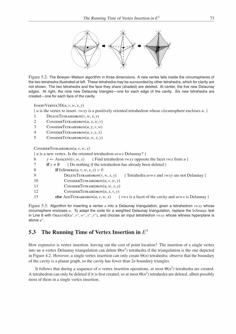
The Running Time of Vertex Insertion in E3 73
Figure 5.2: The Bowyer–Watson algorithm in three dimensions. A new vertex falls inside the circumspheres ofthe two tetrahedra illustrated at left. These tetrahedra may be surrounded by other tetrahedra, which for clarity arenot shown. The two tetrahedra and the face they share (shaded) are deleted. At center, the five new Delaunayedges. At right, the nine new Delaunay triangles—one for each edge of the cavity. Six new tetrahedra arecreated—one for each face of the cavity.
InsertVertex3D(u, v,w, x, y) u is the vertex to insert. vwxy is a positively oriented tetrahedron whose circumsphere encloses u. 1 DeleteTetrahedron(v,w, x, y)2 ConsiderTetrahedron(u, x,w, v)3 ConsiderTetrahedron(u, y, v,w)4 ConsiderTetrahedron(u, v, y, x)5 ConsiderTetrahedron(u,w, x, y)
ConsiderTetrahedron(u, v,w, x) u is a new vertex. Is the oriented tetrahedron uvwx Delaunay? 6 y← Adjacent(v,w, x) Find tetrahedron vwxy opposite the facet vwx from u 7 if y ! ∅ Do nothing if the tetrahedron has already been deleted 8 if InSphere(u, v,w, x, y) > 09 DeleteTetrahedron(v,w, x, y) Tetrahedra uvwx and vwxy are not Delaunay 10 ConsiderTetrahedron(u, v,w, y)11 ConsiderTetrahedron(u,w, x, y)12 ConsiderTetrahedron(u, x, v, y)13 else AddTetrahedron(u, v,w, x) vwx is a facet of the cavity and uvwx is Delaunay
Figure 5.3: Algorithm for inserting a vertex u into a Delaunay triangulation, given a tetrahedron vwxy whosecircumsphere encloses u. To adapt the code for a weighted Delaunay triangulation, replace the InSphere testin Line 8 with Orient4D(u+, v+,w+, x+, y+), and choose an input tetrahedron vwxy whose witness hyperplane isabove u+.
5.3 The Running Time of Vertex Insertion in E3
How expensive is vertex insertion, leaving out the cost of point location? The insertion of a single vertexinto an n-vertex Delaunay triangulation can delete Θ(n2) tetrahedra if the triangulation is the one depictedin Figure 4.2. However, a single vertex insertion can only create Θ(n) tetrahedra: observe that the boundaryof the cavity is a planar graph, so the cavity has fewer than 2n boundary triangles.
It follows that during a sequence of n vertex insertion operations, at most Θ(n2) tetrahedra are created.A tetrahedron can only be deleted if it is first created, so at most Θ(n2) tetrahedra are deleted, albeit possiblymost of them in a single vertex insertion.

74 Jonathan Richard Shewchuk
Randomizing the vertex insertion order does not improve these numbers. For d-dimensional Delaunaytriangulations, the worst-case total number of simplices created and deleted by the incremental insertionalgorithm is in Θ(n⌊d/2⌋+1), and the expected total number of simplices created and deleted by randomincremental insertion is in Θ(n⌈d/2⌉). In the worst case, randomization makes an asymptotic difference onlywhen d is even.
However, a special case that occurs frequently in practice—by all accounts it seems to be the norm—is the circumstance where the Delaunay triangulation has complexity linear, rather than quadratic, in thenumber of vertices, and moreover the intermediate triangulations produced during incremental insertionhave expected linear complexity. For point sets with this property, a random insertion order guarantees thateach vertex insertion will create and delete an expected constant number of tetrahedra, just as it does in theplane, and we shall see that the random incremental insertion algorithm runs in expected O(n log n) time.This running time is often observed in practice, even in higher dimensions. Be forewarned, however, thatthere are point sets for which the final triangulation has linear complexity but the intermediate triangulationshave expected quadratic complexity, thereby slowing down the algorithm dramatically.
Moreover, even for worst-case point sets, randomization helps to support fast point location. Recall thatthe last three steps of the Bowyer–Watson algorithm run in time proportional to the number of tetrahedra theydelete and create, so the running time of the three-dimensional incremental insertion algorithm, excludingpoint location, is in O(n2). With conflict lists and a random insertion order, point location is no moreexpensive than this, so the random incremental insertion algorithm achieves an optimal expected runningtime of O(n2).
5.4 Biased Randomized Insertion Orders
The advantage of inserting vertices in random order is that it guarantees that the expected running time ofpoint location is optimal, and that pathologically slow circumstances like those illustrated in Figure 3.9 areunlikely to happen. But there is a serious disadvantage: random vertex insertions tend to interact poorly withthe memory hierarchy in modern computers, especially virtual memory. Ideally, data structures representingtetrahedra and vertices that are close together geometrically should be close together in memory—a propertycalled spatial locality—for better cache and virtual memory performance.
Amenta, Choi, and Rote [2] show that the permutation of vertices does not need to be uniformly randomfor the running time to be optimal. A biased randomized insertion order (BRIO) is a permutation of thevertices that has strong spatial locality but retains enough randomness to obtain an expected running timein O(n2). Their experiments show that a BRIO greatly improves the efficiency of the memory hierarchy—especially virtual memory.
Their experiments also show that incremental insertion achieves superior running times in practice whenit uses a BRIO but replaces the conflict list with a point location method that simply walks from the pre-viously inserted vertex toward the next inserted vertex; see Section 5.5. Although walking point locationdoes not offer as strong a theoretical guarantee on running time as a conflict list, this incremental insertionalgorithm is perhaps the most attractive in practice, as it combines excellent speed with a simple implemen-tation.
Let n be the number of vertices to triangulate. A BRIO orders the vertices in a sequence of roundsnumbered zero through ⌈log2 n⌉. Each vertex is assigned to the final round, round ⌈log2 n⌉, with probability1/2. The remaining vertices are assigned to the second-last round with probability 1/2, and so on. Each

Point Location by Walking 75
p
Figure 5.4: Walking to the triangle that contains p.
vertex is assign to round zero with probability (1/2)⌈log2 n⌉ ≤ 1/n. The incremental insertion algorithmbegins by inserting the vertices in round zero, then round one, and so on to round ⌈log2 n⌉.
Within any single round, the vertices can be arranged in any order without threatening the worst-caseexpected running time of the algorithm. Hence, we order the vertices within each round to create as muchspatial locality as possible. One way to do this is to insert the vertices in the order they are encountered on aspace-filling curve such as a Hilbert curve or a z-order curve. Another way, which Amenta et al. tested, is tostore the vertices in an octree or k-d tree, refined so each leaf node contains only a few vertices; then orderthe vertices by a traversal of the tree. (Octree traversal is one way to sort vertices along a Hilbert or z-ordercurve.)
The tendency of vertices that are geometrically close together to be close together in the ordering doesnot necessarily guarantee that the data structures associated with them will be close together in memory.Amenta et al. addressed this question experimentally by implementing BRIOs in three different Delaunaytriangulation programs written by three different people, and showing that all three run faster with a BRIOthan with a vertex permutation chosen uniformly at random, especially when the programs run out of mainmemory and have to resort to virtual memory.
Whether you use the traditional random incremental insertion algorithm or a BRIO, you face the problemof bootstrapping the algorithm. The most practical approach is to choose four affinely independent vertices,construct their Delaunay triangulation (a single tetrahedron), create four adjoining ghost tetrahedra, con-struct a conflict list, and insert the remaining vertices in a random order (a uniformly chosen permutation ora BRIO). Even if the four bootstrap vertices are not chosen randomly, it is possible to prove that the expectedasymptotic running time of the algorithm is not compromised.
5.5 Point Location by Walking
By experimentation, Amenta, Choi, and Rote [2] demonstrate that, in conjuction with a BRIO, a simplepoint location method called walking appears to outperform conflict lists in practice, although there is noguarantee of a fast running time. A walking point location algorithm simply traces a straight line throughthe triangulation, visiting tetrahedra that intersect the line as illustrated in Figure 5.4, until it arrives at atetrahedron that contains the new vertex [60]. In conjunction with a vertex permutation chosen uniformly atrandom (rather than a BRIO), walking point location visits many tetrahedra and is very slow. But walking isfast in practice if it follows two guidelines: the vertices should be inserted in an order that has much spatiallocality, such as a BRIO, and each walk should begin at the most recently created tetrahedron. Then thetypical walk visits a small constant number of tetrahdra.
To avoid a long walk between rounds of a BRIO, the vertex order (e.g. the tree traversal or the direction

76 Jonathan Richard Shewchuk
of the space-filling curve) should be reversed on even-numbered rounds, so each round begins near wherethe previous round ends.
Amenta et al. observe that the three-dimensional incremental insertion algorithm with a BRIO and walk-ing point location appears to run in linear time, not counting the initial O(n log n)-time computation of aBRIO. For the point sets in their experiments, this observation holds whether they use a BRIO or a spatialordering (generated by traversing an octree) that has no randomness at all. Randomness is often unnecessaryin practice—frequently, simply sorting the vertices along a space-filling curve will yield excellent speed—but because points sets like that illustrated in Figure 3.9 are common in practice, I recommend choosing aBRIO to prevent the possibility of a pathologically slow running time.
5.6 The Gift-Wrapping Algorithm in E3
The gift-wrapping algorithm described in Section 3.8 requires few new ideas to work in three (or more)dimensions. The algorithm constructs tetrahedra one at a time, and maintains a dictionary of unfinishedfacets. The pseudocode for Finish and GiftWrapCDT can be reused, with triangles replaced by tetrahedra,oriented edges replaced by oriented facets, and circumcircles replaced by circumspheres.
The biggest change is that triangles, not segments, seed the algorithm. But the walls in a PLC arepolygons, and are not always triangles. Recall from Theorem 33 that a CDT of a PLC X induces a two-dimensional CDT of each wall in X. To seed the three-dimensional gift-wrapping algorithm, one can firstcompute the two-dimensional CDT of each wall, then use the triangles in these CDTs to seed the three-dimensional algorithm.
To gift-wrap a Delaunay triangulation, seed the algorithm with one strongly Delaunay triangle. One wayto find one is to choose an arbitrary input point and its nearest neighbor. For the third vertex of the triangle,choose the input point that minimizes the radius of the circle through the three vertices. If the set of inputpoints is generic, the triangle having these three vertices is strongly Delaunay.
If the input (PLC or point set) is not generic, gift-wrapping is in even greater danger in three dimensionsthan in the plane. Whereas the planar gift-wrapping algorithm can handle subsets of four or more cocircularpoints by identifying them and giving them special treatment, no such approach works reliably in threedimensions. Imagine a point set that includes six points lying on a common empty sphere. Suppose thatgift-wrapping inadvertently tetrahedralizes the space around these points so they are the vertices of a hollowcavity shaped like Schonhardt’s polyhedron (from Section 4.5). The algorithm will be unable to fill thecavity. By far the most practical solution is to symbolically perturb the points so that they are generic. Thesame perturbation should also be used to compute the two-dimensional CDTs of the PLC’s walls.
Another difficulty is that the input PLC might not have a CDT, in which case gift-wrapping will fail inone of two ways. One possibility is that the algorithm will fail to finish an unfinished facet, even thoughthere is a vertex in front of that facet, because no vertex in front of that facet is visible from the facet’sinterior. This failure is easy to detect. The second possibility is that the algorithm will finish a facet byconstructing a tetrahedron that is not constrained Delaunay, either because the tetrahedron’s circumsphereencloses a visible vertex, or because the tetrahedron intersects the preexisting simplices wrongly (not in acomplex). An attempt to gift-wrap Schonhardt’s polyhedron brings about the last fate. The algorithm be-comes substantially slower if it tries to detect these failures. Perhaps a better solution is to run the algorithmonly on PLCs that are edge-protected or otherwise known to have CDTs.
A strange property of the CDT is that it is NP-hard to determine whether a PLC has a CDT, if the PLC is

Inserting a Vertex into a Constrained Delaunay Triangulation in E3 77
not generic [59]. However, a polynomial-time algorithm is available for generic PLCs: run the gift-wrappingalgorithm, and check whether it succeeded.
Gift-wrapping takes O(nh) time for a Delaunay triangulation, or O(nmh) time for a CDT, where n is thenumber of input points, m is the total complexity of the input walls, and h is the number of tetrahedra in theCDT; h is usually linear in n, but could be quadratic in the worst case.
5.7 Inserting a Vertex into a Constrained Delaunay Triangulation in E3
Section 3.6 describes how to adapt the Bowyer–Watson vertex insertion algorithm to CDTs in the plane.The same adaptions work for three-dimensional CDTs, but there is a catch: even if a PLC X has a CDT, anaugmented PLC X∪ vmight not have one. This circumstance can be diagnosed after the depth-first searchstep of the Bowyer–Watson algorithm in one of two ways: by the fact that the cavity is not star-shaped, thusone of the newly created tetrahedra has nonpositive orientation, or by the fact that a segment or polygonruns through the interior of the cavity. An implementation can check explicitly for these circumstances, andsignal that the vertex v cannot be inserted.

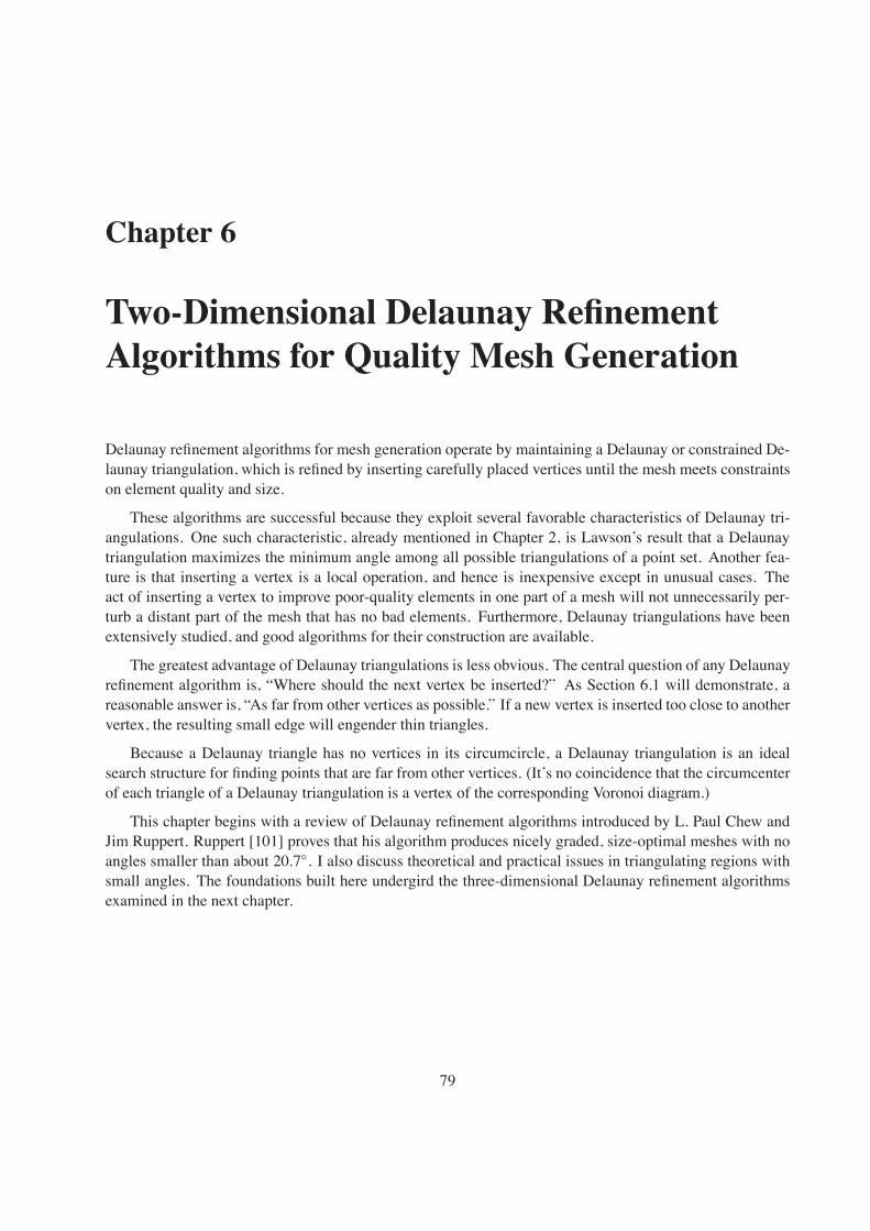
Chapter 6
Two-Dimensional Delaunay RefinementAlgorithms for Quality Mesh Generation
Delaunay refinement algorithms for mesh generation operate by maintaining a Delaunay or constrained De-launay triangulation, which is refined by inserting carefully placed vertices until the mesh meets constraintson element quality and size.
These algorithms are successful because they exploit several favorable characteristics of Delaunay tri-angulations. One such characteristic, already mentioned in Chapter 2, is Lawson’s result that a Delaunaytriangulation maximizes the minimum angle among all possible triangulations of a point set. Another fea-ture is that inserting a vertex is a local operation, and hence is inexpensive except in unusual cases. Theact of inserting a vertex to improve poor-quality elements in one part of a mesh will not unnecessarily per-turb a distant part of the mesh that has no bad elements. Furthermore, Delaunay triangulations have beenextensively studied, and good algorithms for their construction are available.
The greatest advantage of Delaunay triangulations is less obvious. The central question of any Delaunayrefinement algorithm is, “Where should the next vertex be inserted?” As Section 6.1 will demonstrate, areasonable answer is, “As far from other vertices as possible.” If a new vertex is inserted too close to anothervertex, the resulting small edge will engender thin triangles.
Because a Delaunay triangle has no vertices in its circumcircle, a Delaunay triangulation is an idealsearch structure for finding points that are far from other vertices. (It’s no coincidence that the circumcenterof each triangle of a Delaunay triangulation is a vertex of the corresponding Voronoi diagram.)
This chapter begins with a review of Delaunay refinement algorithms introduced by L. Paul Chew andJim Ruppert. Ruppert [101] proves that his algorithm produces nicely graded, size-optimal meshes with noangles smaller than about 20.7. I also discuss theoretical and practical issues in triangulating regions withsmall angles. The foundations built here undergird the three-dimensional Delaunay refinement algorithmsexamined in the next chapter.
79

80 Jonathan Richard Shewchuk
v vt
Figure 6.1: Any triangle whose circumradius-to-shortest edge ratio is larger than some bound B is split byinserting a vertex at its circumcenter. The Delaunay property is maintained, and the triangle is thus eliminated.Every new edge has length at least B times that of shortest edge of the poor triangle.
6.1 The Key Idea Behind Delaunay Refinement
The central operation of Chew’s and Ruppert’s Delaunay refinement algorithms, as well as the three-dimensional algorithms described in the next chapter, is the insertion of a vertex at the circumcenter ofan element of poor quality. The Delaunay property is maintained, using Lawson’s algorithm or the Bowyer–Watson algorithm for the incremental update of Delaunay triangulations. The poor-quality triangle cannotsurvive, because its circumcircle is no longer empty. For brevity, I refer to the act of inserting a vertex ata triangle’s circumcenter as splitting a triangle. The idea dates back at least to the engineering literature ofthe mid-1980s [56]. If poor triangles are split one by one, either all will eventually be eliminated, or thealgorithm will run forever.
The main insight behind all the Delaunay refinement algorithms is that the refinement loop is guaranteedto terminate if the notion of “poor quality” includes only triangles that have a circumradius-to-shortest edgeratio larger than some appropriate bound B. Recall that the only new edges created by the Delaunay insertionof a vertex v are edges connected to v (see Figure 6.1). Because v is the circumcenter of some Delaunaytriangle t, and there were no vertices inside the circumcircle of t before v was inserted, no new edge can beshorter than the circumradius of t. Because t has a circumradius-to-shortest edge ratio larger than B, everynew edge has length at least B times that of the shortest edge of t.
Ruppert’s Delaunay refinement algorithm [102] employs a bound of B =√
2, and Chew’s second Delau-nay refinement algorithm [37] employs a bound of B = 1. Chew’s first Delaunay refinement algorithm [35]splits any triangle whose circumradius is greater than the length of the shortest edge in the entire mesh, thusachieving a bound of B = 1, but forcing all triangles to have uniform size. With these bounds, every newedge created is at least as long as some other edge already in the mesh. Hence, no vertex is ever insertedcloser to another vertex than the length of the shortest edge in the initial triangulation. Delaunay refinementmust eventually terminate, because the augmented triangulation will run out of places to put vertices. Whenit does, all angles are bounded between 20.7 and 138.6 for Ruppert’s algorithm, and between 30 and 120for Chew’s.
Henceforth, a triangle whose circumradius-to-shortest edge ratio is greater than B is said to be skinny.Figure 6.2 provides a different intuition for why all skinny triangles are eventually eliminated by Delaunayrefinement. The new vertices that are inserted into a triangulation (grey dots) are spaced roughly accordingto the length of the shortest nearby edge. Because skinny triangles have relatively large circumradii, their

Chew’s First Delaunay Refinement Algorithm 81
Needle Cap
Figure 6.2: Skinny triangles have circumcircles larger than their shortest edges. Each skinny triangle may beclassified as a needle, whose longest edge is much longer than its shortest edge, or a cap, which has an angleclose to 180. (The classifications are not mutually exclusive.)
circumcircles are inevitably popped. When enough vertices are introduced that the spacing of vertices issomewhat uniform, large empty circumcircles cannot adjoin small edges, and no skinny triangles can remainin the Delaunay triangulation. Fortunately, the spacing of vertices does not need to be so uniform that themesh is poorly graded; this fact is formalized in Section 6.3.4.
These ideas generalize without change to higher dimensions. Imagine a triangulation that has noboundaries—perhaps it has infinite extent, or perhaps it lies in a periodic space that “wraps around” atthe boundaries. Regardless of the dimensionality, Delaunay refinement can eliminate all simplices havinga circumradius-to-shortest edge ratio greater than one, without creating any edge shorter than the shortestedge already present.
Unfortunately, my description of Delaunay refinement thus far has a gaping hole: mesh boundaries havenot been accounted for. The flaw in the procedure described above is that the circumcenter of a poor trianglemight not lie in the mesh at all. Delaunay refinement algorithms, including the two-dimensional algorithmsof Chew and Ruppert and the three-dimensional algorithms described in the next chapter, are distinguishedprimarily by how they handle boundaries. Boundaries complicate mesh generation immensely, and thedifficulty of coping with boundaries increases in higher dimensions.
6.2 Chew’s First Delaunay Refinement Algorithm
Paul Chew has published at least two Delaunay refinement algorithms of great interest. The first, describedhere, produces triangulations of uniform density [35]. The second, which can produce graded meshes [37],is discussed in Section 6.4.
Given a constrained Delaunay triangulation whose shortest edge has length hmin, Chew’s first algorithmsplits any triangle whose circumradius is greater than hmin, and hence creates a uniform mesh. The algorithmnever introduces an edge shorter than hmin, so any two vertices are separated by a distance of at least hmin.The augmented triangulation will eventually run out of places to put vertices, and termination is inevitable.
Of course, the boundaries of the mesh may prevent some skinny triangles from being eliminated. Fig-ure 6.3 illustrates an example in which there is a poor-quality triangle, but no vertex can be placed inside its
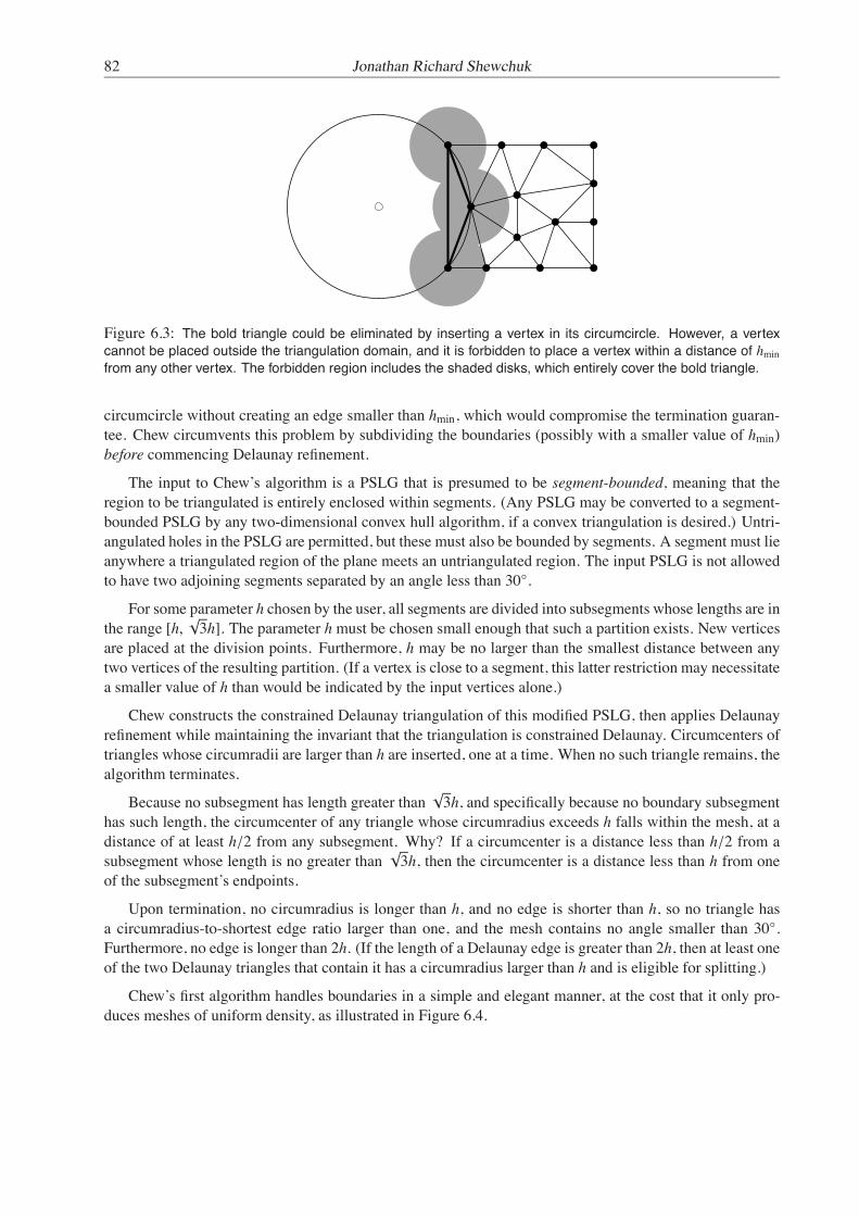
82 Jonathan Richard Shewchuk
Figure 6.3: The bold triangle could be eliminated by inserting a vertex in its circumcircle. However, a vertexcannot be placed outside the triangulation domain, and it is forbidden to place a vertex within a distance of hminfrom any other vertex. The forbidden region includes the shaded disks, which entirely cover the bold triangle.
circumcircle without creating an edge smaller than hmin, which would compromise the termination guaran-tee. Chew circumvents this problem by subdividing the boundaries (possibly with a smaller value of hmin)before commencing Delaunay refinement.
The input to Chew’s algorithm is a PSLG that is presumed to be segment-bounded, meaning that theregion to be triangulated is entirely enclosed within segments. (Any PSLG may be converted to a segment-bounded PSLG by any two-dimensional convex hull algorithm, if a convex triangulation is desired.) Untri-angulated holes in the PSLG are permitted, but these must also be bounded by segments. A segment must lieanywhere a triangulated region of the plane meets an untriangulated region. The input PSLG is not allowedto have two adjoining segments separated by an angle less than 30.
For some parameter h chosen by the user, all segments are divided into subsegments whose lengths are inthe range [h,
√3h]. The parameter h must be chosen small enough that such a partition exists. New vertices
are placed at the division points. Furthermore, h may be no larger than the smallest distance between anytwo vertices of the resulting partition. (If a vertex is close to a segment, this latter restriction may necessitatea smaller value of h than would be indicated by the input vertices alone.)
Chew constructs the constrained Delaunay triangulation of this modified PSLG, then applies Delaunayrefinement while maintaining the invariant that the triangulation is constrained Delaunay. Circumcenters oftriangles whose circumradii are larger than h are inserted, one at a time. When no such triangle remains, thealgorithm terminates.
Because no subsegment has length greater than√
3h, and specifically because no boundary subsegmenthas such length, the circumcenter of any triangle whose circumradius exceeds h falls within the mesh, at adistance of at least h/2 from any subsegment. Why? If a circumcenter is a distance less than h/2 from asubsegment whose length is no greater than
√3h, then the circumcenter is a distance less than h from one
of the subsegment’s endpoints.
Upon termination, no circumradius is longer than h, and no edge is shorter than h, so no triangle hasa circumradius-to-shortest edge ratio larger than one, and the mesh contains no angle smaller than 30.Furthermore, no edge is longer than 2h. (If the length of a Delaunay edge is greater than 2h, then at least oneof the two Delaunay triangles that contain it has a circumradius larger than h and is eligible for splitting.)
Chew’s first algorithm handles boundaries in a simple and elegant manner, at the cost that it only pro-duces meshes of uniform density, as illustrated in Figure 6.4.
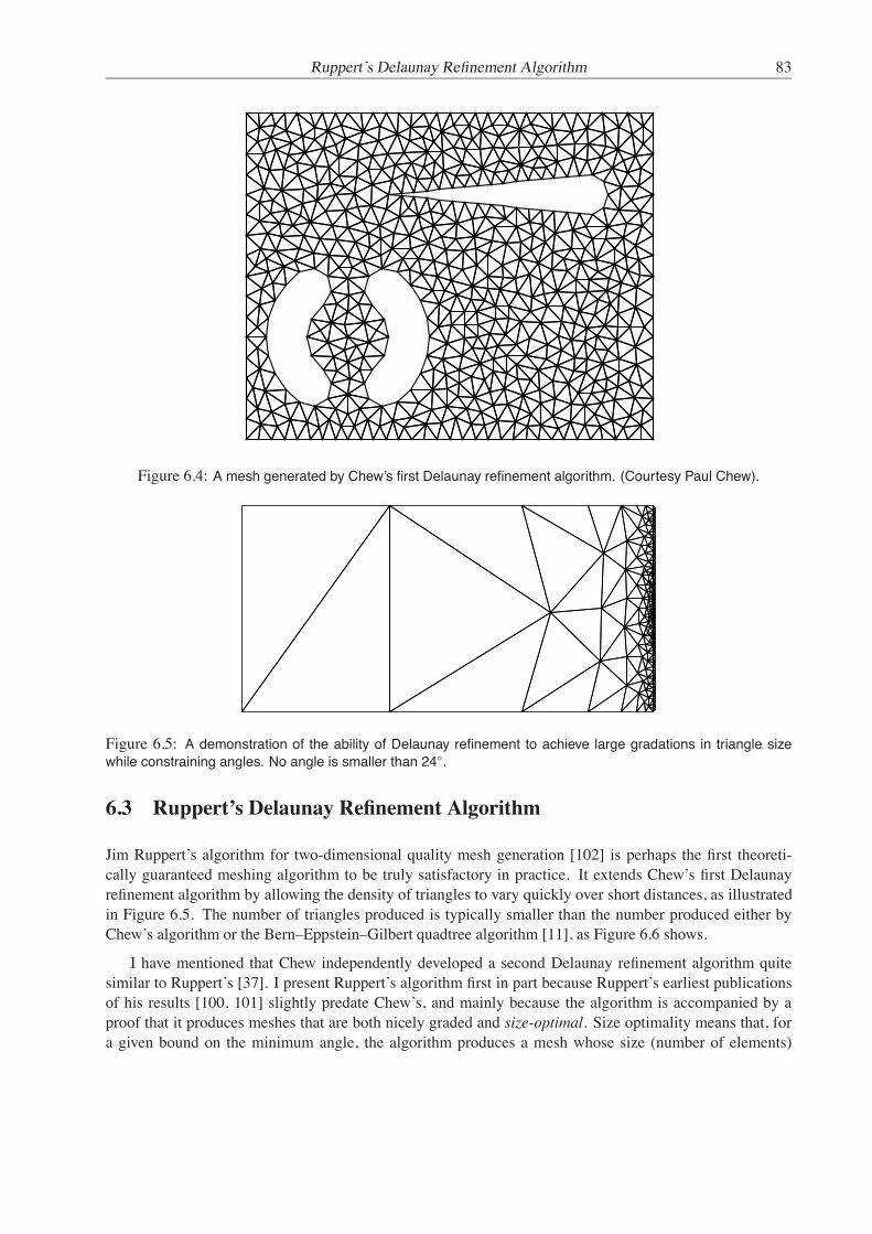
Ruppert’s Delaunay Refinement Algorithm 83
Figure 6.4: A mesh generated by Chew’s first Delaunay refinement algorithm. (Courtesy Paul Chew).
Figure 6.5: A demonstration of the ability of Delaunay refinement to achieve large gradations in triangle sizewhile constraining angles. No angle is smaller than 24.
6.3 Ruppert’s Delaunay Refinement Algorithm
Jim Ruppert’s algorithm for two-dimensional quality mesh generation [102] is perhaps the first theoreti-cally guaranteed meshing algorithm to be truly satisfactory in practice. It extends Chew’s first Delaunayrefinement algorithm by allowing the density of triangles to vary quickly over short distances, as illustratedin Figure 6.5. The number of triangles produced is typically smaller than the number produced either byChew’s algorithm or the Bern–Eppstein–Gilbert quadtree algorithm [11], as Figure 6.6 shows.
I have mentioned that Chew independently developed a second Delaunay refinement algorithm quitesimilar to Ruppert’s [37]. I present Ruppert’s algorithm first in part because Ruppert’s earliest publicationsof his results [100, 101] slightly predate Chew’s, and mainly because the algorithm is accompanied by aproof that it produces meshes that are both nicely graded and size-optimal. Size optimality means that, fora given bound on the minimum angle, the algorithm produces a mesh whose size (number of elements)

84 Jonathan Richard Shewchuk
Figure 6.6: Meshes generated by the Bern–Eppstein–Gilbert quadtree-based algorithm (top), Chew’s first De-launay refinement algorithm (center), and Ruppert’s Delaunay refinement algorithm (bottom). For this polygon,Chew’s second Delaunay refinement algorithm produces nearly the same mesh as Ruppert’s. (The first meshwas produced by the program tripoint, courtesy Scott Mitchell.)
Ruppert’s Delaunay Refinement Algorithm 85
Figure 6.7: Segments are split recursively (while maintaining the constrained Delaunay property) until no sub-segment is encroached.
is at most a constant factor larger than the size of the smallest possible mesh that meets the same anglebound. (The constant depends upon the angle bound, but is independent of the input PSLG. The constantcan be explicitly calculated for any specific angle bound, but it is too large to be useful as a practical bound.)Sections 6.4.2 and 6.4.3 apply Ruppert’s analysis method to Chew’s algorithm, which yields better boundson element quality than Ruppert’s.
6.3.1 Description of the Algorithm
Ruppert’s algorithm is presented here with a few modifications from Ruppert’s original presentation. Themost significant change is that the algorithm here begins with the constrained Delaunay triangulation ofthe segment-bounded PSLG provided as input. In contrast, Ruppert’s presentation begins with a Delaunaytriangulation, and the missing segments are recovered through stitching, described in Section 6.
Ruppert’s algorithm inserts additional vertices (while using Lawson’s algorithm or the Bowyer/Watsonalgorithm to maintain the constrained Delaunay property) until all triangles satisfy the constraints on qualityand size set by the user. Like Chew’s algorithm, Ruppert’s may divide each segment into subsegments—but not as the first step of the algorithm. Instead, the algorithm interleaves segment splitting with trianglesplitting. Initially, each segment comprises one subsegment. Vertex insertion is governed by two rules.
• The diametral circle of a subsegment is the (unique) smallest circle that encloses the subsegment. Asubsegment is said to be encroached if a vertex other than its endpoints lies on or inside its diame-tral circle, and the encroaching vertex is visible from the interior of the subsegment. (Visibility isobstructed only by other segments.) Any encroached subsegment that arises is immediately split intotwo subsegments by inserting a vertex at its midpoint, as illustrated in Figure 6.7. These subsegmentshave smaller diametral circles, and may or may not be encroached themselves; splitting continuesuntil no subsegment is encroached.
• Each skinny triangle (having a circumradius-to-shortest edge ratio greater than some bound B) isnormally split by inserting a vertex at its circumcenter, thus eliminating the triangle. However, if thenew vertex would encroach upon any subsegment, then it is not inserted; instead, all the subsegmentsit would encroach upon are split.
Encroached subsegments are given priority over skinny triangles. The order in which subsegments aresplit, or skinny triangles are split, is arbitrary.
When no encroached subsegments remain, all triangles and edges of the triangulation are Delaunay. Amesh produced by Ruppert’s algorithm is Delaunay, and not just constrained Delaunay.
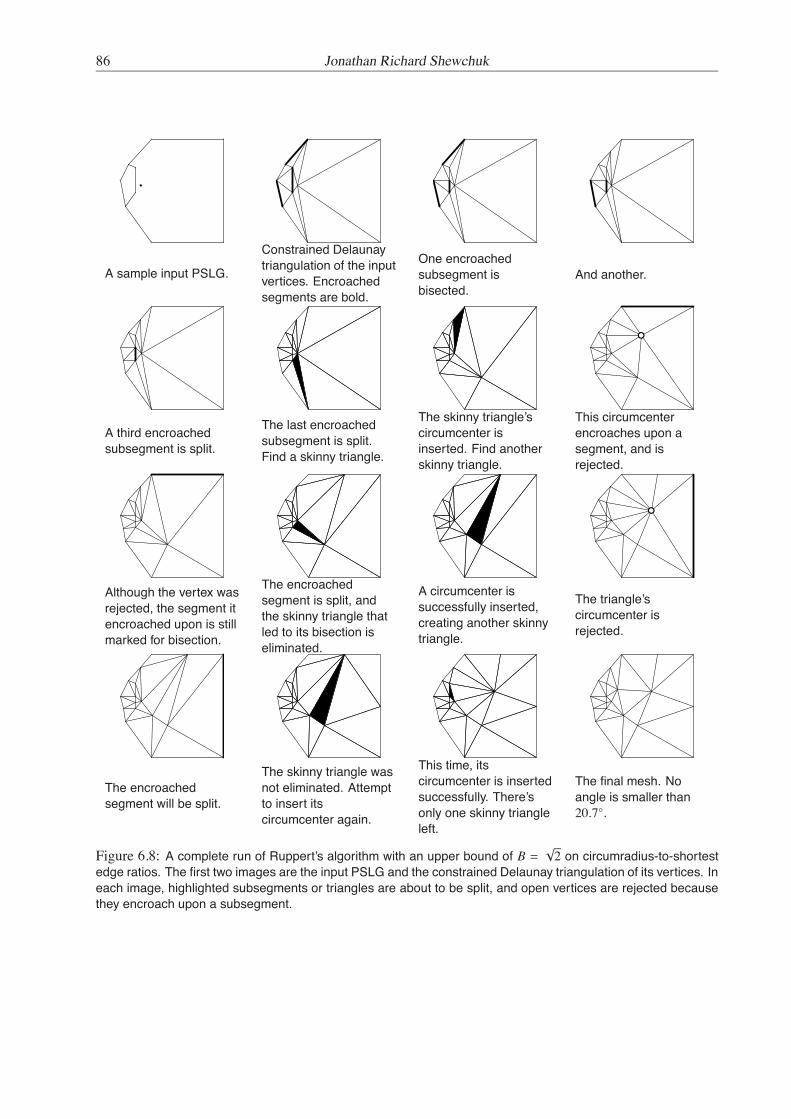
86 Jonathan Richard Shewchuk
A sample input PSLG.
Constrained Delaunaytriangulation of the inputvertices. Encroachedsegments are bold.
One encroachedsubsegment isbisected.
And another.
A third encroachedsubsegment is split.
The last encroachedsubsegment is split.Find a skinny triangle.
The skinny triangle’scircumcenter isinserted. Find anotherskinny triangle.
This circumcenterencroaches upon asegment, and isrejected.
Although the vertex wasrejected, the segment itencroached upon is stillmarked for bisection.
The encroachedsegment is split, andthe skinny triangle thatled to its bisection iseliminated.
A circumcenter issuccessfully inserted,creating another skinnytriangle.
The triangle’scircumcenter isrejected.
The encroachedsegment will be split.
The skinny triangle wasnot eliminated. Attemptto insert itscircumcenter again.
This time, itscircumcenter is insertedsuccessfully. There’sonly one skinny triangleleft.
The final mesh. Noangle is smaller than20.7.
Figure 6.8: A complete run of Ruppert’s algorithm with an upper bound of B =√
2 on circumradius-to-shortestedge ratios. The first two images are the input PSLG and the constrained Delaunay triangulation of its vertices. Ineach image, highlighted subsegments or triangles are about to be split, and open vertices are rejected becausethey encroach upon a subsegment.

Ruppert’s Delaunay Refinement Algorithm 87
c v
st
Figure 6.9: If the circumcenter v of a triangle t lies outside the triangulation, then some subsegment s is en-croached.
Figure 6.8 illustrates the generation of a mesh by Ruppert’s algorithm from start to finish. Severalcharacteristics of the algorithm are worth noting. First, if the circumcenter of a skinny triangle is consideredfor insertion and rejected, it may still be successfully inserted later, after the subsegments it encroaches uponhave been split. On the other hand, the act of splitting those subsegments is sometimes enough to eliminatethe skinny triangle. Second, the smaller features at the left end of the mesh lead to the insertion of somevertices to the right, but the size of the triangles on the right remains larger than the size of the triangles onthe left. The smallest angle in the final mesh is 21.8.
There is a loose end to tie up. What should happen if the circumcenter of a skinny triangle falls outsidethe triangulation? Fortunately, the following lemma shows the question is moot.
Lemma 36. Let T be a segment-bounded Delaunay triangulation. (Hence, any edge of T that belongs toonly one triangle is a subsegment.) Suppose that T has no encroached subsegments. Let v be the circum-center of some triangle t of T . Then v lies in T .
Proof: Suppose for the sake of contradiction that v lies outside T . Let c be the centroid of t; c clearly liesinside T . Because the triangulation is segment-bounded, the line segment cv must cross some subsegments, as Figure 6.9 illustrates. (If there are several such subsegments, let s be the subsegment nearest c.)Because cv is entirely enclosed by the circumcircle of t, the circumcircle must enclose a portion of s; butthe constrained Delaunay property requires that the circumcircle enclose no vertex visible from c, so thecircumcircle cannot enclose the endpoints of s.
Because c and the center of t’s circumcircle lie on opposite sides of s, the portion of the circumcircle thatlies strictly on the same side of s as c (the bold arc in the illustration) is entirely enclosed by the diametralcircle of s. Each vertex of t lies on t’s circumcircle and either is an endpoint of s, or lies on the same sideof s as c. Up to two of the vertices of t may be endpoints of s, but at least one vertex of t must lie strictlyinside the diametral circle of s. But T has no encroached subsegments by assumption; the result follows bycontradiction. "
Lemma 36 offers the best reason why encroached subsegments are given priority over skinny triangles.Because a circumcenter is inserted only when there are no encroached subsegments, one is assured that thecircumcenter will be within the triangulation. The act of splitting encroached subsegments rids the mesh oftriangles whose circumcircles lie outside it. The lemma is also reassuring to applications (like some finitevolume methods) that require all triangle circumcenters to lie within the triangulation.

88 Jonathan Richard Shewchuk
Figure 6.10: The radius of each disk illustrated here is the local feature size of the point at its center.
In addition to being required to satisfy a quality criterion, triangles can also be required to satisfy amaximum size criterion. In a finite element problem, the triangles must be small enough to ensure thatthe finite element solution accurately approximates the true solution of some partial differential equation.Ruppert’s algorithm can allow the user to specify an upper bound on allowable triangle areas or edge lengths,and the bound may be a function of each triangle’s location. Triangles that exceed the local upper boundare split, whether they are skinny or not. So long as the function bounding the sizes of triangles is itselfeverywhere greater than some positive constant, there is no threat to the algorithm’s termination guarantee.
6.3.2 Local Feature Sizes of Planar Straight Line Graphs
The claim that Ruppert’s algorithm produces nicely graded meshes is based on the fact that the spacing ofvertices at any location in the mesh is within a constant factor of the sparsest possible spacing. To formalizethe idea of “sparsest possible spacing,” Ruppert introduces a function called the local feature size, which isdefined over the plane relative to a specific PSLG.
Given a PSLG X, the local feature size lfs(p) at any point p is the radius of the smallest disk centered atp that intersects two nonincident vertices or segments of X. (Two distinct features, each a vertex or segment,are said to be incident if they intersect.) Figure 6.10 illustrates the notion by giving examples of such disksfor a variety of points.
The local feature size of a point is proportional to the sparsest possible spacing of vertices in the neigh-borhood of that point in any triangulation that respects the segments and has no skinny triangles. The func-tion lfs(·) is continuous and has the property that its directional derivatives (where they exist) are boundedin the range [−1, 1]. This property leads to a lower bound (within a constant factor to be derived in Sec-tion 6.3.4) on the rate at which edge lengths grade from small to large as one moves away from a smallfeature. Formally, this is what it means for a mesh to be “nicely graded.”

Ruppert’s Delaunay Refinement Algorithm 89
Lemma 37 (Ruppert [102]). For any PSLG X, and any two points u and v in the plane,
lfs(v) ≤ lfs(u) + |uv|.
Proof: The disk having radius lfs(u) centered at u intersects two nonincident features of X. The disk havingradius lfs(u) + |uv| centered at v contains the prior disk, and thus also intersects the same two features.Hence, the smallest disk centered at v that intersects two nonincident features of X has radius no larger thanlfs(u) + |uv|. "
This lemma generalizes without change to higher dimensions. If the triangulation domain is nonconvexor nonplanar, the lemma can also be generalized to use geodesic distances—lengths of shortest paths thatare constrained to lie within the triangulation domain—instead of straight-line distances. The proof reliesonly on the triangle inequality: if u is within a distance of lfs(u) of each of two nonincident features, then vis within a distance of lfs(u) + |uv| of each of those same two features.
6.3.3 Proof of Termination
Ruppert’s algorithm can eliminate any skinny triangle by inserting a vertex, but new skinny triangles mighttake its place. How can we be sure the process will ever stop? In this section and the next, I present twoproofs of the termination of Ruppert’s algorithm. The first is similar to the proof that Chew’s first algorithmterminates, and is included for its intuitive value, and because it offers the best bound on the lengths of theshortest edges. The second proof, adapted from Ruppert, offers better bounds on the lengths of the longeredges of a graded mesh, and thus shows that the algorithm produces meshes that are nicely graded andsize-optimal. The presentation here uses a flow graph to expose the intuition behind Ruppert’s proof and itsnatural tendency to bound the circumradius-to-shortest edge ratio.
Both proofs require that B ≥√
2, and that any two incident segments (segments that share an endpoint)in the input PSLG are separated by an angle of 60 or greater. (Ruppert asks for angles of at least 90, butthe weaker bound suffices.) For the second proof, these inequalities must be strict.
A mesh vertex is any vertex that has been successfully inserted into the mesh (including the input ver-tices). A rejected vertex is any vertex that is considered for insertion but rejected because it encroaches upona subsegment. With each mesh vertex or rejected vertex v, associate an insertion radius rv, equal to thelength of the shortest edge connected to v immediately after v is introduced into the triangulation. Considerwhat this means in three different cases.
• If v is an input vertex, then rv is the Euclidean distance between v and the nearest input vertex visiblefrom v. See Figure 6.11(a).
• If v is a vertex inserted at the midpoint of an encroached subsegment, then rv is the distance betweenv and the nearest encroaching mesh vertex; see Figure 6.11(b). If there is no encroaching mesh vertex(some triangle’s circumcenter was considered for insertion but rejected as encroaching), then rv is theradius of the diametral circle of the encroached subsegment, and hence the length of each of the twosubsegments thus produced; see Figure 6.11(c).
• If v is a vertex inserted at the circumcenter of a skinny triangle, then rv is the circumradius of thetriangle. See Figure 6.11(d).

90 Jonathan Richard Shewchuk
rvvrv
vrv
vrv
v
(a) (b) (c) (d)
Figure 6.11: The insertion radius rv of a vertex v is the distance to the nearest vertex when v first appears inthe mesh. (a) If v is an input vertex, rv is the distance to the nearest other input vertex. (b) If v is the midpoint ofa subsegment encroached upon by a mesh vertex, rv is the distance to that vertex. (c) If v is the midpoint of asubsegment encroached upon only by a rejected vertex, rv is the radius of the subsegment’s diametral circle. (d)If v is the circumcenter of a skinny triangle, rv is the radius of the circumcircle.
If a vertex is considered for insertion but rejected because of an encroachment, its insertion radius isdefined the same way—as if it had been inserted, even though it is not actually inserted.
Each vertex v, including any rejected vertex, has a parent vertex p(v), unless v is an input vertex. Intu-itively, p(v) is the vertex that is “responsible” for the insertion of v. The parent is defined as follows.
• If v is an input vertex, it has no parent.
• If v is a vertex inserted at the midpoint of an encroached subsegment, then p(v) is the encroachingvertex. (Note that p(v) might be a rejected vertex; a parent need not be a mesh vertex.) If there areseveral encroaching vertices, choose the one nearest v.
• If v is a vertex inserted (or rejected) at the circumcenter of a skinny triangle, then p(v) is the mostrecently inserted endpoint of the shortest edge of that triangle. If both endpoints of the shortest edgeare input vertices, choose one arbitrarily.
Each input vertex is the root of a tree of vertices. However, what is interesting is not each tree as awhole, but the sequence of ancestors of any given vertex, which forms a sort of history of the events leadingto the insertion of that vertex. Figure 6.12 illustrates the parents of all vertices inserted or considered forinsertion during the sample execution of Ruppert’s algorithm in Figure 6.8.
I will use these definitions to show why Ruppert’s algorithm terminates. The key insight is that nodescendant of a mesh vertex has an insertion radius smaller than the vertex’s own insertion radius—unlessthe descendant’s local feature size is even smaller. Therefore, no edge will ever appear that is shorter thanthe smallest feature in the input PSLG. To prove these facts, consider the relationship between the insertionradii of a vertex and its parent.
Lemma 38. Let v be a vertex, and let p = p(v) be its parent, if one exists. Then either rv ≥ lfs(v), orrv ≥ Crp, where
• C = B if v is the circumcenter of a skinny triangle;
• C = 1/√
2 if v is the midpoint of an encroached subsegment and p is the (rejected) circumcenter of askinny triangle;

Ruppert’s Delaunay Refinement Algorithm 91
Figure 6.12: Trees of vertices for the example of Figure 6.8. Arrows are directed from parents to their children.Children include all inserted vertices and one rejected vertex.
• C = 1/(2 cosα) if v and p lie on incident segments separated by an angle of α (with p encroachingupon the subsegment whose midpoint is v), where 45 ≤ α < 90; and
• C = sinα if v and p lie on incident segments separated by an angle of α ≤ 45.
Proof: If v is an input vertex, there is another input vertex a distance of rv from v, so lfs(v) ≤ rv, and thelemma holds.
If v is inserted at the circumcenter of a skinny triangle, then its parent p is the most recently insertedendpoint of the shortest edge of the triangle; see Figure 6.13(a). Hence, the length of the shortest edge ofthe triangle is at least rp. Because the triangle is skinny, its circumradius-to-shortest edge ratio is at least B,so its circumradius is rv ≥ Brp.
If v is inserted at the midpoint of an encroached subsegment s, there are four cases to consider. The firsttwo are all that is needed to prove the termination of Ruppert’s algorithm if no angle smaller than 90 ispresent in the input. The last two cases consider the effects of acute angles.
• If the parent p is an input vertex, or was inserted in a segment not incident to the segment containings, then by definition, lfs(v) ≤ rv.
• If p is a circumcenter that was considered for insertion but rejected because it encroaches upon s,then p lies on or inside the diametral circle of s. Because the mesh is constrained Delaunay, one canshow that the circumcircle centered at p contains neither endpoint of s. Hence, rv ≥ rp/
√2. See
Figure 6.13(b) for an example where the relation is equality.

92 Jonathan Richard Shewchuk
rvrp
p
vrp
rvv
p
2
rp
rv
rv
v
p
a
rvrp
va
p
(a) (b) (c) (d)
Figure 6.13: The relationship between the insertion radii of a child and its parent. (a) When a skinny triangleis split, the child’s insertion radius is at least B times larger than that of its parent. (b) When a subsegment isencroached upon by the circumcenter of a skinny triangle, the child’s insertion radius may be a factor of
√2
smaller than the parent’s, as this worst-case example shows. (c, d) When a subsegment is encroached upon bya vertex in an incident segment, the relationship depends upon the angle α separating the two segments.
• If v and p lie on incident segments separated by an angle α where 45 ≤ α < 90, the vertex a(for “apex”) where the two segments meet obviously cannot lie inside the diametral circle of s; seeFigure 6.13(c). Because s is encroached upon by p, p lies on or inside its diametral circle. To findthe worst-case (smallest) value of rv/rp, imagine that rp and α are fixed; then rv = |vp| is minimizedby making the subsegment s as short as possible, subject to the constraint that p cannot fall outsideits diametral circle. The minimum is achieved when |s| = 2rv. Basic trigonometry shows that |s| ≥rp/ cosα, and therefore rv ≥ rp/(2 cosα).
• If v and p lie on incident segments separated by an angle αwhere α ≤ 45, then rv/rp is minimized notwhen p lies on the diametral circle, but when v is the orthogonal projection of p onto s, as illustratedin Figure 6.13(d). Hence, rv ≥ rp sinα. "
Lemma 38 limits how quickly the insertion radii can decrease through a sequence of descendants of avertex. If vertices with ever-smaller insertion radii cannot be generated, then edges shorter than existingfeatures cannot be introduced, and Delaunay refinement is guaranteed to terminate.
Figure 6.14 expresses this notion as a flow graph. Vertices are divided into three classes: input ver-tices (which are omitted from the figure because they cannot participate in cycles), free vertices insertedat circumcenters of triangles, and segment vertices inserted at midpoints of subsegments. Labeled arrowsindicate how a vertex can cause the insertion of a child whose insertion radius is some factor times that of itsparent. If the graph contains no cycle whose product is less than one, termination is guaranteed. This goalis achieved by choosing B to be at least
√2, and ensuring that the minimum angle between input segments
is at least 60. The following theorem formalizes these ideas.
Theorem 39. Let lfsmin be the shortest distance between two nonincident entities (vertices or segments) ofthe input PSLG1.
1Equivalently, lfsmin = minu lfs(u), where u is chosen from among the input vertices. The proof that both definitions areequivalent is omitted, but it relies on the recognition that if two points lying on nonincident segments are separated by a distance d,then at least one of the endpoints of one of the two segments is separated from the other segment by a distance of d or less. Notethat lfsmin is not a lower bound for lfs(·) over the entire domain; for instance, a segment may have length lfsmin, in which case thelocal feature size at its midpoint is lfsmin/2.

Ruppert’s Delaunay Refinement Algorithm 93
12
12 cos
×
VerticesFree
× B
SegmentVertices
×
Figure 6.14: Flow diagram illustrating the worst-case relation between a vertex’s insertion radius and the insertionradii of the children it begets. If no cycles have a product smaller than one, Ruppert’s Delaunay refinementalgorithm will terminate. Input vertices are omitted from the diagram because they cannot contribute to cycles.
Suppose that any two incident segments are separated by an angle of at least 60, and a triangle isconsidered to be skinny if its circumradius-to-shortest edge ratio is larger than B, where B ≥
√2. Ruppert’s
algorithm will terminate, with no triangulation edge shorter than lfsmin.
Proof: Suppose for the sake of contradiction that the algorithm introduces an edge shorter than lfsmin intothe mesh. Let e be the first such edge introduced. Clearly, the endpoints of e cannot both be input vertices,nor can they lie on nonincident segments. Let v be the most recently inserted endpoint of e.
By assumption, no edge shorter than lfsmin existed before v was inserted. Hence, for any ancestor a of vthat is a mesh vertex, ra ≥ lfsmin. Let p = p(v) be the parent of v, and let g = p(p) be the grandparent of v(if one exists). Consider the following cases.
• If v is the circumcenter of a skinny triangle, then by Lemma 38, rv ≥ Brp ≥√
2rp.
• If v is the midpoint of an encroached subsegment and p is the circumcenter of a skinny triangle, thenby Lemma 38, rv ≥ rp/
√2 ≥ Brg/
√2 ≥ rg. (Recall that p is rejected.)
• If v and p lie on incident segments, then by Lemma 38, rv ≥ rp/(2 cosα). Because α ≥ 60, rv ≥ rp.
In all three cases, rv ≥ ra for some ancestor a of v in the mesh. It follows that rv ≥ lfsmin, contradictingthe assumption that e has length less than lfsmin. It also follows that no edge shorter than lfsmin is everintroduced, so the algorithm must terminate. "
By design, Ruppert’s algorithm terminates only when all triangles in the mesh have a circumradius-to-shortest edge ratio of B or better; hence, at termination, there is no angle smaller than arcsin 1
2B . If B =√
2,the smallest value for which termination is guaranteed, no angle is smaller than 20.7. Section 6.4 describesa way to improve this bound.

94 Jonathan Richard Shewchuk
What about running time? A constrained Delaunay triangulation can be constructed in O(n log n)time [34], where n is the size of the input PSLG. Once the initial triangulation is complete, well-implementedDelaunay refinement algorithms invariably take time linear in the number of additional vertices that are in-serted. Ruppert (personal communication) exhibits a PSLG on which his algorithm takes Θ(h2) time, whereh is the size of the final mesh, but the example is contrived and such pathological examples do not arise inpractice.
6.3.4 Proof of Good Grading and Size-Optimality
Theorem 39 guarantees that no edge of a mesh produced by Ruppert’s algorithm is shorter than lfsmin.This guarantee may be satisfying for a user who desires a uniform mesh, but it is not satisfying for a userwho requires a spatially graded mesh. What follows is a proof that each edge of the output mesh haslength proportional to the local feature sizes of its endpoints. Hence, edge lengths are determined by localconsiderations; features lying outside the disk that defines the local feature size of a point can only weaklyinfluence the lengths of edges that contain that point. Triangle sizes vary quickly over short distances wheresuch variation is desirable to help reduce the number of triangles in the mesh. Readers may skip this sectionwithout affecting their understanding of the rest of the chapter.
Lemma 38 was concerned with the relationship between the insertion radii of a child and its parent.The next lemma is concerned with the relationship between lfs(v)/rv and lfs(p)/rp. For any vertex v, defineDv = lfs(v)/rv. Think of Dv as the one-dimensional density of vertices near v when v is inserted, weightedby the local feature size. One would like this density to be as small as possible. Dv ≤ 1 for any input vertex,but Dv tends to be larger for a vertex inserted late.
Lemma 40. Let v be a vertex with parent p = p(v). Suppose that rv ≥ Crp (following Lemma 38). ThenDv ≤ 1 + Dp/C.
Proof: By Lemma 37, lfs(v) ≤ lfs(p)+ |vp|. By definition, the insertion radius rv is |vp| if p is a mesh vertex,whereas if p is a rejected circumcenter, then rv ≥ |vp|. Hence, we have
lfs(v) ≤ lfs(p) + rv
= Dprp + rv
≤Dp
Crv + rv.
The result follows by dividing both sides by rv. "
Lemma 40 generalizes to any dimension, because it relies only upon Lemma 37. Ruppert’s first mainresult follows.
Lemma 41 (Ruppert [102]). Consider a mesh produced by Ruppert’s algorithm. Suppose the quality boundB is strictly larger than
√2, and the smallest angle between two incident segments in the input PSLG is
strictly greater than 60. There exist fixed constants DT ≥ 1 and DS ≥ 1 such that, for any vertex v inserted(or considered for insertion and rejected) at the circumcenter of a skinny triangle, Dv ≤ DT , and for anyvertex v inserted at the midpoint of an encroached subsegment, Dv ≤ DS . Hence, the insertion radius ofevery vertex has a lower bound proportional to its local feature size.
Ruppert’s Delaunay Refinement Algorithm 95
Proof: Consider any non-input vertex v with parent p = p(v). If p is an input vertex, then Dp = lfs(p)/rp ≤1. Otherwise, assume for the sake of induction that the lemma is true for p, so that Dp ≤ DT if p is acircumcenter, and Dp ≤ DS if p is a midpoint. Hence, Dp ≤ maxDT ,DS .
First, suppose v is inserted or considered for insertion at the circumcenter of a skinny triangle. ByLemma 38, rv ≥ Brp. Thus, by Lemma 40, Dv ≤ 1 + maxDT ,DS /B. It follows that one can prove thatDv ≤ DT if DT is chosen so that
1 +maxDT ,DS
B≤ DT . (6.1)
Second, suppose v is inserted at the midpoint of a subsegment s. If its parent p is an input vertex or lieson a segment not incident to s, then lfs(v) ≤ rv, and the theorem holds. If p is the circumcenter of a skinnytriangle (considered for insertion but rejected because it encroaches upon s), rv ≥ rp/
√2 by Lemma 38, so
by Lemma 40, Dv ≤ 1 +√
2DT .
Alternatively, if p, like v, is a segment vertex, and p and v lie on incident segments, then rv ≥ rp/(2 cosα)by Lemma 38, and thus by Lemma 40, Dv ≤ 1 + 2DS cosα. It follows that one can prove that Dv ≤ DS ifDS is chosen so that
1 +√
2DT ≤ DS , and (6.2)1 + 2DS cosα ≤ DS . (6.3)
If the quality bound B is strictly larger than√
2, Inequalities (6.1) and (6.2) are simultaneously satisfiedby choosing
DT =B + 1
B −√
2, DS =
(1 +√
2)BB −√
2.
If the smallest input angle αmin is strictly greater than 60, Inequalities (6.3) and (6.1) are satisfied bychoosing
DS =1
1 − 2 cosαmin, DT = 1 +
DSB.
One of these choices will dominate, depending on the values of B and αmin. In either case, if B >√
2 andαmin > 60, there are values of DT and DS that satisfy all the inequalities. "
Note that as B approaches√
2 or α approaches 60, DT and DS approach infinity. In practice, thealgorithm is better behaved than the theoretical bound suggests; the vertex density approaches infinity onlyafter B drops below one.
Theorem 42 (Ruppert [102]). For any vertex v of the output mesh, the distance to its nearest neighbor w isat least lfs(v)/(DS + 1).
Proof: Inequality (6.2) indicates that DS > DT , so Lemma 41 shows that lfs(v)/rv ≤ DS for any vertex v. Ifv was added after w, then the distance between the two vertices is rv ≥ lfs(v)/DS , and the theorem holds. Ifw was added after v, apply the lemma to w, yielding
|vw| ≥ rw ≥lfs(w)
DS.
By Lemma 37, lfs(w) + |vw| ≥ lfs(v), so
|vw| ≥lfs(v) − |vw|
DS.

96 Jonathan Richard Shewchuk
Lake Superior PSLG. Triangulated with no minimum angle.
Triangulated with 5 minimum angle. Triangulated with 15 minimum angle.
Triangulated with 25 minimum angle. Triangulated with 34.2 minimum angle.
Figure 6.15: Meshes generated with Ruppert’s algorithm for several different angle bounds. The algorithm doesnot terminate for angle bounds of 34.3 or higher on this PSLG.
It follows that |vw| ≥ lfs(v)/(DS + 1). "
To give a specific example, consider triangulating a PSLG (having no acute input angles) so that no angleof the output mesh is smaller than 15; hence B " 1.93. For this choice of B, DT " 5.66 and DS " 9.01.Hence, the spacing of vertices is at worst about ten times smaller than the local feature size. Away fromboundaries, the spacing of vertices is at worst seven times smaller than the local feature size.
Figure 6.15 illustrates the algorithm’s grading for a variety of angle bounds. Ruppert’s algorithm typi-cally terminates for angle bounds much higher than the theoretically guaranteed 20.7, and typically exhibitsmuch better vertex spacing than the provable worst-case bounds imply.
Ruppert [102] uses Theorem 42 to prove the size optimality of the meshes his algorithm generates, andhis result has been improved by Mitchell [83]. Mitchell’s theorem is stated below, but the lengthy proof isomitted.

Chew’s Second Delaunay Refinement Algorithm 97
Theorem 43 (Mitchell [83]). Let lfsT (p) be the local feature size at p with respect to a triangulation T(treating T as a PSLG), whereas lfs(p) remains the local feature size at p with respect to the input PSLG.Suppose a triangulation T with smallest angle θ has the property that there is some constant k1 ≥ 1 suchthat for every point p, k1lfsT (p) ≥ lfs(p). Then the cardinality (number of triangles) of T is less than k2times the cardinality of any other triangulation of the input PSLG with smallest angle θ, where k2 ∈ O(k2
1/θ)."
Theorem 42 can be used to show that the precondition of Theorem 43 is satisfied by meshes generatedby Ruppert’s algorithm (with k1 ∝ DS ). Hence, the cardinality of a mesh generated by Ruppert’s algorithmis within a constant factor of the cardinality of the best possible mesh satisfying the angle bound. However,the constant factor hidden in Mitchell’s theorem is much too large to be a meaningful guarantee in practice.
6.4 Chew’s Second Delaunay Refinement Algorithm
Compared to Ruppert’s algorithm, Chew’s second Delaunay refinement algorithm [37] offers an improvedguarantee of good grading in theory, and splits fewer subsegments in practice. This section shows that thealgorithm exhibits good grading and size optimality for angle bounds of up to 26.5 (compared with 20.7for Ruppert’s algorithm).
Chew’s paper also discusses triangular meshing of curved surfaces in three dimensions, but I considerthe algorithm only in its planar context.
6.4.1 Description of the Algorithm
Chew’s second Delaunay refinement algorithm begins with the constrained Delaunay triangulation of asegment-bounded PSLG, and eliminates skinny triangles through Delaunay refinement, but Chew does notuse diametral circles to determine if subsegments are encroached. Instead, it may arise that a skinny trianglet cannot be split because t and its circumcenter c lie on opposite sides of a subsegment s. (Lemma 36 doesnot apply to Chew’s algorithm, so c may even lie outside the triangulation.) Although Chew does not usethe word, let us say that s is encroached when this circumstance occurs.
Because s is a subsegment, inserting a vertex at c will not remove t from the mesh. Instead, c is rejected,and all free vertices that lie inside the diametral circle of s and are visible from the midpoint of s are deletedfrom the triangulation. (Input vertices and segment vertices are not deleted.) Then, a new vertex is insertedat the midpoint of s. The constrained Delaunay property is maintained throughout all vertex deletions andinsertions. Figure 6.16 illustrates a subsegment split in Chew’s algorithm.
If several subsegments lie between t and c, only the subsegment nearest t is split. If no subsegment liesbetween t and c, but c lies precisely on a subsegment, then that subsegment is considered encroached andsplit at its midpoint.
Chew’s second algorithm produces a mesh that is not guaranteed to be Delaunay (only constrainedDelaunay). For the few applications that require truly Delaunay triangles, Ruppert’s algorithm is preferable.For the majority of applications, however, Chew has two advantages. First, some subsegment splits areavoided that would otherwise have occurred, so the final mesh may have fewer triangles. Consider twocontrasting examples. In Figure 6.6 (bottom), the segments are so short that few are ever encroached, soRuppert and Chew generate virtually the same mesh. In Figure 6.17, the segments are long compared totheir local feature sizes, and Chew produces many fewer triangles.

98 Jonathan Richard Shewchuk
t
c
Figure 6.16: At left, a skinny triangle and its circumcenter lie on opposite sides of a subsegment. At right, allvertices in the subsegment’s diametral circle have been deleted, and a new vertex has been inserted at thesubsegment’s midpoint.
Figure 6.17: A PSLG, a 559-triangle mesh produced by Ruppert’s algorithm, and a 423-triangle mesh producedby Chew’s second algorithm. No angle in either mesh is smaller than 25.
The second advantage is that when a subsegment is split by a vertex v with parent p, a better bound canbe found for the ratio between rv and rp than Lemma 38’s bound. This improvement leads to better boundson the minimum angle, the edge lengths, and the mesh cardinality.
6.4.2 Proof of Termination
If no input angle is less than 60, Chew’s algorithm terminates for any bound on circumradius-to-shortestedge ratio B such that B ≥
√5/2 " 1.12. Therefore, the smallest angle can be bounded by up to
arcsin(1/√
5) " 26.56.
By the reasoning of Lemma 36, if a triangle and its circumcenter lie on opposite sides of a subsegment,or if the circumcenter lies on the subsegment, then some vertex of the triangle (other than the subsegment’sendpoints) lies on or inside the subsegment’s diametral circle. Hence, Chew’s algorithm never splits asubsegment that Ruppert’s algorithm would not split. It follows that the inequalities in Lemma 38 are astrue for Chew’s algorithm as they are for Ruppert’s algorithm. However, Chew will often decline to split asubsegment that Ruppert would split, and thus splits fewer subsegments overall. A consequence is that the

Chew’s Second Delaunay Refinement Algorithm 99
0 0rv
ru
rvv
u
rv rv rv rv
rv rv
rv
v(a) (b)
Figure 6.18: (a) The case where exactly one vertex is in the semicircle. (b) The case where more than onevertex is in the semicircle.
relationship between the insertion radii of a subsegment midpoint and its parent can be tightened.
Lemma 44. Let θ = arcsin 12B be the angle bound below which a triangle is considered skinny. Let s be a
subsegment that is encroached because some skinny triangle t and its circumcenter c lie on opposite sides ofs (or c lies on s). Let v be the vertex inserted at the midpoint of s. Then one of the following four statementsis true. (Only the fourth differs from Lemma 38.)
• rv ≥ lfs(v);
• rv ≥ rp/(2 cosα), where p is a vertex that encroaches upon s and lies in a segment separated by anangle of α ≥ 45 from the segment containing s;
• rv ≥ rp sinα, where p is as above, with α ≤ 45; or
• there is some vertex p (which is deleted from inside the diametral circle of s or lies precisely on thediametral circle) such that rv ≥ rp cos θ.
Proof: Chew’s algorithm deletes all free vertices inside the diametral circle of s that are visible from v. Ifany vertex remains visible from v inside the diametral circle, it is an input vertex or a segment vertex. Definethe parent p of v to be the closest such vertex. If p is an input vertex or lies on a segment not incident tothe segment that contains s, then lfs(v) ≤ rv and the lemma holds. If p lies on an incident segment, thenrv ≥ rp/(2 cosα) for α ≥ 45 or rv ≥ rp cos θ for α ≤ 45 as in Lemma 38.
Otherwise, no vertex inside the diametral circle of s is visible after the deletions, so rv is equal to theradius of the diametral circle. This is the reason why Chew’s algorithm deletes the vertices: when v isinserted, the nearest visible vertices are the subsegment endpoints, and no short edge appears.
Mentally jump back in time to just before the vertex deletions. Assume without loss of generality that tlies above s, with c below. Following Lemma 36, at least one vertex of t lies on or inside the upper half ofthe diametral circle of s. There are two cases, depending on the total number of vertices on or inside thissemicircle.
If the upper semicircle encloses only one vertex u visible from v, then t is the triangle whose verticesare u and the endpoints of s. Because t is skinny, u must lie in the shaded region of Figure 6.18(a). Theinsertion radius ru cannot be greater than the distance from u to the nearest endpoint of s, so rv ≥ ru cos θ.(For a fixed rv, ru is maximized when u lies at the apex of the isosceles triangle whose base is s and whosebase angles are θ.) Define the parent of v to be u.
If the upper semicircle encloses more than one vertex visible from v, consider Figure 6.18(b), in whichthe shaded region represents points within a distance of rv from an endpoint of s. If some vertex u lies in
100 Jonathan Richard Shewchuk
the shaded region, then ru ≤ rv; define the parent of v to be u. If no vertex lies in the shaded region, thenthere are at least two vertices visible from v in the white region of the upper semicircle. Let u be the mostrecently inserted of these vertices. The vertex u is at a distance of at most rv from any other vertex in thewhite region, so ru ≤ rv; define the parent of v to be u. "
Lemma 44 extends the definition of parent to accommodate the new type of encroachment defined inChew’s algorithm. When a subsegment s is encroached, the parent p of its newly inserted midpoint v isdefined to be a vertex on or inside the diametral circle of s, just as in Ruppert’s algorithm.
Chew’s algorithm can be shown to terminate in the same manner as Ruppert’s. Do the differencesbetween Chew’s and Ruppert’s algorithms invalidate any of the assumptions used in Theorem 39 to provetermination? The most important difference is that vertices may be deleted from the mesh. When a vertex isdeleted from a constrained Delaunay triangulation, no surviving vertex finds itself adjoining a shorter edgethan the shortest edge it adjoined before the deletion. (This fact follows because a constrained Delaunaytriangulation connects every vertex to its nearest visible neighbor.) Hence, each vertex’s insertion radius stillserves as a lower bound on the lengths of all edges that connect the vertex to vertices older than itself.
If vertices can be deleted, are we certain that the algorithm will run out of places to put new vertices?Observe that vertex deletions only occur when a subsegment is split, and vertices are never deleted fromsegments. Theorem 39 sets a lower bound on the length of each subsegment, so only a finite number ofsubsegment splits can occur. After the last subsegment split, no more vertex deletions occur, and eventuallythere will be no space left for new vertices. Therefore, Theorem 39 and Lemma 41 hold for Chew’s algorithmas well as Ruppert’s.
The consequence of the bound proven by Lemma 44 is illustrated in the flow graph of Figure 6.19. Recallthat termination is guaranteed if no cycle has a product less than one. Hence, a condition of termination isthat B cos θ ≥ 1. As θ = arcsin 1
2B , the best bound that satisfies this criterion is B =√
5/2 " 1.12, whichcorresponds to an angle bound of arcsin(1/
√5) " 26.56.
6.4.3 Proof of Good Grading and Size Optimality
The main point of this section is to demonstrate that Chew’s algorithm offers better theoretical guaranteesabout triangle quality, edge lengths, and good grading than Ruppert’s. (We should not forget, though, thatit is Ruppert’s analysis technique that allows us to draw this conclusion.) Whereas Ruppert only guaranteesgood grading and size optimality for angle bounds less than about 20.7, Chew can make these promisesfor angle bounds less than about 26.5, and offer better bounds on edge lengths for the angle bounds whereRuppert’s guarantees do hold. However, the differences are not as pronounced in practice as in theory.Readers whose interests are purely practical may skip this section without affecting their understanding ofthe rest of the chapter.
Let’s compare Chew’s algorithm.
Lemma 45. Consider a mesh produced by Chew’s algorithm. Suppose the quality bound B is strictly largerthan
√5/2, and the smallest angle between two incident segments in the input PSLG is strictly greater than
60. There exist fixed constants DT ≥ 1 and DS ≥ 1 such that, for any vertex v inserted at the circumcenterof a skinny triangle, Dv ≤ DT , and for any vertex v inserted at the midpoint of an encroached subsegment,Dv ≤ DS .

Chew’s Second Delaunay Refinement Algorithm 101
× cos 0
12 cos
Vertices
Free
× B
Vertices
×
Segment
Figure 6.19: Flow diagram for Chew’s algorithm.
Proof: Essentially the same as the proof of Lemma 41, except that Lemma 44 makes it possible to replaceInequality (6.2) with
DS ≥ 1 +DT
cos θ
≥ 1 +2BDT√4B2 − 1
(6.4)
If the quality bound B is strictly larger than√
5/2, Inequalities (6.1) and (6.4) are simultaneously satis-fied by choosing
DT =
&
1 + 1B
' √4B2 − 1
√4B2 − 1 − 2
, DS =
√4B2 − 1 + 2B√
4B2 − 1 − 2.
DT and DS must also satisfy Inequality (6.3), so larger values of DT and DS may be needed, as inLemma 41. However, If B >
√5/2 and αmin > 60, there are values of DT and DS that satisfy all the
inequalities. "
Theorem 42, which bounds the edge lengths of the mesh, applies to Chew’s algorithm as well as Rup-pert’s, but the values of DT and DS are different. As in Section 6.3.4, consider triangulating a PSLG (freeof acute angles) so that no angle of the output mesh is smaller than 15. Then DT " 3.27, and DS " 4.39,compared to the corresponding values of 5.66 and 9.01 for Ruppert’s algorithm. Hence, the spacing of ver-tices is at worst a little more than five times the local feature size, and a little more than four times the localfeature size away from segments.
Because the worst-case number of triangles is proportional to the square of DS , Chew’s algorithm issize-optimal with a constant of optimality almost four times better than Ruppert’s algorithm. However,worst-case behavior is never seen in practice, and the observed difference between the two algorithms is lessdramatic.

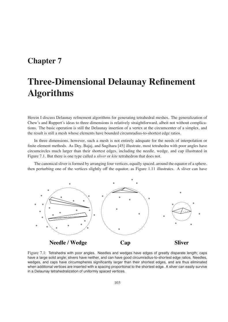
Chapter 7
Three-Dimensional Delaunay RefinementAlgorithms
Herein I discuss Delaunay refinement algorithms for generating tetrahedral meshes. The generalization ofChew’s and Ruppert’s ideas to three dimensions is relatively straightforward, albeit not without complica-tions. The basic operation is still the Delaunay insertion of a vertex at the circumcenter of a simplex, andthe result is still a mesh whose elements have bounded circumradius-to-shortest edge ratios.
In three dimensions, however, such a mesh is not entirely adequate for the needs of interpolation orfinite element methods. As Dey, Bajaj, and Sugihara [45] illustrate, most tetrahedra with poor angles havecircumcircles much larger than their shortest edges, including the needle, wedge, and cap illustrated inFigure 7.1. But there is one type called a sliver or kite tetrahedron that does not.
The canonical sliver is formed by arranging four vertices, equally spaced, around the equator of a sphere,then perturbing one of the vertices slightly off the equator, as Figure 1.11 illustrates. A sliver can have
Needle / Wedge Cap SliverFigure 7.1: Tetrahedra with poor angles. Needles and wedges have edges of greatly disparate length; capshave a large solid angle; slivers have neither, and can have good circumradius-to-shortest edge ratios. Needles,wedges, and caps have circumspheres significantly larger than their shortest edges, and are thus eliminatedwhen additional vertices are inserted with a spacing proportional to the shortest edge. A sliver can easily survivein a Delaunay tetrahedralization of uniformly spaced vertices.
103

104 Jonathan Richard Shewchuk
an admirable circumradius-to-shortest edge ratio (as low as 1√2!) yet be considered awful by most other
measures, because its volume and its shortest altitude can be arbitrarily close to zero, and its dihedral anglescan be arbitrarily close to 0 and 180. Slivers have no two-dimensional analogue; any triangle with a smallcircumradius-to-shortest edge ratio is considered “well-shaped” by the usual standards of finite elementmethods and interpolation.
Slivers often survive Delaunay-based tetrahedral mesh generation methods because their small circum-radii minimize the likelihood of vertices being inserted in their circumspheres (as Figure 7.1 illustrates). Aperfectly flat sliver whose edge lengths are lfsmin about the equator and
√2lfsmin across the diagonals is
guaranteed to survive any Delaunay refinement method that does not introduce edges smaller than lfsmin,because every point in the interior of its circumsphere is a distance less than lfsmin from one of its vertices;no vertex can be inserted inside the sphere.
Despite slivers, Delaunay refinement methods are valuable for generating three-dimensional meshes.Slivers having good circumradius-to-shortest edge ratios typically arise in small numbers in practice. AsSection 7.3 will demonstrate, the worst slivers can often be removed by Delaunay refinement, even if there isno theoretical guarantee. Meshes with bounds on the circumradius-to-shortest edge ratios of their tetrahedraare an excellent starting point for mesh smoothing and optimization methods that remove slivers and improvethe quality of an existing mesh. The most notable of these is the sliver exudation algorithm of Cheng, Dey,Edelsbrunner, Facello, and Teng [30], which is based on weighted Delaunay triangulations. Even if sliversare not removed, the Voronoi dual of a tetrahedralization with bounded circumradius-to-shortest edge ratioshas nicely rounded cells, and is sometimes ideal for use in the control volume method [81].
In this chapter, I present a three-dimensional generalization of Ruppert’s algorithm that generates tetra-hedralizations whose tetrahedra have circumradius-to-shortest edge ratios no greater than the bound B =√
2 " 1.41. If B is relaxed to be greater than two, then good grading can also be proven. Size-optimality,however, cannot be proven.

Definitions 105
(a) (b)
Figure 7.2: (a) Any facet of a PLC may contain holes, slits, and vertices. (b) When a PLC is tetrahedralized,each facet of the PLC is partitioned into triangular subfacets, which respect the holes, slits, and vertices.
F S
Figure 7.3: The orthogonal projections of points and sets of points onto facets and segments.
7.1 Definitions
Tetrahedral mesh generation necessarily divides each facet of a PLC, like that depicted in Figure 7.2(a),into triangular faces, as illustrated in Figure 7.2(b). Just as the triangulation edges that comprise a segmentare called subsegments, the triangular faces that comprise a facet are called subfacets. The bold edges inFigure 7.2(b) are subsegments; other edges are not. All of the triangular faces visible in Figure 7.2(b) aresubfacets, but most of the faces in the interior of the tetrahedralization are not.
Frequently in this chapter, I use the notion of the orthogonal projection of a geometric entity onto a lineor plane. Given a facet or subfacet F and a point p, the orthogonal projection projF(p) of p onto F is thepoint that is coplanar with F and lies in the line that passes through p orthogonally to F, as illustrated inFigure 7.3. The projection exists whether or not it falls in F.
Similarly, the orthogonal projection projS (p) of p onto a segment or subsegment S is the point that iscollinear with S and lies in the plane through p orthogonal to S .
Sets of points, as well as points, may be projected. If F and G are facets, then projF(G) is the setprojF(p) : p ∈ G.
7.2 A Three-Dimensional Delaunay Refinement Algorithm
In this section, I describe a three-dimensional Delaunay refinement algorithm that produces well-gradedtetrahedral meshes satisfying any circumradius-to-shortest edge ratio bound greater than two. Miller, Tal-

106 Jonathan Richard Shewchuk
mor, Teng, Walkington, and Wang [82] have developed a related algorithm that does not use Delaunayrefinement.
7.2.1 Description of the Algorithm
Three-dimensional Delaunay refinement takes a facet-bounded PLC as its input. Tetrahedralized and unte-trahedralized regions of space must be separated by facets so that, in the final mesh, any triangular face notshared by two tetrahedra is a subfacet.
Many approaches to tetrahedral mesh generation permanently triangulate the input facets as a separatestep prior to tetrahedralizing the interior of a region. The problem with this approach is that these indepen-dent facet triangulations may not be collectively ideal for forming a good tetrahedralization. For instance, afeature that lies near a facet (but not necessarily in the plane of the facet) may necessitate the use of smallersubfacets near that feature. The present algorithm uses another approach, wherein facet triangulations arerefined in conjunction with the tetrahedralization. The tetrahedralization process is not beholden to poordecisions made earlier.
Any vertex inserted into a segment or facet during Delaunay refinement remains there permanently.However, keep in mind that the edges that partition a facet into subfacets are not permanent, are not treatedlike subsegments, and are subject to flipping (within the facet) according to the Delaunay criterion.
The algorithm’s first step is to construct a Delaunay tetrahedralization of the input vertices. Some inputsegments and facets might be missing (or partly missing) from this mesh. As in two dimensions, the tetrahe-dralization is refined by inserting additional vertices into the mesh, using an incremental Delaunay tetrahe-dralization algorithm such as the Bowyer–Watson algorithm [20, 128] or three-dimensional flipping [66, 96],until all segments and facets are recovered and all constraints on tetrahedron quality and size are met. Vertexinsertion is governed by three rules.
• The diametral sphere of a subsegment is the (unique) smallest sphere that contains the subsegment.A subsegment is encroached if a vertex other than its endpoints lies inside or on its diametral sphere.(This definition of encroachment is slightly stronger than that used by Ruppert’s algorithm, to ensurethat all unencroached subsegments are strongly Delaunay. This makes it possible to form a CDT, andalso strengthens an upcoming result called the Projection Lemma.) A subsegment may be encroachedwhether or not it actually appears as an edge of the tetrahedralization. If a subsegment is missingfrom the tetrahedralization, it is not strongly Delaunay and thus must be encroached. Any encroachedsubsegment that arises is immediately split into two subsegments by inserting a vertex at its midpoint.See Figure 7.4(a).
• The equatorial sphere of a triangular subfacet is the (unique) smallest sphere that passes through thethree vertices of the subfacet. (The equator of an equatorial sphere is the unique circle that passesthrough the same three vertices.) A subfacet is encroached if a non-coplanar vertex lies inside or onits equatorial sphere. If a subfacet is missing from the tetrahedralization, and it is not covered by otherfaces that share the same circumcircle, then it is encroached. (The question of what subfacets shouldnot be missing from the tetrahedralization will be considered shortly.) Each encroached subfacetis normally split by inserting a vertex at its circumcenter; see Figure 7.4(b). However, if the newvertex would encroach upon any subsegment, it is not inserted; instead, all the subsegments it wouldencroach upon are split.

A Three-Dimensional Delaunay Refinement Algorithm 107
(a) (b) (c)
Figure 7.4: Three operations for three-dimensional Delaunay refinement. (a) Splitting an encroached subseg-ment. Dotted arcs indicate where diametral spheres intersect faces. The original subsegment is encroachedbecause there is a vertex in its diametral sphere. In this example, the two subsegments created by bisectingthe original subsegment are not encroached. (b) Splitting an encroached subfacet. The triangular faces shownare subfacets of a larger facet, with tetrahedra (not shown) atop them. A vertex in the equatorial sphere of asubfacet causes a vertex to be inserted at its circumcenter. In this example, all equatorial spheres (included thetwo illustrated) are empty after the split. (c) Splitting a skinny tetrahedron. A vertex is inserted at its circumcenter.
• A tetrahedron is said to be skinny if its circumradius-to-shortest edge ratio is larger than some boundB. (By this definition, not all slivers are considered skinny.) Each skinny tetrahedron is normally splitby inserting a vertex at its circumcenter, thus eliminating the tetrahedron; see Figure 7.4(c). However,if the new vertex would encroach upon any subsegment or subfacet, then it is not inserted; instead,all the subsegments it would encroach upon are split. If the skinny tetrahedron is not eliminated as aresult, then all the subfacets its circumcenter would encroach upon are split. (A subtle point is that, ifthe tetrahedron is eliminated by subsegment splitting, the algorithm should not split any subfacets thatappear during subsegment splitting, or the bounds proven later will not be valid. Lazy programmersbeware.)
Encroached subsegments are given priority over encroached subfacets, which have priority over skinnytetrahedra. These encroachment rules are intended to recover missing segments and facets, and to ensurethat all vertex insertions are valid. Because all facets are segment-bounded, Lemma 36 shows that if thereare no encroached subsegments, then each subfacet circumcenter lies in the containing facet. One can alsoshow (with a similar proof) that if there are no encroached subfacets, then each tetrahedron circumcenterlies in the mesh.
Missing subsegments are recovered by stitching, described in Section 6. If a subsegment is missing froma Delaunay triangulation, then the subsegment is not strongly Delaunay, so there must be a vertex (other than

108 Jonathan Richard Shewchuk
Facet Triangulation
MeshPLC
Figure 7.5: The top illustrations depict a rectangular facet and its triangulation. The bottom illustrations depictthe facet’s position as an interior boundary of a PLC, and its progress as it is recovered. Most of the vertices andtetrahedra of the mesh are omitted for clarity. The facet triangulation and the tetrahedralization are maintainedseparately. Shaded triangular subfacets in the facet triangulation (top center) are missing from the tetrahedral-ization (bottom center). The bold dashed line (bottom center) represents a tetrahedralization edge that passesthrough the facet. A missing subfacet is recovered by inserting a vertex at its circumcenter (top right and bottomright). The vertex is independently inserted into both the triangulation and the tetrahedralization.
its endpoints) on or inside its diametral circle. This observation is important because it unifies the theoreticaltreatment of missing subsegments and encroached subsegments that are not missing.
When no encroached subsegment remains, missing facets are recovered in an analogous manner. Themain complication is that if a facet is missing from the mesh, it is difficult to say what its subfacets are.With segments there is no such problem; if a segment is missing from the mesh, and a vertex is inserted atits midpoint, one knows unambiguously where the two resulting subsegments are. But how may we identifysubfacets that do not yet exist?
The solution is straightforward. For each facet, it is necessary to maintain a two-dimensional Delau-nay triangulation of its vertices, independently from the tetrahedralization in which we hope its subfacetswill eventually appear. By comparing the triangles of a facet’s triangulation against the faces of the tetra-

A Three-Dimensional Delaunay Refinement Algorithm 109
Figure 7.6: If a tetrahedron is Delaunay, the circumcircle of each of its faces is empty, because each face’scircumcircle is a cross-section of the tetrahedron’s circumsphere.
hedralization, one can identify subfacets that need to be recovered. For each triangular subfacet in a facettriangulation, look for a matching face in the tetrahedralization; if the latter is missing, insert a vertex atthe circumcenter of the subfacet (subject to rejection if subsegments are encroached), as illustrated in Fig-ure 7.5. The new vertex is independently inserted into both the facet triangulation and the tetrahedralization.Similarly, the midpoint of an encroached subsegment is independently inserted into the tetrahedralizationand into each facet triangulation that contains the subsegment.
In essence, Ruppert’s algorithm (and the present algorithm) uses the same procedure to recover seg-ments. However, the process of forming a one-dimensional triangulation is so simple that it passes unno-ticed.
Which vertices of the tetrahedralization need to be considered in a facet triangulation? It is a fact, albeitsomewhat nonintuitive, that if a facet appears in a Delaunay tetrahedralization as a union of faces, then thetriangulation of the facet is determined solely by the vertices of the tetrahedralization that lie in the planeof the facet. If a vertex lies near a facet, but is not coplanar with the facet, it may cause a subfacet tobe missing (as in Figure 7.5, bottom center), but it cannot otherwise affect the shape of the triangulation.Why? Suppose a subfacet of a facet appears in the tetrahedralization. Then the subfacet must be a face ofa Delaunay tetrahedron. The subfacet’s circumcircle is empty, because its circumcircle is a cross-section ofthe tetrahedron’s empty circumsphere, as illustrated in Figure 7.6. Therefore, if a facet appears as a unionof faces in a Delaunay tetrahedralization, then those faces form a two-dimensional Delaunay triangulationof the facet. Because the Delaunay triangulation is unique (except in nondegenerate cases), vertices that donot lie in the plane of the facet have no effect on how the facet is triangulated.
Furthermore, because each facet is segment-bounded, and segments are recovered (in the tetrahedral-ization) before facets, each facet triangulation can safely ignore vertices that lie outside the facet (coplanarthough they may be). A triangulation need only take into account the segments and vertices in the facet. Therequirements set forth in Section 4.5.1 ensure that all of the vertices and segments of a facet must be explic-itly identified in the input PLC. The only additional vertices to be considered are those that were inserted insegments to help recover those segments and other facets. The algorithm maintains a list of the vertices oneach segment, ready to be called upon when a facet triangulation is initially formed.
Unfortunately, if a facet’s Delaunay triangulation is not unique because of cocircularity degeneracies,then the facet might be represented in the tetrahedralization by faces that do not match the independent facettriangulation, as Figure 7.7 illustrates. (If exact arithmetic is not used, nearly-degenerate cases may teamup with floating-point roundoff error to make this circumstance more common.) An implementation must

110 Jonathan Richard Shewchuk
Figure 7.7: A facet triangulation and a tetrahedralization may disagree due to cocircular vertices. This occurrenceshould be diagnosed and fixed as shown here.
detect these cases and correct the triangulation so that it matches the tetrahedralization. (It is not alwayspossible to force the tetrahedralization to match the triangulation.)
To appreciate the advantages of this facet recovery method, compare it with the most popular method [61,129, 99]. In many tetrahedral mesh generators, facets are inserted by identifying points where the edges ofthe tetrahedralization intersect a missing facet, and inserting vertices at these points. The perils of so doingare illustrated in Figure 7.8. In the illustration, a vertex is inserted where a tetrahedralization edge (bolddashed line) intersects the facet. Unfortunately, the edge intersects the facet near one of the boundingsegments of the facet, and the new vertex creates a feature that may be arbitrarily small. Afterward, theonly alternatives are to refine the tetrahedra near the new vertex to a small size, or to move or remove thevertex. Some mesh generators cope with this problem by smoothing the vertices on each facet after the facetis competely inserted.
The encroachment-based facet recovery method does not insert such vertices at all. A vertex consideredfor insertion too close to a segment is rejected, and a subsegment is split instead. This would not necessarilybe true if edge-facet intersections were considered for insertion, because such an intersection may be neara vertex lying on the segment, and thus fail to encroach upon any subsegments. Subfacet circumcenters arebetter choices because they are far from the nearest vertices, and cannot create a new small feature withoutencroaching upon a subsegment.
Of course, an even better idea is to form a conforming CDT of the input PLC as soon as all the segmentshave been recovered by stitching, thereby recovering the facets without inserting additional vertices. Thismeasure helps to mitigate (but not eliminate) the unwanted effects of small exterior feature sizes. For thepurposes of analysis, however, it is instructive to consider the variant of the algorithm that uses unconstrainedDelaunay triangulations.
When no encroached subsegment or subfacet remains, every input segment and facet is represented by aunion of edges or faces of the mesh. The first time the mesh reaches this state, all exterior tetrahedra (lying

A Three-Dimensional Delaunay Refinement Algorithm 111
Figure 7.8: One may recover a missing facet by inserting vertices at the intersections of the facet with edgesof the tetrahedralization, but this method might create arbitrarily small features by placing vertices close to seg-ments.
in the convex hull of the input vertices, but outside the region enclosed by the facet-bounded PLC) shouldbe removed prior to splitting any skinny tetrahedra. This measure prevents the problems that can arise ifsuperfluous skinny tetrahedra are split, such as overrefinement and failure to terminate because of exteriorsmall angles and spurious small angles formed between the PLC and its convex hull.
One further amendment to the algorithm is necessary to obtain the best possible bound on the circum-radius-to-shortest edge ratios of the tetrahedra. It would be nice to prove, in the manner of Lemma 38, thatwhenever an encroached subfacet is split at its circumcenter, the insertion radius of the newly inserted vertexis no worse than
√2 times smaller than the insertion radius of its parent. Unfortunately, this is not true for
the algorithm described above.
Consider the two examples of Figure 7.9. If a subfacet that contains its own circumcenter is encroached,then the distance between the encroaching vertex and the nearest vertex of the subfacet is no more than√
2 times the circumradius of the subfacet. This distance is maximized if the encroaching vertex lies at apole of the equatorial sphere (where the poles are the two points of the sphere furthest from its equator), asillustrated in Figure 7.9(a). However, if a subfacet that does not contain its own circumcenter is encroached,the distance is maximized if the encroaching vertex lies on the equator, equidistant from the two vertices ofthe longest edge of the subfacet, as in Figure 7.9(b). Even if the encroaching vertex is well away from theequator, its distance from the nearest vertex of the subfacet can still be larger than
√2 times the radius of
the equatorial sphere. (I have confirmed through my implementation that such cases do arise in practice.)
Rather than settle for a looser guarantee on quality, one can make a small change to the algorithm thatwill yield a
√2 bound. When several encroached subfacets exist, they should not be split in arbitrary order.
If a vertex p encroaches upon a subfacet f of a facet F, but the projected point projF(p) does not lie in f ,then splitting f is not the best choice. One can show (with the following lemma) that there is some othersubfacet g of F that is encroached upon by p and contains projF(p). (The lemma assumes that there areno encroached subsegments in the mesh, as they have priority.) A better bound is achieved if the algorithm

112 Jonathan Richard Shewchuk
r
r
2r
(a) (b)
Figure 7.9: The relationship between the insertion radii of the circumcenter of an encroached subfacet and theencroaching vertex. Crosses identify the location of an encroaching vertex having maximum distance from thenearest subfacet vertex. (a) If the encroached subfacet contains its own circumcenter, the encroaching vertexis no further from the nearest vertex of the subfacet than
√2 times the circumradius of the subfacet. (b) If the
encroached subfacet does not contain its own circumcenter, the encroaching vertex may be further away.
s
F
S
Fprojpf
c
sphere of s
outsideinside
(p)
ofsphereequatorial
f
diametral
F
f
c geof
sphereequatorial
f
equatorialsphere
gof
E
p
(a) (b)
Figure 7.10: Two properties of encroached Delaunay subfacets. (a) If a vertex p encroaches upon a Delaunaysubfacet f of a facet F, but its projection into the plane containing F lies outside F, then p encroaches upon somesubsegment s of F as well. (b) If a vertex p encroaches upon a subfacet f of a Delaunay triangulated facet F,but does not encroach upon any subsegment of F, then p encroaches upon the subfacet(s) g of F that containsprojF(p).
splits g first and delays the splitting of f indefinitely.
Lemma 46 (Projection Lemma). Let f be a subfacet of the Delaunay triangulated facet F. Suppose that fis encroached upon by some vertex p, but p does not encroach upon any subsegment of F. Then projF(p)lies in the facet F, and p encroaches upon a subfacet of F that contains projF(p).
Proof: First, I prove that projF(p) lies in F, using similar reasoning to that employed in Lemma 36. Supposefor the sake of contradiction that projF(p) lies outside the facet F. Let c be the centroid of f ; c clearly liesinside F. Because all facets are segment-bounded, the line segment connecting c to projF(p) must intersectsome subsegment s in the boundary of F. Let S be the plane that contains s and is orthogonal to F, asillustrated in Figure 7.10(a).
Because f is a Delaunay subfacet of F, its circumcircle (in the plane containing F) encloses no vertex
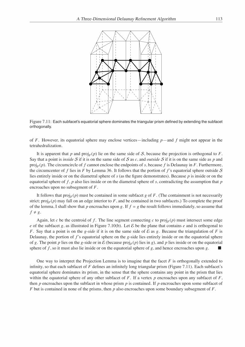
A Three-Dimensional Delaunay Refinement Algorithm 113
Figure 7.11: Each subfacet’s equatorial sphere dominates the triangular prism defined by extending the subfacetorthogonally.
of F. However, its equatorial sphere may enclose vertices—including p—and f might not appear in thetetrahedralization.
It is apparent that p and projF(p) lie on the same side of S, because the projection is orthogonal to F.Say that a point is inside S if it is on the same side of S as c, and outside S if it is on the same side as p andprojF(p). The circumcircle of f cannot enclose the endpoints of s, because f is Delaunay in F. Furthermore,the circumcenter of f lies in F by Lemma 36. It follows that the portion of f ’s equatorial sphere outside Slies entirely inside or on the diametral sphere of s (as the figure demonstrates). Because p is inside or on theequatorial sphere of f , p also lies inside or on the diametral sphere of s, contradicting the assumption that pencroaches upon no subsegment of F.
It follows that projF(p) must be contained in some subfacet g of F. (The containment is not necessarilystrict; projF(p) may fall on an edge interior to F, and be contained in two subfacets.) To complete the proofof the lemma, I shall show that p encroaches upon g. If f = g the result follows immediately, so assume thatf ! g.
Again, let c be the centroid of f . The line segment connecting c to projF(p) must intersect some edgee of the subfacet g, as illustrated in Figure 7.10(b). Let E be the plane that contains e and is orthogonal toF. Say that a point is on the g-side if it is on the same side of E as g. Because the triangulation of F isDelaunay, the portion of f ’s equatorial sphere on the g-side lies entirely inside or on the equatorial sphereof g. The point p lies on the g-side or in E (because projF(p) lies in g), and p lies inside or on the equatorialsphere of f , so it must also lie inside or on the equatorial sphere of g, and hence encroaches upon g. "
One way to interpret the Projection Lemma is to imagine that the facet F is orthogonally extended toinfinity, so that each subfacet of F defines an infinitely long triangular prism (Figure 7.11). Each subfacet’sequatorial sphere dominates its prism, in the sense that the sphere contains any point in the prism that lieswithin the equatorial sphere of any other subfacet of F. If a vertex p encroaches upon any subfacet of F,then p encroaches upon the subfacet in whose prism p is contained. If p encroaches upon some subfacet ofF but is contained in none of the prisms, then p also encroaches upon some boundary subsegment of F.
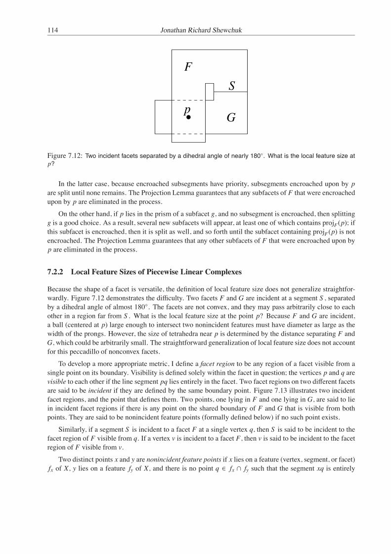
114 Jonathan Richard Shewchuk
S
G
F
p
Figure 7.12: Two incident facets separated by a dihedral angle of nearly 180. What is the local feature size atp?
In the latter case, because encroached subsegments have priority, subsegments encroached upon by pare split until none remains. The Projection Lemma guarantees that any subfacets of F that were encroachedupon by p are eliminated in the process.
On the other hand, if p lies in the prism of a subfacet g, and no subsegment is encroached, then splittingg is a good choice. As a result, several new subfacets will appear, at least one of which contains projF(p); ifthis subfacet is encroached, then it is split as well, and so forth until the subfacet containing projF(p) is notencroached. The Projection Lemma guarantees that any other subfacets of F that were encroached upon byp are eliminated in the process.
7.2.2 Local Feature Sizes of Piecewise Linear Complexes
Because the shape of a facet is versatile, the definition of local feature size does not generalize straightfor-wardly. Figure 7.12 demonstrates the difficulty. Two facets F and G are incident at a segment S , separatedby a dihedral angle of almost 180. The facets are not convex, and they may pass arbitrarily close to eachother in a region far from S . What is the local feature size at the point p? Because F and G are incident,a ball (centered at p) large enough to intersect two nonincident features must have diameter as large as thewidth of the prongs. However, the size of tetrahedra near p is determined by the distance separating F andG, which could be arbitrarily small. The straightforward generalization of local feature size does not accountfor this peccadillo of nonconvex facets.
To develop a more appropriate metric, I define a facet region to be any region of a facet visible from asingle point on its boundary. Visibility is defined solely within the facet in question; the vertices p and q arevisible to each other if the line segment pq lies entirely in the facet. Two facet regions on two different facetsare said to be incident if they are defined by the same boundary point. Figure 7.13 illustrates two incidentfacet regions, and the point that defines them. Two points, one lying in F and one lying in G, are said to liein incident facet regions if there is any point on the shared boundary of F and G that is visible from bothpoints. They are said to be nonincident feature points (formally defined below) if no such point exists.
Similarly, if a segment S is incident to a facet F at a single vertex q, then S is said to be incident to thefacet region of F visible from q. If a vertex v is incident to a facet F, then v is said to be incident to the facetregion of F visible from v.
Two distinct points x and y are nonincident feature points if x lies on a feature (vertex, segment, or facet)fx of X, y lies on a feature fy of X, and there is no point q ∈ fx ∩ fy such that the segment xq is entirely

A Three-Dimensional Delaunay Refinement Algorithm 115
G
F
Figure 7.13: Shaded areas are two incident facet regions. Both regions are visible from the indicated point.
F
G
Svp
Figure 7.14: Two incident facets separated by a dihedral angle of nearly 180. The definition of local feature sizeshould not approach zero near v, but it is nonetheless difficult to mesh the region between F and G near v.
contained in fx and the segment yq is entirely contained in fy. (Note that q may be x or y.) If such a pointq does exist, then x and y lie in incident vertices, segments, or facet regions of X. However, each pointmay lie in several features simultaneously; so even if x and y lie in incident facet regions, they may still benonincident feature points (if they lie in nonincident segments, for instance).
Given a piecewise linear complex X, I define the local feature size lfs(p) at a point p to be the radius ofthe smallest ball centered at p that intersects a pair of nonincident feature points.
Unfortunately, careful specification of which portions of facets are incident doesn’t solve all the prob-lems attributable to nonconvex facets. Figure 7.14 demonstrates another difficulty. Again, two facets F andG are incident at a segment S , separated by a dihedral angle slightly less than 180. One endpoint v of S is areflex vertex of F. The incident facet regions defined by the vertex v have the same problem we encounteredin Figure 7.12: the local feature size at point p may be much larger than the distance between facets F andG at point p.
In this case, however, the problem is unavoidable. Suppose one chooses a definition of local feature sizethat reflects the distance between F and G at p. As p moves toward v, lfs(p) approaches zero, suggestingthat infinitesimally small tetrahedra are needed to mesh the region near v. Intuitively and practically, a usefuldefinition of local feature size must have a positive lower bound. Therefore, lfs(p) cannot be proportional tothe distance between F and G at p.

116 Jonathan Richard Shewchuk
The mismatch between the definition of local feature size proposed here and the small distance betweenF and G at p reflects a fundamental difficulty in meshing the facets of Figure 7.14—a difficulty that isnot present in Figure 7.12. In Figure 7.14, it is not possible to mesh the region between F and G at vwithout resorting to poorly shaped tetrahedra. The facets of Figure 7.12 can be meshed entirely with well-shaped tetrahedra. The three-dimensional Delaunay refinement algorithm discussed here outlaws inputs likeFigure 7.14, at least for the purposes of analysis.
Lemma 37, which states that lfs(v) ≤ lfs(u) + |uv| for any two points u and v, applies to this definition oflocal feature size just as it applies in two dimensions. The only prerequisite for the correctness of Lemma 37,besides the triangle inequality, is that there be a consistent definition of which pairs of points are nonincidentfeature points.
7.2.3 Proof of Termination
The proof of termination for three-dimensional Delaunay refinement is similar to that of Ruppert’s two-dimensional algorithm. Assume that in the input PLC, any two incident segments are separated by an angleof 60 or greater. If a segment meets a facet at one vertex v, and the orthogonal projection of the segmentonto the facet intersects the interior of the facet region defined by v, then the angle separating the segmentfrom the facet must be no less than arccos 1
2√
2" 69.3. If the projection of the segment does not intersect
the interior of the facet, the Projection Lemma implies that no vertex on the segment can encroach upon anysubfacet of the facet without also encroaching upon a boundary segment of the facet, so the 69.3 separationangle is unnecessary. However, there still must be a 60 separation between the segment and the segmentsincident on v that bound the facet.
The condition for two incident facets is more complicated. If both facets are convex and meet at asegment, then it is sufficient for the facets to be separated by a dihedral angle of 90 or greater. In general,the two facets must satisfy the following projection condition.
For any point p where two facets F and G meet, let visp(F) be the facet region of F visible from p,and define visp(G) likewise. By definition, visp(F) and visp(G) are incident facet regions. No point of theorthogonal projection of visp(F) onto G may intersect the interior of visp(G). (Here, “interior” is definedto exclude all boundaries, including isolated slits and input vertices in the interior of the facet.) Formally,for any point p on F ∩ G, the projection condition requires that projG(visp(F)) ∩ interior(visp(G)) = ∅, orequivalently, that projF(visp(G)) ∩ interior(visp(F)) = ∅.
The payoff of this restriction is that, by Lemma 46, no vertex in visp(F) may encroach upon a subfacetcontained entirely in visp(G) without also encroaching upon a subsegment of G or a subfacet of G notentirely in visp(G). The converse is also true. The purpose of this restriction is so that no vertex can splita subfacet in a facet region incident to a facet region containing that vertex. Otherwise, subfacets might besplit to arbitrarily small sizes through mutual encroachment in regions arbitrarily close to p.
The projection condition just defined is always satisfied by two facets separated by a dihedral angle ofexactly 90. It is also satisfied by facets separated by a dihedral angle greater than 90 if the facets meet eachother only at segments whose endpoints are not reflex vertices of either facet. (Recall Figure 7.14, whichdepicts two facets that are separated by a dihedral angle greater than 90 but fail the projection conditionbecause v is a reflex vertex of F.)
The following lemma extends Lemma 38 to three dimensions. It is true if the algorithm never splits anyencroached subfacet f that does not contain the projection proj f (p) of the encroaching vertex p. (Even more
A Three-Dimensional Delaunay Refinement Algorithm 117
liberally, an implementation can easily measure the insertion radii of the parent p and its potential progeny,and may split f if the latter is no less than 1√
2times the former.)
The insertion radius is defined as before: rv is the length of the shortest edge incident to v immediatelyafter v is inserted. The parent of a vertex is defined as before, with the following amendments. If v is thecircumcenter of a skinny tetrahedron, its parent p(v) is the most recently inserted endpoint of the shortestedge of that tetrahedron. If v is the circumcenter of an encroached subfacet, its parent is the encroachingvertex closest to v (whether that vertex is inserted or rejected).
Lemma 47. Let v be a vertex, and let p = p(v) be its parent, if one exists. Then either rv ≥ lfs(v), orrv ≥ Crp, where
• C = B if v is the circumcenter of a skinny tetrahedron;
• C = 1√2
if v is the midpoint of an encroached subsegment or the circumcenter of an encroachedsubfacet;
• C = 12 cosα if v and p lie on incident segments separated by an angle of α, or if v lies in the interior of
a facet incident to a segment containing p at an angle α, where 45 ≤ α < 90.
Proof: If v is an input vertex, the circumcenter of a tetrahedron (Figure 7.15(a)), or the midpoint of anencroached subsegment, then it may be treated exactly as in Lemma 38. One case from that lemma is worthbriefly revisiting to show that nothing essential has changed.
If v is inserted at the midpoint of an encroached subsegment s, and its parent p = p(v) is a circumcenter(of a tetrahedron or subfacet) that was considered for insertion but rejected because it encroaches upons, then p lies inside or on the diametral sphere of s. Because the tetrahedralization/facet triangulationis Delaunay, the circumsphere/circumcircle centered at p encloses no vertices, and in particular does notenclose the endpoints of s. Hence, rp ≤
√2rv; see Figure 7.15(b) for an example where the relation
is equality. Note that the change from circles (in the two-dimensional analysis) to spheres makes littledifference. Perhaps the clearest way to see this is to observe that if one takes a two-dimensional cross-section that passes through s and p, the cross-section is indistinguishable from the two-dimensional case.(The same argument can be made for the case where p and v lie on incident segments.)
Only the circumstance where v is the circumcenter of an encroached subfacet f remains. Let F be thefacet that contains f . There are four cases to consider.
• If the parent p is an input vertex, or if v and p are nonincident feature points, then lfs(v) ≤ rv.
• If p is a tetrahedron circumcenter that was considered for insertion but rejected because it encroachesupon f , then p lies strictly inside the equatorial sphere of f . Because the tetrahedralization is Delau-nay, the circumsphere centered at p contains no vertices, including the vertices of f . The subfacet fcontains proj f (p); otherwise, the algorithm would choose a different encroached subfacet to split first.The height of p above proj f (p) is no greater than rv, and the distance between proj f (p) and the nearestvertex of f is no greater than rv (because proj f (p) lies in f ), so rp ≤
√2rv. See Figure 7.15(c) for an
example where the relation is equality.
• If p was inserted on a segment that is incident to F at one vertex a, separated by an angle of α ≥ 45(Figure 7.15(d)), the shared vertex a cannot lie inside the equatorial sphere of f because the facet Fis Delaunay triangulated. (This is true even if f does not appear in the tetrahedralization.) Because

118 Jonathan Richard Shewchuk
v >
rv
rp
r rpBp
v
2r= v
rv
p
v
rp
rp
(a) (b)
2r= v
rvf
p
v
rp
rp
2
rvrp
rv
p
fva
(c) (d)
Figure 7.15: The relationship between the insertion radii of a child and its parent. (a) When a skinny tetrahedronis split, the child’s insertion radius is at least B times larger than that of its parent. (b) When a subsegment isencroached upon by a circumcenter, the child’s insertion radius may be a factor of
√2 smaller than its parent’s.
(c) When a subfacet is encroached upon by the circumcenter of a skinny tetrahedron, and the subfacet containsthe orthogonal projection of the encroaching circumcenter, the child’s insertion radius may be a factor of
√2
smaller than its parent’s. (d) When a subfacet is encroached upon by the midpoint of a subsegment, and thecorresponding facet and segment are incident at one vertex, the analysis differs little from the case of two incidentsegments.
the segment and facet are separated by an angle of α, the angle ∠pav is at least α. Because f isencroached upon by p, p lies inside its equatorial sphere. (If f is not present in the tetrahedralization,p might lie on its equatorial sphere in a degenerate case.) Analogously to the case of two incidentsegments (see Lemma 38), if α ≥ 45, then rv
rpis minimized when the radius of the equatorial sphere
is rv = |vp|, and p lies on the sphere. (If the equatorial sphere were any smaller, it could not containp.) Therefore, rv ≥
rp2 cosα . "
Lemma 47 provides the information one needs to ensure that Delaunay refinement will terminate. Aswith the two dimensional algorithms, the key is to prevent any vertex from begetting a sequence of descen-dants with ever-smaller insertion radii.

A Three-Dimensional Delaunay Refinement Algorithm 119
12
12
×
Subfacet
TetrahedronCircumcenters
×2
×
MidpointsSubsegment
Circumcenters
Figure 7.16: Flow diagram illustrating the worst-case relation between a vertex’s insertion radius and the insertionradii of the children it begets. If no cycle has a product smaller than one, the three dimensional Delaunayrefinement algorithm will terminate.
Figure 7.16 depicts a flow graph corresponding to Lemma 47. Mesh vertices are divided into fourclasses: input vertices (which cannot contribute to cycles), segment vertices (inserted into segments), facetvertices (inserted into facet interiors), and free vertices (inserted at circumcenters of tetrahedra). As we haveseen, free vertices can father facet vertices whose insertion radii are smaller by a factor of
√2, and these facet
vertices in turn can father segment vertices whose insertion radii are smaller by another factor of√
2. Hence,to avoid spiralling into the abyss, it is important that segment vertices can only father free vertices whoseinsertion radii are at least twice as large. This constraint fixes the best guaranteed circumradius-to-shortestedge ratio at B = 2.
The need to prevent diminishing cycles also engenders the requirement that incident segments be sepa-rated by angles of 60 or more, just as it did in the two-dimensional case. A segment incident to a facet mustbe separated by an angle of at least arccos 1
2√
2" 69.3 so that if a vertex on the segment encroaches upon
a subfacet of the facet, the child that results will have an insertion radius at least√
2 larger than that of itsparent. (Recall from Lemma 47 that rv ≥
rp2 cosα .)
Theorem 48. Let lfsmin be the shortest distance between two nonincident feature points of the input PLC.Suppose that any two incident segments are separated by an angle of at least 60, any two incident facetregions satisfy the projection condition, and any segment incident to a facet region at one vertex is separatedfrom it by an angle of at least arccos 1
2√
2or satisfies the projection condition.
Suppose a tetrahedron is considered to be skinny if its circumradius-to-shortest edge ratio is larger thanB, where B ≥ 2. The three-dimensional Delaunay refinement algorithm described above will terminate, withno tetrahedralization edge shorter than lfsmin.

120 Jonathan Richard Shewchuk
Proof: Suppose for the sake of contradiction that the algorithm introduces one or more edges shorter thanlfsmin into the mesh. Let e be the first such edge introduced. Clearly, the endpoints of e cannot both be inputvertices, nor can they lie on nonincident feature points. Let v be the most recently inserted endpoint of e.
By assumption, no edge shorter than lfsmin existed before v was inserted. Hence, for any ancestor a of vthat is a mesh vertex, ra ≥ lfsmin. Let p = p(v) be the parent of v, let g = p(p) be the grandparent of v (if oneexists), and let h = p(g) be the great-grandparent of v (if one exists). Because of the projection condition, vand p cannot lie in incident facet regions. Consider the following cases.
• If v is the circumcenter of a skinny tetrahedron, then by Lemma 47, rv ≥ Brp ≥ 2rp.
• If v is the midpoint of an encroached subsegment or the circumcenter of an encroached subfacet, andp is the circumcenter of a skinny tetrahedron, then by Lemma 47, rv ≥ 1√
2rp ≥ B√
2rg ≥
√2rg.
• If v is the midpoint of an encroached subsegment, p is the circumcenter of an encroached subfacet,and g is the circumcenter of a skinny tetrahedron, then by Lemma 47, rv ≥ 1√
2rp ≥ 1
2 rg ≥ B2 rh ≥ rh.
• If v and p lie on incident segments, then by Lemma 47, rv ≥rp
2 cosα . Because α ≥ 60, rv ≥ rp.
• If v is the circumcenter of an encroached subfacet and p lies on a segment incident (at a single vertex)to the facet containing v, then by Lemma 47, rv ≥
rp2 cosα . Because α ≥ arccos 1
2√
2, rv ≥
√2rp.
• If v is the midpoint of an encroached subsegment, p is the (rejected) circumcenter of an encroachedsubfacet, and g lies on a segment incident (at a single vertex) to the facet containing p, then byLemma 47, rv ≥ 1√
2rp ≥ 1
2√
2 cosαrg. Because α ≥ arccos 1
2√
2, rv ≥ rg.
• If v is the midpoint of an encroached subsegment, and p has been inserted on a nonincident segmentor facet region, then by the definition of parent, pv is the shortest edge introduced by the insertion ofv. Because p and v lie on nonincident entities, p and v are separated by a distance of at least lfsmin,contradicting the assumption that e has length less than lfsmin.
In the first six cases, rp ≥ ra for some mesh vertex a that is an ancestor of p. It follows that rp ≥ lfsmin,contradicting the assumption that e has length less than lfsmin. Because no edge shorter than lfsmin is everintroduced, the algorithm must terminate. "
7.2.4 Proof of Good Grading
As with the two-dimensional algorithm, a stronger termination proof is possible, showing that each edgeof the output mesh has length proportional to the local feature sizes of its endpoints, and thus guaranteeingnicely graded meshes. The proof makes use of Lemma 40, which generalizes unchanged to three or moredimensions. Recall that the lemma states that if rv ≥ Crp for some vertex v with parent p, then theirlfs-weighted vertex densities are related by the formula Dv ≤ 1 + Dp
C , where Dv =lfs(v)
rvand Dp =
lfs(p)rp
.
Lemma 49. Suppose the quality bound B is strictly larger than 2, and all angles between segments andfacets satisfy the conditions listed in Theorem 48, with all inequalities replaced by strict inequalities.
Then there exist fixed constants DT ≥ 1, DF ≥ 1, and DS ≥ 1 such that, for any vertex v inserted(or rejected) at the circumcenter of a skinny tetrahedron, Dv ≤ DT ; for any vertex v inserted (or rejected)at the circumcenter of an encroached subfacet, Dv ≤ DF; and for any vertex v inserted at the midpointof an encroached subsegment, Dv ≤ DS . Hence, the insertion radius of every vertex has a lower boundproportional to its local feature size.
A Three-Dimensional Delaunay Refinement Algorithm 121
Proof: Consider any non-input vertex v with parent p = p(v). If p is an input vertex, then Dp =lfs(p)
rp≤ 1
by Lemma 47. Otherwise, assume for the sake of induction that the lemma is true for p. In either case,Dp ≤ maxDT ,DF ,DS .
First, suppose v is inserted or considered for insertion at the circumcenter of a skinny tetrahedron. ByLemma 47, rv ≥ Brp. Therefore, by Lemma 40, Dv ≤ 1 + maxDT ,DF ,DS
B . It follows that one can prove thatDv ≤ DT if DT is chosen sufficiently large that
1 +maxDT ,DF ,DS
B≤ DT . (7.1)
Second, suppose v is inserted or considered for insertion at the circumcenter of a subfacet f . If its parentp is an input vertex or if v and p are nonincident feature points, then lfs(v) ≤ rv, and the theorem holds. If pis the circumcenter of a skinny tetrahedron (rejected because it encroaches upon f ), rv ≥
rp√2
by Lemma 47,so by Lemma 40, Dv ≤ 1 +
√2DT .
Alternatively, if p lies on a segment incident to the facet containing f , then rv ≥rp
2 cosα by Lemma 47,and thus by Lemma 40, Dv ≤ 1 + 2DS cosα. It follows that one can prove that Dv ≤ DF if DF is chosensufficiently large that
1 +√
2DT ≤ DF , and (7.2)1 + 2DS cosα ≤ DF . (7.3)
Third, suppose v is inserted at the midpoint of a subsegment s. If its parent p is an input vertex or if vand p are nonincident feature points, then lfs(v) ≤ rv, and the theorem holds. If p is the circumcenter of askinny tetrahedron or encroached subfacet (rejected because it encroaches upon s), rv ≥
rp√2
by Lemma 47,so by Lemma 40, Dv ≤ 1 +
√2 max DT ,DF.
Alternatively, if p and v lie on incident segments, then rv ≥rp
2 cosα by Lemma 47, and thus by Lemma 40,Dv ≤ 1 + 2DS cosα. It follows that one can prove that Dv ≤ DS if DS is chosen sufficiently large that
1 +√
2 maxDT ,DF ≤ DS and (7.4)1 + 2DS cosα ≤ DS . (7.5)
If the quality bound B is strictly larger than 2, Inequalities (7.1), (7.2), and (7.4) are simultaneouslysatisfied by choosing
DT =B + 1 +
√2
B − 2, DF =
(1 +√
2)B +√
2B − 2
, DS =(3 +
√2)B
B − 2.
If the smallest angle αFS between any facet and any segment is strictly greater than arccos 12√
2" 69.3,
Inequalities (7.3) and (7.4) may be satisfied by choosing
DF =1 + 2 cosαFS
1 − 2√
2 cosαFS, DS =
1 +√
21 − 2
√2 cosαFS
,
if these values exceed those specified above. In this case, adjust DT upward if necessary to satisfy Inequal-ity (7.1).

122 Jonathan Richard Shewchuk
If the smallest angle αS S between two segments is strictly greater than 60, Inequality (7.5) may besatisfied by choosing
DS =1
1 − 2 cosαS S,
if this value exceeds those specified above. In this case, adjust DT and DF upward if necessary to satisfyInequalities (7.1) and (7.2). "
Theorem 50. For any vertex v of the output mesh, the distance to its nearest neighbor is at least lfs(v)DS+1 .
Proof: Inequality (7.4) indicates that DS is larger than DT and DF . The remainder of the proof is identicalto that of Theorem 42. "
To provide an example, suppose B = 2.5 and the input PLC has no acute angles. Then DT " 9.8,DF " 14.9, and DS " 22.1. Hence, the spacing of vertices is at worst about 23 times smaller than the localfeature size. Note that as B approaches 2, αS S approaches 60, or αFS approaches arccos 1
2√
2, the values of
DT , DF , and DS approach infinity.
As Figure 7.17 shows, the algorithm performs much better in practice. The upper mesh is the initialtetrahedralization after all segments and facets are inserted and unwanted tetrahedra have been removedfrom the holes. (Some subsegments remain encroached because during the segment and facet recoverystages, my implementation only splits an encroached subsegment if it is missing or it is encroached withinthe facet currently being recovered.) In this example, as soon as all encroached subsegments and subfacetshave been eliminated (middle left), the largest circumradius-to-shortest edge ratio is already less than 2.1.The shortest edge length is 1, and lfsmin =
√5, so the spectre of edge lengths 23 times smaller than the local
feature size has not materialized. As the quality bound B decreases, the number of elements in the finalmesh increases gracefully until B drops below 1.05. With B = 1.04, the algorithm fails to terminate.
Figure 7.18 offers a demonstration of the grading of a tetrahedralization generated by Delaunay refine-ment. A cube has been truncated at one corner, cutting off a portion whose width is one-millionth that of thecube. Although this mesh satisfies a bound on circumradius-to-shortest edge ratio of B = 1.2, reasonablygood grading is apparent. For this bound there is no theoretical guarantee of good grading, but the worstedge is 73 times shorter than the local feature size at one of its endpoints. If a bound of B = 2.5 is applied,the worst edge is 9 (rather than 23) times smaller than the local feature size at one of its endpoints.
Unfortunately, the proof of good grading does not yield a size-optimality proof as it does in the two-dimensional case. Gary Miller and Dafna Talmor (private communication) have pointed out the coun-terexample depicted in Figure 7.19. Inside this PLC, two segments pass very close to each other withoutintersecting. The PLC might reasonably be tetrahedralized with a few dozen tetrahedra having boundedcircumradius-to-shortest edge ratios, if these tetrahedra include a sliver tetrahedron whose four vertices arethe endpoints of the two interior segments. However, the best Delaunay refinement can promise is to fillthe region with tetrahedra whose edge lengths are proportional to the distance between the two segments.Because this distance may be arbitrarily small, the algorithm is not size-optimal. If a Delaunay refine-ment algorithm were developed that offered guaranteed bounds for the dihedral angles, and not merely thecircumradius-to-shortest edge ratios, then size-optimality might be proven using ideas like those with whichMitchell and Vavasis [84, 85] demonstrate the size-optimality of their octree-based algorithms.

A Three-Dimensional Delaunay Refinement Algorithm 123
Initial tetrahedralization after segment and facetrecovery. 71 vertices, 146 tetrahedra.
B = 2.095, θmin = 1.96, θmax = 176.02,hmin = 1, 143 vertices, 346 tetrahedra.
B = 1.2, θmin = 1.20, θmax = 178.01,hmin = 0.743, 334 vertices, 1009 tetrahedra.
B = 1.07, θmin = 1.90, θmax = 177.11,hmin = 0.369, 1397 vertices, 5596 tetrahedra.
B = 1.041, θmin = 0.93, θmax = 178.40,hmin = 0.192, 3144 vertices, 13969 tetrahedra.
Figure 7.17: Several meshes of a 10 × 10 × 10 PLC generated with different bounds (B) on circumradius-to-shortest edge ratio. Below each mesh is listed the smallest dihedral angle θmin, the largest dihedral angle θmax,and the shortest edge length hmin. The algorithm does not terminate on this PLC for the bound B = 1.04.
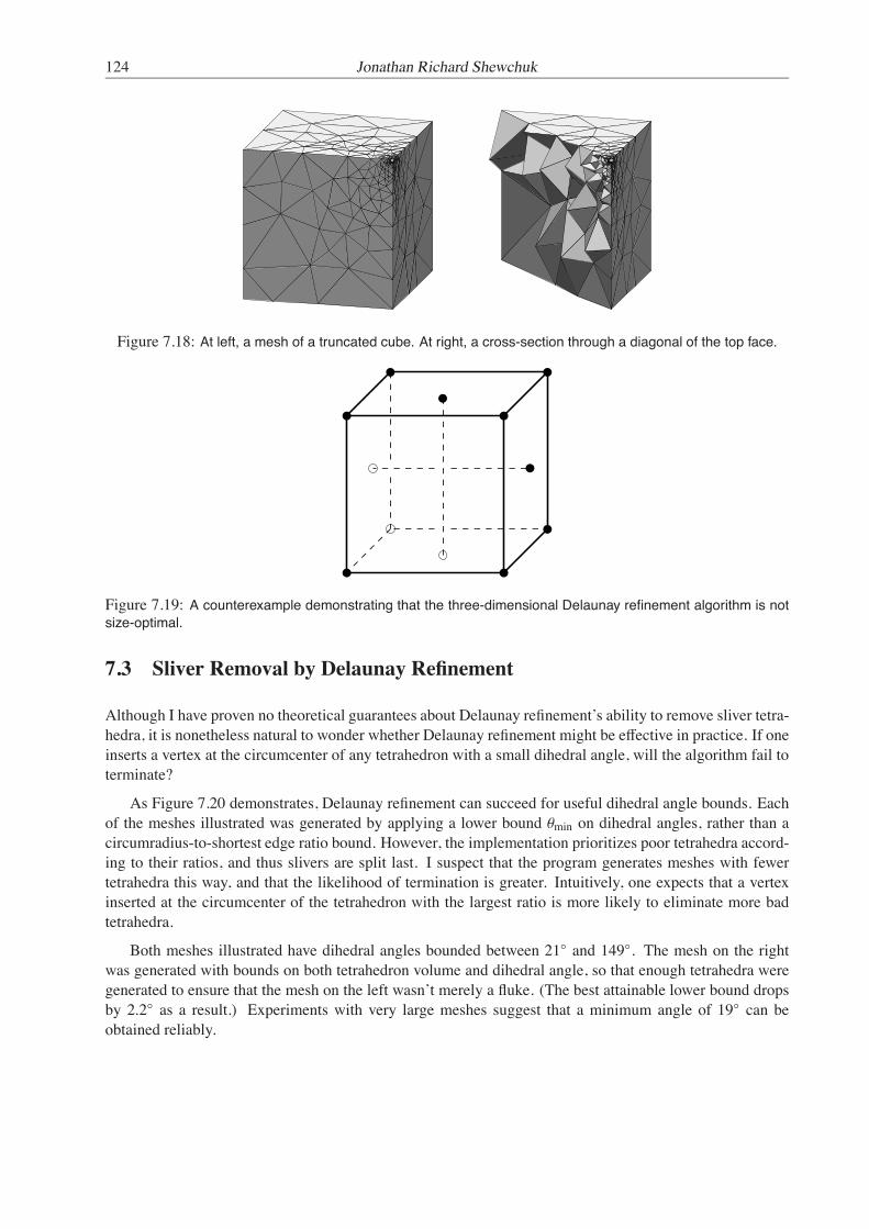
124 Jonathan Richard Shewchuk
Figure 7.18: At left, a mesh of a truncated cube. At right, a cross-section through a diagonal of the top face.
Figure 7.19: A counterexample demonstrating that the three-dimensional Delaunay refinement algorithm is notsize-optimal.
7.3 Sliver Removal by Delaunay Refinement
Although I have proven no theoretical guarantees about Delaunay refinement’s ability to remove sliver tetra-hedra, it is nonetheless natural to wonder whether Delaunay refinement might be effective in practice. If oneinserts a vertex at the circumcenter of any tetrahedron with a small dihedral angle, will the algorithm fail toterminate?
As Figure 7.20 demonstrates, Delaunay refinement can succeed for useful dihedral angle bounds. Eachof the meshes illustrated was generated by applying a lower bound θmin on dihedral angles, rather than acircumradius-to-shortest edge ratio bound. However, the implementation prioritizes poor tetrahedra accord-ing to their ratios, and thus slivers are split last. I suspect that the program generates meshes with fewertetrahedra this way, and that the likelihood of termination is greater. Intuitively, one expects that a vertexinserted at the circumcenter of the tetrahedron with the largest ratio is more likely to eliminate more badtetrahedra.
Both meshes illustrated have dihedral angles bounded between 21 and 149. The mesh on the rightwas generated with bounds on both tetrahedron volume and dihedral angle, so that enough tetrahedra weregenerated to ensure that the mesh on the left wasn’t merely a fluke. (The best attainable lower bound dropsby 2.2 as a result.) Experiments with very large meshes suggest that a minimum angle of 19 can beobtained reliably.

Sliver Removal by Delaunay Refinement 125
B = 1.88, θmin = 23.5, θmax = 144.8,hmin = 0.765, 307 vertices, 891 tetrahedra.
B = 2.02, θmin = 21.3, θmax = 148.8,hmin = 0.185, 1761 vertices, 7383 tetrahedra.
Figure 7.20: Meshes created by Delaunay refinement with bounds on the smallest dihedral angle θmin. Alsolisted for each mesh is its largest dihedral angle θmax and its shortest edge length hmin. Compare with Figure 7.17on Page 123.
Chew [38] offers hints as to why slivers might be eliminated so readily. A sliver can always be eliminatedby splitting it, but how can one avoid creating new slivers in the process? Chew observes that a newlyinserted vertex can only take part in a sliver if it is positioned badly relative to a triangular face alreadyin the mesh. Figure 7.21 illustrates the set of bad positions. At left, a side view of the plane containing aface of the tetrahedralization is drawn. A tetrahedron formed by the face and a new vertex can have a smalldihedral angle only if the new vertex lies within the slab depicted; this slab is the set of all points withina certain distance from the plane. Late in the Delaunay refinement process, such a tetrahedron can onlyarise if its circumradius-to-shortest edge ratio is small, which implies that it must lie in the region coloredblack in Figure 7.21 (left). This disallowed region, depicted at right, is shaped like a ring with an hourglasscross-section.
Chew shows that if the slab associated with each face is sufficiently thin, a randomized Delaunay re-finement algorithm can avoid ever placing a vertex in the disallowed region of any face. The key idea isthat each new vertex is not inserted precisely at a circumcenter; rather, a candidate vertex is generated at arandomly chosen location in the inner half of the circumsphere’s radius. If the candidate vertex lies in someface’s disallowed region, the candidate is rejected and a new one generated in its stead.
The algorithm will eventually generate a successful candidate, because the number of nearby triangularfaces is bounded, and the volume of each disallowed region is small. If the sum of the volumes of thedisallowed regions is less than the volume of the region in which candidate vertices are generated, a goodcandidate will eventually be found. To ensure that this condition is met, the slabs are made very thin.
Chew derives an explicit bound on the worst-case tetrahedron aspect ratio, which is too small to serveas a practical guarantee. However, there is undoubtedly a great deal of slack in the derivation. Even if theslabs are made thick enough to offer a useful bound on the minimum dihedral angle, the small volume of thedisallowed region suggests that the practical prospects are good. My non-randomized Delaunay refinementimplementation seems to verify this intuition. I have not yet tested whether randomization is helpful inpractice. Although randomization may reduce the frequency with which slivers are generated, the act ofinserting vertices off-center in circumspheres weakens the bound on circumradius-to-shortest edge ratio.
Unfortunately, my success in removing slivers is probably due in part to the severe restrictions on inputangles I have imposed. Practitioners report that they have the most difficulty removing slivers at the bound-

126 Jonathan Richard Shewchuk
Plane of
Circumcircle ofTriangular Face
Disallowed Region
Slab
TriangularFace
Figure 7.21: Left: A side view of the plane containing a triangular face. In conjunction with this face, a newlyinserted vertex can form a sliver with both a bad dihedral angle and a good circumradius-to-shortest edge ratioonly if it is inserted in the disallowed region (black). Right: An oblique view of the disallowed region of a triangularface.
ary of a mesh, especially near small angles. Mesh improvement techniques such as optimization-basedsmoothing and topological transformations can remove some of the imperfections that cannot be removeddirectly by Delaunay refinement.
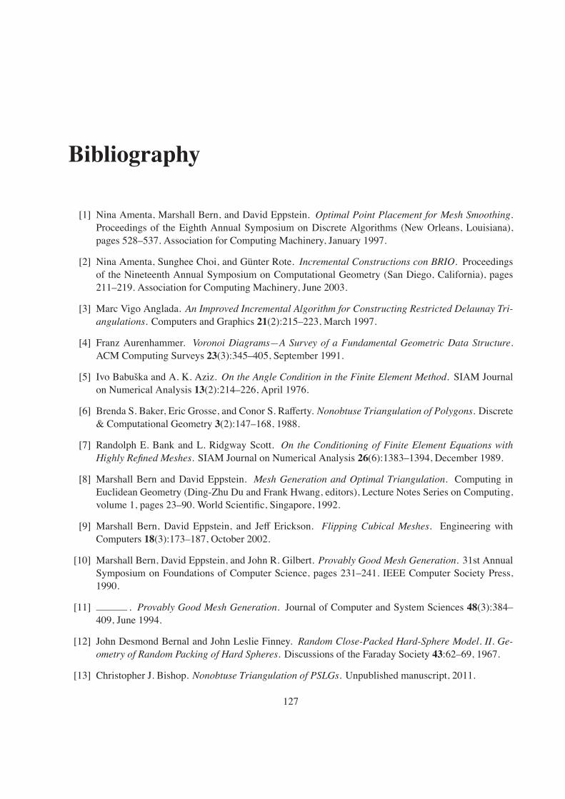
Bibliography
[1] Nina Amenta, Marshall Bern, and David Eppstein. Optimal Point Placement for Mesh Smoothing.Proceedings of the Eighth Annual Symposium on Discrete Algorithms (New Orleans, Louisiana),pages 528–537. Association for Computing Machinery, January 1997.
[2] Nina Amenta, Sunghee Choi, and Gunter Rote. Incremental Constructions con BRIO. Proceedingsof the Nineteenth Annual Symposium on Computational Geometry (San Diego, California), pages211–219. Association for Computing Machinery, June 2003.
[3] Marc Vigo Anglada. An Improved Incremental Algorithm for Constructing Restricted Delaunay Tri-angulations. Computers and Graphics 21(2):215–223, March 1997.
[4] Franz Aurenhammer. Voronoi Diagrams—A Survey of a Fundamental Geometric Data Structure.ACM Computing Surveys 23(3):345–405, September 1991.
[5] Ivo Babuska and A. K. Aziz. On the Angle Condition in the Finite Element Method. SIAM Journalon Numerical Analysis 13(2):214–226, April 1976.
[6] Brenda S. Baker, Eric Grosse, and Conor S. Rafferty. Nonobtuse Triangulation of Polygons. Discrete& Computational Geometry 3(2):147–168, 1988.
[7] Randolph E. Bank and L. Ridgway Scott. On the Conditioning of Finite Element Equations withHighly Refined Meshes. SIAM Journal on Numerical Analysis 26(6):1383–1394, December 1989.
[8] Marshall Bern and David Eppstein. Mesh Generation and Optimal Triangulation. Computing inEuclidean Geometry (Ding-Zhu Du and Frank Hwang, editors), Lecture Notes Series on Computing,volume 1, pages 23–90. World Scientific, Singapore, 1992.
[9] Marshall Bern, David Eppstein, and Jeff Erickson. Flipping Cubical Meshes. Engineering withComputers 18(3):173–187, October 2002.
[10] Marshall Bern, David Eppstein, and John R. Gilbert. Provably Good Mesh Generation. 31st AnnualSymposium on Foundations of Computer Science, pages 231–241. IEEE Computer Society Press,1990.
[11] . Provably Good Mesh Generation. Journal of Computer and System Sciences 48(3):384–409, June 1994.
[12] John Desmond Bernal and John Leslie Finney. Random Close-Packed Hard-Sphere Model. II. Ge-ometry of Random Packing of Hard Spheres. Discussions of the Faraday Society 43:62–69, 1967.
[13] Christopher J. Bishop. Nonobtuse Triangulation of PSLGs. Unpublished manuscript, 2011.
127

128 Jonathan Richard Shewchuk
[14] Ted D. Blacker and Ray J. Meyers. Seams and Wedges in Plastering: A 3-D Hexahedral MeshGeneration Algorithm. Engineering with Computers 9:83–93, 1993.
[15] Ted D. Blacker and Michael B. Stephenson. Paving: A New Approach to Automated Quadrilat-eral Mesh Generation. International Journal for Numerical Methods in Engineering 32(4):811–847,September 1991.
[16] Daniel K. Blandford, Guy E. Blelloch, David E. Cardoze, and Clemens Kadow. Compact Represen-tations of Simplicial Meshes in Two and Three Dimensions. International Journal of ComputationalGeometry and Applications 15(1):3–24, February 2005.
[17] Guy E. Blelloch, Hal Burch, Karl Crary, Robert Harper, Gary L. Miller, and Noel J. Walkington.Persistent Triangulations. Journal of Functional Programming 11(5):441–466, September 2001.
[18] Jean-Daniel Boissonnat, David Cohen-Steiner, Bernard Mourrain, Gunter Rote, and Gert Vegter.Meshing of Surfaces. Effective Computational Geometry for Curves and Surfaces (Jean-Daniel Bois-sonnat and Monique Teillaud, editors), chapter 5, pages 181–229. Springer, 2006.
[19] Charles Boivin and Carl Ollivier-Gooch. Guaranteed-Quality Triangular Mesh Generation forDomains with Curved Boundaries. International Journal for Numerical Methods in Engineering55(10):1185–1213, 20 August 2002.
[20] Adrian Bowyer. Computing Dirichlet Tessellations. Computer Journal 24(2):162–166, 1981.
[21] Kevin Q. Brown. Voronoi Diagrams from Convex Hulls. Information Processing Letters 9(5):223–228, December 1979.
[22] Scott A. Canann, S. N. Muthukrishnan, and R. K. Phillips. Topological Refinement Procedures forTriangular Finite Element Meshes. Engineering with Computers 12(3 & 4):243–255, 1996.
[23] Scott A. Canann, Michael Stephenson, and Ted Blacker. Optismoothing: An Optimization-DrivenApproach to Mesh Smoothing. Finite Elements in Analysis and Design 13:185–190, 1993.
[24] James C. Cavendish. Automatic Triangulation of Arbitrary Planar Domains for the Finite ElementMethod. International Journal for Numerical Methods in Engineering 8(4):679–696, 1974.
[25] James C. Cavendish, David A. Field, and William H. Frey. An Approach to Automatic Three-Dimensional Finite Element Mesh Generation. International Journal for Numerical Methods in En-gineering 21(2):329–347, February 1985.
[26] Donald R. Chand and Sham S. Kapur. An Algorithm for Convex Polytopes. Journal of the Associationfor Computing Machinery 17(1):78–86, January 1970.
[27] Bernard Chazelle. Convex Partitions of Polyhedra: A Lower Bound and Worst-Case Optimal Algo-rithm. SIAM Journal on Computing 13(3):488–507, August 1984.
[28] Bernard Chazelle and Leonidas Palios. Triangulating a Nonconvex Polytope. Discrete & Computa-tional Geometry 5(1):505–526, December 1990.
[29] Siu-Wing Cheng, Tamal Krishna Dey, Herbert Edelsbrunner, Michael A. Facello, and Shang-HuaTeng. Sliver Exudation. Journal of the Association for Computing Machinery 47(5):883–904,September 2000.

Bibliography 129
[30] . Sliver Exudation. Proceedings of the Fifteenth Annual Symposium on Computational Ge-ometry (Miami Beach, Florida), pages 1–13. Association for Computing Machinery, June 1999.
[31] Siu-Wing Cheng, Tamal Krishna Dey, and Edgar A. Ramos. Delaunay Refinement for PiecewiseSmooth Complexes. Discrete & Computational Geometry 43(1):121–166, 2010.
[32] Siu-Wing Cheng, Tamal Krishna Dey, Edgar A. Ramos, and Rephael Wenger. Anisotropic Sur-face Meshing. Proceedings of the Seventeenth Annual Symposium on Discrete Algorithms (Miami,Florida), pages 202–211, January 2006.
[33] Siu-Wing Cheng and Sheung-Hung Poon. Graded Conforming Delaunay Tetrahedralization withBounded Radius-Edge Ratio. Proceedings of the Fourteenth Annual Symposium on Discrete Al-gorithms (Baltimore, Maryland), pages 295–304. Society for Industrial and Applied Mathematics,January 2003.
[34] L. Paul Chew. Constrained Delaunay Triangulations. Algorithmica 4(1):97–108, 1989.
[35] . Guaranteed-Quality Triangular Meshes. Technical Report TR-89-983, Department of Com-puter Science, Cornell University, 1989.
[36] . Building Voronoi Diagrams for Convex Polygons in Linear Expected Time. Technical ReportPCS-TR90-147, Department of Mathematics and Computer Science, Dartmouth College, 1990.
[37] . Guaranteed-Quality Mesh Generation for Curved Surfaces. Proceedings of the Ninth An-nual Symposium on Computational Geometry (San Diego, California), pages 274–280. Associationfor Computing Machinery, May 1993.
[38] . Guaranteed-Quality Delaunay Meshing in 3D. Proceedings of the Thirteenth Annual Sym-posium on Computational Geometry (Nice, France), pages 391–393. Association for Computing Ma-chinery, June 1997.
[39] Kenneth L. Clarkson and Peter W. Shor. Applications of Random Sampling in Computational Geom-etry, II. Discrete & Computational Geometry 4(1):387–421, December 1989.
[40] David Cohen-Steiner, Eric Colin de Verdiere, and Mariette Yvinec. Conforming Delaunay Trian-gulations in 3D. Proceedings of the Eighteenth Annual Symposium on Computational Geometry(Barcelona, Spain), pages 199–208. Association for Computing Machinery, June 2002.
[41] Richard Courant, Kurt Friedrichs, and Hans Lewy. Uber die Partiellen Differenzengleichungen derMathematischen Physik. Mathematische Annalen 100:32–74, August 1928.
[42] Ed F. D’Azevedo and R. Bruce Simpson. On Optimal Interpolation Triangle Incidences. SIAMJournal on Scientific and Statistical Computing 10:1063–1075, 1989.
[43] Boris Nikolaevich Delaunay. Sur la Sphere Vide. Izvestia Akademia Nauk SSSR, VII Seria, OtdelenieMatematicheskii i Estestvennyka Nauk 7:793–800, 1934.
[44] Olivier Devillers. On Deletion in Delaunay Triangulations. Proceedings of the Fifteenth AnnualSymposium on Computational Geometry (Miami Beach, Florida), pages 181–188. Association forComputing Machinery, June 1999.
[45] Tamal Krishna Dey, Chanderjit L. Bajaj, and Kokichi Sugihara. On Good Triangulations in ThreeDimensions. International Journal of Computational Geometry and Applications 2(1):75–95, 1992.
130 Jonathan Richard Shewchuk
[46] Rex A. Dwyer. A Faster Divide-and-Conquer Algorithm for Constructing Delaunay Triangulations.Algorithmica 2(2):137–151, 1987.
[47] . Higher-Dimensional Voronoi Diagrams in Linear Expected Time. Discrete & Computa-tional Geometry 6(4):343–367, 1991.
[48] Herbert Edelsbrunner and Raimund Seidel. Voronoi Diagrams and Arrangements. Discrete & Com-putational Geometry 1:25–44, 1986.
[49] Herbert Edelsbrunner and Tiow Seng Tan. An Upper Bound for Conforming Delaunay Triangula-tions. Discrete & Computational Geometry 10(2):197–213, 1993.
[50] David A. Field. Qualitative Measures for Initial Meshes. International Journal for Numerical Methodsin Engineering 47:887–906, 2000.
[51] Steven Fortune. A Sweepline Algorithm for Voronoi Diagrams. Algorithmica 2(2):153–174, 1987.
[52] . Voronoi Diagrams and Delaunay Triangulations. Computing in Euclidean Geometry (Ding-Zhu Du and Frank Hwang, editors), Lecture Notes Series on Computing, volume 1, pages 193–233.World Scientific, Singapore, 1992.
[53] C. O. Frederick, Y. C. Wong, and F. W. Edge. Two-Dimensional Automatic Mesh Generation forStructural Analysis. International Journal for Numerical Methods in Engineering 2:133–144, 1970.
[54] Lori A. Freitag, Mark Jones, and Paul E. Plassmann. An Efficient Parallel Algorithm for MeshSmoothing. Fourth International Meshing Roundtable (Albuquerque, New Mexico), pages 47–58.Sandia National Laboratories, October 1995.
[55] Lori A. Freitag and Carl Ollivier-Gooch. Tetrahedral Mesh Improvement Using Swapping andSmoothing. International Journal for Numerical Methods in Engineering 40(21):3979–4002, Novem-ber 1997.
[56] William H. Frey. Selective Refinement: A New Strategy for Automatic Node Placement in GradedTriangular Meshes. International Journal for Numerical Methods in Engineering 24(11):2183–2200,November 1987.
[57] Isaac Fried. Condition of Finite Element Matrices Generated from Nonuniform Meshes. AIAAJournal 10(2):219–221, February 1972.
[58] John Alan George. Computer Implementation of the Finite Element Method. Ph.D. thesis, StanfordUniversity, Stanford, California, March 1971. Technical report STAN-CS-71-208.
[59] Nicolas Grislain and Jonathan Richard Shewchuk. The Strange Complexity of Constrained Delau-nay Triangulation. Proceedings of the Fifteenth Canadian Conference on Computational Geometry(Halifax, Nova Scotia, Canada), pages 89–93, August 2003.
[60] Leonidas J. Guibas and Jorge Stolfi. Primitives for the Manipulation of General Subdivisions and theComputation of Voronoi Diagrams. ACM Transactions on Graphics 4(2):74–123, April 1985.
[61] Carol Hazlewood. Approximating Constrained Tetrahedrizations. Computer Aided Geometric De-sign 10:67–87, 1993.

Bibliography 131
[62] Francois Hermeline. Une Methode Automatique de Maillage en Dimension n. Ph.D. thesis, UniversitePierre et Marie Curie, 1980.
[63] . Triangulation Automatique d’un Polyedre en Dimension N. RAIRO Analyse Numerique16(3):211–242, 1982.
[64] Antony Jameson, Timothy J. Baker, and Nigel P. Weatherill. Calculation of Inviscid TransonicFlow over a Complete Aircraft. Proceedings of the 24th AIAA Aerospace Sciences Meeting (Reno,Nevada), January 1986. AIAA paper 86-0103.
[65] Pierre Jamet. Estimations d’Erreur pour des Elements Finis Droits Presque Degeneres. RAIROAnalyse Numerique 10(1):43–60, 1976.
[66] Barry Joe. Three-Dimensional Triangulations from Local Transformations. SIAM Journal on Scien-tific and Statistical Computing 10:718–741, 1989.
[67] . Construction of Three-Dimensional Improved-Quality Triangulations Using Local Trans-formations. SIAM Journal on Scientific Computing 16(6):1292–1307, November 1995.
[68] H. A. Kamel and K. Eisenstein. Automatic Mesh Generation in Two- and Three-Dimensional Inter-Connected Domains. Symposium on High Speed Computing of Elastic Structures (Liege, Belgium),1970.
[69] Paul Kinney. CleanUp: Improving Quadrilateral Finite Element Meshes. Sixth International MeshingRoundtable (Park City, Utah), pages 449–461. Sandia National Laboratories, October 1997.
[70] Bryan Matthew Klingner and Jonathan Richard Shewchuk. Aggressive Tetrahedral Mesh Improve-ment. Proceedings of the 16th International Meshing Roundtable (Seattle, Washington), pages 3–23.Springer, October 2007.
[71] Michal Krızek. On the Maximum Angle Condition for Linear Tetrahedral Elements. SIAM Journalon Numerical Analysis 29(2):513–520, April 1992.
[72] Francois Labelle and Jonathan Richard Shewchuk. Anisotropic Voronoi Diagrams and Guaranteed-Quality Anisotropic Mesh Generation. Proceedings of the Nineteenth Annual Symposium on Com-putational Geometry (San Diego, California), pages 191–200. Association for Computing Machinery,June 2003.
[73] Charles L. Lawson. Software for C1 Surface Interpolation. Mathematical Software III (John R. Rice,editor), pages 161–194. Academic Press, New York, 1977.
[74] Der-Tsai Lee and Arthur K. Lin. Generalized Delaunay Triangulations for Planar Graphs. Discrete& Computational Geometry 1:201–217, 1986.
[75] Der-Tsai Lee and Bruce J. Schachter. Two Algorithms for Constructing a Delaunay Triangulation.International Journal of Computer and Information Sciences 9(3):219–242, 1980.
[76] S. H. Lo. A New Mesh Generation Scheme for Arbitrary Planar Domains. International Journal forNumerical Methods in Engineering 21(8):1403–1426, August 1985.
[77] Rainald Lohner and Paresh Parikh. Generation of Three-Dimensional Unstructured Grids by theAdvancing-Front Method. International Journal for Numerical Methods in Fluids 8:1135–1149, 1988.

132 Jonathan Richard Shewchuk
[78] David L. Marcum. Unstructured Grid Generation Using Automatic Point Insertion and Local Recon-nection. Handbook of Grid Generation (Joe F. Thompson, Bharat K. Soni, and Nigel P. Weatherill,editors), chapter 18, pages 18.1–18.31. CRC Press, 1999.
[79] D. H. McLain. Two Dimensional Interpolation from Random Data. The Computer Journal 19(2):178–181, May 1976.
[80] Elefterios A. Melissaratos. Lp Optimal d Dimensional Triangulations for Piecewise Linear Interpo-lation: A New Result on Data Dependent Triangulations. Technical Report RUU-CS-93-13, Depart-ment of Computer Science, Utrecht University, Utrecht, The Netherlands, April 1993.
[81] Gary L. Miller, Dafna Talmor, Shang-Hua Teng, and Noel J. Walkington. A Delaunay Based Nu-merical Method for Three Dimensions: Generation, Formulation, and Partition. Proceedings of theTwenty-Seventh Annual ACM Symposium on the Theory of Computing (Las Vegas, Nevada), pages683–692, May 1995.
[82] Gary L. Miller, Dafna Talmor, Shang-Hua Teng, Noel J. Walkington, and Han Wang. Control VolumeMeshes Using Sphere Packing: Generation, Refinement and Coarsening. Fifth International MeshingRoundtable (Pittsburgh, Pennsylvania), pages 47–61, October 1996.
[83] Scott A. Mitchell. Cardinality Bounds for Triangulations with Bounded Minimum Angle. Proceedingsof the Sixth Canadian Conference on Computational Geometry (Saskatoon, Saskatchewan, Canada),pages 326–331, August 1994.
[84] Scott A. Mitchell and Stephen A. Vavasis. Quality Mesh Generation in Three Dimensions. Proceed-ings of the Eighth Annual Symposium on Computational Geometry, pages 212–221, 1992.
[85] . Quality Mesh Generation in Higher Dimensions. SIAM Journal on Computing 29(4):1334–1370, 2000.
[86] D. E. Muller and Franco P. Preparata. Finding the Intersection of Two Convex Polyhedra. TheoreticalComputer Science 7:217–236, 1978.
[87] Michael Murphy, David M. Mount, and Carl W. Gable. A Point-Placement Strategy for ConformingDelaunay Tetrahedralization. Proceedings of the Eleventh Annual Symposium on Discrete Algo-rithms, pages 67–74. Association for Computing Machinery, January 2000.
[88] Friedhelm Neugebauer and Ralf Diekmann. Improved Mesh Generation: Not Simple but Good.Fifth International Meshing Roundtable (Pittsburgh, Pennsylvania), pages 257–270. Sandia NationalLaboratories, October 1996.
[89] Van Phai Nguyen. Automatic Mesh Generation with Tetrahedral Elements. International Journal forNumerical Methods in Engineering 18:273–289, 1982.
[90] V. N. Parthasarathy, C. M. Graichen, and A. F. Hathaway. A Comparison of Tetrahedron QualityMeasures. Finite Elements in Analysis and Design 15(3):255–261, January 1994.
[91] V. N. Parthasarathy and Srinivas Kodiyalam. A Constrained Optimization Approach to Finite ElementMesh Smoothing. Finite Elements in Analysis and Design 9(4):309–320, September 1991.
[92] Steven E. Pav and Noel J. Walkington. Delaunay Refinement by Corner Lopping. Proceedings of the14th International Meshing Roundtable (San Diego, California), pages 165–181. Springer, September2005.

Bibliography 133
[93] Jaime Peraire, Joaquim Peiro, L. Formaggia, Ken Morgan, and Olgierd C. Zienkiewicz. Finite El-ement Euler Computations in Three Dimensions. International Journal for Numerical Methods inEngineering 26(10):2135–2159, October 1988.
[94] Jaime Peraire, Joaquim Peiro, and Ken Morgan. Advancing Front Grid Generation. Handbook ofGrid Generation (Joe F. Thompson, Bharat K. Soni, and Nigel P. Weatherill, editors), chapter 17,pages 17.1–17.22. CRC Press, 1999.
[95] Jaime Peraire, M. Vahdati, Ken Morgan, and Olgierd C. Zienkiewicz. Adaptive Remeshing for Com-pressible Flow Computations. Journal of Computational Physics 72(2):449–466, October 1987.
[96] V. T. Rajan. Optimality of the Delaunay Triangulation in Rd. Proceedings of the Seventh AnnualSymposium on Computational Geometry (North Conway, New Hampshire), pages 357–363, June1991.
[97] Alexander Rand and Noel J. Walkington. Collars and Intestines: Practical Conformal DelaunayRefinement. Proceedings of the 18th International Meshing Roundtable (Salt Lake City, Utah), pages481–497. Springer, October 2009.
[98] Shmuel Rippa. Long and Thin Triangles Can Be Good for Linear Interpolation. SIAM Journal onNumerical Analysis 29(1):257–270, February 1992.
[99] James Martin Ruppert. Results on Triangulation and High Quality Mesh Generation. Ph.D. thesis,University of California at Berkeley, Berkeley, California, 1992.
[100] Jim Ruppert. A New and Simple Algorithm for Quality 2-Dimensional Mesh Generation. TechnicalReport UCB/CSD 92/694, University of California at Berkeley, Berkeley, California, 1992.
[101] . A New and Simple Algorithm for Quality 2-Dimensional Mesh Generation. Proceedingsof the Fourth Annual Symposium on Discrete Algorithms, pages 83–92. Association for ComputingMachinery, January 1993.
[102] . A Delaunay Refinement Algorithm for Quality 2-Dimensional Mesh Generation. Journal ofAlgorithms 18(3):548–585, May 1995.
[103] Jim Ruppert and Raimund Seidel. On the Difficulty of Triangulating Three-Dimensional NonconvexPolyhedra. Discrete & Computational Geometry 7(3):227–253, 1992.
[104] Edward A. Sadek. A Scheme for the Automatic Generation of Triangular Finite Elements. Interna-tional Journal for Numerical Methods in Engineering 15(12):1813–1822, December 1980.
[105] Robert Schneiders. Quadrilateral and Hexahedral Element Meshes. Handbook of Grid Generation(Joe F. Thompson, Bharat K. Soni, and Nigel P. Weatherill, editors), chapter 21, pages 21.1–21.27.CRC Press, 1999.
[106] E. Schonhardt. Uber die Zerlegung von Dreieckspolyedern in Tetraeder. Mathematische Annalen98:309–312, 1928.
[107] Raimund Seidel. Voronoi Diagrams in Higher Dimensions. Diplomarbeit, Institut fur Informa-tionsverarbeitung, Technische Universitat Graz, 1982.

134 Jonathan Richard Shewchuk
[108] . Constructing Higher-Dimensional Convex Hulls at Logarithmic Cost per Face. Proceedingsof the Eighteenth Annual ACM Symposium on the Theory of Computing, pages 404–413. Associa-tion for Computing Machinery, 1986.
[109] . Constrained Delaunay Triangulations and Voronoi Diagrams with Obstacles. 1978–1988Ten Years IIG (H. S. Poingratz and W. Schinnerl, editors), pages 178–191. Institute for InformationProcessing, Graz University of Technology, 1988.
[110] . Backwards Analysis of Randomized Geometric Algorithms. New Trends in Discrete andComputational Geometry (Janos Pach, editor), Algorithms and Combinatorics, volume 10, pages37–67. Springer-Verlag, Berlin, 1993.
[111] Michael Ian Shamos and Dan Hoey. Closest-Point Problems. 16th Annual Symposium on Foun-dations of Computer Science (Berkeley, California), pages 151–162. IEEE Computer Society Press,October 1975.
[112] Jonathan Richard Shewchuk. Triangle: Engineering a 2D Quality Mesh Generator and DelaunayTriangulator. Applied Computational Geometry: Towards Geometric Engineering (Ming C. Linand Dinesh Manocha, editors), Lecture Notes in Computer Science, volume 1148, pages 203–222.Springer-Verlag, Berlin, May 1996. From the First ACM Workshop on Applied Computational Ge-ometry.
[113] . Delaunay Refinement Mesh Generation. Ph.D. thesis, School of Computer Science,Carnegie Mellon University, Pittsburgh, Pennsylvania, May 1997. Available as Technical ReportCMU-CS-97-137.
[114] . Tetrahedral Mesh Generation by Delaunay Refinement. Proceedings of the Fourteenth An-nual Symposium on Computational Geometry (Minneapolis, Minnesota), pages 86–95. Associationfor Computing Machinery, June 1998.
[115] . Sweep Algorithms for Constructing Higher-Dimensional Constrained Delaunay Triangula-tions. Proceedings of the Sixteenth Annual Symposium on Computational Geometry (Hong Kong),pages 350–359. Association for Computing Machinery, June 2000.
[116] . What Is a Good Linear Element? Interpolation, Conditioning, and Quality Measures.Eleventh International Meshing Roundtable (Ithaca, New York), pages 115–126. Sandia NationalLaboratories, September 2002.
[117] . Updating and Constructing Constrained Delaunay and Constrained Regular Triangulationsby Flips. Proceedings of the Nineteenth Annual Symposium on Computational Geometry (San Diego,California), pages 181–190. Association for Computing Machinery, June 2003.
[118] . General-Dimensional Constrained Delaunay Triangulations and Constrained Regular Tri-angulations I: Combinatorial Properties. Discrete & Computational Geometry 39(1–3):580–637,March 2008.
[119] Matthew L. Staten, Steven J. Owen, and Ted D. Blacker. Paving & Plastering: Progress Update.Proceedings of the 15th International Meshing Roundtable (Birmingham, Alabama), pages 469–486.Springer, September 2006.
Bibliography 135
[120] Peter Su and Robert L. Scot Drysdale. A Comparison of Sequential Delaunay Triangulation Algo-rithms. Proceedings of the Eleventh Annual Symposium on Computational Geometry (Vancouver,British Columbia, Canada), pages 61–70. Association for Computing Machinery, June 1995.
[121] Garret Swart. Finding the Convex Hull Facet by Facet. Journal of Algorithms 6(1):17–48, March1985.
[122] J. L. Synge. The Hypercircle in Mathematical Physics. Cambridge University Press, New York, 1957.
[123] Masaharu Tanemura, Tohru Ogawa, and Naofumi Ogita. A New Algorithm for Three-DimensionalVoronoi Tessellation. Journal of Computational Physics 51(2):191–207, August 1983.
[124] Joe F. Thompson. The National Grid Project. Computer Systems in Engineering 3(1–4):393–399,1992.
[125] Joe F. Thompson, Bharat K. Soni, and Nigel P. Weatherill, editors. Handbook of Grid Generation.CRC Press, 1999.
[126] Joe F. Thompson and Nigel P. Weatherill. Aspects of Numerical Grid Generation: Current Scienceand Art. Eleventh AIAA Applied Aerodynamics Conference, pages 1029–1070, 1993. AIAA paper93-3593-CP.
[127] Shayne Waldron. The Error in Linear Interpolation at the Vertices of a Simplex. SIAM Journal onNumerical Analysis 35(3):1191–1200, 1998.
[128] David F. Watson. Computing the n-dimensional Delaunay Tessellation with Application to VoronoiPolytopes. Computer Journal 24(2):167–172, 1981.
[129] Nigel P. Weatherill, O. Hassan, David L. Marcum, and M. J. Marchant. Grid Generation by theDelaunay Triangulation. Von Karman Institute for Fluid Dynamics 1993–1994 Lecture Series, 1994.
[130] Mark A. Yerry and Mark S. Shephard. A Modified Quadtree Approach to Finite Element MeshGeneration. IEEE Computer Graphics and Applications 3:39–46, January/February 1983.
[131] . Automatic Three-Dimensional Mesh Generation by the Modified-Octree Technique. Inter-national Journal for Numerical Methods in Engineering 20(11):1965–1990, November 1984.