Lecture Notes - Information Management Systems & Services
178
Ma/CS 6c Notes Alexander S. Kechris with Michael A. Shulman and Andr´ es E. Caicedo April 2, 2008
Transcript of Lecture Notes - Information Management Systems & Services

Ma/CS 6c Notes
Alexander S. Kechriswith Michael A. Shulmanand Andres E. Caicedo
April 2, 2008


Contents
1 Propositional Logic 11.1 Introduction . . . . . . . . . . . . . . . . . . . . . . . . . . . . 11.2 Syntax of propositional logic . . . . . . . . . . . . . . . . . . . 4
1.2.A The Language of Propositional Logic . . . . . . . . . . 41.2.B Induction on Formulas . . . . . . . . . . . . . . . . . . 61.2.C Unique Readability . . . . . . . . . . . . . . . . . . . . 71.2.D Recursive Definitions . . . . . . . . . . . . . . . . . . . 81.2.E Recognizing Formulas . . . . . . . . . . . . . . . . . . 11
1.3 Polish and Reverse Polish notation . . . . . . . . . . . . . . . 131.3.A Polish Notation . . . . . . . . . . . . . . . . . . . . . . 131.3.B Reverse Polish notation . . . . . . . . . . . . . . . . . . 16
1.4 Abbreviations . . . . . . . . . . . . . . . . . . . . . . . . . . . 211.5 Semantics of Propositional Logic . . . . . . . . . . . . . . . . 21
1.5.A Valuations . . . . . . . . . . . . . . . . . . . . . . . . . 211.5.B Models and Tautologies . . . . . . . . . . . . . . . . . 251.5.C Logical Implication and Equivalence . . . . . . . . . . 28
1.6 Truth Functions . . . . . . . . . . . . . . . . . . . . . . . . . . 311.6.A Truth Functions . . . . . . . . . . . . . . . . . . . . . . 311.6.B Completeness of Binary Connectives . . . . . . . . . . 371.6.C Normal Forms . . . . . . . . . . . . . . . . . . . . . . . 38
1.7 Konig’s Lemma and Applications . . . . . . . . . . . . . . . . 411.7.A Graphs and Trees . . . . . . . . . . . . . . . . . . . . . 411.7.B Konig’s Lemma . . . . . . . . . . . . . . . . . . . . . . 431.7.C Domino Tilings . . . . . . . . . . . . . . . . . . . . . . 451.7.D Compactness of [0, 1] . . . . . . . . . . . . . . . . . . . 49
1.8 The Compactness Theorem . . . . . . . . . . . . . . . . . . . 501.8.A The Compactness Theorem . . . . . . . . . . . . . . . 50
i

ii CONTENTS
1.8.B A Proof of Konig’s Lemma . . . . . . . . . . . . . . . . 511.8.C Partial Orders . . . . . . . . . . . . . . . . . . . . . . . 52
1.9 Ramsey Theory . . . . . . . . . . . . . . . . . . . . . . . . . . 551.9.A Ramsey Theorem, infinite version . . . . . . . . . . . . 551.9.B Ramsey Theorem, finite version . . . . . . . . . . . . . 561.9.C A few other applications of compactness . . . . . . . . 57
1.10 The Resolution Method . . . . . . . . . . . . . . . . . . . . . 581.11 A Hilbert-Type Proof System . . . . . . . . . . . . . . . . . . 66
1.11.A Formal Proofs . . . . . . . . . . . . . . . . . . . . . . . 671.11.B Soundness . . . . . . . . . . . . . . . . . . . . . . . . . 691.11.C Completeness . . . . . . . . . . . . . . . . . . . . . . . 701.11.D General Completeness . . . . . . . . . . . . . . . . . . 73
2 First-Order Logic 752.1 Structures . . . . . . . . . . . . . . . . . . . . . . . . . . . . . 75
2.1.A Relations and Functions . . . . . . . . . . . . . . . . . 752.1.B Structures . . . . . . . . . . . . . . . . . . . . . . . . . 772.1.C Introduction to First-Order Languages . . . . . . . . . 80
2.2 Syntax of First-Order Logic . . . . . . . . . . . . . . . . . . . 812.2.A Symbols . . . . . . . . . . . . . . . . . . . . . . . . . . 812.2.B Terms . . . . . . . . . . . . . . . . . . . . . . . . . . . 822.2.C Well-Formed Formulas . . . . . . . . . . . . . . . . . . 842.2.D Scope and Free Variables . . . . . . . . . . . . . . . . . 87
2.3 Semantics of First-Order Logic . . . . . . . . . . . . . . . . . . 882.3.A Structures and Interpretations . . . . . . . . . . . . . . 882.3.B Models and Validities . . . . . . . . . . . . . . . . . . . 90
2.4 Definability in a Structure . . . . . . . . . . . . . . . . . . . . 962.4.A First-Order Definability . . . . . . . . . . . . . . . . . 962.4.B Isomorphisms . . . . . . . . . . . . . . . . . . . . . . . 100
2.5 Prenex Normal Forms and Games . . . . . . . . . . . . . . . . 1032.5.A Prenex Normal Forms . . . . . . . . . . . . . . . . . . 1032.5.B Games and Strategies . . . . . . . . . . . . . . . . . . . 107
2.6 Theories . . . . . . . . . . . . . . . . . . . . . . . . . . . . . . 1102.7 A Proof System for First-Order Logic . . . . . . . . . . . . . . 115
2.7.A Formal Proofs . . . . . . . . . . . . . . . . . . . . . . . 1152.7.B Examples of Formal Proofs . . . . . . . . . . . . . . . . 1182.7.C Metatheorems . . . . . . . . . . . . . . . . . . . . . . . 119
2.8 The Godel Completeness Theorem . . . . . . . . . . . . . . . 123

CONTENTS iii
2.9 The Compactness Theorem . . . . . . . . . . . . . . . . . . . 1312.9.A Finiteness and Infinity . . . . . . . . . . . . . . . . . . 1322.9.B Non-standard Models of Arithmetic . . . . . . . . . . . 133
3 Computability and Complexity 1393.1 Introduction . . . . . . . . . . . . . . . . . . . . . . . . . . . . 1393.2 Decision Problems . . . . . . . . . . . . . . . . . . . . . . . . 1403.3 Turing Machines . . . . . . . . . . . . . . . . . . . . . . . . . 1423.4 The Church-Turing Thesis . . . . . . . . . . . . . . . . . . . . 145
3.4.A Register Machines . . . . . . . . . . . . . . . . . . . . . 1453.4.B The Church-Turing Thesis . . . . . . . . . . . . . . . . 148
3.5 Universal Machines . . . . . . . . . . . . . . . . . . . . . . . . 1493.6 The Halting Problem . . . . . . . . . . . . . . . . . . . . . . . 1503.7 Undecidability of the Validity Problem . . . . . . . . . . . . . 1513.8 The Hilbert Tenth Problem . . . . . . . . . . . . . . . . . . . 1563.9 Decidable Problems . . . . . . . . . . . . . . . . . . . . . . . . 1563.10 The Class P . . . . . . . . . . . . . . . . . . . . . . . . . . . . 1583.11 The Class NP and the P = NP Problem . . . . . . . . . . . 1603.12 NP-Complete Problems . . . . . . . . . . . . . . . . . . . . . 161
A Tautologies and equivalences 167A.1 Tautologies . . . . . . . . . . . . . . . . . . . . . . . . . . . . 167A.2 Equivalences . . . . . . . . . . . . . . . . . . . . . . . . . . . . 169
B Validities in First Order Logic 171

iv CONTENTS

Chapter 1
Propositional Logic
1.1 Introduction
A proposition is a statement which is either true or false.
Examples 1.1.1“There are infinitely many primes”; “5 > 3”; and “14 is a square number”are propositions. A statement like “x is odd,” however, is not a proposition(but it becomes one when x is substituted by a particular number).
A propositional connective is a way of combining propositions so that thetruth or falsity of the compound proposition depends only on the truth orfalsity of the components. The most common connectives are:
connective symbolnot (negation) ¬and (conjunction) ∧or (disjunction) ∨implies (implication) ⇒iff (equivalence) ⇔
Notice that each connective has a symbol which is traditionally usedto represent it. This way we can distinguish between the desired precisemathematical meaning of the connective (e.g. ¬) and the possibly vagueor ambiguous meaning of an english word (e.g. “implies”). The intendedmathematical meanings of the connectives are as follows:
1

2 CHAPTER 1. PROPOSITIONAL LOGIC
• “Not” (¬) is the only common unary connective: it applies to onlyone proposition, and negates its truth value. The others are binaryconnectives that apply to two propositions:
• A proposition combined with “and” (∧) is true only if both of its com-ponents are true, while. . .
• A proposition combined with “or” (∨) is true whenever either or bothof its components are true. That is, ∨ is the so-called “inclusive or”.
• The “iff” (short for for “if and only if”) or equivalence connective (⇔)is true whenever both of its components have the same truth value:either both true or both false.
• The “implication” connective is the only common binary connectivewhich is not symmetric: p ⇒ q is not the same as q ⇒ p. p ⇒ q isintended to convey the meaning that whenever p is true, q must alsobe. So if p is true, p ⇒ q is true if and only if q is also true. If, onthe other hand, p is false, we say that p ⇒ q is “vacuously” true. Thestatement that p ⇒ q does not carry any “causal” connotation, unlikethe English phrases we use (for lack of anything better) to pronounceit (such as “p implies q” or “if p, then q”).
We can summarize the meanings of these connectives using truth tables :
p ¬pT FF T
p q p ∧ q p ∨ q p ⇒ q p ⇔ qT T T T T TT F F T F FF T F T T FF F F F T T
Examples 1.1.2“¬2 = 2” is false;“25 = 52 ∧ 6 > 5” is true;“5 is even ∨ 16 is a square” is true;“5 is odd ∨ 16 is a square” is true;

1.1. INTRODUCTION 3
“(the square of an odd number is odd)⇒(25 is odd)” is true;“(the square of an odd number is even)⇒(25 is odd)” is true;“(the square of an odd number is odd)⇒(10 is odd)”is false.
There are many different ways to express a compound statement, andcorresponding to these there are different ways to combine propositions usingthese connectives which are equivalent : their truth values are the same forany truth values of the original propositions. Here are some examples:
(i) The statements “The cafeteria either has no pasta, or it has no sauce”and “The cafeteria doesn’t have both pasta and sauce” are two waysto say the same thing. If p = “The cafeteria has pasta” and q = “Thecafeteria has sauce”, then this means that
(¬p) ∨ (¬q) and ¬(p ∧ q)
are equivalent. This is one of what are known as De Morgan’s Laws.
(ii) The law of the double negative says that ¬¬p and p are equivalent.That is, if something is not false, it is true, and vice versa.
(iii) The statements “If it rained this morning, the grass is wet” and “If thegrass is dry, it didn’t rain this morning” are two more ways to say thesame thing. Now if p = “It rained this morning” and q = “The grassis wet”, then this means that
(p ⇒ q) and (¬q) ⇒ (¬p)
are equivalent. The latter statement is called the contrapositive of thefirst. Note that because of the law of the double negative, the firststatement is also equivalent to the contrapositive of the second.
(iv) Yet another way to say the same thing is “Either it did not rain thismorning, or the grass is wet.” That is, another proposition equivalentto those above is
(¬p) ∨ q.
One consequence of this is that we could, if we wanted to, do with-out the ⇒ connective altogether. We will see more about this in sec-tion 1.6.B.

4 CHAPTER 1. PROPOSITIONAL LOGIC
(v) Two more related statements which are not equivalent to p ⇒ q are theconverse, q ⇒ p (“If the grass is wet, it rained this morning”), and theinverse, (¬p) ⇒ (¬q) (“If it didn’t rain this morning, the grass isn’twet”). There might, for example, be sprinklers that keep the grass weteven when it doesn’t rain. The converse and inverse are contrapositivesof each other, however, so they have the same truth value.
In section 1.5 we will revisit this notion of “equivalence” in a formalcontext.
1.2 Syntax of propositional logic
In order to rigorously prove results about the structure and truth of propo-sitions and their connectives, we must set up a mathematical structure forthem. We do this with a formal language, the language of propositional logic,which we will work with for the rest of the chapter.
1.2.A The Language of Propositional Logic
Definition 1.2.1 A formal language consists of a set of symbols togetherwith a set of rules for forming “grammatically correct” strings of symbols inthis language.
Definition 1.2.2 In the language of propositional logic we have the followinglist of symbols:
(i) propositional variables : this is an infinite list p1, p2, p2, . . . of symbols.We often use p, q, r, . . . to denote propositional variables.
(ii) symbols for the (common) propositional connectives : ¬,∧,∨,⇒,⇔.
(iii) parentheses : (, ).
Definition 1.2.3 A string or word in a formal language is any finite se-quence of the symbols in the language. We include in this the empty stringcontaining no symbols at all.
Example 1.2.4 The following are examples of strings in the language ofpropositional logic:

1.2. SYNTAX OF PROPOSITIONAL LOGIC 5
p∨, pq ⇒, pqr, (p ∧ q), p)
Definition 1.2.5 If S = s1 . . . sn is a string with n symbols, we call n thelength of S and denote it by |S|. The length of the empty string is 0.
We will next specify the rules for forming “grammatically correct” stringsin propositional logic, which we call well-formed formulas (wff s) or just for-mulas.
Definition 1.2.6 (Well-Formed Formulas)(i) Every propositional variable p is a wff.
(ii) If A is a wff, so is ¬A.
(iii) If A,B are formulas, so are (A∧B), (A∨B), (A ⇒ B), and (A ⇔ B).
Thus a string A is a wff exactly when there is a finite sequence
A1, . . . , An
(called a parsing sequence) such that An = A and for each 1 ≤ i ≤ n, Ai iseither (1) a propositional variable, (2) for some j < i, Ai = ¬Aj, or (3) forsome j, k < i, Ai = (Aj ∗ Ak), where ∗ is one of ∧,∨,⇒,⇔.
Examples 1.2.7(i) (p ⇒ (q ⇒ r)) is a wff with parsing sequence
p, q, r, (q ⇒ r), (p ⇒ (q ⇒ r)).
(Also note that
q, r, (q ⇒ r), p, (p ⇒ (q ⇒ r))
is another parsing sequence, so parsing sequences are not unique.)
(ii) (¬(p ∧ q) ⇔ (¬p ∨ ¬q)) is a wff with parsing sequence
p, q, (p ∧ q), ¬(p ∧ q), ¬p, ¬q, (¬p ∨ ¬q), (¬(p ∧ q) ⇔ (¬p ∨ ¬q)).
(iii) p ⇒ qr, )p ⇔, ∨(q¬), and p ∧ q ∨ r are not wff, but to prove this israther more tricky. We will see some ways to do this in section 1.2.B.

6 CHAPTER 1. PROPOSITIONAL LOGIC
Remark. We have not yet assigned any “meaning” to any of the symbolsin our formal language. While we intend to interpret symbols such as ∨and ⇒ eventually in a way analogous to the propositional connectives “or”and “implies” in section 1.1, at present they are simply symbols that we aremanipulating formally.
1.2.B Induction on Formulas
We can prove properties of formulas by induction on the length of a formula.Suppose Φ(A) is a property of a formula A. For example, Φ(A) could mean“A has the same number of left and right parentheses.” If Φ(A) holds forall formulas of length 1 (i.e. the propositional variables) and whenever Φ(A)holds for all formulas A of length ≤ n, then it holds for all formulas of lengthn + 1, we may conclude, by the principle of mathematical induction, thatΦ(A) holds for all formulas.
However, because of the way formulas are defined, it is most useful to useanother form of induction, sometimes called induction on the construction ofwff (or just induction on formulas):
Let Φ(A) be a property of formulas A. Suppose:
(i) Basis of the induction: Φ(A) holds, when A is a propositional variable.
(ii) Induction step: If Φ(A), Φ(B) hold for two formulas A, B, then
Φ(¬A), Φ((A ∗B))
hold as well, where ∗ is one of the binary connectives ∧,∨,⇒,⇔.
Then Φ(A) holds for all formulas A. We can prove the validity of thisprocedure using standard mathematical induction, and the existence of aparsing sequence for any wff.
Example 1.2.8 One can easily prove, using this form of induction, thatevery formula A has the same number of left and right parentheses. Thisresult can be used to show that certain strings, for example )p ⇔, are notwffs, because they have unequal numbers of left and right parentheses.
Example 1.2.9 If s1s2 . . . sn is any string, then an initial segment of it isa string s1 . . . sm, where 0 ≤ m ≤ n (when m = 0, this means the emptystring). If m < n we call this a proper initial segment.

1.2. SYNTAX OF PROPOSITIONAL LOGIC 7
Again we can easily prove by induction on the construction of wff that anonempty proper initial segment of a formula either consists of a string of ¬’sor else has more left than right parentheses. (To see some examples, consider¬¬(p ⇒ q), ((p ⇒ (q ∧ p)) ⇒ ¬p).) Another easy induction shows thatno formula can be empty or just a string of ¬’s, so using also the previousexample, no proper initial segment of a wff is a wff.
This can also be used to show certain strings (for example, p ⇒ qr) arenot wffs, as they contain proper initial segments that are wffs (in the example,p). Similar methods can be used for other non-wffs.
1.2.C Unique Readability
While parsing sequences are not unique, as mentioned in examples 1.2.7,there is a sense in which both alternative parsing sequences offered are “thesame”: they break the wff down in the same way, to the same components,albeit in a different order. Using induction on formulas, we can prove thatthis will always be the case. This is called unique readability.
Theorem 1.2.10 (Unique Readability Theorem) Every wff is in exact-ly one of the forms:
(i) p (i.e., a propositional variable);
(ii) ¬A for A a uniquely determined wff;
(iii) (A ∗ B), for uniquely determined wff’s A,B and uniquely determined∗ ∈ {∧,∨,⇒,⇔}.
Proof. By induction on the construction of formulas, it is straightforwardthat any formula must be of one of these forms. To prove uniqueness firstnotice that no wff can be in more than one of the forms (i), (ii), (iii). Andobviously no two propositional variables are the same, and if ¬A = ¬B, thenA = B.
So it is enough to show that in case (iii), if (A ∗ B) = (C ◦ D), for∗, ◦ ∈ {∧,∨,⇒,⇔}, then A = C,B = D and ∗ = ◦. First notice that, byeliminating the left parenthesis, we have that A ∗B) = C ◦D). From this itfollows that either A is an initial segment of C or vice versa. If A 6= C, thenone of A,C is a proper initial segment of the other, which is impossible, asthey are both formulas. So we must have A = C. Thus ∗B) = ◦D) and so∗ = ◦ and B = D. a

8 CHAPTER 1. PROPOSITIONAL LOGIC
Definition 1.2.11 In form (ii) we call ¬ the main connective and in (iii)we call ∗ the main connective. (Thus the main connective is the one appliedlast.)
Example 1.2.12 In ((p ⇒ (q ⇒ p)) ⇒ q) the main connective is the third“⇒” (from left to right).
Given a formula A, it might be hard to recognize immediately which isthe main connective. Consider for example the following formula:
(((((p ∨ ¬q) ∨ ¬r) ∧ ((¬p ∨ (s ∨ ¬r)) ∧ ((q ∨ s) ∨ p)))∧(((¬q ∨ ¬r) ∨ s) ∧ (s ∨ (¬r ∨ q)))) ∧ ((p ∨ (¬r ∨ s)) ∧ (s ∨ ¬r)))
(it turns out to be the 5th “∧”). There is however an easy algorithm fordetermining the main connective: In the formula (A∗B) the main connective∗ is the first binary connective (from left-to-right) such that in the stringpreceding it the number of left parentheses is exactly one more than thenumber of right parentheses.
1.2.D Recursive Definitions
Often we will want to define a function or characteristic of wffs, and the mostnatural way to do it is to break down the formula into simpler formulas onestep at a time. To make this rigorous, we can use the unique readabilitytheorem to justify the following principle of definition by recursion on theconstruction of formulas :
Let X be a set and
f : {p1, p2, . . . } → X
f¬ : X → X
f∧, f∨, f⇒, f⇔ : X2 → X
be given functions. Then there is a unique function g from the set of allformulas into X such that
g(p) = f(p)
g(¬A) = f¬(g(A))
g((A ∗B)) = f∗(g(A), g(B)), ∗ ∈ {∧,∨,⇒,⇔}.
1.2. SYNTAX OF PROPOSITIONAL LOGIC 9
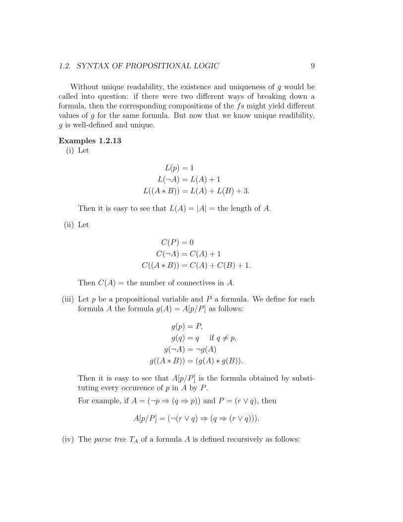
Without unique readability, the existence and uniqueness of g would becalled into question: if there were two different ways of breaking down aformula, then the corresponding compositions of the fs might yield differentvalues of g for the same formula. But now that we know unique readibility,g is well-defined and unique.
Examples 1.2.13(i) Let
L(p) = 1
L(¬A) = L(A) + 1
L((A ∗B)) = L(A) + L(B) + 3.
Then it is easy to see that L(A) = |A| = the length of A.
(ii) Let
C(P ) = 0
C(¬A) = C(A) + 1
C((A ∗B)) = C(A) + C(B) + 1.
Then C(A) = the number of connectives in A.
(iii) Let p be a propositional variable and P a formula. We define for eachformula A the formula g(A) = A[p/P ] as follows:
g(p) = P,
g(q) = q if q 6= p,
g(¬A) = ¬g(A)
g((A ∗B)) = (g(A) ∗ g(B)).
Then it is easy to see that A[p/P ] is the formula obtained by substi-tuting every occurence of p in A by P .
For example, if A = (¬p ⇒ (q ⇒ p)) and P = (r ∨ q), then
A[p/P ] = (¬(r ∨ q) ⇒ (q ⇒ (r ∨ q))).
(iv) The parse tree TA of a formula A is defined recursively as follows:

10 CHAPTER 1. PROPOSITIONAL LOGIC
Tp : p
T¬A :
TA
¬¬A
T(A∗B) :
TA TB
(A ∗B)
∗
For example, if A = (¬(p ∧ q) ⇔ (¬p ∨ ¬q)), then its parse tree is
p q
(p ∧ q)
∧
¬¬(p ∧ q)
p
¬¬p
q
¬¬q
(¬p ∨ ¬q)
∨
A⇔
The parse tree, starting now from the bottom up, gives us various waysof constructing a parsing sequence for the formula; for example:
p, q, (p ∧ q), ¬(p ∧ q), ¬p, ¬q, (¬p ∨ ¬q), (¬(p ∧ q) ⇔ (¬p ∨ ¬q)).
By unique readability, all parsing sequences can be obtained in thismanner. Thus the parse tree extracts the “common part” out of eachparsing sequence.

1.2. SYNTAX OF PROPOSITIONAL LOGIC 11
(v) The formulas occurring in the parse tree of a formula A are called thesubformulas of A. These are the formulas that arise in the constructionof A. If we let subf(A) denote the set of subformulas of A, then subfcan be defined by the following recursion:
subf(p) = {p}subf(¬A) = subf(A) ∪ {¬A}
subf((A ∗B)
)= subf(A) ∪ subf(B) ∪ {(A ∗B)}.
1.2.E Recognizing Formulas
We will next discuss an algorithm for verifying that a given string is a formula.
Algorithm 1.2.14 Given a string S, let x be a propositional variable notoccurring in S and let S(x) the string we obtain from S by substituting everypropositional variable by x.
For any string T containing only the variable x, let T ′ be the stringobtained from T as follows: If T contains no substring (i.e. a string containedin T as a consecutive sequence of symbols) of the form ¬x, (x∧x), (x∨x), (x ⇒x), (x ⇔ x), then T ′ = T . Otherwise substitute the leftmost occurence of anyone of these forms by x, to obtain T ′. Notice that if T 6= T ′, then |T ′| < |T |.
Now starting with an arbitrary string S, form first S(x), and then definerecursively S0 = S(x), Sn+1 = S ′n. This process stops when we hit n0 forwhich Sn0+1 = S ′n0
= Sn0 , i.e., Sn has no substring of the above form. Thismust necessarily happen since otherwise we would have |S0| > |S1| > . . . (adinfinitum), which is impossible.
We now claim that if Sn0 = x, then S is a formula, otherwise it is not.
Examples 1.2.15(i) ((p ⇒ (q ∨ ¬p) ⇒ (r ∨ (¬s ⇒ t)))) = S
((x ⇒ (x ∨ ¬x) ⇒ (x ∨ (¬x ⇒ x)))) = S(x) = S0
((x ⇒ (x ∨ x) ⇒ (x ∨ (¬x ⇒ x)))) = S1
((x ⇒ x ⇒ (x ∨ (¬x ⇒ x)))) = S2
((x ⇒ x ⇒ (x ∨ (x ⇒ x)))) = S3
((x ⇒ x ⇒ (x ∨ x))) = S4
((x ⇒ x ⇒ x)) = S5 = S6

12 CHAPTER 1. PROPOSITIONAL LOGIC
So S is not a wff.
(ii) ((p ⇒ ¬q) ⇒ (p ∨ (¬r ∧ s))) = S
((x ⇒ ¬x) ⇒ (x ∨ (¬x ∧ x))) = S(x) = S0
((x ⇒ x) ⇒ (x ∨ (¬x ∧ x))) = S1
(x ⇒ (x ∨ (¬x ∧ x))) = S2
((x ⇒ (x ∨ (x ∧ x))) = S3
((x ⇒ (x ∨ x)) = S4
(x ⇒ x) = S5
x = S6 = S7
So S is a wff.
We will now prove the correctness of this algorithm in two parts: first,that it recognizes all wffs, and second, that it recognizes only wffs.
Part I. If S = A is a wff, then this process stops at x.
Proof of part I. First notice that S is a wff iff S(x) is a wff. (This can beeasily proved by induction on the construction of formulas.)
So if A is a wff, so is B = A(x). Thus it is enough to show that ifwe start with any wff B containing only the variable x and we performthis process, we will end up with x. For this it is enough to show that forany such formula B, B′ is also a formula. Because then when the processB0 = B, B1, . . . , Bn0 stops, we have that Bn0 is a formula containing onlythe variable x and B′
n0= Bn0 , i.e., Bn0 contains no substrings of the form
¬x, (x ∧ x), (x ∨ x), (x ⇒ x), (x ⇔ x), therefore it must be equal to x.We can prove that for any formula B, B′ is a formula, by induction on
the construction of B. If B = x, then B′ = B = x. If B = ¬C, then eitherC = x and B′ = x, or else B′ = ¬C ′, since C 6= x implies that C cannotstart with x. If B = (C ∗D), then, unless C = D = x, in which case B′ = x,either B′ = (C ′ ∗D) or B′ = (C ∗D′). aPart II. If, starting from S, this process terminates at x, then S is aformula.
Proof of part II. Again we can assume that we start with a string S0
containing only the variable x and show that if S0, S1, . . . , Sn0 = S ′n0= x, for
some n0, where Sn+1 = S ′n, then S0 is a formula. To see this notice that Sn0 isa formula and Sn−1 is obtained from Sn by substituting some occurrence x by

1.3. POLISH AND REVERSE POLISH NOTATION 13
a formula. So working backwards, and using the fact that if in a wff we sub-stitute an occurrence of a variable by a formula we still get a formula (a factwhich is easy to prove by induction), we see that Sn0 , Sn0−1, Sn0−2, . . . , S1, S0
are all formulas. a
1.3 Polish and Reverse Polish notation
We will now describe two different ways of writing formulas in which paren-theses can be avoided. These methods are often better suited to computerprocessing, and many computer programs store formulas internally in one ofthese notations, even if they use standard notation for input and output.
1.3.A Polish Notation
We define a new formal language as follows:
(i) The symbols are the same as before, except that there are no paren-theses, i.e.:
p1, p2, . . . ,¬,∧,∨,⇒,⇔
(ii) We have the following rules for forming grammatically correct formulas,which we now call Polish wff or just P-wff or P-formulas :
(a) Every propositional variable p is a P-wff;
(b) If A is a P-wff, so is ¬A.
(c) If A,B are P-wff, so is ∗AB, where ∗ ∈ {∧,∨,⇒,⇔}
Remark. Polish notation is named after the Polish logician ÃLukasiewiczwho first introduced it, although he used N , K, A, C, and E in place of ¬,∧, ∨, ⇒, and ⇔ respectively.
Example 1.3.1
⇒⇒ s¬t¬ ∨ p ∧ ¬qs
is a P-wff as the following parsing sequence demonstrates
q, ¬q, s, ∧¬qs, p, ∨p ∧ ¬qs, ¬ ∨ p ∧¬qs, t, ¬t, ⇒ s¬t, ⇒⇒ s¬t¬ ∨ p ∧¬qs.

14 CHAPTER 1. PROPOSITIONAL LOGIC
In ordinary notation this P-wff corresponds to the wff:
((s ⇒ ¬t) ⇒ ¬(p ∨ (¬q ∧ s))).
As with regular formulas, we have unique readability.
Theorem 1.3.2 (Unique Readability of P-wff) Every P-wff A is in ex-actly one of the forms,
(i) p
(ii) ¬B
(iii) ∗BC, where ∗ ∈ {∧,∨,⇒,⇔}, for uniquely determined P-wff B, C.
Proof. Clearly the only thing we have to prove is that if B, C, B′, C ′ areP-wff and BC = B′C ′, then B = B′, C = C ′. If BC = B′C ′ then one ofB, B′ is an initial segment of the other, so it is enough to prove the followinglemma:
Lemma 1.3.3 No nonempty proper initial segment of a P-wff is a P-wff.
Proof of Lemma 1.3.3. We define a weight for each symbol as follows:
w(p) = 1
w(¬) = 0
w(∗) = −1 if ∗ ∈ {∧,∨,⇒,⇔}.
Then we define the weight of any string S = s1s2 . . . sn, by
w(S) =n∑
i=1
w(si).
For example, w(∧ ⇒ s¬pq) = 1. It is easy to show by induction on theconstruction of a P-wff that if A is a P-wff, then w(A) = 1.
We now define a terminal segment of a string S = s1 . . . sn to be anystring of the form
smsm+1 . . . sn (1 ≤ m ≤ n)

1.3. POLISH AND REVERSE POLISH NOTATION 15
or the empty string. The concatenation of strings S1, . . . , Sk is the stringS1S2 . . . Sk, which consists of the symbols of S1 followed by those of S2, andso on.
Claim. Any nonempty terminal segment of a P-wff is a concatenation ofP-wff.
Proof of Claim. Let A be a P-wff. We prove that any nonempty terminalsegment of A is a concatenation of P-wff, by induction on the constructionof A. If A = p this is obvious. If A = ¬B, then any nonempty terminalsegment of A is either A itself or a nonempty terminal segment of B, so itis a concatenation of P-wff, by induction hypothesis. Finally, if A = ∗BC,then any terminal segment of A is either A itself or the concatenation of aterminal segment of B with C or else a terminal segment of C, so again, byinduction hypothesis, we are done.
Example. Consider the indicated terminal segment of the given P-wff:
⇒⇒ s¬t¬ ∨ p ∧ ¬qs︸ ︷︷ ︸
It is the concatenation of the following P-wff:
s︸︷︷︸ ¬t︸︷︷︸ ¬ ∨ p ∧ ¬qs︸ ︷︷ ︸
We can now complete the proof of the lemma (and hence the theorem):
Suppose A is a P-wff and B is a P-wff which is a proper initial segmentof A, so that A = BC, with C a nonempty terminal segment of A. Then wehave
w(A) = w(B) + w(C).
But w(A) = w(B) = 1 and, as C = C1 . . . Cn for some P-wwf C1, . . . , Cn,
w(C) =n∑
i=1
w(Ci) ≥ 1,
which is a contradiction. aRemark. From the preceding, it follows that any nonempty terminal seg-ment of a P-wff is the concatenation of a unique sequence of P-wff.

16 CHAPTER 1. PROPOSITIONAL LOGIC
Algorithm 1.3.4 There is a simple algorithm for verifying that a givenstring is a P-wff. Given a string S = s1s2 . . . sn compute
w(sn), w(sn) + w(sn−1), w(sn) + w(sn−1) + w(sn−2), . . . ,
w(sn) + w(sn−1) + · · ·+ w(s1) = w(S).
Then S is a P-wff exactly when all these sums are ≥ 1 and w(S) = 1.
The correctness of this algorithm is a homework problem (Assignment#1).
1.3.B Reverse Polish notation
We can also define, in an obvious way, the Reverse Polish notation by defin-ing a new formal language in which rules (b), (c) in the definition of P-wffare changed to: A → A¬ and A,B → AB∗. We refer to grammaticallycorrect formulas in this formal language as Reverse Polish wff, RP-wff, orRP-formulas.
Example 1.3.5 st¬ ⇒ pq¬s ∧ ∨¬ ⇒ is a RP-wff with parsing sequence
s, t, t¬, st¬ ⇒, p, q, q¬, q¬s∧, pq¬s ∧ ∨, pq¬s ∧ ∨¬, st¬ ⇒ pq¬s ∧ ∨¬ ⇒.
(This corresponds to example 1.3.1.)
Exactly as before, we can prove a unique readability theorem and devisea recognition algorithm, simply by reversing everything. We will not do thisexplicitly. Instead, we will discuss algorithms for translating formulas fromReverse Polish notation to ordinary notation and vice versa.
Algorithm 1.3.6 (Translating a RP-wff to an ordinary formula)We will describe it by an example, from which it is not hard to formulate thegeneral algorithm:
Consider
st¬ ⇒ pq¬s ∧ ∨¬ ⇒Scan from left to right until the first connective is met. Here it is ¬. Replacet¬ by ¬t:
s¬t ⇒ pq¬s ∧ ∨¬ ⇒

1.3. POLISH AND REVERSE POLISH NOTATION 17
Again scan from left to right until the first unused connective is met. Hereit is ⇒. Replace s¬t ⇒ by (s ⇒ ¬t).
(s ⇒ ¬t)pq¬s ∧ ∨¬ ⇒
Scan from left to right until the first unused connective is met. Here it is ¬.Replace q¬ by ¬q:
(s ⇒ ¬t)p¬qs ∧ ∨¬ ⇒Scan from left to right until the first unused connective is met. Here it is ∧.Replace ¬qs∧ by (¬q ∧ s):
(s ⇒ ¬t)p(¬q ∧ s) ∨ ¬ ⇒
Scan from left to right until the first unused connective is met. Here it is ∨.Replace p(¬q ∧ s)∨ by (p ∨ (¬q ∧ s)):
(s ⇒ ¬t)(p ∨ (¬q ∧ s))¬ ⇒
Scan from left to right until the first unused connective is met. Here it is ¬.Replace (p ∨ (¬q ∧ s))¬ by ¬(p ∨ (¬q ∧ s)):
(s ⇒ ¬t)¬(p ∨ (¬q ∧ s)) ⇒
Scan from left to right until the first unused connective is met. Here it is ⇒.Replace (s ⇒ ¬t)¬(p ∨ (¬q ∧ s)) ⇒ by
((s ⇒ ¬t) ⇒ ¬(p ∨ (¬q ∧ s))).
This is the final result.
If A is a RP-wff, denote by O(A) the wff obtained in this fashion. Thenit is not hard to see that O(A) satisfies the following recursive definition:
(i) O(p) = p
(ii) O(A¬) = ¬O(A)
(iii) O(AB∗) = (O(A) ∗O(B)).
Algorithm 1.3.7 (Translating a wff to a RP-wff) The following anal-ogous recursive definition will translate a wff A to a RP-wff RP (A):
18 CHAPTER 1. PROPOSITIONAL LOGIC
(i) RP (p) = p
(ii) RP (¬A) = RP (A)¬(iii) RP ((A ∗B)) = RP (A)RP (B)∗.
It is not hard to see by induction that these processes are inverses ofeach other: i.e., for each RP-wff A, RP (O(A)) = A and for each wff BO(RP (B)) = B.
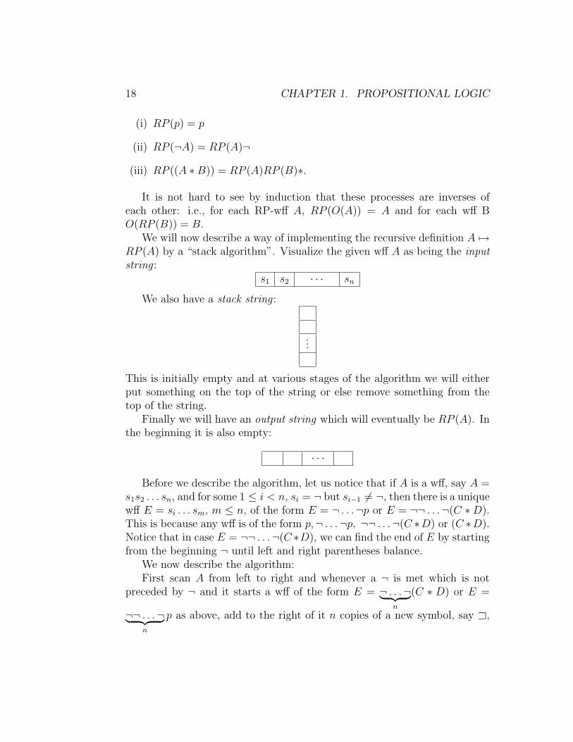
We will now describe a way of implementing the recursive definition A 7→RP (A) by a “stack algorithm”. Visualize the given wff A as being the inputstring :
s1 s2 · · · sn
We also have a stack string :
...
This is initially empty and at various stages of the algorithm we will eitherput something on the top of the string or else remove something from thetop of the string.
Finally we will have an output string which will eventually be RP (A). Inthe beginning it is also empty:
· · ·
Before we describe the algorithm, let us notice that if A is a wff, say A =s1s2 . . . sn, and for some 1 ≤ i < n, si = ¬ but si−1 6= ¬, then there is a uniquewff E = si . . . sm, m ≤ n, of the form E = ¬ . . .¬p or E = ¬¬ . . .¬(C ∗D).This is because any wff is of the form p,¬ . . .¬p, ¬¬ . . .¬(C ∗D) or (C ∗D).Notice that in case E = ¬¬ . . .¬(C ∗D), we can find the end of E by startingfrom the beginning ¬ until left and right parentheses balance.
We now describe the algorithm:First scan A from left to right and whenever a ¬ is met which is not
preceded by ¬ and it starts a wff of the form E = ¬ . . .¬︸ ︷︷ ︸n
(C ∗ D) or E =
¬¬ . . .¬︸ ︷︷ ︸n
p as above, add to the right of it n copies of a new symbol, say A,

1.3. POLISH AND REVERSE POLISH NOTATION 19
to obtain E AA · · · A︸ ︷︷ ︸n
. After this was done for all such occurrences of ¬ in
A we obtain a new string, say A′ (which might contain many occurrences ofthis new symbol A).
We now start scanning A′ from left to right. If we see ( do nothing.If we see p, we add p to the right of the output string. If we see ¬ or∗ ∈ {∧,∨,⇒,⇔}, we add this symbol to the top of the stack. If we see )or A we remove the top symbol in the stack and add it to the right of theoutput string. When we have scanned all of A′ this process stops and theoutput string is RP (A).
Example 1.3.8 Consider the wff
((s ⇒ ¬t) ⇒ ¬(p ∨ ¬(¬q ∧ s))) = A
for which the RP -wff is
st¬ ⇒ pq¬s ∧ ¬ ∨ ¬ ⇒= RP (A)
.
First we form A′:
((s ⇒ ¬t A) ⇒ ¬(p ∨ ¬(¬q A ∧s) A) A)
In the stack below, we represent top to bottom as right to left. Thereforethe top of the stack, where we push and pop symbols, is on the right.
input stack output( − −( − −s − s⇒ ⇒ s¬ ⇒ ¬ st ⇒ ¬ stA ⇒ st¬) − st¬ ⇒⇒ ⇒ st¬ ⇒¬ ⇒ ¬ st¬ ⇒

20 CHAPTER 1. PROPOSITIONAL LOGIC
input stack output( ⇒ ¬ st¬ ⇒p ⇒ ¬ st¬ ⇒ p∨ ⇒ ¬∨ st¬ ⇒ p¬ ⇒ ¬ ∨ ¬ st¬ ⇒ p( ⇒ ¬∨ ¬ st¬ ⇒ p¬ ⇒ ¬ ∨ ¬¬ st¬ ⇒ pq ⇒ ¬∨ ¬¬ st¬ ⇒ pqA ⇒ ¬∨ ¬ st¬ ⇒ pq¬∧ ⇒ ¬ ∨ ¬∧ st¬ ⇒ pq¬s ⇒ ¬∨ ¬∧ st¬ ⇒ pq¬s) ⇒ ¬∨ ¬ st¬ ⇒ pq¬s∧A ⇒ ¬∨ st¬ ⇒ pq¬s ∧ ¬) ⇒ ¬ st¬ ⇒ pq¬s ∧ ¬∨A ⇒ st¬ ⇒ pq¬s ∧ ¬ ∨ ¬) − st¬ ⇒ pq¬s ∧ ¬ ∨ ¬ ⇒
We will now verify the correctness of this algorithm, by induction on theconstruction of formulas. We will show that if we start with A and thenconstruct A′ and apply this stack algorithm but with the stack containingsome string S (not necessarily empty) and the output some string T (notnecessarily empty), then we finish with the stack string S and output stringT RP (A), whereˆmeans concatenation.
This is obvious if A = p. Assume it holds for B and consider A = ¬B.Then notice that A′ = ¬B′ A. Starting the algorithm from A′ and stackstring S and output string T , we first add ¬ to the top of S. Then weperform the algorithm on B′ and stack string S¬, output T . This finishes byproducing stack string S¬ and output T RP (B). Then since the last symbolof A′ is A, we get stack string S and output string T RP (B)¬ = T RP (A).
Finally assume it holds for B, C and consider A = (B ∗ C). Then A′ =(B′ ∗ C ′). Starting the algorithm from A′ and stack string S, output T ,we first have (, which does nothing. Then we have the algorithm on B′
on stack string S, output T which produces T RP (B) and stack string S.Then ∗ is put on top of the stack and the algorithm is applied to C ′ withstack string S∗ and output T RP (B) to produce stack string S∗ and output

1.4. ABBREVIATIONS 21
T RP (B)RP (C). Finally we have ) which produces stack string S and outputT RP (B) RP (C)∗ = T RP (A). a
1.4 Abbreviations
Sometimes in practice, in order to avoid complicated notation, we adoptvarious abbreviations in writing wff, if they don’t cause any confusion.
For example, we usually omit outside parentheses: We often write A∧Binstead of (A ∧B) or (A ∧B) ∨ C instead of ((A ∧B) ∨ C), etc.
Also we adopt an order of preference between the binary connectives,namely
∧,∨,⇒,⇔where connectives from left to right bind closer, i.e., ∧ binds closer than∨,⇒,⇔; ∨ binds closer than ⇒,⇔; and ⇒ binds closer than ⇔. So if wewrite p∧ q∨ r we really mean ((p∧ q)∨ r) and if we write p ⇒ q∨ r we reallymean (p ⇒ (q ∨ r)), etc.
Finally, when we have repeated connectives, we always associate paren-theses to the left, so that if we write A∧B∧C we really mean ((A∧B)∧C),and if we write A ⇒ B ⇒ C ⇒ D we really mean (((A ⇒ B) ⇒ C) ⇒ D).
1.5 Semantics of Propositional Logic
We now want to ask the question, “When is a proposition true or false?”Specifically, if we know whether each atomic proposition is true or false,what is the truth value of a compound proposition? We will consider twotruth values: T or 1 (true), and F or 0 (false).
1.5.A Valuations
Definition 1.5.1 A truth assignment or valuation consists of a map
ν : {p1, p2, . . . } → {0, 1}
assigning to each propositional variable a truth value.
Given such a ν we can extend it in a unique way to assign an associatedtruth value ν∗(A) to every wff A, by the following recursive definition:

22 CHAPTER 1. PROPOSITIONAL LOGIC
(i) ν∗(p) = ν(p).
(ii) ν∗(¬A) = 1− ν∗(A).
(iii) For the binary connectives, the rules are:
ν∗((A ∧B)) =
1 if ν∗(A) = ν∗(B) = 1
0 otherwise
= ν∗(A) · ν∗(B)
ν∗((A ∨B)) =
1 if ν∗(A) = 1 or ν∗(B) = 1
0 if ν∗(A) = ν∗(B) = 0
= 1− (1− ν∗(A)) · (1− ν∗(B))
ν∗((A ⇒ B)) = ν∗((¬A ∨B))
=
0 if ν∗(A) = 1, ν∗(B) = 0,
1 otherwise
= 1− ν∗(A) · (1− ν∗(B))
ν∗((A ⇔ B)) =
1 if ν∗(A) = ν∗(B)
0 otherwise
= ν∗(A) · ν∗(B) + (1− ν∗(A)) · (1− ν∗(B))
For simplicity, we will write ν(A) instead of ν∗(A), if there is no dangerof confusion.
These rules can be also represented by the following truth tables :
A B ¬A A ∧B A ∨B A ⇒ B A ⇔ B0 0 1 0 0 1 10 1 1 0 1 1 01 0 0 0 1 0 01 1 0 1 1 1 1
Note the similarity with the truth tables presented in section 1.1. We are nowformalizing our intuitive sense of what the propositional connectives should“mean.”

1.5. SEMANTICS OF PROPOSITIONAL LOGIC 23
Definition 1.5.2 For each wff A, its support, supp(A), is the set of propo-sitional variables occurring in it.
Example 1.5.3
supp(((p ∧ q) ⇒ (¬r ∨ p))︸ ︷︷ ︸A
) = {p, q, r}. (∗)
Thus we have, by way of recursive definition,
supp(p) = {p}supp(¬A) = supp(A)
supp((A ∗B)) = supp(A) ∪ supp(B).
The following is easy to check:
Proposition 1.5.4 If supp(A) = {q1, . . . , qn} and ν is a valuation, thenν(A) depends only on ν(q1), . . . , ν(qn); i.e., if µ is a valuation, and µ(qi) =ν(qi) for i = 1, . . . , n, then µ(A) = ν(A).
For instance, in example 1.5.3 above, ν(A) depends only on ν(p), ν(q),and ν(r).
We can visualize the calculation of ν(A) in terms of the parse tree TA asfollows, where we illustrate the general idea by an example.
Example 1.5.5 Consider A = ((p ⇒ ¬q) ⇒ (q ∨ p)) and its parse tree. Letν(p) = 0, ν(q) = 1. Then we can find the truth value of each node of thetree working upwards. So ν(A) = 1.
p (0)
q (1)
¬¬q (0)
p ⇒ ¬q (1)
⇒q (1) p (0)
q ∨ p (1)
∨
A (1)
⇒

24 CHAPTER 1. PROPOSITIONAL LOGIC
We also have the following algorithm for evaluating ν(A), given the val-uation ν to all the propositional variables in the support of A.
Algorithm 1.5.6 First replace each propositional variable p in A by itstruth value (according to ν), ν(p). Then scanning from left to right find thefirst occurence of a string of the form ¬i, (i ∧ j), (i ∨ j), (i ⇒ j), (i ⇔ j),where i, j ∈ {0, 1}, and replace it by its value according to the truth table(e.g., replace ¬0 by 1, (0 ∧ 1) by 0, etc.). Repeat the process until the valueν(A) is obtained.
Example 1.5.7 A, ν as in example 1.5.5. Then we first obtain ((0 ⇒ ¬1) ⇒(1∨ 0)). Next we have successively ((0 ⇒ 0) ⇒ (1∨ 0)), (1 ⇒ (1∨ 0)), (1 ⇒1), 1 = ν(A).
It is not hard to prove by induction on A that this algorithm is correct,i.e., produces always ν(A).
Given a valuation ν we can of course define in a similar way the truthvalue ν(A) for any P-wff or RP-wff A. We will now describe a stack algorithmfor calculating the truth value for RP-wff.
Algorithm 1.5.8 We start with a RP-wff A and a valuation ν to all thepropositional variables in the support of A. The stack is empty in the begin-ning.
We scan A from left to right. If we see a propositional variable p, we addto the top of the stack ν(p). If we see ¬, we replace the top of the stack a(which is either 0 or 1) by 1− a. If we see ∗ ∈ {∧,∨,⇒,⇔}, we replace thetop two elements of the stack b (= top), a (= next to top) by the value givenby the truth table for ∗ applied to the truth values a, b (in that order). Thetruth value in the stack, when we finish scanning A, is ν(A).
Example 1.5.9 Let A be the RP-wff
pqp¬∨ ⇒ rs¬u ⇒ ∨ ⇒ .
(in ordinary notation this is (p ⇒ (q ∨ ¬p)) ⇒ (r ∨ (¬s ⇒ u)) and ν(p) =1, ν(q) = 1, ν(r) = 0, ν(s) = 1, ν(u) = 1. Then by applying the algorithmwe have (once again, top to bottom on the stack is represented as right toleft):

1.5. SEMANTICS OF PROPOSITIONAL LOGIC 25
input stackp 1q 11p 111¬ 110∨ 11⇒ 1r 10s 101¬ 100u 1001⇒ 101∨ 11⇒ 1
Again it is easy to show by induction that this algorithm is correct, i.e.,it always produces ν(A). The appropriate statement we must prove, byinduction on the construction of A, is that if we start this algorithm withinput a RP-wff A and stack S, we end up by having stack Sν(A). (Here Sis a string of 0’s and 1’s.)
1.5.B Models and Tautologies
Definition 1.5.10 If ν is a valuation and A a wff, we say that ν satisfies ormodels A if ν(A) = 1.
That is, ν models A if A is true under the truth values that ν assigns tothe propositional variables. We use the notation
ν |= A
to denote that ν models A. We also write
ν 6|= A
26 CHAPTER 1. PROPOSITIONAL LOGIC
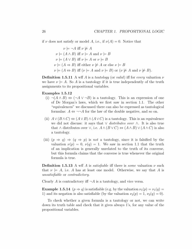
if ν does not satisfy or model A, i.e., if ν(A) = 0. Notice that
ν |= ¬A iff ν 6|= A
ν |= (A ∧B) iff ν |= A and ν |= B
ν |= (A ∨B) iff ν |= A or ν |= B
ν |= (A ⇒ B) iff either ν 6|= A or else ν |= B
ν |= (A ⇔ B) iff (ν |= A and ν |= B) or (ν 6|= A and ν 6|= B).
Definition 1.5.11 A wff A is a tautology (or valid) iff for every valuation νwe have ν |= A. So A is a tautology if it is true independently of the truthassignments to its propositional variables.
Examples 1.5.12(i) ¬(A ∧ B) ⇔ (¬A ∨ ¬B) is a tautology. This is an expression of one
of De Morgan’s laws, which we first saw in section 1.1. The other“equivalences” we discussed there can also be expressed as tautologicalformulas: A ⇔ ¬¬A for the law of the double negative, and so on.
(ii) A∨ (B ∧C) ⇔ (A∨B)∧ (A∨C) is a tautology. This is an equivalencewe did not discuss: it says that ∨ distributes over ∧. It is also truethat ∧ distributes over ∨, i.e. A∧ (B ∨C) ⇔ (A∧B)∨ (A∧C) is alsoa tautology.
(iii) (p ⇒ q) ⇒ (q ⇒ p) is not a tautology, since it is falsified by thevaluation ν(p) = 0, ν(q) = 1. We saw in section 1.1 that the truthof an implication is generally unrelated to the truth of its converse,but this formula claims that the converse is true whenever the originalformula is true.
Definition 1.5.13 A wff A is satisfiable iff there is some valuation ν suchthat ν |= A, i.e. A has at least one model. Otherwise, we say that A isunsatisfiable or contradictory.
Clearly A is contradictory iff ¬A is a tautology, and vice versa.
Example 1.5.14 (p ⇒ q) is satisfiable (e.g. by the valuation ν1(p) = ν1(q) =1) and its negation is also satisfiable (by the valuation ν2(p) = 1, ν2(q) = 0).
To check whether a given formula is a tautology or not, we can writedown its truth table and check that it gives always 1’s, for any value of thepropositional variables.

1.5. SEMANTICS OF PROPOSITIONAL LOGIC 27
Example 1.5.15 Consider (p ⇒ q) ⇔ (¬q ⇒ ¬p).
p q ¬p ¬q p ⇒ q ¬q ⇒ ¬p (p ⇒ q) ⇔ (¬q ⇒ ¬p)0 1 1 0 1 1 10 0 1 1 1 1 11 1 0 0 1 1 11 0 0 1 0 0 1
This procedure requires 2n many entries if the wff A contains n proposi-tional variables, so it has “exponential complexity.” No substantially moreefficient algorithm is known. The possibility of improving the “exponential”to “polynomial” complexity is a famous open problem in theoretical com-puter science known as the “P = NP problem”, that we will discuss inChapter 3.
We can extend the definition of satisfiability to sets containing more thanone formula. Clearly the only interesting notion is that of simultaneoussatisfiability; i.e. whether all formulas are satisfied by the same valuation.
Definition 1.5.16 If S is any set of wff (finite or infinite) and ν is a valua-tion, we say that ν satisfies or models S, in symbols
ν |= S
if ν |= A for every A ∈ S, i.e., ν models all wff in S. If there is somevaluation satisfying S we say that S is satisfiable (or has a model).
Examples 1.5.17(i) S = {(p1 ∨ p2), (¬p2 ∨ ¬p3), (p3 ∨ p4), (¬p4 ∨ ¬p5), . . . } is satisfiable,
with model the valuation:
ν(pi) =
{1 if i is odd;
0 if i is even.
(ii) S = {q ⇒ r, r ⇒ p, ¬p, q} is not satisfiable.
(iii) If S = {A1, . . . , An} is finite, then S is satisfiable iff A1 ∧ · · · ∧ An issatisfiable.

28 CHAPTER 1. PROPOSITIONAL LOGIC
1.5.C Logical Implication and Equivalence
Definition 1.5.18 Let now S be any set of wff and A a wff. (View S asa set of hypotheses and A as a conclusion.) We say that S (tauto)logicallyimplies A if every valuation that satisfies S satisfies also A (i.e., any modelof S is also a model of A).
If S logically implies A, we write
S |= A
(and if it does not, S 6|= A). We use the same symbol as for models of aformula, because the notions are compatible. If S = ∅, we just write |= A.This simply means that A is a tautology (it is true in all valuations).
Examples 1.5.19(i) (Modus Ponens) {A,A ⇒ B} |= B.
(ii) {A, A ⇒ (B ∨ C), B ⇒ D, C ⇒ D} |= D.
(iii) p ⇒ q 6|= q ⇒ p
(iv) {p1 ⇒ p2, p2 ⇒ p3, p3 ⇒ p4, . . . } |= p1 ⇒ pn (for any n)
(v) If S = {A1, . . . , An} is finite, then S = {A1, . . . , An} |= A iff A1 ∧ · · · ∧An |= A iff |= (A1 ∧ · · · ∧ An) ⇒ A.
(vi) S |= (A ⇒ B) iff S ∪ {A} |= B.
(vii) S |= A iff S ∪ {¬A} is not satisfiable.
Example 1.5.20 Consider the following argument (from Mendelson’s book“Introduction to Mathematical Logic”)
If capital investment remains constant, then government spend-ing will increase or unemployment will result. If governmentspending will not increase, taxes can be reduced. If taxes canbe reduced and capital investment remains constant, then un-employment will not result. Hence, government spending willincrease.
To see whether this conclusion logically follows from the premises, represent:

1.5. SEMANTICS OF PROPOSITIONAL LOGIC 29
p : “capital investment remains constant”q : “government spending will increase”r : “unemployment will result”s : “taxes can be reduced”
Then our premises are
S = {p ⇒ (q ∨ r), ¬q ⇒ s, s ∧ p ⇒ ¬r}
Our conclusion isA = q.
So we are asking ifS |= q.
This is false since the truth assignment ν(p) = 0, ν(q) = 0, ν(r) = 1, ν(s) = 1makes S true but q false. So the argument above is not valid.
Remark. Note that if S ⊆ S and S |= A, then S |= A. Also, if S |= A forall A ∈ S ′, and S ′ |= B, then S |= B.
Definition 1.5.21 Two wff A,B are called (logically) equivalent, in symbols
A ≡ B,
if A |= B and B |= A, i.e. A ⇔ B is a tautology.
Notice that logical equivalence is an equivalence relation, i.e.,
A ≡ A
A ≡ B implies B ≡ A
A ≡ B, B ≡ C imply A ≡ C.
We consider equivalent wff as semantically indistinguishable. However, ingeneral equivalent formulas are different syntactically. By that we mean thatthey are distinct strings of symbols, e.g. (p ⇒ q) and (¬q ⇒ ¬p).
Once again, we see the same equivalences that we mentioned in sec-tion 1.1, such as A ≡ ¬¬A and ¬(A ∧ B) ≡ (¬A ∨ ¬B). Here are a couplemore:
Examples 1.5.22(i) (A ⇔ B) ≡ ((A ∧B) ∨ (¬A ∧ ¬B))

30 CHAPTER 1. PROPOSITIONAL LOGIC
(ii) ((A ∧B) ⇒ C) ≡ ((A ⇒ C) ∨ (B ⇒ C))
Recommendation. Read Appendix A, which lists various useful tautolo-gies and equivalences. Verify that they are indeed tautologies and equiva-lences. You will often need to use some of them in homework assignments.
Here are some useful facts about logical equivalence.
(i) Let A be a wff containing the propositional variables q1, . . . , qn, and letA1, . . . , An be arbitrary wff. If A is a tautology, so is
A[q1/A1, q2/A2, . . . , qn/An],
the wff obtained by substituting qi by Ai (1 ≤ i ≤ n) in A.
(ii) If A is a wff, B a subformula of A and B′ a wff such that B ≡ B′,and we obtain A′ from A by substituting B by B′, then A ≡ A′. Thiscan be easily proved by induction on the construction of A. Thus wecan freely substitute equivalent formulas (as parts of bigger formulas)without affecting the truth value.
Example. A = (¬(p∧q) ⇒ (q∨r)), B = ¬(p∧q), B′ = (¬p∨¬q), A′ =((¬p ∨ ¬q) ⇒ (q ∨ r)).
The De Morgan Laws, which we have seen before, are the equivalences
¬(p ∧ q) ≡ (¬p ∨ ¬q)
¬(p ∨ q) ≡ (¬p ∧ ¬q)
By the first fact above, we can conclude that ¬(A ∧ B) ≡ (¬A ∨ ¬B),¬(A∨B) ≡ (¬A∧¬B) for any wff A,B. The De Morgan laws also have thefollowing generalization:
Proposition 1.5.23 (General De Morgan Laws) Let A be a wff cont-aining only the connectives ¬,∧,∨. Let A∗ be obtained from A by substitutingeach propositional variable p occurring in A by ¬p and replacing ∧ by ∨ and∨ by ∧. Then
¬A ≡ A∗.

1.6. TRUTH FUNCTIONS 31
Example 1.5.24
¬((p ∧ q) ∨ (¬r ∧ p)) ≡ ((¬p ∨ ¬q) ∧ (¬¬r ∨ ¬p))
≡ ((¬p ∨ ¬q) ∧ (r ∨ ¬p)), since ¬¬r ≡ r.
Proof. The proof of the General De Morgan’s Laws will be left for Home-work Assignment #2.
Augustus de Morgan was born in 1806 in Madura, India, and died in 1871in London. De Morgan lost the sight on his right eye as a boy. His familymoved to England when he was 10. At 1823, he refused to take a theologicaltest, and as a result Trinity College (Cambridge) only gave him a BA insteadof an MA. In 1828 he was appointed Professor at the new University College(London); he was the first mathematics professor of the college. De Morganwas first to formally define mathematical induction (1838). He was a friendof Charles Babbage, the creator of the first “difference engine” (1819–22), apredecessor of the modern computer. This led to his interest in logic as analgebra of identities and to his introduction of what are now known as DeMorgan’s laws.
“A dry dogmatic pedant I fear is Mr. De Morgan, notwithstanding hisunquestioned ability.” Thomas Hirst.
1.6 Truth Functions
We can consider a formula (or even an equivalence class of logically equiv-alent formulas) to define a function. Its inputs are the truth values of thepropositional variables in its support (that is, a valuation, or at least therelevant part of a valuation), and its output is the truth value of the formula(that is, whether the valuation models the formula). We can also go theother way: starting from any such function, we will construct a propositionalformula which describes it.
1.6.A Truth Functions
Definition 1.6.1 For n ≥ 1, an n-ary truth function (also called a Booleanfunction) is any map
f : {0, 1}n → {0, 1}.
32 CHAPTER 1. PROPOSITIONAL LOGIC
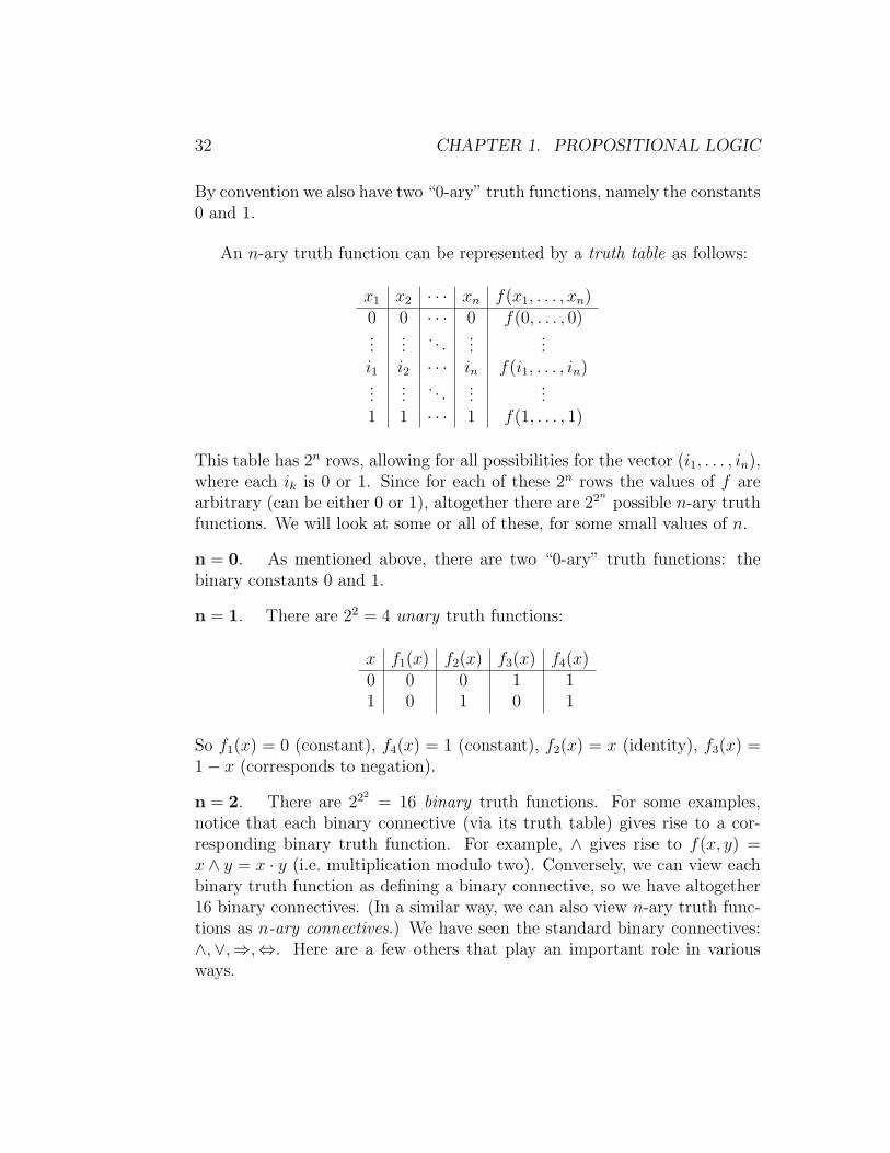
By convention we also have two “0-ary” truth functions, namely the constants0 and 1.
An n-ary truth function can be represented by a truth table as follows:
x1 x2 · · · xn f(x1, . . . , xn)0 0 · · · 0 f(0, . . . , 0)...
.... . .
......
i1 i2 · · · in f(i1, . . . , in)...
.... . .
......
1 1 · · · 1 f(1, . . . , 1)
This table has 2n rows, allowing for all possibilities for the vector (i1, . . . , in),where each ik is 0 or 1. Since for each of these 2n rows the values of f arearbitrary (can be either 0 or 1), altogether there are 22n
possible n-ary truthfunctions. We will look at some or all of these, for some small values of n.
n = 0. As mentioned above, there are two “0-ary” truth functions: thebinary constants 0 and 1.
n = 1. There are 22 = 4 unary truth functions:
x f1(x) f2(x) f3(x) f4(x)0 0 0 1 11 0 1 0 1
So f1(x) = 0 (constant), f4(x) = 1 (constant), f2(x) = x (identity), f3(x) =1− x (corresponds to negation).
n = 2. There are 222= 16 binary truth functions. For some examples,
notice that each binary connective (via its truth table) gives rise to a cor-responding binary truth function. For example, ∧ gives rise to f(x, y) =x ∧ y = x · y (i.e. multiplication modulo two). Conversely, we can view eachbinary truth function as defining a binary connective, so we have altogether16 binary connectives. (In a similar way, we can also view n-ary truth func-tions as n-ary connectives.) We have seen the standard binary connectives:∧,∨,⇒,⇔. Here are a few others that play an important role in variousways.
1.6. TRUTH FUNCTIONS 33
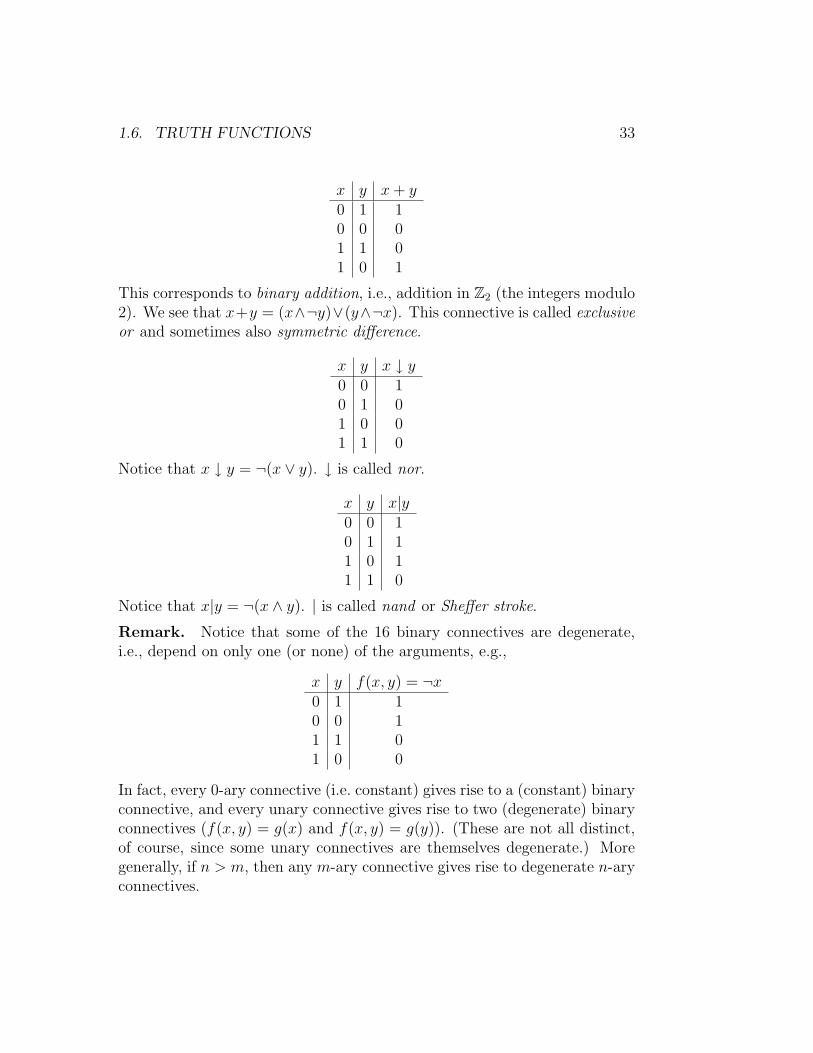
x y x + y0 1 10 0 01 1 01 0 1
This corresponds to binary addition, i.e., addition in Z2 (the integers modulo2). We see that x+y = (x∧¬y)∨(y∧¬x). This connective is called exclusiveor and sometimes also symmetric difference.
x y x ↓ y0 0 10 1 01 0 01 1 0
Notice that x ↓ y = ¬(x ∨ y). ↓ is called nor.
x y x|y0 0 10 1 11 0 11 1 0
Notice that x|y = ¬(x ∧ y). | is called nand or Sheffer stroke.
Remark. Notice that some of the 16 binary connectives are degenerate,i.e., depend on only one (or none) of the arguments, e.g.,
x y f(x, y) = ¬x0 1 10 0 11 1 01 0 0
In fact, every 0-ary connective (i.e. constant) gives rise to a (constant) binaryconnective, and every unary connective gives rise to two (degenerate) binaryconnectives (f(x, y) = g(x) and f(x, y) = g(y)). (These are not all distinct,of course, since some unary connectives are themselves degenerate.) Moregenerally, if n > m, then any m-ary connective gives rise to degenerate n-aryconnectives.
34 CHAPTER 1. PROPOSITIONAL LOGIC
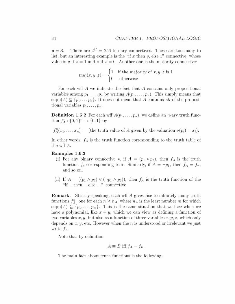
n = 3. There are 223= 256 ternary connectives. These are too many to
list, but an interesting example is the “if x then y, else z” connective, whosevalue is y if x = 1 and z if x = 0. Another one is the majority connective:
maj(x, y, z) =
{1 if the majority of x, y, z is 1
0 otherwise
For each wff A we indicate the fact that A contains only propositionalvariables among p1, . . . , pn by writing A(p1, . . . , pn). This simply means thatsupp(A) ⊆ {p1, . . . pn}. It does not mean that A contains all of the proposi-tional variables p1, . . . , pn.
Definition 1.6.2 For each wff A(p1, . . . , pn), we define an n-ary truth func-tion fn
A : {0, 1}n → {0, 1} by
fnA(x1, . . . , xn) = (the truth value of A given by the valuation ν(pi) = xi).
In other words, fA is the truth function corresponding to the truth table ofthe wff A.
Examples 1.6.3(i) For any binary connective ∗, if A = (p1 ∗ p2), then fA is the truth
function f∗ corresponding to ∗. Similarly, if A = ¬p1, then fA = f¬,and so on.
(ii) If A = ((p1 ∧ p2) ∨ (¬p1 ∧ p3)), then fA is the truth function of the“if. . . then. . . else. . . ” connective.
Remark. Strictly speaking, each wff A gives rise to infinitely many truthfunctions fn
A: one for each n ≥ nA, where nA is the least number m for whichsupp(A) ⊆ {p1, . . . , pm}. This is the same situation that we face when wehave a polynomial, like x + y, which we can view as defining a function oftwo variables x, y, but also as a function of three variables x, y, z, which onlydepends on x, y, etc. However when the n is understood or irrelevant we justwrite fA.
Note that by definition
A ≡ B iff fA = fB.
The main fact about truth functions is the following:
1.6. TRUTH FUNCTIONS 35
Theorem 1.6.4 Every truth function is realized by a wff containing only¬,∧,∨. That is, if f : {0, 1}n → {0, 1} with n ≥ 1, there is a wff
A(p1, . . . , pn)
containing only ¬,∧,∨ such that
f = fA (= fnA).
Proof. If f is identically 0, take A = (p1 ∧ ¬p1).Otherwise, for each entry s = (x1, . . . , xn) ∈ {0, 1}n in the truth table of
f , introduce the wff
As = ε1p1 ∧ ε2p2 ∧ · · · ∧ εnpn
where
εi =
{nothing if xi = 1
¬ if xi = 0.
Example. s = (1, 0, 1) → As = p1 ∧ ¬p2 ∧ p3.Notice that fAs(x1, . . . , xn) = 1, but fAs(x
′1, . . . , x
′n) = 0 if (x′1, . . . , x
′n) 6=
(x1, . . . , xn). Enumerate in a sequence s1, . . . , sm (m ≤ 2n) all s ∈ {0, 1}n
such that f(s) = 1 (and there is at least one such) and put
A = As1 ∨ As2 ∨ · · · ∨ Asm .
Then fA(s) = 1 iff at least one of fAsi(s) = 1 iff s ∈ {s1, . . . , sm} iff f(s) = 1,
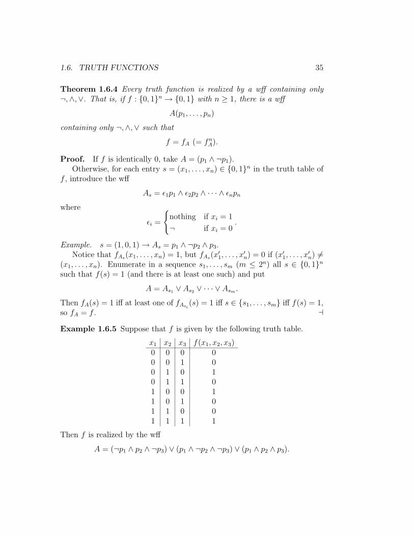
so fA = f . aExample 1.6.5 Suppose that f is given by the following truth table.
x1 x2 x3 f(x1, x2, x3)0 0 0 00 0 1 00 1 0 10 1 1 01 0 0 11 0 1 01 1 0 01 1 1 1
Then f is realized by the wff
A = (¬p1 ∧ p2 ∧ ¬p3) ∨ (p1 ∧ ¬p2 ∧ ¬p3) ∨ (p1 ∧ p2 ∧ p3).

36 CHAPTER 1. PROPOSITIONAL LOGIC
Corollary 1.6.6 Any wff is equivalent to a wff containing only ¬,∧ and toa wff containing only ¬,∨. So any truth function can be realized by a wffcontaining only ¬,∧ or only ¬,∨.
Proof. Given a wff A(p1, . . . , pn), consider the truth function fA : {0, 1}n →{0, 1} and let A′(p1, . . . , pn) be a wff containing only ¬,∧,∨ such that
fA = fA′ ,
i.e.A ≡ A′.
We can now systematically eliminate ∨ by using the equivalence
C ∨D ≡ ¬(¬C ∧ ¬D) (1.1)
to obtain an equivalent formula A′′ ≡ A′ containing only ¬,∧. Similarlyusing
C ∧D ≡ ¬(¬C ∨ ¬D) (1.2)
we can find an equivalent formula A′′′ ≡ A′ containing only ¬,∨. aRemark. Another way to prove this corollary is by using the equivalences(1.1) and (1.2) above, as well as
(C ⇒ D) ≡ (¬C ∨D)
(C ⇔ D) ≡ (¬C ∨D) ∧ (¬D ∨ C)
to systematically eliminate all connectives except ¬,∨ or ¬,∧.
Example 1.6.7 Suppose A is
((p ⇒ q) ∧ ¬(r ⇒ s)) ∨ (s ∨ p),
and we want to find an equivalent wff involving only ¬,∧. We have thefollowing equivalent wffs, successively:
((p ⇒ q) ∧ ¬(r ⇒ s)) ∨ (s ∨ p) = A,
((¬p ∨ q) ∧ ¬(¬r ∨ s)) ∨ (s ∨ p),
(¬(p ∧ ¬q) ∧ (r ∧ ¬s)) ∨ ¬(¬s ∧ ¬p),
¬(¬(¬(p ∧ ¬q) ∧ (r ∧ ¬s))) ∧ (¬s ∧ ¬p)).
1.6. TRUTH FUNCTIONS 37
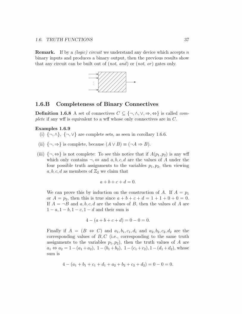
Remark. If by a (logic) circuit we understand any device which accepts nbinary inputs and produces a binary output, then the previous results showthat any circuit can be built out of (not, and) or (not, or) gates only.
--
-
-
1.6.B Completeness of Binary Connectives
Definition 1.6.8 A set of connectives C ⊆ {¬,∧,∨,⇒,⇔} is called com-plete if any wff is equivalent to a wff whose only connectives are in C.
Examples 1.6.9(i) {¬,∧}, {¬,∨} are complete sets, as seen in corollary 1.6.6.
(ii) {¬,⇒} is complete, because (A ∨B) ≡ (¬A ⇒ B).
(iii) {¬,⇔} is not complete: To see this notice that if A(p1, p2) is any wffwhich only contains ¬,⇔ and a, b, c, d are the values of A under thefour possible truth assignments to the variables p1, p2, then viewinga, b, c, d as members of Z2 we claim that
a + b + c + d = 0.
We can prove this by induction on the construction of A. If A = p1
or A = p2, then this is true since a + b + c + d = 1 + 1 + 0 + 0 = 0.If A = ¬B and a, b, c, d are the values of B, then the values of A are1− a, 1− b, 1− c, 1− d and their sum is
4− (a + b + c + d) = 0− 0 = 0.
Finally if A = (B ⇔ C) and a1, b1, c1, d1 and a2, b2, c2, d2 are thecorresponding values of B, C (i.e., corresponding to the same truthassignments to the variables p1, p2), then the truth values of A area1 ⇔ a2 = 1− (a1 +a2), 1− (b1 + b2), 1− (c1 + c2), 1− (d1 +d2), whosesum is
4− (a1 + b1 + c1 + d1 + a2 + b2 + c2 + d2) = 0− 0 = 0.

38 CHAPTER 1. PROPOSITIONAL LOGIC
Since the values of p1 ∧ p2 are 1, 0, 0, 0 whose sum is 1, it follows thatp1∧p2 cannot be equivalent to any wff built using only ¬,⇔, so {¬,⇔}is not complete.
Recall that we actually have 16 binary connectives. We can introduce asymbol for each one of them (as we have already done for the most commonones) and build up formulas using them. So we can generalize the precedingdefinition to say that any set C of binary connectives is complete if any wffis equivalent to one in which the only connectives are contained in C. (Interms of truth functions this simply means that every truth function can beexpressed as a composition of the truth functions contained in C. To see thisnotice that if ∗ is a binary connective, then fA∗B(x) = ∗(fA(x), fB(x)).)
A single binary connective ∗ is complete if C = {∗} is complete, i.e., everywff is equivalent to one using only ∗. It turns out that the nand (|), and nor(↓) connectives are complete. This is easily seen, because
¬p ≡ p|p ≡ p ↓ p
(p ∨ q) ≡ (p|p)|(q|q)(p ∧ q) ≡ (p ↓ p) ↓ (q ↓ q).
We will see in Assignment #3 that these are the only complete binary con-nectives.
Remark. In terms of circuits this implies that they can all be built usingonly nor or nand gates:
nand gate nor gate
-
--
-
--
1.6.C Normal Forms
Definition 1.6.10 A wff A is in disjunctive normal form (dnf ) if
A = A1 ∨ · · · ∨ An,
withAi = `
(i)1 ∧ · · · ∧ `
(i)ki
,
and each `(i)j a literal, i.e., p or ¬p for some propositional variable p. We call
Ai the disjuncts of A.

1.6. TRUTH FUNCTIONS 39
Examples 1.6.11(i) p, p ∧ q, (p ∧ q) ∨ (¬r ∧ s), p ∨ ¬q ∨ (s ∧ ¬t ∧ u) are in dnf.
(ii) p ⇒ q and (p ∨ (q ∧ r)) ∧ s are not in dnf.
Theorem 1.6.12 For every wff A we can find a wff B in dnf such thatA ≡ B.
Proof. This follows from the proof of Theorem 1.6.4. If A = A(p1, . . . , pn)and A is contradictory, take B = p1 ∧ ¬p1. Otherwise, let
X = {(ε1, . . . , εn) : the truth assigment pi 7→ εi satisfies A} ⊆ {0, 1}n,
and let
B =∨
(ε1,...,εn)∈X
n∧i=1
εipi,
where εipi = pi if ε1 = 1 and ¬pi if εi = 0. (The notation∧n
i=1, like∑n
i=1,means to connect the specified values with ∧, as i runs from 1 to n.) ThenB is the desired formula. a
Definition 1.6.13 A wff A is in conjunctive normal form (cnf) iff
A = A1 ∧ · · · ∧ An,
withAi = `
(i)1 ∨ · · · ∨ `
(i)ki
and each `(i)j a literal. We call Ai the conjuncts of A.
Example 1.6.14
p, p ∨ q, (p ∨ q) ∧ (¬r ∨ s), p ∧ ¬q ∧ (s ∨ ¬t ∨ u) are in cnf.
p ⇒ q, (p ∨ (q ∧ r)) ∧ s, and (p ∧ q) ∨ r are not in cnf.
Corollary 1.6.15 For every wff A we can find a wff B in cnf such thatA ≡ B.
Proof. Apply the preceding theorem to ¬A to find a wff B′ in dnf suchthat
¬A ≡ B′,

40 CHAPTER 1. PROPOSITIONAL LOGIC
so
A ≡ ¬B′.
Now
B′ =n∨
i=1
ki∧j=1
`(i)j ,
so, by de Morgan,
¬B′ ≡n∧
i=1
ki∨j=1
¬`(i)j .
If some `(i)j is of the form ¬p replace ¬`
(i)j by p to obtain ˜(i)
j . Otherwise let˜(i)j = `
(i)j . Thus
¬B′ ≡n∧
i=1
ki∨j=1
˜(i)j = B,
where each ˜(i)j is a literal, so B is in cnf and A ≡ B. a
Remark. Given a wff A in dnf it is easy to check if it is satisfiable or not:If
A =n∨
i=1
ki∧j=1
`(i)j ,
then A is satisfiable iff one of the disjuncts is satisfiable, which is true iff thereis 1 ≤ i ≤ n so that {`(i)
j : 1 ≤ j ≤ ki) does not contain both a propositionalvariable and its negation. Similarly given a wff A in cnf, it is easy to check ifit is a tautology or not: it is a tautology iff all the conjuncts are tautologies,which happens iff for all 1 ≤ i ≤ n, {`(i)
j : 1 ≤ i ≤ ki} contains both apropositional variable and its negation.
Examples 1.6.16(i) (p ∧ q) ∨ (p ∧ ¬r ∧ s) ∨ (p ∧ s ∧ ¬p) is satisfiable.
(ii) (p ∨ q) ∧ (r ∨ s ∨ ¬r) ∧ (t ∨ p ∨ ¬s ∨ ¬t) is not a tautology.
This is one reason that cnf and dnf are useful forms to be able to put awff in. However it is not known how to transform efficiently any given wff Ato an equivalent one in dnf (or cnf).
1.7. KONIG’S LEMMA AND APPLICATIONS 41
1.7 Konig’s Lemma and Applications
We will now temporarily take a break from propositional logic and discuss abasic result in combinatorics, which we will use in the next section to provean important result about propositional logic known as the CompactnessTheorem.
1.7.A Graphs and Trees
Definition 1.7.1 A (nondirected, simple) graph consists of a set of verticesV and a set E ⊆ V 2 of edges with the property that
(x, y) ∈ E iff (y, x) ∈ E,
(x, x) 6∈ E.
If e = (x, y) ∈ E is an edge, we say that x, y are adjacent.
We represent a graph geometrically by drawing points for vertices andconnecting adjacent vertices with lines, as shown.
x y
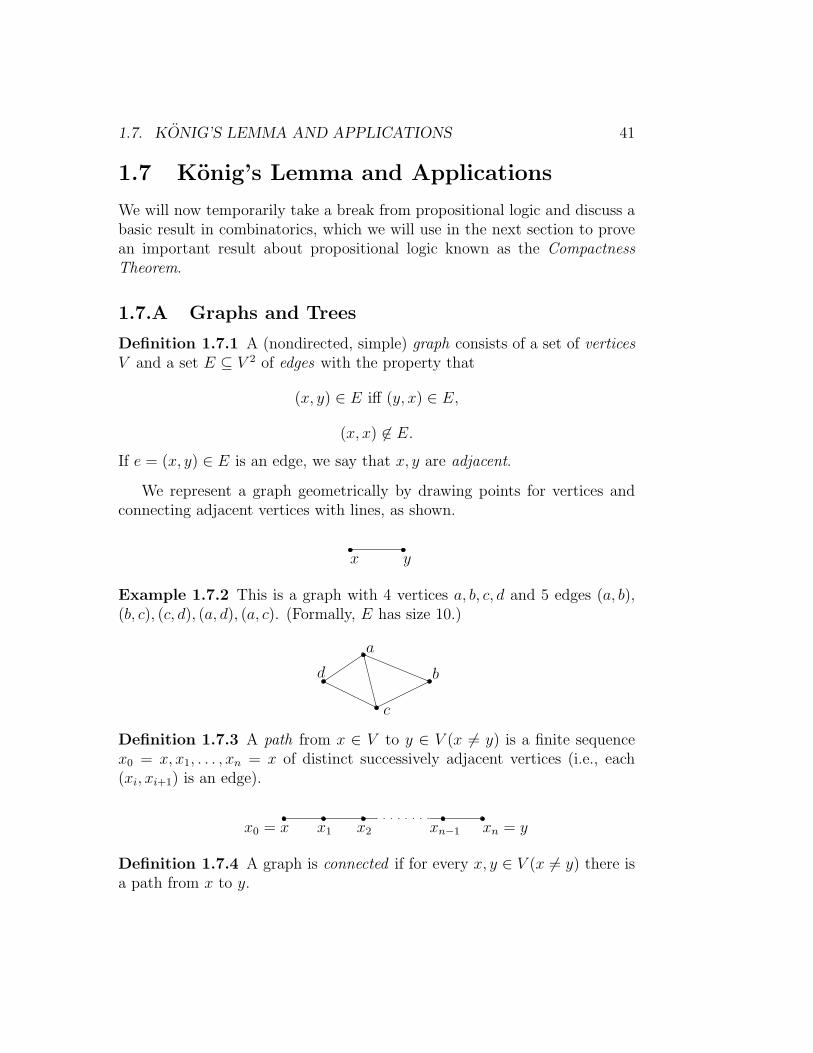
Example 1.7.2 This is a graph with 4 vertices a, b, c, d and 5 edges (a, b),(b, c), (c, d), (a, d), (a, c). (Formally, E has size 10.)
d
c
a
b
Definition 1.7.3 A path from x ∈ V to y ∈ V (x 6= y) is a finite sequencex0 = x, x1, . . . , xn = x of distinct successively adjacent vertices (i.e., each(xi, xi+1) is an edge).
x0 = x x1 x2 xn−1 xn = y
Definition 1.7.4 A graph is connected if for every x, y ∈ V (x 6= y) there isa path from x to y.

42 CHAPTER 1. PROPOSITIONAL LOGIC
Definition 1.7.5 A graph is a tree if for any x 6= y there is a unique pathfrom x to y.
Examples 1.7.6Here are some examples of graphs that are and are not trees.
not a tree tree not a tree(not connected) (has loops)
Equivalently, a connected graph is a tree exactly when it contains noloops (or cycles), where a loop is a sequence of successively adjacent verticesx0, x1, . . . , xn with x0 = xn and x0, . . . , xn−1 distinct.
Example 1.7.7 Here is a loop:
x0 = x5
x1
x2
x3
x4
Definition 1.7.8 A rooted tree is a tree with a distinguished vertex calledthe root.
The root is usually denoted by v0. For every vertex v 6= v0 there is aunique path v0, v1, . . . , vn = v.
v0
v1
v2
v3

1.7. KONIG’S LEMMA AND APPLICATIONS 43
Definition 1.7.9 The parent of v is the vertex vn−1 and the children of vare all the vertices v′ such that v0, v1, . . . , vn, vn+1 = v′ is the unique pathfrom v0 to v′.
parent of v
v
︸ ︷︷ ︸children of v
1.7.B Konig’s Lemma
Definition 1.7.10 A tree is finite splitting if every vertex has only finitelymany children (thus only finitely many adjacent vertices).
. . . . . .
finite splitting not finite splitting
Definition 1.7.11 An infinite branch of a rooted tree is an infinite sequencev0, v1, v2, . . . , where vn+1 is a child of vn.
v5...
v4
v3
v2
v1
v0

44 CHAPTER 1. PROPOSITIONAL LOGIC
For example, if T is the infinite binary tree (in which each vertex hasexactly two children), then the infinite branches correspond exactly to theinfinite binary sequences a1, a2, a3, a4, . . . (each ai = 0 or 1), where we inter-pret 0 as going left and 1 as going right.
......
00
......
01
0
......
10
......
11
1
Theorem 1.7.12 (Konig’s Lemma) If a finite splitting tree has infinitelymany vertices, then it has an infinite branch.
Note that this fails if the tree is not finite splitting. Consider the followingcounterexample:
. . .
Proof. Let T be the given tree. For each vertex v of the tree, let Tv bethe subtree of T consisting of v, the children of v, the grandchildren of v,etc., i.e., consisting of v and all its descendents, and all the edges connectingthem. Denote by V the set of vertices of T , and by Vv the set of vertices ofTv.
v
Tv
v0

1.7. KONIG’S LEMMA AND APPLICATIONS 45
We will use the following version of the Pigeon Hole Principle: If X is aninfinite set and X = X1 ∪ · · · ∪Xn, then some Xi, 1 ≤ i ≤ n, is infinite.
Now, since T is finite splitting, v0 has only finitely many children, sayc1, . . . , cn. Then V = {v0}∪Vc1∪· · ·∪Vcn , so some Vci1
is infinite. Put v1 = ci1 .Let then d1, . . . , dm be the children of v1. We have Vv1 = {v1}∪Vd1∪· · ·∪Vdm ,so one of the Vdi
, say Vdi2is infinite. Put v2 = di2 , etc. Proceeding this way,
we define an infinite path v0, v1, v2, . . . (so that for each n, Vvn is infinite).a
1.7.C Domino Tilings
As an application of Konig’s Lemma, we will consider the following tilingproblem in the plane.
Definition 1.7.13 A domino system consists of a finite set D of dominotypes, where a domino type is a unit square with each side labeled.
Examples 1.7.14Here are some example domino types:
ab
ac
ab
cd
10
23
Definition 1.7.15 A tiling of the plane by D consists of a filling-in of theplane by dominoes of type in D, so that adjacent dominoes have matchinglabels at the sides where they touch. (Dominoes cannot be rotated.)
Example 1.7.16 Here is a tiling of the plane:
bb
ac
ab
cd
cd
ba
cc
db
dd
bb
ba
cd
For this tiling, D contains at least
bb
ac
ab
cd
cd
ba
cc
db
dd
bb
ba
cd

46 CHAPTER 1. PROPOSITIONAL LOGIC
Problem. Given D, can one tile the plane by D?
Examples 1.7.17(i) Suppose D consists of
31
12
14
25
27
38
62
41
45
54
58
67
Then D can tile the plane, by repeating the following pattern:
31
12
14
25
27
38
62
41
45
54
58
67
(ii) Suppose, on the other hand, that D consists of
13
21
22
32
31
12
This D cannot tile the plane, as the following forced configurationshows:
13
21
22
32
31
12
13
21
Starting from the 13
21 on the right, we are forced to form this config-
uration, which cannot be completed to a tiling. Starting from 31
12 in
the middle, we are again forced to this configuration. Finally, starting
from 22
32 on the left we are again forced to this configuration.
We can similarly define what it means to tile a rectangular finite regionof the plane, like

1.7. KONIG’S LEMMA AND APPLICATIONS 47
or an infinite region, like
We just impose no restriction on the boundaries. Here is then a surprisingfact:
Theorem 1.7.18 For any given (finite) set D of domino types, D can tilethe plane iff D can tile the upper right quadrant.
Proof. We will actually show that the following are equivalent:
(i) D can tile the plane.
(ii) D can tile the upper right quadrant.
(iii) For each n = 1, 2, . . . , D can tile the n× n square.
It is clear that (i) implies (ii) implies (iii), so it is enough to show that (iii)implies (i).
So assume that for each n = 1, 2, . . . , D can tile the n × n square. Webuild a tree as follows:
The children of the root v0 are all possible tilings of the 1× 1 square, i.e.,all domino types in D. They are only finitely many. Let a be a typical oneof them. Then its children are all the tilings of the 3 × 3 square consistentwith a (viewed as being in the middle of the 3 × 3 square). Let b a typicalone of them. Then its children are the tilings of the 5× 5 square consistentwith b, etc.

48 CHAPTER 1. PROPOSITIONAL LOGIC
This tree is finite splitting, since for each fixed tiling of a (2n+1)×(2n+1)square there are only finitely many ways of extending it to a tiling of the (2n+3)× (2n + 3) square, since D is finite. The tree is also infinite, since for eachn ≥ 1 there is some tiling of the (2n−1)×(2n−1) square, say un, and if we letu1, u2, . . . un−1 be the tilings of the middle 1×1, 3×3, . . . , (2n−3)×(2n−3)squares contained in un, then u0, u1, . . . , un are all vertices in this tree, sofor each n the tree has at least n vertices, i.e., it is infinite. So by Konig’sLemma there is an infinite branch of the tree, say u0, u1, u2, . . . un, . . . Thisgives, in an obvious way, a tiling of the plane by D. aRemark. It can be proved that there is no algorithm to check whether agiven D can tile the plane or not.
This has the following interesting implication. A periodic tiling by Dconsists of a tiling of an (n×m)-rectangle, so that the top and bottom labelsmatch and so do the right and left ones, so by repeating it we can tile theplane.
Theorem 1.7.19 There is a domino system D which can tile the plane, buthas no periodic tiling.
Proof. If this fails, then for every D which can tile the plane, there is aperiodic tiling. Then we can devise an algorithm for checking whether a givenD can tile the plane or not, which is a contradiction. First enumerate, in somestandard way, all pairs (n,m), (n ≥ 1,m ≥ 1) (e.g. as shown in the figure),say (ni,mi), i = 1, 2, . . . Then generate all tilings of the (n1×m1)-rectangle,the (n2 ×m2)-rectangle (if any), etc.
1 2 3 4 51
2
3
4
-IjI
I
For each fixed (ni,mi) this is a finite process. Stop the process when some(ni,mi) is found for which either there is a periodic tiling of the (ni ×mi)-rectangle, or else there is no tiling of the (ni×mi)-rectangle. In the first case,D can tile the plane and in the second it cannot. The only thing left to prove
1.7. KONIG’S LEMMA AND APPLICATIONS 49
is that this process terminates, i.e. for some i this must happen. But this isthe case, since either D can tile the plane and so by our assumption there is aperiodic tiling (of some (ni×mi)-rectangle)) or else D cannot tile the plane,so, by the proof of Theorem 1.6.2, D cannot tile the (ni ×mi)-rectangle forsome ni = mi. a
1.7.D Compactness of [0, 1]
As another application, we will use Konig’s Lemma to prove that the unitinterval [0,1] is compact. This means the following: Let (ai, bi), i = 1, 2, . . .be a sequence of open intervals such that
[0, 1] ⊆⋃i
(ai, bi).
Then there are i1, . . . , ik such that
[0, 1] ⊆ (ai1 , bi1) ∪ · · · ∪ (aik , bik).
To prove this, consider the so-called dyadic intervals which are obtainedby successively splitting [0,1] in half. They can be pictured as a binary tree.
We will prove that there is an n such that every one of the dyadic intervalsat the nth level of the tree (i.e., those with denominators 2−n) is containedin some (ai, bi) (perhaps different (ai, bi) for different dyadic intervals). Thisproves what we want.
The proof is by contradiction: If this fails, then for each n there is somedyadic interval at the nth level which is not contained in any (ai, bi). Considerthen the subtree T of the tree of dyadic intervals, consisting of all vertices (i.e.,dyadic intervals) I which are not contained in any (ai, bi). Then for each n,there is an I = In at the n-th level belonging to T , and if I0 = [0, 1], I1, . . . , In
is the unique path from the root to In, it is clear that I0 ⊇ I1 ⊇ · · · ⊇ In,so no one of I0, I1, . . . , In are contained in any (ai, bi), so the tree T has atleast n vertices for each n, thus it is infinite. It is clearly finite splitting. Soby Konig’s Lemma, it has an infinite branch I0, I1, I2, . . . Then I0 ⊇ I1 ⊇I2 ⊇ . . . are closed intervals and the length of In is 2−n, so there is a uniquepoint x ∈ ⋂
n In. Since [0, 1] ⊆ ⋃i(ai, bi), for some i we have x ∈ (ai, bi), and
if n is large enough so that min{x − ai, bi − x} > 2−n, then In ⊆ (ai, bi), acontradiction.

50 CHAPTER 1. PROPOSITIONAL LOGIC
1.8 The Compactness Theorem
We now return to propositional logic. In this section we will prove a basicresult known as the Compactness Theorem and some applications of it.
1.8.A The Compactness Theorem
The compactness theorem has two equivalent versions.
Theorem 1.8.1 (Compactness Theorem I) Let S be any set of formulasin propositional logic. If every finite subset S0 ⊆ S is satisfiable, then S issatisfiable.
Theorem 1.8.2 (Compactness Theorem II) Let S be any set of formu-las in propositional logic, and A any formula. Then if S |= A, there is afinite subset S0 ⊆ S such that S0 |= A.
First we show that these two forms are equivalent.
I implies II. Assume I holds for any S. Fix then S and A with S |= A.Then S ′ = S ∪ {¬A} is not satisfiable, so, by applying I to S ′, we have afinite S ′0 ⊆ S ′ = S ∪ {A}, so that S ′0 is not satisfiable. Say S ′0 ⊆ S0 ∪ {¬A},with S0 ⊆ S finite. Then S0 ∪ {¬A} is not satisfiable, so S0 |= A.
II implies I. Say S is not satisfiable. Then S |=⊥, where ⊥= p ∧ ¬p. Soby II S0 |=⊥ for some finite S0 ⊆ S. Then S0 is unsatisfiable.
We will now prove form I of the Compactness Theorem.
Proof of 1.8.1. We assume that every finite subset S0 ⊆ S is satisfiable.We will then build a finite splitting tree which is infinite and thus, by Konig’sLemma, has an infinite branch. This infinite branch will give a truth assign-ment satisfying S.
First let us notice that we can enumerate in a sequence A1, A2, A3, . . . ,An, . . . all wff. So we can enumerate in a sequence
S = {B1, B2, B3, . . . , Bn, . . . }all wff in S. Next k1 < k2 < k3 < · · · < kn < . . . are chosen so that
Bn = Bn(p1, . . . , pkn)
i.e, all the propositional variables of Bn are among p1, . . . , pkn .

1.8. THE COMPACTNESS THEOREM 51
We will now build a tree as follows: Let v0 be the root. The childrenof v0 are all valuations v1 = (ε1, . . . , εk1) ∈ {0, 1}k1 which satisfy B1. Fixany such v1, say v1 = (ε1, . . . , εk1). Its children are all valuations v2 =(ε1, . . . , εk1 , εk1+1, . . . , εk2) ∈ {0, 1}k2 , which agree with v1 in their first k1
values and also satisfy both B1 and B2, etc.First we argue that this tree is infinite: Fix any n ≥ 1. By assumption
there is a valuation vn = {ε1, . . . , εkn} ∈ {0, 1}kn which satisfies {B1, . . . , Bn}.Let for 1 ≤ m ≤ n, vm = {ε1, . . . , εkm}, i.e., the restriction of vn to the firstkm variables. Then clearly vm satisfies {B1, . . . , Bm}, so it is a vertex of ourtree, and vm+1 is a child of vm. So T has at least n vertices for each n, i.e.,it is infinite. Clearly T is finite splitting. So, by Konig’s Lemma, it has aninfinite branch v0, v1, v2, . . . , vn, . . . Then
v1 = {ε1, . . . , εk1}v2 = {ε1, . . . , εk1 , εk1+1, . . . , εk2}
...
vn = {ε1, . . . , εk1 , εk1+1, . . . , εk2 , εk2+1, . . . , εkn}...
So if ν = {ε1, ε2, . . . }, ν is a valuation which satisfies all the Bn, i.e., itsatisfies S, and so S is satisfiable. a
1.8.B A Proof of Konig’s Lemma
We have proved the Compactness Theorem by using Konig’s Lemma. Onthe other hand, we can also prove Konig’s Lemma by using the CompactnessTheorem as follows:
Consider a tree T with root v0 which is infinite, but has finite splitting.Notice then that the set V of the vertices of T can be enumerated in asequence. Introduce now a propositional variable pv for each vertex v of T .(Our preceding remark implies that we can enumerate these variables in asequence p1, p2, . . . , but there is no point in doing that explicitly.) Considernow the following set S of wff, which we can view as “axioms”, where theintuitive meaning of the variable pv is that “pv is true” iff “v is in the infinitebranch we try to find”.
(i) pv0

52 CHAPTER 1. PROPOSITIONAL LOGIC
(ii) pv ⇒ ¬pu, if v 6= u are at the same level or for some n, v is at level n,u is at level n + 1 and u is not a child of v.
(iii) If for each n, u1, . . . , ukn are all the vertices at level n, then we introducethe wff pu1 ∨ pu2 ∨ · · · ∨ pukn
(n = 1, 2, . . . ). (Here u is at level n if thepath from v0 to v has length n.)
Assume that this set S of wff is satisfiable, say by the valuation ν. Thenconsider the following set of vertices
v ∈ P iff ν(pv) = 1.
We claim that P is an infinite branch, i.e., P contains v0 and exactly onevertex at level n = 1, 2, . . . , say vn, so that vn+1 is a child of vn. First by(i), v0 ∈ P . By (iii), for each n ≥ 1, there is at least one vertex v at level nwith v ∈ P and by (ii) there is exactly one, say vn. It only remains to provethat vn+1 is a child of vn. Otherwise, by (ii), ν(pvn ⇒ ¬pvn+1) = 1, but alsoν(pvn) = ν(pvn+1) = 1, a contradiction.
By the Compactness Theorem, it only remains to show that every finitesubset S0 of S is satisfiable. Fix such an S0. Then for some large enough N0,all the “axioms” (i), (ii), (iii) occurring in S0 contain variables pv with v at alevel n ≤ N0. Since T is infinite, every level is nonempty, so fix a node vN0 atlevel N0 and look at the path v0, v1, . . . , vN0−1, vN0 from v0 to vN0 . Considerthen the valuation to all the variables pv with v at a level n ≤ N0 defined asfollows:
ν(Pv) = 1 iff v is one of v0, v1, . . . , vN0 .
Then all the “axioms” (i)-(iii) belonging to S0 are satisfied, i.e., S0 is satisfi-able, and the proof is complete. a
1.8.C Partial Orders
We will give another application of the Compactness Theorem involving par-tial orders.
Definition 1.8.3 A partial order on a set X is a relation x < y betweenmembers of X such that it satisfies the following properties:
(i) If x < y, then y 6< x (in particular x 6< x),

1.8. THE COMPACTNESS THEOREM 53
(ii) x < y and y < z imply x < z.
Definition 1.8.4 A partial order is called a linear order (or total order) ifit also satisfies:
(iii) x < y or y < x or x = y.
Examples 1.8.5(i) Let X = P (A) = set of all subsets of A, and
x < y iff x ⊆ y and x 6= y.
This is a partial order but is not linear, if A has more than one element.
(ii) Let X = N and < be the usual order of the integers. Then < is a linearorder.
Definition 1.8.6 We say that a linear order < on a set X extends a partialorder <′ on X if x <′ y implies x < y.
Example 1.8.7 On N+ = {1, 2, 3, . . . } consider the following two partialorders:
(i) < is the usual order (so it is linear).
(ii) x <′ y iff x 6= y and x divides y (this is not linear).
Then < extends <′. If on the other hand we consider
(iii) x <′ y iff (x is even and y is odd) or (x, y are even and x < y),
then < does not extend <′.
Theorem 1.8.8 Let X = {x1, x2, . . . } be a countable set and <′ a partialorder on X. Then <′ can be extended to a linear order <.
Proof. First we note the following finite version of this theorem.
Lemma 1.8.9 Let X = {x1, . . . , xn} be a finite set. Then every partial orderon X can be extended to a linear order.

54 CHAPTER 1. PROPOSITIONAL LOGIC
This can be proved by induction, and we will give the proof at the end.Consider now the infinite case, where X = {x1, x2, . . . }, xi 6= xj, if i 6= j.
Introduce for each pair (i, j), i = 1, 2, . . . , j = 1, 2, . . . , a propositionalvariable pi,j. The intuitive meaning is that “pi,j is true” if “xi < xj in thelinear order < we try to find”. Let S consist of the following “axioms”:
(i) pi,j ⇒ ¬pj,i for all i, j;
(ii) pi,j ∧ pj,k ⇒ pi,k, for all i, j, k;
(iii) pi,j ∨ pj,i, for all i 6= j;
(iv) pi,j, whenever xi <′ xj.
Suppose S is satisfiable by some valuation ν. Then define the followingrelation on X:
xi < xj iff ν(pi,j) = 1.
By (i)-(iii), < is a linear order and by (iv) it extends <′. To show that S issatisfiable, it is enough, by the Compactness Theorem, to show that everyfinite subset S0 ⊆ S is satisfiable. Fix such an S0. Then for some large enoughN0, S0 contains only variables pi,j with i, j ≤ N0. Let X0 = {x1, . . . , xN0}and restrict the partial order <′ to X0. Call it <′
X0. By the lemma, there
is a linear order <X0 on X0 extending <′X0
. Use this to define the followingvaluation to the variables pi,j for i, j ≤ N0:
ν(pi,j) = 1 iff xi <X0 xj.
Then all the axioms (i)-(iv) in S0 are satisfied, i.e., S0 is satisfiable.It remains to give the proof of the lemma: Let n be the cardinality of
X. We prove this by induction on n. If n = 1 it is obvious, as the onlypartial order on a set of cardinality 1 is linear. So assume X has cardinalityn + 1. Consider a partial order <′ on X. Since X is finite, it has a minimalelement, say x0 (x is minimal if there is no y <′ x). Let x1, . . . , xn be the restof the elements of X. Restrict <′ to {x1, . . . , xn} and by induction hypothesisextend this to a linear order ≺ on {x1, . . . , xn}. Then define a linear order< on {x0, x1, . . . , xn} by letting
xi < xj iff xi ≺ xj, for 1 ≤ i, j ≤ n

1.9. RAMSEY THEORY 55
andx0 < xi, for 1 ≤ i ≤ n
(i.e., the order < agrees with ≺ on {x1, . . . , xn} and x0 is < than any elementof {x1, . . . xn}.) a
1.9 Ramsey Theory
Let N denote the set of natural numbers, N = {0, 1, 2, . . . }. For 0 <m, l, k, n ∈ N, set m = {1, 2, . . . , m}, l = {1, 2, . . . , l} and let m → (n)k
l
be the following assertion.
Whenever f : [m]k → l, there is H ∈ [m]n homogeneous for f .
Similarly, let N→ (N)kl mean that for every f : [N]k → l there is H ⊆ N
infinite and homogeneous for f . Here,
• [X]k is the collection of k-sized subsets of X.
• Given f : [X]k → l, H ⊆ X is homogeneous for f iff whenever s, t ∈[H]k, then f(s) = f(t).
The classic Ramsey Theorem was proved in 1928. Frank Plumpton Ram-sey was born in 1903 in Cambridge, and died in 1930 in London as a result ofan attack of jaundice. An enthusiastic logician, he considered mathematicsto be part of logic. His second paper, On a problem of formal logic was readto the London Mathematical Society on 13 December 1928 and publishedposthumously in the Proceedings of the London Mathematical Society in1930. There he proves Ramsey Theorem and uses it to deduce a result onpropositional logic.
1.9.A Ramsey Theorem, infinite version
Theorem 1.9.1 For all 0 < k, l ∈ N, N → (N)kl . In English: Given any
f : [N]k → l there is an infinite subset of N homogeneous for f .
Proof. The proof is by induction on k. For k = 1 the result is obvious; itsimply says that if an infinite set is partitioned into finitely many pieces, oneof the pieces is itself infinite, here we are identifying a number n with thesingleton {n}.

56 CHAPTER 1. PROPOSITIONAL LOGIC
Assume we know the result for k and we are given a function f : [N]k+1 →l. Clearly, if X is infinite and h : [X]k → l, then there is an infinite Y ⊆ Xhomogeneous for h. This simple observation (that we can replace N with anyinfinite set) is key to the argument.
We start by defining a decreasing sequence of infinite subsets of N, A1 ⊃A2 ⊃ A3 ⊃ · · · with the property that if an = min An then a1 < a2 < · · · .
Let A1 = N (so a1 = 1). In general, given An, define fn : [An \ {an}]k → lby setting fn(s) = f({an} ∪ s) and use the inductive hypothesis to findAn+1 ⊆ An \ {an} infinite and homogeneous for fn.
Now consider the set A = {a1, a2, . . . }. Notice that, by construction, ifs, t ∈ [A]k+1 and an = min(s) = min(t) then s \ {an}, t \ {an} ∈ [An+1]
k, sofn(s \ {an}) = fn(t \ {an}) (since An+1 is homogeneous for fn), i.e., f(s) =f(t). This means that f(s) only depends on min(s) for any s ∈ [A]k+1
(usually one says that A is min-homogeneous for f).Consider now the function g : A → l given by g(a) = f(s) where s is
any element of [A]k+1 with min(s) = a. By the case k = 1, there is aninfinite B ⊂ A homogeneous for g. But then it is easy to see that B is alsohomogeneous for f . aRemark. Another proof of Ramsey theorem can be obtained from Konig’slemma. Instead, we use Konig’s lemma to deduce a finite version of Ramsey’sresult.
1.9.B Ramsey Theorem, finite version
Theorem 1.9.2 For all n, k, l ∈ N there is m such that m → (n)kl . In
English: Given any n, k, l there is m sufficiently large that whenever f :[m]k → l, there is H ⊂ m, |H| = n that is homogeneous for f .
Proof. We provide a proof using Konig’s lemma and the infinite versionof Ramsey theorem. Suppose towards a contradiction that for some fixedvalues of n, k, l there is no m as required. This means that for every m thereis a function f : [m]k → l without homogeneous sets of size n. Clearly, ifm1 < m2 and f : [m2]
k → l has no such homogeneous sets, then f extends afunction g with domain [m1]
k with the same property, and any such functionf is an extension of some such function g. So we can define a rooted treeT as follows: Any node of the tree at level m is a function f : [m]k → lwithout homogeneous sets of size n. The children of f are all the functions
1.9. RAMSEY THEORY 57
h : [{1, . . . , m + 1}]k → l extending f and with the same property. Clearly,T is finite splitting and our assumption implies that it is infinite. By Konig’slemma it has an infinite branch, which consists of functions with longer andlonger domains that cohere. We can thus take their union and obtain afunction F : [N]k → l. It is easy to see that F admits no homogeneous setsof size n. But this is impossible, by the infinite version of Ramsey Theorem.Contradiction. aRemark. This kind of argument is very powerful, but it has an importantdrawback. Namely, it is nonconstructive. There is no known method thatallows us to extract from this proof for given n, k, l a bound on how largem must be. Different, more finitistic, proofs can be given that provide ex-plicit bounds. The computation of actual values of m, the so-called Ramseynumbers (as opposed to mere upper or lower bounds) is very much an openproblem.
For the application to logic that the theorem was originally conceived for,and many other applications of this method to combinatorics, we suggest tolook at R. Graham, B. Rothschild, J. Spencer, Ramsey Theory, 2nd ed.,Wiley, New-York, 1990.
In general one refers to this use of Konig’s lemma that serves as a bridgebetween infinite and finite statements as a compactness argument.
1.9.C A few other applications of compactness
Say that a function f : [m]k → {1, . . . , m− k} is regressive iff f(s) < min(s)for all s ∈ [m]k. Similarly we can talk of a function f : [N]k → N beingregressive. Say that H is min-homogeneous for f iff f(s) = f(t) whenevers, t ∈ [H]k and min(s) = min(t).
If f : [N]k → N is regressive, it does not need to admit infinite ho-mogeneous sets. For example, let f(s) = min(s). However, it does admitmin-homogeneous sets.
Theorem 1.9.3 If X ⊆ N is infinite and f : [X]k → N is regressive, thereis an infinite subset of X min-homogeneous for f .
The proof is an easy modification of the proof of the infinite version ofRamsey Theorem given above, and it is a useful exercise to work out itsdetails.

58 CHAPTER 1. PROPOSITIONAL LOGIC
Using Konig’s lemma very much as in the proof of the finite version ofRamsey Theorem, one obtains:
Corollary 1.9.4 For all k and n there is m such that if
f : [m]k → {1, . . . , m− k}
is regressive, then it admits a min-homogeneous set of size n.
This was proven by Kanamori and McAloon in the late 80s. However,unlike the finite version of Ramsey Theorem, there is no purely finitisticproof of this result. This was also proven by Kanamori and McAloon, usingmethods of mathematical logic. See On Godel incompleteness and finitecombinatorics, Annals of Pure and Applied Logic 33 (1) (1987), 23–41.
Suppose now that X ⊂ N and that f : [X]k → l. Let H be a finite subsetof X homogeneous for f . Say that H is large-homogeneous iff min(H) ≤ |H|.
Theorem 1.9.5 For all k, l, n there is m sufficiently large that any f :[m]k → l admits a large-homogeneous set of size n.
The proof of this result can be obtained by a Konig’s lemma argumentfrom an appropriate infinite version, whose proof is again an easy modifica-tion of the argument we gave for the infinite version of Ramsey Theorem.Again, it is not possible to prove this result by purely finitistic methods.This was shown by Harrington and Paris in A mathematical incompletenessin Peano Arithmetic, in Handbook of Mathematical Logic, Jon Barwiseed., North-Holland, 1977.
1.10 The Resolution Method
We would like to have a mechanical procedure (algorithm) for checkingwhether a given set of formulas logically implies another, that is, givenA1, . . . , An, A, whether
A1, . . . , An |= A.
We know that this happens if and only if
|= (A1 ∧ · · · ∧ An) ⇒ A

1.10. THE RESOLUTION METHOD 59
which happens iff
A1 ∧ · · · ∧ An ∧ ¬A is unsatisfiable.
So it suffices to have an algorithm to check the (un)satisfiability of a singlewff. The method of truth tables gives one such algorithm. We will nowdevelop another method which is often (with various improvements) moreefficient in practice.
It will be also an example of a formal calculus. By that we mean a setof rules for generating a sequence of strings in a language. Formal calculiusually start with a certain string or strings as given, and then allow theapplication of one or more “rules of production” to generate other strings.
We have already encountered some formal calculi in the form of recursivedefinitions. Definition 1.2.6 (Well-Formed Formulas) gives a formal calculusconsisting of certain given wffs (propositional variables) and certain rules forproducing new wffs (negation and adding binary connectives). We will seeyet another example of a formal calculus in section 1.11.A.
Suppose A is a wff which we want to test for satisfiability. First we notethat although there is no known efficient algorithm for finding a wff A′ in cnf(conjunctive normal form) equivalent to A, it is not hard to show that thereis an efficient algorithm for finding a wff A∗ in cnf such that:
A is satisfiable iff A∗ is satisfiable.
This will be discussed in Assignment #4, Problem 1.So from now on we will only consider wff in cnf, and the Resolution
Method applies to such formulas only. Say
A = (`1,1 ∨ · · · ∨ `1,n1) ∧ · · · ∧ (`k,1 ∨ · · · ∨ `k,nk)
with `i,j literals. Since order and repetition in each conjunct
`i,1 ∨ · · · ∨ `i,ni(∗)
are irrelevant (for semantic purposes), we can replace (∗) by the set of literals
ci = {`i,1, `i,2, . . . , `i,ni}.
Such a set of literals is called a clause. It corresponds to the formula (∗). Sothe wff A above can be simply written as a set of clauses (again since theorder of the conjunctions is irrelevant)
C = {c1, . . . , ck}= {{`i,1, . . . `i,n1}, . . . , {`k,1, . . . , `k,nk
}}

60 CHAPTER 1. PROPOSITIONAL LOGIC
Satisfiability of A means then simultaneous satisfiability of all of its clausesc1, . . . , ck, i.e., finding a valuation ν which makes ci true for each i, i.e., whichfor each i makes some `i,j true.
Example 1.10.1
A = (p1 ∨ ¬p2) ∧ (p3 ∨ p3)
c1 = {p1,¬p2}c2 = {p3}C = {{p1,¬p2}, {p3}}.
From now on we will deal only with a set of clauses C = {c1, c2, . . . },which we would even allow to be infinite. Satisfying C means (again) thatthere is a valuation which satisfies all c1, c2, . . . , i.e. if ci = `i,1 ∨ · · · ∨ `i,ni
,then for all i there is j so that it makes `i,j true. (Of course in the case Ccomes from some wff A, C is a finite set of clauses.)
Notice that if the set of clauses CA is associated as above to A (in cnf)and CB to B, then
A ∧B is satisfiable iff CA ∪ CB is satisfiable.
By convention we also have the empty clause 2, which contains no literals.The empty clause is (by definition) unsatisfiable, since for a clause to besatisfied by a valuation, there has to be some literal in the clause which itmakes true, but this is impossible for the empty clause, which has no literals.
For a literal u, let u denote its “conjugate”, i.e.
u = ¬p, if u = p,
u = p if u = ¬p.
Definition 1.10.2 Suppose now c1, c2, c are three clauses. We say that c isa resolvent of c1, c2 if there is a u such that u ∈ c1, u ∈ c2 and
c = (c1 \ {u}) ∪ (c2 \ {u}).We denote this by the diagram
c1 c2
c

1.10. THE RESOLUTION METHOD 61
We allow here the case c = 2, i.e. c1 = {u}, c2 = {u}.Examples 1.10.3
(i)
{p,¬q, r} {q, r}
{p, r}
(ii)
{p,¬q} {¬p, q}
{q,¬q}
{p,¬q} {¬p, q}
{p,¬p}
(iii)
{p} {¬p}
2
Proposition 1.10.4 If c is a resolvent of c1, c2, then {c1, c2} |= c. (We viewhere c1, c2, c as formulas.)
Proof. Suppose a valuation ν satisfies both c1, c2 and let u be the literalused in the resolution. If ν(u) = 1, then since ν(c2) = 1 we clearly haveν(c2 \ {u}) = 1 and so ν(c) = 1. If ν(u) = 0, then ν(c1 \ {u}) = 1, soν(c) = 1. a
Definition 1.10.5 Let now C be a set of clauses (finite or infinite). A proofby resolution from C is a sequence c1, c2, . . . , cn of clauses such that each ci iseither in C or else it is a resolvent of some cj, ck with j, k < i. We call cn thegoal or conclusion of the proof. If cn = 2, we call this a proof by resolutionof a contradiction from C or simply a refutation of C.
Example 1.10.6 Let C = {{p, q,¬r}, {¬p}, {p, q, r}, {p,¬q}}. Then thefollowing is a refutation of C:
c1 = {p, q,¬r} (in C)c2 = {p, q, r} (in C)

62 CHAPTER 1. PROPOSITIONAL LOGIC
c3 = {p, q} (resolvent of c1, c2 (by r))c4 = {p,¬q} (in C)c5 = {p} (resolvent of c3, c4 (by q))c6 = {¬p} (in C)c7 = 2 (resolvent of c5, c6 (by p)).
We can also represent this by a tree:
{p, q, r} {p, q,¬r}
{p, q} {p,¬q}
{p} {¬p}
2
Terminal nodes correspond to clauses in C and each branching ∧ corre-sponds to creating a resolvent. We call such a tree a resolution tree.
Example 1.10.7 Let C = {{¬p, s}, {p,¬q, s}, {p, q,¬r}, {p, r, s}, {¬s}}.
{¬p, s}
{p,¬q, s}
{p, q,¬r} {p, r, s}
{p, q, s}
{p, s}
{s} {¬s}
2
This can be also written as a proof as follows:
c1 = {p, q,¬r}c2 = {p, r, s}

1.10. THE RESOLUTION METHOD 63
c3 = {p, q, s}c4 = {p,¬q, s}c5 = {p, s}c6 = {¬p, s}c7 = {s}c8 = {¬s}c9 = 2
(This proof is not unique. For example, we could move c8 before c3 andget another proof corresponding to the same resolution tree. The relationshipbetween proofs by resolution and their corresponding trees is similar to thatbetween parsing sequences and parse trees.)
The goal of proofs by resolution is to prove unsatisfiability of a set ofclauses. The following theorem tells us that they achieve their goal.
Theorem 1.10.8 Let C = {c1, c2, . . . } be a set of clauses. Then C is un-satisfiable iff there is a refutation of C.
Proof.
⇐: Soundness of the proof system.Let d1, . . . , dn be a proof of resolution from C. Then by Proposition 1.8.1,
we can easily prove, by induction on 1 ≤ i ≤ n, that
C |= di.
So if dn = 2, then C |= 2, i.e., C is unsatisfiable.
⇒: Completeness of the proof system.First we can assume that C has no clause ci which contains, for some
literal u, both u and u (since such a clause can be dropped from C withoutaffecting its satisfiability).
Notation. If u is a literal, let C(u) be the set of clauses resulting from Cby canceling every occurrence of u within a clause of C and eliminating allclauses of C containing u (this effectively amounts to setting u = 0).
Example. Let C = {{p, q,¬r}, {p,¬q}, {p, q, r}, {q, r}}. Then
C(r) = {{p,¬q}, {p, q}, {q}}C(r) = {{p, q}, {p,¬q}}

64 CHAPTER 1. PROPOSITIONAL LOGIC
Note that u, u do not occur in C(u), C(u). Note also that if C is unsat-isfiable, so are C(u), C(u). Because if ν is a valuation satisfying C(u), then,since C(u) does not contain u, u, we can assume that ν does not assign avalue to u. Then the valuation ν ′ which agrees on all other variables with νand gives ν(u) = 0 satisfies C. Similarly for C(u).
So assume C is unsatisfiable, in order to construct a refutation of C. Bythe Compactness Theorem there is a finite subset C0 ⊆ C which is unsatisfi-able, so we may as well assume from the beginning that C is finite. Say thatall the propositional variables occurring in clauses in C are among p1, . . . , pn.We prove then the result by induction on n. In other words, we show thatfor each n, if C is a finite set of clauses containing variables among p1, . . . , pn
and C is unsatisfiable, there is a refutation of C.
n = 1. In this case, we must have C = {{p1}, {¬p1}}, and hence we havethe refutation {p1}, {¬p1}, 2.
n → n + 1. Assume this has been proved for sets of clauses with variablesamong {p1, . . . , pn} and consider a set of clauses C with variables among{p1, . . . , pn, pn+1}. Let u = pn+1.
Then C(u), C(u) are also unsatisfiable and do not contain pn+1, so byinduction hypothesis there is a refutation d1, . . . dm, dm+1 = 2 for C(u) anda refutation e1, . . . , ek, ek+1 = 2 for C(u).
Consider first d1, . . . , dm+1. Each clause di is in C(u) or comes as aresolvent of two previous clauses. Define then recursively d′1, . . . , d
′m, d′m+1,
so that either d′i = di or d′i = di ∪ {u}.If di ∈ C(u), then it is either in C and then we put d′i = di or else is
obtained from some d∗i ∈ C by dropping u, i.e., di = d∗i \ {u}. Then putd′i = d∗i .
The other case is where for some j, k < i, we have that di is a resolvent ofdj, dk, and thus by induction d′j, d
′k are already defined. The variable used in
this resolution is in {p1, . . . , pn}, so we can use this variable to resolve fromd′j, d
′k to get d′i.
Thus d′m+1 = 2 or d′m+1 = {pn+1}, and d′1, . . . d′m, d′m+1 is a proof by
resolution from C. If d′m+1 = 2 we are done, so we can assume that d′m+1 ={pn+1}, i.e., d′1, . . . , d
′m, {pn+1} is a proof by resolution from C. Similarly,
working with u, we can define e′1, . . . e′k, e
′k+1, a proof by resolution from C
with e′k+1 = 2 or e′k+1 = {¬pn+1}. If e′k+1 = 2 we are done, otherwisee′1, . . . , e
′k, {¬pn+1} is a proof by resolution from C. Then
d′1, . . . , d′m, {pn+1}, e′1, . . . , e′k, {¬pn+1},2
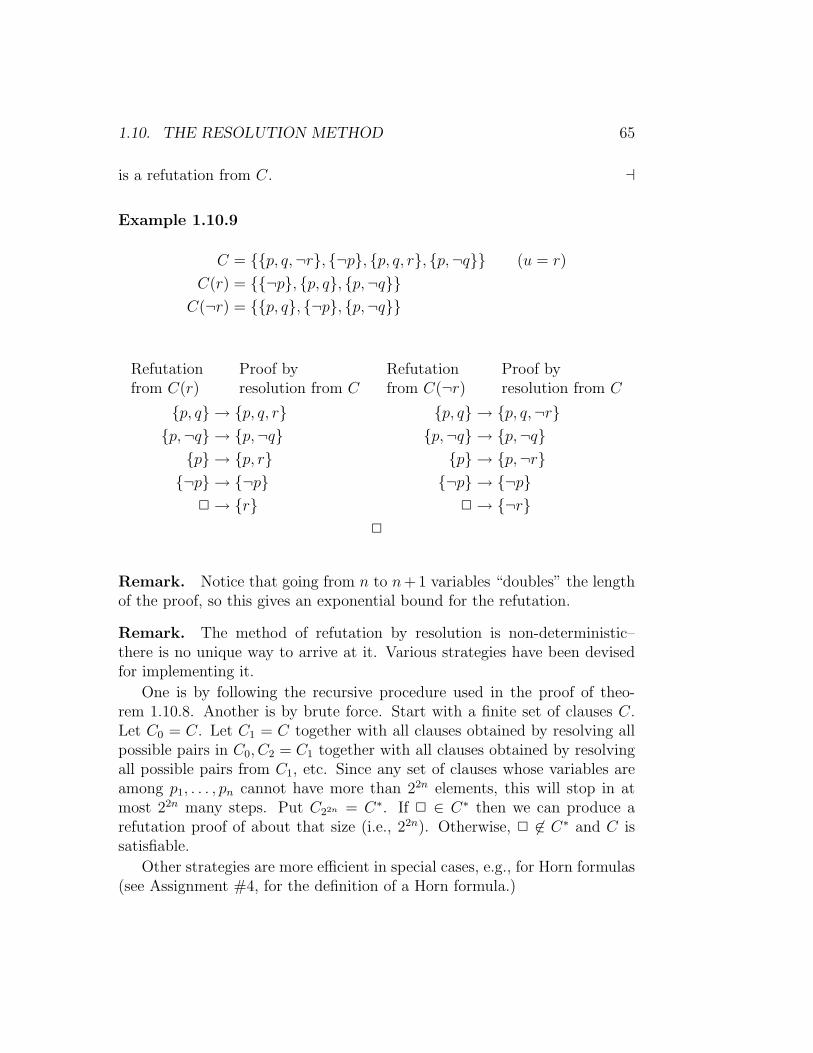
1.10. THE RESOLUTION METHOD 65
is a refutation from C. a
Example 1.10.9
C = {{p, q,¬r}, {¬p}, {p, q, r}, {p,¬q}} (u = r)
C(r) = {{¬p}, {p, q}, {p,¬q}}C(¬r) = {{p, q}, {¬p}, {p,¬q}}
Refutationfrom C(r)
Proof byresolution from C
Refutationfrom C(¬r)
Proof byresolution from C
{p, q} → {p, q, r} {p, q} → {p, q,¬r}{p,¬q} → {p,¬q} {p,¬q} → {p,¬q}
{p} → {p, r} {p} → {p,¬r}{¬p} → {¬p} {¬p} → {¬p}
2 → {r} 2 → {¬r}2
Remark. Notice that going from n to n+1 variables “doubles” the lengthof the proof, so this gives an exponential bound for the refutation.
Remark. The method of refutation by resolution is non-deterministic–there is no unique way to arrive at it. Various strategies have been devisedfor implementing it.
One is by following the recursive procedure used in the proof of theo-rem 1.10.8. Another is by brute force. Start with a finite set of clauses C.Let C0 = C. Let C1 = C together with all clauses obtained by resolving allpossible pairs in C0, C2 = C1 together with all clauses obtained by resolvingall possible pairs from C1, etc. Since any set of clauses whose variables areamong p1, . . . , pn cannot have more than 22n elements, this will stop in atmost 22n many steps. Put C22n = C∗. If 2 ∈ C∗ then we can produce arefutation proof of about that size (i.e., 22n). Otherwise, 2 6∈ C∗ and C issatisfiable.
Other strategies are more efficient in special cases, e.g., for Horn formulas(see Assignment #4, for the definition of a Horn formula.)

66 CHAPTER 1. PROPOSITIONAL LOGIC
1.11 A Hilbert-Type Proof System
We will now describe a different formal calculus of proofs, which correspondsmore directly to our intuitive concept of a “proof.” That is, it will startwith axioms and use rules of inference to deduce consequences, rather thandealing with abstract clause sets.
This style of arguing in formal logic, using axioms and rules, was intro-duced by David Hilbert and his school. Hilbert was born in Konigsberg,Prussia, in 1862, and died in Gottingen, Germany, in 1943. He is one of themost important mathematicians of the late 19-th and early 20-th century.A strong advocate of nonconstructive methods, this probably started withhis work on “invariant theory,” where he proved a Basis Theorem withoutexhibiting an explicit basis. The paper appeared in Mathematische Annalenin 1888. The result states that in any number of variables there is a finite setof generators for the invariants of quantics. A quantic is a symmetric tensorof a given degree constructed from tensor powers of a (finite dimensional)vector space. Invariance is measured under invertible operators of the spacein itself.
Gordon, the world expert in invariant theory, strongly opposed in vain tothe publication of Hilbert’s result, due to its nonconstructive nature. On theother hand, Klein said of this result that “I do not doubt this is the mostimportant work on general algebra that the Annalen has ever published.”
Hilbert’s work in number theory led to his book on the theory of algebraicnumber fields, recently translated into English. He started his work on logicwith the publication in 1899 of the Grundlagen der Geometrie, where headvocates the axiomatic approach to mathematics.
In 1900 he delivered the invited address “Mathematical problems” to theSecond International Congress of Mathematicians in Paris, where he listed 23problems that in his opinion were essential for the progress of mathematics.From here comes his dictum “Here is the problem, seek the solution”. Theinscription on his tombstone, “We must know, we will know” comes from aspeech in Konigsberg in 1938. His address can be found in the Bulletin ofthe AMS, vol 37, number 4 (2000).
His work on integral equations and calculus of variations led to functionalanalysis and the concept of Hilbert space. He also solved Waring’s problem,a well-known problem in number theory. His work in logic resulted in thedevelopment of proof systems and lead to the incompleteness theorems of K.Godel.

1.11. A HILBERT-TYPE PROOF SYSTEM 67
1.11.A Formal Proofs
It will be convenient here to consider as the basic symbols in the language ofpropositional logic the following:
¬,⇒, ), (, p1, p2, p3, . . .
and view (A ∧B), (A ∨B), (A ⇔ B) as abbreviations:
(A ∧B) : ¬(A ⇒ ¬B)
(A ∨B) : (¬A ⇒ B)
(A ⇔ B) : ¬((A ⇒ B) ⇒ ¬(B ⇒ A)).
A (logical) axiom is any formula of one of the following forms:
(i) A ⇒ (B ⇒ A)
(ii) (A ⇒ (B ⇒ C)) ⇒ ((A ⇒ B) ⇒ (A ⇒ C))
(iii) ((¬B ⇒ ¬A) ⇒ ((¬B ⇒ A) ⇒ B))
(for arbitrary A,B,C). Notice that each one of these is a tautology.We also have a rule of inference called modus ponens or MP: “From A
and A ⇒ B, derive B.” In formal calculi, a rule such as this for deriving oneformula from others given, is sometimes written as follows:
A, A ⇒ BB
.
Modus ponens is short for latin “modus ponendo ponens” which means“proposing method”. We can also draw this rule as a proof tree:
A A ⇒ B
B
Notice that A,A ⇒ B logically imply B.
Definition 1.11.1 Let S be any set (finite or infinite) of formulas. A formalproof from S is a finite sequence A1, A2, . . . , An of formulas such that eachAi is either a logical axiom, belongs to S or comes by applying modus ponensto some Aj, Ak with j, k < i (i.e., Ak is the formula Aj ⇒ An). We call thissequence a formal proof of An from S.

68 CHAPTER 1. PROPOSITIONAL LOGIC
Definition 1.11.2 If there is a formal proof of a formula A from S we saythat A is a formal theorem of S and write
S ` A.
If S = ∅, we just write` A
and call A a formal theorem.
Notice that S ` A and S ⊆ S ′ imply that S ′ ` A. Also notice that ifS ′ ` A and S ` B for all B ∈ S ′, then S ` A, since the formal proofs cansimply be concatenated. Finally, S ` A implies that there is finite S0 ⊆ Swith S0 ` A, since a formal proof can only be finitely long and hence canonly use finitely many formulas of S.
Example 1.11.3 S = {(A ⇒ B), A ⇒ (B ⇒ C), A}. Here is a formalproof of C from S:
1. A ⇒ (B ⇒ C) (in S)2. ((A ⇒ (B ⇒ C)) ⇒ ((A ⇒ B) ⇒ (A ⇒ C))) (axiom (ii))3. (A ⇒ B) ⇒ (A ⇒ C) (MP from 1, 2)4. A ⇒ B (in S)5. A ⇒ C (MP from 3, 4)6. A (in S)7. C (MP from 5, 6)
We can also write this as a proof tree:
A
A ⇒ B
A ⇒ (B ⇒ C) (A ⇒ (B ⇒ C)) ⇒ ((A ⇒ B) ⇒ (A ⇒ C))
(A ⇒ B) ⇒ (A ⇒ C)
A ⇒ C
C
Example 1.11.4 The following formal proof shows that ` A ⇒ A:

1.11. A HILBERT-TYPE PROOF SYSTEM 69
1. (A ⇒ ((A ⇒ A)︸ ︷︷ ︸B
⇒ A︸︷︷︸C
)) ⇒ ((A ⇒ (A ⇒ A)︸ ︷︷ ︸B
) ⇒ (A ⇒ A︸︷︷︸C
))
(Ax. (ii))2. A ⇒ ((A ⇒ A)︸ ︷︷ ︸
B
⇒ A) (Ax. (i))
3. ((A ⇒ (A ⇒ A)) ⇒ (A ⇒ A)) (MP 1, 2)4. A ⇒ (A ⇒ A) (Ax. (i))5. A ⇒ A (MP 3, 4).
The main result about this formal proof system is the following:
Theorem 1.11.5 For any set of formulas S, and any formula A:
S |= A iff S ` A.
One direction of this theorem, i.e. the soundedness of the proof system(S ` A implies that S |= A) is easy, and we prove it first.
1.11.B Soundness
Given a property P (A) of formulas, suppose we want to prove that P (A)holds for all formal theorems of S, i.e., we want to show that if S ` A, thenP (A) holds. We can do this by the following form of induction:
Basis.
(i) Show that P (A) holds, when A is a logical axiom;
(ii) Show that P (A) holds when A is in S.
Induction Step. Assuming that P (A), P (A ⇒ B) hold, and show thatP (B) holds.
We call this induction on proofs of A from S.In our case P (A) is the property
“S |= A”.
The basis of the induction is clear: S |= A is certainly correct if A is in S orelse A is a logical axiom (since it is then a tautology). The induction step isequally simple: If S |= A and S |= A ⇒ B, clearly S |= B.

70 CHAPTER 1. PROPOSITIONAL LOGIC
1.11.C Completeness
To prove the hard direction of the theorem, i.e. the completeness of theproof system, it will be convenient to develop first some basic propertiesof this system. These are useful independently of this and can help, forexample, in constructing formal proofs. They are indeed formal analogs ofsome commonly used proof techniques. They are theorems about formalproofs and theorems, and so often called metatheorems.
Proposition 1.11.6 (The Deduction Theorem) If S ∪ {A} ` B, thenS ` A ⇒ B.
Remark. It is easy to see that if S ` A ⇒ B, then S ∪ {A} ` B.
Proof. We will show this by induction on proofs of B from S ∪ {A}.Basis.
(i) B is a logical axiom. Then clearly S ` B. But B ⇒ (A ⇒ B)is a logical axiom, thus S ` B ⇒ (A ⇒ B), so, by modus ponens,S ` A ⇒ B.
(ii) B is in S ∪ {A}. There are two subcases:
(a) B is in S. Then again S ` B and the proof is completed as in (i).
(b) B = A. Then ` A ⇒ A by example 1.11.4, so S ` A ⇒ A, whichis the same as S ` A ⇒ B
Induction step. We assume that we have shown that S ` A ⇒ (B ⇒ C)and S ` A ⇒ B, and want to show that S ` A ⇒ C. Now ((A ⇒ (B ⇒C)) ⇒ ((A ⇒ B) ⇒ (A ⇒ C)) is a logical axiom, so
S ` ((A ⇒ (B ⇒ C)) ⇒ ((A ⇒ B) ⇒ (A ⇒ C)),
and then, by MP applied twice, we have
S ` A ⇒ C.
a

1.11. A HILBERT-TYPE PROOF SYSTEM 71
Definition 1.11.7 We call a set of formulas S formally inconsistent if forsome formula A,
S ` A and S ` ¬A.
Otherwise, S is formally consistent.
Proposition 1.11.8 (Proof by Contradiction) If S∪{A} is formally in-consistent, then S ` ¬A.
Proof. Left for Assignment #5. aProposition 1.11.9 (Proof by Contrapositive) If S ∪ {A} ` ¬B, thenS ∪ {B} ` ¬A.
Proof. Left for Assignment #5. aWe embark now on the proof of the Completeness of our proof system.
We claim that it is enough to show the following:
If a set of formulas S is formally consistent, then it is satisfiable. (∗)To see this, assume (∗) has been proved. If S |= A, then S ∪ {¬A} isunsatisfiable, so by (∗), applied to S∪{¬A}, S∪{¬A} is formally inconsistent.Thus, by proof by contradiction, S ` ¬¬A, so by Assignment #5, Problem1, S ` A, which is what we wanted. So it remains to prove (∗).
The idea of the proof is as follows: Let us call a set of formulas S completeif for any formula A,
A ∈ S or ¬A ∈ S.
We will first prove that if S is a given formally consistent set of formulas,then we can find a formally consistent set of formulas S ⊇ S which is alsocomplete. Then for any propositional variable pi we must have that exactlyone of the following holds
pi ∈ S or ¬pi ∈ S.
Thus we can define a valuation ν by letting
ν(pi) =
{1 if pi ∈ S
0 if ¬pi ∈ S.
It will then turn out that ν is a valuation that satisfies S and so S, i.e., S issatisfiable. Let’s implement this plan.

72 CHAPTER 1. PROPOSITIONAL LOGIC
Lemma 1.11.10 Let S be a formally consistent set of formulas. Then wecan find a formally consistent and complete set of formulas S such that S ⊆S.
Proof. First we can enumerate in a sequence A1, A2, . . . all formulas. Thenwe can define recursively a sequence
S0 = S, S1, S2, . . .
of formulas such that
S0 ⊆ S1 ⊆ S2 ⊆ . . .
as follows:
S0 = S,
Sn+1 =
{Sn ∪ {An+1} if S ∪ {An+1} is formally consistent
Sn ∪ {¬An+1} otherwise.
We claim then that each Sn is formally consistent. We do this easily byinduction using the following sublemma.
Sublemma 1.11.11 If T is a formally consistent set of formulas and Ais any formula, then at least one of T ∪ {A}, T ∪ {¬A} is still formallyconsistent.
Proof. Otherwise both T ∪ {A}, T ∪ {¬A} are formally inconsistent. SoT ` A by proof of contradiction and Assignment #5, Problem 1, and sinceclearly T ` B for any B ∈ T , it follows that T ` B for any B ∈ T∪{A}. SinceT ∪ {A} is formally inconsistent, this shows that T is formally inconsistent,a contradiction. a
Now let S =⋃∞
n=1 Sn. We claim this works. First S is complete, sinceif A is any given formula, then A = An for some n and so by constructioneither A ∈ Sn or ¬A ∈ Sn, i.e., A ∈ S or ¬A ∈ S. Finally S is stillformally consistent, since otherwise S ` A, S ` ¬A for some formula A.Then by definition of a formal proof, there is a finite subset S∗ ⊆ S suchthat S∗ ` A, S∗ ` ¬A. But then for some large enough n we have S∗ ⊆ Sn,so Sn ` A, Sn ` ¬A, and so Sn is formally inconsistent, a contradiction. a
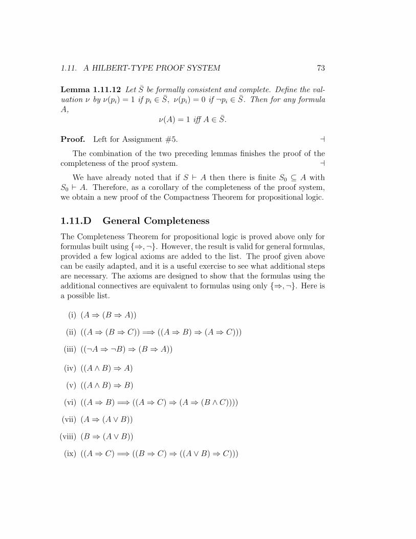
1.11. A HILBERT-TYPE PROOF SYSTEM 73
Lemma 1.11.12 Let S be formally consistent and complete. Define the val-uation ν by ν(pi) = 1 if pi ∈ S, ν(pi) = 0 if ¬pi ∈ S. Then for any formulaA,
ν(A) = 1 iff A ∈ S.
Proof. Left for Assignment #5. aThe combination of the two preceding lemmas finishes the proof of the
completeness of the proof system. aWe have already noted that if S ` A then there is finite S0 ⊆ A with
S0 ` A. Therefore, as a corollary of the completeness of the proof system,we obtain a new proof of the Compactness Theorem for propositional logic.
1.11.D General Completeness
The Completeness Theorem for propositional logic is proved above only forformulas built using {⇒,¬}. However, the result is valid for general formulas,provided a few logical axioms are added to the list. The proof given abovecan be easily adapted, and it is a useful exercise to see what additional stepsare necessary. The axioms are designed to show that the formulas using theadditional connectives are equivalent to formulas using only {⇒,¬}. Here isa possible list.
(i) (A ⇒ (B ⇒ A))
(ii) ((A ⇒ (B ⇒ C)) =⇒ ((A ⇒ B) ⇒ (A ⇒ C)))
(iii) ((¬A ⇒ ¬B) ⇒ (B ⇒ A))
(iv) ((A ∧B) ⇒ A)
(v) ((A ∧B) ⇒ B)
(vi) ((A ⇒ B) =⇒ ((A ⇒ C) ⇒ (A ⇒ (B ∧ C))))
(vii) (A ⇒ (A ∨B))
(viii) (B ⇒ (A ∨B))
(ix) ((A ⇒ C) =⇒ ((B ⇒ C) ⇒ ((A ∨B) ⇒ C)))

74 CHAPTER 1. PROPOSITIONAL LOGIC
(x) ((A ⇔ B) ⇒ (A ⇒ B))
(xi) ((A ⇔ B) ⇒ (B ⇒ A))
(xii) ((A ⇒ (B ⇒ C)) =⇒ ((A ⇒ (C ⇒ B)) ⇒ (A ⇒ (B ⇔ C))))

Chapter 2
First-Order Logic
2.1 Structures
2.1.A Relations and Functions
Definition 2.1.1 Let A be a nonempty set and let n = 1, 2, . . . . An n-aryrelation or predicate on A is a subset R ⊆ An, where An = {(a1, . . . , an) :a1, . . . , an ∈ A} is the set of ordered n-tuples of elements of A. We call n thearity of R.
Examples 2.1.2(i) A = N (= {0, 1, 2, . . . })
R = {n ∈ N : n is even} ⊆ N (unary (1-ary))
S = {(m,n) ∈ N2 : m < n} ⊆ N2 (binary (2-ary))
T = {(m,n, p) ∈ N3 : m ≡ n mod (p)} ⊆ N3 (ternary (3-ary))
(ii) A = R (= the set of reals)
Q = {x ∈ R : x is rational} ⊆ R (unary)
P = {(x, y) ∈ R2 : y = x2} ⊆ R2 (binary)
U =
(a1, . . . , an) ∈ Rn :a1x
n−1 + a2xn−2 + · · ·+ an−1x + an
has n− 1 real solutions.
(n-ary)
B = {(x, y, z) : y is between x and z} (ternary)
75

76 CHAPTER 2. FIRST-ORDER LOGIC
(iii) A = V , where G = 〈V, E〉 is a graph with set of vertices V and set ofedges E.
E = {(x, y) ∈ V 2 : x and y are connected by an edge} (binary)
F =
{(x, y) ∈ V 2 :
x and y are connected by a pathx0 = x, x1, . . . , xn−1, xn = y.
}(binary)
Remark. If R ⊆ An is an n-ary relation, we also view R as expressing aproperty of n-tuples (a1, . . . , an) ∈ An and we often write
R(a1, . . . , an),
instead of
(a1, . . . , an) ∈ R.
Thus R(a1, . . . , an) means that (a1, . . . , an) has property R or satisfies R.Note that a 1-ary relation is a property of single elements of A, or alternatelyjust the subset of A containing all elements with that property.
Example 2.1.3 For R, S, T as in examples 2.1.2 (i) above:
(i) R(n) means “n is even”
(ii) S(m,n) means “m < n”
(iii) T (m,n, p) means “m ≡ n mod (p)
Remark. Example 2.1.3 (ii) above says that S essentially is the familiar“less than” relation, so we can write “< (a, b)” or even just “a < b” insteadof S(a, b). The same holds true for other familiar binary relations.
Definition 2.1.4 Let again A be any nonempty set. A n-ary function oroperation on A is a map
f : An → A,
in other words, a rule for assigning to each element (x1, . . . , xn) of An (whereeach xi ∈ A) an element f(x1, . . . , xn) of A, called the value of the functionat (x1, . . . , xn). We call n the arity of f .
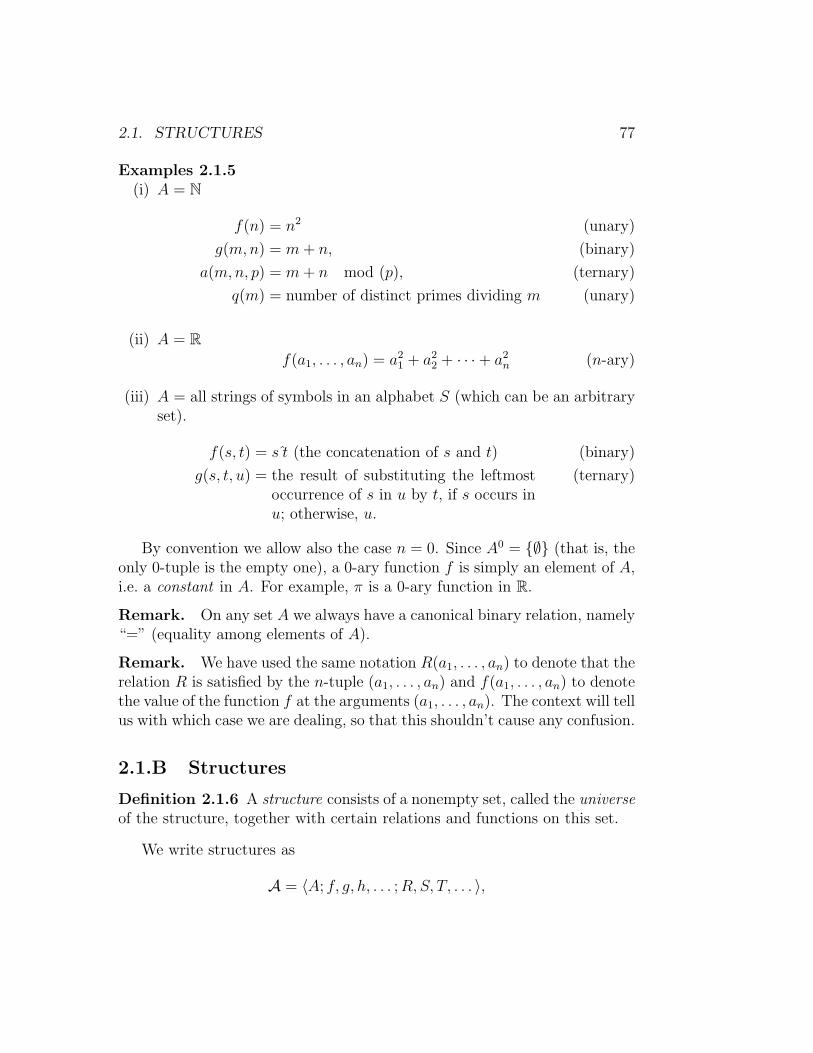
2.1. STRUCTURES 77
Examples 2.1.5(i) A = N
f(n) = n2 (unary)
g(m,n) = m + n, (binary)
a(m,n, p) = m + n mod (p), (ternary)
q(m) = number of distinct primes dividing m (unary)
(ii) A = Rf(a1, . . . , an) = a2
1 + a22 + · · ·+ a2
n (n-ary)
(iii) A = all strings of symbols in an alphabet S (which can be an arbitraryset).
f(s, t) = s t (the concatenation of s and t) (binary)
g(s, t, u) = the result of substituting the leftmostoccurrence of s in u by t, if s occurs inu; otherwise, u.
(ternary)
By convention we allow also the case n = 0. Since A0 = {∅} (that is, theonly 0-tuple is the empty one), a 0-ary function f is simply an element of A,i.e. a constant in A. For example, π is a 0-ary function in R.
Remark. On any set A we always have a canonical binary relation, namely“=” (equality among elements of A).
Remark. We have used the same notation R(a1, . . . , an) to denote that therelation R is satisfied by the n-tuple (a1, . . . , an) and f(a1, . . . , an) to denotethe value of the function f at the arguments (a1, . . . , an). The context will tellus with which case we are dealing, so that this shouldn’t cause any confusion.
2.1.B Structures
Definition 2.1.6 A structure consists of a nonempty set, called the universeof the structure, together with certain relations and functions on this set.
We write structures as
A = 〈A; f, g, h, . . . ; R, S, T, . . . 〉,

78 CHAPTER 2. FIRST-ORDER LOGIC
where A is the universe, f, g, h, . . . are the functions of the structure, andR, S, T, . . . are the relations of the structure. Note that A can be finite orinfinite (but not empty), and there can be any number (finite, infinite, oreven zero) of functions, each with any arity n ≥ 0, and any number (finite,infinite, or zero) of relations, each with any arity n ≥ 1.
A structure codifies a context, of mathematical or other objects, whichwe study. The universe of the structure encompasses all the objects underconsideration and the functions and relations of the structure are the basicor primitive operations and relations between these objects that we want tostudy.
Definition 2.1.7 The signature of A is
〈arity(f), arity(g), arity(h), . . . ; arity(R), arity(S), arity(T ), . . . 〉.Examples 2.1.8
(i) The structure of (natural number) arithmetic:
N = 〈N; 0, S, +, ·; <〉.It has signature
〈0, 1, 2, 2; 2〉.(Here S(n) = n + 1 is the “successor” function.)
(ii) The structure of the reals :
R = 〈R; 0, 1, +, ·; 〉.It has signature
〈0, 0, 2, 2; 〉.This structure represents the basic algebra of real numbers. If we wantto study something different, such as elementary trigonometry, a moreappropriate structure might be 〈R; 0, 1, +, ·, sin, cos, . . . 〉.
(iii) Let X be an arbitrary set (finite or infinite). Then
〈P (X); ∅,∩,∪;⊆〉,where P (X) is the collection of all subsets of X, is a structure withsignature
〈0, 2, 2; 2〉.

2.1. STRUCTURES 79
(iv) Many algebraic structures are simply structures in the above sense,which satisfy certain properties (axioms). For example, a group is astructure of the form
〈G; e, ·; 〉of signature 〈0, 2; 〉 satisfying the group laws.
(v) A graph is a structure of the form
〈V ; ; E〉
of signature 〈; 2〉 satisfying the usual conditions.
(vi) Let S be the set of records of employees in some company (contain-ing, e.g., social security numbers, dates of birth, salary, etc.), let N ={0, 1, . . . , n} for n a large enough integer, and let
A = 〈S ∪N ; f, g, h; P, Q,R〉,
where
f(x) =
{the age of the employee with record x if x ∈ S
0 otherwise.
g(x) =
{the SSN of the employee with record x if x ∈ S
0 otherwise.
h(x) =
{the salary of the employee with record x if x ∈ S
0 otherwise.
P (x) iff x ∈ S
Q(x) iff x ∈ N
R(x, y) iff x is a supervisor of y.
Then A is a structure of arity 〈1, 1, 1; 1, 1, 2〉. This example shows howwe can include both the objects we want to study (here, the records)and some basic mathematical tools to use in reasoning about them(here, some natural numbers) in a single structure.

80 CHAPTER 2. FIRST-ORDER LOGIC
2.1.C Introduction to First-Order Languages
We now want to describe a formal language in which we can express state-ments about structures. We will give a series of examples showing how todevelop such a language.
Example 2.1.9 Consider the statement:
“The square of an odd number is odd.”
This is a statement about the structure of arithmetic,
N = 〈N; 0, S, +, ·; <〉.We now introduce the following notation:
x, y, z, . . . variables representing arbitrary natural numbers;¬,∧,∨,⇒,⇔ the usual propositional connectives;(, ) parentheses;∃ (there exists), the existential and∀ (for all) universal quantifier;= symbol for equality;0, S, +, ·, < symbols for the operations and relations of N .
In order to write this statement in a formal language using these symbols,we must first express it in a more precise form:
“For all natural numbers x, if x is odd, then x · x is odd.”
We must further refine this by replacing “x is odd” with
“There exists a natural number y such that x = 2 · y + 1.”
Finally, since 1 and 2 are not constants in the structure of arithmetic, wemust replace them with S(0) and S(S(0)), respectively. We can now expressthe above statement in a formal language as:
∀x[∃y(x = S(S(0)) · y + S(0)) ⇒ ∃z(x · x = S(S(0)) · z + S(0))]
We often use abbreviations, however, such as
S(0) = 1, S(S(0)) = 2, x · x = x2, u · v = uv,
Using these abbreviations, our statement becomes more readable:
∀x[∃y(x = 2y + 1) ⇒ ∃z(x2 = 2z + 1)].

2.2. SYNTAX OF FIRST-ORDER LOGIC 81
Example 2.1.10 “Every non-empty subset of N has a least element”.The appropriate structure here is:
〈N ∪ P (N); N, S,∈, <〉,
whereP (N) = {A : A ⊆ N} = the power set of N
N(a) iff a ∈ NS(a) iff a ∈ P (N) (i.e., a ⊆ N)
a ∈ b iff a ∈ N, b ∈ P (N), and a is an element of b
a < b iff a, b ∈ N and a is smaller than b
Using the same logical notation as before and symbols N, S,∈, < for therelations of this structure we can express the previous statement as
∀x[(S(x) ∧ ∃y(y ∈ x)) ⇒ ∃z(z ∈ x ∧ ∀w(w ∈ x ⇒ z = w ∨ z < w))]
2.2 Syntax of First-Order Logic
We will now give a formal definition of the languages which were discussedby example in section 2.1.C.
2.2.A Symbols
Definition 2.2.1 A first-order language has the following set of symbols(alphabet):
(i) Logical symbols :
x1, x2, x3, . . . (variables)¬,∧,∨,⇒,⇔ (propositional connectives)∃, ∀ (quantifiers)(, ) (parentheses)= (equality symbol)
(ii) Non-logical symbols :

82 CHAPTER 2. FIRST-ORDER LOGIC
(a) For each n ≥ 0 a set Fn (which may be empty) of symbols called n-ary function symbols (or function symbols of arity n). For n = 0,the symbols in F0 are called constant symbols.
(b) For each n ≥ 1, a set Rn (which may be empty) of symbols calledn-ary relation symbols (or relation symbols of arity n).
Remark. All these sets of symbols are of course assumed to be pairwisedisjoint. The equality symbol = is also a binary relation symbol, but playsa special role.
Remark. A first-order language is completely determined by its set L =⋃nFn ∪
⋃nRn of non-logical symbols (since the set of logical symbols is the
same for all first-order languages).
Examples 2.2.2(i) An example of a first-order language is L = {c, f, g; R}, where c is
a constant symbol, f a unary function symbol, g a binary functionsymbol, and R a binary relation symbol.
(ii) A more meaningful example is the language of arithmetic:
Lar = {0, S, +, ·; <}where 0 is a constant symbol, S a unary function symbol, + and ·binary function symbols, and < a binary relation symbol. This is thelanguage that was used in example 2.1.9.
2.2.B Terms
We will now start defining the “grammatically correct” statements of a first-order language. We begin by defining strings called terms. Each term isintended to represent a single element of the structure. Terms are definedrecursively as follows.
Definition 2.2.3 (Terms)(i) Every variable symbol is a term.
(ii) If t1, . . . , tn are terms and f is an n-ary function symbol, then ft1 . . . tnis a term. Note that if n = 0, i.e. f is a constant symbol, then f is aterm all by itself.

2.2. SYNTAX OF FIRST-ORDER LOGIC 83
Thus we use “Polish notation” to represent terms. (The weight of eachn-ary function symbol is 1− n and that of constant symbols and variables is1.)
Example 2.2.4 Suppose L contains the constant symbols a, b, the unaryfunction symbol g and the binary function symbols f, h. Then the followingis a term in this language
fgahbx1.
This can be also represented by a parse tree as follows:
a
gga
b x1
hbx1
h
fgahbx1
f
As in section 1.2.C, we have unique readability, in the sense that everyterm can be uniquely written as: xi, a (constant symbol) or ft1 . . . tn, foruniquely determined t1, . . . , tn terms and f an n-ary function symbol (n ≥ 1).
To facilitate reading, we will add parentheses and adopt the followinginformal notation:
f(t1, . . . , tn) instead of ft1 . . . tn
So we would write the term in the example above as
f(g(a), h(b, x1)).
Also, for familiar binary function symbols f (like +, ·, etc) we will usuallywrite
(tfs) instead of fts,
and when there is no confusion we will even drop the parentheses and writetfs.
Finally, we often use x, y, z, . . . for variables instead of x1, x2, . . . .
Example 2.2.5 In the language of arithmetic, the following are terms (usingour informal notation, that is):

84 CHAPTER 2. FIRST-ORDER LOGIC
(x + y) · z (instead of ·+ xyz)(x · x) + (y · y)((x · x) · x + S(0) · x) + S(S(0))
In fact, all terms in this language are polynomials in several variables withcoefficients in N. We can view terms in arbitrary languages as “generalizedpolynomials.”
Notation. If the variables occurring in a term t are among x1, . . . , xn, weindicate this by writing t(x1, . . . , xn). Note that this does not mean that allof x1, . . . , xn occur in t. If u1, . . . , un are terms, then
t[x1/u1, . . . , xn/un]
denotes the result of substituting each variable xi in t by ui. By inductionon the construction of t, this is also a term.
Example 2.2.6 If
t(x, y) is f(g(x), h(a, y)),
then
t[x/g(a), y/h(a, x))] is f(g(g(a)), h(a, h(a, x)).
2.2.C Well-Formed Formulas
We can now define the statements in first-order languages, which we again call(well-formed) formulas (wffs). We start with the simplest possible formulas.
Definition 2.2.7 An atomic formula is any string of the form
Rt1 . . . tn
with R an n-ary relation symbol and t1, . . . , tn terms.
Example 2.2.8 Let L = {a, b, f, g, R}, a, b constant symbols, f a unaryfunction symbol, g a binary function symbol, R a ternary relation symbol.The following are atomic formulas in this language:
Rfagxay, = gxyfa

2.2. SYNTAX OF FIRST-ORDER LOGIC 85
Example 2.2.9 Let L = {<}, < a binary relation symbol. Then the fol-lowing is an atomic formula:
< xy.
Again we have unique readability: every atomic formula is of the formRt1 . . . tn for uniquely determined R, t1, . . . , tn.
And as we did with terms, we adopt various convenient informal nota-tions. We write
R(t1, . . . , tn) instead of Rt1 . . . tn.
For familiar binary relation symbols R (like =, <), we write
(tRs) instead of Rts,
and when there is no chance of confusion we often omit the parentheses aswell, writing tRs. So in example 2.2.8 we would write R(f(a), g(x, a), y) and(g(x, y) = f(a)), and in example 2.2.9 we would write (x < y) or even x < y.
Finally, we are ready to define:
Definition 2.2.10 (Well-Formed Formulas)(i) Every atomic formula is a wff.
(ii) If A,B are wff, so are ¬A, (A ∧B), (A ∨B), (A ⇒ B), (A ⇔ B).
(iii) If A is a wff and xi a variable, then ∃xiA, ∀xiA are wff.
Examples 2.2.11(i) Let L = {<}, < a binary relation symbol. Then
∀x∃y(x < y)
is a wff, as is justified by the following parsing sequence:
(x < y), ∃y(x < y), ∀x∃y(x < y).
(ii) In the same language,
∀x∀y∀z((x < y) ∧ (y < z) ⇒ (x < z))
is a wff, as justified by the following parsing sequence:
(x < y), (y < z), (x < z), (x < y) ∧ (y < z),

86 CHAPTER 2. FIRST-ORDER LOGIC
((x < y) ∧ (y < z) ⇒ (x < z))︸ ︷︷ ︸A
, ∀zA, ∀y∀zA, ∀x∀y∀zA.
We can also represent any wff by a parse tree. For (ii) this would be
(x < y) (y < z)
(x < y) ∧ (y < z)
∧x < z
A⇒
∀z∀zA∀y
∀y∀zA∀x
∀x∀y∀zA
(iii) L = {R,Q, S}, with R ternary and Q,S unary relation symbols. Thefollowing is a formula:
∃x(∀yR(x, y, z) ⇒ (¬Q(x) ∨R(y))).
Yet again we have unique readability: every formula is in exactly one ofthe forms:
(i) atomic;
(ii) ¬A, (A ∧ B), (A ∨ B), (A ⇒ B), (A ⇔ B) for uniquely determinedA,B;
(iii) ∃xiA, ∀xiA for uniquely determined xi, A.
Definition 2.2.12 A subformula of a formula A is any formula occurring inthe parse tree of A.

2.2. SYNTAX OF FIRST-ORDER LOGIC 87
2.2.D Scope and Free Variables
Proposition 2.2.13 Let A be a wff, Q be either ∃ or ∀, x a variable. Forany occurrence of the string Qx in A we have A = SQxBT , where S, T arestrings and B is a uniquely determined wff called the scope of this occurrenceof Qx.
Example 2.2.14 P (x, y) ⇒ ∀x [∃y R(x, y)︸ ︷︷ ︸scope
⇒ ∀xQ(x, y)]︸ ︷︷ ︸scope︸ ︷︷ ︸
scope
Example 2.2.15 ∃y ∀x [∃y R(x, y)︸ ︷︷ ︸scope
⇒ Q(x, y)]
︸ ︷︷ ︸scope︸ ︷︷ ︸
scope
Proof of proposition 2.2.13. It is easy to prove by induction on theconstruction of A that for any occurrence of Qx in A we have A = SQxBTfor some wff B and some strings S, T . Uniqueness follows from the fact that aproper nonempty initial segment of a wff is not a wff (see Assignment #6).a
Definition 2.2.16 An occurrence of a variable x in a formula A is bound if itoccurs in a substring of the form QxB, where B is the scope of x. Otherwisethis occurrence is called free.
Example 2.2.17 In example 2.2.14 the first occurrences of x, y and the lastoccurrence of y are free. All the other occurrences are bound. In exam-ple 2.2.15, all occurrences are bound.
Definition 2.2.18 A variable x is free in a wff A if it has at least one freeoccurrence. It is bound if it has at least one bound occurence.
Note that a variable can be both free and bound. This is in contrast toa single occurrence of a variable, which is either one or the other.
Example 2.2.19 In example 2.2.14, x, y are both free and bound. In 2.2.15x, y are bound but not free. In R(x, y) they are free but not bound. In∃xR(x, y), x is bound and not free, and y is free but not bound.
88 CHAPTER 2. FIRST-ORDER LOGIC
Remark. This should be compared with a notation such as∫
(x2 + y)dx.Here x is “bound” and y is “free.”
Bound variables are sometimes called “dummy variables,” since they canbe replaced with a different variable (which does not appear elsewhere)without changing the meaning of the formula. That is,
∫(x2 + y)dx and∫
(t2 +y)dt are equivalent. And once we define equivalence of wffs, pairs suchas ∀x(x < y) and ∀z(z < y) will be equivalent as well: see fact 2.3.17.
Notation. A(x1, . . . , xn) means that the free variables of A are amongx1, . . . , xn. So in example 2.2.14, we would write A(x, y).
Definition 2.2.20 A sentence is a wff with no free variables.
Example 2.2.21 ∀x∃y(x < y) is a sentence, as is example 2.2.15, but 0 < xis not, nor is example 2.2.14.
2.3 Semantics of First-Order Logic
Now we will connect the first-order languages to the structures we intendedthem to represent.
2.3.A Structures and Interpretations
Definition 2.3.1 Let L =⋃
n≥0Fn ∪⋃
n≥1Rn be a first-order language. Astructure M for L consists of:
(i) a nonempty set M (the universe of this structure)
(ii) an n-ary function fM : Mn → M for each f ∈ Fn. (For n = 0, i.e.a ∈ F0 is a constant symbol, aM is simply an element of M .)
(iii) an m-ary relation RM ⊆ Mm for each R ∈ Rm.
We write this as
M = 〈M, {fM}f∈Sn≥0 Fn , {RM}R∈Sn≥1Rn〉,
and call fM the interpretation of f and RM the interpretation of R in M.

2.3. SEMANTICS OF FIRST-ORDER LOGIC 89
Example 2.3.2 If
L = {function symbols︷ ︸︸ ︷
a, f, g ;
relation symbols︷︸︸︷S, R }
(a is a constant; f unary; g binary; S binary, R ternary), then a structurefor L has the form
M = 〈M ; aM, fM, gM; SM, RM〉,with aM ∈ M, fM : M → M, gM : M2 → M, SM ⊆ M2, RM ⊆ M3.
Example 2.3.3 Let Lar = {0, S, +, ·, <} be the language of arithmetic.Then
N = 〈N ; 0, S, +, ·; <〉is a structure for Lar called the standard structure of this language. Anotherstructure for this language is
A = 〈A; 0A, SA, +A, ·A; <A〉,where A = R, 0A = π, SA(a) = ea,A+A b = a + b, a ·A b = a · b, a <A b iffb = cos(a).
Given a structure M = 〈M, . . . 〉 for L, we can assign to each termt(x1, . . . , xn) of L an n-ary function tM : Mn → M by recursion as follows:
(i) If t is a variable xi, then i ≤ n, and we let tM(a1, . . . , an) = ai.
(ii) If t is a constant c, then tM(a1, . . . , an) = cM.
(iii) If t = f(t1, . . . , tk), then
tM(a1, . . . , an) = fM(tM1 (a1, . . . , an), . . . , tMk (a1, . . . , an)).
Definition 2.3.4 We call tM(a1, . . . , an) the evaluation or interpretation oft at a1, . . . , an in M.
Remark. If t = t() has no variables, then tM is simply an element of M.
Remark. If t = t(x1, . . . , xn), then also t = t(x1, . . . , xn, xn+1, . . . , xk) forany k > n and strictly speaking we have an infinite list of functions tMn ,one for each n such that all the variables of t are among x1, . . . , xn. Noticehowever that for n < k, tMn (a1, . . . , an) = tMk (a1, . . . , an, an+1, . . . , ak).
90 CHAPTER 2. FIRST-ORDER LOGIC
Example 2.3.5 Let Lar = {0, S, +, ·, <} and N = 〈N; 0, S, +, ·; <〉 its stan-dard structure. Then if
t(x, y) = (x · x + y) + S(S(0)),
we have
tN : N2 → N,
tN (a, b) = a2 + b + 2.
2.3.B Models and Validities
Now let L be a first-order language, A a wff in L, M a structure for L, andconsider an assignment xi 7→ ai which associates with each variable xi anelement ai of M (the universe of M).
Definition 2.3.6 We say that A is true in M under this assignment, whichwe write
M, a1, a2, . . . |= A,
if the following recursive definition is satisfied:
(i) If A is atomic, say A = R(t1, . . . , tk), with ti = ti(x1, . . . , xn), then
M, a1, a2, . . . |= A iff RM(tM1 (a1, . . . , an), . . . , tMk (a1, . . . , an)).
Here we understand that if R is the equality symbol =, then =M is theequality on M , so
M, a1, a2, . . . |= t1 = t2 iff tM1 (a1, . . . , an) = tM2 (a1, . . . , an).
(ii) M, a1, a2, . . . |= ¬A iff it is not the case that M, a1, a2, . . . |= A (i.e.M, a1, a2, · · · 6|= A)
M, a1, a2 . . . |= A ∧B iff M, a1, a2, . . . |= A and M, a1, a2, . . . |= B
M, a1, a2 . . . |= A ∨B iff M, a1, a2, . . . |= A or M, a1, a2, . . . |= B
M, a1, a2 . . . |= A ⇒ B iff M, a1, a2, · · · 6|= A or M, a1, a2, . . . |= B
M, a1, a2 . . . |= A ⇔ B iff either M, a1, a2 . . . |= A,B orM, a1, a2 · · · 6|= A,B

2.3. SEMANTICS OF FIRST-ORDER LOGIC 91
(iii) M, a1, a2, . . . , ai, . . . |= ∃xiA iff for some bi ∈ M ,
M, a1, a2, . . . , ai−1, bi, ai+1, . . . |= A;
M, a1, a2, . . . , ai, . . . |= ∀xiA iff for all bi ∈ M ,
M, a1, a2, . . . , ai−1, bi, ai+1, . . . |= A.
It is easy to show by induction on the construction of A, that if
A(x1, . . . , xn)
is given and ai, bi (i = 1, 2, . . . ) ∈ M are such that ai = bi for all i ≤ n, then
M, a1, a2, . . . |= A iff M, b1, b2, . . . |= A,
so we abbreviateM, a1, a2, . . . |= A
byM |= A[a1, . . . , an]
or if we need to be more explicit
M |= A[x1 7→ a1, x2 7→ a2, . . . , xn 7→ an].
We read this as: Mmakes A[a1, . . . , an] true or A is satisfied inM, a1, . . . , an.
Definition 2.3.7 In particular, if A = A() is a sentence (has no free vari-ables), we simply write
M |= A,
and say that M satisfies A or A is true in M. We also say that M is amodel of A.
Example 2.3.8 Let L = {<} (< a binary relation symbol) andM = 〈N, <〉,and consider the following wffs:
(i) A : x < y. Then we have
M |= x < y[2, 3] (i.e. 2 < 3)
M |= ¬x < y[2, 1] (i.e. 2 6< 1).

92 CHAPTER 2. FIRST-ORDER LOGIC
(ii) B : ∃x∀y(x < y ∨ x = y), a sentence. Then
M |= ∃x∀y(x < y ∨ x = y). (2.1)
By definition this means that there is a ∈ N so that M |= ∀y(x <y ∨ x = y)[x 7→ a], and again, by definition, this means that for allb ∈ N,
M |= (x < y ∨ x = y)[x 7→ a, y 7→ b].
so equation (2.1) means that for some a ∈ N, and all b ∈ N, a < b ora = b, i.e. a ≤ b. Clearly a = 0 works.
If on the other hand we take S = 〈Z, <〉, a different model for L, then
S |= ¬∃x∀y(x < y ∨ x = y).
Example 2.3.9 Let Lar = {0, S, +, ·, <} be the language of arithmetic andN = 〈N, 0, S, +, ·, <} its standard structure. Then the following are true:
N |= ∀x∀y(x + S(y) = S(x + y))
N |= ∀x∃y1∃y2∃y3∃y4(x = y1 · y1 + y2 · y2 + y2 · y3 + y4 · y4)
(parentheses omitted by association to the left.) The latter is because everynatural number is the sum of four squares—Lagrange’s Theorem.
N |= ¬∀x∃y∃z(x = y · y + z · z)
(since, e.g., 7 is not the sum of two squares).
N 6|= ∃y(x = y · y) [5].
However, take now the following structure for Lar:
A = 〈R, 0, x 7→ ex, +, ·, <〉.Then
A 6|= ∀x∀y(x + S(y) = S(x + y))
(because a + eb = ea+b is not always true), and
A |= ∀x∀y(S(x + y) = S(x) · S(y))
(but N 6|= ∀x∀y(S(x + y) = S(x) · S(y))).

2.3. SEMANTICS OF FIRST-ORDER LOGIC 93
Definition 2.3.10 If S is a set of sentences, then a structure M satisfies ormodels S, in symbols
M |= S,
if M |= A for all A ∈ S.
Definition 2.3.11 If S is a set of sentences and A is a sentence, then Slogically implies A, in symbols
S |= A
if every model M of S is also a model of A.
Definition 2.3.12 If S = ∅ we simply write
|= A,
instead of ∅ |= A, and we say that
A is (logically) valid
This simply means that A is true in every structure M of the language L.
Definition 2.3.13 Two sentences A,B are logically equivalent if {A} |= Band {B} |= A, or |= A ⇔ B. We then write A ≡ B.
Definition 2.3.14 A set of sentences S is satisfiable if it has a model, i.e.there is a structure M with M |= S.
These notions can be also extended to arbitrary formulas (not necessarilysentences). A set of formulas S logically implies a formula A, in symbolsS |= A, if for any structure M and each assignment xi 7→ ai ∈ M (= theuniverse of M), if all the formulas in S are true, so is A. A formula A isvalid iff |= A. If A = A(x1, . . . , xn), then it is easy to see that A is valid iff∀x1∀x2 . . .∀xnA is valid. (We call ∀x1∀x2 . . . ∀xnA the universal closure ofA.) Again A,B are equivalent, in symbols A ≡ B, if |= A ⇔ B. Finally, aset of formulas S is satisfiable if there is a structure M and an assignmentxi 7→ ai in M satisfying all the formulas in S.

94 CHAPTER 2. FIRST-ORDER LOGIC
Examples 2.3.15(i) An instance of a tautology is any formula in first-order logic obtained
from a tautology in propositional logic by substituting each proposi-tional variable pi by a formula Ai.
For instance,
A ∨ ¬A
¬(A ∧B) ⇔ (¬A ∨ ¬B)
are instances of tautologies. Clearly, every instance of a tautology isvalid.
(ii) A list of useful valid formulas is given in Appendix B.
(iii) In general, 6|= ∀y∃xA ⇒ ∃x∀yA.
For example, take L = {R}, R a binary relation symbol, and take A tobe R(x, y). Then we claim that
6|= ∀y∃xR(x, y) ⇒ ∃x∀yR(x, y).
To see this we must find a structure M for L which fails to satisfy thissentence. Take
M = 〈Z, RM〉where RM = ≤, the usual (non-strict) ordering on Z. Then M |=∀y∃xR(x, y) (i.e. for any b ∈ Z there is a ∈ Z with a ≤ b: that is, givenany integer, there is an integer less than or equal to it). On the otherhand M 6|= ∃x∀yR(x, y) (i.e. it is not true that there is some a ∈ Zsuch that for any b ∈ Z, a ≤ b: that is, there is no least integer).
As another counterexample, take L = ∅ and let A be the formula x = y.If M = 〈M〉 is any structure, with M having more than one element,then M does not satisfy this sentence.
(iv) In general, 6|= (∀xA ⇒ ∀xB) ⇒ ∀x(A ⇒ B).
Let L = {P,Q}, P,Q unary relation symbols. Let A be P (x), B beQ(x). Then 6|= (∀xP (x) ⇒ ∀xQ(x)) ⇒ ∀x(P (x) ⇒ Q(x)). To see this,consider the structure M = 〈N, PM, QM〉, where PM(n) iff n is even,QM(n) iff n is odd. Then M |= ∀xP (x) ⇒ ∀xQ(x), simply becauseM 6|= ∀xP (x), but M 6|= ∀x(P (x) ⇒ Q(x)) (because this would meanthat PM ⊆ QM).

2.3. SEMANTICS OF FIRST-ORDER LOGIC 95
(v) If A is a formula, B a subformula of A, B′ ≡ B, and A′ is obtainedfrom A by substituting B by B′ (not necessarily in all occurrences ofB in A), then A′ ≡ A. (This can be easily proved by induction on theconstruction of A.)
If A is a formula, x is a variable and t is a term, we denote by A[x/t] theformula obtained by substituting every free occurrence of x in A by t.
Example 2.3.16
A : ∃xR(x, y) ⇒ P (x, z)
t : g(x, y)
A[x/t] : ∃xR(x, y) ⇒ P (g(x, y), z).
Fact 2.3.17 (Alphabetic change of bound variables) If A is a form-ula, x is a variable and y is a variable not occurring in A, then
∀xA ≡ ∀yA[x/y]
∃xA ≡ ∃yA[x/y].
Remark. The requirement that y not occur in A is crucial, otherwise thefact is not true. For example, we have
∀xR(x, y) ≡ ∀zR(z, y)
but∀xR(x, y) 6≡ ∀yR(y, y),
since in the latter case, y already occurs in the formula, so that after sub-stitution the meaning becomes different. We will discuss this more in sec-tion 2.7.A.
Fact 2.3.18 Every formula is equivalent to one using only ¬,∧,∃ or only¬,∧,∀ (more generally only S ∪{∃} or only S ∪{∀}, for any complete set ofconnectives S in propositional logic).
This is because for any formula A, we have ¬∀xA ≡ ∃x¬A (i.e. A isnot true for all x iff it fails for a specific x). Equivalently, we also have∀x¬A ≡ ¬∃xA (i.e. A is false for all x iff it is not true for any x). Using thesefacts and corollary 1.6.6, we can eliminate all but the desired connectives andquantifier.

96 CHAPTER 2. FIRST-ORDER LOGIC
2.4 Definability in a Structure
When choosing a language and a structure, we must keep in mind whatobjects (functions, relations, constants) of the universe we want to be ableto discuss in the language. Clearly we can discuss any function or relationfor which the language has a symbol, but there are others: for example, wehave seen that any term defines a function as well. Now we ask the question:which functions and relations in a structure can be defined and discussed ina given first-order language?
2.4.A First-Order Definability
First, we must say what it means to define something. Let L be a first-orderlanguage and M = 〈M, . . . 〉 a structure for L.
If A(x1, . . . , xn) is a formula of L, the graph of A in M is the n-aryrelation GRM
A ⊆ Mn defined by
GRMA (a1, . . . , an) iff M |= A[a1, . . . , an].
Example 2.4.1 Let L = {+, ·, <} and M = 〈R, +, ·, <}, and consider thefollowing formulas, with their graphs.
A0 : x = y
GRMA0
= {(a, b) : a = b}(GRM
A0(a, b) iff a = b)
A1 : x < y
GRMA1
= {(a, b) : a < b}(GRM
A1(a, b) iff a < b)
A2(x, y) : ∃z(z · z = z ∧ ¬z + z = z ∧ x · x + y · y = z)
GRMA2
(a, b) iff a2 + b2 = 1
A3(x, y) : ∃z(z · z = z ∧ ¬z + z = z ∧ x · x + y · y < z)
GRMA3
(a, b) iff a2 + b2 < 1

2.4. DEFINABILITY IN A STRUCTURE 97
A4(x, y, z) : ∃w(w + w = w ∧ x + y + z = w)
GRMA4
(a, b, c) iff a + b + c = 0
A5(x, y) : A3 ∧ (x · x + y · y < x + x)
GRMA5
(a, b) iff a2 + b2 < 1 and (a− 1)2 + b2 < 1
Example 2.4.2 Let L = Lar = {0, S, +, ·, <} and N = 〈N, 0, S, +, ·, <},and consider the formulas:
A(x) : ∃y(x = y · y)
GRNA (a) iff a is a square.
B(x, y) : ∃w∃v[S(S(w)) = x ∧ S(S(v)) = y]∧∀z[∃p(z · p = x) ∧ ∃q(z · q = y) ⇒ z = S(0))]
GRNB (a, b) iff a, b ≥ 2 and a, b are prime to each other (i.e., gcd(a, b) = 1).
It can be shown that there is a formula P (x, y) in Lar such that GRNP (a, b)
iff a is the bth prime number, and also a formula R(x, y, z) such that
GRNR (a, b, c) iff ab = c.
This follows from a clever idea due to K. Godel that allows us to code inan appropriate, first-order definable sense, finite sequences of numbers bynumbers.
Definition 2.4.3 A relation R ⊆ Mn is first-order definable if there is aformula A(x1, . . . , xn) such that R = GRM
A , i.e., for any a1, . . . , an ∈ M
R(a1, . . . , an) iff M |= A[a1, . . . , an].
A function f : Mn → M is first-order definable if its graph
graph(f) ⊆ Mn+1
is first-order definable, i.e. there is a formula A(x1, . . . , xn, xn+1) such thatfor all a1, . . . , an, an+1 in M ,
f(a1, . . . , an) = an+1 iff M |= A[a1, . . . , an, an+1].
(If n = 0, an element a ∈ A is first-order definable if there is a formula A(x)such that a is the unique element of M with
M |= A[a].)
98 CHAPTER 2. FIRST-ORDER LOGIC
Examples 2.4.4(i) If f is a function symbol in L, then fM is definable by the formula
f(x1, . . . , xn) = xn+1.
If R is a relation symbol in L, then RM is definable by the formula
R(x1, . . . , xn).
If t is a term, say t is t(x1, . . . , xn), then tM is definable by the formula
t = xn+1.
(ii) The definable relations in M form a Boolean algebra, i.e., are closedunder ∼,∪,∩, where if R ⊆ Mn,
∼ R ⊆ Mn and ∼ R = Mn \R,
and if R,S ⊆ Mn, then R ∩ S, R ∪ S have their usual meaning. Thisis clear, since if R is defined by A, then ∼ R is defined by ¬A andif R,S are defined by B, C, resp., then R ∩ S, R ∪ S are defined byB ∧ C, B ∨ C, resp.
(iii) The definable relations in M are closed under projection. If R ⊆ Mn+1
is defined by A(x1, . . . xn, xn+1), then proj(R) = {(a1, . . . , an): for somean+1, R(a1, . . . , an+1)} is defined by ∃xn+1A(x1, . . . , xn, xn+1).
Example 2.4.5 Let L = {+, ·, <} and M = 〈R, +, ·, <}.First we check, by induction, that every integer n ∈ Z is definable. The
most important integers, of course, are 0 and 1:
0 : x + x = x (A0(x))
1 : x · x = x ∧ ¬x + x = x(A1(x))
Now assume a formula An(x) defines n (in M). Then the formula ∃y∃z(x =y + z ∧ An(y) ∧ A1(z)) (An+1(x)) defines n + 1. So by induction, any n ≥ 0is definable by a formula An(x). Consider now the formula
A−n(x) : ∃y∃z(A0(z) ∧ An(y) ∧ x + y = z)
This defines −n. So every integer can be defined.

2.4. DEFINABILITY IN A STRUCTURE 99
One can then show that every rational number is definable, and (thoughthis is a bit trickier) so is every algebraic number (solution of polynomialwith integer coefficients).
Using this, it follows that all finite unions of intervals with algebraicendpoints are definable. It turns out that this is it, i.e. every definable unaryrelation (set) is a finite union of intervals with algebraic endpoints.
For binary, ternary, or higher order relations things are more complicated,but it turns out that every definable relation is a Boolean combination ofrelations that can be defined using polynomial equations or inequalities withinteger coefficients, as for example:
(x · x + y · y < z ∧ x · x · x = y · y + z) ∨ x · y + y · z < x · y · z.Every polynomial function with integer coefficients is definable (but there
are more complex definable functions than polynomials). For example, thepolynomial function f(a, b, c) = 2a2 − b + c2 is definable by the formula
A(x, y, z, w) : ∃p∃q(A2(p) ∧ A−1(q) ∧ w = p · x · x + q · y + z · z).
Another formula that defines the graph of f is
B(x, y, z, w) : y + w = x · x + x · x + z · z.Example 2.4.6 Let L = Lar = {0, S, +, ·, <} and N = 〈N, 0, S, +, · <〉. Again any polynomial function with coefficients in N is definable, butit turns out that much more complicated functions are definable, e.g. mn,i 7→ pi = the ith prime, etc. In fact, every standard function one studies innumber theory is definable. (This is by no means obvious—try to define theexponential function, as an example.) Similarly all the ordinary relations,e.g. “n is prime”, are definable. In fact “n is prime” is definable by thefollowing formula:
A(x) : S(0) < x ∧ ∀y∀z(y · z = x ⇒ y = S(0) ∨ z = S(0)).
Remark. Assuming that the language L has only countably many symbols(i.e. the non-logical symbols in L can be enumerated in a sequence), there areonly countably many definable relations and functions in each given struc-ture M for L. Since in any structure whose universe is infinite, there areuncountably many possible relations and functions, the definable ones forma very small subset of these. But so far, we have not seen even one exampleof a non-definable relation.

100 CHAPTER 2. FIRST-ORDER LOGIC
Definition 2.4.7 Let L be a first-order language andM = 〈M, . . . 〉 a struc-ture for L. A relation R ⊆ Mn is definable with parameters if there is a for-mula A(x1, . . . , xn, xn+1, . . . , xn+m), m ≥ 0, and fixed p1, . . . , pm ∈ M (theparameters), such that
R(a1, . . . , an) iff M |= A[a1, . . . , an, p1, . . . , pm].
Example 2.4.8 Let L = {+, ·, <} and M = 〈R, +, ·, <〉. Consider an inter-val (b, c) ⊆ R. For arbitary b, c this may not be definable, but it is alwaysdefinable with parameters:
A(x, y, z) : y < x ∧ x < z
a ∈ (b, c) iff M |= A[a, b, c︸︷︷︸parameters
]
Similarly, a function f : Mn → M is definable with parameters wheneverits graph is definable with parameters. Notice also that every element of Mis definable with parameters; one parameter suffices (that element).
Example 2.4.9 In example 2.4.5, every polynomial function is definablewith parameters.
2.4.B Isomorphisms
We will next discuss a method for showing that certain relations are notdefinable.
Definition 2.4.10 Let L be a first order language and M1 = 〈M1, . . . 〉 andM2 = 〈M2, . . . 〉 be two structures of L. An isomorphism of M1 with M2 isa map π : M1 → M2 which is one-to-one and onto (i.e. a bijection of M1,M2)and such that for each n-ary function symbol f in L,
π(fM1(a1, . . . , an)) = fM2(π(a1), . . . , π(an)),
for all a1, . . . , an ∈ M1, and for any m-ary relation symbol R in L,
RM1(a1, . . . , am) iff RM2(π(a1), . . . , π(am)),
for all a1, . . . , am ∈ M1.
2.4. DEFINABILITY IN A STRUCTURE 101
We denote this byπ : M1
∼= M2
Clearly alsoπ−1 : M2
∼= M1.
Example 2.4.11 Let L = {f ; R} with f a binary function symbol and R abinary relation symbol, and consider the structures
M1 = 〈R+, ·, <〉 (i.e. · = fM1 , < = RM1)
M2 = 〈R, +, <〉 (i.e., + = fM2 , < = RM2)
where R+ = {α ∈ R : α > 0}. Let π : R+ → R be given by π(a) = ln a.Then π : M1
∼= M2 and π−1(a) = ea.
We now have the following basic fact.
Theorem 2.4.12 If π : M1∼= M2 and A(x1, . . . , xn) is any formula, then
for any a1, . . . , an ∈ M1,
M1 |= A[a1, . . . , an] iff M2 |= A[π(a1), . . . , π(an)].
Proof. First show by induction on the construction of the term t, that if tis t(x1, . . . , xn), then
π(tM1(a1, . . . , an)) = tM2(π(a1), . . . , π(an))
for any a1, . . . , an ∈ M1. Then the theorem can be proved by induction onthe construction of A. a
Definition 2.4.13 If M1 = M2 = M, we call any isomorphism π : M ∼=M an automorphism of M.
Example 2.4.14 If M = 〈Q, +, <〉, then π(a) = 3a is an automorphism ofM.
In particular, if π is any automorphism of M, the preceding theorem saysthat for any formula A(x1, . . . , xn) and any a1, . . . , an ∈ M
M |= A[a1, . . . , an] iff M |= A[π(a1), . . . , π(an)]
102 CHAPTER 2. FIRST-ORDER LOGIC
i.e. every definable relation is invariant under automorphisms.Similarly, any definable relation with parameters p1, . . . , pm is invariant
under any automorphism π that fixes the parameters, i.e. π(pi) = pi, i =1, . . . , m.
We can use this fact to prove that certain relations are not definable: justexhibit an automorphism of the structure under which they are not invariant.Here are some examples.
Application. Consider the language L = ∅ with no nonlogical symbolsand any structure M = 〈M〉 for it. What are the definable subsets (i.e.unary relations) on M?
Clearly ∅,M are definable (by x 6= x, x = x, resp.). We claim thatthese are the only definable subsets of M . Let A be a subset of M , A 6= ∅,A 6= M , and let a ∈ A, b 6∈ A. Let π : M → M be the bijection such thatπ(a) = b, π(b) = a and π(c) = c if c 6∈ {a, b}. Then π is an automorphism ofM but A is not invariant under π, so A is not definable.
What are the definable with parameters subsets of M? Clearly any finitesubset {a1, . . . , an} ⊆ M is definable by the formula
x = x1 ∨ · · · ∨ x = xn
and parameters a1, . . . , an (for x1, . . . , xn). But then every co-finite (comple-ment of finite) subset of M is definable with parameters. We claim these arethe only ones. Let A ⊆ M be neither finite or co-finite. Assume it is defin-able with parameters p1, . . . , pn. Since A is neither finite nor co-finite, thereis some element of A, say a, distinct from all p1, . . . , pn and some elementof M \ A, say b, distinct from p1, . . . , pn. Let π(pi) = pi, π(a) = b, π(b) =a, π(c) = c if c 6∈ {p1, . . . , pn, a, b}. Then π is an automorphism of M thatfixes the parameters, but does not leave A invariant, a contradiction.
Application. N is not definable in
M = 〈R, 0, 1, ·, <〉
Indeed, π(a) = a3, is an automorphism ofM but it does not leave N invariant,i.e., a ∈ N iff π(a) ∈ N clearly fails. (It turns out that N is not even definablein 〈R, 0, 1, +, ·, <}, even though each integer is.)
Remark. This method of automorphisms does not always apply. For ex-ample, there are structures which have no automorphisms except the identity

2.5. PRENEX NORMAL FORMS AND GAMES 103
(these are called rigid). An example is
〈N, 0, S〉.Another is
〈R, 0, 1, +, ·, <〉So although, for example, it turns out that · is not definable in 〈N, 0, S, +, <〉,this cannot be shown by the automorphism method.
Remark. By the way, + is definable in 〈N, 0, S, ·〉 since:
a + b = c iff [(a + 1)(c + 1) + 1][b(c + 1) + 1] = (c + 1)2[(a + 1)b + 1] + 1
i.e. S(S(a) · S(c)) · S(b · S(c)) = S((S(c) · S(c)) · S(S(a) · b))
2.5 Prenex Normal Forms and Games
We will now discuss a “normal form” for first-order wffs which makes manyproofs easier, and follow it with an application to game theory.
2.5.A Prenex Normal Forms
Definition 2.5.1 A formula A (in a fixed language L) is in prenex normalform (pnf) if A has the form
Q1y1Q2y2 . . . QnynB,
where yi are distinct variables, each Qi is either ∃ or ∀ and B is quantifier-free(has no quantifers), i.e. it is built from atomic formulas using propositionalconnectives only.
We call Q1y1Q2y2 . . . Qnyn the prefix of A and B the matrix of A.
Example 2.5.2prefix︷ ︸︸ ︷
∀x∀y∃z∃wmatrix︷ ︸︸ ︷
[P (x, z) ⇒ ¬Q(y, w)]
(empty prefix) P (x, y) ∨ S(f(x), h(y))︸ ︷︷ ︸matrix
are in pnf, but
¬∃x[P (x) ∧ ∃y(Q(x, y) ∨ ¬∃zR(x, z))]
is not in pnf.
104 CHAPTER 2. FIRST-ORDER LOGIC
Theorem 2.5.3 For each formula A, we can find a formula A∗ in pnf, log-ically equivalent to A, i.e., A ≡ A∗.
Proof. We will use the following equivalences. If Q = ∀ (resp. ∃), letQ = ∃ (resp. ∀); we call Q the dual of Q.
(a) ¬QxA ≡ Qx¬A
(b) A ∨ (QxB) ≡ Qx(A ∨B), if x if not free in A
(c) A ∧ (QxB) ≡ Qx(A ∧B), if x is not free in A
(d) (A ⇒ QxB) ≡ Qx(A ⇒ B), if x is not free in A
(e) (QxA ⇒ B) ≡ Qx(A ⇒ B), if x is not free in B.
(f) Q1y1Q2y2 . . . QnynA ≡ Q1y′1Q2y
′2 . . . Qny
′nA[y1/y
′1, . . . , yn/y′n],
where A is quantifier-free and y′1 . . . y′n are any distinct variables notappearing in Q1y1Q2y2 . . . QnynA (it is assumed that y1, . . . , yn are dis-tinct here.)
(g) If in Q1y1Q2y2 . . . QnynA, A quantifier free, a variable yi appears morethan once and Qmyi (m ≤ n) is the rightmost occurrence of yi in theprefix, then if we eliminate all Qm′yi for m′ < m, we obtain a formulaB equivalent to Q1y1 . . . QnynA.
We now show how to construct A∗ by recursion.
• If A is atomic, we simply take A∗ = A.
• Assume A∗, B∗ have been constructed, and consider ¬A, A ∧ B, A ∨B, A ⇒ B, A ⇔ B.
We can eliminate the last case, A ⇔ B, simply by replacing it by(A ⇒ B) ∧ (B ⇒ A). We do this because there is no simple equiva-lence corresponding to a–e for ⇔, so it would be rather complicated toconsider separately. (We could also eliminate ⇒ and one of ∧ and ∨as well, but this does not seem to offer any great advantage.) We willconstruct, therefore, (¬A)∗, (A ∧B)∗, (A ∨B)∗, and (A ⇒ B)∗.

2.5. PRENEX NORMAL FORMS AND GAMES 105
Let
A∗ : Q1y1 . . . QnynC
B∗ : Q′1z1 . . . Q′
mzmD.
Then, by applying (a) n times we see that
¬A ≡ ¬A∗
≡ Q1y1Q2y2 . . . Qnyn¬C
so (¬A)∗ = Q1y1 . . . Qnyn¬C.
Also
A ∧B ≡ A∗ ∧B∗
≡ Q1y1 . . . QnynC ∧Q′1z1 . . . Q′
mzmD.
Using (f) we have that
Q′1z1 . . . Q′
mzmD ≡ Q′1u1 . . . Q′
mumD[z1/u1, . . . zm/u1]
where u1, . . . , um are variables distinct from all of the variables inQ1y1 . . . QmymC and Q′
1z1 . . . Q′mzmD. Thus
A ∧B ≡ Q1y1 . . . QnynC ∧Q′1u1 . . . Q′
mumD[z1/u1 . . . zm/um]
≡ Q′1u1 . . . Q′
mum(Q1y1 . . . QnynC ∧D[z1/u1, . . . , zm/um])
by repeatedly using (c). Now let v1, . . . , vn be distinct variables not ap-pearing in Q1y1 . . . QnynC and D[z1/u1, . . . , zm/um]. Then by using (f)and ( c) (and the fact that P ∧Q ≡ Q ∧ P ) we have
A ∧B ≡ Q′1u1 . . . Q′
mum(Q1v1 . . . QnvnC[y1/v1, . . . , yn/vn]∧D[z1/u1, . . . , zm/um])
≡ Q′1u1 . . . Q′
mumQ1v1 . . . Qnvn(C[y1/v1, . . . , yn/vn]∧D[z1/u1, . . . , zm/um]),
and this last formula is by definition (A ∧B)∗.
The cases of (A ∨B)∗ and (A ⇒ B)∗ are similar, using (b)-(e).

106 CHAPTER 2. FIRST-ORDER LOGIC
• Finally, assume A∗ is defined and consider ∃xA and ∀xA. If A∗ =Q1y1 . . . QnynC, then
∃xA ≡ ∃xA∗
≡ ∃xQ1y1 . . . QnynC.
If x is different from all y1, . . . , yn we simply take
(∃xA)∗ = ∃xQ1y1 . . . QnynC.
Otherwise, using (g), we take
(∃xA)∗ = Q1y1 . . . QnynC
The case of (∀xA)∗ is similar. a
Example 2.5.4 Let A be the formula:
¬∃x(P (x) ⇒ ∃y(Q(z, y) ∨ ¬∃zR(x, z))).
The following sequence of steps transforms it in pnf.
¬∃x(P (x) ⇒ ∃y(Q(z, y) ∨ ¬∃zR(x, z)))
¬∃x(P (x) ⇒ ∃y(Q(z, y) ∨ ∀z¬R(x, z)))
¬∃x(P (x) ⇒ ∃y∀z′(Q(z, y) ∨ ¬R(x, z′)))
¬∃x∃y∀z′(P (x) ⇒ (Q(z, y) ∨ ¬R(x, z′)))
∀x∀y∃z′¬(P (x) ⇒ (Q(z, y) ∨ ¬R(x, z′)))
Remark. Of course the matrix of a formula is pnf can always be replaced,up to ≡, with one which is in disjunctive or conjunctive normal form (onatomic formulas).
If A = Q1y1 . . . QnynB, is a formula in pnf we can group together consec-utive similar quantifiers and write it in one of the forms
∃z1∀z2 · · ·QznB or ∀z1∃z2 . . . QznB,
where zi = zi1, . . . , z
iki
is a string of variables and Qzi is an abbreviation forQzi
1Qzi2 . . . Qzi
ki(where Q is ∃ or ∀).

2.5. PRENEX NORMAL FORMS AND GAMES 107
Example 2.5.5∃y1∃y2∀y3∃y4∃y5B(y1, . . . , y5)
will be written as∃y1, y2∀y3, y4∃y5B(y1, . . . , y5)
and∀y1∃y2∃y3∃y4∀y5∀y6B(y1, . . . , y6)
as∀y1∃y2, y3, y4∀y5, y6B(y1, . . . y6).
2.5.B Games and Strategies
Let M be a structure for the language L in which A is a sentence in prenexnormal form. We will reformulate the statement M |= A in terms of a game.For simplicity, we will assume that A is a sentence of the form
A : ∃z1 ∀z2∃z3 . . .∀z2nB(z1, . . . , z2n).
Obvious modifications can be made to handle the general case.We associate with M, A a game GM
A played as follows: We have twoplayers called ∃ and ∀. ∃ plays first an arbitrary element a1 ∈ M . Then ∀plays an arbitrary element a2 ∈ M . ∃ plays then a3 ∈ M , ∀ plays a4 ∈ M ,etc., for a total of 2n moves. We say that ∃ wins this run of the game if
M |= B[z1 7→ a1, . . . , z2n 7→ a2n]
and ∀ wins this run of the game if
M |= ¬B[z1 7→ a1, . . . , z2n 7→ a2n].
∃ ∀a1
a2
a3
a4...
...a2n−1
a2n
It is assumed in this game that each player can see the opponent’s previousmoves (i.e. when ∀ plays a2, he knows a1 etc.).
108 CHAPTER 2. FIRST-ORDER LOGIC
Fact 2.5.6 (i) M |= A iff ∃ has a winning strategy in GMA .
(ii) M |= ¬A iff ∀ has a winning strategy in GMA .
Proof. Assume M |= A, i.e. M |= ∃z1∀z2 . . . ∀z2nB(z1, . . . , z2n). Thenthere is a1 ∈ M such that
M |= ∀z2∃z3 . . . ∀z2nB(z1, . . . , z2n)[z1 7→ a1].
∃ starts by playing a fixed such a1. Then for any a2 ∈ M that ∀ could playin his next move, we have
M |= ∃z3∀z4 . . . ∀z2nB(z1, . . . , z2n)[z1 7→ a1, z2 7→ a2].
Thus ∃ can respond by playing some a3 so that
M |= ∀z4 . . . ∀z2nB(z1, . . . , z2n)[z1 7→ a1, z2 7→ a2, z3 7→ a3],
and so on. By induction, if ∃ follows this strategy, once a1, a2, . . . , a2n havebeen played, then M |= B[z1 7→ a1, . . . , z2n 7→ a2n], i.e. ∃ has won.
If on the other hand M |= ¬A, then since
¬A = ¬∃z1∀z2 . . . ∀z2nB(z1, . . . , z2n)
≡ ∀z1∃z2 . . . ∃z2n¬B(z1, . . . , z2n),
we haveM |= ∀z1∃z2 . . . ∃z2n¬B(z1, . . . , z2n).
So assume now ∃ starts with an arbitrary a1 ∈ M . Then we have
M |= ∃z2∀z3 . . . ∃z2n¬B(z1, . . . , z2n)[z1 7→ a1].
So ∀ can respond by playing some a2 such that
M |= ∀z3∃z4 . . . ∃z2n¬B(z1, . . . , z2n)[z1 7→ a1, z2 7→ a2]
etc., as before. If ∀ follows this strategy, at the end of this run we will havea1, a2, . . . , a2n such that
M |= ¬B[z1 7→ a1, . . . , z2n 7→ a2n],
so ∀ has won.

2.5. PRENEX NORMAL FORMS AND GAMES 109
Since it is clear that it cannot be that both ∃ and ∀ have winning strategiesin GM
A (otherwise they can play their winning strategies against each otherand then they both will win, which is impossible), it follows that if ∃ has awinning strategy in GM
A , then we cannot have M |= ¬A, so we must haveM |= A. Similarly, in case ∀ has a winning strategy, we have M |= ¬A, sowe are done. a
Example 2.5.7 Consider the sentence A:
∃x1∀x2∃x3(x3 + x3 = x2 ∨ x3 + x3 = x2 + x1)
Let M = 〈N, +〉. Then the game GMA is as follows
∃ ∀a1
a2
a3
where ∃ wins if 2a3 = a2 ∨ 2a3 = a1 + a2, otherwise ∀ wins. Then ∃ has thefollowing winning strategy (and hence M |= A):
∃ starts with a1 = 1. Then after ∀ plays an arbitrary a2, ∃ responds byplaying a3 = a2
2, if a2 is even, and by a3 = a2+1
2, if a2 is odd.
Using this interpretation, we can give an application of first-order logicto game theory.
Definition 2.5.8 A finite game is determined by a set M and a relationR ⊆ Mk (k = 1, 2, . . . ). Take for simplicity k = 2n to be even. The gameis played as follows: We have two players, I, II which take turns in playinga1, a2, . . . , a2n−1, a2n in M . I wins this run of the game if R(a1, . . . , a2n).Otherwise II wins (i.e. if R(a1, . . . , a2n) fails).
I IIa1
a2
a3
a4...
...a2n−1
a2n
110 CHAPTER 2. FIRST-ORDER LOGIC
We can use fact 2.5.6 to prove the following:
Theorem 2.5.9 (Zermelo, von Neumann) Every finite game is deter-mined, i.e. one of the two players has a winning strategy.
Proof. Consider the language with one 2n-ary relation symbol R and letM be its structure
M = 〈M, R〉,(i.e. R = RM). Let A be the sentence
∃x1∀x2 . . . ∃x2n−1∀x2nR(x1, . . . , x2n).
Clearly GMA is the above finite game, with I=∃ and II=∀, so by fact 2.5.6,
if M |= A, I has a winning strategy, while if M |= ¬A, II has a winningstrategy, and since either M |= A or M |= ¬A, one of the two must have awinning strategy. aRemark. One could also define basically finite games. Here we have a setM and for each n a (possibly empty) relation Rn ⊆ Mn. Let R =
⋃n Rn.
Players I and II alternate playing elements ai of M as before. In order for thegame to be basically finite, two conditions need to hold: (1) At each move, aplayer has only finitely many possibilities, and (2) the game always ends afterfinitely many stages, when the output (a1, a2, . . . , an) thus produced does notbelong to R. The last player to have played loses. An easy application ofKonig’s lemma shows that if a game if basically finite then there is an n suchthat each play of the game lasts at most n moves. It then follows from theargument of the Zermelo-von Neumann theorem that basically finite gamesare also determined.
One can continue this line of argument and analyze infinite determinedgames, but we will not pursue this road here.
2.6 Theories
Let S be a set of sentences in a fixed first-order language L. We denote byCon(S) the set of all sentences which are logical consequences of S, i.e.
Con(S) = {A : S |= A,A a sentence}.Notice that Con(Con(S)) = Con(S), i.e. Con(S) is closed under logical con-sequences.

2.6. THEORIES 111
Definition 2.6.1 A set of sentences T is called a theory if it is closed underlogical consequences, i.e. iff T = Con(T ).
Definition 2.6.2 If Con(S) = T , we say that S is a set of axioms for thetheory T . Note that in this case S and T have exactly the same models.
Example 2.6.3 Consider L = {<}, < a binary relation symbol. The theoryof partial order has as axioms:
(1) ∀x∀y(x < y ⇒ ¬y < x) (antisymmetry)(2) ∀x∀y∀z(x < y ∧ y < z ⇒ x < z) (transitivity)
A model 〈M,<〉 of this theory is called a partially ordered set (or just partialorder). If we add the axiom:
(3) ∀x∀y(x < y ∨ x = y ∨ y < x) (linearity)we obtain the theory of linear order, whose models are called linearly orderedsets (or just linear orders).The theory of dense linear order is obtained by adding two more axioms:
(4) ∃x∃y(x 6= y)(5) ∀x∀y(x < y ⇒ ∃z(x < z ∧ z < y)) (density)
Examples of models of this theory (i.e., dense linear orders) are 〈Q, <〉,〈R, <〉. Examples of linear orders which are not dense are 〈Z, <〉 and 〈N, <〉.Finally the theory of dense linear orders without endpoints is obtained byadding the axioms:
(6) ∀x∃y(x < y)(7) ∀x∃y(y < x).
Models of these are again 〈R, <〉, 〈Q, <〉, but not 〈[0, 1], <〉.
Remark. A well ordered set (or wellorder) is a linear order 〈M,<〉 withthe following additional property: Every non-empty set S ⊆ M has a leastelement, e.g. 〈N, <〉. It turns out that one cannot express this by axioms infirst-order logic, i.e. there is no set of axioms S in the first-order language{<} whose models are exactly the wellorders. This will follow from theCompactness Theorem, that we will prove later on.
Example 2.6.4 Consider L = {E}, E a binary relation symbol. The theoryof (undirected) graphs has as axioms
(1) ∀x¬(xEx)(2) ∀x∀y(xEy ⇒ yEx)
A model of this theory is a graph.

112 CHAPTER 2. FIRST-ORDER LOGIC
Remark. It turns out again that there is no set of axioms in first-orderlogic whose models are exactly the connected graphs. Similarly for trees, i.e.connected acyclic graphs.
Example 2.6.5 Let L = {e, ·}, e a constant symbol and · a binary relationsymbol. The theory of groups has the following axioms:
(1) ∀x∀y∀z(x · (y · z) = (x · y) · z) (associativity)(2) ∀x(x · e = x ∧ e · x = x) (identity)(3) ∀x∃y(x · y = e ∧ y · x = e) (existence of inverses)
A model of this theory is called a group, e.g. 〈Z, 0, +〉, or 〈R+, 1, ·〉, where
R+ = {x ∈ R : x > 0}.
The theory of abelian groups has one more axiom:(4) ∀x∀y(x · y = y · x) (commutativity)
Examples of abelian groups are 〈Z, 0, +〉, 〈Zm, 0, +〉, etc. Examples of groupswhich are not abelian are 〈C([0, 1])◦〉, (functions under composition) and〈GLn(R), ·〉 (n× n matrices with matrix multiplication).
Example 2.6.6 Let L = {0, 1, +, ·}, 0, 1 constant symbols , +, · binaryfunction symbols. The theory of commutative rings with identity has thefollowing axioms:
(1)-(4) Same as the four axioms in example 2.6.5 with · replaced by +and e by 0 (i.e. the axioms for abelian groups for 0, +)
(5) ∀x∀y∀z(x · (y · z) = (x · y) · z) (associativity for ·)(6) ∀x∀y(x · y = y · x) (commutativity for ·)(7) ∀x(x · 1 = x) (identity for ·)(8) ∀x∀y∀z(x · (y + z) = x · y + x · z) (distributivity)
Examples of models of this theory (i.e. commututive rings with identity) are〈Z, 0, 1, +, ·〉, 〈Q, 0, 1, +, ·〉, 〈Zm, 0, 1, +, ·〉, etc.The theory of integral domains is obtained by adding the axiom
(9) ∀x∀y(x · y = 0 ⇒ x = 0 ∨ y = 0) (no zero divisors)Examples of integral domains are 〈Q, 0, 1, +, ·〉, 〈Z, 0, 1, +, ·〉, 〈Zp, 0, 1, +, ·〉(p a prime), but not 〈Z6, 0, 1, +, ·〉.The theory of fields is obtained by adding the axioms:
(10) 0 6= 1(11) ∀x(x 6= 0 ⇒ ∃y(x · y = 1)) (existence of inverses for ·)

2.6. THEORIES 113
For example, 〈Q, 0, 1, +, ·〉, 〈R, 0, 1, +, ·〉 are fields, but 〈Z, 0, 1, +, ·〉 is not.The theory of fields of characteristic zero is obtained by adding the infinitelist of axioms:
(12)2 1 + 1 6= 0(12)3 1 + 1 + 1 6= 0...
(12)n 1 + 1 + · · ·+ 1︸ ︷︷ ︸n
6= 0
for each n ≥ 2. Examples of models of this theory, i.e. fields of characteristiczero, are 〈Q, 0, 1, +, ·〉, 〈R, 0, 1, +, ·〉, 〈C, 0, 1, +, ·〉 but not 〈Zp, 0, 1, +, ·〉, p aprime.
Remark. Notice that the theory of fields of characteristic zero has infinitelymany axioms. It turns out that it is not finitely axiomatizable, i.e. it cannothave a finite set of axioms.
Another way a theory can arise in practice is as follows. Let L be afirst-order language and M as structure for L. The theory of M, Th(M), isdefined by
Th(M) = {A : A a sentence and M |= A}.(It is indeed easy to check that Th(M) is a theory.)
Notice that here Th(M) is not given in any meaningful sense in termsof axioms (except in the trivial way, namely taking these axioms to be thetheory itself). It is often an important problem to find a reasonable set ofaxioms for the theory of M, for various structures of mathematical interest.In other words, we are looking for some explicit list of sentences true aboutM, so that any other one follows logically from them.
Example 2.6.7 Consider L = {0, 1, +, ·} and M = 〈R, 0, 1, +, ·〉. It turnsout that the following is a set of axioms for Th(M):
(1)-(11) the axioms for fields(12) ∀x∃y(x = y2 ∨ x + y2 = 0)
(here y2 abbreviates y · y; similarly yn abbreviates y · y · · · · · y︸ ︷︷ ︸n
)
(13) ∀x∀y∃z(x2 + y2 = z2)(14) ∀x(x2 6= −1)(15)n ∀x0 . . .∀xn(xn 6= 0 ⇒ ∃y(xn·yn+xn−1·yn−1+· · ·+x1·y+x0 = 0)),
where n = 1, 3, 5 . . . ranges over all odd numbers.

114 CHAPTER 2. FIRST-ORDER LOGIC
Example 2.6.8 For the same L and M = 〈C, 0, 1, +, ·〉, it turns out that aset of axioms consists of the axioms for fields of characteristic 0 plus all theaxioms (15)n or above but now for n = 1, 2, 3, . . . ranging over all numbers.
Example 2.6.9 Let now Lar = {0, S, +, ·, <} be the language of arithmeticand N be its standard structure 〈N, 0, S, +, ·, <}. Consider the following setof axioms, called the first-order Peano axioms (PA):
(1) ∀x(S(x) 6= 0)(2) ∀x∀y(x 6= y ⇒ S(x) 6= S(y))(3) ∀x(x + 0 = x)(4) ∀x∀y(x + S(y) = S(x + y))(5) ∀x(x · 0 = 0)(6) ∀x∀y(x · S(y) = x · y + x)(7)A ∀y1 · · · ∀yn[(A(0, y1, . . . , yn) ∧ ∀x(A(x, y1, . . . , yn)
⇒ A(S(x), y1 . . . yn))) ⇒ ∀xA(x, y1, . . . , yn)]for any formula A(x, y1, . . . , yn). (So this is an infinite set of axioms.)
Practically every known fact of number theory is a logical consequence ofthese axioms. However this set of axioms is not sufficient as a set of axiomsfor Th(N ), i.e., there are some sentences A true inN which cannot be derivedlogically from these axioms. In fact, there is no way to find a reasonable set ofaxioms for Th(N ) (contrast this with the previous examples 2.6.7 and 2.6.8).This is a consequence of the celebrated Godel First Incompleteness Theorem.
Example 2.6.10 Consider the language L = {∈}, where ∈ is a binary re-lation symbol. This is called the language of set theory and its intendedmeaning is to view ∈ as representing membership of sets and the variablesare ranging over all sets. One can formulate in this language a list of ax-ioms called the Zermelo-Fraenkel Axioms with the Axiom of Choice (ZFC),from which one can logically derive practically all of the present day ordinarymathematics, which, as it is well understood today, can be founded on thetheory of sets. Here are a few of the ZFC axioms:
(1) ∀x∀y(x = y ⇔ ∀z(z ∈ x ⇔ z ∈ y)) (Extensionality axiom)(2) ∀x∀y∃z∀w(w ∈ z ⇔ w = x ∨ w = y) (Pairing axiom)(3) ∀x∃y∀z(z ∈ y ⇔ ∀t(t ∈ z ⇒ t ∈ x)) (Powerset axiom)...
2.7. A PROOF SYSTEM FOR FIRST-ORDER LOGIC 115
Thus the theory Con(ZFC) can be viewed as a global theory encompassingmost present day mathematics. (But not quite all – by the same GodelIncompleteness Theorem no reasonable axiomatic theory can be complete inthe sense that there will always be, for any fixed reasonable set of axioms S,a sentence A such that S 6|= A and S 6|= ¬A, provided S is powerful enoughto include some very elementary number theory. Reasonable here means thatthere is a algorithm to decide whether a sentence belongs to S or not.)
2.7 A Proof System for First-Order Logic
Just as we did for propositional logic in section 1.11, we will now discuss aproof system for first-order logic, i.e. a way to write formal proofs of state-ments from axioms and rules of inference. Our main goal, as before, is toprove the Godel Completeness Theorem:
S ` A iff S |=, A.
but we will not get to this until section 2.8.
2.7.A Formal Proofs
As in section 1.11 it will be convenient to consider as basic symbols in thelanguage of first-order logic the following
¬,⇒, ), (, x1, x2, . . . , =, ∀
and view (A∧B) as an abbreviation of ¬(A ⇒ ¬B), (A∨B) as an abbrevia-tion of (¬A ⇒ B), (A ⇔ B) as an abbreviation of ¬((A ⇒ B) ⇒ ¬(B ⇒ A))and
∃xA as an abbreviation of ¬∀x¬A.
Definition 2.7.1 If A is a formula, then we call any formula of the form
∀y1∀y2 . . . ∀ynA
a generalization of A.
Example 2.7.2 ∀x∀y(P (x) ⇒ ∃zQ(x, y, z)) is a generalization of (P (x) ⇒∃zQ(x, y, z)).

116 CHAPTER 2. FIRST-ORDER LOGIC
We will now describe a Hilbert-type proof system for first-order logic (thisparticular system is essentially coming from H. Enderton, A MathematicalIntroduction to Logic). At this point, we fix a first-order language L andconsider only formulas in L from now on.
A (logical) axiom is any formula which is a generalization of a formula ofthe following form:
(a) (i) A ⇒ (B ⇒ A)
(ii) ((A ⇒ (B ⇒ C)) ⇒ ((A ⇒ B) ⇒ (A ⇒ C))
(iii) ((¬B ⇒ ¬A) ⇒ ((¬B ⇒ A) ⇒ B))
(b) (∀x(A ⇒ B) ⇒ (∀xA ⇒ ∀xB))
(c) (A ⇒ ∀xA), provided x is not free in A
(d) ∀xA ⇒ A[x/t], provided t is a term substitutable for x in A, where thisproviso will be explained shortly.
(e) (i) x = x
(ii) (x = y ∧ y = z) ⇒ (x = z)
(iii) x = y ⇒ y = x
(iv) (y1 = z1 ∧ · · · ∧ yn = zn) ⇒ (f(y1, . . . , yn) = f(z1, . . . , zn))
(v) (y1 = z1 ∧ · · · ∧ ym = zm) ⇒ (R(y1, . . . , ym) ⇔ R(z1, . . . , zm))
(Here A,B, C are arbitrary formulas, x, y, z, y1, . . . yn, z1, . . . zn arbitrary vari-ables, f arbitrary n-ary function symbols and R arbitrary m-ary relationsymbols.)
We also have a rule of inference, namely modus ponens (MP).
From A, (A ⇒ B) derive B.
Definition 2.7.3 If S is any set of formulas, a formal proof from S is asequence A1, . . . , An of formulas such that each Ai is either a logical axiom,belongs to S or comes by applying modus ponens to some Aj, Ak with j, k < i.We call this sequence a formal proof of An from S.
If there is a formal proof of a formula A from S, we say that A is a formaltheorem of S and write
S ` A.

2.7. A PROOF SYSTEM FOR FIRST-ORDER LOGIC 117
If S = ∅, we just write` A
and call A a formal theorem. The same remarks as in section 1.11 apply heretoo. If we want to indicate the language L we are using, we explicitly writeS `L A.
Before discussing examples of formal proofs, we have to explain the notionof substitutability. Recall that if A is a formula, x a variable and t a term,then A[x/t] is the result of substituting every free occurrence of x in A by t.The question is: Is ∀xA ⇒ A[x/t] logically valid?
Example 2.7.4 Consider
A : ∃y(x 6= y)
t : y.
Then A[x/y] is the formula ∃y(y 6= y), but
∀x∃y(x 6= y) ⇒ ∃y(y 6= y)
is clearly not valid.
The problem was that x was in the scope of ∃y and we substituted x byy, which completely changed the meaning of this formula.
Definition 2.7.5 We say that t is substitutable for x in A if no free occur-rence of x in A is within the scope of a quantifier ∀z or ∃z, with z a variableoccurring in t.
Examples 2.7.6(i) x is substitutable for itself.
(ii) If t is a closed term, i.e., a term with no variables, then t is substitutablefor any x.
(iii) If A has no quantifiers, any t is substitutable for x.
(iv) f(x) is not substitutable for z in ∀x(R(x, z) ⇒ ∀yQ(y)).
(v) h(z) is substitutable for x in ∀yP (x, y).
So we restrict (d) only to the case t is substitutable for x in A. Then itis not hard to see that every formula of the form (d) is valid. Notice that,by example (i) above the formulas ∀xA ⇒ A are in (d).

118 CHAPTER 2. FIRST-ORDER LOGIC
2.7.B Examples of Formal Proofs
Example 2.7.7 First notice that if ` A, then ` ∀xA for any variable x (so` B, where B is any generalization of A). To see this, let A1, . . . , An = Abe a formal proof of A. We claim that ` ∀xAi, for i = 1, . . . , n, so ` ∀xAn,i.e., ` ∀xA. We can prove this by induction on i = 1, . . . , n. If i = 1, thenA1 is a logical axiom and thus, by definition, so is ∀xA1, so ` ∀xA1. Assumethis has been proved for all j < i and consider Ai. If Ai is a logical axiom,we are done as in the case i = 1. Otherwise Ai comes by MP from Aj, Ak
with j, k < i, i.e., Ak is of the form Aj ⇒ Ai. By induction hypothesis,` ∀xAj, ` ∀x(Aj ⇒ Ai), so, since ` ∀x(Aj ⇒ Ai) ⇒ (∀xAj ⇒ ∀xAi) (by(b)), using MP twice, we see that ` ∀xAi.
Example 2.7.8 If A is an instance of a tautology, then ` A, using thecompleteness theorem for propositional logic. So, using also example 2.7.7,we see that ` ∀y1 . . . ∀ynA, for any y1, . . . , yn and any instance of a tautologyA, i.e., any generalization of an instance of a tautology is a formal theorem,so we can use it freely in a formal proof.
Example 2.7.9 ` ∀x(P (x) ⇒ ∃yP (y)) or, recalling our abbreviations,
` ∀x(P (x) ⇒ ¬∀y¬P (y)).
Here is why:
1. ` ∀x[(∀y¬P (y) ⇒ ¬P (x)) ⇒ (P (x) ⇒ ¬∀y¬P (y))](This is a generalization of the instance of the tautology
(A ⇒ ¬B) ⇒ (B ⇒ ¬A),
with A : ∀y¬P (y), B : P (x).) For simplicity, abbreviate
C : (∀y¬P (y) ⇒ ¬P (x))
D : (P (x) ⇒ ¬∀y¬(P (y)))
2. ` ∀x(C ⇒ D) ⇒ (∀xC ⇒ ∀xD) (logical axiom (b))3. ` ∀xC ⇒ ∀xD (MP 1, 2)4. ` ∀x(∀y¬P (y) ⇒ ¬P (x)) (logical axiom (d))
(noticing that x is substitutable for y in ¬P (y))5. ` ∀xD (MP 3, 4)
(i.e., ` ∀x(P (x) ⇒ ¬∀y¬P (y)))

2.7. A PROOF SYSTEM FOR FIRST-ORDER LOGIC 119
2.7.C Metatheorems
As in the case of propositional logic, we will prove a few metatheorems, whichagain formally correspond to common proof techniques.
Proposition 2.7.10 (Tautology Theorem) If S ` A1, . . . , S ` An andthe set {A1, . . . , An} tautologically implies B, i.e., (A1 ⇒ (A2 ⇒ . . . ⇒(An ⇒ B) . . . )) is an instance of a tautology, then S ` B.
Proof. We have ` (A1 ⇒ . . . ⇒ (An ⇒ B) . . . )), so, since S ` A1, . . . , S `An, by applying MP several times we get S ` B. a
Proposition 2.7.11 (Deduction Theorem)
S ∪ {A} ` B iff S ` (A ⇒ B)
Proof. Exactly as in propositional logic. a
Proposition 2.7.12 (Proof by Contradiction) If S∪{A} is formally in-consistent, then S ` ¬A.
Proof. Exactly as in propositional logic. a
Example 2.7.13 ` ∃x (x = x). We leave the verification as an exercise. Itmay be easier by using also some of the metatheorems that follow.
Proposition 2.7.14 (Proof by Contrapositive) If S ∪ {A} ` ¬B, thenS ∪ {B} ` ¬A.
Proof. Exactly as in propositional logic. a
Proposition 2.7.15 (Generalization Theorem) If S ` A and x is notfree in any formula in S, then S ` ∀xA.
Proof. By induction on proofs of A from S.
Basis.
(i) A is a logical axiom. Then ∀xA is also a logical axiom, so clearlyS ` ∀xA.

120 CHAPTER 2. FIRST-ORDER LOGIC
(ii) A is in S. Then, by hypothesis, x is not free in A. So A ⇒ ∀xA is alogical axiom. By MP then, S ` ∀xA.
Induction Step. Assume that S ` ∀xA, S ` ∀x(A ⇒ B) in order to showthat S ` ∀xB. Since ∀x(A ⇒ B) ⇒ (∀xA ⇒ ∀xB) is a logical axiom, thisfollows by MP applied twice. aRemark. The assumption that x is not free in any formula in S is necessary,as the following example shows:
P (x) ` P (x)
but
P (x) 6` ∀xP (x).
(Otherwise, by the easy half of Godel’s Theorem—the soundedness propertyS ` A implies S |= A,—we would have P (x) |= ∀xP (x), which is easily false.)
Example 2.7.16 ∀x∀yA ` ∀y∀xA.
Proof. By Generalization, it is enough to show
∀x∀yA ` ∀xA,
and by Generalization once again, it is enough to show
∀x∀yA ` A.
Now
` ∀x∀yA ⇒ ∀yA
(logical axiom (d)) and
` ∀yA ⇒ A
(logical axiom (d)), so by MP twice,
∀x∀y ` A.
Example 2.7.17 ` ∃x∀yA ⇒ ∀y∃xA.
2.7. A PROOF SYSTEM FOR FIRST-ORDER LOGIC 121
Proof. By the Deduction Theorem, it is enough to show that
∃x∀yA ` ∀y∃xA
or, by Generalization,∃x∀yA ` ∃xA
or, recalling our abbreviations,
¬∀x¬∀yA ` ¬∀x¬A
or, by Proof by Contrapositive and the Tautology Theorem,
∀x¬A ` ∀x¬∀yA.
Again by Generalization enough to prove
∀x¬A ` ¬∀yA
or by Proof by Contradiction enough to prove that
S = {∀x¬A, ∀yA}is formally inconsistent.
But ∀x¬A ⇒ ¬A, ∀yA ⇒ A are both logical axioms (d), so by MP
S ` A, S ` ¬A
and we are done.
Example 2.7.18 ` (A ⇒ ∀xB) ⇔ ∀x(A ⇒ B), provided x is not free in A.
Proof. It is enough to show (by the Tautology Theorem):
` (A ⇒ ∀xB) ⇒ ∀x(A ⇒ B) (∗)` ∀x(A ⇒ B) ⇒ (A ⇒ ∀xB) (∗∗)
(∗): By the Deduction Theorem enough to show that
A ⇒ ∀xB ` ∀x(A ⇒ B),
so by Generalization enough to show that
A ⇒ ∀xB ` A ⇒ B,

122 CHAPTER 2. FIRST-ORDER LOGIC
or by the Deduction Theorem
A,A ⇒ ∀xB ` B
which is clear by MP and the fact that ∀xB ⇒ B is a logical axiom (d).(∗∗): By the Deduction Theorem, it is enough to show that
∀x(A ⇒ B), A ` ∀xB
But ∀x(A ⇒ B) ⇒ (∀xA ⇒ ∀xB) is a logical axiom (d) and so is A ⇒ ∀xA,so this is clear by MP.
Proposition 2.7.19 (Generalization on Constants) Let L be a first-order language, S a set of formulas in L, A(x) a formula in L and c aconstant symbol not in L. Then if S `L∪{c} A[x/c], we have S `L ∀xA.
Proof. Since S ` A[x/c], let S0 ⊆ S be a finite subset of S such thatS0 ` A[x/c]. Say
A1, A2, . . . , Ak = A[x/c]
be a proof of A[x/c] from S0 (in L∪{c}). Let A′1, . . . , A
′k result by substituting
c by y in A1, . . . , Ak, where y is a variable not occurring in S0, A1, . . . , Ak, A.Then it can be easily checked by induction that A′
1, . . . , A′k = A[x/y] is a
proof from S0 (in L). SoS0 ` A[x/y]
Since y does not occur in S0, we have by Generalization that
S0 ` ∀yA[x/y].
But clearly x is substitutable for y in A[x/y] and
A[x/y][y/x] = A,
so∀yA[x/y] ⇒ A
is a logical axiom, thus∀yA[x/y] ` A
(by MP), so by Generalization again
∀yA[x/y] ` ∀xA,

2.8. THE GODEL COMPLETENESS THEOREM 123
and by MPS0 ` ∀xA,
soS ` ∀xA.
a
Example 2.7.20 ∀x∀yR(x, y) ` ∀y∀xR(x, y) (a different argument).
Proof. Enough to show
∀x∀yR(x, y) ` ∀xR(x, d),
where d is a constant symbol, or again
∀x∀yR(x, y) ` R(c, d),
where c is a constant symbol different from d.But ∀x∀yR(x, y) ⇒ ∀yR(c, y) is a logical axiom (d) and ∀yR(c, y) ⇒
R(c, d) is a logical axiom (d), so by MP twice, ∀x∀yR(x, y) ` R(c, d).
2.8 The Godel Completeness Theorem
Kurt Godel was an Austrian logician, widely considered one of the mostimportant and influential logicians of all time. He was born in 1906 in Brno,then part of the Austro-Hungarian empire, and now a Czech city. Godel diedin Princeton in 1978.
Godel’s work in mathematical logic produced three celebrated results:First, the completeness theorem, whose proof we present in this section:First-order logic is complete in the sense that a theory proves a formulaif and only if all models of the theory are also models of the formula. Sec-ond, the incompleteness theorems, published in 1931, one year after finishinghis doctorate at the University of Vienna. The incompleteness results statethat if a theory is “understandable enough” (meaning that its axioms canbe generated algorithmically) and powerful enough to prove a small frag-ment of Peano arithmetic, then either it is inconsistent or else there are true(arithmetic) sentences that it cannot prove. In fact, if it proves enough ofPeano arithmetic, then statements about certain formulas being provable

124 CHAPTER 2. FIRST-ORDER LOGIC
from the theory can be represented by statement about numbers, and usingthis representation one can write a sentence Con that states that the theoryis consistent. Then, either the theory is inconsistent, or else Con itself is notprovable in the theory. This result destroyed a program initiated by Hilberttrying to show, by self-contained mathematical methods, the consistency ofmathematics. Godel’s third main result is in set theory, where he introducedthe universe L of constructible sets and proved that L is a model of set theory,together with the axiom of choice and the generalized continuum hypothesis.
Godel also made contributions to intuitionistic logic and relativity theory.In 1933, he met Einstein while travelling in the US. The two of them becamegood friends and after his move to Princeton, Einstein was one of the veryfew people with whom Godel kept personal contact.
He moved to the States in 1940 because his former association with Jewishmembers of the so called Vienna circle (an influential group of mathemati-cians and philosophers of which Alfred Tarski, the logician who introducedthe notion of truth (|=), was also a member) made it difficult for him to keephis position in Vienna under the Nazi regime.
Godel suffered from delusions that eventually developed into an acutecase of paranoia. He believed conspirators tried to assassinate him withpoison gas and eventually thought that they were trying to poison his food.In 1977, due to illness, his wife could no longer help him with his meals, andhe refused to eat any food at all, starving himself to death.
Theorem 2.8.1 (Godel) Let L be a first-order language and S a set offormulas in L, A a formula in L. Then
S |= A iff S ` A.
Proof. The direction
S ` A implies S |= A
is easy and is called the Soundedness Property of the proof system. It followsimmediately from the fact that every logical axiom is logically valid and thatMP preserves validity.
We will now prove the Completeness Property of the proof system, i.e.,
S |= A implies S ` A.

2.8. THE GODEL COMPLETENESS THEOREM 125
As is the case of propositional logic (section 1.11.C), it is enough to show thefollowing:
If a set of formulas S is formally consistent, then it is satisfiable. (∗)
(As before, we call S formally inconsistent if for some formula A we haveS ` A and S ` ¬A, and otherwise we call S formally consistent.)
For simplicity, we will give in detail the proof of (∗) in case S is a set ofsentences. (The case of arbitrary formulas follows from this by a little extraargument.) So we have a formally consistent set of sentences S and we haveto find a model of S. First, we need some terminology:
Definition 2.8.2 A formal theory is a set of sentences T closed under formalprovability, i.e. T ` A (A a sentence) implies A ∈ T .
Definition 2.8.3 A set of sentences T is complete if for any sentence A wehave either A ∈ T or ¬A ∈ T .
It is then clear that if T is formally consistent and complete, then for anysentence A, exactly one of A and ¬A belongs to T .
Definition 2.8.4 A Henkin theory is a formal theory which has the followingextra property:
“For any formula A(x) there is a constant symbol c = cA such that¬∀xA(x) ⇒ ¬A[x/c] is in T .”
We call cA a Henkin witness for ¬∀xA(x).
We prove two lemmas from which (∗) follows immediately.
Lemma 2.8.5 Suppose L′ is a first-order language, T ′ a formally consistent,complete Henkin theory in L′. Then T ′ has a model M.
Lemma 2.8.6 Let L be a first-order language and S a formally consistentset of sentences in L. Then there is a first-order language L′ ⊇ L obtainedby adding some constant symbols to L, and a formally consistent, complete,Henkin theory T ′ in L′ such that T ′ ⊇ S.
126 CHAPTER 2. FIRST-ORDER LOGIC
Proof of of Lemma 2.8.5. Let
A = {t : t is a closed term in L′}.
Define an equivalence relation ∼ on A as follows:
s ∼ t iff s = t ∈ T ′
(s = t is a sentence in L). We have first to check that this is indeed anequivalence relation:
(i) s ∼ s.
This means that s = s ∈ T ′. But ∀x(x = x) ⇒ s = s is a logicalaxiom (d) and ∀x(x = x) is a logical axiom (e), so, by MP, ` s = s, soT ′ ` s = s, thus s = s ∈ T ′.
(ii) s ∼ t implies t ∼ s.
We have that s = t ∈ T ′. Now ∀x∀y(x = y ⇒ y = x) is a logicalaxiom (e) and ` ∀x∀y(x = y ⇒ y = x) ⇒ (s = t ⇒ t = s), so by MP,` (s = t) ⇒ (t = s) so as s = t ∈ T ′, T ′ ` t = s, thus t = s ∈ T ′ (sinceT ′ is a formal theory), i.e., t ∼ s.
(iii) s ∼ t and t ∼ u imply s ∼ u.
Again ∀x∀y∀z((x = y ∧ y = z) ⇒ x = z) is a logical axiom (e) and` ∀x∀y∀x((x = y ∧ y = z) ⇒ x = z) ⇒ ((s = t ∧ t = u) ⇒ s = u) byusing three times logical axiom (d) and MP, so , by MP, ` (s = t∧ t =u) ⇒ s = u, so T ` (s = t∧ t = u) ⇒ s = u and since s = t, t = u ∈ T ′
it follows that T ′ ` s = u, so s = u ∈ T ′.
Denote by[s] = {t : t ∼ s}
the equivalence class of s ∈ A, and by
M = {[s] : s a closed term}
the set of all equivalence classes (the quotient set of A modulo ∼). Thiswill be the underlying universe of the model of T ′. We will now define theinterpretations of the relation and function symbols of L′:

2.8. THE GODEL COMPLETENESS THEOREM 127
Let f be an n-ary function symbol. Define its interpretation fM by
fM([s1], . . . , [sn]) = [f(s1, . . . , sn)].
One has to show that this is well-defined, i.e., if s1 ∼ t1, . . . , sn ∼ tn, then
f(s1, . . . , sn) ∼ f(t1, . . . , tn).
This follows easily from the fact that
` (s1 = t1 ∧ · · · ∧ sn = tn) ⇒ f(s1, . . . , sn) = f(t1, . . . , tn),
which can be proved by arguments similar to those before (using logicalaxioms (e)).
As a special case, if c is a constant symbol we have
cM = [c].
For further reference, note also that for any closed term s we have
sM = [s].
(This can be easily proved by induction on the construction of s.)Now let R be an m-ary relation symbol. Define its interpretation RM by
RM([s1], . . . , [sm]) iff R(s1, . . . , sm) ∈ T ′.
Again we have to show that this is well-defined, i.e. that s1 ∼ t1, . . . , sm ∼ tmimply that
R(s1, . . . , sm) ∈ T ′ iff R(t1, . . . , tm) ∈ T ′.
This follows from the fact that
` (s1 = tm ∧ · · · ∧ sm = tm) ⇒ [R(s1, . . . , sm) ⇔ R(t1, . . . , tm)].
We have now completed the description of the structure M. It remainsto show that
M |= T ′.
Actually we will show that for each sentence A of L′ we have
M |= A iff A ∈ T ′. (∗∗)

128 CHAPTER 2. FIRST-ORDER LOGIC
For each sentence A, let
N(A) = the total number of ¬,⇒,∀ in A.
We will prove (∗∗) by induction on N(A).
Basis. N(A) = 0. Then A is atomic, i.e., s = t or R(s1, . . . , sm) for closedterms s, t, s1, . . . , sm. For the case of s = t we have
M |= s = t iff sM = tM iff [s] = [t]
iff s ∼ t iff s = t ∈ T ′.
For the case of R(s1, . . . , sm) we have
M |= R(s1, . . . , sm) iff RM(sM1 , . . . , sMm )
iff RM([s1], . . . , [sm])
iff R(s1, . . . , sm) ∈ T ′.
Induction step. Assume (∗∗) has been proved for all sentences A′ withN(A′) ≤ n. Say A is such that N(A) = n + 1.
Case 1. A is of the form ¬B. Then N(B) = n, so by induction hypothesis
M |= B iff B ∈ T ′,
thus
M |= A iff M 6|= B iff B 6∈ T ′
iff ¬B ∈ T ′ (as T ′ is formally consistent and complete)
iff A ∈ T ′.
Case 2. A is of the form B ⇒ C. Then N(B), N(C) ≤ n, so by inductionhypothesis
M |= B iff B ∈ T ′
M |= C iff C ∈ T ′.
Thus we have
M |= A iff M 6|= B or M |= C
iff B 6∈ T ′ or C ∈ T ′
iff ¬B ∈ T ′ or C ∈ T ′
iff B ⇒ C ∈ T ′ (+)
iff A ∈ T ′

2.8. THE GODEL COMPLETENESS THEOREM 129
To see (+), notice that if ¬B ∈ T ′, then since ¬B ⇒ (B ⇒ C) is aninstance of a tautology, so ` ¬B ⇒ (B ⇒ C), we have T ′ ` B ⇒ C, soB ⇒ C ∈ T ′. Similarly if C ∈ T ′, since C ⇒ (B ⇒ C) is a logical axiom(a). Conversely, if B ⇒ C ∈ T ′ but ¬B 6∈ T ′ and C 6∈ T ′, then B ∈ T ′
and ¬C ∈ T ′, so by MP C ∈ T ′ and ¬C ∈ T ′, which is impossible, as T ′ isformally consistent.
Case 3. A is of the form ∀xB(x). Then N(B) = n, so also N(B[x/t]) = nfor any closed term t, thus by induction hypothesis:
M |= B[x/t] iff B[x/t] ∈ T ′.
We will show thatM |= ∀xB(x) iff ∀xB(x) ∈ T ′.
If M |= ∀xB(x), then for any closed term t, we have
M |= B[x/t]
(notice that ∀xB(x) ⇒ B[x/t] is logically valid). So B[x/t] ∈ T ′, for all closedterms t. If now ∀xB(x) 6∈ T , towards a contradiction, then ¬∀xB(x) ∈ T ′, so,as T ′ is a Henkin theory, for some constant symbol c we have ¬B[x/c] ∈ T ′,a contradiction.
Conversely, assume ∀xB(x) ∈ T ′. Then as ∀xB(x) ⇒ B[x/t] is a logicalaxiom (d) for every closed term t, we have B[x/t] ∈ T ′, so by inductionhypothesis M |= B[x/t], i.e., M |= B[x 7→ tM] or M |= B[x 7→ [t]]. Butevery element of M has the form [t] for some such t, so M |= B[x 7→ a] forevery a ∈ M , i.e., M |= ∀xB(x). Lemma 2.8.5aProof of Lemma 2.8.6. Again for simplicity in exposition, we will assumethat L is countable, i.e. all non-logical symbols in L can be enumerated in asequence. It follows that one can enumerate in a sequence all formulas of Land so all sentences of L.
The proof of Lemma 2.8.6 will be done in two steps.
1st Step. We will first define a first-order language L′ ⊇ L obtained byadding to L a countable set of constant symbols, and a formally consistentHenkin theory S ′ in L′ such that S ′ ⊇ S. Notice that L′ is still countable.
2nd Step. We will find a formally consistent and complete theory T ′ ⊇ S ′ inthe language L′. Then notice that T ′ is also a Henkin theory (by definition),so we are done.

130 CHAPTER 2. FIRST-ORDER LOGIC
The second step can be done exactly as in the case of propositional logic(see the proof of sublemma 1.11.11), so we won’t repeat it.
Thus it is enough to do the 1st step: Define recursively on n, a first orderlanguage Ln and a set of sentences Sn of Ln such that
L = L0 ⊆ L1 ⊆ L2 ⊆ . . .
S = S0 ⊆ S1 ⊆ S2 ⊆ . . .
as follows:L0 = L, S0 = S
Assume Ln, Sn are given. Define then Ln+1 by adding to Ln one new constantsymbol (not in Ln and distinct from each other)
c = c¬∀xA(x)
for each sentence of Ln of the form ¬∀xA(x). Finally obtain Sn+1 by addingto Sn all the sentences
¬∀xA(x) ⇒ ¬A[x/c],
where A(x) is a formula of Ln and c is the constant symbol associated to¬∀xA(x).
Put nowL′ =
⋃n
Ln, S ′′ =⋃n
Sn.
Clearly L′ ⊇ L is obtained from L by adding to L countably many constantsymbols. Let S ′ be the formal theory generated by S ′′, i.e.,
S ′ = {A a sentence of L′ : S ′′ ` A}.
Clearly S ⊆ S ′′ ⊆ S ′, so it is enough to show that S ′ is a formally consistentHenkin theory.
That it is a Henkin theory is easy: If A(x) is a formula of L′, then A(x)is a formula of some Ln, so if c = c¬∀xA(x), then c is a constant symbol inLn+1, thus in L′, and
¬∀xA(x) ⇒ ¬A[x/c]
is in Sn+1, thus in S ′.It remains to show that S ′ is formally consistent or equivalently that S ′′
is formally consistent, and for that it is enough to show each Sn is formally

2.9. THE COMPACTNESS THEOREM 131
consistent. This is done by induction on n. For n = 0, it is given as S0 = S.So assume now that Sn is formally consistent. If Sn+1 is formally inconsistent,towards a contradiction, there are formulas A1(y1), . . . , Ak(yk) of Ln and new(i.e., not in Ln) distinct constants of Ln+1, say c1, . . . , ck, such that
Sn ∪ {¬∀yiAi(yi) ⇒ ¬Ai(ci) : 1 ≤ i ≤ k}
is formally inconsistent, where Ai(ci) abbreviates Ai[yi/ci]. Then by proofby contradiction
Sn ∪ {¬∀yiAi(yi) ⇒ ¬Ai(ci) : 1 ≤ i ≤ k − 1}︸ ︷︷ ︸Q
` ¬(¬∀ykAk(yk) ⇒ ¬Ak(ck)),
so, by using tautologies,Q ` ¬∀ykAk(yk)
Q ` Ak(ck).
But by Generalization on Constants, since ck does not occur in the formulasin Q, we have that
Q ` ∀ykAk(yk),
so Q is formally inconsistent. Proceeding successively in a similar fashionwe eliminate one-by-one all ¬∀yiAi(yi) ⇒ ¬Ai(ci) for i = k, . . . , 1, so we getthat Sn is formally inconsistent, a contradiction. Lemma 2.8.6a
2.9 The Compactness Theorem
As an immediate corollary of the Godel Completeness Theorem for First-Order Logic, we obtain the compactness theorem for first-order logic:
Theorem 2.9.1 (The Compactness Theorem, I) Let L be a first-orderlanguage, S a set of sentences in L and A a sentence in L. Then if S |= A,there is a finite subset S0 ⊆ S such that S0 |= A.
Theorem 2.9.2 (The Compactness Theorem, II) Let L be a first-orderlanguage and S a set of sentences of L. If every finite subset S0 ⊆ S has amodel, S has a model.
We will discuss some applications of this Compactness Theorem.

132 CHAPTER 2. FIRST-ORDER LOGIC
2.9.A Finiteness and Infinity
Theorem 2.9.3 Let S be a set of sentences in L. If S has arbitrarily largefinite models, then S has an infinite model.
Proof. Let λn be the sentence
λn : ∃x1∃x2 . . .∃xn(∧i<j
xi 6= xj).
Then for any structure M = 〈M,−〉,
M |= λn iff card(M) ≥ n.
Let T = S ∪ {λ1, λ2, . . . }. Our hypothesis implies that every finite subset ofT has a model. So by the Compactness Theorem, T has a model M. ThenM |= S and M |= λn for each n, so M is infinite (i.e., M is infinite). a
Corollary 2.9.4 “Finiteness” cannot be expressed in first-order logic, i.e.,for any first-order language L there is no set of sentences S in L such thatfor any structure M of L
M |= S iff M is finite.
If Λ∞ = {λ1, λ2, . . . }, then clearly
M |= Λ∞ iff M is infinite,
so “infinity” can be characterized by an (infinite) set of sentences in first-order logic, namely Λ∞. Can it be characterized by a finite set of sentences,or equivalently by a single sentence A? If it could, then we would have
M |= A iff M is infinite,
soM |= ¬A iff M is finite,
contradicting the previous corollary. It follows that if
T = Con(Λ∞),
then T is not finitely axiomatizable.
2.9. THE COMPACTNESS THEOREM 133
Consider the language L = {<}. Can we find a set of sentences S in Lsuch that
M = 〈M,<M〉 |= S iff M is a well ordering?
We can see that the answer is negative as follows: Assume such an S ex-isted, towards a contradiction. Consider the language L′ = {<, c0, c1, c2, . . . }obtained by adding to L an infinite list of constant symbols c0, c1, . . . Let
T = S ∪ {c1 < c0, c2 < c1, c3 < c2, . . . }.Then we claim that any finite subset T0 of T has a model. This is because T0
is contained in S ∪ {c1 < c0, c2 < c1, . . . , cn0+1 < cn0} for some large enoughn0. A model of T0 is then
M0 = 〈N, <, cM00 , cM0
1 , . . . 〉,where cMi = n0 + 1 − i, if i ≤ n0 + 1 and cMi = 0 if i > n0 + 1. So, by theCompactness Theorem, T has a model
M = 〈M, <M, cM0 , cM1 , . . . 〉.Then let
A = {cM0 , cM1 , . . . } ⊆ M.
Since cM0 >M cM1 >M cM2 >M . . . , clearly A has no least element (in <M),so it is not a wellordering, contradicting that
〈M, <M〉 |= S.
2.9.B Non-standard Models of Arithmetic
There are two main types of theories we have discussed. Many, such as thetheories of groups, partial orders, ordered fields, and so on, are intended tohave many models. The models of the theory of groups are all the objectswhich we call groups, and so on. From the standpoint of the first-ordertheory, all we can say about an arbitrary group is that it satisfies certainaxioms and everything that follows from them. Of course, there are manystatements independent of the axioms, and these may be true or false ofindividual groups. This is what makes group theory interesting.
The other type of theories are those intended (at least originally) to rep-resent a single model. For example, the theory of arithmetic is constructed

134 CHAPTER 2. FIRST-ORDER LOGIC
with the structure of the natural numbers N in mind. A very natural ques-tion to ask is, “Do these theories also have multiple models?” For example,are there other structures which “act like N ” as far as the first-order theorycan tell, but are not in fact the same? The answer is yes, and the conse-quences are interesting and far-reaching. We start by defining what we arelooking for:
Definition 2.9.5 A model of (complete) arithmetic is a structure of Lar,
M = 〈M, 0M, SM, +M, ·M, <M〉
which is a model of Th(N ), i.e. for any sentence A in the language of arith-metic
M |= A iff N |= A.
What does a general model of arithmetic look like? Well, to start with,it must contain objects nM which “look like” the natural numbers n ∈ N.For any such n ∈ N, let
nM = nM,
where n is the term in Lar given by:
n = S(S(S . . . S︸ ︷︷ ︸n times
(0) . . . ))
(so that nN = n). LetNM = {0M, 1M, . . . }.
Then it is not hard to see that NM is closed under SM, +M, ·M, so it definesa structure
NM = 〈NM, 0M, SM|NM, +M|NM, ·M|NM, <M |NM〉,
and the map n 7→ nM is an isomorphism of N with NM. So we can simplyidentify N with NM. We call the elements n = nM the standard elementsof M. So we see that any model of arithmetic must contain, at least, anembedded “standard copy” of N .
Now what if M has non-standard elements? What would they look like?They have to be “infinite”: that is, we must have
n <M a

2.9. THE COMPACTNESS THEOREM 135
for all standard n. This is because
N |= ∀x(x < n ⇒ x = 0 ∨ x = 1 ∨ · · · ∨ x = n− 1),
so M |= ∀x(x < n ⇒ x = 0∨ · · · ∨ x = n− 1). So if a ∈M is different thaneach n, then, since <M is a linear order, if n <M a fails, then we must havea <M n (since a 6= nM), so a = 0, or a = 1, . . . , or a = n−1, a contradiction.So we have the picture
0 1 2 a︸ ︷︷ ︸
standard
︸ ︷︷ ︸non-standard
Do non-standard models of arithmetic exist? That is, models of arith-metic with non-standard elements (equivalently not isomorphic to N )? Theanswer is yes, as we can see using the Compactness Theorem.
Consider the language
L′ = {0, S, +, ·, <} ∪ {c},
where c is a new constant symbol. Let S be the following set of sentences inL′:
S = Th(N ) ∪ {n < c : n ∈ N}.Then every finite subset S0 of S has a model. This is because S0 ⊆ Th(N )∪{n < c : n ≤ n0} for some large enough n0. Then a model of S0 is
N0 = 〈N, 0, S, +, ·, <, cN0〉
where cN0 = n0 + 1. So, by the Compactness Theorem, S has a model
M = 〈M, 0M, SM, +M, ·M, <M, cM〉.
Then if a = cM we havenM = n <M a
for all n ∈ N, i.e. a is non-standard.Non-standard models such as this one can often be used in many areas
of mathematics to simplify proofs and elucidate concepts more clearly. Forexample there are non-standard models of R that contain “infinitesimals”—non-standard elements which are positive yet smaller (under <M) than any

136 CHAPTER 2. FIRST-ORDER LOGIC
(embedded standard copy of a) positive real number—and they can be usedto reformulate calculus without using limits. This field of study is calledinfinitesimal analysis or non-standard analysis.
Here are some basic examples. Let A ⊆ R and let f : A → R. Considerthe structure
R = (R,N, 0, 1, <, +,−,×, /, f)
where N, / and f are seen as relations: N is seen as a unary relation, so n ∈ Niff N(n), / is seen as a ternary relation, so a/b = c for b 6= 0 iff /(a, b, c) andf is seen as a binary relation, so f(a) = b iff f(a, b), this is simply so we cantalk about f even if its domain is not all of R, and similarly for /.
A nonstandard model of analysis is a structure
∗R = (∗R, ∗N, ∗0, ∗1, ∗<, ∗+, ∗−, ∗×, ∗/, ∗f)
together with a proper elementary embedding j : R → ∗R. This meansthat j is an elementary embedding and that the image of j is not all of ∗R.That j is elementary means that for any formula A(x1, . . . , xn) and any realsr1, . . . , rn,
R |= A[x1/r1, . . . , xn/rn]
if and only if∗R |= A[x1/j(r1), . . . , xn/j(rn)].
In particular, j is 1-to-1 and R and ∗R satisfy the same sentences.
Notice that j(0) = ∗0 and j(1) = ∗1; in general, we will write j(r) = ∗r.Notice that ∗(−r) = ∗ − ∗r for r ∈ R and ∗(f(r)) = ∗f(∗r) for r ∈ A.
Let ∗R be a nonstandard model. As before, that ∗R exists is an easyconsequence of the compactness theorem. Say that r ∈ ∗R is finite iff thereis n ∈ N such that ∗ − n ∗ < r ∗ < ∗n. Say that r is infinite otherwise. Saythat r is infinitesimal iff for all n ∈ N such that n > 0, ∗−1/n ∗< r ∗ < ∗1/n.Write r ≈ s iff r − s is infinitesimal. If r ∈ ∗R, s ∈ R and r ≈ ∗s, say that sis the standard part of r and write ◦r = s.
The following claims are left as exercises:
(i) If r ∈ ∗R is finite then its standard part exists, i.e., there is a uniquereal number s such that r ≈ s.
(Recall that a set of reals bounded above has a least upper bound.)

2.9. THE COMPACTNESS THEOREM 137
(ii) There are infinite elements in ∗R. There are infinitesimals (other than∗0). There are infinite natural numbers, i.e., infinite numbers N suchthat ∗N(N).
(iii) The function f is continuous iff for all x ≈ y, x, y ∈ dom(∗f), ∗f(x) ≈∗f(y). Suppose that dom(f) = [0, 1] and that f is continuous. Itfollows that if ∗0 ∗< r ∗< ∗1 then ∗f(r) is finite.
(iv) Let N be an infinite natural number. Then
{ i/N : ∗N(i) and i ∗≤ N }
is dense in j([0, 1]) = { ∗s : s ∈ [0, 1] } and for any s ∈ [0, 1] there is ani/N such that ◦(i/N) = s. Here, ∗≤ means ∗< or =, and / is really ∗/,but we suppress the ∗ to improve readability.
(v) Suppose from now on that A = [0, 1], that f is continuous, and thatN is an infinite natural number. The variable i will always stand fora number in ∗N such that i ∗ ≤ N . For any such i, ◦(∗f(i/N)) =f(◦(i/N)).
(vi) There is an i0 such that ∗f(i0/N) is maximum among
{ ∗f(i/N) : ∗N(i) and i∗≤ N }.
It follows that ◦(∗f(i0/N)) is the maximum of f on [0, 1]. This showsthat a continuous function on a closed interval attains its maximum(and, in particular, is bounded).
(vii) Suppose that f(0) < 0 and f(1) > 0. Then there is an i such that∗f(i/N)∗ ≤ ∗0 ∗ ≤ ∗f((i∗+ ∗1)/N). It follows that ◦(i/N) = ◦((i∗+∗1)/N) and therefore f(◦(i/N)) = 0. This shows the intermediatevalue theorem.

138 CHAPTER 2. FIRST-ORDER LOGIC
Chapter 3
Computability and Complexity
3.1 Introduction
Consider a domain D of concrete objects, e.g., numbers, words in an alpha-bet, finite graphs, etc. We will refer to elements I of D as instances.
Definition 3.1.1 Given a set P ⊆ D of instances, the decision problem forP is the following question:
Is there an algorithm (effective or mechanical procedure) whichwill tell us, in finitely many steps, for each instance I ∈ D whetherI ∈ P or I 6∈ P?
Example 3.1.2 Given a formula in propositional logic, is there an algorithmto determine whether it is satisfiable? One can also consider the decisionproblem where the formulas are now in first-order logic.
Example 3.1.3 Is there an algorithm that, given n ∈ N and
m ∈ {0, 1, . . . , 9},tells us whether the n-th digit in the decimal expansion of π is m?
Example 3.1.4 (The Hilbert 10th Problem) Is there an algorithm toverify whether an arbitrary polynomial (in several variables)
∑ai1i2i3...inxi1
1 xi22 . . . xin
n
with integer coefficients ai1i2...in has an integer solution?
139

140 CHAPTER 3. COMPUTABILITY AND COMPLEXITY
Definition 3.1.5 If such an algorithm exists for the decision problem (givenby) P , we will call P decidable. Otherwise we call it undecidable.
Example 3.1.6 The validity problem for formulas in propositional logicis decidable (use truth tables). The Hilbert 10th Problem is undecidable(Matyasevich, 1970).
Thus, modulo our rather vague definition of “algorithm,” we have thefirst main classification of (decision) problems as decidable or undecidable.Our next goal will be to classify further the decidable problems according tothe (time) complexity of their algorithms and distinguish between those forwhich an efficient (feasible) algorithm is possible, the tractable problems, andthose for which it is not, the intractable problems.
............................
.............................
.............................
.............................
............................
...........................
...........................
............................
..........................................................
...................................................................................................................................................................
.......
............................
...........................
...........................
............................
.............................
.............................
............................
..........
..........
........
..........
..........
........
............................
.............................
.............................
............................
........................
...
...........................
............................
.............................
............................. ............................ ............................ ............................ .........................................................
.............................
............................
...........................
...........................
............................
.............................
.............................
............................
............................
..................
...................
..................
..................
....................................
..............................................................................................................
..................
..................
...................
..........
........
..........
........
...................
..................
..................
..................
.................. ................... .................. .................. .......................................................
..................
..................
...................
..................
DecidableProblems
TractableProblems
UndecidableProblems
In particular, this will lead to the study of an important class of problemswidely believed to be intractable, but for which no proof has yet been found(this is the famous P = NP problem).
We will now formalize these concepts and present an introduction to thestudy of decision problems and their complexity.
3.2 Decision Problems
We can represent concrete finite objects as words (strings) in a finite alpha-bet.
Definition 3.2.1 An alphabet is an arbitrary nonempty set, whose elementswe call symbols.

3.2. DECISION PROBLEMS 141
We will be mainly dealing with finite alphabets A = {σ1, . . . , σk}.
Definition 3.2.2 A word (or string) for A is a finite sequence a1a2 . . . an,where each ai is a symbol in A. If w = a1a2 . . . an is a word, then n = |w| isthe length of w.
We denote by An the set of all words of length n from A. By conventionwe also have the empty word θ which has length 0. Thus A0 = {θ}. Finallywe let
A∗ =⋃n
An
be the set of all words from A (including θ).
Examples 3.2.3(i) Natural numbers can be represented as words using decimal notation
and the alphabet {0, 1, 2, . . . , 9}, or in the alphabet {0, 1} using binarynotation, or even in the alphabet {1} using unary (“tally”) notation.
(ii) A finite graph G = 〈V, E〉, with set of vertices V = {v1, . . . , vn}, canbe represented by its adjacency matrix A = (aij), 1 ≤ i, j ≤ n, whereaij ∈ {0, 1} and aij = 1 iff (ai, aj) ∈ E. This can be in turn representedby the word
a11a12 . . . a1na21 . . . a2n . . . an1 . . . ann
in the alphabet {0, 1}.
Definition 3.2.4 A decision problem consists of a finite alphabet A and aset of words P ⊆ A∗.
Consider a finite first order language L = {f1, . . . , fn; R1, . . . , Rm}. Rep-resenting the variable xn by the string xn, where n is written in binary, we canview every wff in L as a word in the finite alphabet A = L∪{x, 0, 1,¬,∧,∨,⇒,⇔,∃,∀, (, ), =}. We let VALIDITYL be the decision problem correspondingto (A,P ), where
P = {S : S is a sentence in L and |= S}.

142 CHAPTER 3. COMPUTABILITY AND COMPLEXITY
3.3 Turing Machines
Now that we have precisely defined decision problems, we will go on to makeprecise our previously vague concept of an “algorithm.” We will do this bypresenting a model of computation, using a formalized representation of acomputer known as a Turing machine. There are many equivalent formaliza-tions of the notion of “computability,” but Turing machines were one of theearliest to be formulated and remain one of the easiest to understand andwork with.
As a motivation for the definition which is to follow, consider a runningcomputer program. At any given time, it is in some internal state (for ex-ample, which line of the program is being executed) and has some amountof stored data (in variables in memory and on disk). With each “tick” of thecomputer’s clock, it moves to a new state based on its previous state andthe contents of its stored data (for example, performing a conditional jump),and may modify the stored data as well.
With this characterization in mind, we make the following definition.
Definition 3.3.1 A Turing machine M on an alphabet A = {σ1, σ2, . . . , σk}consists of the following:
(i) A finite set of states {Q0, Q1, . . . , Qm}. We call Q0 the start state andQm the stop state.
(ii) A table of (m + 1) · (k + 1) 5-tuples of the form (Qi, a, b, s,Qj), wherea, b ∈ A ∪ {∗}. (Here ∗ is an additional symbol. whose meaning weexplain later. ∗ is sometimes also denoted, for consistency, by σ0 = ∗,so that A ∪ {∗} = {σ0, σ1, . . . , σk}.) For each 0 ≤ i ≤ m, a ∈ A ∪ {∗},there must be exactly one entry in this table of the form (Qi, a, b, s,Qj).Finally we must have s ∈ {−1, 0, +1}.
The meaning of the set of states is clear from our discussion above, butthe rest of the definition may be somewhat more obscure. Here is how toimagine the operation of a Turing machine. We have a two-way unlimited“tape” divided into squares, each of which may contain at most one symbolin A (or possibly be empty), and a read-write head that at any instant ispositioned at exactly one square on the tape.

3.3. TURING MACHINES 143
?σ3 σ1 σ5
-2 -1 0 1 2 3 4
The head can move in one step along the tape at most one square at atime, right or left, it can write a symbol in the scanned square (replacingany symbol that may have been there) or erase the symbol in the scannedsquare.
Using this image, for any input w ∈ A∗, we can describe the computationof a Turing machine (TM) on this input w as follows: Let w = σi0σi1 . . . σin .Put this input on the tape as in the picture below and put the scanning headat the leftmost symbol in w (anywhere, if w = θ) and assign to it state Q0
(the start state):
?Q0
σi0 σi1 σin· · · · · ·0 1 2 n
We now follow the table of the TM by interpreting the entry
(Qi, a, b, s, Qj)
as expressing the instruction:When the head is at state Qi and scans the symbol a (if a = ∗ this means
that it scans an empty square – thus ∗ is simply a symbol for the emptysquare), then prints the symbol b (b = ∗ means “erase what is present at thescanned square”). Then if s = +1, move the head one square to the right; ifs = −1, move one square to the left; and if s = 0, leave the head where it is.Finally, change state to Qj.
So in terms of our original characterization of a computer program, thesymbol a represents the possible role of stored data in choosing the new state,while b is the possible change to the stored data. s is an artifact of how wehave chosen to represent the stored data as an infinite tape. While it mayseem like a limitation to be only able to examine and change one square ofthe tape at a time, this can in fact be overcome by the addition of a suitablenumber of intermediate internal states and transitions, and it simplifies theanalysis considerably.

144 CHAPTER 3. COMPUTABILITY AND COMPLEXITY
The computation proceeds this way step by step, starting from the inputw. It terminates exactly when it reaches the stop state, Qm. When thecomputation halts, whatever string of symbols from A remain on the tape tothe right of the scanning head, say v = σj0σj1 . . . σjp (from left to right), wecall the string v the output of the computation.
?Qm
σj0 σj1 σj2 σj3· · · · · · σjp
Note that a computation from a given input w may not terminate, becausewe need not ever reach the stop state Qm.
Example 3.3.2 Consider the following TM on the alphabet A = {0, 1}:states: Q0, Q1, Q2
table: (Q0, a, a, +1, Q0), for a ∈ A, where a = 1− a,(Q0, ∗, ∗,−1, Q1)(Q1, b, b,−1, Q1), for b ∈ A,(Q1, ∗, ∗, +1, Q2)(Q2, a, a, 0, Q2), a ∈ A ∪ {∗}
On an input of, say, w = 1011101, the machine terminates with output0100010. In general, on input w ∈ A∗ the machine terminates with output wwhich is equal to w with 0s and 1s switched. (This operation is also knownas the binary “ones complement”.)
Example 3.3.3 A = {1}states: Q0, Q1
table: (Q0, 1, 1, +1, Q0)(Q0, ∗, 1, +1, Q0)(Q1, a, a, 0, Q1), a ∈ A ∪ {∗}
Then no matter what the starting input is, say w = 1 . . . 1 in A∗, thismachine does not terminate: it just keeps adding 1’s to the right of w forever.
Definition 3.3.4 We call a decision problem (A,P ) decidable if there is aTuring machine M on some finite alphabet B ⊇ A ∪ {Y,N} such that forevery word w ∈ A∗:
w ∈ P ⇒ on input w the machine M halts with output Yw 6∈ P ⇒ on input w the machine M halts with output N

3.4. THE CHURCH-TURING THESIS 145
Otherwise, P is called undecidable.
3.4 The Church-Turing Thesis
We have now formalized the concept of decidability using the Turing machinemodel of computation. In this section we will discuss alternative ways toformalize this concept, and see that they are all equivalent.
3.4.A Register Machines
First we will discuss in detail one more model of computation which is closerto the operation of real-world computers: the so-called register machines.
Definition 3.4.1 A register machine N on an alphabet A = {σ1, . . . , σk}is a program consisting of a finite list 1 : I1, . . . , n : In of consecutivelynumbered instructions, each of which is one of the following types:
ADDj Rm, 1 ≤ j ≤ k; m = 1, 2, . . .DEL Rm, m = 1, 2, . . .CLR Rm, m = 1, 2, . . .Rp ←Rm, m, p = 1, 2, . . .GO TO `, 1 ≤ ` ≤ nIF FIRSTj Rm GO TO ` 1 ≤ j ≤ k; 1 ≤ ` ≤ n; m = 1, 2, . . .STOP
We assume moreover that Ii = STOP if and only if i = n.
To understand the operation of this machine, imagine an infinite list ofregisters R1, R2, . . . , each of which is capable of storing an arbitrary word inA∗. Then the meaning of each instruction in the above list is the following:
ADDj Rm: add σj to the right of (the word in) RmDEL Rm: delete the leftmost symbol in RmCLR Rm: erase the word in RmRp ←Rm: replace the word in Rp by the word in RmGO TO `: go the `th instruction ` : I`
IF FIRSTj Rm GO TO `: if the word in Rm starts with σj, go to the`th instruction; otherwise go to the next in-struction
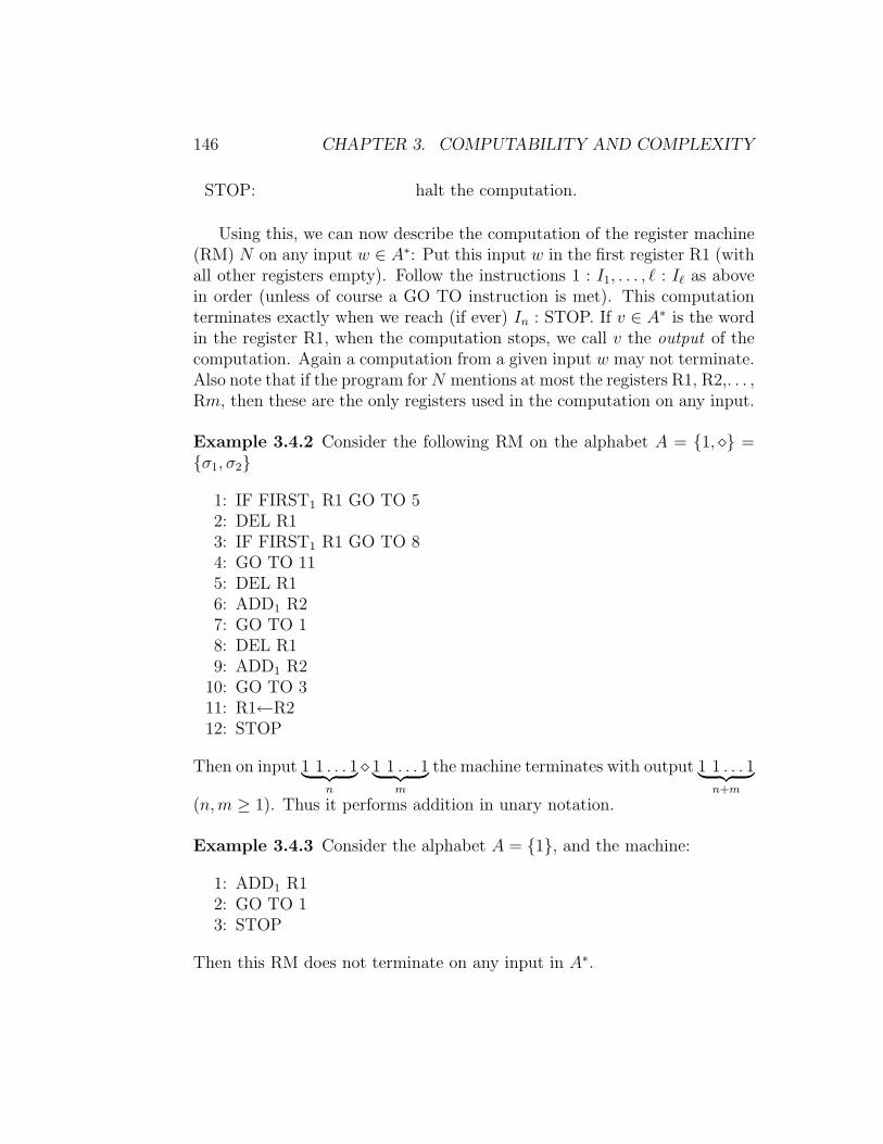
146 CHAPTER 3. COMPUTABILITY AND COMPLEXITY
STOP: halt the computation.
Using this, we can now describe the computation of the register machine(RM) N on any input w ∈ A∗: Put this input w in the first register R1 (withall other registers empty). Follow the instructions 1 : I1, . . . , ` : I` as abovein order (unless of course a GO TO instruction is met). This computationterminates exactly when we reach (if ever) In : STOP. If v ∈ A∗ is the wordin the register R1, when the computation stops, we call v the output of thecomputation. Again a computation from a given input w may not terminate.Also note that if the program for N mentions at most the registers R1, R2,. . . ,Rm, then these are the only registers used in the computation on any input.
Example 3.4.2 Consider the following RM on the alphabet A = {1, ¦} ={σ1, σ2}
1: IF FIRST1 R1 GO TO 52: DEL R13: IF FIRST1 R1 GO TO 84: GO TO 115: DEL R16: ADD1 R27: GO TO 18: DEL R19: ADD1 R2
10: GO TO 311: R1←R212: STOP
Then on input 1 1 . . . 1︸ ︷︷ ︸n
¦ 1 1 . . . 1︸ ︷︷ ︸m
the machine terminates with output 1 1 . . . 1︸ ︷︷ ︸n+m
(n,m ≥ 1). Thus it performs addition in unary notation.
Example 3.4.3 Consider the alphabet A = {1}, and the machine:
1: ADD1 R12: GO TO 13: STOP
Then this RM does not terminate on any input in A∗.

3.4. THE CHURCH-TURING THESIS 147
Although the TM and RM models of computation are quite different, itcan be shown that they are equivalent, in the sense that whatever can becomputed using one of the models can be computed with the other, andvice versa. More precisely, consider two finite alphabets A,B and a partialfunction f : A∗ → B∗, that is a function whose domain is a subset of A∗ andwhich takes values in B∗. (Normally, when we write g : X → Y we meanthat g is a total function with domain exactly X and values in Y . We willhowever use this notation below even if the domain of g is only a (possiblyproper) subset of X, but in this case we will explicitly state that g is partial.)
Definition 3.4.4 f : A∗ → B∗ is TM-computable if there is a finite alphabetC ⊇ A ∪ B and a Turing Machine M on C such that for each input w ∈A∗(⊆ C∗), M terminates on w iff w is the domain of f (i.e. f(w) is defined),and in that case the output of M on input w is f(w).
We define what it means for f to be RM-computable in a similar way.We can then show
Theorem 3.4.5 TM-computable = RM-computable.
This is a programming exercise and we will not discuss it in detail here.First, we show that given a RM N on an alphabet C, one can construct a TMM on the alphabet D = C ∪ {¦}, such that if we put w ∈ C∗ as input in Nand the same input w ∈ C∗ in M , then N terminates on w iff M terminateson w, and for such w the outputs of N and M are the same.
Specifically, we assume that all the registers mentioned in N are amongR1, R2,. . . , Rm. If R1,. . . , Rm, at some stage in the computation, containthe words w1, . . . , wm, respectively, then the idea is to represent their contentsby the word w1 ¦ w2 ¦ · · · ¦ wm¦ in the tape of the TM M , with the headscanning the leftmost symbol of w1 (or the first ¦ if w1 = θ). Then for eachinstruction of N we will introduce a block of entries in the table of M , whoseeffect on w1 ¦ w2 ¦ · · · ¦ wm¦ will correspond to the effect of the instructionof N on the corresponding register values. In the case of GOTO instructionsthis simulation will preserve the same flow of control.
Conversely, we can show that given a TM M on an alphabet C, onecan construct a RM N on some alphabet D ⊇ C such that again if we putw ∈ C∗ as input in M and N , then M terminates on w iff N terminateson w, and for such w the outputs of M and N on w are the same. Forexample, one way to do that is to take D = {σ0, σ1, . . . , σk} ∪ {Q0, . . . , Qm},

148 CHAPTER 3. COMPUTABILITY AND COMPLEXITY
if C = {σ1, . . . , σk} and M has set of states {Q0, . . . , Qm}. Now considera tape snapshot wQiav, which indicates that the head is in state Qi, scansthe symbol a (which could be the empty square, i.e. a = σ0), and to theleft of it is the word w ∈ {σ0, σ1, . . . , σk}∗ and to the right of it the wordv ∈ {σ0, σ1, . . . , σk}∗. Notice that at each stage of the computation of themachine M there will only be finitely many non-empty squares. Here w isthe word which represents from left-to-right the contents of the tape startingfrom the left-most non-empty square to the square just to the left of thesquare scanned by the head. In case every square to the left of the head isempty, w = θ. Similarly for v.
Example.
empty x y z?
︸ ︷︷ ︸w=xyσ0z
We can represent this tape snapshot in the register machine N by puttingw in R1, Qia in R2, and v in R3. Then for each entry (Qi, a,−,−,−) in thetable of M we can write a set of instructions (subroutine) for N such that theeffect of this entry on wQiav is the same as the effect of the corresponding setof instructions on the corresponding register values. In this way, we can showthat the notions of TM-computability and RM-computability are equivalent.
3.4.B The Church-Turing Thesis
As mentioned earlier, many alternative models of computation M have beenproposed over the years, and for each one we have a corresponding notion ofan M-computable function. Two common ones which we will not discuss,but which you may encounter later, are the Lambda Calculus and the theoryof Recursive Functions. Another one is the theory of cellular automata, anspecific example of which is Conway’s Game of Life. It turns out that in allthese cases, one can again prove that M-computable = TM-computable, soall these models are, in that sense, equivalent to the Turing machine model.
It is accepted today that the informal notion of algorithmic computabilityis represented correctly by the precise notion of TM-computability (= RM-computability = . . . ), in a way similar to the assertion that the formal ε-δdefinition of continuity of functions of a real variable represents accurately

3.5. UNIVERSAL MACHINES 149
the intuitive concept of continuity. This (extramathematical) assertion that“computability = TM-computability” is referred to as the Church-TuringThesis.
More explicitly, consider a partial function f : A∗ → B∗ (A,B finitealphabets). We call it intuitively computable if there is an algorithm whichfor each input w ∈ A∗ terminates (in finitely many steps) exactly when wis in the domain of f and in that case produces the output f(w). Then theChurch-Turing Thesis is the assertion:
intuitively computable = TM-computable.
We will simply say computable instead of TM-computable from now on.
Remark. Any decision problem (A,P ) may be identified with the (total)function f : A∗ → {Y,N}∗ given by f(w) = Y if w ∈ P and f(w) = N ifw 6∈ P . Thus (A,P ) is decidable iff f is computable.
3.5 Universal Machines
So far we have been discussing machines which represent the operation ofa single computer program. But what about a computer itself, i.e. a singlemachine which can execute any program? It turns out that our existingformalization is sufficient to deal with this more general case as well. Aftera bit of thought, this should come as no surprise, since after all the insideof a computer is just a program which sequentially reads and executes theinstructions of other programs. We will now describe how to formalize thisnotion.
To start with, we can effectively code the words in an arbitrary finitealphabet A = {σ1, . . . , σk} by using words in the binary alphabet {0, 1}.For example, if k = 22 we can use five letter words from {0, 1} to representeach individual symbol in A, and thus every word of length n from A canbe encoded as a word of length 5n in the binary alphabet. (We could evenuse the unary alphabet {1} instead of the binary alphabet, but this wouldrequire exponential increase in the length of the word if A has more than onesymbol. This does not affect computability issues, but it can certainly affectthe complexity issues discussed later.)
So let’s assume that we have fixed some simple method for encodingwords in a given alphabet A by binary words and refer to the binary word

150 CHAPTER 3. COMPUTABILITY AND COMPLEXITY
b(w) encoding the word w ∈ A∗ as the binary code of w. It is now not hardto see that given a TM M on A we can construct a TM M∗ on {0, 1} suchthat for each w ∈ A∗ the input-output behavior of M on w is exactly thesame on the input-output behavior of M∗ on b(w).
Thus, without any loss of generality, we can restrict ourselves to discussingTMs on the binary alphabet. Any such machine M is simply given by afinite table of 5-tuples which again can be easily coded as a word in thebinary alphabet. We call this the binary code of M and denote it by b(M).By carrying out a somewhat complicated programming project, one can nowconstruct a universal Turing Machine. This is a TM U on {0, 1} such thatfor any TM M on {0, 1} and any input w = {0, 1}∗, if we put b(M)∗w (where∗ = empty square) as input in U (so that in the beginning the head scansthe first symbol of b(M)), then U terminates on this input iff M terminateson w, and in this case their outputs are the same. So we have:
Theorem 3.5.1 (Existence of universal TM) We can construct a TMU on {0, 1} such that for any TM M on {0, 1} with binary code b(M), theinput-output behavior of U on b(M) ∗ w (w ∈ {0, 1}∗) is the same as theinput-output behavior of M on w.
Remark. The universal TM was conceived theoretically by Turing in the1930’s. Any personal computer today is essentially a practical implementa-tion of this idea.
3.6 The Halting Problem
We will now use theorem 3.5.1 to show that the so-called halting problem forTM is undecidable. This is precisely formulated as:
A = {0, 1}P = {b(M) : M is a TM on {0, 1} and M
terminates on the empty input}.(HALTING)
Theorem 3.6.1 (Turing) HALTING is undecidable.
Proof. Consider the universal TM U . For each x ∈ {0, 1}∗ consider theTM Ux which on the empty input first prints x ∗ x, moves the head over

3.7. UNDECIDABILITY OF THE VALIDITY PROBLEM 151
the first symbol of the first x, and then follows U . The table of Ux is easilyobtained from the table of U by adding some further entries depending on x.
Now, if HALTING were decidable, one could easily build a TM N0 on{0, 1} such that for any x ∈ {0, 1}∗, N0 on input x would terminate withoutput 0 if Ux terminated on the empty input, and N0 on input x wouldterminate with output 1 if Ux did not terminate on the empty input. Bychanging N0 a little, we could then construct a TM M0 on {0, 1} such thatif N0 on input x terminates with output 1, so does M0, but if N0 on inputx terminates with output 0, then M0 does not terminate in that input. Tosimplify the notation, let us write
M(w) ↓
if a TM M terminates on input w and
M(w) ↑
if it does not. Then we have for x ∈ {0, 1}∗
M0(x) ↓ ⇔ Ux(θ) ↑⇔ U(x ∗ x) ↑ .
In particular, for any TM M on {0, 1},
M0(b(M)) ↓ ⇔ U(b(M) ∗ b(M)) ↑⇔ M(b(M)) ↑
Putting M = M0 we get a contradiction, since it cannot be the case thatboth M0(b(M0)) ↑ and M0(b(M0)) ↓. a
Similarly one can of course prove that the corresponding halting problemfor RM is undecidable. More generally, given any programming language, itis impossible to design an algorithm that will decide whether an arbitraryprogram will terminate on a given input or not.
3.7 Undecidability of the Validity Problem
We have succeeded in showing that one problem—the halting problem—isundecidable, but the prospects are not good for applying the method we

152 CHAPTER 3. COMPUTABILITY AND COMPLEXITY
used to other problems, since it depends on the halting problem being a sortof “meta-problem” about computability. Fortunately, we can leverage thissuccess to show the undecidability of other problems, by using the methodof computable reductions, as follows.
Definition 3.7.1 Suppose (A,P ) and (B, Q) are two decision problems. A(total) function f : A∗ → B∗ is a (computable) reduction of P to Q if f iscomputable and for any w ∈ A∗,
w ∈ P ⇔ f(w) ∈ Q.
Notice that if P is reduced to Q via f and Q is decidable, so that thereis a total computable function g : B∗ → {Y,N}∗ such that v ∈ Q ⇒ g(v) =Y, v 6∈ Q ⇒ g(v) = N , then g◦f = h is computable and w ∈ P ⇒ h(w) = Y ,w 6∈ P ⇒ h(w) = N . Thus P is decidable as well.
So if P can be reduced to Q and Q is decidable, then P is decidable. Thisobservation provides a general method for showing that decision problemsare undecidable. Specifically, to show that (B, Q) is undecidable, choosean appropriate problem (A,P ) that is known to be undecidable, and finda reduction of P to Q. For then if (B, Q) were decidable, so would (A,P )be, which we know is not the case. We will apply this method to show theundecidability of the validity problem for an appropriate language L.
Theorem 3.7.2 (Church) There is a finite language L such that the deci-sion problem VALIDITYL is undecidable.
Proof. First consider a variation of the halting problem, HALTINGU . Thisis simply the halting problem for the universal TM U . It consists of allw ∈ {0, 1}∗ for which U(w) ↓. Since for any TM M on {0, 1}∗, M(θ) ↓ iffU(b(M) ∗ θ) ↓ iff U(b(M)) ↓, clearly HALTINGU is also undecidable.
Say the states of U are {Q0, Q1, . . . , Qm}. We take L to consist of thefollowing symbols:
0 : constantS : unary function< : binary relationH : binary relation
T∗, T0, T1 : binary relationsR0, . . . , Rm : unary relations.

3.7. UNDECIDABILITY OF THE VALIDITY PROBLEM 153
Intuitively, we have in mind the following interpretation for these:
(i) 0, S, < will be the 0, successor and order on 〈Z, 0, S,<〉.(ii) Variables will vary over Z. They will represent both the time (i.e. stage
in the computation), when restricted to ≥ 0 values (so 0 will be thebeginning, 1 the next step, 2 the next one, etc.), and also the locationof a square on the tape.
· · · · · ·-2 -1 0 1 2
(iii) H(t, x) will be true iff t, x ∈ Z, t ≥ 0 and the head at time t scans thesquare x.
(iv) T∗(t, x) will be true iff t, x ∈ Z, t ≥ 0 and the tape at time t contains∗ (i.e. is empty) at the square x, and similarly for T0 and T1.
(v) Ri(t) will be true iff t ∈ Z, t ≥ 0, and at time t the machine is in stateQi.
We will now assign to each w ∈ {0, 1}∗ a sentence σw in L such that
U(w) ↓ iff σw is valid.
It will be clear from our construction that the map w 7→ σw is computable.Thus it will follow that HALTINGU can be reduced to VALIDITYL, soVALIDITYL must be undecidable.
We will first construct some preliminary sentences in L:
(i) Z is the conjunction of the following sentences:
∀x(¬x < x)
∀x∀y∀z(x < y ∧ y < z ⇒ x < z)
∀x∀y(x < y ∨ x = y ∨ y < x)
∀x∃y(S(y) = x)
∀x(x < S(x))
∀x∀y(x < y ⇒ y = S(x) ∨ S(x) < y)
(expressing the usual properties of 〈Z, 0, S,<〉).

154 CHAPTER 3. COMPUTABILITY AND COMPLEXITY
(ii) NOCONFLICT is the conjunction of the following sentences:
∀t(0 = t ∨ 0 < t ⇒ R0(t) ∨ · · · ∨Rm(t))
∀t(0 = t ∨ 0 < t ⇒ ¬Ri(t) ∨ ¬Ri′(t)), 0 ≤ i < i′ ≤ m
∀t(0 = t ∨ 0 < t ⇒ ∃xH(t, x))
∀t∀x∀x′((0 = t ∨ 0 < t) ∧ x 6= x′ ⇒ ¬H(t, x) ∨ ¬H(t, x′))
∀t∀x(0 = t ∨ 0 < t ⇒ T∗(t, x) ∨ T0(t, x) ∨ T1(t, x))
∀t∀x(0 = t ∨ 0 < t ⇒ (¬T∗(t, x) ∨ ¬T0(t, x)))
∀t∀x(0 = t ∨ 0 < t ⇒ (¬T0(t, x) ∨ ¬T1(t1, x))
∀t∀x(0 = t ∨ 0 < t ⇒ (¬T1(t, x) ∨ ¬T∗(t, x))
expressing that at each time t, M is in exactly one state, and scansexactly one square, and for each time t and each square x there isexactly one symbol on that square (possibly empty).
(iii) STARTw is the conjunction of the following sentences, where w =w0 . . . wn−1 with wi ∈ {0, 1}, and we use the abbreviation
i = S(S(. . . S(0)) . . . )
(i times) for all 0 ≤ i ∈ Z:
R0(0)
H(0, 0)
Tw(i)(0, i), 0 ≤ i < n
∀x(n < x ∨ n = x ⇒ T∗(x))
∀x(x < 0 ⇒ T∗(x))
(expressing that the machine starts in state Q0 with the head on the0th square and on the input w).
(iv) NONSTOP is the sentence
∀t(0 = t ∨ 0 < t ⇒ ¬Rm(t))
expressing that the machine does not stop.
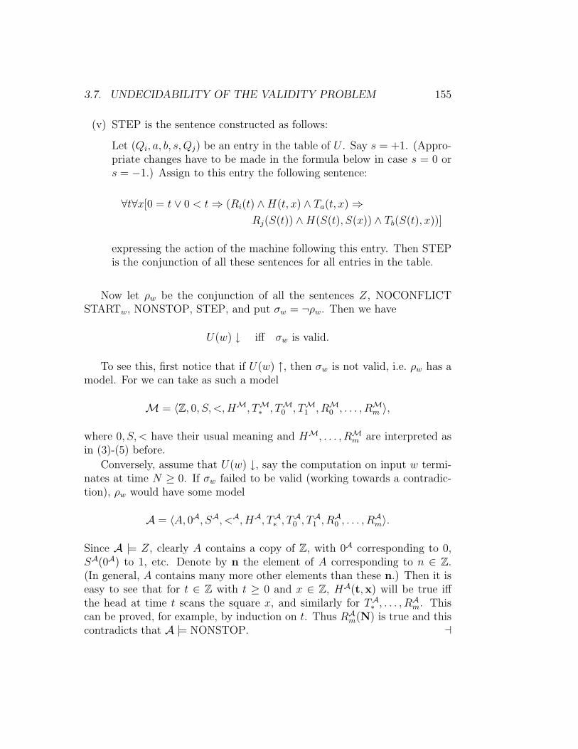
3.7. UNDECIDABILITY OF THE VALIDITY PROBLEM 155
(v) STEP is the sentence constructed as follows:
Let (Qi, a, b, s, Qj) be an entry in the table of U . Say s = +1. (Appro-priate changes have to be made in the formula below in case s = 0 ors = −1.) Assign to this entry the following sentence:
∀t∀x[0 = t ∨ 0 < t ⇒ (Ri(t) ∧H(t, x) ∧ Ta(t, x) ⇒Rj(S(t)) ∧H(S(t), S(x)) ∧ Tb(S(t), x))]
expressing the action of the machine following this entry. Then STEPis the conjunction of all these sentences for all entries in the table.
Now let ρw be the conjunction of all the sentences Z, NOCONFLICTSTARTw, NONSTOP, STEP, and put σw = ¬ρw. Then we have
U(w) ↓ iff σw is valid.
To see this, first notice that if U(w) ↑, then σw is not valid, i.e. ρw has amodel. For we can take as such a model
M = 〈Z, 0, S, <,HM, TM∗ , TM
0 , TM1 , RM
0 , . . . , RMm 〉,
where 0, S, < have their usual meaning and HM, . . . , RMm are interpreted as
in (3)-(5) before.
Conversely, assume that U(w) ↓, say the computation on input w termi-nates at time N ≥ 0. If σw failed to be valid (working towards a contradic-tion), ρw would have some model
A = 〈A, 0A, SA, <A, HA, TA∗ , TA
0 , TA1 , RA
0 , . . . , RAm〉.
Since A |= Z, clearly A contains a copy of Z, with 0A corresponding to 0,SA(0A) to 1, etc. Denote by n the element of A corresponding to n ∈ Z.(In general, A contains many more other elements than these n.) Then it iseasy to see that for t ∈ Z with t ≥ 0 and x ∈ Z, HA(t,x) will be true iffthe head at time t scans the square x, and similarly for TA
∗ , . . . , RAm. This
can be proved, for example, by induction on t. Thus RAm(N) is true and this
contradicts that A |= NONSTOP. a
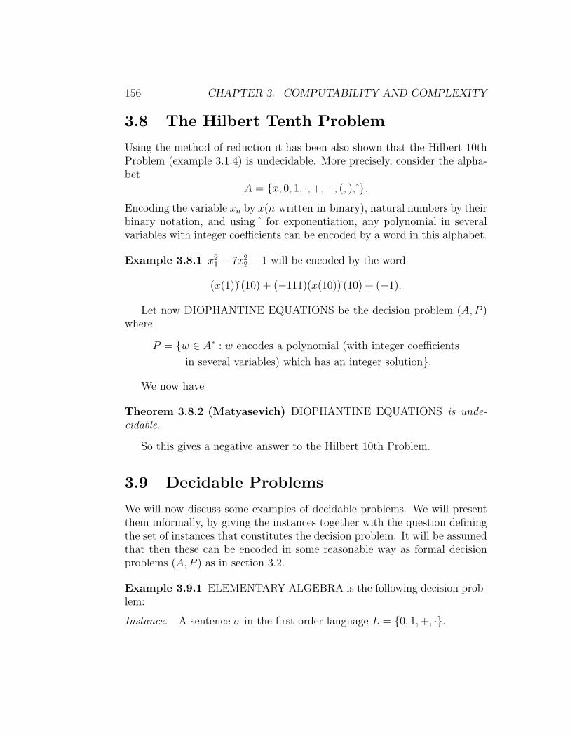
156 CHAPTER 3. COMPUTABILITY AND COMPLEXITY
3.8 The Hilbert Tenth Problem
Using the method of reduction it has been also shown that the Hilbert 10thProblem (example 3.1.4) is undecidable. More precisely, consider the alpha-bet
A = {x, 0, 1, ·, +,−, (, ), }.Encoding the variable xn by x(n written in binary), natural numbers by theirbinary notation, and using ˆ for exponentiation, any polynomial in severalvariables with integer coefficients can be encoded by a word in this alphabet.
Example 3.8.1 x21 − 7x2
2 − 1 will be encoded by the word
(x(1)) (10) + (−111)(x(10)) (10) + (−1).
Let now DIOPHANTINE EQUATIONS be the decision problem (A,P )where
P = {w ∈ A∗ : w encodes a polynomial (with integer coefficients
in several variables) which has an integer solution}.
We now have
Theorem 3.8.2 (Matyasevich) DIOPHANTINE EQUATIONS is unde-cidable.
So this gives a negative answer to the Hilbert 10th Problem.
3.9 Decidable Problems
We will now discuss some examples of decidable problems. We will presentthem informally, by giving the instances together with the question definingthe set of instances that constitutes the decision problem. It will be assumedthat then these can be encoded in some reasonable way as formal decisionproblems (A,P ) as in section 3.2.
Example 3.9.1 ELEMENTARY ALGEBRA is the following decision prob-lem:
Instance. A sentence σ in the first-order language L = {0, 1, +, ·}.

3.9. DECIDABLE PROBLEMS 157
Question. Is σ true in 〈R, 0, 1, +, ·〉, i.e. is σ ∈ Th(R, 0, 1, +, ·)?Tarski in 1949 has shown that ELEMENTARY ALGEBRA is decidable.
Remark. On the other hand, if we consider the corresponding problem ELE-MENTARY ARITHMETIC for Th(N , 0, S, +, ·, <), then Church has shownin the 1930’s that it is undecidable (this also follows easily from 3.8.2).
Example 3.9.2 SATISFIABILITY is the following decision problem:
Instance. A finite set U = {u1, . . . , uk} of propositional variables and C ={c1, . . . , cm} a finite set of clauses ci = {`i,1, . . . , `i,ni
}, where each `i,j is aliteral from U , i.e. a variable in U or its negation. (As usual we write ui
instead of ¬ui in this context.)
Question. Is C satisfiable (i.e. is there a valuation ν : U → {T, F} whichmakes every clause ci true, recalling that the clause ci as above representsthe disjunction `i,1 ∨ · · · ∨ `i,ni
)?
Using truth tables it is clear that SATISFIABILITY is decidable.
Example 3.9.3 TRAVELING SALESMAN is the following decision prob-lem:
Instance. A finite set {c1, . . . , cm} of “cities”, a distance function d(ci, cj) ∈{1, 2, . . . } for i 6= j, and a bound B ∈ {1, 2, . . . }.Question. Is there a tour of all the cities with total length ≤ B, i.e. anordering cπ(1), cπ(2), . . . , cπ(m) of {c1, . . . , cm} such that
m−1∑i=1
d(cπ(i), cπ(i+1)) + d(cπ(m), cπ(1)) ≤ B?
Again, by listing all possible orderings and calculating the above sum foreach one of these, it is trivial to see that this problem is decidable.
Example 3.9.4 PRIMES is the following decision problem:
Instance. An integer n ≥ 2.
Question. Is n prime?
This is also decidable as we can go through all the integers between 2 andn− 1 and check whether they divide n.

158 CHAPTER 3. COMPUTABILITY AND COMPLEXITY
3.10 The Class PWe have so far been discussing what problems are computable in princi-ple. However, a question of more practical interest is the following: given aproblem which is computable, can we compute it efficiently? The study ofefficiency is also called computational complexity. We will concentrate hereon time complexity (how long it takes to solve the problem), but one can alsodiscuss, for example, space complexity (how much “memory” storage is usedin solving it). A natural measure of time complexity for us is the number ofsteps in the computation of a TM that decides a given problem.
Since different problems require different amounts of input, in order tocompare the complexities of different algorithms and problems, we must mea-sure complexity as a function of the input size. In addition, with computerspeeds increasing rapidly, small instances of a problem can usually be solvedno matter how difficult the problem is. For this reason, and also to eliminatethe effect of “overhead” time, we will consider only the asymptotic complex-ity as the size of the input increases. First we recall the “big-O notation,”which gives a rigorous way of comparing asymptotic growth rates.
Definition 3.10.1 Given two functions f, g : N→ N we define
f = O(g) iff ∃n0 ∃C ∀n ≥ n0(f(n) ≤ Cg(n)).
For example, if p(n) is a polynomial, then p(n) = O(nd) for large enough d.
Definition 3.10.2 Given any T : N → N, we let TIME(T ) consist of alldecision problems (A,P ) which can be decided by a TM in time t for somet = O(T ).
More precisely, a decision problem (A,P ) is in TIME(T ) if there is t =O(T ) and a TM M on some alphabet B ⊇ A∪{Y,N} such that for w ∈ A∗:
(i) w ∈ P ⇒ on input w, M halts in ≤ t(|w|) steps with output Y .
(ii) w 6∈ P ⇒ on input w, M halts in ≤ t(|w|) steps with output N
(here |w| = length of the word w).What sort of growth rate should we require of an algorithm to consider
it manageable? After all, we must expect the time to increase somewhatwith the input size. It turns out that the major distinctions in complexityare between “polynomial time” algorithms and faster-growing ones, such asexponentials.

3.10. THE CLASS P 159
Definition 3.10.3 A decision problem is in the class P (or it is polynomi-ally decidable) if it is TIME(nd) for some d ≥ 0, i.e. it can be decided inpolynomial time.
Problems in the class P are considered tractable (efficiently decidable)and the others intractable. It is clear that the class P provides an upperlimit for problems that can be algorithmically solved in realistic terms. If aproblem is in P , however, it does not necessarily mean that an algorithm forit can be practically implemented, for example, it could have time complexityof the order of n1,000,000 or of the order n3 but with enormous coefficients.However, most natural problems that have been shown to be polynomiallydecidable have been found to have efficient (e.g., very low degree) algorithms.Moreover, the class of problems in P behaves well mathematically, and isindependent of the model of computation, since any two formal models ofcomputation can be mutually simulated within polynomial time.
Remark. Time complexity as explained here is a worst case analysis. If aproblem P is intractable, then there is no polynomial time algorithm whichfor all n and all inputs of length n will decide P . But one can still search forapproximate algorithms that work well on the average or for most practical(e.g., small) instances of the problem or give the correct answer with highprobability, etc.
Example 3.10.4 ELEMENTARY ALGEBRA is intractable (Fisher-Rabin1974). In fact it is in TIME(22cn
) for some c > 0 but not in TIME(2dn) forany d > 0; that is, it is super-exponential.
Example 3.10.5 LINEAR PROGRAMMING is the decision problem givenby:
Instance. An integer matrix (vij) for 1 ≤ i ≤ m and 1 ≤ j ≤ n, along withinteger vectors D = (di)
mi=1 and C = (cj)
nj=1, and an integer B.
Question. Is there a rational vector X = (xj)nj=1 such that
∑nj=1 vijxj ≤ di,
for 1 ≤ i ≤ m, and∑n
j=1 cjxj ≥ B?
LINEAR PROGRAMMING turns out to be in P (Khachian, 1979).

160 CHAPTER 3. COMPUTABILITY AND COMPLEXITY
3.11 The Class NP and the P = NP Problem
Although a large class of problems have been classified as tractable or in-tractable, there is a vast collection of decision problems, many of them ofgreat practical importance, that are widely assumed to be intractable butno one until now has been able to demonstrate it. These are the so-calledNP-complete problems. In order to introduce these problems, we must firstdefine the class NP of non-deterministic polynomial decision problems.
Definition 3.11.1 Let (A,P ) be a decision problem. We say that (A,P ) isin the class NP if there is a TM M on an alphabet B ⊇ A ∪ {Y, N} and apolynomial p(n) such that for any w ∈ A∗:
w ∈ P ⇔ ∃v ∈ B∗ such that |v| ≤ p(|w|) and on input w ∗ v, Mstops with output Y after at most p(|w|) many steps.
In other words, w ∈ P iff there is a “guess” v, of length bounded by apolynomial in the length of w, such that w together with v pass a polynomialacceptance test. (This can be also viewed as a non-deterministic polynomialtime algorithm.)
Example 3.11.2 SATISFIABILITY is in NP , since if we can guess a truthassignment, we can verify that it satisfies the given set of clauses in polyno-mial time.
Example 3.11.3 Similarly, TRAVELING SALESMAN is in NP , since ifwe guess the order of the set of cities, we can calculate whether the lengthof the tour is ≤ B in polynomial time.
In fact a vast number of problems like these, which involve some kind ofsearch, are in NP .
Remark. Clearly P ⊆ NP ⊆ ⋃d TIME(2nd
).
Problem. A famous problem in theoretical computer science is whether
P = NP ,
that is, whether any problem with an efficient nondeterministic algorithmalso has an efficient deterministic algorithm. This is known, unsurprisingly,as the P = NP Problem. Recently the Clay Mathematics Institute includedthe P = NP Problem as one of its seven Millenium Prize Problems, offering$1,000,000 for its solution! The prevailing assumption today is that P 6= NP .

3.12. NP-COMPLETE PROBLEMS 161
3.12 NP-Complete Problems
We can get a better understanding of the P = NP problem by discussingthe notion of an NP-complete problem. The NP-complete problems formsort of a “core” of the “most difficult” problems in NP . Recall the conceptof a computable reduction (definition 3.7.1). We adapt this to the setting ofcomplexity as follows:
Definition 3.12.1 A (total) function f : A∗ → B∗, where A,B are finitealphabets, is polynomial-time computable if there is a TM M on a finitealphabet C ⊇ A ∪B, and a polynomial p, such that for every input w ∈ A∗,M terminates on at most p(|w|) steps with output f(w).
Unsurprisingly, a polynomial-time reduction is a computable reductionwhich is in addition polynomial-time computable. We now say that
Definition 3.12.2 A decision problem (B, Q) isNP-complete if it is inNP ,and for every NP problem (A,P ) there is a polynomial-time reduction of Pto Q. (That is, there is a polynomial-time computable function f : A∗ → B∗
such that w ∈ P if and only if f(w) ∈ Q.)
An NP-complete problem is in some sense a hardest possible problemin NP . For example, it is clear that if (B, Q) is in P and (A,P ) can bepolynomial-time reduced to Q, then also (A,P ) is in P . It therefore followsthat if any NP-complete problem is in P , then P = NP . Thus the P = NPquestion is equivalent to the question of whether any given NP-completeproblem is in P .
It is clear from the definition that all NP-complete problems are “equiv-alent” in some sense, since each one can be reduced to the other by apolynomial-time computable function. We have not yet established how-ever that there are any NP-complete problems. This was first shown byCook and Levin in 1971.
Theorem 3.12.3 (Cook, Levin) SATISFIABILITY is NP-complete.
Karp in 1972 has shown that TRAVELING SALESMAN and many othercombinatorial problems are NP-complete, and since that time hundreds ofothers have been discovered in many areas of mathematics and computerscience.

162 CHAPTER 3. COMPUTABILITY AND COMPLEXITY
We will give a proof of this theorem shortly, but first let us say a fewthings about the complexity of PRIMES, because it occupies a special placeamong “difficult” problems. Given a decision problem (A,P ), its complementis the decision problem (A,∼ P ), where ∼ P = A∗ \ P . It is clear that aproblem is decidable (or in P) iff its complement is decidable (or in P), butit is unknown whether a problem is in NP iff its complement is NP .
We denote by “co-NP” the class of problems whose complements are inNP . Thus P ⊆ NP∩co-NP , but whether NP = co-NP is unknown. Nowit is easy to see that PRIMES in co-NP . (In precisely formulating PRIMESwe assume that every positive integer is represented by its binary notation.If numbers were represented in unary notation, then clearly PRIMES wouldbe in P .) With some work, using some elementary number theory, it can beshown that PRIMES is also in NP . Thus
PRIMES ∈ NP ∩ co-NP .
Miller in 1976 has shown that if one assumes a widely believed but stillunproven hypothesis, the so-called Generalized Riemann Hypothesis, thenactually PRIMES is in P , but it is still unknown whether PRIMES is actuallyin P . (Addendum: In 2002 Agrawal, Kayal and Saxena proved that PRIMESis indeed in P .)
Proof of 3.12.3. The proof is a variation of that of 3.7.2.To fix a formal encoding of the satisfiability problem, we simply view
each instance as a formula in propositional logic in conjunctive normal form(cnf), and which can thus be viewed as a word in the alphabet
C = {p, 0, 1,¬,∧,∨, (, )},
where we write pn, with n in binary, instead of the propositional variable pn.Consider now an arbitrary decision problem (A,P ) which is in the class
NP . We will find a polynomial-time computable map f : A∗ → C∗ suchthat, for each w ∈ A∗, f(w) is a formula in cnf and
w ∈ P ⇔ f(w) is satisfiable.
By a slight reformulation of the definition of what it means to be in theclass NP , we can find an alphabet B ⊇ A, a polynomial p(n) > n and aTM M on B with states {Q0, . . . , Qm} (Q0 is the start and Qm is the stop

3.12. NP-COMPLETE PROBLEMS 163
state), such that all the entries in the table of M that begin with Qm are ofthe form (Qm, b, b, 0, Qm), and we have for any w = a0a1 . . . an−1 ∈ A∗:
w ∈ P iff there is an input
?
Q0
a0 a1 an−1 ∗−p(n) 0 1 n− 1 n p(n)
· · · · · · · · ·
in which ai is in square i, 0 ≤ i ≤ n− 1, square n is empty, as are all squaresj < 0 and j > p(n) (but some symbols in B are possibly occupying somesquares between n + 1 and p(n)), and on which M terminates in at mostp(n) many steps (and thus at each step of the computation the machine onlyvisits squares with index −p(n) ≤ j ≤ p(n)).
Let A = {σ1, . . . , σK}, B = {σ1, . . . , σK , σK+1, . . . , σL}, and finally let σ0
denote the empty square.Associate with M and each n = 0, 1, 2, . . . the following list of proposi-
tional variables:
(i) Ri,k, 0 ≤ i ≤ p(n), 0 ≤ k ≤ m,
(ii) Hi,j, 0 ≤ i ≤ p(n), −p(n) ≤ j ≤ p(n),
(iii) Ti,j,`, 0 ≤ i ≤ p(n), −p(n) ≤ j ≤ p(n), 0 ≤ ` ≤ L.
The intended meanings of these variables are as follows:
(i) Ri,k being true means that at time i the machine is in state Qk.
(ii) Hi,j being true means that at time i the head scans square j.
(iii) Ti,j,` being true means that at time i the tape contains σ` at square j.
(We can of course view these propositional variables as part of our standardlist p0, p1, p2, . . . .)
Consider now the following clauses in these variables, associated to eachw = σk0σk1 . . . σkn−1 ∈ A∗, 1 ≤ ki ≤ K:
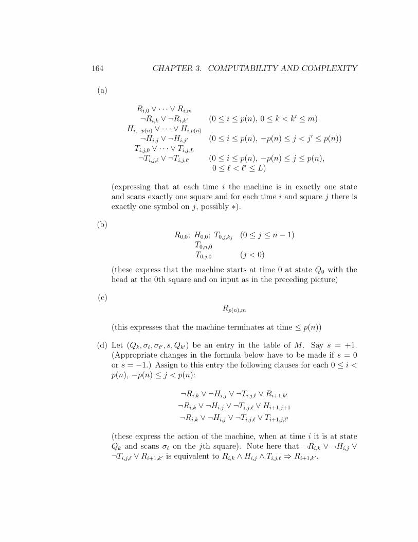
164 CHAPTER 3. COMPUTABILITY AND COMPLEXITY
(a)
Ri,0 ∨ · · · ∨Ri,m
¬Ri,k ∨ ¬Ri,k′ (0 ≤ i ≤ p(n), 0 ≤ k < k′ ≤ m)Hi,−p(n) ∨ · · · ∨Hi,p(n)
¬Hi,j ∨ ¬Hi,j′ (0 ≤ i ≤ p(n), −p(n) ≤ j < j′ ≤ p(n))Ti,j,0 ∨ · · · ∨ Ti,j,L
¬Ti,j,` ∨ ¬Ti,j,`′ (0 ≤ i ≤ p(n), −p(n) ≤ j ≤ p(n),0 ≤ ` < `′ ≤ L)
(expressing that at each time i the machine is in exactly one stateand scans exactly one square and for each time i and square j there isexactly one symbol on j, possibly ∗).
(b)
R0,0; H0,0; T0,j,kj(0 ≤ j ≤ n− 1)
T0,n,0
T0,j,0 (j < 0)
(these express that the machine starts at time 0 at state Q0 with thehead at the 0th square and on input as in the preceding picture)
(c)
Rp(n),m
(this expresses that the machine terminates at time ≤ p(n))
(d) Let (Qk, σ`, σ`′ , s, Qk′) be an entry in the table of M . Say s = +1.(Appropriate changes in the formula below have to be made if s = 0or s = −1.) Assign to this entry the following clauses for each 0 ≤ i <p(n), −p(n) ≤ j < p(n):
¬Ri,k ∨ ¬Hi,j ∨ ¬Ti,j,` ∨Ri+1,k′
¬Ri,k ∨ ¬Hi,j ∨ ¬Ti,j,` ∨Hi+1,j+1
¬Ri,k ∨ ¬Hi,j ∨ ¬Ti,j,` ∨ Ti+1,j,`′
(these express the action of the machine, when at time i it is at stateQk and scans σ` on the jth square). Note here that ¬Ri,k ∨ ¬Hi,j ∨¬Ti,j,` ∨Ri+1,k′ is equivalent to Ri,k ∧Hi,j ∧ Ti,j,` ⇒ Ri+1,k′ .

3.12. NP-COMPLETE PROBLEMS 165
Finally, let f(w) be the conjunction of all the formulas (clauses) given in(a), (b), (c), (d). It is easy to check that f is a polynomial-time computablefunction. We verify that w ∈ P ⇔ f(w) is satisfiable.
If w ∈ P , then we can find an input as in the previous picture with theproperties stated there and we assign truth values to the variables accordingto their intended meaning in this computation associated with that input.This valuation clearly satisfies all the clauses of f(w).
Conversely, assume a valuation ν satisfies all the clauses in f(w). Becauseν satisfies all the clauses in (a), (b), for each −p(n) ≤ j ≤ p(n) there is aunique σk(j) (0 ≤ k(j) ≤ L) with ν(T0,j,k(j)) = T . Consider the input for Mthat has σk(j) in the jth square. Because kj = k(j) for 0 ≤ j ≤ n − 1 andk(n) = 0, this is exactly an input as in the preceding picture. If we start Mon that input then it is easy to see, since ν satisfies all the clauses in (a),(d), that for all 0 ≤ i ≤ p(n), ν(Ri,k) = T iff at time i in this computationthe machine is in state Qk, and similarly for Hi,j and Ti,j,`. This is provedby induction on i. But then, since ν satisfies (c), we must have that thecomputation of M on that inputs stops in at most p(n) steps, so w ∈ P . a

166 CHAPTER 3. COMPUTABILITY AND COMPLEXITY

Appendix A
A list of tautologies andequivalences in propositionallogic
A.1 Tautologies
1. ((A ∧ A) ⇔ A)
2. ((A ∨ A) ⇔ A)
3. ((A ∧B) ⇔ (B ∧ A))
4. ((A ∨B) ⇔ (B ∨ A))
5. ((A ∧ (B ∧ C)) ⇔ ((A ∧B) ∧ C))
6. ((A ∨ (B ∨ C)) ⇔ ((A ∨B) ∨ C))
7. ((A ∧ (B ∨ C)) ⇔ ((A ∧B) ∨ (A ∧ C)))
8. ((A ∨ (B ∧ C)) ⇔ ((A ∨B) ∧ (A ∨ C)))
9. ((A ∧ (A ∨B)) ⇔ A)
10. ((A ∨ (A ∧B)) ⇔ A)
11. (¬(A ∨B) ⇔ (¬A ∧ ¬B))
167

168 APPENDIX A. TAUTOLOGIES AND EQUIVALENCES
12. (¬(A ∧B) ⇔ (¬A ∨ ¬B))
13. ((A ∧ >) ⇔ A), > any tautology
14. ((A∨ ⊥) ⇔ A), ⊥ any contradictory wff
15. ((A∧ ⊥) ⇔⊥)
16. ((A ∨ >) ⇔ >)
17. ((A ⇒ B) ⇔ (¬B ⇒ ¬A))
18. (A ∨ ¬A)
19. (A ⇒ A)
20. (A ⇔ A)
21. (¬¬A ⇔ A)
22. (A ⇒ (A ∨B))
23. ((A ∧B) ⇒ A)
24. (((A ⇒ B) ∧ A) ⇒ B)
25. (((A ⇒ B) ∧ ¬B) ⇒ ¬A)
26. ((¬A ⇒ A) ⇔ A)
27. (¬A ⇒ (A ⇒ B))
28. (A ∨ (A ⇒ B))
29. (A ⇒ (B ⇒ A))
30. (((A ⇒ B) ∧ (B ⇒ C)) ⇒ (A ⇒ C))
31. ((A ⇒ B) ∨ (C ⇒ A))
32. ((A ⇒ B) ∨ (¬A ⇒ B))
33. ((A ⇒ B) ∨ (A ⇒ ¬B))
34. ((A ⇒ B) ⇒ ((B ⇒ C) ⇒ (A ⇒ C)))

A.2. EQUIVALENCES 169
35. (¬A ⇒ (¬B ⇔ (B ⇒ A)))
36. ((A ⇒ B) ⇒ (((A ⇒ C) ⇒ B) ⇒ B))
A.2 Equivalences
All the formulas in each row are equivalent to each other.
37. (A ⇒ B), (¬A ∨B), (¬B ⇒ ¬A), ((A ∧B) ⇔ A), ((A ∨B) ⇔ B)
38. ¬(A ⇒ B), (A ∧ ¬B)
39. (A ⇔ B), ((A ∧B) ∨ (¬A ∧ ¬B)), ((¬A ∨B) ∧ (¬B ∨ A))
40. (A ⇔ B), ((A ⇒ B) ∧ (B ⇒ A)), (¬A ⇔ ¬B), (B ⇔ A)
41. (A ⇔ B), ((A ∨B) ⇒ (A ∧B))
42. ¬(A ⇔ B), (A ⇔ ¬B), (¬A ⇔ B)
43. A, ¬¬A, (A ∧ A), (A ∨ A), (A ∨ (A ∧B)), (A ∧ (A ∨B))
44. A, (¬A ⇒ A), ((A ⇒ B) ⇒ A), ((B ⇒ A) ∧ (¬B ⇒ A))
45. A, (A ∧ >), (A∨ ⊥), (A ⇔ >), (> ⇒ A)
46. ¬A, (A ⇒ ¬A), ((A ⇒ B) ∧ (A ⇒ ¬B))
47. ¬A, (A ⇒⊥), (A ⇔⊥)
48. ⊥, (A∧ ⊥), (A ⇔ ¬A)
49. >, (A ∨ >), (A ⇒ >), (⊥⇒ A)
50. (A ∧B), (B ∧ A), (A ∧ (¬A ∨B)), ¬(A ⇒ ¬B)
51. (A ∨B), (B ∨ A), (A ∨ (¬A ∧B)), (¬A ⇒ B), ((A ⇒ B) ⇒ B)
52. (A ⇒ (B ⇒ C)), ((A ∧ B) ⇒ C), (B ⇒ (A ⇒ C)), ((A ⇒ B) ⇒(A ⇒ C))
53. (A ⇒ (B ∧ C)), ((A ⇒ B) ∧ (A ⇒ C))

170 APPENDIX A. TAUTOLOGIES AND EQUIVALENCES
54. (A ⇒ (B ∨ C)), ((A ⇒ B) ∨ (A ⇒ C))
55. ((A ∧B) ⇒ C), ((A ⇒ C) ∨ (B ⇒ C))
56. ((A ∨B) ⇒ C), ((A ⇒ C) ∧ (B ⇒ C))
57. (A ⇔ (B ⇔ C)), ((A ⇔ B) ⇔ C)
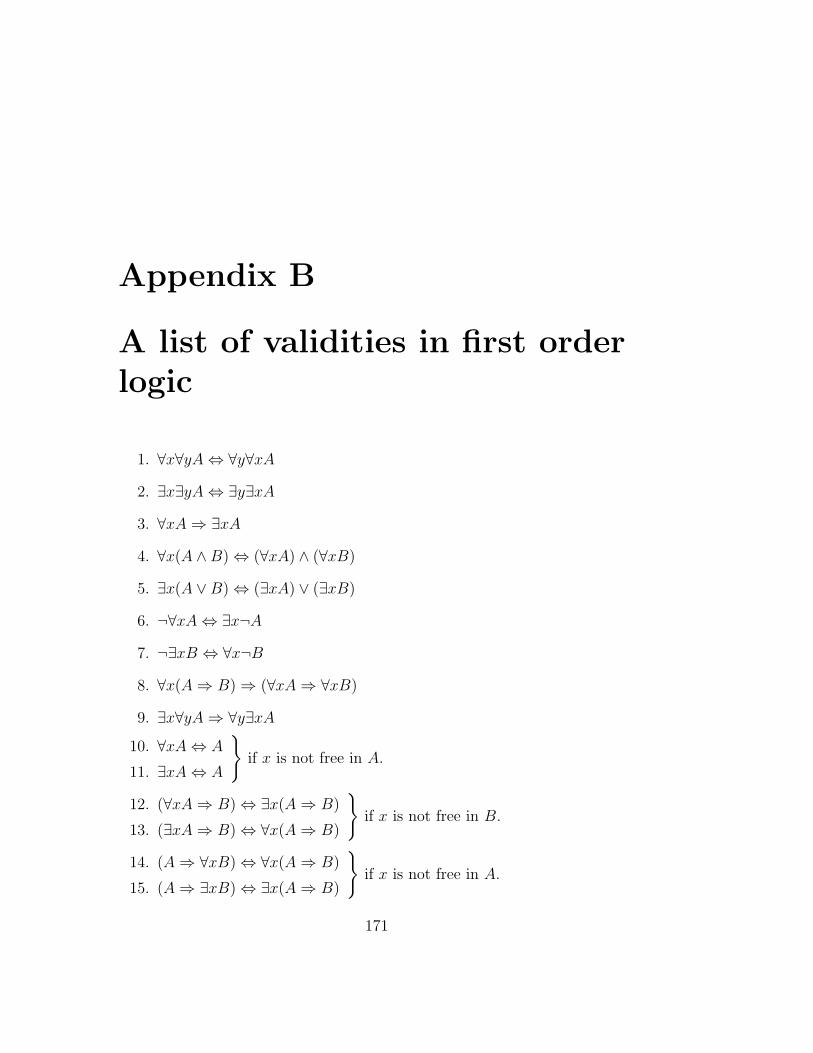
Appendix B
A list of validities in first orderlogic
1. ∀x∀yA ⇔ ∀y∀xA
2. ∃x∃yA ⇔ ∃y∃xA
3. ∀xA ⇒ ∃xA
4. ∀x(A ∧B) ⇔ (∀xA) ∧ (∀xB)
5. ∃x(A ∨B) ⇔ (∃xA) ∨ (∃xB)
6. ¬∀xA ⇔ ∃x¬A
7. ¬∃xB ⇔ ∀x¬B
8. ∀x(A ⇒ B) ⇒ (∀xA ⇒ ∀xB)
9. ∃x∀yA ⇒ ∀y∃xA
10. ∀xA ⇔ A
11. ∃xA ⇔ A
}if x is not free in A.
12. (∀xA ⇒ B) ⇔ ∃x(A ⇒ B)
13. (∃xA ⇒ B) ⇔ ∀x(A ⇒ B)
}if x is not free in B.
14. (A ⇒ ∀xB) ⇔ ∀x(A ⇒ B)
15. (A ⇒ ∃xB) ⇔ ∃x(A ⇒ B)
}if x is not free in A.
171

172 APPENDIX B. VALIDITIES IN FIRST ORDER LOGIC
16. x = x
17. (x = y ∧ y = z) ⇒ (x = z)
18. x = y ⇒ y = x
19. (y1 = z1 ∧ · · · ∧ yn = zn) ⇒ (f(y1, . . . , yn) = f(z1, . . . , zn))(f any n-ary function symbol)
20. (y1 = z1 ∧ · · · ∧ ym = zm) ⇒ (R(y1, . . . , ym) ⇔ R(z1, . . . , zm))(R any m-ary relation symbol)