
Lecture Notes in Information Theory Part I - Department of
327
Information Theory for Single-User Systems by Fady Alajaji † and Po-Ning Chen ‡ † Department of Mathematics & Statistics, Queen’s University, Kingston, ON K7L 3N6, Canada Email: [email protected] ‡ Department of Electrical Engineering Institute of Communication Engineering National Chiao Tung University 1001, Ta Hsueh Road Hsin Chu, Taiwan 30056 Republic of China Email: [email protected] June 21, 2016
Transcript of Lecture Notes in Information Theory Part I - Department of

Information Theory for Single-User Systems
by
Fady Alajaji† and Po-Ning Chen‡
†Department of Mathematics & Statistics,Queen’s University, Kingston, ON K7L 3N6, Canada
Email: [email protected]
‡Department of Electrical EngineeringInstitute of Communication Engineering
National Chiao Tung University1001, Ta Hsueh Road
Hsin Chu, Taiwan 30056Republic of China
Email: [email protected]
June 21, 2016

c© Copyright byFady Alajaji† and Po-Ning Chen‡
June 21, 2016

Preface
The reliable transmission and processing of information bearing signals over anoisy communication channel is at the heart of what we call communication.Information theory – founded by Claude E. Shannon in 1948 [243] – providesa mathematical framework for the theory of communication. It describes thefundamental limits to how efficiently one can encode information and still be ableto recover it at the destination either with negligible loss or within a prescribeddistortion threshold. This textbook will examine primary concepts of this theorywith a focus on single-user (point-to-point) systems. A list of the covered topicis as follows.
• Information measures for discrete systems: self-information, entropy, mu-tual information and divergence, data processing theorem, Fano’s inequal-ity, Pinsker’s inequality, simple hypothesis testing and the Neyman-Pearsonlemma, Renyi’s information measures.
• Fundamentals of lossless source coding (data compression): discrete mem-oryless sources, fixed-length (block) codes for asymptotically lossless com-pression, Asymptotic Equipartition Property (AEP), fixed-length sourcecoding theorems for memoryless and stationary ergodic sources, entropyrate and redundancy, variable-length codes for lossless compression, variable-length source coding theorems for memoryless and stationary sources, pre-fix codes, Kraft inequality, Huffman codes, Shannon-Fano-Elias codes andLempel-Ziv codes.
• Fundamentals of channel coding: discrete memoryless channels, block codesfor data transmission, channel capacity, coding theorem for discrete mem-oryless channels, calculation of channel capacity, channels with symmetricstructures, lossless joint source-channel coding and Shannon’s separationprinciple.
• Information measures for continuous alphabet systems and Gaussian chan-nels: differential entropy, mutual information and divergence, AEP forcontinuous memoryless sources, capacity and channel coding theorem of
ii

discrete-time memoryless Gaussian channels, capacity of uncorrelated par-allel Gaussian channels and the water-filling principle, capacity of corre-lated Gaussian channels, non-Gaussian discrete-time memoryless channels,capacity of band-limited (continuous-time) white Gaussian channels.
• Fundamentals of lossy source coding and joint source-channel coding: dis-tortion measures, rate-distortion theorem for memoryless sources, rate-distortion theorem for stationary ergodic sources, rate-distortion functionand its properties, rate-distortion function for memoryless Gaussian andLaplacian sources, lossy joint source-channel coding theorem, Shannonlimit of communication systems.
• Overview on suprema and limits (Appendix A).
• Overview in probability and random processes (Appendix B): randomvariable and random process, statistical properties of random processes,Markov chains, convergence of sequences of random variables, ergodicityand laws of large numbers, central limit theorem, concavity and convex-ity, Jensen’s inequality, Lagrange multipliers and the Karush-Kuhn-Tuckercondition for the optimization of convex functions.
The textbook grew out of the lecture notes of courses taught by the authorsto senior undergraduate and graduate applied mathematics and electrical en-gineering students in the Department of Mathematics and Statistics, Queen’sUniversity at Kingston, Ontario, Canada and in the Department of Electricaland Computer Engineering, National Chiao-Tung University, Taiwan. The textcontains five rigorously developed core chapters (Chapters 2 to 6) on the sub-ject, emphasizing the key topics of information measures, lossless and lossy datacompression, channel coding and joint source-channel coding for single-user com-munications systems. It is well suited for introductory courses, ranging from 12to 15 weeks. Two appendices covering necessary background material in realanalysis and in probability and stochastic processes are also provided.
The authors are very much indebted to all people who provided commentson these lecture notes. Special thanks are devoted to Prof. Yunghsiang S. Hanfrom the Department of Electrical Engineering, National Taiwan University ofScience and Technology, Taipei, Taiwan, for his enthusiasm in testing the text athis previous school (National Chi-Nan University) and his valuable feedback andto Professor Tamas Linder from the Department of Mathematics and Statistics,Queen’s University at Kingston, Ontario, Canada for his insightful comments.
Remarks to the reader: In the text, all assumptions, claims, conjectures,corollaries, definitions, examples, exercises, lemmas, observations, propertiesand theorems are numbered under the same counter. For example, a lemma
iii

that immediately follows Theorem 2.1 is numbered as Lemma 2.2, instead ofLemma 2.1. Readers are welcome to submit comments to [email protected] to [email protected].
iv

Acknowledgements
Thanks are given to our families for their full support during the period ofwriting this textbook.
v

Table of Contents
Chapter Page
List of Tables ix
List of Figures x
1 Introduction 11.1 Overview . . . . . . . . . . . . . . . . . . . . . . . . . . . . . . . . 11.2 Communication system model . . . . . . . . . . . . . . . . . . . . 2
2 Information Measures for Discrete Systems 52.1 Entropy, joint entropy and conditional entropy . . . . . . . . . . . 5
2.1.1 Self-information . . . . . . . . . . . . . . . . . . . . . . . . 52.1.2 Entropy . . . . . . . . . . . . . . . . . . . . . . . . . . . . 82.1.3 Properties of entropy . . . . . . . . . . . . . . . . . . . . . 102.1.4 Joint entropy and conditional entropy . . . . . . . . . . . . 122.1.5 Properties of joint entropy and conditional entropy . . . . 14
2.2 Mutual information . . . . . . . . . . . . . . . . . . . . . . . . . . 162.2.1 Properties of mutual information . . . . . . . . . . . . . . 172.2.2 Conditional mutual information . . . . . . . . . . . . . . . 18
2.3 Properties of entropy and mutual information for multiple randomvariables . . . . . . . . . . . . . . . . . . . . . . . . . . . . . . . . 18
2.4 Data processing inequality . . . . . . . . . . . . . . . . . . . . . . 212.5 Fano’s inequality . . . . . . . . . . . . . . . . . . . . . . . . . . . 222.6 Divergence and variational distance . . . . . . . . . . . . . . . . . 262.7 Convexity/concavity of information measures . . . . . . . . . . . . 372.8 Fundamentals of hypothesis testing . . . . . . . . . . . . . . . . . 402.9 Renyi’s information measures . . . . . . . . . . . . . . . . . . . . 43
3 Lossless Data Compression 533.1 Principles of data compression . . . . . . . . . . . . . . . . . . . . 533.2 Block codes for asymptotically lossless compression . . . . . . . . 55
vi

3.2.1 Block codes for discrete memoryless sources . . . . . . . . 553.2.2 Block codes for stationary ergodic sources . . . . . . . . . 643.2.3 Redundancy for lossless block data compression . . . . . . 73
3.3 Variable-length codes for lossless data compression . . . . . . . . . 743.3.1 Non-singular codes and uniquely decodable codes . . . . . 743.3.2 Prefix or instantaneous codes . . . . . . . . . . . . . . . . 793.3.3 Examples of binary prefix codes . . . . . . . . . . . . . . . 86
A) Huffman codes: optimal variable-length codes . . . . . 86B) Shannon-Fano-Elias code . . . . . . . . . . . . . . . . . 90
3.3.4 Examples of universal lossless variable-length codes . . . . 92A) Adaptive Huffman code . . . . . . . . . . . . . . . . . . 92B) Lempel-Ziv codes . . . . . . . . . . . . . . . . . . . . . 95
4 Data Transmission and Channel Capacity 1054.1 Principles of data transmission . . . . . . . . . . . . . . . . . . . . 1054.2 Discrete memoryless channels . . . . . . . . . . . . . . . . . . . . 1074.3 Block codes for data transmission over DMCs . . . . . . . . . . . 1144.4 Calculating channel capacity . . . . . . . . . . . . . . . . . . . . . 126
4.4.1 Symmetric, weakly-symmetric and quasi-symmetric channels1274.4.2 Karuch-Kuhn-Tucker condition for channel capacity . . . . 133
4.5 Lossless joint source-channel coding and Shannon’s separationprinciple . . . . . . . . . . . . . . . . . . . . . . . . . . . . . . . . 136
5 Differential Entropy and Gaussian Channels 1595.1 Differential entropy . . . . . . . . . . . . . . . . . . . . . . . . . . 1605.2 Joint and conditional differential entropies, divergence and mutual
information . . . . . . . . . . . . . . . . . . . . . . . . . . . . . . 1665.3 AEP for continuous memoryless sources . . . . . . . . . . . . . . . 1785.4 Capacity and channel coding theorem for the discrete-time mem-
oryless Gaussian channel . . . . . . . . . . . . . . . . . . . . . . . 1795.5 Capacity of uncorrelated parallel Gaussian channels: The water-
filling principle . . . . . . . . . . . . . . . . . . . . . . . . . . . . 1925.6 Capacity of correlated parallel Gaussian channels . . . . . . . . . 1965.7 Non-Gaussian discrete-time memoryless channels . . . . . . . . . 1985.8 Capacity of the band-limited white Gaussian channel . . . . . . . 200
6 Lossy Data Compression and Transmission 2106.1 Preliminaries . . . . . . . . . . . . . . . . . . . . . . . . . . . . . 210
6.1.1 Motivation . . . . . . . . . . . . . . . . . . . . . . . . . . . 2106.1.2 Distortion measures . . . . . . . . . . . . . . . . . . . . . . 2116.1.3 Frequently used distortion measures . . . . . . . . . . . . . 213
6.2 Fixed-length lossy data compression codes . . . . . . . . . . . . . 215
vii

6.3 Rate distortion theorem . . . . . . . . . . . . . . . . . . . . . . . 2186.4 Calculation of the rate-distortion function . . . . . . . . . . . . . 229
6.4.1 Rate-distortion function for discrete memorylesssources under the Hamming distortion measure . . . . . . 230
6.4.2 Rate-distortion function for continuous memoryless sourcesunder the squared error distortion measure . . . . . . . . . 232
6.4.3 Rate-distortion function for continuous memoryless sourcesunder the absolute error distortion measure . . . . . . . . 235
6.5 Lossy joint source-channel coding theorem . . . . . . . . . . . . . 2396.6 Shannon limit of communication systems . . . . . . . . . . . . . . 241
A Overview on Suprema and Limits 256A.1 Supremum and maximum . . . . . . . . . . . . . . . . . . . . . . 256A.2 Infimum and minimum . . . . . . . . . . . . . . . . . . . . . . . . 258A.3 Boundedness and suprema operations . . . . . . . . . . . . . . . . 259A.4 Sequences and their limits . . . . . . . . . . . . . . . . . . . . . . 261A.5 Equivalence . . . . . . . . . . . . . . . . . . . . . . . . . . . . . . 266
B Overview in Probability and Random Processes 267B.1 Probability space . . . . . . . . . . . . . . . . . . . . . . . . . . . 267B.2 Random variable and random process . . . . . . . . . . . . . . . . 268B.3 Distribution functions versus probability space . . . . . . . . . . . 269B.4 Relation between a source and a random process . . . . . . . . . . 269B.5 Statistical properties of random sources . . . . . . . . . . . . . . . 270B.6 Convergence of sequences of random variables . . . . . . . . . . . 275B.7 Ergodicity and laws of large numbers . . . . . . . . . . . . . . . . 279
B.7.1 Laws of large numbers . . . . . . . . . . . . . . . . . . . . 279B.7.2 Ergodicity and law of large numbers . . . . . . . . . . . . 282
B.8 Central limit theorem . . . . . . . . . . . . . . . . . . . . . . . . . 285B.9 Convexity, concavity and Jensen’s inequality . . . . . . . . . . . . 285B.10 Lagrange multipliers technique and Karush-Kuhn-Tucker (KKT)
condition . . . . . . . . . . . . . . . . . . . . . . . . . . . . . . . . 287
viii

List of Tables
Number Page
3.1 An example of the δ-typical set with n = 2 and δ = 0.4, whereF2(0.4) = AB, AC, BA, BB, BC, CA, CB . The codeword setis 001(AB), 010(AC), 011(BA), 100(BB), 101(BC), 110(CA),111(CB), 000(AA, AD, BD, CC, CD, DA, DB, DC, DD) , wherethe parenthesis following each binary codeword indicates thosesourcewords that are encoded to this codeword. The source distri-bution is PX(A) = 0.4, PX(B) = 0.3, PX(C) = 0.2 and PX(D) =0.1. . . . . . . . . . . . . . . . . . . . . . . . . . . . . . . . . . . . 60
5.1 Quantized random variable qn(X) under an n-bit accuracy: H(qn(X))and H(qn(X)) − n versus n. . . . . . . . . . . . . . . . . . . . . . 164
6.1 Shannon limit values γb = Eb/N0 (dB) for sending a binary uni-form source over a BPSK modulated AWGN used with hard-decision decoding. . . . . . . . . . . . . . . . . . . . . . . . . . . . 243
6.2 Shannon limit values γb = Eb/N0 (dB) for sending a binary uni-form source over a BPSK modulated AWGN with unquantizedoutput. . . . . . . . . . . . . . . . . . . . . . . . . . . . . . . . . . 250
6.3 Shannon limit values γb = Eb/N0 (dB) for sending a binary uni-form source over a BPSK modulated Rayleigh fading channel withdecoder side information. . . . . . . . . . . . . . . . . . . . . . . . 250
ix

List of Figures
Number Page
1.1 Block diagram of a general communication system. . . . . . . . . 3
2.1 Binary entropy function hb(p). . . . . . . . . . . . . . . . . . . . . 102.2 Relation between entropy and mutual information. . . . . . . . . 172.3 Communication context of the data processing lemma. . . . . . . 212.4 Permissible (Pe, H(X|Y )) region due to Fano’s inequality. . . . . . 24
3.1 Block diagram of a data compression system. . . . . . . . . . . . . 553.2 Possible codebook C∼n and its corresponding Sn. The solid box
indicates the decoding mapping from C∼n back to Sn. . . . . . . . 633.3 (Ultimate) Compression rate R versus source entropy HD(X) and
behavior of the probability of block decoding error as block lengthn goes to infinity for a discrete memoryless source. . . . . . . . . . 64
3.4 Classification of variable-length codes. . . . . . . . . . . . . . . . 793.5 Tree structure of a binary prefix code. The codewords are those
residing on the leaves, which in this case are 00, 01, 10, 110, 1110and 1111. . . . . . . . . . . . . . . . . . . . . . . . . . . . . . . . 80
3.6 Example of the Huffman encoding. . . . . . . . . . . . . . . . . . 893.7 Example of the sibling property based on the code tree from P
(16)
X.
The arguments inside the parenthesis following aj respectivelyindicate the codeword and the probability associated with aj. “b”is used to denote the internal nodes of the tree with the assigned(partial) code as its subscript. The number in the parenthesisfollowing b is the probability sum of all its children. . . . . . . . 94
3.8 (Continuation of Figure 3.7) Example of violation of the siblingproperty after observing a new symbol a3 at n = 17. Note thatnode a1 is not adjacent to its sibling a2. . . . . . . . . . . . . . . 95
3.9 (Continuation of Figure 3.8) Updated Huffman code. The siblingproperty holds now for the new code. . . . . . . . . . . . . . . . . 96
x

4.1 A data transmission system, where W represents the message fortransmission, Xn denotes the codeword corresponding to messageW , Y n represents the received word due to channel input Xn, andW denotes the reconstructed message from Y n. . . . . . . . . . . 105
4.2 Binary symmetric channel. . . . . . . . . . . . . . . . . . . . . . . 1104.3 Binary erasure channel. . . . . . . . . . . . . . . . . . . . . . . . . 1124.4 Binary symmetric erasure channel. . . . . . . . . . . . . . . . . . 1134.5 Ultimate channel coding rate R versus channel capacity C and be-
havior of the probability of error as blocklength n goes to infinityfor a DMC. . . . . . . . . . . . . . . . . . . . . . . . . . . . . . . 126
4.6 A separate (tandem) source-channel coding scheme. . . . . . . . . 1374.7 A joint source-channel coding scheme. . . . . . . . . . . . . . . . . 1384.8 An m-to-n block source-channel coding system. . . . . . . . . . . 138
5.1 The water-pouring scheme for uncorrelated parallel Gaussian chan-nels. The horizontal dashed line, which indicates the level wherethe water rises to, indicates the value of θ for which
∑ki=1 Pi = P . 195
5.2 Band-limited waveform channel with additive white Gaussian noise.2015.3 Water-pouring for the band-limited colored Gaussian channel. . . 204
6.1 Example for the application of lossy data compression. . . . . . . 2116.2 “Grouping” as a form of lossy data compression. . . . . . . . . . . 2136.3 An m-to-n block lossy source-channel coding system. . . . . . . . 2396.4 The Shannon limit for sending a binary uniform source over a
BPSK modulated AWGN channel with unquantized output; ratesRsc = 1/2 and 1/3. . . . . . . . . . . . . . . . . . . . . . . . . . . 249
6.5 The Shannon limits for sending a binary uniform source over acontinuous-input AWGN channel; rates Rsc = 1/2 and 1/3. . . . . 251
A.1 Illustration of Lemma A.17. . . . . . . . . . . . . . . . . . . . . . 262
B.1 General relations of random processes. . . . . . . . . . . . . . . . 276B.2 Relation of ergodic random processes respectively defined through
time-shift invariance and ergodic theorem. . . . . . . . . . . . . . 283B.3 The support line y = ax + b of the convex function f(x). . . . . . 287
xi

Chapter 1
Introduction
1.1 Overview
Since its inception, the main role of Information Theory has been to providethe engineering and scientific communities with a mathematical framework forthe theory of communication by establishing the fundamental limits on the per-formance of various communication systems. The birth of Information Theorywas initiated with the publication of the groundbreaking works [243, 247] ofClaude Elwood Shannon (1916-2001) who asserted that it is possible to send in-formation-bearing signals at a fixed positive rate through a noisy communicationchannel with an arbitrarily small probability of error as long as the transmissionrate is below a certain fixed quantity that depends on the channel statistical char-acteristics; he “baptized” this quantity with the name of channel capacity. Hefurther proclaimed that random (stochastic) sources, representing data, speechor image signals, can be compressed distortion-free at a minimal rate given bythe source’s intrinsic amount of information, which he called source entropy anddefined in terms of the source statistics. He went on proving that if a source hasan entropy that is less than the capacity of a communication channel, then thesource can be reliably transmitted (with asymptotically vanishing probability oferror) over the channel. He further generalized these “coding theorems” fromthe lossless (distortionless) to the lossy context where the source can be com-pressed and reproduced (possibly after channel transmission) within a tolerabledistortion threshold [246].
Inspired and guided by the pioneering ideas of Shannon,1 information theo-rists gradually expanded their interests beyond communication theory, and in-vestigated fundamental questions in several other related fields. Among themwe cite:
1See [257] for accessing most of Shannon’s works, including his yet untapped doctoraldissertation on an algebraic framework for population genetics.
1
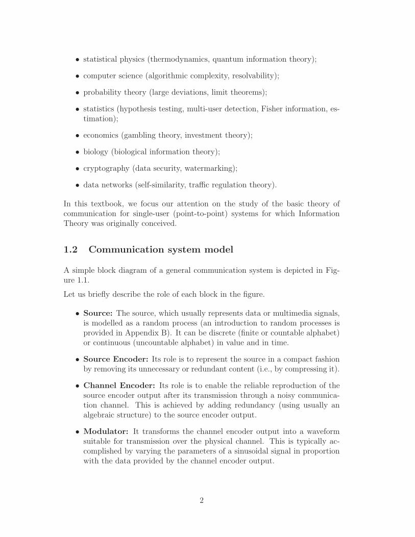
• statistical physics (thermodynamics, quantum information theory);
• computer science (algorithmic complexity, resolvability);
• probability theory (large deviations, limit theorems);
• statistics (hypothesis testing, multi-user detection, Fisher information, es-timation);
• economics (gambling theory, investment theory);
• biology (biological information theory);
• cryptography (data security, watermarking);
• data networks (self-similarity, traffic regulation theory).
In this textbook, we focus our attention on the study of the basic theory ofcommunication for single-user (point-to-point) systems for which InformationTheory was originally conceived.
1.2 Communication system model
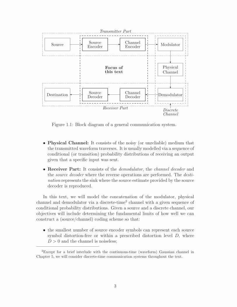
A simple block diagram of a general communication system is depicted in Fig-ure 1.1.
Let us briefly describe the role of each block in the figure.
• Source: The source, which usually represents data or multimedia signals,is modelled as a random process (an introduction to random processes isprovided in Appendix B). It can be discrete (finite or countable alphabet)or continuous (uncountable alphabet) in value and in time.
• Source Encoder: Its role is to represent the source in a compact fashionby removing its unnecessary or redundant content (i.e., by compressing it).
• Channel Encoder: Its role is to enable the reliable reproduction of thesource encoder output after its transmission through a noisy communica-tion channel. This is achieved by adding redundancy (using usually analgebraic structure) to the source encoder output.
• Modulator: It transforms the channel encoder output into a waveformsuitable for transmission over the physical channel. This is typically ac-complished by varying the parameters of a sinusoidal signal in proportionwith the data provided by the channel encoder output.
2
Source - - - Modulator
?PhysicalChannel
?
DemodulatorDestination
6DiscreteChannel
Transmitter Part
Receiver Part
Focus of
this text
SourceEncoder
ChannelEncoder
ChannelDecoder
SourceDecoder
Figure 1.1: Block diagram of a general communication system.
• Physical Channel: It consists of the noisy (or unreliable) medium thatthe transmitted waveform traverses. It is usually modelled via a sequence ofconditional (or transition) probability distributions of receiving an outputgiven that a specific input was sent.
• Receiver Part: It consists of the demodulator, the channel decoder andthe source decoder where the reverse operations are performed. The desti-nation represents the sink where the source estimate provided by the sourcedecoder is reproduced.
In this text, we will model the concatenation of the modulator, physicalchannel and demodulator via a discrete-time2 channel with a given sequence ofconditional probability distributions. Given a source and a discrete channel, ourobjectives will include determining the fundamental limits of how well we canconstruct a (source/channel) coding scheme so that:
• the smallest number of source encoder symbols can represent each sourcesymbol distortion-free or within a prescribed distortion level D, whereD > 0 and the channel is noiseless;
2Except for a brief interlude with the continuous-time (waveform) Gaussian channel inChapter 5, we will consider discrete-time communication systems throughout the text.
3
• the largest rate of information can be transmitted over a noisy channelbetween the channel encoder input and the channel decoder output withan arbitrarily small probability of decoding error;
• we can guarantee that the source is transmitted over a noisy channel andreproduced at the destination within distortion D, where D > 0.
We refer the reader to Appendix A for the necessary background on supremaand limits; in particular, Observation A.5 (resp. Observation A.11) provides apertinent connection between the supremum (resp., infimum) of a set and theproof of a typical channel coding (resp., source coding) theorem in InformationTheory. Finally, Appendix B provides an overview of basic concepts from pro-bability theory and the theory of random processes that are used in the text.The appendix also contains a brief discussion of convexity, Jensen’s inequalityand the Lagrange multipliers technique in convex optimization.
4
Chapter 2
Information Measures for DiscreteSystems
In this chapter, we define Shannon’s information measures due for discrete-timediscrete-alphabet1 systems from a probabilistic standpoint and develop theirproperties. Elucidating the operational significance of probabilistically definedinformation measures vis-a-vis the fundamental limits of coding constitutes amain objective of this book; this will be seen in the subsequent chapters.
2.1 Entropy, joint entropy and conditional entropy
2.1.1 Self-information
Let E be an event belonging to a given event space and having probabilityPr(E) , pE, where 0 ≤ pE ≤ 1. Let I(E) – called the self-information of E –represent the amount of information one gains when learning that E has occurred(or equivalently, the amount of uncertainty one had about E prior to learningthat it has happened). A natural question to ask is “what properties should I(E)have?” Although the answer to this question may vary from person to person,here are some common properties that I(E) is reasonably expected to have.
1. I(E) should be a decreasing function of pE.
In other words, this property first states that I(E) = I(pE), where I(·) isa real-valued function defined over [0, 1]. Furthermore, one would expectthat the less likely event E is, the more information is gained when one
1By discrete alphabets, one usually means finite or countably infinite alphabets. We how-ever mostly focus on finite alphabet systems, although the presented information measuresallow for countable alphabets (when they exist).
5

learns it has occurred. In other words, I(pE) is a decreasing function ofpE.
2. I(pE) should be continuous in pE.
Intuitively, one should expect that a small change in pE corresponds to asmall change in the amount of information carried by E.
3. If E1 and E2 are independent events, then I(E1 ∩ E2) = I(E1) + I(E2),or equivalently, I(pE1 × pE2) = I(pE1) + I(pE2).
This property declares that when events E1 and E2 are independent fromeach other (i.e., when they do not affect each other probabilistically), theamount of information one gains by learning that both events have jointlyoccurred should be equal to the sum of the amounts of information of eachindividual event.
Next, we show that the only function that satisfies properties 1-3 above isthe logarithmic function.
Theorem 2.1 The only function defined over p ∈ [0, 1] and satisfying
1. I(p) is monotonically decreasing in p;
2. I(p) is a continuous function of p for 0 ≤ p ≤ 1;
3. I(p1 × p2) = I(p1) + I(p2);
is I(p) = −c · logb(p), where c is a positive constant and the base b of thelogarithm is any number larger than one.
Proof:
Step 1: Claim. For n = 1, 2, 3, · · · ,
I
(1
n
)
= −c · logb
(1
n
)
,
where c > 0 is a constant.
Proof: First note that for n = 1, condition 3 directly shows the claim, sinceit yields that I(1) = I(1) + I(1). Thus I(1) = 0 = −c logb(1).
Now let n be a fixed positive integer greater than 1. Conditions 1 and 3respectively imply
n < m ⇒ I
(1
n
)
< I
(1
m
)
(2.1.1)
6
and
I
(1
mn
)
= I
(1
m
)
+ I
(1
n
)
(2.1.2)
where n,m = 1, 2, 3, · · · . Now using (2.1.2), we can show by induction (onk) that
I
(1
nk
)
= k · I(
1
n
)
(2.1.3)
for all non-negative integers k.
Now for any positive integer r, there exists a non-negative integer k suchthat
nk ≤ 2r < nk+1.
By (2.1.1), we obtain
I
(1
nk
)
≤ I
(1
2r
)
< I
(1
nk+1
)
,
which together with (2.1.3), yields
k · I(
1
n
)
≤ r · I(
1
2
)
< (k + 1) · I(
1
n
)
.
Hence, since I(1/n) > I(1) = 0,
k
r≤ I(1/2)
I(1/n)≤ k + 1
r.
On the other hand, by the monotonicity of the logarithm, we obtain
logb nk ≤ logb 2r ≤ logb nk+1 ⇔ k
r≤ logb(2)
logb(n)≤ k + 1
r.
Therefore, ∣∣∣∣
logb(2)
logb(n)− I(1/2)
I(1/n)
∣∣∣∣<
1
r.
Since n is fixed, and r can be made arbitrarily large, we can let r → ∞ toget:
I
(1
n
)
= c · logb(n).
where c = I(1/2)/ logb(2) > 0. This completes the proof of the claim.
7

Step 2: Claim. I(p) = −c · logb(p) for positive rational number p, where c > 0is a constant.
Proof: A positive rational number p can be represented by a ratio of twointegers, i.e., p = r/s, where r and s are both positive integers. Thencondition 3 yields that
I
(1
s
)
= I
(r
s
1
r
)
= I(r
s
)
+ I
(1
r
)
,
which, from Step 1, implies that
I(p) = I(r
s
)
= I
(1
s
)
− I
(1
r
)
= c · logb s − c · logb r = −c · logb p.
Step 3: For any p ∈ [0, 1], it follows by continuity and the density of the ratio-nals in the reals that
I(p) = lima↑p, a rational
I(a) = limb↓p, b rational
I(b) = −c · logb(p).
2
The constant c above is by convention normalized to c = 1. Furthermore,the base b of the logarithm determines the type of units used in measuringinformation. When b = 2, the amount of information is expressed in bits (i.e.,binary digits). When b = e – i.e., the natural logarithm (ln) is used – informationis measured in nats (i.e., natural units or digits). For example, if the event Econcerns a Heads outcome from the toss of a fair coin, then its self-informationis I(E) = − log2(1/2) = 1 bit or − ln(1/2) = 0.693 nats.
More generally, under base b > 1, information is in b-ary units or digits.For the sake of simplicity, we will throughout use the base-2 logarithm unlessotherwise specified. Note that one can easily convert information units from bitsto b-ary units by dividing the former by log2(b).
2.1.2 Entropy
Let X be a discrete random variable taking values in a finite alphabet X undera probability distribution or probability mass function (pmf) PX(x) , P [X = x]for all x ∈ X . Note that X generically represents a memoryless source, whichis a discrete-time random process Xn∞n=1 with independent and identicallydistributed (i.i.d.) random variables (cf. Appendix B).2
2We will interchangeably use the notations Xn∞n=1 and Xn to denote discrete-timerandom processes.
8
Definition 2.2 (Entropy) The entropy of a discrete random variable X withpmf PX(·) is denoted by H(X) or H(PX) and defined by
H(X) , −∑
x∈XPX(x) · log2 PX(x) (bits).
Thus H(X) represents the statistical average (mean) amount of informationone gains when learning that one of its |X | outcomes has occurred, where |X |denotes the size of alphabet X . Indeed, we directly note from the definition that
H(X) = E[− log2 PX(X)] = E[I(X)]
where I(x) , − log2 PX(x) is the self-information of the elementary event [X =x].
When computing the entropy, we adopt the convention
0 · log2 0 = 0,
which can be justified by a continuity argument since x log2 x → 0 as x → 0.Also note that H(X) only depends on the probability distribution of X and isnot affected by the symbols that represent the outcomes. For example whentossing a fair coin, we can denote Heads by 2 (instead of 1) and Tail by 100(instead of 0), and the entropy of the random variable representing the outcomewould remain equal to log2(2) = 1 bit.
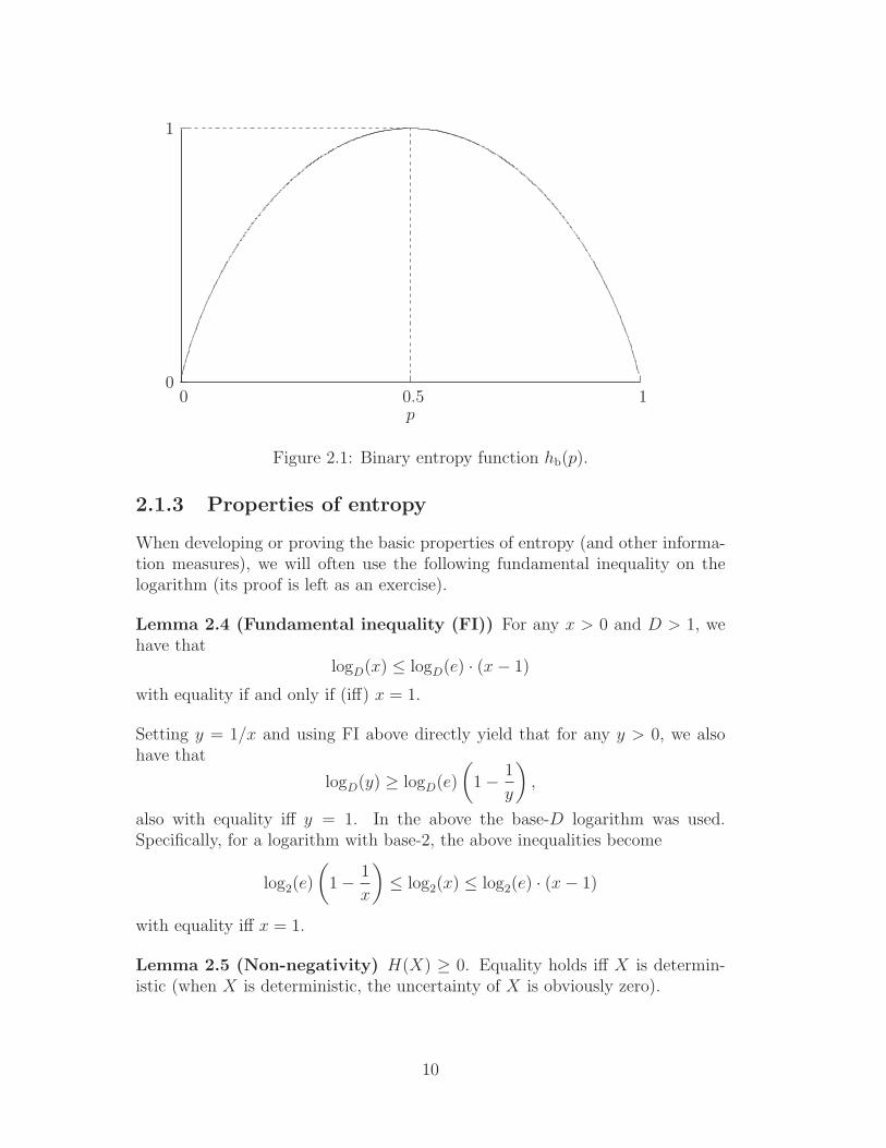
Example 2.3 Let X be a binary (valued) random variable with alphabet X =0, 1 and pmf given by PX(1) = p and PX(0) = 1− p, where 0 ≤ p ≤ 1 is fixed.Then H(X) = −p·log2 p−(1−p)·log2(1−p). This entropy is conveniently calledthe binary entropy function and is usually denoted by hb(p): it is illustrated inFigure 2.1. As shown in the figure, hb(p) is maximized for a uniform distribution(i.e., p = 1/2).
The units for H(X) above are in bits as base-2 logarithm is used. Setting
HD(X) , −∑
x∈XPX(x) · logD PX(x)
yields the entropy in D-ary units, where D > 1. Note that we abbreviate H2(X)as H(X) throughout the book since bits are common measure units for a codingsystem, and hence
HD(X) =H(X)
log2 D.
Thus
He(X) =H(X)
log2(e)= (ln 2) · H(X)
gives the entropy in nats, where e is the base of the natural logarithm.
9
0
1
0 0.5 1p
Figure 2.1: Binary entropy function hb(p).
2.1.3 Properties of entropy
When developing or proving the basic properties of entropy (and other informa-tion measures), we will often use the following fundamental inequality on thelogarithm (its proof is left as an exercise).
Lemma 2.4 (Fundamental inequality (FI)) For any x > 0 and D > 1, wehave that
logD(x) ≤ logD(e) · (x − 1)
with equality if and only if (iff) x = 1.
Setting y = 1/x and using FI above directly yield that for any y > 0, we alsohave that
logD(y) ≥ logD(e)
(
1 − 1
y
)
,
also with equality iff y = 1. In the above the base-D logarithm was used.Specifically, for a logarithm with base-2, the above inequalities become
log2(e)
(
1 − 1
x
)
≤ log2(x) ≤ log2(e) · (x − 1)
with equality iff x = 1.
Lemma 2.5 (Non-negativity) H(X) ≥ 0. Equality holds iff X is determin-istic (when X is deterministic, the uncertainty of X is obviously zero).
10

Proof: 0 ≤ PX(x) ≤ 1 implies that log2[1/PX(x)] ≥ 0 for every x ∈ X . Hence,
H(X) =∑
x∈XPX(x) log2
1
PX(x)≥ 0,
with equality holding iff PX(x) = 1 for some x ∈ X . 2
Lemma 2.6 (Upper bound on entropy) If a random variable X takes val-ues from a finite set X , then
H(X) ≤ log2 |X |,where |X | denotes the size of the set X . Equality holds iff X is equiprobable oruniformly distributed over X (i.e., PX(x) = 1
|X | for all x ∈ X ).
Proof:
log2 |X | − H(X) = log2 |X | ×[∑
x∈XPX(x)
]
−[
−∑
x∈XPX(x) log2 PX(x)
]
=∑
x∈XPX(x) × log2 |X | +
∑
x∈XPX(x) log2 PX(x)
=∑
x∈XPX(x) log2[|X | × PX(x)]
≥∑
x∈XPX(x) · log2(e)
(
1 − 1
|X | × PX(x)
)
= log2(e)∑
x∈X
(
PX(x) − 1
|X |
)
= log2(e) · (1 − 1) = 0
where the inequality follows from the FI Lemma, with equality iff (∀ x ∈ X ),|X | × PX(x) = 1, which means PX(·) is a uniform distribution on X . 2
Intuitively, H(X) tells us how random X is. Indeed, X is deterministic (notrandom at all) iff H(X) = 0. If X is uniform (equiprobable), H(X) is maximized,and is equal to log2 |X |.
Lemma 2.7 (Log-sum inequality) For non-negative numbers, a1, a2, . . ., an
and b1, b2, . . ., bn,
n∑
i=1
(
ai logD
ai
bi
)
≥(
n∑
i=1
ai
)
logD
∑ni=1 ai
∑ni=1 bi
(2.1.4)
with equality holding iff, (∀ 1 ≤ i ≤ n) (ai/bi) = (a1/b1), a constant independentof i. (By convention, 0 · logD(0) = 0, 0 · logD(0/0) = 0 and a · logD(a/0) = ∞ ifa > 0. Again, this can be justified by “continuity.”)
11

Proof: Let a ,∑n
i=1 ai and b ,∑n
i=1 bi. Then
n∑
i=1
ai logD
ai
bi
− a logD
a
b= a
n∑
i=1
ai
alogD
ai
bi
−(
n∑
i=1
ai
a
)
︸ ︷︷ ︸
=1
logD
a
b
= a
n∑
i=1
ai
alogD
[ai
bi
b
a
]
≥ a logD(e)n∑
i=1
ai
a
[
1 − bi
ai
a
b
]
= a logD(e)
(n∑
i=1
ai
a−
n∑
i=1
bi
b
)
= a logD(e) (1 − 1) = 0
where the inequality follows from the FI Lemma, with equality holing iff ai
bi
ba
= 1for all i; i.e., ai
bi= a
b∀i.
We also provide another proof using Jensen’s inequality (cf. Theorem B.17in Appendix B). Without loss of generality, assume that ai > 0 and bi > 0 forevery i. Jensen’s inequality states that
n∑
i=1
αif(ti) ≥ f
(n∑
i=1
αiti
)
for any strictly convex function f(·), αi ≥ 0, and∑n
i=1 αi = 1; equality holdsiff ti is a constant for all i. Hence by setting αi = bi/
∑nj=1 bj, ti = ai/bi, and
f(t) = t · logD(t), we obtain the desired result. 2
2.1.4 Joint entropy and conditional entropy
Given a pair of random variables (X,Y ) with a joint pmf PX,Y (·, ·) defined onX × Y ,3 the self-information of the (two-dimensional) elementary event [X =x, Y = y] is defined by
I(x, y) , − log2 PX,Y (x, y).
This leads us to the definition of joint entropy.
3Note that PXY (·, ·) is another common notation for the joint distribution PX,Y (·, ·).
12

Definition 2.8 (Joint entropy) The joint entropy H(X,Y ) of random vari-ables (X,Y ) is defined by
H(X,Y ) , −∑
(x,y)∈X×YPX,Y (x, y) · log2 PX,Y (x, y)
= E[− log2 PX,Y (X,Y )].
The conditional entropy can also be similarly defined as follows.
Definition 2.9 (Conditional entropy) Given two jointly distributed randomvariables X and Y , the conditional entropy H(Y |X) of Y given X is defined by
H(Y |X) ,∑
x∈XPX(x)
(
−∑
y∈YPY |X(y|x) · log2 PY |X(y|x)
)
(2.1.5)
where PY |X(·|·) is the conditional pmf of Y given X.
Equation (2.1.5) can be written into three different but equivalent forms:
H(Y |X) = −∑
(x,y)∈X×YPX,Y (x, y) · log2 PY |X(y|x)
= E[− log2 PY |X(Y |X)]
=∑
x∈XPX(x) · H(Y |X = x)
where H(Y |X = x) , −∑y∈Y PY |X(y|x) log2 PY |X(y|x).
The relationship between joint entropy and conditional entropy is exhibitedby the fact that the entropy of a pair of random variables is the entropy of oneplus the conditional entropy of the other.
Theorem 2.10 (Chain rule for entropy)
H(X,Y ) = H(X) + H(Y |X). (2.1.6)
Proof: SincePX,Y (x, y) = PX(x)PY |X(y|x),
we directly obtain that
H(X,Y ) = E[− log PX,Y (X,Y )]
= E[− log2 PX(X)] + E[− log2 PY |X(Y |X)]
= H(X) + H(Y |X).
13

2
By its definition, joint entropy is commutative; i.e., H(X,Y ) = H(Y,X).Hence,
H(X,Y ) = H(X) + H(Y |X) = H(Y ) + H(X|Y ) = H(Y,X),
which implies that
H(X) − H(X|Y ) = H(Y ) − H(Y |X). (2.1.7)
The above quantity is exactly equal to the mutual information which will beintroduced in the next section.
The conditional entropy can be thought of in terms of a channel whose inputis the random variable X and whose output is the random variable Y . H(X|Y ) isthen called the equivocation4 and corresponds to the uncertainty in the channelinput from the receiver’s point-of-view. For example, suppose that the set ofpossible outcomes of random vector (X,Y ) is (0, 0), (0, 1), (1, 0), (1, 1), wherenone of the elements has zero probability mass. When the receiver Y receives 1,he still cannot determine exactly what the sender X observes (it could be either1 or 0); therefore, the uncertainty, from the receiver’s view point, depends onthe probabilities PX|Y (0|1) and PX|Y (1|1).
Similarly, H(Y |X), which is called prevarication,5 is the uncertainty in thechannel output from the transmitter’s point-of-view. In other words, the senderknows exactly what he sends, but is uncertain on what the receiver will finallyobtain.
A case that is of specific interest is when H(X|Y ) = 0. By its definition,H(X|Y ) = 0 if X becomes deterministic after observing Y . In such case, theuncertainty of X after giving Y is completely zero.
The next corollary can be proved similarly to Theorem 2.10.
Corollary 2.11 (Chain rule for conditional entropy)
H(X,Y |Z) = H(X|Z) + H(Y |X,Z).
2.1.5 Properties of joint entropy and conditional entropy
Lemma 2.12 (Conditioning never increases entropy) Side information Ydecreases the uncertainty about X:
H(X|Y ) ≤ H(X)
4Equivocation is an ambiguous statement one uses deliberately in order to deceive or avoidspeaking the truth.
5Prevarication is the deliberate act of deviating from the truth (it is a synonym of “equiv-ocation”).
14
with equality holding iff X and Y are independent. In other words, “condition-ing” reduces entropy.
Proof:
H(X) − H(X|Y ) =∑
(x,y)∈X×YPX,Y (x, y) · log2
PX|Y (x|y)
PX(x)
=∑
(x,y)∈X×YPX,Y (x, y) · log2
PX|Y (x|y)PY (y)
PX(x)PY (y)
=∑
(x,y)∈X×YPX,Y (x, y) · log2
PX,Y (x, y)
PX(x)PY (y)
≥
∑
(x,y)∈X×YPX,Y (x, y)
log2
∑
(x,y)∈X×Y PX,Y (x, y)∑
(x,y)∈X×Y PX(x)PY (y)
= 0
where the inequality follows from the log-sum inequality, with equality holdingiff
PX,Y (x, y)
PX(x)PY (y)= constant ∀ (x, y) ∈ X × Y .
Since probability must sum to 1, the above constant equals 1, which is exactlythe case of X being independent of Y . 2
Lemma 2.13 Entropy is additive for independent random variables; i.e.,
H(X,Y ) = H(X) + H(Y ) for independent X and Y.
Proof: By the previous lemma, independence of X and Y implies H(Y |X) =H(Y ). Hence
H(X,Y ) = H(X) + H(Y |X) = H(X) + H(Y ).
2
Since conditioning never increases entropy, it follows that
H(X,Y ) = H(X) + H(Y |X) ≤ H(X) + H(Y ). (2.1.8)
The above lemma tells us that equality holds for (2.1.8) only when X is inde-pendent of Y .
A result similar to (2.1.8) also applies to conditional entropy.
15
Lemma 2.14 Conditional entropy is lower additive; i.e.,
H(X1, X2|Y1, Y2) ≤ H(X1|Y1) + H(X2|Y2).
Equality holds iff
PX1,X2|Y1,Y2(x1, x2|y1, y2) = PX1|Y1(x1|y1)PX2|Y2(x2|y2)
for all x1, x2, y1 and y2.
Proof: Using the chain rule for conditional entropy and the fact that condition-ing reduces entropy, we can write
H(X1, X2|Y1, Y2) = H(X1|Y1, Y2) + H(X2|X1, Y1, Y2)
≤ H(X1|Y1, Y2) + H(X2|Y1, Y2), (2.1.9)
≤ H(X1|Y1) + H(X2|Y2). (2.1.10)
For (2.1.9), equality holds iff X1 and X2 are conditionally independent given(Y1, Y2): PX1,X2|Y1,Y2(x1, x2|y1, y2) = PX1|Y1,Y2(x1|y1, y2)PX2|Y1,Y2(x2|y1, y2). For(2.1.10), equality holds iff X1 is conditionally independent of Y2 given Y1 (i.e.,PX1|Y1,Y2(x1|y1, y2) = PX1|Y1(x1|y1)), and X2 is conditionally independent of Y1
given Y2 (i.e., PX2|Y1,Y2(x2|y1, y2) = PX2|Y2(x2|y2)). Hence, the desired equalitycondition of the lemma is obtained. 2
2.2 Mutual information
For two random variables X and Y , the mutual information between X and Y isthe reduction in the uncertainty of Y due to the knowledge of X (or vice versa).A dual definition of mutual information states that it is the average amount ofinformation that Y has (or contains) about X or X has (or contains) about Y .
We can think of the mutual information between X and Y in terms of achannel whose input is X and whose output is Y . Thereby the reduction of theuncertainty is by definition the total uncertainty of X (i.e., H(X)) minus theuncertainty of X after observing Y (i.e., H(X|Y )) Mathematically, it is
mutual information = I(X; Y ) , H(X) − H(X|Y ). (2.2.1)
It can be easily verified from (2.1.7) that mutual information is symmetric; i.e.,I(X; Y ) = I(Y ; X).
16

H(X) H(X|Y ) I(X; Y ) H(Y |X) H(Y )
H(X,Y )
R
-
Figure 2.2: Relation between entropy and mutual information.
2.2.1 Properties of mutual information
Lemma 2.15
1. I(X; Y ) =∑
x∈X
∑
y∈YPX,Y (x, y) log2
PX,Y (x, y)
PX(x)PY (y).
2. I(X; Y ) = I(Y ; X).
3. I(X; Y ) = H(X) + H(Y ) − H(X,Y ).
4. I(X; Y ) ≤ H(X) with equality holding iff X is a function of Y (i.e., X =f(Y ) for some function f(·)).
5. I(X; Y ) ≥ 0 with equality holding iff X and Y are independent.
6. I(X; Y ) ≤ minlog2 |X |, log2 |Y|.
Proof: Properties 1, 2, 3, and 4 follow immediately from the definition. Property5 is a direct consequence of Lemma 2.12. Property 6 holds iff I(X; Y ) ≤ log2 |X |and I(X; Y ) ≤ log2 |Y|. To show the first inequality, we write I(X; Y ) = H(X)−H(X|Y ), use the fact that H(X|Y ) is non-negative and apply Lemma 2.6. Asimilar proof can be used to show that I(X; Y ) ≤ log2 |Y|. 2
The relationships between H(X), H(Y ), H(X,Y ), H(X|Y ), H(Y |X) andI(X; Y ) can be illustrated by the Venn diagram in Figure 2.2.
17

2.2.2 Conditional mutual information
The conditional mutual information, denoted by I(X; Y |Z), is defined as thecommon uncertainty between X and Y under the knowledge of Z. It is mathe-matically defined by
I(X; Y |Z) , H(X|Z) − H(X|Y, Z). (2.2.2)
Lemma 2.16 (Chain rule for mutual information)
I(X; Y, Z) = I(X; Y ) + I(X; Z|Y ) = I(X; Z) + I(X; Y |Z).
Proof: Without loss of generality, we only prove the first equality:
I(X; Y, Z) = H(X) − H(X|Y, Z)
= H(X) − H(X|Y ) + H(X|Y ) − H(X|Y, Z)
= I(X; Y ) + I(X; Z|Y ).
2
The above lemma can be read as: the information that (Y, Z) has about Xis equal to the information that Y has about X plus the information that Z hasabout X when Y is already known.
2.3 Properties of entropy and mutual information formultiple random variables
Theorem 2.17 (Chain rule for entropy) Let X1, X2, . . ., Xn be drawn ac-cording to PXn(xn) , PX1,··· ,Xn(x1, . . . , xn), where we use the common super-script notation to denote an n-tuple: Xn , (X1, · · · , Xn) and xn , (x1, . . . , xn).Then
H(X1, X2, . . . , Xn) =n∑
i=1
H(Xi|Xi−1, . . . , X1),
where H(Xi|Xi−1, . . . , X1) , H(X1) for i = 1. (The above chain rule can alsobe written as:
H(Xn) =n∑
i=1
H(Xi|X i−1),
where X i , (X1, . . . , Xi).)
18
Proof: From (2.1.6),
H(X1, X2, . . . , Xn) = H(X1, X2, . . . , Xn−1) + H(Xn|Xn−1, . . . , X1). (2.3.1)
Once again, applying (2.1.6) to the first term of the right-hand-side of (2.3.1),we have
H(X1, X2, . . . , Xn−1) = H(X1, X2, . . . , Xn−2) + H(Xn−1|Xn−2, . . . , X1).
The desired result can then be obtained by repeatedly applying (2.1.6). 2
Theorem 2.18 (Chain rule for conditional entropy)
H(X1, X2, . . . , Xn|Y ) =n∑
i=1
H(Xi|Xi−1, . . . , X1, Y ).
Proof: The theorem can be proved similarly to Theorem 2.17. 2
Theorem 2.19 (Chain rule for mutual information)
I(X1, X2, . . . , Xn; Y ) =n∑
i=1
I(Xi; Y |Xi−1, . . . , X1),
where I(Xi; Y |Xi−1, . . . , X1) , I(X1; Y ) for i = 1.
Proof: This can be proved by first expressing mutual information in terms ofentropy and conditional entropy, and then applying the chain rules for entropyand conditional entropy. 2
Theorem 2.20 (Independence bound on entropy)
H(X1, X2, . . . , Xn) ≤n∑
i=1
H(Xi).
Equality holds iff all the Xi’s are independent from each other.6
6This condition is equivalent to requiring that Xi be independent of (Xi−1, . . . ,X1) forall i. The equivalence can be directly proved using the chain rule for joint probabilities, i.e.,PXn(xn) =
∏ni=1 PXi|X
i−1
1
(xi|xi−11 ); it is left as an exercise.
19

Proof: By applying the chain rule for entropy,
H(X1, X2, . . . , Xn) =n∑
i=1
H(Xi|Xi−1, . . . , X1)
≤n∑
i=1
H(Xi).
Equality holds iff each conditional entropy is equal to its associated entropy, thatiff Xi is independent of (Xi−1, . . . , X1) for all i. 2
Theorem 2.21 (Bound on mutual information) If (Xi, Yi)ni=1 is a pro-
cess satisfying the conditional independence assumption PY n|Xn =∏n
i=1 PYi|Xi,
then
I(X1, . . . , Xn; Y1, . . . , Yn) ≤n∑
i=1
I(Xi; Yi)
with equality holding iff Xini=1 are independent.
Proof: From the independence bound on entropy, we have
H(Y1, . . . , Yn) ≤n∑
i=1
H(Yi).
By the conditional independence assumption, we have
H(Y1, . . . , Yn|X1, . . . , Xn) = E[− log2 PY n|Xn(Y n|Xn)
]
= E
[
−n∑
i=1
log2 PYi|Xi(Yi|Xi)
]
=n∑
i=1
H(Yi|Xi).
Hence
I(Xn; Y n) = H(Y n) − H(Y n|Xn)
≤n∑
i=1
H(Yi) −n∑
i=1
H(Yi|Xi)
=n∑
i=1
I(Xi; Yi)
with equality holding iff Yini=1 are independent, which holds iff Xin
i=1 areindependent. 2
20

Source -UEncoder -X
Channel -YDecoder -V
I(U ; V ) ≤ I(X; Y )
“By processing, we can only reduce (mutual) information,but the processed information may be in a more useful form!”
Figure 2.3: Communication context of the data processing lemma.
2.4 Data processing inequality
Lemma 2.22 (Data processing inequality) (This is also called the data pro-cessing lemma.) If X → Y → Z, then I(X; Y ) ≥ I(X; Z).
Proof: The Markov chain relationship X → Y → Z means that X and Zare conditional independent given Y (cf. Appendix B); we directly have thatI(X; Z|Y ) = 0. By the chain rule for mutual information,
I(X; Z) + I(X; Y |Z) = I(X; Y, Z) (2.4.1)
= I(X; Y ) + I(X; Z|Y )
= I(X; Y ). (2.4.2)
Since I(X; Y |Z) ≥ 0, we obtain that I(X; Y ) ≥ I(X; Z) with equality holdingiff I(X; Y |Z) = 0. 2
The data processing inequality means that the mutual information will notincrease after processing. This result is somewhat counter-intuitive since giventwo random variables X and Y , we might believe that applying a well-designedprocessing scheme to Y , which can be generally represented by a mapping g(Y ),could possibly increase the mutual information. However, for any g(·), X →Y → g(Y ) forms a Markov chain which implies that data processing cannotincrease mutual information. A communication context for the data processinglemma is depicted in Figure 2.3, and summarized in the next corollary.
Corollary 2.23 For jointly distributed random variables X and Y and anyfunction g(·), we have X → Y → g(Y ) and
I(X; Y ) ≥ I(X; g(Y )).
We also note that if Z obtains all the information about X through Y , thenknowing Z will not help increase the mutual information between X and Y ; thisis formalized in the following.
21

Corollary 2.24 If X → Y → Z, then
I(X; Y |Z) ≤ I(X; Y ).
Proof: The proof directly follows from (2.4.1) and (2.4.2). 2
It is worth pointing out that it is possible that I(X; Y |Z) > I(X; Y ) when X,Y and Z do not form a Markov chain. For example, let X and Y be independentequiprobable binary zero-one random variables, and let Z = X + Y . Then,
I(X; Y |Z) = H(X|Z) − H(X|Y, Z)
= H(X|Z)
= PZ(0)H(X|z = 0) + PZ(1)H(X|z = 1) + PZ(2)H(X|z = 2)
= 0 + 0.5 + 0
= 0.5 bits,
which is clearly larger than I(X; Y ) = 0.
Finally, we observe that we can extend the data processing inequality for asequence of random variables forming a Markov chain:
Corollary 2.25 If X1 → X2 → · · · → Xn, then for any i, j, k.l such that1 ≤ i ≤ j ≤ k ≤ l ≤ n, we have that
I(Xi; Xl) ≤ I(Xj; Xk).
2.5 Fano’s inequality
Fano’s inequality is a quite useful tool widely employed in Information Theoryto prove converse results for coding theorems (as we will see in the followingchapters).
Lemma 2.26 (Fano’s inequality) Let X and Y be two random variables, cor-related in general, with alphabets X and Y , respectively, where X is finite butY can be countably infinite. Let X , g(Y ) be an estimate of X from observingY , where g : Y → X is a given estimation function. Define the probability oferror as
Pe , Pr[X 6= X].
Then the following inequality holds
H(X|Y ) ≤ hb(Pe) + Pe · log2(|X | − 1), (2.5.1)
where hb(x) , −x log2 x− (1−x) log2(1−x) for 0 ≤ x ≤ 1 is the binary entropyfunction.
22
Observation 2.27
• Note that when Pe = 0, we obtain that H(X|Y ) = 0 (see (2.5.1)) asintuition suggests, since if Pe = 0, then X = g(Y ) = X (with probability1) and thus H(X|Y ) = H(g(Y )|Y ) = 0.
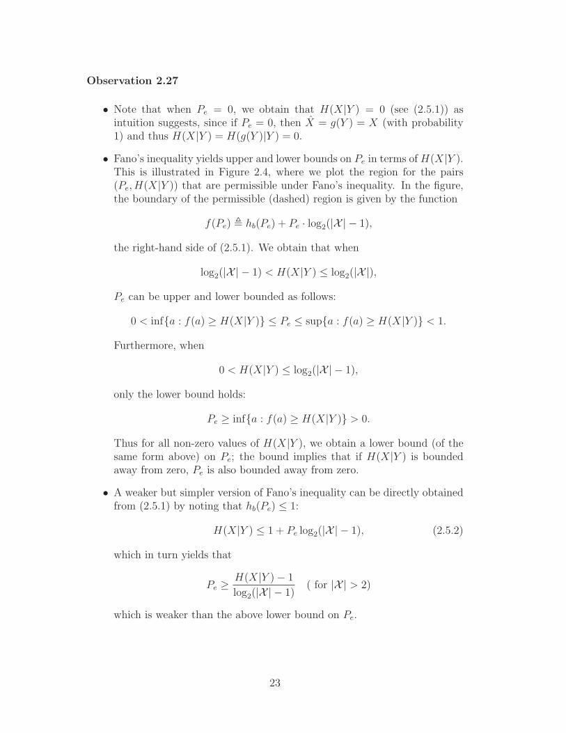
• Fano’s inequality yields upper and lower bounds on Pe in terms of H(X|Y ).This is illustrated in Figure 2.4, where we plot the region for the pairs(Pe, H(X|Y )) that are permissible under Fano’s inequality. In the figure,the boundary of the permissible (dashed) region is given by the function
f(Pe) , hb(Pe) + Pe · log2(|X | − 1),
the right-hand side of (2.5.1). We obtain that when
log2(|X | − 1) < H(X|Y ) ≤ log2(|X |),
Pe can be upper and lower bounded as follows:
0 < infa : f(a) ≥ H(X|Y ) ≤ Pe ≤ supa : f(a) ≥ H(X|Y ) < 1.
Furthermore, when
0 < H(X|Y ) ≤ log2(|X | − 1),
only the lower bound holds:
Pe ≥ infa : f(a) ≥ H(X|Y ) > 0.
Thus for all non-zero values of H(X|Y ), we obtain a lower bound (of thesame form above) on Pe; the bound implies that if H(X|Y ) is boundedaway from zero, Pe is also bounded away from zero.
• A weaker but simpler version of Fano’s inequality can be directly obtainedfrom (2.5.1) by noting that hb(Pe) ≤ 1:
H(X|Y ) ≤ 1 + Pe log2(|X | − 1), (2.5.2)
which in turn yields that
Pe ≥H(X|Y ) − 1
log2(|X | − 1)( for |X | > 2)
which is weaker than the above lower bound on Pe.
23

log2(|X | − 1)
log2(|X |)
H(X|Y )
(|X | − 1)/|X |0 1Pe
Figure 2.4: Permissible (Pe, H(X|Y )) region due to Fano’s inequality.
Proof of Lemma 2.26:
Define a new random variable,
E ,
1, if g(Y ) 6= X0, if g(Y ) = X
.
Then using the chain rule for conditional entropy, we obtain
H(E,X|Y ) = H(X|Y ) + H(E|X,Y )
= H(E|Y ) + H(X|E, Y ).
Observe that E is a function of X and Y ; hence, H(E|X,Y ) = 0. Since con-ditioning never increases entropy, H(E|Y ) ≤ H(E) = hb(Pe). The remainingterm, H(X|E, Y ), can be bounded as follows:
H(X|E, Y ) = Pr[E = 0]H(X|Y,E = 0) + Pr[E = 1]H(X|Y,E = 1)
≤ (1 − Pe) · 0 + Pe · log2(|X | − 1),
since X = g(Y ) for E = 0, and given E = 1, we can upper bound the conditionalentropy by the logarithm of the number of remaining outcomes, i.e., (|X | − 1).Combining these results completes the proof. 2
Fano’s inequality cannot be improved in the sense that the lower bound,H(X|Y ), can be achieved for some specific cases. Any bound that can be
24

achieved in some cases is often referred to as sharp.7 From the proof of the abovelemma, we can observe that equality holds in Fano’s inequality, if H(E|Y ) =H(E) and H(X|Y,E = 1) = log2(|X | − 1). The former is equivalent to E beingindependent of Y , and the latter holds iff PX|Y (·|y) is uniformly distributed overthe set X −g(y). We can therefore create an example in which equality holdsin Fano’s inequality.
Example 2.28 Suppose that X and Y are two independent random variableswhich are both uniformly distributed on the alphabet 0, 1, 2. Let the estimat-ing function be given by g(y) = y. Then
Pe = Pr[g(Y ) 6= X] = Pr[Y 6= X] = 1 −2∑
x=0
PX(x)PY (x) =2
3.
In this case, equality is achieved in Fano’s inequality, i.e.,
hb
(2
3
)
+2
3· log2(3 − 1) = H(X|Y ) = H(X) = log2 3.
To conclude this section, we present an alternative proof for Fano’s inequalityto illustrate the use of the data processing inequality and the FI Lemma.
Alternative Proof of Fano’s inequality: Noting that X → Y → X form aMarkov chain, we directly obtain via the data processing inequality that
I(X; Y ) ≥ I(X; X),
which implies thatH(X|Y ) ≤ H(X|X).
Thus, if we show that H(X|X) is no larger than the right-hand side of (2.5.1),the proof of (2.5.1) is complete.
Noting that
Pe =∑
x∈X
∑
x∈X :x6=x
PX,X(x, x)
and1 − Pe =
∑
x∈X
∑
x∈X :x=x
PX,X(x, x) =∑
x∈XPX,X(x, x),
we obtain that
H(X|X) − hb(Pe) − Pe log2(|X | − 1)
7Definition. A bound is said to be sharp if the bound is achievable for some specific cases.
A bound is said to be tight if the bound is achievable for all cases.
25
=∑
x∈X
∑
x∈X :x 6=x
PX,X(x, x) log2
1
PX|X(x|x)+∑
x∈XPX,X(x, x) log2
1
PX|X(x|x)
−[∑
x∈X
∑
x∈X :x 6=x
PX,X(x, x)
]
log2
(|X | − 1)
Pe
+
[∑
x∈XPX,X(x, x)
]
log2(1 − Pe)
=∑
x∈X
∑
x∈X :x 6=x
PX,X(x, x) log2
Pe
PX|X(x|x)(|X | − 1)
+∑
x∈XPX,X(x, x) log2
1 − Pe
PX|X(x|x)(2.5.3)
≤ log2(e)∑
x∈X
∑
x∈X :x 6=x
PX,X(x, x)
[
Pe
PX|X(x|x)(|X | − 1)− 1
]
+ log2(e)∑
x∈XPX,X(x, x)
[
1 − Pe
PX|X(x|x)− 1
]
= log2(e)
[
Pe
(|X | − 1)
∑
x∈X
∑
x∈X :x 6=x
PX(x) −∑
x∈X
∑
x∈X :x6=x
PX,X(x, x)
]
+ log2(e)
[
(1 − Pe)∑
x∈XPX(x) −
∑
x∈XPX,X(x, x)
]
= log2(e)
[Pe
(|X | − 1)(|X | − 1) − Pe
]
+ log2(e) [(1 − Pe) − (1 − Pe)]
= 0
where the inequality follows by applying the FI Lemma to each logarithm termin (2.5.3). 2
2.6 Divergence and variational distance
In addition to the probabilistically defined entropy and mutual information, an-other measure that is frequently considered in information theory is divergence orrelative entropy. In this section, we define this measure and study its statisticalproperties.
Definition 2.29 (Divergence) Given two discrete random variables X and Xdefined over a common alphabet X , the divergence (other names are Kullback-Leibler divergence or distance, relative entropy and discrimination) is denoted
26

by D(X‖X) or D(PX‖PX) and defined by8
D(X‖X) = D(PX‖PX) , EX
[
log2
PX(X)
PX(X)
]
=∑
x∈XPX(x) log2
PX(x)
PX(x).
In other words, the divergence D(PX‖PX) is the expectation (with respect toPX) of the log-likelihood ratio log2[PX/PX ] of distribution PX against distribu-
tion PX . D(X‖X) can be viewed as a measure of “distance” or “dissimilarity”
between distributions PX and PX . D(X‖X) is also called relative entropy sinceit can be regarded as a measure of the inefficiency of mistakenly assuming thatthe distribution of a source is PX when the true distribution is PX . For example,if we know the true distribution PX of a source, then we can construct a losslessdata compression code with average codeword length achieving entropy H(X)(this will be studied in the next chapter). If, however, we mistakenly thoughtthat the “true” distribution is PX and employ the “best” code corresponding toPX , then the resultant average codeword length becomes
∑
x∈X[−PX(x) · log2 PX(x)].
As a result, the relative difference between the resultant average codeword lengthand H(X) is the relative entropy D(X‖X). Hence, divergence is a measure ofthe system cost (e.g., storage consumed) paid due to mis-classifying the systemstatistics.
Note that when computing divergence, we follow the convention that
0 · log2
0
p= 0 and p · log2
p
0= ∞ for p > 0.
We next present some properties of the divergence and discuss its relation withentropy and mutual information.
Lemma 2.30 (Non-negativity of divergence)
D(X‖X) ≥ 0
with equality iff PX(x) = PX(x) for all x ∈ X (i.e., the two distributions areequal).
8In order to be consistent with the units (in bits) adopted for entropy and mutual informa-tion, we will also use the base-2 logarithm for divergence unless otherwise specified.
27
Proof:
D(X‖X) =∑
x∈XPX(x) log2
PX(x)
PX(x)
≥(∑
x∈XPX(x)
)
log2
∑
x∈X PX(x)∑
x∈X PX(x)
= 0
where the second step follows from the log-sum inequality with equality holdingiff for every x ∈ X ,
PX(x)
PX(x)=
∑
a∈X PX(a)∑
b∈X PX(b),
or equivalently PX(x) = PX(x) for all x ∈ X . 2
Lemma 2.31 (Mutual information and divergence)
I(X; Y ) = D(PX,Y ‖PX × PY ),
where PX,Y (·, ·) is the joint distribution of the random variables X and Y andPX(·) and PY (·) are the respective marginals.
Proof: The observation follows directly from the definitions of divergence andmutual information. 2
Definition 2.32 (Refinement of distribution) Given distribution PX on X ,divide X into k mutually disjoint sets, U1,U2, . . . ,Uk, satisfying
X =k⋃
i=1
Ui.
Define a new distribution PU on U = 1, 2, · · · , k as
PU(i) =∑
x∈Ui
PX(x).
Then PX is called a refinement (or more specifically, a k-refinement) of PU .
Let us briefly discuss the relation between the processing of information andits refinement. Processing of information can be modeled as a (many-to-one)mapping, and refinement is actually the reverse operation. Recall that thedata processing lemma shows that mutual information can never increase due
28

to processing. Hence, if one wishes to increase mutual information, he shouldsimultaneously “anti-process” (or refine) the involved statistics.
From Lemma 2.31, the mutual information can be viewed as the divergenceof a joint distribution against the product distribution of the marginals. It istherefore reasonable to expect that a similar effect due to processing (or a reverseeffect due to refinement) should also apply to divergence. This is shown in thenext lemma.
Lemma 2.33 (Refinement cannot decrease divergence) Let PX and PX
be the refinements (k-refinements) of PU and PU respectively. Then
D(PX‖PX) ≥ D(PU‖PU).
Proof: By the log-sum inequality, we obtain that for any i ∈ 1, 2, · · · , k
∑
x∈Ui
PX(x) log2
PX(x)
PX(x)≥
(∑
x∈Ui
PX(x)
)
log2
∑
x∈UiPX(x)
∑
x∈UiPX(x)
= PU(i) log2
PU(i)
PU(i), (2.6.1)
with equality iffPX(x)
PX(x)=
PU(i)
PU(i)
for all x ∈ U . Hence,
D(PX‖PX) =k∑
i=1
∑
x∈Ui
PX(x) log2
PX(x)
PX(x)
≥k∑
i=1
PU(i) log2
PU(i)
PU(i)
= D(PU‖PU),
with equality iff
(∀ i)(∀ x ∈ Ui)PX(x)
PX(x)=
PU(i)
PU(i).
2
Observation 2.34 One drawback of adopting the divergence as a measure be-tween two distributions is that it does not meet the symmetry requirement of a
29

true distance,9 since interchanging its two arguments may yield different quan-tities. In other words, D(PX‖PX) 6= D(PX‖PX) in general. (It also does notsatisfy the triangular inequality.) Thus divergence is not a true distance or met-ric. Another measure which is a true distance, called variational distance, issometimes used instead.
Definition 2.35 (Variational distance) The variational distance (or L1-distance)between two distributions PX and PX with common alphabet X is defined by
‖PX − PX‖ ,∑
x∈X|PX(x) − PX(x)|.
Lemma 2.36 The variational distance satisfies
‖PX − PX‖ = 2 · supE⊂X
|PX(E) − PX(E)| = 2 ·∑
x∈X :PX(x)>PX(x)
[PX(x) − PX(x)] .
Proof: We first show that ‖PX − PX‖ = 2 ·∑x∈X :PX(x)>PX(x) [PX(x) − PX(x)] .
Setting A , x ∈ X : PX(x) > PX(x), we have
‖PX − PX‖ =∑
x∈X|PX(x) − PX(x)|
=∑
x∈A|PX(x) − PX(x)| +
∑
x∈Ac
|PX(x) − PX(x)|
=∑
x∈A[PX(x) − PX(x)] +
∑
x∈Ac
[PX(x) − PX(x)]
=∑
x∈A[PX(x) − PX(x)] + PX (Ac) − PX (Ac)
=∑
x∈A[PX(x) − PX(x)] + PX(A) − PX(A)
=∑
x∈A[PX(x) − PX(x)] +
∑
x∈A[PX(x) − PX(x)]
9Given a non-empty set A, the function d : A × A → [0,∞) is called a distance or metricif it satisfies the following properties.
1. Non-negativity: d(a, b) ≥ 0 for every a, b ∈ A with equality holding iff a = b.
2. Symmetry: d(a, b) = d(b, a) for every a, b ∈ A.
3. Triangular inequality: d(a, b) + d(b, c) ≥ d(a, c) for every a, b, c ∈ A.
30

= 2 ·∑
x∈A[PX(x) − PX(x)]
where Ac denotes the complement set of A.
We next prove that ‖PX − PX‖ = 2 · supE⊂X |PX(E) − PX(E)| by showingthat each quantity is greater than or equal to the other. For any set E ⊂ X , wecan write
‖PX − PX‖ =∑
x∈X|PX(x) − PX(x)|
=∑
x∈E
|PX(x) − PX(x)| +∑
x∈Ec
|PX(x) − PX(x)|
≥∣∣∣∣∣
∑
x∈E
[PX(x) − PX(x)]
∣∣∣∣∣+
∣∣∣∣∣
∑
x∈Ec
[PX(x) − PX(x)]
∣∣∣∣∣
= |PX(E) − PX(E)| + |PX(Ec) − PX(Ec)|= |PX(E) − PX(E)| + |PX(E) − PX(E)|= 2 · |PX(E) − PX(E)|.
Thus ‖PX − PX‖ ≥ 2 · supE⊂X |PX(E) − PX(E)|. Conversely, we have that
2 · supE⊂X
|PX(E) − PX(E)| ≥ 2 · |PX(A) − PX(A)|
= |PX(A) − PX(A)| + |PX(Ac) − PX(Ac)|
=
∣∣∣∣∣
∑
x∈A[PX(x) − PX(x)]
∣∣∣∣∣+
∣∣∣∣∣
∑
x∈Ac
[PX(x) − PX(x)]
∣∣∣∣∣
=∑
x∈A|PX(x) − PX(x)| +
∑
x∈Ac
|PX(x) − PX(x)|
= ‖PX − PX‖.
Therefore, ‖PX − PX‖ = 2 · supE⊂X |PX(E) − PX(E)| . 2
Lemma 2.37 (Variational distance vs divergence: Pinsker’s inequality)
D(X‖X) ≥ log2(e)
2· ‖PX − PX‖2.
This result is referred to as Pinsker’s inequality.
Proof:
1. With A , x ∈ X : PX(x) > PX(x), we have from the previous lemmathat
‖PX − PX‖ = 2[PX(A) − PX(A)].
31

2. Define two random variables U and U as:
U =
1, if X ∈ A;0, if X ∈ Ac,
and
U =
1, if X ∈ A;
0, if X ∈ Ac.
Then PX and PX are refinements (2-refinements) of PU and PU , respec-tively. From Lemma 2.33, we obtain that
D(PX‖PX) ≥ D(PU‖PU).
3. The proof is complete if we show that
D(PU‖PU) ≥ 2 log2(e)[PX(A) − PX(A)]2
= 2 log2(e)[PU(1) − PU(1)]2.
For ease of notations, let p = PU(1) and q = PU(1). Then to prove theabove inequality is equivalent to show that
p · ln p
q+ (1 − p) · ln 1 − p
1 − q≥ 2(p − q)2.
Define
f(p, q) , p · ln p
q+ (1 − p) · ln 1 − p
1 − q− 2(p − q)2,
and observe that
df(p, q)
dq= (p − q)
(
4 − 1
q(1 − q)
)
≤ 0 for q ≤ p.
Thus, f(p, q) is non-increasing in q for q ≤ p. Also note that f(p, q) = 0for q = p. Therefore,
f(p, q) ≥ 0 for q ≤ p.
The proof is completed by noting that
f(p, q) ≥ 0 for q ≥ p,
since f(1 − p, 1 − q) = f(p, q).
2
32

Observation 2.38 The above lemma tells us that for a sequence of distributions(PXn , PXn
)n≥1, when D(PXn‖PXn) goes to zero as n goes to infinity, ‖PXn −
PXn‖ goes to zero as well. But the converse does not necessarily hold. For a
quick counterexample, let
PXn(0) = 1 − PXn(1) = 1/n > 0
andPXn
(0) = 1 − PXn(1) = 0.
In this case,D(PXn‖PXn
) → ∞since by convention, (1/n) · log2((1/n)/0) → ∞. However,
‖PX − PX‖ = 2
[
PX
(x : PX(x) > PX(x)
)− PX
(x : PX(x) > PX(x)
)]
=2
n→ 0.
We however can upper bound D(PX‖PX) by the variational distance betweenPX and PX when D(PX‖PX) < ∞.
Lemma 2.39 If D(PX‖PX) < ∞, then
D(PX‖PX) ≤ log2(e)
minx : PX(x)>0
minPX(x), PX(x) · ‖PX − PX‖.
Proof: Without loss of generality, we assume that PX(x) > 0 for all x ∈ X .Since D(PX‖PX) < ∞, we have that for any x ∈ X , PX(x) > 0 implies thatPX(x) > 0. Let
t , minx∈X : PX(x)>0
minPX(x), PX(x).
Then for all x ∈ X ,
lnPX(x)
PX(x)≤
∣∣∣∣ln
PX(x)
PX(x)
∣∣∣∣
≤∣∣∣∣
maxminPX(x),PX(x)≤s≤maxPX(x),PX(x)
d ln(s)
ds
∣∣∣∣· |PX(x) − PX(x)|
=1
minPX(x), PX(x) · |PX(x) − PX(x)|
≤ 1
t· |PX(x) − PX(x)|.
33

Hence,
D(PX‖PX) = log2(e)∑
x∈XPX(x) · ln PX(x)
PX(x)
≤ log2(e)
t
∑
x∈XPX(x) · |PX(x) − PX(x)|
≤ log2(e)
t
∑
x∈X|PX(x) − PX(x)|
=log2(e)
t· ‖PX − PX‖.
2
The next lemma discusses the effect of side information on divergence. Asstated in Lemma 2.12, side information usually reduces entropy; it, however,increases divergence. One interpretation of these results is that side informationis useful. Regarding entropy, side information provides us more information, souncertainty decreases. As for divergence, it is the measure or index of how easyone can differentiate the source from two candidate distributions. The largerthe divergence, the easier one can tell apart between these two distributionsand make the right guess. At an extreme case, when divergence is zero, onecan never tell which distribution is the right one, since both produce the samesource. So, when we obtain more information (side information), we should beable to make a better decision on the source statistics, which implies that thedivergence should be larger.
Definition 2.40 (Conditional divergence) Given three discrete random vari-ables, X, X and Z, where X and X have a common alphabet X , we define theconditional divergence between X and X given Z by
D(X‖X|Z) = D(PX|Z‖PX|Z) ,∑
z∈Z
∑
x∈XPX,Z(x, z) log
PX|Z(x|z)
PX|Z(x|z).
In other words, it is the expected value with respect to PX,Z of the log-likelihood
ratio logPX|Z
PX|Z. Note that another notation encountered in the literature for the
above conditional divergence is D(PX|Z‖PX|Z |PZ) as we can write
∑
z∈Z
∑
x∈XPX,Z(x, z) log
PX|Z(x|z)
PX|Z(x|z)=∑
z∈ZPZ(z)
∑
x∈XPX|Z(x|z) log
PX|Z(x|z)
PX|Z(x|z).
Lemma 2.41 (Conditional mutual information and conditional diver-gence) Given three discrete random variables X, Y and Z with alphabets X ,
34

Y and Z, respectively, and joint distribution PX,Y,Z , then
I(X; Y |Z) = D(PX,Y |Z‖PX|ZPY |Z)
=∑
x∈X
∑
y∈Y
∑
z∈ZPX,Y,Z(x, y, z) log2
PX,Y |Z(x, y|z)
PX|Z(x|z)PY |Z(y|z),
where PX,Y |Z is conditional joint distribution of X and Y given Z, and PX|Z andPY |Z are the conditional distributions of X and Y , respectively, given Z.
Proof: The proof follows directly from the definition of conditional mutual in-formation (2.2.2) and the above definition of conditional divergence. 2
Lemma 2.42 (Chain rule for divergence) Let PXn and QXn be two jointdistributions on X n. We have that
D(PX1,X2‖QX1,X2) = D(PX1‖QX1) + D(PX2|X1‖QX2|X1),
and more generally,
D(PXn‖QXn) =n∑
i=1
D(PXi|Xi−1‖QXi|Xi−1),
where D(PXi|Xi−1‖QXi|Xi−1) , D(PX1‖QX1) for i = 1.
Proof: The proof readily follows from the divergence definitions. 2
Lemma 2.43 (Conditioning never decreases divergence) For three discreterandom variables, X, X and Z, where X and X have a common alphabet X ,we have that
D(PX|Z‖PX|Z) ≥ D(PX‖PX).
Proof:
D(PX|Z‖PX|Z) − D(PX‖PX)
=∑
z∈Z
∑
x∈XPX,Z(x, z) · log2
PX|Z(x|z)
PX|Z(x|z)−∑
x∈XPX(x) · log2
PX(x)
PX(x)
=∑
z∈Z
∑
x∈XPX,Z(x, z) · log2
PX|Z(x|z)
PX|Z(x|z)−∑
x∈X
(∑
z∈ZPX,Z(x, z)
)
· log2
PX(x)
PX(x)
=∑
z∈Z
∑
x∈XPX,Z(x, z) · log2
PX|Z(x|z)PX(x)
PX|Z(x|z)PX(x)
35

≥∑
z∈Z
∑
x∈XPX,Z(x, z) · log2(e)
(
1 −PX|Z(x|z)PX(x)
PX|Z(x|z)PX(x)
)
(by the FI Lemma)
= log2(e)
(
1 −∑
x∈X
PX(x)
PX(x)
∑
z∈ZPZ(z)PX|Z(x|z)
)
= log2(e)
(
1 −∑
x∈X
PX(x)
PX(x)PX(x)
)
= log2(e)
(
1 −∑
x∈XPX(x)
)
= 0
with equality holding iff for all x and z,
PX(x)
PX(x)=
PX|Z(x|z)
PX|Z(x|z).
2
Note that it is not necessary that
D(PX|Z‖PX|Z) ≥ D(PX‖PX).
In other words, the side information is helpful for divergence only when it pro-vides information on the similarity or difference of the two distributions. For theabove case, Z only provides information about X, and Z provides informationabout X; so the divergence certainly cannot be expected to increase. The nextlemma shows that if (Z, Z) are independent of (X, X), then the side informationof (Z, Z) does not help in improving the divergence of X against X.
Lemma 2.44 (Independent side information does not change diver-gence) If (X, X) is independent of (Z, Z), then
D(PX|Z‖PX|Z) = D(PX‖PX),
where
D(PX|Z‖PX|Z) ,∑
x∈X
∑
z∈ZPX,Z(x, z) log2
PX|Z(x|z)
PX|Z(x|z).
Proof: This can be easily justified by the definition of divergence. 2
Lemma 2.45 (Additivity of divergence under independence)
D(PX,Z‖PX,Z) = D(PX‖PX) + D(PZ‖PZ),
provided that (X, X) is independent of (Z, Z).
Proof: This can be easily proved from the definition. 2
36

2.7 Convexity/concavity of information measures
We next address the convexity/concavity properties of information measureswith respect to the distributions on which they are defined. Such properties willbe useful when optimizing the information measures over distribution spaces.
Lemma 2.46
1. H(PX) is a concave function of PX , namely
H(λPX + (1 − λ)P eX) ≥ λH(PX) + (1 − λ)H(P eX).
2. Noting that I(X; Y ) can be re-written as I(PX , PY |X), where
I(PX , PY |X) ,∑
x∈X
∑
y∈YPY |X(y|x)PX(x) log2
PY |X(y|x)∑
a∈X PY |X(y|a)PX(a),
then I(X; Y ) is a concave function of PX (for fixed PY |X), and a convexfunction of PY |X (for fixed PX).
3. D(PX‖PX) is convex with respect to both the first argument PX and thesecond argument PX . It is also convex in the pair (PX , PX); i.e., if (PX , PX)and (QX , QX) are two pairs of probability mass functions, then
D(λPX + (1 − λ)QX‖λPX + (1 − λ)QX)
≤ λ · D(PX‖PX) + (1 − λ) · D(QX‖QX), (2.7.1)
for all λ ∈ [0, 1].
Proof:
1. The proof uses the log-sum inequality:
H(λPX + (1 − λ)P eX) −[λH(PX) + (1 − λ)H(P eX)
]
= λ∑
x∈XPX(x) log2
PX(x)
λPX(x) + (1 − λ)P eX(x)
+(1 − λ)∑
x∈XP eX(x) log2
P eX(x)
λPX(x) + (1 − λ)P eX(x)
≥ λ
(∑
x∈XPX(x)
)
log2
∑
x∈X PX(x)∑
x∈X [λPX(x) + (1 − λ)P eX(x)]
37

+(1 − λ)
(∑
x∈XP eX(x)
)
log2
∑
x∈X P eX(x)∑
x∈X [λPX(x) + (1 − λ)P eX(x)]
= 0,
with equality holding iff PX(x) = P eX(x) for all x.
2. We first show the concavity of I(PX , PY |X) with respect to PX . Let λ =1 − λ.
I(λPX + λP eX , PY |X) − λI(PX , PY |X) − λI(P eX , PY |X)
= λ∑
y∈Y
∑
x∈XPX(x)PY |X(y|x) log2
∑
x∈XPX(x)PY |X(y|x)
∑
x∈X[λPX(x) + λP eX(x)]PY |X(y|x)]
+ λ∑
y∈Y
∑
x∈XP eX(x)PY |X(y|x) log2
∑
x∈XP eX(x)PY |X(y|x)
∑
x∈X[λPX(x) + λP eX(x)]PY |X(y|x)]
≥ 0 (by the log-sum inequality)
with equality holding iff∑
x∈XPX(x)PY |X(y|x) =
∑
x∈XP eX(x)PY |X(y|x)
for all y ∈ Y . We now turn to the convexity of I(PX , PY |X) with respect to
PY |X . For ease of notation, let PYλ(y) , λPY (y)+λPeY (y), and PYλ|X(y|x) ,
λPY |X(y|x) + λPeY |X(y|x). Then
λI(PX , PY |X) + λI(PX , PeY |X) − I(PX , λPY |X + λPeY |X)
= λ∑
x∈X
∑
y∈YPX(x)PY |X(y|x) log2
PY |X(y|x)
PY (y)
+λ∑
x∈X
∑
y∈YPX(x)PeY |X(y|x) log2
PeY |X(y|x)
PeY (y)
−∑
x∈X
∑
y∈YPX(x)PYλ|X(y|x) log2
PYλ|X(y|x)
PYλ(y)
= λ∑
x∈X
∑
y∈YPX(x)PY |X(y|x) log2
PY |X(y|x)PYλ(y)
PY (y)PYλ|X(y|x)
+λ∑
x∈X
∑
y∈YPX(x)PeY |X(y|x) log2
PeY |X(y|x)PYλ(y)
PeY (y)PYλ|X(y|x)
38
≥ λ log2(e)∑
x∈X
∑
y∈YPX(x)PY |X(y|x)
(
1 − PY (y)PYλ|X(y|x)
PY |X(y|x)PYλ(y)
)
+λ log2(e)∑
x∈X
∑
y∈YPX(x)PeY |X(y|x)
(
1 − PeY (y)PYλ|X(y|x)
PeY |X(y|x)PYλ(y)
)
= 0,
where the inequality follows from the FI Lemma, with equality holding iff
(∀ x ∈ X , y ∈ Y)PY (y)
PY |X(y|x)=
PeY (y)
PeY |X(y|x).
3. For ease of notation, let PXλ(x) , λPX(x) + (1 − λ)P eX(x).
λD(PX‖PX) + (1 − λ)D(P eX‖PX) − D(PXλ‖PX)
= λ∑
x∈XPX(x) log2
PX(x)
PXλ(x)
+ (1 − λ)∑
x∈XP eX(x) log2
P eX(x)
PXλ(x)
= λD(PX‖PXλ) + (1 − λ)D(P eX‖PXλ
)
≥ 0
by the non-negativity of the divergence, with equality holding iff PX(x) =P eX(x) for all x.
Similarly, by letting PXλ(x) , λPX(x) + (1 − λ)P eX(x), we obtain:
λD(PX‖PX) + (1 − λ)D(PX‖P eX) − D(PX‖PXλ)
= λ∑
x∈XPX(x) log2
PXλ(x)
PX(x)+ (1 − λ)
∑
x∈XPX(x) log2
PXλ(x)
P eX(x)
≥ λ
ln 2
∑
x∈XPX(x)
(
1 − PX(x)
PXλ(x)
)
+(1 − λ)
ln 2
∑
x∈XPX(x)
(
1 − P eX(x)
PXλ(x)
)
= log2(e)
(
1 −∑
x∈XPX(x)
λPX(x) + (1 − λ)P eX(x)
PXλ(x)
)
= 0,
where the inequality follows from the FI Lemma, with equality holding iffP eX(x) = PX(x) for all x.
Finally, by the log-sum inequality, for each x ∈ X , we have
(λPX(x) + (1 − λ)QX(x)) log2
λPX(x) + (1 − λ)QX(x)
λPX(x) + (1 − λ)QX(x)
39

≤ λPX(x) log2
λPX(x)
λPX(x)+ (1 − λ)QX(x) log2
(1 − λ)QX(x)
(1 − λ)QX(x).
Summing over x, we yield (2.7.1).
Note that the last result (convexity of D(PX‖PX) in the pair (PX , PX))actually implies the first two results: just set PX = QX to show convexityin the first argument PX , and set PX = QX to show convexity in the secondargument PX .
2
2.8 Fundamentals of hypothesis testing
One of the fundamental problems in statistics is to decide between two alternativeexplanations for the observed data. For example, when gambling, one may wishto test whether it is a fair game or not. Similarly, a sequence of observations onthe market may reveal the information that whether a new product is successfulor not. This is the simplest form of the hypothesis testing problem, which isusually named simple hypothesis testing.
It has quite a few applications in information theory. One of the frequentlycited examples is the alternative interpretation of the law of large numbers.Another example is the computation of the true coding error (for universal codes)by testing the empirical distribution against the true distribution. All of thesecases will be discussed subsequently.
The simple hypothesis testing problem can be formulated as follows:
Problem: Let X1, . . . , Xn be a sequence of observations which is possibly dr-awn according to either a “null hypothesis” distribution PXn or an “alternativehypothesis” distribution PXn . The hypotheses are usually denoted by:
• H0 : PXn
• H1 : PXn
Based on one sequence of observations xn, one has to decide which of the hy-potheses is true. This is denoted by a decision mapping φ(·), where
φ(xn) =
0, if distribution of Xn is classified to be PXn ;1, if distribution of Xn is classified to be PXn .
Accordingly, the possible observed sequences are divided into two groups:
Acceptance region for H0 : xn ∈ X n : φ(xn) = 0
40

Acceptance region for H1 : xn ∈ X n : φ(xn) = 1.
Hence, depending on the true distribution, there are possibly two types of pro-bability of errors:
Type I error : αn = αn(φ) , PXn (xn ∈ X n : φ(xn) = 1)Type II error : βn = βn(φ) , PXn (xn ∈ X n : φ(xn) = 0) .
The choice of the decision mapping is dependent on the optimization criterion.Two of the most frequently used ones in information theory are:
1. Bayesian hypothesis testing.
Here, φ(·) is chosen so that the Bayesian cost
π0αn + π1βn
is minimized, where π0 and π1 are the prior probabilities for the nulland alternative hypotheses, respectively. The mathematical expression forBayesian testing is:
minφ
[π0αn(φ) + π1βn(φ)] .
2. Neyman Pearson hypothesis testing subject to a fixed test level.
Here, φ(·) is chosen so that the type II error βn is minimized subject to aconstant bound on the type I error; i.e.,
αn ≤ ε
where ε > 0 is fixed. The mathematical expression for Neyman-Pearsontesting is:
minφ : αn(φ)≤ε
βn(φ).
The set φ considered in the minimization operation could have two differentranges: range over deterministic rules, and range over randomization rules. Themain difference between a randomization rule and a deterministic rule is that theformer allows the mapping φ(xn) to be random on 0, 1 for some xn, while thelatter only accept deterministic assignments to 0, 1 for all xn. For example, arandomization rule for specific observations xn can be
φ(xn) = 0, with probability 0.2;
φ(xn) = 1, with probability 0.8.
The Neyman-Pearson lemma shows the well-known fact that the likelihoodratio test is always the optimal test.
41

Lemma 2.47 (Neyman-Pearson Lemma) For a simple hypothesis testingproblem, define an acceptance region for the null hypothesis through the likeli-hood ratio as
An(τ) ,
xn ∈ X n :PXn(xn)
PXn(xn)> τ
,
and letα∗
n , PXn Acn(τ)
andβ∗
n , PXn An(τ) .
Then for type I error αn and type II error βn associated with another choice ofacceptance region for the null hypothesis, we have
αn ≤ α∗n ⇒ βn ≥ β∗
n.
Proof: Let B be a choice of acceptance region for the null hypothesis. Then
αn + τβn =∑
xn∈Bc
PXn(xn) + τ∑
xn∈BPXn(xn)
=∑
xn∈Bc
PXn(xn) + τ
[
1 −∑
xn∈Bc
PXn(xn)
]
= τ +∑
xn∈Bc
[PXn(xn) − τPXn(xn)] . (2.8.1)
Observe that (2.8.1) is minimized by choosing B = An(τ). Hence,
αn + τβn ≥ α∗n + τβ∗
n,
which immediately implies the desired result. 2
The Neyman-Pearson lemma indicates that no other choices of acceptance re-gions can simultaneously improve both type I and type II errors of the likelihoodratio test. Indeed, from (2.8.1), it is clear that for any αn and βn, one can alwaysfind a likelihood ratio test that performs as good. Therefore, the likelihood ratiotest is an optimal test. The statistical properties of the likelihood ratio thusbecome essential in hypothesis testing. Note that, when the observations arei.i.d. under both hypotheses, the divergence, which is the statistical expectationof the log-likelihood ratio, plays an important role in hypothesis testing (fornon-memoryless observations, one is then concerned with the divergence rate, anextended notion of divergence for systems with memory which will be defined ina following chapter).
42

2.9 Renyi’s information measures
We close this chapter by briefly introducing generalized information measuresdue to Renyi [228] which subsume Shannon’s measures as a limiting case.
Definition 2.48 (Renyi’s entropy) Given a parameter α > 0 with α 6= 1,and given a discrete random variable X with alphabet X and distribution PX ,then its Renyi entropy of order α is given by
Hα(X) =1
1 − αlog
(∑
x∈XPX(x)α
)
. (2.9.1)
As in case of the Shannon entropy, the base of the logarithm determines theunits; if the base is D, Renyi’s entropy is in D-ary units. Other notations forHα(X) are H(X; α), Hα(PX) and H(PX ; α).
Definition 2.49 (Renyi’s divergence) Given a parameter 0 < α < 1, andtwo discrete random variables X and X with common alphabet X and distribu-tion PX and PX , respectively, then the Renyi divergence of order α between X
and X is given by
Dα(X‖X) =1
α − 1log
(∑
x∈X
[
PαX(x)P 1−α
X(x)])
. (2.9.2)
This definition can be extended to α > 1 if PX(x) > 0 for all x ∈ X . Other
notations for Dα(X‖X) are D(X‖X; α), Dα(PX‖PX) and D(PX‖PX ; α).
As in the case of Shannon’s information measures, the base of the logarithmindicates the units of the measure and can be changed from 2 to an arbitraryb > 1. In the next lemma, whose proof is left as an exercise, we note that inthe limit of α tending to 1, Shannon’s entropy and divergence can be recoveredfrom Renyi’s entropy and divergence, respectively.
Lemma 2.50 When α → 1, we have the following:
limα→1
Hα(X) = H(X) (2.9.3)
andlimα→1
Dα(X‖X) = D(X‖X). (2.9.4)
43

Observation 2.51 (Operational meaning of Renyi’s information mea-sures) Renyi’s entropy has been shown to have an operational chracterization formany problems, including lossless variable-length source coding under an expo-nential cost constraint [44, 37, 45, 221] (see also Observation 3.29 in Chapter 3),buffer overflow in source coding [150], fixed-length source coding [60, 52] andothers areas [229, 1, 23, 15, 219]. Furthermore, Renyi’s divergence has played aprominent role in hypothesis testing questions [157, 136, 197, 198, 60, 12].
Observation 2.52 (α-mutual information) While Renyi did not propose amutual information of order α that generalizes Shannon’s mutual information,there are at least three different possible definitions of such measure due toSibson [251], Arimoto [18] and Csiszar [60], respectively. We refer the readerto [60] and [279] for discussions on the properties and merits of these differentmeasures.
Observation 2.53 (Information measures for continuous distributions)Note that the above information measures defined for discrete distributions cansimilarly be defined for continuous distributions admitting densities with theusual straightforward modifications (with densities replacing pmf’s and inte-grals replacing summations). See Chapter 5 for a study of Shannon’s differentialentropy and divergence for continuous distributions (also for continuous distri-butions, closed-form expressions for Shannon’s differential entropy and Renyi’sentropy can be found in [260] and expressions for Renyi’s divergence are derivedin [177, 106].)
Problems
1. Prove the FI Lemma.
2. Show that the two conditions in Footnote 6 are equivalent.
3. For a finite-alphabet random variable X, show that H(X) ≤ log2 |X | usingthe log-sum inequality.
4. Given a pair of random variables (X,Y ), is H(X|Y ) = H(Y |X)? Whendo we have equality?
5. Given a random variable X, what is the relationship between H(X) andH(Y ) when Y is defined as follows.
(a) Y = log2(X)?
(b) Y = sin(X)?
44
6. Show that the entropy of a real-valued function f of X is less than or equalto the entropy of X?
Hint: By the chain rule for entropy,
H(X, f(X)) = H(X) + H(f(X)|X) = H(f(X)) + H(X|f(X)).
7. Show that H(Y |X) = 0 iff Y is a function of X.
8. Give examples of:
(a) I(X; Y |Z) < I(X; Y ).
(b) I(X; Y |Z) > I(X; Y ).
Hint: For (a), create example for I(X; Y |Z) = 0 and I(X; Y ) > 0. For(b), create example for I(X; Y ) = 0 and I(X; Y |Z) > 0.
9. Let the joint distribution of X and Y be:
YX
0 1
01
40
11
2
1
4
Draw the Venn diagram for
H(X), H(Y ), H(X|Y ), H(Y |X), H(X,Y ) and I(X; Y ),
and indicate the quantities (in bits) for each area of the Venn diagram.
10. Maximal discrete entropy. Prove that, of all probability mass functions fora non-negative integer-valued random variable with mean µ, the geometricdistribution, given by
PZ(z) =1
1 + µ
(µ
1 + µ
)z
, for z = 0, 1, 2, . . . ,
has the largest entropy.
Hint: Let X be a non-negative integer-valued random variable with meanµ. Show that H(X)−H(Z) = −D(PX‖PZ) ≤ 0 with equality iff PX = PZ .
11. Inequalities: Which of the following inequalities are ≥, =, ≤ ? Label eachwith ≥, =, or ≤ and justify your answer.
45

(a) H(X|Z) − H(X|Y ) versus I(X; Y |Z).
(b) H(X|g(Y )) versus H(X|Y ) for a real function g.
(c) H(X1000|X999) versus limn→∞(1/n)H(Xn, Xn−1, · · · , X1) for a station-ary first-order Markov source Xn∞n=1.
12. Entropy of a sum [57]: Given random variables X and Y with finite al-phabets, define a new random variable Z as Z = X + Y .
(a) Prove that H(Z|X) = H(Y |X).
(b) Show that H(Z) ≥ H(X) and H(Z) ≥ H(Y ).
(c) Give an example such that H(X) > H(Z) and H(Y ) > H(Z).
Hint: You may create an example with H(Z) = 0, but H(X) > 0and H(Y ) > 0.
(d) Under what condition does H(Z) = H(X) + H(Y )?
13. Let X1 → X2 → X3 → · · · → Xn form a Markov chain. Show that:
(a) I(X1; X2, . . . , Xn) = I(X1; X2).
(b) For any n, H(X1|Xn−1) ≤ H(X1|Xn).
14. Prove that refinement cannot decrease H(X). Namely, given a randomvariable X with distribution PX and a partition (U1, . . . ,Um) on its alpha-bet X such that PU(i) = PX(Ui) for 1 ≤ i ≤ m, show that
H(X) ≥ H(U).
15. Provide examples for the following inequalities.
(a) D(PX|Z‖PX|Z) > D(PX ||PX).
(b) D(PX|Z‖PX|Z) < D(PX ||PX).
16. Prove that the binary divergence defined by
D(p‖q) , p log2
p
q+ (1 − p) log2
1 − p
1 − q
satisfies
D(p‖q) ≤ log2(e)(p − q)2
q(1 − q)
for 0 < p < 1 and 0 < q < 1.
Hint: Use the FI Lemma.
46
17. Let p1, p2, . . . , pm be a set of positive real numbers with∑m
i=1 pi = 1. Ifq1, q2, . . . , qm is any other set of positive real numbers with
∑mi=1 qi = α,
where α > 0 is a constant, show that
m∑
i=1
pi log1
pi
≤m∑
i=1
pi log1
qi
+ log α.
Give a necessary and sufficient condition for equality.
18. An alternative form for mutual information: Given jointly distributedrandom variables X and Y with alphabets X and Y , respectively, andwith joint distribution PX,Y = PY |XPX , show that the mutual informationI(X; Y ) can be written as
I(X; Y ) = D(PY |X‖PY |PX)
= D(PY |X‖QY |PX) − D(PY ‖QY )
for any distribution QY on Y , where PY is the marginal distribution ofPX,Y on Y and
D(PY |X‖QY |PX) =∑
x∈XPX(x)
∑
y∈YPY |X(y|x) log
PY |X(y|x)
QY (y)
is the conditional divergence between PY |X and QY given PX ; see Defini-tion 2.40.
19. Let X and Y be jointly distributed discrete random variables. Show that
I(X; Y ) ≥ I(f(X); g(Y )),
where f(·) and g(·) are given functions.
20. Data processing inequality for the divergence: Given a conditional distri-bution PY |X defined on the alphabets X and Y , let PX and QX be twodistributions on X and let PY and QY be two corresponding distributionson Y defined by
PY (y) =∑
x∈XPY |X(y|x)PX(x)
andQY (y) =
∑
x∈XPY |X(y|x)QX(x)
for all y ∈ Y . Show that
D(PX‖QX) ≥ D(PY ‖QY ).
47

21. An application of Jensen’s inequality [57]: Let X be a discrete randomvariable with distribution PX .
(a) Use Jensen’s inequality to show that
2E[log2 PX(X)] ≤ E[PX(X)].
(b) Let X ′ be another random variable that is independent of X but hasthe same distribution as X. Show that
Pr[X = X ′] ≥ 2−H(X)
with equality iff X is uniformly distributed.
(c) Now assume that X ′ has a different distribution than X (but is stillindependent of X). Show that
Pr[X = X ′] ≥ 2−H(X)−D(X‖X′).
22. Useful inequalities [132, 97]:
(a) Given a positive integer m, let Pi and Qi be positive real numbersdefined for i = 1, 2, · · · ,m, such that
m∑
i=1
Pi =m∑
i=1
Qi = 1.
Let the parameter λ satisfy 0 < λ < 1. Show that
m∑
i=1
Qλi P 1−λ
i ≤ 1,
and give a necessary and sufficient condition for equality.
(b) Holder’s inequality: Given a positive integer m, let ai and bi be pos-itive real numbers defined for i = 1, 2, · · · ,m and let parameter λsatisfy 0 < λ < 1. Show that
m∑
i=1
aibi ≤[
m∑
i=1
a1λi
]λ [ m∑
i=1
b1
1−λ
i
]1−λ
,
with equality iff for some constant c,
a1λi = cb
11−λ
i
for all i. Note that when λ = 1/2, the inequality is nothing but theso-called Cauchy-Schwarz inequality.
48
(c) Variant of Holder’s inequality: Using the same quantities in (b), showthat
m∑
i=1
Piaibi ≤[
m∑
i=1
Pia1λi
]λ [ m∑
i=1
Pib1
1−λ
i
]1−λ
,
with equality iff for some constant c,
Pia1λi = cPib
11−λ
i
for all i, where Pi is defined in (a).
23. Inequality of arithmetic and geometric means:
(a) Show thatn∑
i=1
ai ln xi ≤ ln
[n∑
i=1
aixi
]
,
where x1, x2, · · · , xn are arbitrary positive numbers, and a1, a2, · · · , an
are positive numbers such that∑n
i=1 ai = 1.
(b) Deduce from the above the inequality of the arithmetic and geometricmeans:
xa11 xa2
2 · · ·xann ≤
n∑
i=1
aixi.
24. Consider two distributions P (·) and Q(·) on the alphabet X = a1, · · · , aKsuch that Q(ai) > 0 for all i = 1, · · · , K. Show that
K∑
i=1
P (ai)2
Q(ai)≥ 1.
25. Let X be a discrete random variable with alphabet X and distribution PX .Let f : X → R be a real-valued function, and let α be an arbitrary realnumber.
(a) Show that
H(X) ≤ αE[f(X))] + log2
[∑
x∈X2−αf(x)
]
,
with equality iff PX(x) = 1A2−αf(x) for x ∈ X , where A ,
∑
x∈X 2−αf(x).
49
(b) Show that for a positive integer-valued random variable N (such thatE[N ] > 1 without loss of generality), the following holds:
H(N) ≤ log2(E[N ]) + log2 e.
Hint: First use part (a) with f(N) = N and α = log2E[N ]
E[N ]−1.
26. Fano’s inequality for list decoding: Let X and Y be two random variableswith alphabets X and Y , respectively, where X is finite and Y can becountably many. Given a fixed integer m ≥ 1, define
Xm , (g1(Y ), g2(Y ), · · · , gm(Y ))
as the list of estimates of X obtained by observing Y , where gi : Y → X isa given estimation function for i = 1, 2, · · · ,m. Define the probability oflist decoding error as
P (m)e , Pr
[
X1 6= X, X2 6= X, · · · , Xm 6= X]
.
(a) Show that
H(X|Y ) ≤ hb(P(m)e )+P (m)
e log2(|X |−u)+(1−P (m)e ) log2 (u) , (2.9.5)
whereu ,
∑
x∈X
∑
xm∈Xm : xi=x for some i
PXm(xm).
Note: When m = 1, we obtain that u = 1 and the right-hand side of(2.9.5) reduces to the original Fano inequality (cf. the right-hand sideof (2.5.1)).
Hint: Show that H(X|Y ) ≤ H(X|Xm) and that H(X|Xm) is lessthan the right-hand-side of the above inequality.
(b) Use (2.9.5) to deduce the following weaker version of Fano’s inequalityfor list decoding (see [4], [155], [224, Appendix 3.E]):
H(X|Y ) ≤ hb(P(m)e ) + P (m)
e log2 |X | + (1 − P (m)e ) log2 m. (2.9.6)
27. Fano’s inequality for ternary partitioning of the observation space: In Pr-oblem 26, P
(m)e and u can actually be expressed as
P (m)e =
∑
x∈X
∑
xm 6∈ Ux
PX,Xm(x, xm) =∑
x∈X
∑
y 6∈Yx
PX,Y (x, y)
andu =
∑
x∈X
∑
xm∈Ux
PXm(xm) =∑
x∈X
∑
y∈Yx
PY (y),
50

respectively, where
Ux , xm ∈ Xm : xi = x for some iand
Yx , y ∈ Y : gi(y) = x for some i .
Thus, given x ∈ X , Yx and Ycx form a binary partition on the observation
space Y .
Now consider again random variables X and Y with alphabets X and Y ,respectively, where X is finite and Y can be countably many, and assumethat for each x ∈ X , we are given a ternary partition Sx, Tx,Vx on theobservation space Y , where the sets Sx, Tx and Vx are mutually disjointand their union equals Y . Define
p ,∑
x∈X
∑
y∈Sx
PX,Y (x, y), q ,∑
x∈X
∑
y∈Tx
PX,Y (x, y), r ,∑
x∈X
∑
y∈Vx
PX,Y (x, y)
and
s ,∑
x∈X
∑
y∈Sx
PY (y), t ,∑
x∈X
∑
y∈Tx
PY (y), v ,∑
x∈X
∑
y∈Vx
PY (y).
Note that p + q + r = 1 and s + t + v = |X |. Show that
H(X|Y ) ≤ H(p, q, r) + p log2(s) + q log2(t) + r log2(v), (2.9.7)
where
H(p, q, r) = p log2
1
p+ q log2
1
q+ r log2
1
r.
Note: When Vx = ∅ for all x ∈ X , we obtain that Sx = T cx for all x,
r = v = 0 and p = 1 − q; as a result, inequality (2.9.7) acquires a similarexpression as (2.9.5) with p standing for the probability of error.
28. ǫ-Independence: Let X and Y be two jointly distributed random variableswith finite respective alphabets X and Y and joint pmf PX,Y defined on theX ×Y . Given a fixed ǫ > 0, random variable Y is said to be ǫ-independentfrom random variable X if
∑
x∈XPX(x)
∑
y∈Y|PY |X(y|x) − PY (y)| < ǫ
where PX and PY are the marginal pmf’s of X and Y , respectively, andPY |X is the conditional pmf of Y given X. Show that
I(X; Y ) <log2(e)
2ǫ2
is a sufficient condition for Y to be ǫ-independent from X, where I(X; Y )is the mutual information (in bits) between X and Y .
51
29. Renyi’s entropy: Given a fixed positive integer n > 1, consider an n-aryvalued random variable X with alphabet X = 1, 2, · · · , n and distri-bution described by the probabilities pi , Pr[X = i], where pi > 0 foreach i = 1, · · · , n. Given α > 0 and α 6= 1, the Renyi entropy of X (seeDefinition 2.9.1) is given by
Hα(X) ,1
1 − αlog2
[n∑
i=1
pαi
]
.
(a) Show thatn∑
i=1
pri > 1 if r < 1,
and thatn∑
i=1
pri < 1 if r > 1.
Hint: Show that the function f(r) =∑n
i=1 pri is decreasing in r, where
r > 0.
(b) Show that0 ≤ Hα(X) ≤ log2 n.
Hint: Use (a) for the lower bound, and use Jensen’s inequality (with
the convex function f(y) = y1
1−α , for y > 0) for the upper bound.
30. Renyi’s entropy and divergence: Consider two discrete random variables Xand X with common alphabet X and distribution PX and PX , respectively.
(a) Prove Lemma 2.50.
(b) Find a distribution Q on X in terms of α and PX such that thefollowing holds
Hα(X) = H(X) +1
1 − αD(PX ||Q).
52
Chapter 3
Lossless Data Compression
3.1 Principles of data compression
As mentioned in Chapter 1, data compression describes methods of representinga source by a code whose average codeword length (or code rate) is acceptablysmall. The representation can be: lossless (or asymptotically lossless) wherethe reconstructed source is identical (or asymptotically identical) to the originalsource; or lossy where the reconstructed source is allowed to deviate from theoriginal source, usually within an acceptable threshold. We herein focus onlossless data compression.
Since a memoryless source is modeled as a random variable, the averagedcodeword length of a codebook is calculated based on the probability distributionof that random variable. For example, a ternary memoryless source X exhibitsthree possible outcomes with
PX(x = outcomeA) = 0.5;
PX(x = outcomeB) = 0.25;
PX(x = outcomeC) = 0.25.
Suppose that a binary code book is designed for this source, in which outcomeA,outcomeB and outcomeC are respectively encoded as 0, 10, and 11. Then theaverage codeword length (in bits/source outcome) is
length(0) × PX(outcomeA) + length(10) × PX(outcomeB)
+length(11) × PX(outcomeC)
= 1 × 0.5 + 2 × 0.25 + 2 × 0.25
= 1.5 bits.
There are usually no constraints on the basic structure of a code. In thecase where the codeword length for each source outcome can be different, the
53

code is called a variable-length code. When the codeword lengths of all sourceoutcomes are equal, the code is referred to as a fixed-length code . It is obviousthat the minimum average codeword length among all variable-length codes isno greater than that among all fixed-length codes, since the latter is a subclass ofthe former. We will see in this chapter that the smallest achievable average coderate for variable-length and fixed-length codes coincide for sources with goodprobabilistic characteristics, such as stationarity and ergodicity. But for moregeneral sources with memory, the two quantities are different (e.g., see [128]).
For fixed-length codes, the sequence of adjacent codewords are concate-nated together for storage or transmission purposes, and some punctuationmechanism—such as marking the beginning of each codeword or delineatinginternal sub-blocks for synchronization between encoder and decoder—is nor-mally considered an implicit part of the codewords. Due to constraints on spaceor processing capability, the sequence of source symbols may be too long for theencoder to deal with all at once; therefore, segmentation before encoding is oftennecessary. For example, suppose that we need to encode using a binary code thegrades of a class with 100 students. There are three grade levels: A, B and C.By observing that there are 3100 possible grade combinations for 100 students,a straightforward code design requires ⌈log2(3
100)⌉ = 159 bits to encode thesecombinations. Now suppose that the encoder facility can only process 16 bitsat a time. Then the above code design becomes infeasible and segmentation isunavoidable. Under such constraint, we may encode grades of 10 students at atime, which requires ⌈log2(3
10)⌉ = 16 bits. As a consequence, for a class of 100students, the code requires 160 bits in total.
In the above example, the letters in the grade set A,B,C and the lettersfrom the code alphabet 0, 1 are often called source symbols and code symbols,respectively. When the code alphabet is binary (as in the previous two examples),the code symbols are referred to as code bits or simply bits (as already used).A tuple (or grouped sequence) of source symbols is called a sourceword and theresulting encoded tuple consisting of code symbols is called a codeword. (In theabove example, each sourceword consists of 10 source symbols (students) andeach codeword consists of 16 bits.)
Note that, during the encoding process, the sourceword lengths do not have tobe equal. In this text, we however only consider the case where the sourcewordshave a fixed length throughout the encoding process (except for the Lempel-Zivcode briefly discussed at the end of this chapter), but we will allow the codewordsto have fixed or variable lengths as defined earlier.1 The block diagram of a source
1In other words, our fixed-length codes are actually “fixed-to-fixed length codes” and ourvariable-length codes are “fixed-to-variable length codes” since, in both cases, a fixed numberof source symbols is mapped onto codewords with fixed and variable lengths, respectively.
54
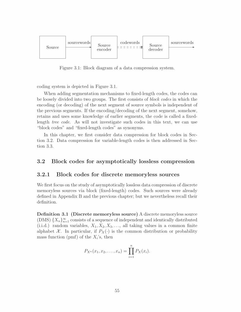
Source -sourcewords
Sourceencoder
--codewords
Sourcedecoder
-sourcewords
Figure 3.1: Block diagram of a data compression system.
coding system is depicted in Figure 3.1.
When adding segmentation mechanisms to fixed-length codes, the codes canbe loosely divided into two groups. The first consists of block codes in which theencoding (or decoding) of the next segment of source symbols is independent ofthe previous segments. If the encoding/decoding of the next segment, somehow,retains and uses some knowledge of earlier segments, the code is called a fixed-length tree code. As will not investigate such codes in this text, we can use“block codes” and “fixed-length codes” as synonyms.
In this chapter, we first consider data compression for block codes in Sec-tion 3.2. Data compression for variable-length codes is then addressed in Sec-tion 3.3.
3.2 Block codes for asymptotically lossless compression
3.2.1 Block codes for discrete memoryless sources
We first focus on the study of asymptotically lossless data compression of discretememoryless sources via block (fixed-length) codes. Such sources were alreadydefined in Appendix B and the previous chapter; but we nevertheless recall theirdefinition.
Definition 3.1 (Discrete memoryless source) A discrete memoryless source(DMS) Xn∞n=1 consists of a sequence of independent and identically distributed(i.i.d.) random variables, X1, X2, X3, . . ., all taking values in a common finitealphabet X . In particular, if PX(·) is the common distribution or probabilitymass function (pmf) of the Xi’s, then
PXn(x1, x2, . . . , xn) =n∏
i=1
PX(xi).
55

Definition 3.2 An (n,M) block code of blocklength n and size M (which canbe a function of n in general,2 i.e., M = Mn) for a discrete source Xn∞n=1 is a setc1, c2, . . . , cM ⊆ X n consisting of M reproduction (or reconstruction) words,where each reproduction word is a sourceword (an n-tuple of source symbols).3
The block code’s operation can be symbolically represented as4
(x1, x2, . . . , xn) → cm ∈ c1, c2, . . . , cM.
This procedure will be repeated for each consecutive block of length n, i.e.,
· · · (x3n, . . . , x31)(x2n, . . . , x21)(x1n, . . . , x11) → · · · |cm3 |cm2 |cm1 ,
where “|” reflects the necessity of “punctuation mechanism” or ”synchronizationmechanism” for consecutive source block coders.
The next theorem provides a key tool for proving Shannon’s source codingtheorem.
2In the literature, both (n,M) and (M,n) have been used to denote a block code withblocklength n and size M . For example, [294, p. 149] adopts the former one, while [57, p. 193]uses the latter. We use the (n,M) notation since M = Mn is a function of n in general.
3One can binary-index the reproduction words in c1, c2, . . . , cM using k , ⌈log2 M⌉ bits.As such k-bit words in 0, 1k are usually stored for retrieval at a later date, the (n,M) blockcode can be represented by an encoder-decoder pair of functions (f, g), where the encodingfunction f : Xn → 0, 1k maps each sourceword xn to a k-bit word f(xn) which we call acodeword. Then the decoding function g : 0, 1k → c1, c2, . . . , cM is a retrieving operationthat produces the reproduction words. Since the codewords are binary-valued, such a blockcode is called a binary code. More generally, a D-ary block code (where D > 1 is an integer)would use an encoding function f : Xn → 0, 1, · · · ,D − 1k where each codeword f(xn)contains k D-ary code symbols.
Furthermore, since the behavior of block codes is investigated for sufficiently large n andM (tending to infinity), it is legitimate to replace ⌈log2 M⌉ by log2 M for the case of binarycodes. With this convention, the data compression rate or code rate is
bits required per source symbol =k
n=
1
nlog2 M.
Similarly, for D-ary codes, the rate is
D-ary code symbols required per source symbol =k
n=
1
nlogD M.
For computational convenience, nats (under the natural logarithm) can be used instead ofbits or D-ary code symbols; in this case, the code rate becomes:
nats required per source symbol =1
nlog M.
4When one uses an encoder-decoder pair (f, g) to describe the block code, the code’s oper-ation can be expressed as: cm = g(f(xn)).
56
Theorem 3.3 (Shannon-McMillan) (Asymptotic equipartition propertyor AEP5) If Xn∞n=1 is a DMS with entropy H(X), then
− 1
nlog2 PXn(X1, . . . , Xn) → H(X) in probability.
In other words, for any δ > 0,
limn→∞
Pr
∣∣∣∣− 1
nlog2 PXn(X1, . . . , Xn) − H(X)
∣∣∣∣> δ
= 0.
Proof: This theorem follows by first observing that for an i.i.d. sequence Xn∞n=1,
− 1
nlog2 PXn(X1, . . . , Xn) =
1
n
n∑
i=1
[− log2 PX(Xi)]
and that the sequence − log2 PX(Xi)∞i=1 is i.i.d., and then applying the weaklaw of large numbers (WLLN) on the later sequence. 2
The AEP indeed constitutes an “information theoretic” analog of WLLN asit states that if − log2 PX(Xi)∞i=1 is an i.i.d. sequence, then for any δ > 0,
Pr
∣∣∣∣∣
1
n
n∑
i=1
[− log2 PX(Xi)] − H(X)
∣∣∣∣∣≤ δ
→ 1 as n → ∞.
As a consequence of the AEP, all the probability mass will be ultimately placedon the weakly δ-typical set, which is defined as
Fn(δ) ,
xn ∈ X n :
∣∣∣∣− 1
nlog2 PXn(xn) − H(X)
∣∣∣∣≤ δ
=
xn ∈ X n :
∣∣∣∣∣− 1
n
n∑
i=1
log2 PX(xi) − H(X)
∣∣∣∣∣≤ δ
.
Note that since the source is memoryless, for any xn ∈ Fn(δ), −(1/n) log2 PXn(xn),the normalized self-information of xn, is equal to (1/n)
∑ni=1 [− log2 PX(xi)],
which is the empirical (arithmetic) average self-information or “apparent” en-tropy of the source. Thus, a sourceword xn is δ-typical if it yields an apparentsource entropy within δ of the “true” source entropy H(X). Note that the source-words in Fn(δ) are nearly equiprobable or equally surprising (cf. Property 1 ofTheorem 3.4); this justifies naming Theorem 3.3 by AEP.
Theorem 3.4 (Consequence of the AEP) Given a DMS Xn∞n=1 with en-tropy H(X) and any δ greater than zero, then the weakly δ-typical set Fn(δ)satisfies the following.
5This is also called the entropy stability property.
57

1. If xn ∈ Fn(δ), then
2−n(H(X)+δ) ≤ PXn(xn) ≤ 2−n(H(X)−δ).
2. PXn (F cn(δ)) < δ for sufficiently large n, where the superscript “c” denotes
the complementary set operation.
3. |Fn(δ)| > (1−δ)2n(H(X)−δ) for sufficiently large n, and |Fn(δ)| ≤ 2n(H(X)+δ)
for every n, where |Fn(δ)| denotes the number of elements in Fn(δ).
Note: The above theorem also holds if we define the typical set using the base-D logarithm logD for any D > 1 instead of the base-2 logarithm; in this case,one just needs to appropriately change the base of the exponential terms in theabove theorem (by replacing 2x terms with Dx terms) and also substitute H(X)with HD(X)).
Proof: Property 1 is an immediate consequence of the definition of Fn(δ).Property 2 is a direct consequence of the AEP, since the AEP states that for afixed δ > 0, limn→∞ PXn(Fn(δ)) = 1; i.e., ∀ε > 0, there exists n0 = n0(ε) suchthat for all n ≥ n0,
PXn(Fn(δ)) > 1 − ε.
In particular, setting ε = δ yields the result. We nevertheless provide a directproof of Property 2 as we give an explicit expression for n0: observe that byChebyshev’s inequality,6
PXn(F cn(δ)) = PXn
xn ∈ X n :
∣∣∣∣− 1
nlog2 PXn(xn) − H(X)
∣∣∣∣> δ
≤ σ2X
nδ2< δ,
for n > σ2X/δ3, where the variance
σ2X , Var[− log2 PX(X)] =
∑
x∈XPX(x) [log2 PX(x)]2 − (H(X))2
is a constant7 independent of n.
6The detail for Chebyshev’s inequality as well as its proof can be found on p. 280 inAppendix B.
7In the proof, we assume that the variance σ2X = Var[− log2 PX(X)] < ∞. This holds since
the source alphabet is finite:
Var[− log2 PX(X)] ≤ E[(log2 PX(X))2] =∑
x∈X
PX(x)(log2 PX(x))2
≤∑
x∈X
4
e2[log2(e)]
2 =4
e2[log2(e)]
2 × |X | < ∞.
58
To prove Property 3, we have from Property 1 that
1 ≥∑
xn∈Fn(δ)
PXn(xn) ≥∑
xn∈Fn(δ)
2−n(H(X)+δ) = |Fn(δ)|2−n(H(X)+δ),
and, using Properties 2 and 1, we have that
1 − δ < 1 − σ2X
nδ2≤
∑
xn∈Fn(δ)
PXn(xn) ≤∑
xn∈Fn(δ)
2−n(H(X)−δ) = |Fn(δ)|2−n(H(X)−δ),
for n ≥ σ2X/δ3. 2
Note that for any n > 0, a block code C∼n = (n,M) is said to be uniquelydecodable or completely lossless if its set of reproduction words is trivially equalto the set of all source n-tuples: c1, c2, . . . , cM = X n. In this case, if we arebinary-indexing the reproduction words using an encoding-decoding pair (f, g),every sourceword xn will be assigned to a distinct binary codeword f(xn) oflength k = log2 M and all the binary k-tuples are the image under f of somesourceword. In other words, f is a bijective (injective and surjective) map andhence invertible with the decoding map g = f−1 and M = |X |n = 2k. Thus thecode rate is (1/n) log2 M = log2 |X | bits/source symbol.
Now the question becomes: can we achieve a better (i.e., smaller) compres-sion rate? The answer is affirmative: we can achieve a compression rate equal tothe source entropy H(X) (in bits), which can be significantly smaller than log2 Mwhen this source is strongly non-uniformly distributed, if we give up unique de-codability (for every n) and allow n to be sufficiently large to asymptoticallyachieve lossless reconstruction by having an arbitrarily small (but positive) pro-bability of decoding error Pe( C∼n) , PXnxn ∈ X n : g(f(xn)) 6= xn.
Thus, block codes herein can perform data compression that is asymptoticallylossless with respect to blocklength; this contrasts with variable-length codeswhich can be completely lossless (uniquely decodable) for every finite block-length.
We now can formally state and prove Shannon’s asymptotically lossless sourcecoding theorem for block codes. The theorem will be stated for general D-ary block codes, representing the source entropy HD(X) in D-ary code sym-bol/source symbol as the smallest (infimum) possible compression rate for asymp-totically lossless D-ary block codes. Without loss of generality, the theoremwill be proved for the case of D = 2. The idea behind the proof of the for-ward (achievability) part is basically to binary-index the source sequence in theweakly δ-typical set Fn(δ) to a binary codeword (starting from index one withcorresponding k-tuple codeword 0 · · · 01); and to encode all sourcewords outsideFn(δ) to a default all-zero binary codeword, which certainly cannot be repro-duced distortionless due to its many-to-one-mapping property. The resultant
59

Source
∣∣∣∣∣−1
2
2∑
i=1
log2 PX(xi) − H(X)
∣∣∣∣∣
codewordreconstructed
source sequence
AA 0.525 bits 6∈ F2(0.4) 000 ambiguousAB 0.317 bits ∈ F2(0.4) 001 ABAC 0.025 bits ∈ F2(0.4) 010 ACAD 0.475 bits 6∈ F2(0.4) 000 ambiguousBA 0.317 bits ∈ F2(0.4) 011 BABB 0.109 bits ∈ F2(0.4) 100 BBBC 0.183 bits ∈ F2(0.4) 101 BCBD 0.683 bits 6∈ F2(0.4) 000 ambiguousCA 0.025 bits ∈ F2(0.4) 110 CACB 0.183 bits ∈ F2(0.4) 111 CBCC 0.475 bits 6∈ F2(0.4) 000 ambiguousCD 0.975 bits 6∈ F2(0.4) 000 ambiguousDA 0.475 bits 6∈ F2(0.4) 000 ambiguousDB 0.683 bits 6∈ F2(0.4) 000 ambiguousDC 0.975 bits 6∈ F2(0.4) 000 ambiguousDD 1.475 bits 6∈ F2(0.4) 000 ambiguous
Table 3.1: An example of the δ-typical set with n = 2 and δ = 0.4,where F2(0.4) = AB, AC, BA, BB, BC, CA, CB . The codewordset is 001(AB), 010(AC), 011(BA), 100(BB), 101(BC), 110(CA),111(CB), 000(AA, AD, BD, CC, CD, DA, DB, DC, DD) , wherethe parenthesis following each binary codeword indicates those source-words that are encoded to this codeword. The source distribution isPX(A) = 0.4, PX(B) = 0.3, PX(C) = 0.2 and PX(D) = 0.1.
code rate is (1/n)⌈log2(|Fn(δ)| + 1)⌉ bits per source symbol. As revealed in theShannon-McMillan AEP theorem and its Consequence, almost all the probabi-lity mass will be on Fn(δ) as n sufficiently large, and hence, the probability ofnon-reconstructable source sequences can be made arbitrarily small. A simpleexample for the above coding scheme is illustrated in Table 3.1. The conversepart of the proof will establish (by expressing the probability of correct decodingin terms of the δ-typical set and also using the Consequence of the AEP) thatfor any sequence of D-ary codes with rate strictly below the source entropy, theirprobability of error cannot asymptotically vanish (is bounded away from zero).Actually a stronger result is proven: it is shown that their probability of errornot only does not asymptotically vanish, it actually ultimately grows to 1 (thisis why we call this part a “strong” converse).
60

Theorem 3.5 (Shannon’s source coding theorem) Given integer D > 1,consider a discrete memoryless source Xn∞n=1 with entropy HD(X). Then thefollowing hold.
• Forward part (achievability): For any 0 < ε < 1, there exists 0 < δ < εand a sequence of D-ary block codes C∼n = (n,Mn)∞n=1 with
lim supn→∞
1
nlogD Mn ≤ HD(X) + δ (3.2.1)
satisfyingPe( C∼n) < ε (3.2.2)
for all sufficiently large n, where Pe( C∼n) denotes the probability of decodingerror for block code C∼n.8
• Strong converse part: For any 0 < ε < 1, any sequence of D-ary blockcodes C∼n = (n,Mn)∞n=1 with
lim supn→∞
1
nlogD Mn < HD(X) (3.2.3)
satisfiesPe( C∼n) > 1 − ε
for all n sufficiently large.
Proof:
Forward Part: Without loss of generality, we will prove the result for the caseof binary codes (i.e., D = 2). Also recall that subscript D in HD(X) will bedropped (i.e., omitted) specifically when D = 2.
Given 0 < ε < 1, fix δ such that 0 < δ < ε and choose n > 2/δ. Nowconstruct a binary C∼n block code by simply mapping the δ/2-typical sourcewordsxn onto distinct not all-zero binary codewords of length k , ⌈log2 Mn⌉ bits. Inother words, binary-index (cf. the footnote in Definition 3.2) the sourcewords inFn(δ/2) with the following encoding map:
xn → binary index of xn, if xn ∈ Fn(δ/2);xn → all-zero codeword, if xn 6∈ Fn(δ/2).
8(3.2.2) is equivalent to lim supn→∞ Pe( C∼n) ≤ ε. Since ε can be made arbitrarily small,the forward part actually indicates the existence of a sequence of D-ary block codes C∼n∞n=1
satisfying (3.2.1) such that lim supn→∞ Pe( C∼n) = 0.Based on this, the converse should be that any sequence of D-ary block codes satisfying
(3.2.3) satisfies lim supn→∞ Pe( C∼n) > 0. However, the so-called strong converse actually givesa stronger consequence: lim supn→∞ Pe( C∼n) = 1 (as ǫ can be made arbitrarily small).
61

Then by the Shannon-McMillan AEP theorem, we obtain that
Mn = |Fn(δ/2)| + 1 ≤ 2n(H(X)+δ/2) + 1 < 2 · 2n(H(X)+δ/2) < 2n(H(X)+δ),
for n > 2/δ. Hence, a sequence of C∼n = (n,Mn) block code satisfying (3.2.1) isestablished. It remains to show that the error probability for this sequence of(n,Mn) block code can be made smaller than ε for all sufficiently large n.
By the Shannon-McMillan AEP theorem,
PXn(F cn(δ/2)) <
δ
2for all sufficiently large n.
Consequently, for those n satisfying the above inequality, and being bigger than2/δ,
Pe( C∼n) ≤ PXn(F cn(δ/2)) < δ ≤ ε.
(For the last step, the readers can refer to Table 3.1 to confirm that only the“ambiguous” sequences outside the typical set contribute to the probability oferror.)
Strong Converse Part: Fix any sequence of block codes C∼n∞n=1 with
lim supn→∞
1
nlog2 | C∼n| < H(X).
Let Sn be the set of source symbols that can be correctly decoded through C∼n-coding system. (A quick example is depicted in Figure 3.2.) Then |Sn| = | C∼n|.By choosing δ small enough with ε/2 > δ > 0, and also by definition of limsupoperation, we have
(∃ N0)(∀ n > N0)1
nlog2 |Sn| =
1
nlog2 | C∼n| < H(X) − 2δ,
which implies|Sn| < 2n(H(X)−2δ).
Furthermore, from Property 2 of the Consequence of the AEP, we obtain that
(∃ N1)(∀ n > N1) PXn(F cn(δ)) < δ.
Consequently, for n > N , maxN0, N1, log2(2/ε)/δ, the probability of cor-rectly block decoding satisfies
1 − Pe( C∼n) =∑
xn∈Sn
PXn(xn)
=∑
xn∈Sn∩Fcn(δ)
PXn(xn) +∑
xn∈Sn∩Fn(δ)
PXn(xn)
62

Source SymbolsSn
? ? ? ? ? ? ? ? ? ? ? ? ? ? ? ? ?W ?W
Codewords
Figure 3.2: Possible codebook C∼n and its corresponding Sn. The solidbox indicates the decoding mapping from C∼n back to Sn.
≤ PXn(F cn(δ)) + |Sn ∩ Fn(δ)| · max
xn∈Fn(δ)PXn(xn)
< δ + |Sn| · maxxn∈Fn(δ)
PXn(xn)
<ε
2+ 2n(H(X)−2δ) · 2−n(H(X)−δ)
<ε
2+ 2−nδ
< ε,
which is equivalent to Pe( C∼n) > 1 − ε for n > N . 2
Observation 3.6 The results of the above theorem is illustrated in Figure 3.3,where R = lim supn→∞(1/n) logD Mn is usually called the ultimate (or asymp-totic) code rate of block codes for compressing the source. It is clear from thefigure that the (ultimate) rate of any block code with arbitrarily small decodingerror probability must be greater than or equal to the source entropy.9 Con-versely, the probability of decoding error for any block code of rate smaller thanentropy ultimately approaches 1 (and hence is bounded away from zero). Thusfor a DMS, the source entropy HD(X) is the infimum of all “achievable” source(block) coding rates; i.e., it is the infimum of all rates for which there exists asequence of D-ary block codes with asymptotically vanishing (as the blocklengthgoes to infinity) probability of decoding error.
For a source with (statistical) memory, Shannon-McMillan’s theorem cannotbe directly applied in its original form, and thereby Shannon’s source coding
9Note that it is clear from the statement and proof of the forward part of Theorem 3.5 thatthe source entropy can be achieved as an ultimate compression rate as long as (1/n) logD Mn
approaches it from above with increasing n.
63

-
HD(X)
Pen→∞−→ 1
for all block codesPe
n→∞−→ 0for the best data compression block code
R
Figure 3.3: (Ultimate) Compression rate R versus source entropyHD(X) and behavior of the probability of block decoding error as blocklength n goes to infinity for a discrete memoryless source.
theorem appears restricted to only memoryless sources. However, by exploringthe concept behind these theorems, one can find that the key for the validityof Shannon’s source coding theorem is actually the existence of a set An =xn
1 , xn2 , . . . , x
nM with M ≈ DnHD(X) and PXn(Ac
n) → 0, namely, the existenceof a “typical-like” set An whose size is prohibitively small and whose probabilitymass is asymptotically large. Thus, if we can find such typical-like set for asource with memory, the source coding theorem for block codes can be extendedfor this source. Indeed, with appropriate modifications, the Shannon-McMillantheorem can be generalized for the class of stationary ergodic sources and hencea block source coding theorem for this class can be established; this is consideredin the next subsection. The block source coding theorem for general (e.g., non-stationary non-ergodic) sources in terms of a “generalized entropy” measure isstudied in [131, 128, 49] (see also the end of the next subsection for a briefdescription).
3.2.2 Block codes for stationary ergodic sources
In practice, a stochastic source used to model data often exhibits memory orstatistical dependence among its random variables; its joint distribution is hencenot a product of its marginal distributions. In this subsection, we consider theasymptotic lossless data compression theorem for the class of stationary ergodicsources.10
Before proceeding to generalize the block source coding theorem, we needto first generalize the “entropy” measure for a sequence of dependent randomvariables Xn (which certainly should be backward compatible to the discretememoryless cases). A straightforward generalization is to examine the limit ofthe normalized block entropy of a source sequence, resulting in the concept ofentropy rate.
10The definitions of stationarity and ergodicity can be found on p. 272 in Appendix B.
64

Definition 3.7 (Entropy rate) The entropy rate for a source Xn∞n=1 is de-noted by H(X ) and defined by
H(X ) , limn→∞
1
nH(Xn)
provided the limit exists, where Xn = (X1, · · · , Xn).
Next we will show that the entropy rate exists for stationary sources (here,we do not need ergodicity for the existence of entropy rate).
Lemma 3.8 For a stationary source Xn∞n=1, the conditional entropy
H(Xn|Xn−1, . . . , X1)
is non-increasing in n and also bounded from below by zero. Hence by LemmaA.20, the limit
limn→∞
H(Xn|Xn−1, . . . , X1)
exists.
Proof: We have
H(Xn|Xn−1, . . . , X1) ≤ H(Xn|Xn−1, . . . , X2) (3.2.4)
= H(Xn, · · · , X2) − H(Xn−1, · · · , X2)
= H(Xn−1, · · · , X1) − H(Xn−2, · · · , X1) (3.2.5)
= H(Xn−1|Xn−2, . . . , X1)
where (3.2.4) follows since conditioning never increases entropy, and (3.2.5) holdsbecause of the stationarity assumption. Finally, recall that each conditionalentropy H(Xn|Xn−1, . . . , X1) is non-negative. 2
Lemma 3.9 (Cesaro-mean theorem) If an → a as n → ∞ and bn = 1n
∑ni=1 ai,
then bn → a as n → ∞.
Proof: an → a implies that for any ε > 0, there exists N such that for all n > N ,|an − a| < ε. Then
|bn − a| =
∣∣∣∣∣
1
n
n∑
i=1
(ai − a)
∣∣∣∣∣
≤ 1
n
n∑
i=1
|ai − a|
65

=1
n
N∑
i=1
|ai − a| + 1
n
n∑
i=N+1
|ai − a|
≤ 1
n
N∑
i=1
|ai − a| + n − N
nε.
Hence, limn→∞ |bn − a| ≤ ε. Since ε can be made arbitrarily small, the lemmaholds. 2
Theorem 3.10 For a stationary source Xn∞n=1, its entropy rate always existsand is equal to
H(X ) = limn→∞
H(Xn|Xn−1, . . . , X1).
Proof: The result directly follows by writing
1
nH(Xn) =
1
n
n∑
i=1
H(Xi|Xi−1, . . . , X1) (chain-rule for entropy)
and applying the Cesaro-mean theorem. 2
Observation 3.11 It can also be shown that for a stationary source, (1/n)H(Xn)is non-increasing in n and (1/n)H(Xn) ≥ H(Xn|Xn−1, . . . , X1) for all n ≥ 1.(The proof is left as an exercise. See Problem 3.)
It is obvious that when Xn∞n=1 is a discrete memoryless source, H(Xn) =n × H(X) for every n. Hence,
H(X ) = limn→∞
1
nH(Xn) = H(X).
For a stationary Markov source (of order one),11
H(X ) = limn→∞
1
nH(Xn) = lim
n→∞H(Xn|Xn−1, . . . , X1) = H(X2|X1),
where
H(X2|X1) = −∑
x1∈X
∑
x2∈Xπ(x1)PX2|X1(x2|x1) · log PX2|X1(x2|x1),
11If a Markov source is mentioned without specifying its order, it is understood that it is afirst-order Markov source.
66

and π(·) is a stationary distribution for the Markov source (note that π(·)is unique if the Markov source is irreducible). For example, for the station-ary binary Markov source with transition probabilities PX2|X1(0|1) = α andPX2|X1(1|0) = β, where 0 < α, β < 1, we have
H(X ) =β
α + βhb(α) +
α
α + βhb(β),
where hb(α) , −α log2 α − (1 − α) log2(1 − α) is the binary entropy function.
Observation 3.12 (Divergence rate for sources with memory) We brieflynote that analogously to the notion of entropy rate, the divergence rate (orKullback-Leibler divergence rate) can also be defined for sources with memory.More specifically, given two discrete sources Xi∞i=1 and Xi∞i=1 defined ona common finite alphabet X , with respective sequences of n-fold distributionsPXn and PXn, then the divergence rate between Xi∞i=1 and Xi∞i=1 isdefined by
limn→∞
1
nD(PXn‖PXn)
provided the limit exists.12 The divergence rate is not guaranteed to exist ingeneral; in [249], two examples of non-Markovian ergodic sources are given forwhich the divergence rate does not exist. However, if the source Xi is time-invariant Markov and Xi is stationary, then the divergence rate exists and isgiven in terms of the entropy rate of Xi and another quantity depending onthe (second-order) statistics of Xi and Xi as follows [116, p. 40]
limn→∞
1
nD(PXn‖PXn) = − lim
n→∞
1
nH(Xn)−
∑
x1∈X
∑
x2∈XPX1X2(x1, x2) log2 PX2|X1
(x2|x1).
(3.2.6)Furthermore, if both Xi and Xi are time-invariant irreducible Markov sources,then their divergence rate exists and admits the following expression [223, The-orem 1]
limn→∞
1
nD(PXn‖PXn) =
∑
x1∈X
∑
x2∈XπX(x1)PX2|X1(x2|x1) log2 PX2|X1
(x2|x1)
where πX(·) is the stationary distribution of Xi. The above result can alsobe generalized using the theory of non-negative matrices and Perron-Frobeniustheory for Xi and Xi being arbitrary (not necessarily irreducible, stationary,etc.) time-invariant Markov chains; see the explicit computable expression in
12Another notation for the divergence rate is limn→∞1nD(Xn‖Xn).
67

[223, Theorem 2]. A direct consequence of the later result is a formula for theentropy rate of an arbitrary not necessarily stationary time-invariant Markovsource [223, Corollary 2].13
Finally, note that all the above results also hold with the proper modificationsif the Markov chains are replaced with k-th order Markov chains (for any integerk > 1) [223].
Theorem 3.13 (Generalized AEP or Shannon-McMillan-Breiman The-orem [57]) If Xn∞n=1 is a stationary ergodic source, then
− 1
nlog2 PXn(X1, . . . , Xn)
a.s.−→ H(X ).
Since the AEP theorem (law of large numbers) is valid for stationary ergodicsources, all consequences of AEP will follow, including Shannon’s lossless sourcecoding theorem.
Theorem 3.14 (Shannon’s source coding theorem for stationary ergo-dic sources) Given integer D > 1, let Xn∞n=1 be a stationary ergodic sourcewith entropy rate (in base D)
HD(X ) , limn→∞
1
nHD(Xn).
Then the following hold.
• Forward part (achievability): For any 0 < ε < 1, there exists δ with0 < δ < ε and a sequence of D-ary block codes C∼n = (n,Mn)∞n=1 with
lim supn→∞
1
nlogD Mn < HD(X ) + δ,
and probability of decoding error satisfying
Pe( C∼n) < ε
for all sufficiently large n.
13More generally, the Renyi entropy rate of order α, limn→∞1nHα(Xn), as well as the
Renyi divergence rate of order α, limn→∞1nDα(PXn‖PXn), for arbitrary time-invariant Markov
sources Xi and Xi exist and admit closed-form expressions [222] (see also the earlier workin [197], where the results hold for more restricted classes of Markov sources).
68
• Strong converse part: For any 0 < ε < 1, any sequence of D-ary blockcodes C∼n = (n,Mn)∞n=1 with
lim supn→∞
1
nlogD Mn < HD(X )
satisfiesPe( C∼n) > 1 − ε
for all n sufficiently large.
A discrete memoryless (i.i.d.) source is stationary and ergodic (so Theorem3.5 is clearly a special case of Theorem 3.14). In general, it is hard to checkwhether a stationary process is ergodic or not. It is known though that if astationary process is a mixture of two or more stationary ergodic processes,i.e., its n-fold distribution can be written as the mean (with respect to somedistribution) of the n-fold distributions of stationary ergodic processes, then itis not ergodic.14
For example, let P and Q be two distributions on a finite alphabet X suchthat the process Xn∞n=1 is i.i.d. with distribution P and the process Yn∞n=1
is i.i.d. with distribution Q. Flip a biased coin (with Heads probability equal toθ, 0 < θ < 1) once and let
Zn =
Xn if Heads
Yn if Tails
for n = 1, 2, · · · . Then the resulting process Zn∞n=1 has its n-fold distributionas a mixture of the n-fold distributions of Xn∞n=1 and Yn∞n=1:
PZn(an) = θPXn(an) + (1 − θ)PY n(an) (3.2.7)
for all an ∈ X n, n = 1, 2, · · · . Then the process Zn∞n=1 is stationary but notergodic.
A specific case for which ergodicity can be easily verified (other than thecase of i.i.d. sources) is the case of stationary Markov sources. Specifically, ifa (finite-alphabet) stationary Markov source is irreducible,15 then it is ergodicand hence the Generalized AEP holds for this source. Note that irreducibilitycan be verified in terms of the source’s transition probability matrix.
The following are two examples of stationary processes based on Polya’scontagion urn scheme [215], one of which is non-ergodic and the other ergodic.
14The converse is also true; i.e., if a stationary process cannot be represented as a mixtureof stationary ergodic processes, then it is ergodic.
15See p. 274 in Appendix B for the definition of irreducibility of Markov sources.
69

Example 3.15 (Polya contagion process [215]) We consider a binary pro-cess with memory Zn∞n=1 which is obtained by the following Polya contagionurn sampling mechanism [215, 216, 217] (see also [82, 83]).
An urn initially contains T balls, of which R are red and B are black (T =R + S). Successive draws are made from the urn, where after each draw 1 + ∆balls of the same color just drawn are returned to the urn (∆ > 0). The processZn∞n=1 is generated according to the outcome of the draws:
Zn =
1, if the nth ball drawn is red
0, if the nth ball drawn is black.
In this model, a red ball in the urn can represent an infected person in thepopulation and a black ball can represent a healthy person. Since the number ofballs of the color just drawn increases (while the number of balls of the oppositecolor are unchanged), the likelihood that a ball of the same color as the balljust drawn will be picked in the next draw increases. Hence the occurrenceof an “unfavorable” event (say an infection) increases the probability of futureunfavorable events (the same applies for favorable events) and as a result themodel provides a basic template for characterizing contagious phenomena.
For any n ≥ 1, the n-fold distribution of the binary process Zn∞n=1 can bederived in closed form as follows:
Pr[Zn = an] =ρ(ρ + δ) · · · (ρ + (d − 1)δ)σ(σ + δ) · · · (σ + (n − d − 1)δ)
(1 + δ)(1 + 2δ) · · · (1 + (n − 1)δ)
=Γ(1
δ) Γ(ρ
δ+ d) Γ(σ
δ+ n − d)
Γ(ρδ) Γ(σ
δ) Γ(1
δ+ n)
(3.2.8)
for all an = (a1, a2, · · · , an) ∈ 0, 1n, where d = a1 + a2 + · · · + an, ρ , RT,
σ , 1 − ρ = BT, δ , ∆
T, and Γ(·) is the gamma function given by
Γ(x) =
∫ ∞
0
tx−1e−tdt for x > 0.
To obtain the last equation in (3.2.8), we use the identity
n−1∏
j=0
(α + jβ) = βnΓ(α
β+ n)
Γ(αβ)
which is obtained using the fact that Γ(x + 1) = x Γ(x). We remark from ex-pression (3.2.8) for the joint distribution that the process Zn is exchangeable16
16A process Zn∞n=1 is called exchangeable (or symmetrically dependent) if for every finitepositive integer n, the random variables Z1, Z2, · · · , Zn have the property that their jointdistribution is invariant with respect to all permutations of the indices 1, 2, · · · , n (e.g., see[83]). The notion of exchangeability is originally due to de Finetti [63]. It directly follows fromthe definition that an exchangeable process is stationary.
70

and is thus stationary. Furthermore, it can be shown [217, 83] that the processsample average 1
n(Z1 + Z2 + · · · + Zn) converges almost surely as n → ∞ to
a random variable Z, whose distribution is given by the beta distribution withparameters ρ/δ = R/∆ and σ/δ = B/∆. This directly implies that the processZn∞n=1 is not ergodic since its sample average does not converge to a constant.It is also shown in [7] that the entropy rate of Zn∞n=1 is given by
H(Z) = EZ [hb(Z)] =
∫ 1
0
hb(z)fZ(z)dz
where hb(·) is the binary entropy function and
fZ(z) =
Γ(1δ)
Γ(ρδ)Γ(σ
δ)zρ/δ−1(1 − z)σ/δ−1 if 0 < z < 1
0 otherwise
is the beta probability density function with parameters ρ/δ and σ/δ. Note thatTheorem 3.14 does not hold for the contagion source Zn since it is not ergodic.
Finally, letting 0 ≤ Rn ≤ 1 denote the proportion of red balls in the urnsafter the nth draw, we can write
Rn =R + (Z1 + Z2 + · · · + Zn)∆
T + n∆(3.2.9)
=Rn−1(T + (n − 1)∆) + Zn∆
T + n∆. (3.2.10)
Now using (3.2.10), we have
E[Rn|Rn−1, · · · , R1] = E[Rn|Rn−1]
=Rn−1(T + (n − 1)∆) + ∆
T + n∆× Rn−1
+Rn−1(T + (n − 1)∆)
T + n∆× (1 − Rn−1)
= Rn−1,
and thus Rn is a martingale (e.g., [83, 120]). Since Rn is bounded, we obtainby the martingale convergence theorem that Rn converges almost surely to somelimiting random variable. But from (3.2.9), we note that the asymptotic behaviorof Rn is identical to that of 1
n(Z1 +Z2 + · · ·+Zn). Thus Rn also converges almost
surely to the above beta-distributed random variable Z.
In [7], a binary additive noise channel, whose noise is the above Polya conta-gion process Zn∞n=1, is investigated as a model for a non-ergodic communicationchannel with memory.
71

Example 3.16 (Finite-memory Polya contagion process [7]) The abovePolya model has “infinite” memory in the sense that the very first ball drawnfrom the urn has an identical effect (that does not vanish as the number of drawsgrows without bound) as the 999 999th ball drawn from the urn on the outcomeof the millionth draw. In the context of modeling contagious phenomena, this isnot reasonable as one would assume that the effects of an infection dissipate intime. We herein consider a more realistic urn model with finite memory [7].
Consider again an urn originally containing T = R + B balls, of which R arered and B are black. At the nth draw, n = 1, 2, · · · , a ball is selected at randomfrom the urn and replaced with 1+∆ balls of the same color just drawn (∆ > 0).Then, M draws later, i.e., after the (n + M)th draw, ∆ balls of the color pickedat the nth draw are retrieved from the urn.
Note that in this model, the total number of balls in the urn is constant(T + M∆) after an initialization period of M draws. Also in this scheme, theeffect of any draw is limited to M draws in the future. The process Zn∞n=1
again corresponds to the outcome of the draws:
Zn =
1, if the nth ball drawn is red
0, if the nth ball drawn is black.
We have that for n ≥ M + 1,
Pr [Zn = 1|Zn−1 = zn−1, · · · , Z1 = z1] =R + (zn−1 + · · · + zn−M)∆
T + M∆= Pr [Zn = 1|Zn−1 = zn−1, · · · , Zn−M = zn−M ]
for any zi ∈ 0, 1, i = 1, · · · , n. Thus Zn∞n=1 is a Markov process of memoryorder M . It is also shown in [7] that Zn is stationary and its stationarydistribution as well as its n-fold distribution and its entropy rate (which is givenby H(Z) = H(ZM+1|ZM , ZM−1, · · · , Z1)) are derived in closed form in terms ofR/T , ∆/T and M . Furthermore, it is shown that Zn∞n=1 is irreducible, andhence ergodic. Thus Theorem 3.14 applies for this finite-memory Polya contagionprocess.
Observation 3.17 In complicated situations such as when the source is non-stationary (with time-varying statistics) and/or non-ergodic (such as the non-ergodic processes in (3.2.7) or in Example 3.15), the source entropy rate H(X )(if the limit exists; otherwise one can look at the lim inf/lim sup of (1/n)H(Xn))has no longer an operational meaning as the smallest possible block compressionrate. This causes the need to establish new entropy measures which appropri-ately characterize the operational limits of an arbitrary stochastic system withmemory. This is achieved in [131] where Han and Verdu introduce the no-tions of inf/sup-entropy rates and illustrate the key role these entropy measures
72
play in proving a general lossless block source coding theorem. More specifi-cally, they demonstrate that for an arbitrary finite-alphabet source X = Xn =(X1, X2, . . . , Xn)∞n=1 (not necessarily stationary and ergodic), the expression forthe minimum achievable (block) source coding rate is given by the sup-entropyrate H(X), defined by
H(X) , infβ∈R
β : lim supn→∞
Pr
[
− 1
nlog PXn(Xn) > β
]
= 0
.
More details are provided in [131, 128, 49].
3.2.3 Redundancy for lossless block data compression
Shannon’s block source coding theorem establishes that the smallest data com-pression rate for achieving arbitrarily small error probability for stationary er-godic sources is given by the entropy rate. Thus one can define the sourceredundancy as the reduction in coding rate one can achieve via asymptoticallylossless block source coding versus just using uniquely decodable (completelylossless for any value of the sourceword blocklength n) block source coding. Inlight of the fact that the former approach yields a source coding rate equal to theentropy rate while the later approach provides a rate of log2 |X |, we thereforedefine the total block source-coding redundancy ρt (in bits/source symbol) for astationary ergodic source Xn∞n=1 as
ρt , log2 |X | − H(X ).
Hence ρt represents the amount of “useless” (or superfluous) statistical sourceinformation one can eliminate via binary17 block source coding.
If the source is i.i.d. and uniformly distributed, then its entropy rate is equalto log2 |X | and as a result its redundancy is ρt = 0. This means that the sourceis incompressible, as expected, since in this case every sourceword xn will belongto the δ-typical set Fn(δ) for every n > 0 and δ > 0 (i.e., Fn(δ) = X n) andhence there are no superfluous sourcewords that can be dispensed of via sourcecoding. If the source has memory or has a non-uniform marginal distribution,then its redundancy is strictly positive and can be classified into two parts:
• Source redundancy due to the non-uniformity of the source marginal dis-tribution ρd:
ρd , log2 |X | − H(X1).
17Since we are measuring ρt in code bits/source symbol, all logarithms in its expression arein base 2 and hence this redundancy can be eliminated via asymptotically lossless binary blockcodes (one can also change the units to D-ary code symbol/source symbol by using base-Dlogarithms for the case of D-ary block codes).
73
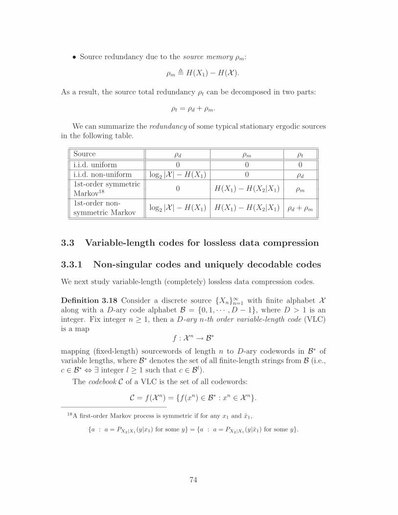
• Source redundancy due to the source memory ρm:
ρm , H(X1) − H(X ).
As a result, the source total redundancy ρt can be decomposed in two parts:
ρt = ρd + ρm.
We can summarize the redundancy of some typical stationary ergodic sourcesin the following table.
Source ρd ρm ρt
i.i.d. uniform 0 0 0i.i.d. non-uniform log2 |X | − H(X1) 0 ρd
1st-order symmetricMarkov18 0 H(X1) − H(X2|X1) ρm
1st-order non-symmetric Markov
log2 |X | − H(X1) H(X1) − H(X2|X1) ρd + ρm
3.3 Variable-length codes for lossless data compression
3.3.1 Non-singular codes and uniquely decodable codes
We next study variable-length (completely) lossless data compression codes.
Definition 3.18 Consider a discrete source Xn∞n=1 with finite alphabet Xalong with a D-ary code alphabet B = 0, 1, · · · , D − 1, where D > 1 is aninteger. Fix integer n ≥ 1, then a D-ary n-th order variable-length code (VLC)is a map
f : X n → B∗
mapping (fixed-length) sourcewords of length n to D-ary codewords in B∗ ofvariable lengths, where B∗ denotes the set of all finite-length strings from B (i.e.,c ∈ B∗ ⇔ ∃ integer l ≥ 1 such that c ∈ Bl).
The codebook C of a VLC is the set of all codewords:
C = f(X n) = f(xn) ∈ B∗ : xn ∈ X n.
18A first-order Markov process is symmetric if for any x1 and x1,
a : a = PX2|X1(y|x1) for some y = a : a = PX2|X1
(y|x1) for some y.
74
A variable-length lossless data compression code is a code in which thesource symbols can be completely reconstructed without distortion. In orderto achieve this goal, the source symbols have to be encoded unambiguously inthe sense that any two different source symbols (with positive probabilities) arerepresented by different codewords. Codes satisfying this property are callednon-singular codes. In practice however, the encoder often needs to encode asequence of source symbols, which results in a concatenated sequence of code-words. If any concatenation of codewords can also be unambiguously recon-structed without punctuation, then the code is said to be uniquely decodable. Inother words, a VLC is uniquely decodable if all finite sequences of sourcewords(xn ∈ X n) are mapped onto distinct strings of codewords; i.e., for any m andm′, (xn
1 , xn2 , · · · , xn
m) 6= (yn1 , yn
2 , · · · , ynm′) implies that
(f(xn1 ), f(xn
2 ), · · · , f(xnm)) 6= (f(yn
1 ), f(yn2 ), · · · , f(yn
m′)).
Note that a non-singular VLC is not necessarily uniquely decodable. For exam-ple, consider a binary (first-order) code for the source with alphabet
X = A,B,C,D,E, F
given by
code of A = 0,
code of B = 1,
code of C = 00,
code of D = 01,
code of E = 10,
code of F = 11.
The above code is clearly non-singular; it is however not uniquely decodablebecause the codeword sequence, 010, can be reconstructed as ABA, DA or AE(i.e., (f(A), f(B), f(A)) = (f(D), f(A)) = (f(A), f(E)) even if (A,B,A), (D,A)and (A,E) are all non-equal).
One important objective is to find out how “efficiently” we can representa given discrete source via a uniquely decodable n-th order VLC and providea construction technique that (at least asymptotically, as n → ∞) attains theoptimal “efficiency.” In other words, we want to determine what is the smallestpossible average code rate (or equivalently, average codeword length) can ann-th order uniquely decodable VLC have when (losslessly) representing a givensource, and we want to give an explicit code construction that can attain thissmallest possible rate (at least asymptotically in the sourceword length n).
75
Definition 3.19 Let C be a D-ary n-th order VLC
f : X n → 0, 1, · · · , D − 1∗
for a discrete source Xn∞n=1 with alphabet X and distribution PXn(xn), xn ∈X n. Setting ℓ(cxn) as the length of the codeword cxn = f(xn) associated withsourceword xn, then the average codeword length for C is given by
ℓ ,∑
xn∈Xn
PXn(xn)ℓ(cxn)
and its average code rate (in D-ary code symbols/source symbol) is given by
Rn ,ℓ
n=
1
n
∑
xn∈Xn
PXn(xn)ℓ(cxn).
The following theorem provides a strong condition which a uniquely decod-able code must satisfy.
Theorem 3.20 (Kraft inequality for uniquely decodable codes) Let C bea uniquely decodable D-ary n-th order VLC for a discrete source Xn∞n=1 withalphabet X . Let the M = |X |n codewords of C have lengths ℓ1, ℓ2, . . . , ℓM ,respectively. Then the following inequality must hold
M∑
m=1
D−ℓm ≤ 1.
Proof: Suppose that we use the codebook C to encode N sourcewords (xni ∈
X n, i = 1, · · · , N) arriving in a sequence; this yields a concatenated codewordsequence
c1c2c3 . . . cN .
Let the lengths of the codewords be respectively denoted by
ℓ(c1), ℓ(c2), . . . , ℓ(cN).
Consider (∑
c1∈C
∑
c2∈C· · ·∑
cN∈CD−[ℓ(c1)+ℓ(c2)+···+ℓ(cN )]
)
.
It is obvious that the above expression is equal to
(∑
c∈CD−ℓ(c)
)N
=
(M∑
m=1
D−ℓm
)N
.
76

(Note that |C| = M .) On the other hand, all the code sequences with length
i = ℓ(c1) + ℓ(c2) + · · · + ℓ(cN)
contribute equally to the sum of the identity, which is D−i. Let Ai denote thenumber of N -codeword sequences that have length i. Then the above identitycan be re-written as
(M∑
m=1
D−ℓm
)N
=LN∑
i=1
AiD−i,
whereL , max
c∈Cℓ(c).
Since C is by assumption a uniquely decodable code, the codeword sequencemust be unambiguously decodable. Observe that a code sequence with length ihas at most Di unambiguous combinations. Therefore, Ai ≤ Di, and
(M∑
m=1
D−ℓm
)N
=LN∑
i=1
AiD−i ≤
LN∑
i=1
DiD−i = LN,
which implies thatM∑
m=1
D−ℓm ≤ (LN)1/N .
The proof is completed by noting that the above inequality holds for every N ,and the upper bound (LN)1/N goes to 1 as N goes to infinity. 2
The Kraft inequality is a very useful tool, especially for showing that thefundamental lower bound of the average rate of uniquely decodable VLCs fordiscrete memoryless sources is given by the source entropy.
Theorem 3.21 The average rate of every uniquely decodable D-ary n-th orderVLC for a discrete memoryless source Xn∞n=1 is lower-bounded by the sourceentropy HD(X) (measured in D-ary code symbols/source symbol).
Proof: Consider a uniquely decodable D-ary n-th order VLC code for the sourceXn∞n=1
f : X n → 0, 1, · · · , D − 1∗
and let ℓ(cxn) denote the length of the codeword cxn = f(xn) for sourceword xn.Hence,
Rn − HD(X) =1
n
∑
xn∈Xn
PXn(xn)ℓ(cxn) − 1
nHD(Xn)
77

=1
n
[∑
xn∈Xn
PXn(xn)ℓ(cxn) −∑
xn∈Xn
(−PXn(xn) logD PXn(xn))
]
=1
n
∑
xn∈Xn
PXn(xn) logD
PXn(xn)
D−ℓ(cxn )
≥ 1
n
[∑
xn∈Xn
PXn(xn)
]
logD
[∑
xn∈Xn PXn(xn)]
[∑
xn∈Xn D−ℓ(cxn)]
(log-sum inequality)
= − 1
nlog
[∑
xn∈Xn
D−ℓ(cxn )
]
≥ 0
where the last inequality follows from the Kraft inequality for uniquely decodablecodes and the fact that the logarithm is a strictly increasing function. 2
By examining the above proof, we observe that
Rn = HD(X) iff PXn(xn) = D−l(cxn);
i.e., the source symbol probabilities are (negative) integer powers of D. Such asource is called D-adic [57]. In this case, the code is called absolutely optimal asit achieves the source entropy lower bound (it is thus optimal in terms of yieldinga minimal average code rate for any given n).
Furthermore, we know from the above theorem that the average code rateis no smaller than the source entropy. Indeed a lossless data compression code,whose average code rate achieves entropy, should be optimal (since if its averagecode rate is below entropy, the Kraft inequality is violated and the code is nolonger uniquely decodable). We summarize
1. Uniquely decodability ⇒ the Kraft inequality holds.
2. Uniquely decodability ⇒ average code rate of VLCs for memoryless sourcesis lower bounded by the source entropy.
Exercise 3.22
1. Find a non-singular and also non-uniquely decodable code that violates theKraft inequality. (Hint: The answer is already provided in this subsection.)
2. Find a non-singular and also non-uniquely decodable code that beats theentropy lower bound.
78

Prefixcodes
Uniquelydecodable codes
Non-singularcodes
Figure 3.4: Classification of variable-length codes.
3.3.2 Prefix or instantaneous codes
A prefix code is a VLC which is self-punctuated in the sense that there is noneed to append extra symbols for differentiating adjacent codewords. A moreprecise definition follows:
Definition 3.23 (Prefix code) A VLC is called a prefix code or an instanta-neous code if no codeword is a prefix of any other codeword.
A prefix code is also named an instantaneous code because the codeword se-quence can be decoded instantaneously (it is immediately recognizable) withoutthe reference to future codewords in the same sequence. Note that a uniquelydecodable code is not necessarily prefix-free and may not be decoded instanta-neously. The relationship between different codes encountered thus far is de-picted in Figure 3.4.
A D-ary prefix code can be represented graphically as an initial segment ofa D-ary tree. An example of a tree representation for a binary (D = 2) prefixcode is shown in Figure 3.5.
Theorem 3.24 (Kraft inequality for prefix codes) There exists a D-arynth-order prefix code for a discrete source Xn∞n=1 with alphabet X iff the code-words of length ℓm, m = 1, . . . ,M , satisfy the Kraft inequality, where M = |X |n.
Proof: Without loss of generality, we provide the proof for the case of D = 2(binary codes).
1. [The forward part] Prefix codes satisfy the Kraft inequality.
The codewords of a prefix code can always be put on a tree. Pick up a length
ℓmax , max1≤m≤M
ℓm.
79

U
R
R
R*
j
(0)
(1)
00
01
10
(11)
110
(111) 1110
1111
Figure 3.5: Tree structure of a binary prefix code. The codewords arethose residing on the leaves, which in this case are 00, 01, 10, 110, 1110and 1111.
A tree has originally 2ℓmax nodes on level ℓmax. Each codeword of length ℓm
obstructs 2ℓmax−ℓm nodes on level ℓmax. In other words, when any node is chosenas a codeword, all its children will be excluded from being codewords (as for aprefix code, no codeword can be a prefix of any other code). There are exactly2ℓmax−ℓm excluded nodes on level ℓmax of the tree. We therefore say that eachcodeword of length ℓm obstructs 2ℓmax−ℓm nodes on level ℓmax. Note that no twocodewords obstruct the same nodes on level ℓmax. Hence the number of totallyobstructed codewords on level ℓmax should be less than 2ℓmax , i.e.,
M∑
m=1
2ℓmax−ℓm ≤ 2ℓmax ,
which immediately implies the Kraft inequality:
M∑
m=1
2−ℓm ≤ 1.
(This part can also be proven by stating the fact that a prefix code is a uniquelydecodable code. The objective of adding this proof is to illustrate the character-istics of a tree-like prefix code.)
80
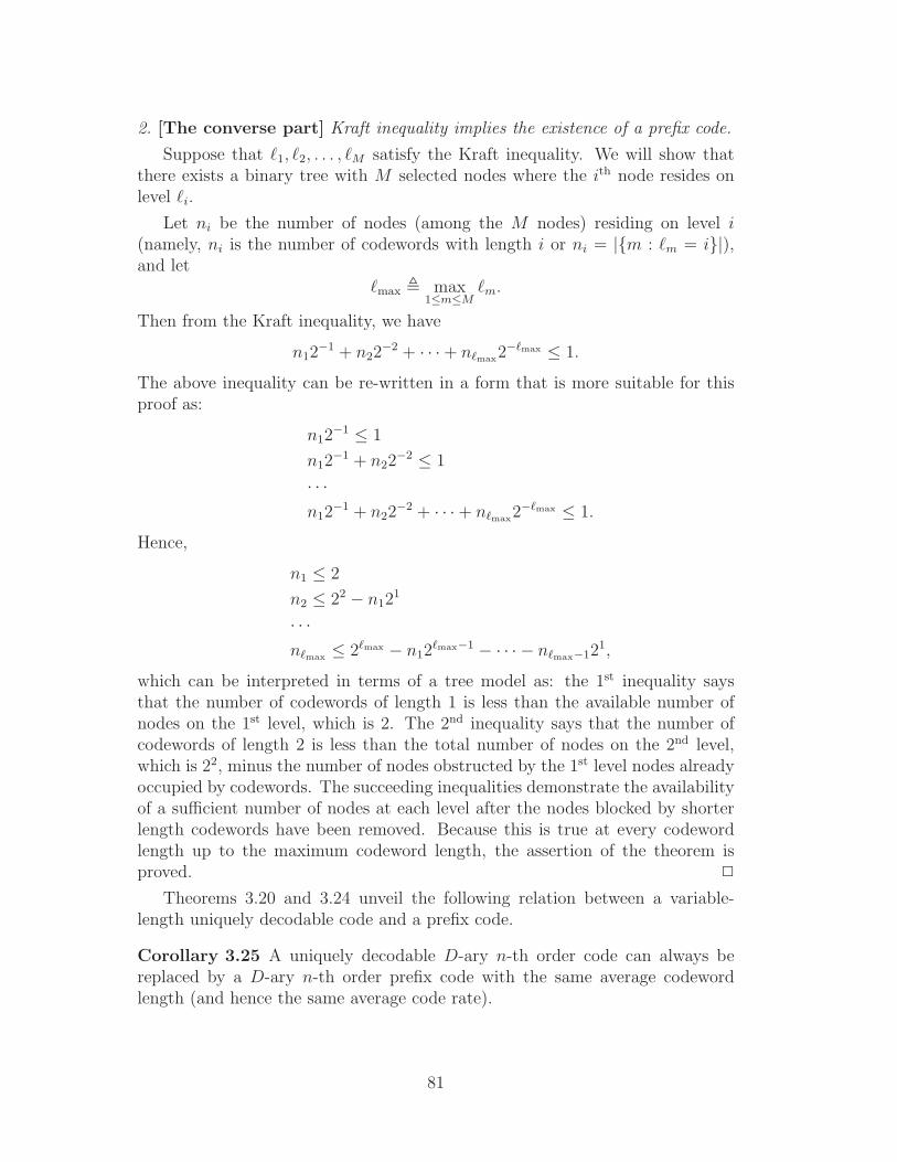
2. [The converse part] Kraft inequality implies the existence of a prefix code.
Suppose that ℓ1, ℓ2, . . . , ℓM satisfy the Kraft inequality. We will show thatthere exists a binary tree with M selected nodes where the ith node resides onlevel ℓi.
Let ni be the number of nodes (among the M nodes) residing on level i(namely, ni is the number of codewords with length i or ni = |m : ℓm = i|),and let
ℓmax , max1≤m≤M
ℓm.
Then from the Kraft inequality, we have
n12−1 + n22
−2 + · · · + nℓmax2−ℓmax ≤ 1.
The above inequality can be re-written in a form that is more suitable for thisproof as:
n12−1 ≤ 1
n12−1 + n22
−2 ≤ 1
· · ·n12
−1 + n22−2 + · · · + nℓmax2
−ℓmax ≤ 1.
Hence,
n1 ≤ 2
n2 ≤ 22 − n121
· · ·nℓmax ≤ 2ℓmax − n12
ℓmax−1 − · · · − nℓmax−121,
which can be interpreted in terms of a tree model as: the 1st inequality saysthat the number of codewords of length 1 is less than the available number ofnodes on the 1st level, which is 2. The 2nd inequality says that the number ofcodewords of length 2 is less than the total number of nodes on the 2nd level,which is 22, minus the number of nodes obstructed by the 1st level nodes alreadyoccupied by codewords. The succeeding inequalities demonstrate the availabilityof a sufficient number of nodes at each level after the nodes blocked by shorterlength codewords have been removed. Because this is true at every codewordlength up to the maximum codeword length, the assertion of the theorem isproved. 2
Theorems 3.20 and 3.24 unveil the following relation between a variable-length uniquely decodable code and a prefix code.
Corollary 3.25 A uniquely decodable D-ary n-th order code can always bereplaced by a D-ary n-th order prefix code with the same average codewordlength (and hence the same average code rate).
81

The following theorem interprets the relationship between the average coderate of a prefix code and the source entropy.
Theorem 3.26 Consider a discrete memoryless source Xn∞n=1.
1. For any D-ary n-th order prefix code for the source, the average code rateis no less than the source entropy HD(X).
2. There must exist a D-ary n-th order prefix code for the source whoseaverage code rate is no greater than HD(X) + 1
n, namely,
Rn ,1
n
∑
xn∈Xn
PXn(xn)ℓ(cxn) ≤ HD(X) +1
n, (3.3.1)
where cxn is the codeword for sourceword xn, and ℓ(cxn) is the length ofcodeword cxn .
Proof: A prefix code is uniquely decodable, and hence it directly follows fromTheorem 3.21 that its average code rate is no less than the source entropy.
To prove the second part, we can design a prefix code satisfying both (3.3.1)and the Kraft inequality, which immediately implies the existence of the desiredcode by Theorem 3.24. Choose the codeword length for sourceword xn as
ℓ(cxn) = ⌊− logD PXn(xn)⌋ + 1. (3.3.2)
ThenD−ℓ(cxn ) ≤ PXn(xn).
Summing both sides over all source symbols, we obtain
∑
xn∈Xn
D−ℓ(cxn) ≤ 1,
which is exactly the Kraft inequality. On the other hand, (3.3.2) implies
ℓ(cxn) ≤ − logD PXn(xn) + 1,
which in turn implies
∑
xn∈Xn
PXn(xn)ℓ(cxn) ≤∑
xn∈Xn
[− PXn(xn) logD PXn(xn)
]+∑
xn∈Xn
PXn(xn)
= HD(Xn) + 1 = nHD(X) + 1,
where the last equality holds since the source is memoryless. 2
82
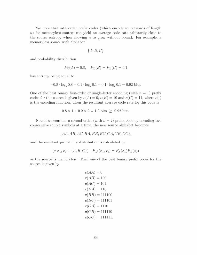
We note that n-th order prefix codes (which encode sourcewords of lengthn) for memoryless sources can yield an average code rate arbitrarily close tothe source entropy when allowing n to grow without bound. For example, amemoryless source with alphabet
A,B,C
and probability distribution
PX(A) = 0.8, PX(B) = PX(C) = 0.1
has entropy being equal to
−0.8 · log2 0.8 − 0.1 · log2 0.1 − 0.1 · log2 0.1 = 0.92 bits.
One of the best binary first-order or single-letter encoding (with n = 1) prefixcodes for this source is given by c(A) = 0, c(B) = 10 and c(C) = 11, where c(·)is the encoding function. Then the resultant average code rate for this code is
0.8 × 1 + 0.2 × 2 = 1.2 bits ≥ 0.92 bits.
Now if we consider a second-order (with n = 2) prefix code by encoding twoconsecutive source symbols at a time, the new source alphabet becomes
AA,AB,AC,BA,BB,BC,CA,CB,CC,
and the resultant probability distribution is calculated by
(∀ x1, x2 ∈ A,B,C) PX2(x1, x2) = PX(x1)PX(x2)
as the source is memoryless. Then one of the best binary prefix codes for thesource is given by
c(AA) = 0
c(AB) = 100
c(AC) = 101
c(BA) = 110
c(BB) = 111100
c(BC) = 111101
c(CA) = 1110
c(CB) = 111110
c(CC) = 111111.
83

The average code rate of this code now becomes
0.64(1 × 1) + 0.08(3 × 3 + 4 × 1) + 0.01(6 × 4)
2= 0.96 bits,
which is closer to the source entropy of 0.92 bits. As n increases, the averagecode rate will be brought closer to the source entropy.
From Theorems 3.21 and 3.26, we obtain the lossless variable-length sourcecoding theorem for discrete memoryless sources.
Theorem 3.27 (Lossless variable-length source coding theorem) Fix in-teger D > 1 and consider a DMS Xn∞n=1 with distribution PX and entropyHD(X) (measured in D-ary units). Then the following hold.
• Forward part (achievability): For any ε > 0, there exists a D-ary n-thorder prefix (hence uniquely decodable) code
f : X n → 0, 1, · · · , D − 1∗
for the source with an average code rate Rn satisfying
Rn ≤ HD(X) + ε
for n sufficiently large.
• Converse part: Every uniquely decodable code
f : X n → 0, 1, · · · , D − 1∗
for the source has an average code rate Rn ≥ HD(X).
Thus, for a discrete memoryless source, its entropy HD(X) (measured in D-ary units) represents the smallest variable-length lossless compression rate for nsufficiently large.
Proof: The forward part follows directly from Theorem 3.26 by choosingn large enough such that 1/n < ε, and the converse part is already given byTheorem 3.21. 2
Observation 3.28 Theorem 3.27 actually also holds for the class of stationarysources by replacing the source entropy HD(X) with the source entropy rate
HD(X ) , limn→∞
1
nHD(Xn),
measured in D-ary units. The proof is very similar to the proofs of Theorems 3.21and 3.26 with slight modifications (such as using the fact that 1
nHD(Xn) is non-
increasing with n for stationary sources).
84
Observation 3.29 (Renyi’s entropy and lossless data compression) Inthe lossless variable-length source coding theorem, we have chosen the crite-rion of minimizing the average codeword length. Implicit in the use of averagecodeword length as a performance criterion is the assumption that the cost ofcompression varies linearly with codeword length. This is not always the caseas in some applications, where the processing cost of decoding may be elevatedand buffer overflows caused by long codewords can cause problems, an exponen-tial cost/penalty function for codeword lengths can be more appropriate than alinear cost function [44, 150, 37]. Naturally, one would desire to choose a gener-alized function with exponential costs such that the familiar linear cost function(given by the average codeword length) is a special limiting case.
Indeed in [44], given a D-ary n-th order VLC C
f : X n → 0, 1, · · · , D − 1∗
for a discrete source Xi∞n=1 with alphabet X and distribution PXn , Campbellconsiders the following exponential cost function, called the average codewordlength of order t:
Ln(t) ,1
tlogD
(∑
xn∈Xn
PXn(xn)Dt·ℓ(cxn )
)
,
where t is a chosen positive constant, cxn = f(xn) is the codeword associatedwith sourceword xn and ℓ(·) is the length of cxn . Similarly, 1
nLn(t) denotes the
average code rate of order t. The criterion for optimality now becomes that ann-th order code is said to be optimal if its cost Ln(t) is the smallest among allpossible uniquely decodable codes.
In the limiting case when t → 0, Ln(0) → ∑
x∈X PX(x)ℓ(cx) = ℓ and werecover the average codeword length, as desired. Also, when t → ∞, Ln(∞) →maxx∈X ℓ(cx), which is the maximum codeword length for all codewords inC. Note that for a fixed t > 0, minimizing Ln(t) is equivalent to minimizing∑
xn∈Xn PXn(xn)Dtℓ(cxn ). In this sum, the weight for codeword cxn is Dtℓ(cxn )
and hence smaller codeword lengths are favored.
For this source coding setup with an exponential cost function, Campbellestablished in [44] an operational characterization for Renyi’s entropy by provingthe following lossless variable-length coding theorem for memoryless sources.
Theorem 3.30 (Lossless source coding theorem under exponential costs)Consider a DMS Xn with Renyi entropy in D-ary units and of order α givenby
Hα(X) =1
1 − αlogD
(∑
x∈XPα
X(x)
)
.
85

Fixing t > 0 and setting α = 11+t
, the following hold.
• For any ε > 0, there exists a D-ary n-th order uniquely decodable codef : X n → 0, 1, · · · , D − 1∗ for the source with an average code rate oforder t satisfying
1
nLn(t) ≤ Hα(X) + ε
for n sufficiently large.
• Conversely, it is not possible to find a uniquely decodable code whoseaverage code rate of order t is less than Hα(X).
Noting (by Lemma 2.50) that the Renyi entropy of order α reduces to theShannon entropy (in D-ary units) as α → 1, the above theorem reduces toTheorem 3.27 as α → 1 (or equivalently, as t → 0). Finally, in [220, Sec-tion 4.4], [221, 222], the above source coding theorem is extended for time-invariant Markov sources in terms of the Renyi entropy rate, limn→∞
1nHα(Xn)
with α = (1 + t)−1, which exists and can be calculated in closed-form for suchsources.
3.3.3 Examples of binary prefix codes
A) Huffman codes: optimal variable-length codes
Given a discrete source with alphabet X , we next construct an optimal binaryfirst-order (single-letter) uniquely decodable variable-length code
f : X → 0, 1∗,where optimality is in the sense that the code’s average codeword length (orequivalently, its average code rate) is minimized over the class of all binaryuniquely decodable codes for the source. Note that finding optimal n-th odercodes with n > 1 follows directly by considering X n as a new source with ex-panded alphabet (i.e., by mapping n source symbols at a time).
By Corollary 3.25, we remark that in our search for optimal uniquely de-codable codes, we can restrict our attention to the (smaller) class of optimalprefix codes. We thus proceed by observing the following necessary conditionsof optimality for binary prefix codes.
Lemma 3.31 Let C be an optimal binary prefix code with codeword lengthsℓi, i = 1, · · · ,M , for a source with alphabet X = a1, . . . , aM and symbolprobabilities p1, . . . , pM . We assume, without loss of generality, that
p1 ≥ p2 ≥ p3 ≥ · · · ≥ pM ,
86

and that any group of source symbols with identical probability is listed in orderof increasing codeword length (i.e., if pi = pi+1 = · · · = pi+s, then ℓi ≤ ℓi+1 ≤· · · ≤ ℓi+s). Then the following properties hold.
1. Higher probability source symbols have shorter codewords: pi > pj impliesℓi ≤ ℓj, for i, j = 1, · · · ,M .
2. The two least probable source symbols have codewords of equal length:ℓM−1 = ℓM .
3. Among the codewords of length ℓM , two of the codewords are identicalexcept in the last digit.
Proof:
1) If pi > pj and ℓi > ℓj, then it is possible to construct a better code C′ byinterchanging (“swapping”) codewords i and j of C, since
ℓ(C′) − ℓ(C) = piℓj + pjℓi − (piℓi + pjℓj)
= (pi − pj)(ℓj − ℓi)
< 0.
Hence code C′ is better than code C, contradicting the fact that C is optimal.
2) We first know that ℓM−1 ≤ ℓM , since:
• If pM−1 > pM , then ℓM−1 ≤ ℓM by result 1) above.
• If pM−1 = pM , then ℓM−1 ≤ ℓM by our assumption about the orderingof codewords for source symbols with identical probability.
Now, if ℓM−1 < ℓM , we may delete the last digit of codeword M , and thedeletion cannot result in another codeword since C is a prefix code. Thusthe deletion forms a new prefix code with a better average codeword lengththan C, contradicting the fact that C is optimal. Hence, we must have thatℓM−1 = ℓM .
3) Among the codewords of length ℓM , if no two codewords agree in all digitsexcept the last, then we may delete the last digit in all such codewords toobtain a better codeword. 2
The above observation suggests that if we can construct an optimal code forthe entire source except for its two least likely symbols, then we can constructan optimal overall code. Indeed, the following lemma due to Huffman followsfrom Lemma 3.31.
87

Lemma 3.32 (Huffman) Consider a source with alphabet X = a1, . . . , aMand symbol probabilities p1, . . . , pM such that p1 ≥ p2 ≥ · · · ≥ pM . Consider thereduced source alphabet Y obtained from X by combining the two least likelysource symbols aM−1 and aM into an equivalent symbol aM−1,M with probabilitypM−1 + pM . Suppose that C′, given by f ′ : Y → 0, 1∗, is an optimal code forthe reduced source Y . We now construct a code C, f : X → 0, 1∗, for theoriginal source X as follows:
• The codewords for symbols a1, a2, · · · , aM−2 are exactly the same as thecorresponding codewords in C′:
f(a1) = f ′(a1), f(a2) = f ′(a2), · · · , f(aM−2) = f ′(aM−2).
• The codewords associated with symbols aM−1 and aM are formed by ap-pending a “0” and a “1”, respectively, to the codeword f ′(aM−1,M) associ-ated with the letter aM−1,M in C′:
f(aM−1) = [f ′(aM−1,M)0] and f(aM) = [f ′(aM−1,M)1].
Then code C is optimal for the original source X .
Hence the problem of finding the optimal code for a source of alphabet sizeM is reduced to the problem of finding an optimal code for the reduced sourceof alphabet size M − 1. In turn we can reduce the problem to that of size M − 2and so on. Indeed the above lemma yields a recursive algorithm for constructingoptimal binary prefix codes.
Huffman encoding algorithm: Repeatedly apply the above lemma until one is leftwith a reduced source with two symbols. An optimal binary prefix code for thissource consists of the codewords 0 and 1. Then proceed backwards, constructing(as outlined in the above lemma) optimal codes for each reduced source untilone arrives at the original source.
Example 3.33 Consider a source with alphabet
X = 1, 2, 3, 4, 5, 6
and symbol probabilities 0.25, 0.25, 0.25, 0.1, 0.1 and 0.05, respectively. By fol-lowing the Huffman encoding procedure as shown in Figure 3.6, we obtain theHuffman code as
00, 01, 10, 110, 1110, 1111.
88
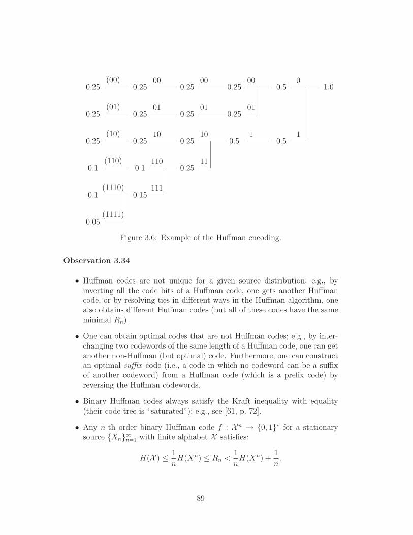
0.05
0.1
0.1
0.25
0.25
0.25
(1111)
(1110)
(110)
(10)
(01)
(00)
0.15
0.1
0.25
0.25
0.25
111
110
10
01
00
0.25
0.25
0.25
0.25
11
10
01
00
0.5
0.25
0.25
1
01
00
0.5
0.5
1
01.0
Figure 3.6: Example of the Huffman encoding.
Observation 3.34
• Huffman codes are not unique for a given source distribution; e.g., byinverting all the code bits of a Huffman code, one gets another Huffmancode, or by resolving ties in different ways in the Huffman algorithm, onealso obtains different Huffman codes (but all of these codes have the sameminimal Rn).
• One can obtain optimal codes that are not Huffman codes; e.g., by inter-changing two codewords of the same length of a Huffman code, one can getanother non-Huffman (but optimal) code. Furthermore, one can constructan optimal suffix code (i.e., a code in which no codeword can be a suffixof another codeword) from a Huffman code (which is a prefix code) byreversing the Huffman codewords.
• Binary Huffman codes always satisfy the Kraft inequality with equality(their code tree is “saturated”); e.g., see [61, p. 72].
• Any n-th order binary Huffman code f : X n → 0, 1∗ for a stationarysource Xn∞n=1 with finite alphabet X satisfies:
H(X ) ≤ 1
nH(Xn) ≤ Rn <
1
nH(Xn) +
1
n.
89

Thus, as n increases to infinity, Rn → H(X ) but the complexity as well asencoding-decoding delay grows exponentially with n.
• Note that non-binary (i.e., for D > 2) Huffman codes can also be con-structed in a mostly similar way as for the case of binary Huffman codesby designing a D-ary tree and iteratively applying Lemma 3.32, where nowthe D least likely source symbols are combined at each stage. The onlydifference from the case of binary Huffman codes is that we have to ensurethat we are ultimately left with D symbols at the last stage of the algo-rithm to guarantee the code’s optimality. This is remedied by expandingthe original source alphabet X by adding “dummy” symbols (each withzero probability) so that the alphabet size of the expanded source |X ′| isthe smallest positive integer greater than or equal to |X | with
|X ′| = 1 (modulo D − 1).
For example, if |X | = 6 and D = 3 (ternary codes), we obtain that |X ′| = 7,meaning that we need to enlarge the original source X by adding onedummy (zero-probability) source symbol.
We thus obtain that the necessary conditions for optimality of Lemma 3.31also hold for D-ary prefix codes when replacing X with the expandedsource X ′ and replacing “two” with “D” in the statement of the lemma.The resulting D-ary Huffman code will be an optimal code for the originalsource X (e.g., see [97, Chap. 3] and [188, Chap. 11]).
• Generalized Huffman codes under exponential costs: When the losslesscompression problem allows for exponential costs, as discussed in Observa-tion 3.29 and formalized in Theorem 3.30, a straightforward generalizationof Huffman’s algorithm, which minimizes the average code rate of order t,1nLn(t), can be obtained [141, Theorem 1′]. More specifically, while in Huff-
man’s algorithm, each new node (for a combined or equivalent symbol) isassigned weight pi + pj, where pi and pj are the lowest weights (probabil-ities) among the available nodes, in the generalized algorithm, each newnode is assigned weight 2t(pi + pj). With this simple modification, onecan directly construct such generalized Huffman codes (e.g., see [221] forexamples of codes designed for Markov sources).
B) Shannon-Fano-Elias code
Assume X = 1, . . . ,M and PX(x) > 0 for all x ∈ X . Define
F (x) ,∑
a≤x
PX(a),
90
and
F (x) ,∑
a<x
PX(a) +1
2PX(x).
Encoder: For any x ∈ X , express F (x) in decimal binary form, say
F (x) = .c1c2 . . . ck . . . ,
and take the first k (fractional) bits as the codeword of source symbol x, i.e.,
(c1, c2, . . . , ck),
where k , ⌈log2(1/PX(x))⌉ + 1.
Decoder: Given codeword (c1, . . . , ck), compute the cumulative sum of F (·) start-ing from the smallest element in 1, 2, . . . ,M until the first x satisfying
F (x) ≥ .c1 . . . ck.
Then x should be the original source symbol.
Proof of decodability: For any number a ∈ [0, 1], let [a]k denote the operationthat chops the binary representation of a after k bits (i.e., removing the (k+1)th
bit, the (k + 2)th bit, etc). Then
F (x) −[F (x)
]
k<
1
2k.
Since k = ⌈log2(1/PX(x))⌉ + 1,
1
2k≤ 1
2PX(x)
=
[∑
a<x
PX(a) +PX(x)
2
]
−∑
a≤x−1
PX(a)
= F (x) − F (x − 1).
Hence,
F (x − 1) =
[
F (x − 1) +1
2k
]
− 1
2k≤ F (x) − 1
2k<[F (x)
]
k.
In addition,F (x) > F (x) ≥
[F (x)
]
k.
Consequently, x is the first element satisfying
F (x) ≥ .c1c2 . . . ck.
91

Average codeword length:
ℓ =∑
x∈XPX(x)
⌈
log2
1
PX(x)
⌉
+ 1
<∑
x∈XPX(x) log2
1
PX(x)+ 2
= (H(X) + 2) bits.
Observation 3.35 The Shannon-Fano-Elias code is a prefix code.
3.3.4 Examples of universal lossless variable-length codes
In Section 3.3.3, we assume that the source distribution is known. Thus we canuse either Huffman codes or Shannon-Fano-Elias codes to compress the source.What if the source distribution is not a known priori? Is it still possible toestablish a completely lossless data compression code which is universally good(or asymptotically optimal) for all interested sources? The answer is affirma-tive. Two of the examples are the adaptive Huffman codes and the Lempel-Zivcodes (which unlike Huffman and Shannon-Fano-Elias codes map variable-lengthsourcewords onto codewords).
A) Adaptive Huffman code
A straightforward universal coding scheme is to use the empirical distribution(or relative frequencies) as the true distribution, and then apply the optimalHuffman code according to the empirical distribution. If the source is i.i.d.,the relative frequencies will converge to its true marginal probability. Therefore,such universal codes should be good for all i.i.d. sources. However, in order to getan accurate estimation of the true distribution, one must observe a sufficientlylong source sequence under which the coder will suffer a long delay. This can beimproved by using the adaptive universal Huffman code [98].
The working procedure of the adaptive Huffman code is as follows. Startwith an initial guess of the source distribution (based on the assumption thatthe source is DMS). As a new source symbol arrives, encode the data in terms ofthe Huffman coding scheme according to the current estimated distribution, andthen update the estimated distribution and the Huffman codebook according tothe newly arrived source symbol.
To be specific, let the source alphabet be X , a1, . . . , aM. Define
N(ai|xn) , number of ai occurrence in x1, x2, . . . , xn.
92

Then the (current) relative frequency of ai is N(ai|xn)/n. Let cn(ai) denotethe Huffman codeword of source symbol ai with respect to the distribution
[N(a1|xn)
n,N(a2|xn)
n, · · · ,
N(aM |xn)
n
]
.
Now suppose that xn+1 = aj. The codeword cn(aj) is set as output, and therelative frequency for each source outcome becomes:
N(aj|xn+1)
n + 1=
n × (N(aj|xn)/n) + 1
n + 1
andN(ai|xn+1)
n + 1=
n × (N(ai|xn)/n)
n + 1for i 6= j.
This observation results in the following distribution update policy:
P(n+1)
X(aj) =
nP(n)
X(aj) + 1
n + 1
andP
(n+1)
X(ai) =
n
n + 1P
(n)
X(ai) for i 6= j,
where P(n+1)
Xrepresents the estimate of the true distribution PX at time (n+1).
Note that in the Adaptive Huffman coding scheme, the encoder and decoderneed not be re-designed at every time, but only when a sufficient change in theestimated distribution occurs such that the so-called sibling property is violated.
Definition 3.36 (Sibling property) A prefix code is said to have the siblingproperty if its codetree satisfies:
1. every node in the code-tree (except for the root node) has a sibling (i.e.,the code-tree is saturated), and
2. the node can be listed in non-decreasing order of probabilities with eachnode being adjacent to its sibling.
The next observation indicates the fact that the Huffman code is the onlyprefix code satisfying the sibling property.
Observation 3.37 A prefix code is a Huffman code iff it satisfies the siblingproperty.
93
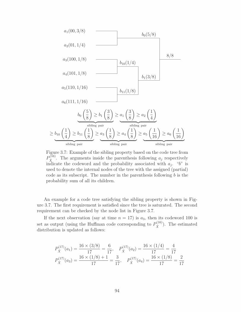
a1(00, 3/8)
a2(01, 1/4)
a3(100, 1/8)
a4(101, 1/8)
a5(110, 1/16)
a6(111, 1/16)
b11(1/8)
b10(1/4)
b0(5/8)
b1(3/8)
8/8
b0
(5
8
)
≥ b1
(3
8
)
︸ ︷︷ ︸
sibling pair
≥ a1
(3
8
)
≥ a2
(1
4
)
︸ ︷︷ ︸
sibling pair
≥ b10
(1
4
)
≥ b11
(1
8
)
︸ ︷︷ ︸
sibling pair
≥ a3
(1
8
)
≥ a4
(1
8
)
︸ ︷︷ ︸
sibling pair
≥ a5
(1
16
)
≥ a6
(1
16
)
︸ ︷︷ ︸
sibling pair
Figure 3.7: Example of the sibling property based on the code tree fromP
(16)
X. The arguments inside the parenthesis following aj respectively
indicate the codeword and the probability associated with aj. “b” isused to denote the internal nodes of the tree with the assigned (partial)code as its subscript. The number in the parenthesis following b is theprobability sum of all its children.
An example for a code tree satisfying the sibling property is shown in Fig-ure 3.7. The first requirement is satisfied since the tree is saturated. The secondrequirement can be checked by the node list in Figure 3.7.
If the next observation (say at time n = 17) is a3, then its codeword 100 is
set as output (using the Huffman code corresponding to P(16)
X). The estimated
distribution is updated as follows:
P(17)
X(a1) =
16 × (3/8)
17=
6
17, P
(17)
X(a2) =
16 × (1/4)
17=
4
17
P(17)
X(a3) =
16 × (1/8) + 1
17=
3
17, P
(17)
X(a4) =
16 × (1/8)
17=
2
17
94

a1(00, 6/17)
a2(01, 4/17)
a3(100, 3/17)
a4(101, 2/17)
a5(110, 1/17)
a6(111, 1/17)
b11(2/17)
b10(5/17)
b0(10/17)
b1(7/17)
17/17
b0
(10
17
)
≥ b1
(7
17
)
︸ ︷︷ ︸
sibling pair
≥ a1
(6
17
)
≥ b10
(5
17
)
≥ a2
(4
17
)
≥ a3
(3
17
)
≥ a4
(2
17
)
︸ ︷︷ ︸
sibling pair
≥ b11
(2
17
)
≥ a5
(1
17
)
≥ a6
(1
17
)
︸ ︷︷ ︸
sibling pair
Figure 3.8: (Continuation of Figure 3.7) Example of violation of thesibling property after observing a new symbol a3 at n = 17. Note thatnode a1 is not adjacent to its sibling a2.
P(17)
X(a5) =
16 × [1/(16)]
17=
1
17, P
(17)
X(a6) =
16 × [1/(16)]
17=
1
17.
The sibling property is then violated (cf. Figure 3.8). Hence, codebook needsto be updated according to the new estimated distribution, and the observationat n = 18 shall be encoded using the new codebook in Figure 3.9. Details aboutAdaptive Huffman codes can be found in [98].
B) Lempel-Ziv codes
We now introduce a well-known and feasible universal coding scheme, which isnamed after its inventors, Lempel and Ziv (e.g., cf. [57]). These codes, unlikeHuffman and Shannon-Fano-Elias codes, map variable-length sourcewords (asopposed to fixed-length codewords) onto codewords.
Suppose the source alphabet is binary. Then the Lempel-Ziv encoder can bedescribed as follows.
95

a1(10, 6/17)
a2(00, 4/17)
a3(01, 3/17)
a4(110, 2/17)
a5(1110, 1/17)
a6(1111, 1/17)
b111(2/17)
b11(4/17)
b0(7/17)
b1(10/17)17/17
b1
(10
17
)
≥ b0
(7
17
)
︸ ︷︷ ︸
sibling pair
≥ a1
(6
17
)
≥ b11
(4
17
)
︸ ︷︷ ︸
sibling pair
≥ a2
(4
17
)
≥ a3
(3
17
)
︸ ︷︷ ︸
sibling pair
≥ a4
(2
17
)
≥ b111
(2
17
)
︸ ︷︷ ︸
sibling pair
≥ a5
(1
17
)
≥ a6
(1
17
)
︸ ︷︷ ︸
sibling pair
Figure 3.9: (Continuation of Figure 3.8) Updated Huffman code. Thesibling property holds now for the new code.
Encoder:
1. Parse the input sequence into strings that have never appeared before. Forexample, if the input sequence is 1011010100010 . . ., the algorithm firstgrabs the first letter 1 and finds that it has never appeared before. So 1is the first string. Then the algorithm scoops the second letter 0 and alsodetermines that it has not appeared before, and hence, put it to be thenext string. The algorithm moves on to the next letter 1, and finds thatthis string has appeared. Hence, it hits another letter 1 and yields a newstring 11, and so on. Under this procedure, the source sequence is parsedinto the strings
1, 0, 11, 01, 010, 00, 10.
2. Let L be the number of distinct strings of the parsed source. Then weneed log2 L bits to index these strings (starting from one). In the above
96
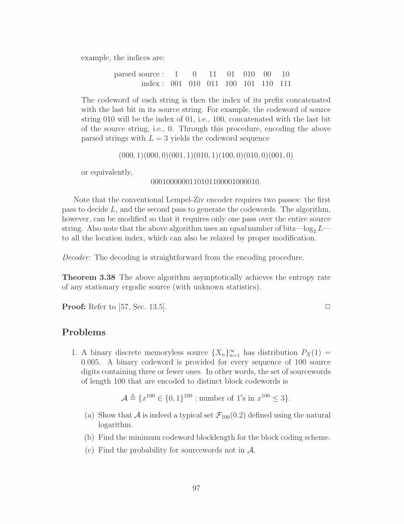
example, the indices are:
parsed source : 1 0 11 01 010 00 10index : 001 010 011 100 101 110 111
The codeword of each string is then the index of its prefix concatenatedwith the last bit in its source string. For example, the codeword of sourcestring 010 will be the index of 01, i.e., 100, concatenated with the last bitof the source string, i.e., 0. Through this procedure, encoding the aboveparsed strings with L = 3 yields the codeword sequence
(000, 1)(000, 0)(001, 1)(010, 1)(100, 0)(010, 0)(001, 0)
or equivalently,0001000000110101100001000010.
Note that the conventional Lempel-Ziv encoder requires two passes: the firstpass to decide L, and the second pass to generate the codewords. The algorithm,however, can be modified so that it requires only one pass over the entire sourcestring. Also note that the above algorithm uses an equal number of bits—log2 L—to all the location index, which can also be relaxed by proper modification.
Decoder: The decoding is straightforward from the encoding procedure.
Theorem 3.38 The above algorithm asymptotically achieves the entropy rateof any stationary ergodic source (with unknown statistics).
Proof: Refer to [57, Sec. 13.5]. 2
Problems
1. A binary discrete memoryless source Xn∞n=1 has distribution PX(1) =0.005. A binary codeword is provided for every sequence of 100 sourcedigits containing three or fewer ones. In other words, the set of sourcewordsof length 100 that are encoded to distinct block codewords is
A , x100 ∈ 0, 1100 : number of 1′s in x100 ≤ 3.
(a) Show that A is indeed a typical set F100(0.2) defined using the naturallogarithm.
(b) Find the minimum codeword blocklength for the block coding scheme.
(c) Find the probability for sourcewords not in A.
97

(d) Use Chebyshev’s inequality to bound the probability of observing asourceword outside A. Compare this bound with the actual probabi-lity computed in part (c).
Hint: Let Xi represent the binary random digit at instance i, and letSn = X1 + · · · + Xn. Note that Pr[S100 ≥ 4] is equal to
Pr
[∣∣∣∣
1
100S100 − 0.005
∣∣∣∣≥ 0.35
]
.
2. Weak converse to the Fixed-Length Source Coding Theorem: Recall (seeFootnote 3) that an (n,M) fixed-length source code for a discrete memo-ryless source (DMS) Xn∞n=1 with finite alphabet X consists of an encoderf : X n → 1, 2, · · · ,M, and a decoder g : 1, 2, · · · ,M → X n. The rateof the code is
Rn ,1
nlog2 M bits/source symbol,
and its probability of decoding error is
Pe = Pr[Xn 6= Xn],
where Xn = g(f(Xn)).
(a) Show that any fixed-length source code (n,M) for a DMS satisfies
Pe ≥H(X) − Rn
log2 |X | − 1
n log2 |X | ,
where H(X) is the source entropy.
Hint: Show that log2 M ≥ I(Xn; Xn), and use Fano’s inequality.
(b) Deduce the (weak) converse to the fixed-length source coding the-orem for DMS’s by proving that for any (n,M) source code withlim supn→∞ Rn < H(X), its Pe is bounded away from zero for n suf-ficiently large.
3. For a stationary source Xn∞n=1, show that for any integer n > 1,
(a) 1nH(Xn) ≤ 1
n−1H(Xn−1)
(b) 1nH(Xn) ≥ H(Xn|Xn−1).
Hint: Use the chain rule for entropy and the fact that
H(Xi|Xi−1, . . . , X1) = H(Xn|Xn−1, . . . , Xn−i+1)
for every i.
98
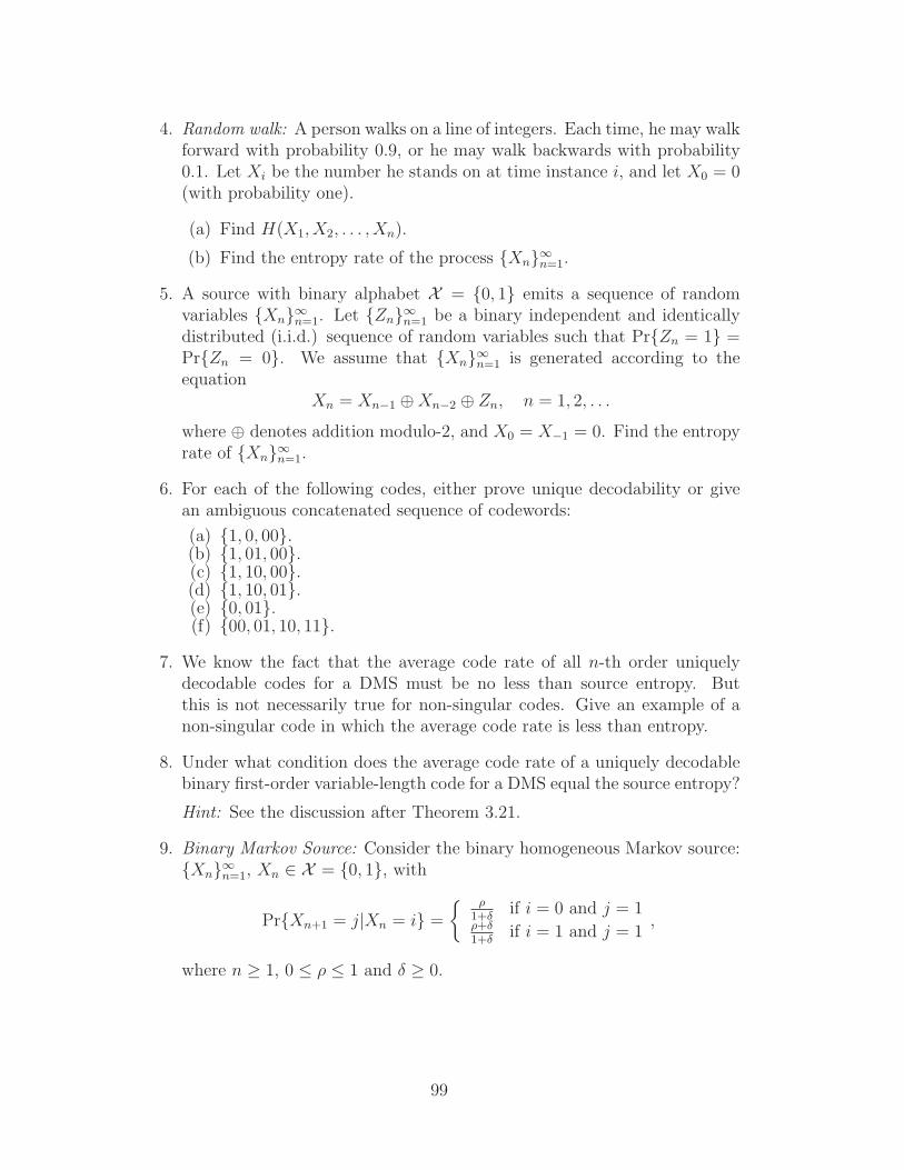
4. Random walk: A person walks on a line of integers. Each time, he may walkforward with probability 0.9, or he may walk backwards with probability0.1. Let Xi be the number he stands on at time instance i, and let X0 = 0(with probability one).
(a) Find H(X1, X2, . . . , Xn).
(b) Find the entropy rate of the process Xn∞n=1.
5. A source with binary alphabet X = 0, 1 emits a sequence of randomvariables Xn∞n=1. Let Zn∞n=1 be a binary independent and identicallydistributed (i.i.d.) sequence of random variables such that PrZn = 1 =PrZn = 0. We assume that Xn∞n=1 is generated according to theequation
Xn = Xn−1 ⊕ Xn−2 ⊕ Zn, n = 1, 2, . . .
where ⊕ denotes addition modulo-2, and X0 = X−1 = 0. Find the entropyrate of Xn∞n=1.
6. For each of the following codes, either prove unique decodability or givean ambiguous concatenated sequence of codewords:
(a) 1, 0, 00.(b) 1, 01, 00.(c) 1, 10, 00.(d) 1, 10, 01.(e) 0, 01.(f) 00, 01, 10, 11.
7. We know the fact that the average code rate of all n-th order uniquelydecodable codes for a DMS must be no less than source entropy. Butthis is not necessarily true for non-singular codes. Give an example of anon-singular code in which the average code rate is less than entropy.
8. Under what condition does the average code rate of a uniquely decodablebinary first-order variable-length code for a DMS equal the source entropy?
Hint: See the discussion after Theorem 3.21.
9. Binary Markov Source: Consider the binary homogeneous Markov source:Xn∞n=1, Xn ∈ X = 0, 1, with
PrXn+1 = j|Xn = i =
ρ1+δ
if i = 0 and j = 1ρ+δ1+δ
if i = 1 and j = 1,
where n ≥ 1, 0 ≤ ρ ≤ 1 and δ ≥ 0.
99

(a) Find the initial state distribution (PrX1 = 0, PrX1 = 1) requiredto make the source Xn∞n=1 stationary.
Assume in the next questions that the source is stationary.
(b) Find the entropy rate of Xn∞n=1 in terms of ρ and δ.
(c) If δ = 1 and ρ = 1/2, compute the source redundancies ρd, ρm and ρt.
(d) Suppose that ρ = 1. Is Xn∞n=1 irreducible? What is the value of theentropy rate in this case?
(e) If δ = 0, show that Xn∞n=1 is a discrete memoryless source andcompute its entropy rate in terms of ρ.
(f) If ρ = 1/2 and δ = 3/2, design first-, second-, and third-order binaryHuffman codes for this source. Determine in each case the averagecode rate and compare it to the entropy rate.
10. Polya contagion process of memory two: Consider the finite-memory Polyacontagion source presented in Example 3.16 with M = 2.
(a) Find the transition distribution of this binary Markov process and de-termine its stationary distribution in terms of the source parameters.
(b) Find the source entropy rate.
11. Suppose random variables Z1 and Z2 are independent from each other andhave the same distribution as Z with
Pr[Z = e1] = 0.4;Pr[Z = e2] = 0.3;Pr[Z = e3] = 0.2;Pr[Z = e4] = 0.1.
(a) Design a first-order binary Huffman code f : e1, e2, e3, e4 → 0, 1∗for Z.
(b) Applying the Huffman code in (a) to Z1 and Z2 and concatenatingf(Z1) with f(Z2) yields an overall codeword for the pair (Z1, Z2) givenby
f(Z1, Z2) , (f(Z1), f(Z2)) = (U1, U2, . . . , Uk),
where k ranges from 2 to 6, depending on the outcomes of Z1 and Z2.Are U1 and U2 independent? Justify your answer.
Hint: Examine Pr[U2 = 0|U1 = u1] for different values of u1.
(c) Is the average code rate equal to the entropy given by
0.4 log2
1
0.4+ 0.3 log2
1
0.3+ 0.2 log2
1
0.2
100

+ 0.1 log2
1
0.1= 1.84644 bits/letter?
Justify your answer.
(d) Now if we apply the Huffman code in (a) sequentially to the i.i.d. se-quence Z1, Z2, Z3, . . . with the same marginal distribution as Z, andyield the output U1, U2, U3, . . ., can U1, U2, U3, . . . be further com-pressed?
If your answer to this question is NO, prove the i.i.d. uniformity ofU1, U2, U3, . . .. If your answer to this question is YES, then explainwhy the optimal Huffman code does not give an i.i.d. uniform output.
Hint : Examine whether the average code rate can achieve sourceentropy.
12. In the second part of Theorem 3.26, it is shown that there exists a D-aryprefix code with
Rn =1
n
∑
x∈XPX(x)ℓ(cx) ≤ HD(X) +
1
n,
where cx is the codeword for the source symbol x and ℓ(cx) is the lengthof codeword cx. Show that the upper bound can be improved to:
Rn < HD(X) +1
n.
Hint: Replace ℓ(cx) = ⌊− logD PX(x)⌋ + 1 by a new assignment.
13. Let X1, X2, X3, · · · be an i.i.d. random variables with common alphabetx1, x2, x3, · · · , and assume that PX(xi) > 0 for every i.
(a) Prove that the average code rate of the first-order (single-letter) bi-nary Huffman code is equal to H(X) iff PX(xi) is equal to 2−ni forevery i, where nii≥1 is a sequence of positive integers.
Hint : The if-part can be proved by the new bound in Problem 12,and the only-if-part can be proved by modifying the proof of Theo-rem 3.21.
(b) What is the sufficient and necessary condition under which the aver-age code rate of the first-order (single-letter) ternary Huffman codeequals H3(X)?
(c) Prove that the average code rate of the second-order (two-letter) bi-nary Huffman code cannot be equal to H(X) + 1/2 bits?
Hint: Use the new bound in Problem 12.
101
14. Decide whether each of the following statements is true or false. Provethe validity of those that are true and give counterexamples or argumentsbased on known facts to disprove those that are false.
(a) Every Huffman code for a discrete memoryless source (DMS) has acorresponding suffix code with the same average code rate.
(b) Consider a DMS Xn∞n=1 with alphabet X = a1, a2, a3, a4, a5, a6and probability distribution
[p1, p2, p3, p4, p5, p6] =
[1
4,1
4,1
4,1
8,
1
16,
1
16
]
,
where pi , PrX = ai, i = 1, · · · , 6. The Shannon-Fano-Elias codef : X → 0, 1∗ for the source is optimal.
15. Consider a discrete memoryless source Xi∞i=1 with alphabet X = a, b, cand distribution P [X = a] = 1/2 and P [X = b] = P [X = c] = 1/4.
(a) Design an optimal first-order binary prefix code for this source (i.e.,for n = 1).
(b) Design an optimal second-order binary prefix code for this source (i.e.,for n = 2).
(c) Compare the codes in terms of both performance and complexity.Which code would you recommend ? Justify your answer.
16. The cost of miscoding [57]: Consider a discrete memoryless source Xn∞n=1
with alphabet X = a, b, c, d, e. Let p1(·) and p2(·) be two possible proba-bility mass functions for the source that are described in the table below.Also, let C1 = f1(X ) where f1 : X → 0, 1∗, and C2 = f2(X ) wheref2 : X → 0, 1∗, be two binary (first-order) prefix codes for the source asshown below.
Symbol x ∈ X p1(x) p2(x) f1(x) f2(x)a 1/2 1/2 0 0b 1/4 1/8 10 100c 1/8 1/8 110 101c 1/16 1/8 1110 110e 1/16 1/8 1111 111
(a) Calculate H(p1), H(p2), D(p1||p2) and D(p2||p1).
(b) Let R(Ci, pj) denote the average code rate of code Ci for the sourceunder distribution pj, i, j = 0, 1.
Calculate R(C1, p1), R(C1, p2), R(C2, p1), and R(C2, p2).
102

(c) Compare the quantities calculated in (b) to those in (a) and interpretthem qualitatively.
17. Consider a discrete memoryless source Xi∞i=1 with alphabet X and dis-tribution pX . Let C = f(X ) be a uniquely decodable binary code
f : X → 0, 1∗
that maps single source letters onto binary strings such that its averagecode rate RC satisfies
RC = H(X) bits/source symbol.
In other words, C is absolutely optimal.
Now consider a second binary code C′ = f ′(X n) for the source that mapssource n-tuples onto binary strings:
f ′ : X n → 0, 1∗.
Provide a construction for the map f ′ such that the code C′ is also abso-lutely optimal.
18. Consider two random variables X and Y with values in finite sets X andY , respectively. Let lX , lY and lXY denote the average codeword lengthsof the optimal (first-order) prefix codes
f : X → 0, 1∗,
g : Y → 0, 1∗
andh : X × Y → 0, 1∗,
respectively; i.e., lX = E[l(f(X))], lY = E[l(g(Y ))] and lXY = E[l(h(X,Y ))].
Prove that:
(a) lX + lY − lXY < I(X; Y ) + 2.
(b) lXY ≤ lX + lY .
19. Entropy rate [97]: Consider a discrete-time, finite-alphabet stationary ran-dom process Un∞n=1. Define
Hn|n(U) ,1
nH(U2n, · · · , Un+1|Un, · · · , U1).
103
(a) Show that Hn|n(U) is non-increasing in n.
(b) Prove that
limn→∞
Hn|n(U) = H(U),
where H(U) is the source entropy rate.
(c) Assume that the stationary source Un is also a Markov source.Compare Hn|n(U) to the source entropy rate H(U).
20. Divergence rate: Prove the expression in (3.2.6) for the divergence ratebetween a stationary source Xi and a time-invariant Markov source Xi,with both sources having a common finite alphabet X . Generalize theresult if the source Xi is a time-invariant k-th order Markov chain.
104

Chapter 4
Data Transmission and ChannelCapacity
4.1 Principles of data transmission
A noisy communication channel is an input-output medium in which the outputis not completely or deterministically specified by the input. The channel isindeed stochastically modeled, where given channel input x, the channel outputy is governed by a transition (conditional) probability distribution denoted byPY |X(y|x). Since two different inputs may give rise to the same output, thereceiver, upon receipt of an output, needs to guess the most probable sent in-put. In general, words of length n are sent and received over the channel; inthis case, the channel is characterized by a sequence of n-dimensional transitiondistributions PY n|Xn(yn|xn), for n = 1, 2, · · · . A block diagram depicting a datatransmission or channel coding system (with no output feedback) is given inFigure 4.1.
W - ChannelEncoder
-Xn ChannelPY n|Xn(·|·) -Y n
ChannelDecoder
-W
Figure 4.1: A data transmission system, where W represents the mes-sage for transmission, Xn denotes the codeword corresponding to mes-sage W , Y n represents the received word due to channel input Xn, andW denotes the reconstructed message from Y n.
The designer of a data transmission (or channel) code needs to carefully
105

select codewords from the set of channel input words (of a given length) sothat a minimal ambiguity is obtained at the channel receiver. For example,suppose that a channel has binary input and output alphabets and that itstransition probability distribution induces the following conditional probabilityon its output symbols given that input words of length 2 are sent:
PY |X2(y = 0|x2 = 00) = 1
PY |X2(y = 0|x2 = 01) = 1
PY |X2(y = 1|x2 = 10) = 1
PY |X2(y = 1|x2 = 11) = 1,
which can be graphically depicted as
*-
*-
11
10
01
00
1
01
1
1
1
and a binary message (either event A or event B) is required to be transmittedfrom the sender to the receiver. Then the data transmission code with (codeword00 for event A, codeword 10 for event B) obviously induces less ambiguity atthe receiver than the code with (codeword 00 for event A, codeword 01 for eventB).
In short, the objective in designing a data transmission (or channel) codeis to transform a noisy channel into a reliable medium for sending messagesand recovering them at the receiver with minimal loss. To achieve this goal, thedesigner of a data transmission code needs to take advantage of the common partsbetween the sender and the receiver sites that are least affected by the channelnoise. We will see that these common parts are probabilistically captured by themutual information between the channel input and the channel output.
As illustrated in the previous example, if a “least-noise-affected” subset ofthe channel input words is appropriately selected as the set of codewords, themessages intended to be transmitted can be reliably sent to the receiver witharbitrarily small error. One then raises the question:
What is the maximum amount of information (per channel use) thatcan be reliably transmitted over a given noisy channel ?
In the above example, we can transmit a binary message error-free, and hencethe amount of information that can be reliably transmitted is at least 1 bit
106

per channel use (or channel symbol). It can be expected that the amount ofinformation that can be reliably transmitted for a highly noisy channel shouldbe less than that for a less noisy channel. But such a comparison requires a goodmeasure of the “noisiness” of channels.
From an information theoretic viewpoint, “channel capacity” provides a goodmeasure of the noisiness of a channel; it represents the maximal amount of infor-mational messages (per channel use) that can be transmitted via a data trans-mission code over the channel and recovered with arbitrarily small probabilityof error at the receiver. In addition to its dependence on the channel transitiondistribution, channel capacity also depends on the coding constraint imposedon the channel input, such as “only block (fixed-length) codes are allowed.” Inthis chapter, we will study channel capacity for block codes (namely, only blocktransmission code can be used).1 Throughout the chapter, the noisy channel isassumed to be memoryless (as defined in the next section).
4.2 Discrete memoryless channels
Definition 4.1 (Discrete channel) A discrete communication channel is char-acterized by
• A finite input alphabet X .
• A finite output alphabet Y .
• A sequence of n-dimensional transition distributions
PY n|Xn(yn|xn)∞n=1
such that∑
yn∈Yn PY n|Xn(yn|xn) = 1 for every xn ∈ X n, where xn =(x1, · · · , xn) ∈ X n and yn = (y1, · · · , yn) ∈ Yn. We assume that the abovesequence of n-dimensional distribution is consistent, i.e.,
PY i|Xi(yi|xi) =
∑
xi+1∈X∑
yi+1∈Y PXi+1(xi+1)PY i+1|Xi+1(yi+1|xi+1)∑
xi+1∈X PXi+1(xi+1)
=∑
xi+1∈X
∑
yi+1∈YPXi+1|Xi(xi+1|xi)PY i+1|Xi+1(yi+1|xi+1)
for every xi, yi, PXi+1|Xi and i = 1, 2, · · · .
1See [281] for recent results regarding channel capacity when no coding constraints areapplied on the channel input (so that variable-length codes can be employed).
107

In general, real-world communications channels exhibit statistical memoryin the sense that current channel outputs statistically depend on past outputsas well as past, current and (possibly) future inputs. However, for the sake ofsimplicity, we restrict our attention in this chapter to the class of memorylesschannels (see Problem 4.27 for a brief discussion of channels with memory).
Definition 4.2 (Discrete memoryless channel) A discrete memoryless chan-nel (DMC) is a channel whose sequence of transition distributions PY n|Xn satisfies
PY n|Xn(yn|xn) =n∏
i=1
PY |X(yi|xi) (4.2.1)
for every n = 1, 2, · · · , xn ∈ X n and yn ∈ Yn. In other words, a DMC isfully described by the channel’s transition distribution matrix Q , [px,y] of size|X | × |Y|, where
px,y , PY |X(y|x)
for x ∈ X , y ∈ Y . Furthermore, the matrix Q is stochastic; i.e., the sum of theentries in each of its rows is equal to 1
(since
∑
y∈Y px,y = 1 for all x ∈ X).
Observation 4.3 We note that the DMC’s condition (4.2.1) is actually equiv-alent to the following two sets of conditions:
PYn|Xn,Y n−1(yn|xn, yn−1) = PY |X(yn|xn) ∀n = 1, 2, · · · , xn, yn;
(4.2.2a)
PY n−1|Xn(yn−1|xn) = PY n−1|Xn−1(yn−1|xn−1) ∀n = 2, 3, · · · , xn, yn−1.
(4.2.2b)
PYn|Xn,Y n−1(yn|xn, yn−1) = PY |X(yn|xn) ∀n = 1, 2, · · · , xn, yn;
(4.2.3a)
PXn|Xn−1,Y n−1(xn|xn−1, yn−1) = PXn|Xn−1(xn|xn−1) ∀n = 1, 2, · · · , xn, yn−1.
(4.2.3b)
Condition (4.2.2a) (also, (4.2.3a)) implies that the current output Yn only de-pends on the current input Xn but not on past inputs Xn−1 and outputs Y n−1.Condition (4.2.2b) indicates that the past outputs Y n−1 do not depend on thecurrent input Xn. These two conditions together give
PY n|Xn(yn|xn) = PY n−1|Xn(yn−1|xn)PYn|Xn,Y n−1(yn|xn, yn−1)
= PY n−1|Xn−1(yn−1|xn−1)PY |X(yn|xn);
hence, (4.2.1) holds recursively on n = 1, 2, · · · . The converse (i.e., (4.2.1) impliesboth (4.2.2a) and (4.2.2b)) is a direct consequence of
PYn|Xn,Y n−1(yn|xn, yn−1) =PY n|Xn(yn|xn)
∑
yn∈Y PY n|Xn(yn|xn)
108

andPY n−1|Xn(yn−1|xn) =
∑
yn∈YPY n|Xn(yn|xn).
Similarly, (4.2.3b) states that the current input Xn is independent of past outputsY n−1, which together with (4.2.3a) implies again
PY n|Xn(yn|xn)
=PXn,Y n(xn, yn)
PXn(xn)
=PXn−1,Y n−1(xn−1, yn−1)PXn|Xn−1,Y n−1(xn|xn−1, yn−1)PYn|Xn,Y n−1(yn|xn, yn−1)
PXn−1(xn−1)PXn|Xn−1(xn|xn−1)
= PY n−1|Xn−1(yn−1|xn−1)PY |X(yn|xn),
hence, recursively yielding (4.2.1). The converse for (4.2.3b)—i.e., (4.2.1) imply-ing (4.2.3b)— can be analogously proved by noting that
PXn|Xn−1,Y n−1(xn|xn−1, yn−1) =PXn(xn)
∑
yn∈Y PY n|Xn(yn|xn)
PXn−1(xn−1)PY n−1|Xn−1(yn−1|xn−1).
Note that the above definition of DMC in (4.2.1) prohibits the use of channelfeedback, as feedback allows the current channel input to be a function of pastchannel outputs (therefore, conditions (4.2.2b) and (4.2.3b) cannot hold withfeedback). Instead, a causality condition generalizing condition (4.2.2a) (e.g.,see Definition 7.4 in [294]) will be needed to define a channel with feedback.
Examples of DMCs:
1. Identity (noiseless) channels: An identity channel has equal-size input andoutput alphabets (|X | = |Y|) and channel transition probability satisfying
PY |X(y|x) =
1 if y = x
0 if y 6= x.
This is a noiseless or perfect channel as the channel input is received error-free at the channel output.
2. Binary symmetric channels: A binary symmetric channel (BSC) is a chan-nel with binary input and output alphabets such that each input has a(conditional) probability given by ε for being received inverted at the out-put, where ε ∈ [0, 1] is called the channel’s crossover probability or bit errorrate. The channel’s transition distribution matrix is given by
Q = [px,y] =
[p0,0 p0,1
p1,0 p1,1
]
109

=
[PY |X(0|0) PY |X(1|0)PY |X(0|1) PY |X(1|1)
]
=
[1 − ε ε
ε 1 − ε
]
(4.2.4)
and can be graphically represented via a transition diagram as shown inFigure 4.2.
-
*-
j1
0
X PY |X Y
1
0
1 − ε
1 − ε
ε
ε
Figure 4.2: Binary symmetric channel.
If we set ε = 0, then the BSC reduces to the binary identity (noiseless)channel. The channel is called “symmetric” since PY |X(1|0) = PY |X(0|1);i.e., it has the same probability for flipping an input bit into a 0 or a 1.A detailed discussion of DMCs with various symmetry properties will bediscussed later in this chapter.
Despite its simplicity, the BSC is rich enough to capture most of thecomplexity of coding problems over more general channels. For exam-ple, it can exactly model the behavior of practical channels with additivememoryless Gaussian noise used in conjunction of binary symmetric mod-ulation and hard-decision demodulation (e.g., see [289, p. 240].) It is alsoworth pointing out that the BSC can be explicitly represented via a binarymodulo-2 additive noise channel whose output at time i is the modulo-2sum of its input and noise variables:
Yi = Xi ⊕ Zi for i = 1, 2, · · · , (4.2.5)
where ⊕ denotes addition modulo-2, Yi, Xi and Zi are the channel output,input and noise, respectively, at time i, the alphabets X = Y = Z = 0, 1are all binary. It is assumed in (4.2.5) that Xi and Zj are independentfrom each other for any i, j = 1, 2, · · · , and that the noise process is aBernoulli(ε) process – i.e., a binary i.i.d. process with Pr[Z = 1] = ε.
110

3. Binary erasure channels: In the BSC, some input bits are received perfectlyand others are received corrupted (flipped) at the channel output. In somechannels however, some input bits are lost during transmission instead ofbeing received corrupted (for example, packets in data networks may getdropped or blocked due to congestion or bandwidth constraints). In thiscase, the receiver knows the exact location of these bits in the receivedbitstream or codeword, but not their actual value. Such bits are thendeclared as “erased” during transmission and are called “erasures.” Thisgives rise to the so-called binary erasure channel (BEC) as illustrated inFigure 4.3, with input alphabet X = 0, 1 and output alphabet Y =0, E, 1, where E represents an erasure (we may assume that E is a realnumber strictly greater than one), and channel transition matrix given by
Q = [px,y] =
[p0,0 p0,E p0,1
p1,0 p1,E p1,1
]
=
[PY |X(0|0) PY |X(E|0) PY |X(1|0)PY |X(0|1) PY |X(E|1) PY |X(1|1)
]
=
[1 − α α 0
0 α 1 − α
]
(4.2.6)
where 0 ≤ α ≤ 1 is called the channel’s erasure probability. We also observethat, like the BSC, the BEC can be explicitly expressed as follows
Yi = Xi · 1Zi 6= E + E · 1Zi = E for i = 1, 2, · · · , (4.2.7)
where 1· is the indicator function, Yi, Xi and Zi are the channel output,input and erasure, respectively, at time i and the alphabets are X = 0, 1,Z = 0, E and Y = 0, 1, E. Indeed, when the erasure variable Zi = E,Yi = E and an erasure occurs in the channel; also, when Zi = 0, Yi = Xi
and the input is received perfectly. In the BEC functional representationin (4.2.7), it is assumed that Xi and Zj are independent from each otherfor any i, j and that the erasure process Zi is i.i.d. with Pr[Z = E] = α.
4. Binary channels with errors and erasures: One can combine the BSC withthe BEC to obtain a binary channel with both errors and erasures, asshown in Figure 4.4. We will call such channel the binary symmetricerasure channel (BSEC). In this case, the channel’s transition matrix isgiven by
Q = [px,y] =
[p0,0 p0,E p0,1
p1,0 p1,E p1,1
]
=
[1 − ε − α α ε
ε α 1 − ε − α
]
(4.2.8)
where ε, α ∈ [0, 1] are the channel’s crossover and erasure probabilities,respectively, with ε + α ≤ 1. Clearly, setting α = 0 reduces the BSEC to
111

-
-
z:
1
0
X PY |X Y
1
0
E
1 − α
1 − α
α
α
Figure 4.3: Binary erasure channel.
the BSC, and setting ε = 0 reduces the BSEC to the BEC. Analogously tothe BSC and the BEC, the BSEC admits an explicit expression in termsof a noise-erasure process:
Yi = (Xi ⊕ Zi) · 1Zi 6= E + E · 1Zi = E for i = 1, 2, · · · , (4.2.9)
where ⊕ is addition modulo-2, x ⊕ E , 0 for all x ∈ 0, 1, 1· is theindicator function, Yi, Xi and Zi are the channel output, input and noise-erasure variable, respectively, at time i and the alphabets are X = 0, 1and Y = Z = 0, 1, E. Indeed, when the noise-erasure variable Zi = E,Yi = E and an erasure occurs in the channel; when Zi = 0, Yi = Xi and theinput is received perfectly; finally when Zi = 1, Yi = Xi ⊕ 1 and the inputbit is received in error. In the BSEC functional characterization (4.2.9),it is assumed that Xi and Zj are independent from each other for any i, jand that the noise-erasure process Zi is i.i.d. with Pr[Z = E] = α andPr[Z = 1] = ε.
More generally, the channel needs not have a symmetric property inthe sense of having identical transition distributions when inputs bits 0 or1 are sent. For example, the channel’s transition matrix can be given by
Q = [px,y] =
[p0,0 p0,E p0,1
p1,0 p1,E p1,1
]
=
[1 − ε − α α ε
ε′ α′ 1 − ε′ − α′
]
(4.2.10)
where the probabilities ε 6= ε′ and α 6= α′ in general. We call such chan-nel, an asymmetric channel with errors and erasures (this model mightbe useful to represent practical channels using asymmetric or non-uniformmodulation constellations).
112

-
*-
j
z:
1
0
X PY |X Y
1
0
E
1 − ε − α
1 − ε − α
α
α
ε
ε
Figure 4.4: Binary symmetric erasure channel.
5. q-ary symmetric channels: Given an integer q ≥ 2, the q-ary symmetricchannel is a non-binary extension of the BSC; it has alphabets X = Y =0, 1, · · · , q − 1 of size q and channel transition matrix given by
Q = [px,y]
=
p0,0 p0,1 · · · p0,q−1
p1,0 p1,1 · · · p1,q−1...
......
...pq−1,0 pq−1,1 · · · pq−1,q−1
=
1 − ε εq−1
· · · εq−1
εq−1
1 − ε · · · εq−1
......
......
εq−1
εq−1
· · · 1 − ε
(4.2.11)
where 0 ≤ ε ≤ 1 is the channel’s symbol error rate (or probability). Whenq = 2, the channel reduces to the BSC with bit error rate ε, as expected.
As the BSC, the q-ary symmetric channel can be expressed as a modulo-q additive noise channel with common input, output and noise alphabetsX = Y = Z = 0, 1, · · · , q − 1 and whose output Yi at time i is given byYi = Xi ⊕q Zi, for i = 1, 2, · · · , where ⊕q denotes addition modulo-q, andXi and Zi are the channel’s input and noise variables, respectively, at timei. Here, the noise process Zn∞n=1 is assumed to be an i.i.d. process withdistribution
Pr[Z = 0] = 1 − ε and Pr[Z = a] =ε
q − 1∀a ∈ 1, · · · , q − 1.
113

It is also assumed that the input and noise processes are independent fromeach other.
6. q-ary erasure channels: Given an integer q ≥ 2, one can also considera non-binary extension of the BEC, yielding the so called q-ary erasurechannel. Specifically, this channel has input and output alphabets givenby X = 0, 1, · · · , q − 1 and Y = 0, 1, · · · , q − 1, E, respectively, whereE denotes an erasure, and channel transition distribution given by
PY |X(y|x) =
1 − α if y = x, x ∈ Xα if y = E, x ∈ X0 if y 6= x, x ∈ X
(4.2.12)
where 0 ≤ α ≤ 1 is the erasure probability. As expected, setting q = 2reduces the channel to the BEC.
4.3 Block codes for data transmission over DMCs
Definition 4.4 (Fixed-length data transmission code) Given positive in-tegers n and M , and a discrete channel with input alphabet X and outputalphabet Y , a fixed-length data transmission code (or block code) for this chan-nel with blocklength n and rate 1
nlog2 M message bits per channel symbol (or
channel use) is denoted by C∼n = (n,M) and consists of:
1. M information messages intended for transmission.
2. An encoding function
f : 1, 2, . . . ,M → X n
yielding codewords f(1), f(2), · · · , f(M) ∈ X n, each of length n. The setof these M codewords is called the codebook and we also usually writeC∼n = f(1), f(2), · · · , f(M) to list the codewords.
3. A decoding function g : Yn → 1, 2, . . . ,M.
The set 1, 2, . . . ,M is called the message set and we assume that a messageW follows a uniform distribution over the set of messages: Pr[W = w] = 1
Mfor
all w ∈ 1, 2, . . . ,M. A block diagram for the channel code is given at thebeginning of this chapter; see Figure 4.1. As depicted in the diagram, to conveymessage W over the channel, the encoder sends its corresponding codewordXn = f(W ) at the channel input. Finally, Y n is received at the channel output(according to the memoryless channel distribution PY n|Xn) and the decoder yields
W = g(Y n) as the message estimate.
114

Definition 4.5 (Average probability of error) The average probability oferror for a channel block code C∼n = (n,M) code with encoder f(·) and decoderg(·) used over a channel with transition distribution PY n|Xn is defined as
Pe( C∼n) ,1
M
M∑
w=1
λw( C∼n),
where
λw( C∼n) , Pr[W 6= W |W = w] = Pr[g(Y n) 6= w|Xn = f(w)]
=∑
yn∈Yn: g(yn) 6=w
PY n|Xn(yn|f(w))
is the code’s conditional probability of decoding error given that message w issent over the channel.
Note that, since we have assumed that the message W is drawn uniformlyfrom the set of messages, we have that
Pe( C∼n) = Pr[W 6= W ].
Observation 4.6 (Maximal probability of error) Another more conserva-tive error criterion is the so-called maximal probability of error
λ( C∼n) , maxw∈1,2,··· ,M
λw( C∼n).
Clearly, Pe( C∼n) ≤ λ( C∼n); so one would expect that Pe( C∼n) behaves differentlythan λ( C∼n). However it can be shown that from a code C∼n = (n,M) witharbitrarily small Pe( C∼n), one can construct (by throwing away from C∼n half ofits codewords with largest conditional probability of error) a code C∼ ′
n = (n, M2
)with arbitrarily small λ( C∼ ′
n) at essentially the same code rate as n grows toinfinity (e.g., see [57, p. 204], [294, p. 163]).2 Hence, for simplicity, we will onlyuse Pe( C∼n) as our criterion when evaluating the “goodness” or reliability3 ofchannel block codes; but one must keep in mind that our results hold underλ( C∼n) as well, in particular the channel coding theorem below.
2Note that this fact holds for single-user channels with known transition distributions (asgiven in Definition 4.1) that remain constant throughout the transmission of a codeword. Itdoes not however hold for single-user channels whose statistical descriptions may vary in anunknown manner from symbol to symbol during a codeword transmission; such channels, whichinclude the class of “arbitrarily varying channels” (see [61, Chapter 2, Section 6]), will not beconsidered in this textbook.
3We interchangeably use the terms “goodness” or “reliability” for a block code to meanthat its (average) probability of error asymptotically vanishes with increasing blocklength.
115

Our target is to find a good channel block code (or to show the existence of agood channel block code). From the perspective of the (weak) law of large num-bers, a good choice is to draw the code’s codewords based on the jointly typicalset between the input and the output of the channel, since all the probabilitymass is ultimately placed on the jointly typical set. The decoding failure thenoccurs only when the channel input-output pair does not lie in the jointly typicalset, which implies that the probability of decoding error is ultimately small. Wenext define the jointly typical set.
Definition 4.7 (Jointly typical set) The set Fn(δ) of jointly δ-typical n-tuplepairs (xn, yn) with respect to the memoryless distribution PXn,Y n(xn, yn) =∏n
i=1 PX,Y (xi, yi) is defined by
Fn(δ) ,
(xn, yn) ∈ X n × Yn :
∣∣∣∣− 1
nlog2 PXn(xn) − H(X)
∣∣∣∣< δ,
∣∣∣∣− 1
nlog2 PY n(yn) − H(Y )
∣∣∣∣< δ,
and
∣∣∣∣− 1
nlog2 PXn,Y n(xn, yn) − H(X,Y )
∣∣∣∣< δ
.
In short, a pair (xn, yn) generated by independently drawing n times under PX,Y
is jointly δ-typical if its joint and marginal empirical entropies are respectivelyδ-close to the true joint and marginal entropies.
With the above definition, we directly obtain the joint AEP theorem.
Theorem 4.8 (Joint AEP) If (X1, Y1), (X2, Y2), . . ., (Xn, Yn), . . . are i.i.d.,i.e., (Xi, Yi)∞i=1 is a dependent pair of DMSs, then
− 1
nlog2 PXn(X1, X2, . . . , Xn) → H(X) in probability,
− 1
nlog2 PY n(Y1, Y2, . . . , Yn) → H(Y ) in probability,
and
− 1
nlog2 PXn,Y n((X1, Y1), . . . , (Xn, Yn)) → H(X,Y ) in probability
as n → ∞.
Proof: By the weak law of large numbers, we have the desired result. 2
116

Theorem 4.9 (Shannon-McMillan theorem for pairs) Given a dependentpair of DMSs with joint entropy H(X,Y ) and any δ greater than zero, we canchoose n big enough so that the jointly δ-typical set satisfies:
1. PXn,Y n(F cn(δ)) < δ for sufficiently large n.
2. The number of elements in Fn(δ) is at least (1 − δ)2n(H(X,Y )−δ) for suffi-ciently large n, and at most 2n(H(X,Y )+δ) for every n.
3. If (xn, yn) ∈ Fn(δ), its probability of occurrence satisfies
2−n(H(X,Y )+δ) < PXn,Y n(xn, yn) < 2−n(H(X,Y )−δ).
Proof: The proof is quite similar to that of the Shannon-McMillan theorem fora single memoryless source presented in the previous chapter; we hence leave itas an exercise. 2
We herein arrive at the main result of this chapter, Shannon’s channel codingtheorem for DMCs. It basically states that a quantity C, termed as channelcapacity and defined as the maximum of the channel’s mutual information overthe set of its input distributions (see below), is the supremum of all “achievable”channel block code rates; i.e., it is the supremum of all rates for which thereexists a sequence of block codes for the channel with asymptotically decaying(as the blocklength grows to infinity) probability of decoding error. In otherwords, for a given DMC, its capacity C, which can be calculated by solely usingthe channel’s transition matrix Q, constitutes the largest rate at which one canreliably transmit information via a block code over this channel. Thus, it ispossible to communicate reliably over an inherently noisy DMC at a fixed rate(without decreasing it) as long as this rate is below C and the code’s blocklengthis allowed to be large.
Theorem 4.10 (Shannon’s channel coding theorem) Consider a DMCwith finite input alphabet X , finite output alphabet Y and transition distributionprobability PY |X(y|x), x ∈ X and y ∈ Y . Define the channel capacity4
C , maxPX
I(X; Y ) = maxPX
I(PX , PY |X)
4First note that the mutual information I(X;Y ) is actually a function of the input statisticsPX and the channel statistics PY |X . Hence, we may write it as
I(PX , PY |X) =∑
x∈X
∑
y∈Y
PX(x)PY |X(y|x) log2
PY |X(y|x)∑
x′∈X PX(x′)PY |X(y|x′).
Such an expression is more suitable for calculating the channel capacity.Note also that the channel capacity C is well-defined since, for a fixed PY |X , I(PX , PY |X) is
117

where the maximum is taken over all input distributions PX . Then the followinghold.
• Forward part (achievability): For any 0 < ε < 1, there exist γ > 0 and asequence of data transmission block codes C∼n = (n,Mn)∞n=1 with
lim infn→∞
1
nlog2 Mn ≥ C − γ
andPe( C∼n) < ε for sufficiently large n,
where Pe( C∼n) denotes the (average) probability of error for block code C∼n.
• Converse part: For any 0 < ε < 1, any sequence of data transmission blockcodes C∼n = (n,Mn)∞n=1 with
lim infn→∞
1
nlog2 Mn > C
satisfiesPe( C∼n) > (1 − ǫ)µ for sufficiently large n, (4.3.1)
where
µ = 1 − C
lim infn→∞1n
log2 Mn
> 0,
i.e., the codes’ probability of error is bounded away from zero for all nsufficiently large.5
Proof of the forward part: It suffices to prove the existence of a good blockcode sequence (satisfying the rate condition, i.e., lim infn→∞(1/n) log2 Mn ≥C − γ for some γ > 0) whose average error probability is ultimately less than ε.Since the forward part holds trivially when C = 0 by setting Mn = 1, we assumein the sequel that C > 0.
We will use Shannon’s original random coding proof technique in which thegood block code sequence is not deterministically constructed; instead, its exis-tence is implicitly proven by showing that for a class (ensemble) of block code
concave and continuous in PX (with respect to both the variational distance and the Euclideandistance (i.e., L2-distance) [294, Chapter 2]), and since the set of all input distributions PX isa compact (closed and bounded) subset of R|X | due to the finiteness of X . Hence there existsa PX that achieves the supremum of the mutual information and the maximum is attainable.
5Note that (4.3.1) actually implies that lim infn→∞ Pe( C∼n) ≥ limǫ↓0(1 − ǫ)µ = µ, wherethe error probability lower bound has nothing to do with ǫ. Here we state the converse ofTheorem 4.10 in a form in parallel to the converse statements in Theorems 3.5 and 3.14.
118

sequences C∼n∞n=1 and a code-selecting distribution Pr[ C∼n] over these blockcode sequences, the expectation value of the average error probability, evaluatedunder the code-selecting distribution on these block code sequences, can be madesmaller than ε for n sufficiently large:
E C∼n [Pe( C∼n)] =∑
C∼n
Pr[ C∼n]Pe( C∼n) → 0 as n → ∞.
Hence, there must exist at least one such a desired good code sequence C∼ ∗n∞n=1
among them (with Pe( C∼ ∗n) → 0 as n → ∞).
Fix ε ∈ (0, 1) and some γ in (0, min4ε, C). Observe that there exists N0
such that for n > N0, we can choose an integer Mn with
C − γ
2≥ 1
nlog2 Mn > C − γ. (4.3.2)
(Since we are only concerned with the case of “sufficient large n,” it suffices toconsider only those n’s satisfying n > N0, and ignore those n’s for n ≤ N0.)
Define δ , γ/8. Let PX be the probability distribution achieving the channelcapacity:
C , maxPX
I(PX , PY |X) = I(PX , PY |X).
Denote by PY n the channel output distribution due to channel input productdistribution PXn (with PXn(xn) =
∏ni=1 PX(xi)), i.e.,
PY n(yn) =∑
xn∈Xn
PXn,Y n(xn, yn)
wherePXn,Y n(xn, yn) , PXn(xn)PY n|Xn(yn|xn)
for all xn ∈ X n and yn ∈ Yn. Note that since PXn(xn) =∏n
i=1 PX(xi) and the
channel is memoryless, the resulting joint input-output process (Xi, Yi)∞i=1 isalso memoryless with
PXn,Y n(xn, yn) =n∏
i=1
PX,Y (xi, yi)
andPX,Y (x, y) = PX(x)PY |X(y|x) for x ∈ X , y ∈ Y .
We next present the proof in three steps.
119

Step 1: Code construction.
For any blocklength n, independently select Mn channel inputs with re-placement6 from X n according to the distribution PXn(xn). For the se-lected Mn channel inputs yielding codebook C∼n , c1, c2, . . . , cMn, definethe encoder fn(·) and decoder gn(·), respectively, as follows:
fn(m) = cm for 1 ≤ m ≤ Mn,
and
gn(yn) =
m, if cm is the only codeword in C∼n
satisfying (cm, yn) ∈ Fn(δ);
any one in 1, 2, . . . ,Mn, otherwise,
where Fn(δ) is defined in Definition 4.7 with respect to distribution PXn,Y n .(We evidently assume that the codebook C∼n and the channel distributionPY |X are known at both the encoder and the decoder.) Hence, the codeC∼n operates as follows. A message W is chosen according to the uniformdistribution from the set of messages. The encoder fn then transmits theW th codeword cW in C∼n over the channel. Then Y n is received at thechannel output and the decoder guesses the sent message via W = gn(Y n).
Note that there is a total |X |nMn possible randomly generated codebooksC∼n and the probability of selecting each codebook is given by
Pr[ C∼n] =Mn∏
m=1
PXn(cm).
Step 2: Conditional error probability.
For each (randomly generated) data transmission code C∼n, the conditionalprobability of error given that message m was sent, λm( C∼n), can be upperbounded by:
λm( C∼n) ≤∑
yn∈Yn: (cm,yn) 6∈Fn(δ)
PY n|Xn(yn|cm)
+Mn∑
m′=1m′ 6=m
∑
yn∈Yn: (cm′ ,yn)∈Fn(δ)
PY n|Xn(yn|cm), (4.3.3)
6Here, the channel inputs are selected with replacement. That means it is possible andacceptable that all the selected Mn channel inputs are identical.
120
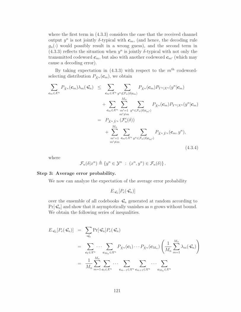
where the first term in (4.3.3) considers the case that the received channeloutput yn is not jointly δ-typical with cm, (and hence, the decoding rulegn(·) would possibly result in a wrong guess), and the second term in(4.3.3) reflects the situation when yn is jointly δ-typical with not only thetransmitted codeword cm, but also with another codeword cm′ (which maycause a decoding error).
By taking expectation in (4.3.3) with respect to the mth codeword-selecting distribution PXn(cm), we obtain
∑
cm∈Xn
PXn(cm)λm( C∼n) ≤∑
cm∈Xn
∑
yn 6∈Fn(δ|cm)
PXn(cm)PY n|Xn(yn|cm)
+∑
cm∈Xn
Mn∑
m′=1m′ 6=m
∑
yn∈Fn(δ|cm′ )
PXn(cm)PY n|Xn(yn|cm)
= PXn,Y n (F cn(δ))
+Mn∑
m′=1m′ 6=m
∑
cm∈Xn
∑
yn∈Fn(δ|cm′ )
PXn,Y n(cm, yn),
(4.3.4)
whereFn(δ|xn) , yn ∈ Yn : (xn, yn) ∈ Fn(δ) .
Step 3: Average error probability.
We now can analyze the expectation of the average error probability
E C∼n [Pe( C∼n)]
over the ensemble of all codebooks C∼n generated at random according toPr[ C∼n] and show that it asymptotically vanishes as n grows without bound.We obtain the following series of inequalities.
E C∼n [Pe( C∼n)] =∑
C∼n
Pr[ C∼n]Pe( C∼n)
=∑
c1∈Xn
· · ·∑
cMn∈Xn
PXn(c1) · · ·PXn(cMn)
(
1
Mn
Mn∑
m=1
λm( C∼n)
)
=1
Mn
Mn∑
m=1
∑
c1∈Xn
· · ·∑
cm−1∈Xn
∑
cm+1∈Xn
· · ·∑
cMn∈Xn
121
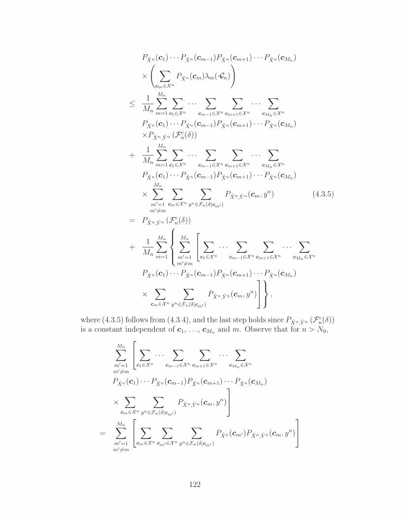
PXn(c1) · · ·PXn(cm−1)PXn(cm+1) · · ·PXn(cMn)
×(∑
cm∈Xn
PXn(cm)λm( C∼n)
)
≤ 1
Mn
Mn∑
m=1
∑
c1∈Xn
· · ·∑
cm−1∈Xn
∑
cm+1∈Xn
· · ·∑
cMn∈Xn
PXn(c1) · · ·PXn(cm−1)PXn(cm+1) · · ·PXn(cMn)
×PXn,Y n (F cn(δ))
+1
Mn
Mn∑
m=1
∑
c1∈Xn
· · ·∑
cm−1∈Xn
∑
cm+1∈Xn
· · ·∑
cMn∈Xn
PXn(c1) · · ·PXn(cm−1)PXn(cm+1) · · ·PXn(cMn)
×Mn∑
m′=1m′ 6=m
∑
cm∈Xn
∑
yn∈Fn(δ|cm′ )
PXn,Y n(cm, yn) (4.3.5)
= PXn,Y n (F cn(δ))
+1
Mn
Mn∑
m=1
Mn∑
m′=1m′ 6=m
∑
c1∈Xn
· · ·∑
cm−1∈Xn
∑
cm+1∈Xn
· · ·∑
cMn∈Xn
PXn(c1) · · ·PXn(cm−1)PXn(cm+1) · · ·PXn(cMn)
×∑
cm∈Xn
∑
yn∈Fn(δ|cm′ )
PXn,Y n(cm, yn)
,
where (4.3.5) follows from (4.3.4), and the last step holds since PXn,Y n (F cn(δ))
is a constant independent of c1, . . ., cMn and m. Observe that for n > N0,
Mn∑
m′=1m′ 6=m
∑
c1∈Xn
· · ·∑
cm−1∈Xn
∑
cm+1∈Xn
· · ·∑
cMn∈Xn
PXn(c1) · · ·PXn(cm−1)PXn(cm+1) · · ·PXn(cMn)
×∑
cm∈Xn
∑
yn∈Fn(δ|cm′ )
PXn,Y n(cm, yn)
=Mn∑
m′=1m′ 6=m
∑
cm∈Xn
∑
cm′∈Xn
∑
yn∈Fn(δ|cm′ )
PXn(cm′)PXn,Y n(cm, yn)
122

=Mn∑
m′=1m′ 6=m
∑
cm′∈Xn
∑
yn∈Fn(δ|cm′ )
PXn(cm′)
(∑
cm∈Xn
PXn,Y n(cm, yn)
)
=Mn∑
m′=1m′ 6=m
∑
cm′∈Xn
∑
yn∈Fn(δ|cm′ )
PXn(cm′)PY n(yn)
=Mn∑
m′=1m′ 6=m
∑
(cm′ ,yn)∈Fn(δ)
PXn(cm′)PY n(yn)
≤Mn∑
m′=1m′ 6=m
|Fn(δ)|2−n(H(X)−δ)2−n(H(Y )−δ)
≤Mn∑
m′=1m′ 6=m
2n(H(X,Y )+δ)2−n(H(X)−δ)2−n(H(Y )−δ)
= (Mn − 1)2n(H(X,Y )+δ)2−n(H(X)−δ)2−n(H(Y )−δ)
< Mn · 2n(H(X,Y )+δ)2−n(H(X)−δ)2−n(H(Y )−δ)
≤ 2n(C−4δ) · 2−n(I(X;Y )−3δ) = 2−nδ,
where the first inequality follows from the definition of the jointly typicalset Fn(δ), the second inequality holds by the Shannon-McMillan theoremfor pairs (Theorem 4.9), the last inequality follows since C = I(X; Y ) bydefinition of X and Y , and since (1/n) log2 Mn ≤ C − (γ/2) = C − 4δ.Consequently,
E C∼n [Pe( C∼n)] ≤ PXn,Y n (F cn(δ)) + 2−nδ,
which for sufficiently large n (and n > N0), can be made smaller than2δ = γ/4 < ε by the Shannon-McMillan theorem for pairs. 2
Before proving the converse part of the channel coding theorem, let us recallFano’s inequality in a channel coding context. Consider an (n,Mn) channelblock code C∼n with encoding and decoding functions given by
fn : 1, 2, · · · ,Mn → X n
andgn : Yn → 1, 2, · · · ,Mn,
123

respectively. Let message W , which is uniformly distributed over the set ofmessages 1, 2, · · · ,Mn, be sent via codeword Xn(W ) = fn(W ) over the DMC,and let Y n be received at the channel output. At the receiver, the decoderestimates the sent message via W = gn(Y n) and the probability of estimationerror is given by the code’s average error probability:
Pr[W 6= W ] = Pe( C∼n)
since W is uniformly distributed. Then Fano’s inequality (2.5.2) yields
H(W |Y n) ≤ 1 + Pe( C∼n) log2(Mn − 1)
< 1 + Pe( C∼n) log2 Mn. (4.3.6)
We next proceed with the proof of the converse part.
Proof of the converse part: For any (n,Mn) block channel code C∼n as de-scribed above, we have that W → Xn → Y n form a Markov chain; we thusobtain by the data processing inequality that
I(W ; Y n) ≤ I(Xn; Y n). (4.3.7)
We can also upper bound I(Xn; Y n) in terms of the channel capacity C as follows
I(Xn; Y n) ≤ maxPXn
I(Xn; Y n)
≤ maxPXn
n∑
i=1
I(Xi; Yi) (by Theorem 2.21)
≤n∑
i=1
maxPXn
I(Xi; Yi)
=n∑
i=1
maxPXi
I(Xi; Yi)
= nC. (4.3.8)
Consequently, code C∼n satisfies the following:
log2 Mn = H(W ) (since W is uniformly distributed)
= H(W |Y n) + I(W ; Y n)
≤ H(W |Y n) + I(Xn; Y n) (by (4.3.7))
≤ H(W |Y n) + nC (by (4.3.8))
< 1 + Pe( C∼n) · log2 Mn + nC. (by (4.3.6))
124

This implies that
Pe( C∼n) > 1 − C
(1/n) log2 Mn
− 1
log2 Mn
= 1 − C + 1/n
(1/n) log2 Mn
.
So if lim infn→∞(1/n) log2 Mn = C1−µ
, then for any 0 < ε < 1, there exists aninteger N such that for n ≥ N ,
1
nlog2 Mn ≥ C + 1/n
1 − (1 − ε)µ, (4.3.9)
because, otherwise, (4.3.9) would be violated for infinitely many n, implying acontradiction that
lim infn→∞
1
nlog2 Mn ≤ lim inf
n→∞
C + 1/n
1 − (1 − ε)µ=
C
1 − (1 − ε)µ.
Hence, for n ≥ N ,
Pe( C∼n) > 1 − [1 − (1 − ε)µ]C + 1/n
C + 1/n= (1 − ǫ)µ > 0;
i.e., Pe( C∼n) is bounded away from zero for n sufficiently large. 2
Observation 4.11 The results of the above channel coding theorem is illus-trated in Figure 4.5,7 where R = lim infn→∞(1/n) log2 Mn (measured in messagebits/channel use) is usually called the ultimate (or asymptotic) coding rate ofchannel block codes. As indicated in the figure, the ultimate rate of any goodblock code for the DMC must be smaller than or equal to the channel capacityC.8 Conversely, any block code with (ultimate) rate greater than C, will haveits probability of error bounded away from zero. Thus for a DMC, its capacityC is the supremum of all “achievable” channel block coding rates; i.e., it is thesupremum of all rates for which there exists a sequence of channel block codeswith asymptotically vanishing (as the blocklength goes to infinity) probabilityof error.
7Note that Theorem 4.10 actually implies that limn→∞ Pe = 0 for R < C and thatlim infn→∞ Pe > 0 for R > C rather than the behavior of lim supn→∞ Pe portrayed in Fig-ure 4.5; these properties however might not hold for more general channels than the DMC.For general channels, three partitions instead of two may result, i.e., R < C, C < R < Cand R > C, which respectively correspond to lim supn→∞ Pe = 0 for the best block code,lim supn→∞ Pe > 0 but lim infn→∞ Pe = 0 for the best block code, and lim infn→∞ Pe > 0for all channel code codes, where C is called the optimistic channel capacity [280, 278]. SinceC = C for DMCs, the three regions are reduced to two. A formula for C in terms of ageneralized (spectral) mutual information rate is established in [51].
8It can be seen from the theorem that C can be achieved as an ultimate transmission rateas long as (1/n) log2 Mn approaches C from below with increasing n (see (4.3.2)).
125
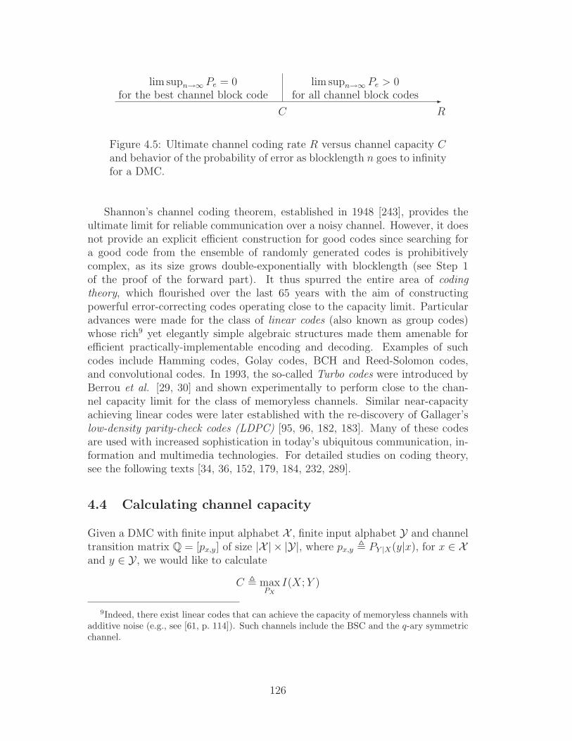
-C
lim supn→∞ Pe = 0for the best channel block code
lim supn→∞ Pe > 0for all channel block codes
R
Figure 4.5: Ultimate channel coding rate R versus channel capacity Cand behavior of the probability of error as blocklength n goes to infinityfor a DMC.
Shannon’s channel coding theorem, established in 1948 [243], provides theultimate limit for reliable communication over a noisy channel. However, it doesnot provide an explicit efficient construction for good codes since searching fora good code from the ensemble of randomly generated codes is prohibitivelycomplex, as its size grows double-exponentially with blocklength (see Step 1of the proof of the forward part). It thus spurred the entire area of codingtheory, which flourished over the last 65 years with the aim of constructingpowerful error-correcting codes operating close to the capacity limit. Particularadvances were made for the class of linear codes (also known as group codes)whose rich9 yet elegantly simple algebraic structures made them amenable forefficient practically-implementable encoding and decoding. Examples of suchcodes include Hamming codes, Golay codes, BCH and Reed-Solomon codes,and convolutional codes. In 1993, the so-called Turbo codes were introduced byBerrou et al. [29, 30] and shown experimentally to perform close to the chan-nel capacity limit for the class of memoryless channels. Similar near-capacityachieving linear codes were later established with the re-discovery of Gallager’slow-density parity-check codes (LDPC) [95, 96, 182, 183]. Many of these codesare used with increased sophistication in today’s ubiquitous communication, in-formation and multimedia technologies. For detailed studies on coding theory,see the following texts [34, 36, 152, 179, 184, 232, 289].
4.4 Calculating channel capacity
Given a DMC with finite input alphabet X , finite input alphabet Y and channeltransition matrix Q = [px,y] of size |X | × |Y|, where px,y , PY |X(y|x), for x ∈ Xand y ∈ Y , we would like to calculate
C , maxPX
I(X; Y )
9Indeed, there exist linear codes that can achieve the capacity of memoryless channels withadditive noise (e.g., see [61, p. 114]). Such channels include the BSC and the q-ary symmetricchannel.
126
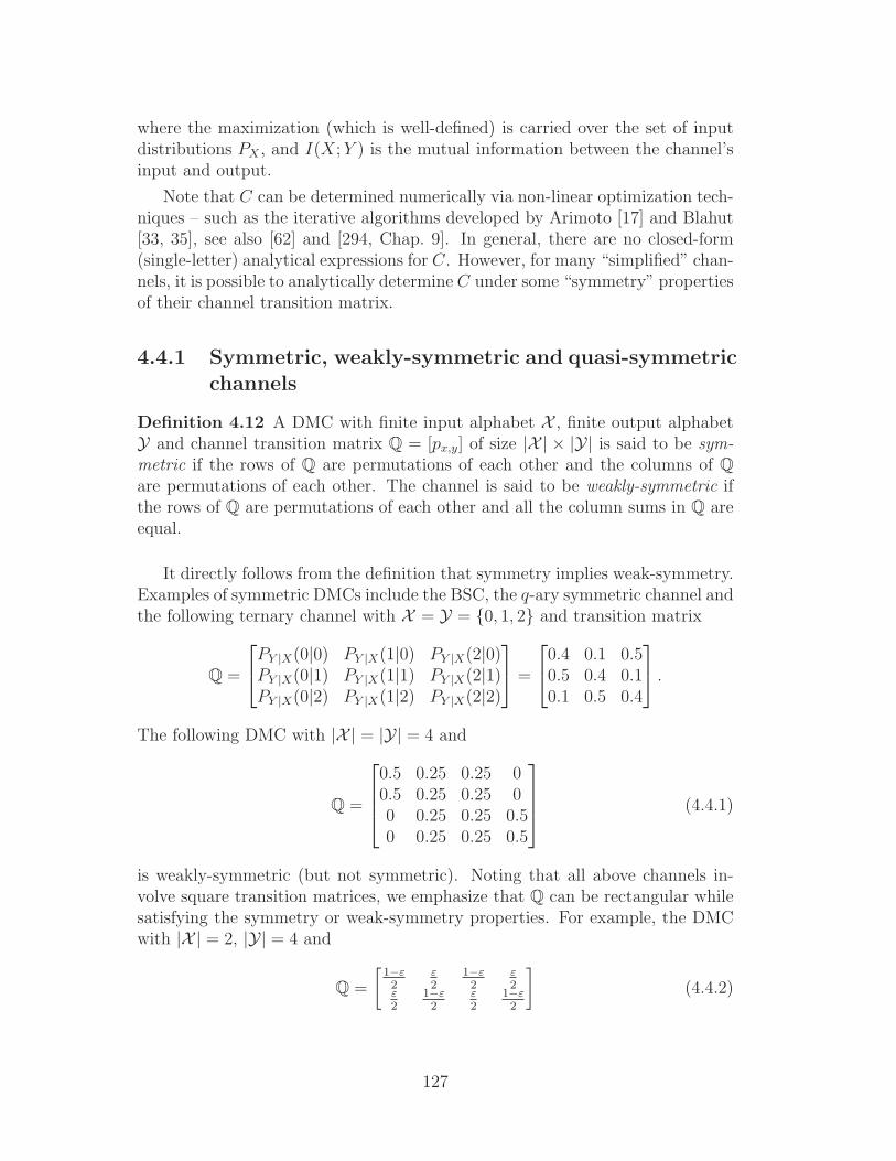
where the maximization (which is well-defined) is carried over the set of inputdistributions PX , and I(X; Y ) is the mutual information between the channel’sinput and output.
Note that C can be determined numerically via non-linear optimization tech-niques – such as the iterative algorithms developed by Arimoto [17] and Blahut[33, 35], see also [62] and [294, Chap. 9]. In general, there are no closed-form(single-letter) analytical expressions for C. However, for many “simplified” chan-nels, it is possible to analytically determine C under some “symmetry” propertiesof their channel transition matrix.
4.4.1 Symmetric, weakly-symmetric and quasi-symmetricchannels
Definition 4.12 A DMC with finite input alphabet X , finite output alphabetY and channel transition matrix Q = [px,y] of size |X | × |Y| is said to be sym-metric if the rows of Q are permutations of each other and the columns of Q
are permutations of each other. The channel is said to be weakly-symmetric ifthe rows of Q are permutations of each other and all the column sums in Q areequal.
It directly follows from the definition that symmetry implies weak-symmetry.Examples of symmetric DMCs include the BSC, the q-ary symmetric channel andthe following ternary channel with X = Y = 0, 1, 2 and transition matrix
Q =
PY |X(0|0) PY |X(1|0) PY |X(2|0)PY |X(0|1) PY |X(1|1) PY |X(2|1)PY |X(0|2) PY |X(1|2) PY |X(2|2)
=
0.4 0.1 0.50.5 0.4 0.10.1 0.5 0.4
.
The following DMC with |X | = |Y| = 4 and
Q =
0.5 0.25 0.25 00.5 0.25 0.25 00 0.25 0.25 0.50 0.25 0.25 0.5
(4.4.1)
is weakly-symmetric (but not symmetric). Noting that all above channels in-volve square transition matrices, we emphasize that Q can be rectangular whilesatisfying the symmetry or weak-symmetry properties. For example, the DMCwith |X | = 2, |Y| = 4 and
Q =
[1−ε2
ε2
1−ε2
ε2
ε2
1−ε2
ε2
1−ε2
]
(4.4.2)
127
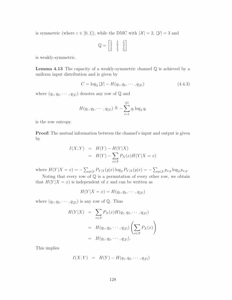
is symmetric (where ε ∈ [0, 1]), while the DMC with |X | = 2, |Y| = 3 and
Q =
[13
16
12
13
12
16
]
is weakly-symmetric.
Lemma 4.13 The capacity of a weakly-symmetric channel Q is achieved by auniform input distribution and is given by
C = log2 |Y| − H(q1, q2, · · · , q|Y|) (4.4.3)
where (q1, q2, · · · , q|Y|) denotes any row of Q and
H(q1, q2, · · · , q|Y|) , −|Y|∑
i=1
qi log2 qi
is the row entropy.
Proof: The mutual information between the channel’s input and output is givenby
I(X; Y ) = H(Y ) − H(Y |X)
= H(Y ) −∑
x∈XPX(x)H(Y |X = x)
where H(Y |X = x) = −∑y∈Y PY |X(y|x) log2 PY |X(y|x) = −∑y∈Y px,y log2 px,y.
Noting that every row of Q is a permutation of every other row, we obtainthat H(Y |X = x) is independent of x and can be written as
H(Y |X = x) = H(q1, q2, · · · , q|Y|)
where (q1, q2, · · · , q|Y|) is any row of Q. Thus
H(Y |X) =∑
x∈XPX(x)H(q1, q2, · · · , q|Y|)
= H(q1, q2, · · · , q|Y|)
(∑
x∈XPX(x)
)
= H(q1, q2, · · · , q|Y|).
This implies
I(X; Y ) = H(Y ) − H(q1, q2, · · · , q|Y|)
128

≤ log2 |Y| − H(q1, q2, · · · , q|Y|)
with equality achieved iff Y is uniformly distributed over Y . We next show thatchoosing a uniform input distribution, PX(x) = 1
|X | ∀x ∈ X , yields a uniformoutput distribution, hence maximizing mutual information. Indeed, under auniform input distribution, we obtain that for any y ∈ Y ,
PY (y) =∑
x∈XPX(x)PY |X(y|x) =
1
|X |∑
x∈Xpx,y =
A
|X |
where A ,∑
x∈X px,y is a constant given by the sum of the entries in any columnof Q, since by the weak-symmetry property all column sums in Q are identical.Note that
∑
y∈Y PY (y) = 1 yields that
∑
y∈Y
A
|X | = 1
and hence
A =|X ||Y| . (4.4.4)
Accordingly,
PY (y) =A
|X | =|X ||Y|
1
|X | =1
|Y|for any y ∈ Y ; thus the uniform input distribution induces a uniform outputdistribution and achieves channel capacity as given by (4.4.3). 2
Observation 4.14 Note that if the weakly-symmetric channel has a square (i.e.,with |X | = |Y|) transition matrix Q, then Q is a doubly-stochastic matrix; i.e.,both its row sums and its column sums are equal to 1. Note however that havinga square transition matrix does not necessarily make a weakly-symmetric channelsymmetric; e.g., see (4.4.1).
Example 4.15 (Capacity of the BSC) Since the BSC with crossover proba-bility (or bit error rate) ε is symmetric, we directly obtain from Lemma 4.13that its capacity is achieved by a uniform input distribution and is given by
C = log2(2) − H(1 − ε, ε) = 1 − hb(ε) (4.4.5)
where hb(·) is the binary entropy function.
129
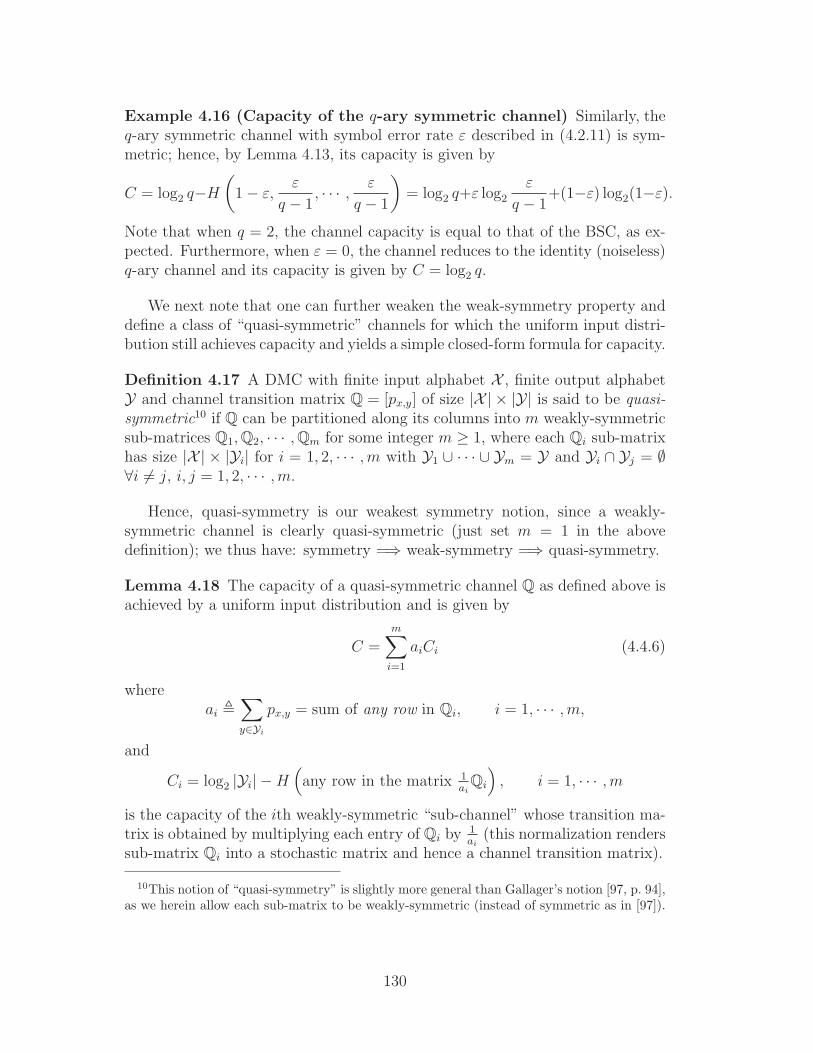
Example 4.16 (Capacity of the q-ary symmetric channel) Similarly, theq-ary symmetric channel with symbol error rate ε described in (4.2.11) is sym-metric; hence, by Lemma 4.13, its capacity is given by
C = log2 q−H
(
1 − ε,ε
q − 1, · · · ,
ε
q − 1
)
= log2 q+ε log2
ε
q − 1+(1−ε) log2(1−ε).
Note that when q = 2, the channel capacity is equal to that of the BSC, as ex-pected. Furthermore, when ε = 0, the channel reduces to the identity (noiseless)q-ary channel and its capacity is given by C = log2 q.
We next note that one can further weaken the weak-symmetry property anddefine a class of “quasi-symmetric” channels for which the uniform input distri-bution still achieves capacity and yields a simple closed-form formula for capacity.
Definition 4.17 A DMC with finite input alphabet X , finite output alphabetY and channel transition matrix Q = [px,y] of size |X | × |Y| is said to be quasi-symmetric10 if Q can be partitioned along its columns into m weakly-symmetricsub-matrices Q1, Q2, · · · , Qm for some integer m ≥ 1, where each Qi sub-matrixhas size |X | × |Yi| for i = 1, 2, · · · ,m with Y1 ∪ · · · ∪ Ym = Y and Yi ∩ Yj = ∅∀i 6= j, i, j = 1, 2, · · · ,m.
Hence, quasi-symmetry is our weakest symmetry notion, since a weakly-symmetric channel is clearly quasi-symmetric (just set m = 1 in the abovedefinition); we thus have: symmetry =⇒ weak-symmetry =⇒ quasi-symmetry.
Lemma 4.18 The capacity of a quasi-symmetric channel Q as defined above isachieved by a uniform input distribution and is given by
C =m∑
i=1
aiCi (4.4.6)
whereai ,
∑
y∈Yi
px,y = sum of any row in Qi, i = 1, · · · ,m,
and
Ci = log2 |Yi| − H(
any row in the matrix 1ai
Qi
)
, i = 1, · · · ,m
is the capacity of the ith weakly-symmetric “sub-channel” whose transition ma-trix is obtained by multiplying each entry of Qi by 1
ai(this normalization renders
sub-matrix Qi into a stochastic matrix and hence a channel transition matrix).
10This notion of “quasi-symmetry” is slightly more general than Gallager’s notion [97, p. 94],as we herein allow each sub-matrix to be weakly-symmetric (instead of symmetric as in [97]).
130

Proof: We first observe that for each i = 1, · · · ,m, ai is independent of theinput value x, since sub-matrix i is weakly-symmetric (so any row in Qi is apermutation of any other row); and hence ai is the sum of any row in Qi.
For each i = 1, · · · ,m, define
PYi|X(y|x) ,
px,y
aiif y ∈ Yi and x ∈ X ;
0 otherwise
where Yi is a random variable taking values in Yi. It can be easily verified thatPYi|X(y|x) is a legitimate conditional distribution. Thus [PYi|X(y|x)] = 1
aiQi
is the transition matrix of the weakly-symmetric “sub-channel” i with inputalphabet X and output alphabet Yi. Let I(X; Yi) denote its mutual information.Since each such sub-channel i is weakly-symmetric, we know that its capacityCi is given by
Ci = maxPX
I(X; Yi) = log2 |Yi| − H(
any row in the matrix 1ai
Qi
)
,
where the maximum is achieved by a uniform input distribution.
Now, the mutual information between the input and the output of our originalquasi-symmetric channel Q can be written as
I(X; Y ) =∑
y∈Y
∑
x∈XPX(x) px,y log2
px,y∑
x′∈X PX(x′)px′,y
=m∑
i=1
∑
y∈Yi
∑
x∈Xai PX(x)
px,y
ai
log2
px,y
ai∑
x′∈X PX(x′)px′,y
ai
=m∑
i=1
ai
∑
y∈Yi
∑
x∈XPX(x)PYi|X(y|x) log2
PYi|X(y|x)∑
x′∈X PX(x′)PYi|X(y|x′)
=m∑
i=1
ai I(X; Yi).
Therefore, the capacity of channel Q is
C = maxPX
I(X; Y )
= maxPX
m∑
i=1
ai I(X; Yi)
=m∑
i=1
ai maxPX
I(X; Yi) (as the same uniform PX maximizes each I(X; Yi))
=m∑
i=1
ai Ci.
2
131

Example 4.19 (Capacity of the BEC) The BEC with erasure probability αas given in (4.2.6) is quasi-symmetric (but neither weakly-symmetric nor sym-metric). Indeed, its transition matrix Q can be partitioned along its columnsinto two symmetric (hence weakly-symmetric) sub-matrices
Q1 =
[1 − α 0
0 1 − α
]
and
Q2 =
[αα
]
.
Thus applying the capacity formula for quasi-symmetric channels of Lemma 4.18yields that the capacity of the BEC is given by
C = a1C1 + a2C2
where a1 = 1 − α, a2 = α,
C1 = log2(2) − H
(1 − α
1 − α,
0
1 − α
)
= 1 − H(1, 0) = 1 − 0 = 1,
andC2 = log2(1) − H
(α
α
)
= 0 − 0 = 0.
Therefore, the BEC capacity is given by
C = (1 − α)(1) + (α)(0) = 1 − α. (4.4.7)
Example 4.20 (Capacity of the BSEC) Similarly, the BSEC with crossoverprobability ε and erasure probability α as described in (4.2.8) is quasi-symmetric;its transition matrix can be partitioned along its columns into two symmetricsub-matrices
Q1 =
[1 − ε − α ε
ε 1 − ε − α
]
and
Q2 =
[αα
]
.
Hence by Lemma 4.18, the channel capacity is given by C = a1C1 + a2C2 wherea1 = 1 − α, a2 = α,
C1 = log2(2) − H
(1 − ε − α
1 − α,
ε
1 − α
)
= 1 − hb
(1 − ε − α
1 − α
)
,
andC2 = log2(1) − H
(α
α
)
= 0.
132

We thus obtain that
C = (1 − α)
[
1 − hb
(1 − ε − α
1 − α
)]
+ (α)(0)
= (1 − α)
[
1 − hb
(1 − ε − α
1 − α
)]
. (4.4.8)
As already noted, the BSEC is a combination of the BSC with bit error rate εand the BEC with erasure probability α. Indeed, setting α = 0 in (4.4.8) yieldsthat C = 1 − hb(1 − ε) = 1 − hb(ε) which is the BSC capacity. Furthermore,setting ε = 0 results in C = 1 − α, the BEC capacity.
4.4.2 Karuch-Kuhn-Tucker condition for channel capac-ity
When the channel does not satisfy any symmetry property, the following neces-sary and sufficient Karuch-Kuhn-Tucker (KKT) condition (e.g., cf. Appendix B.10,[97, pp. 87-91] or [31, 38]) for calculating channel capacity can be quite useful.
Definition 4.21 (Mutual information for a specific input symbol) Themutual information for a specific input symbol is defined as:
I(x; Y ) ,∑
y∈YPY |X(y|x) log2
PY |X(y|x)
PY (y).
From the above definition, the mutual information becomes:
I(X; Y ) =∑
x∈XPX(x)
∑
y∈YPY |X(y|x) log2
PY |X(y|x)
PY (y)
=∑
x∈XPX(x)I(x; Y ).
Lemma 4.22 (KKT condition for channel capacity) For a given DMC, aninput distribution PX achieves its channel capacity iff there exists a constant Csuch that
I(x : Y ) = C ∀x ∈ X with PX(x) > 0;
I(x : Y ) ≤ C ∀x ∈ X with PX(x) = 0.(4.4.9)
Furthermore, the constant C is the channel capacity (justifying the choice ofnotation).
133

Proof: The forward (if) part holds directly; hence, we only prove the converse(only-if) part. Without loss of generality, we assume that PX(x) < 1 for allx ∈ X , since PX(x) = 1 for some x implies that I(X; Y ) = 0. The problem ofcalculating the channel capacity is to maximize
I(X; Y ) =∑
x∈X
∑
y∈YPX(x)PY |X(y|x) log2
PY |X(y|x)∑
x′∈X PX(x′)PY |X(y|x′), (4.4.10)
subject to the condition∑
x∈XPX(x) = 1 (4.4.11)
for a given channel distribution PY |X . By using the Lagrange multiplier method(e.g., see Appendix B.10 or [31]), maximizing (4.4.10) subject to (4.4.11) isequivalent to maximize:
f(PX) ,∑
x∈Xy∈Y
PX(x)PY |X(y|x) log2
PY |X(y|x)∑
x′∈XPX(x′)PY |X(y|x′)
+ λ
(∑
x∈XPX(x) − 1
)
.
We then take the derivative of the above quantity with respect to PX(x′′), andobtain that11
∂f(PX)
∂PX(x′′)= I(x′′; Y ) − log2(e) + λ.
11The details for taking the derivative are as follows:
∂
∂PX(x′′)
∑
x∈X
∑
y∈Y
PX(x)PY |X(y|x) log2 PY |X(y|x)
−∑
x∈X
∑
y∈Y
PX(x)PY |X(y|x) log2
[∑
x′∈X
PX(x′)PY |X(y|x′)
]
+ λ
(∑
x∈X
PX(x) − 1
)
=∑
y∈Y
PY |X(y|x′′) log2 PY |X(y|x′′) −
∑
y∈Y
PY |X(y|x′′) log2
[∑
x′∈X
PX(x′)PY |X(y|x′)
]
+ log2(e)∑
x∈X
∑
y∈Y
PX(x)PY |X(y|x)PY |X(y|x′′)
∑
x′∈X PX(x′)PY |X(y|x′)
+ λ
= I(x′′;Y ) − log2(e)∑
y∈Y
[∑
x∈X
PX(x)PY |X(y|x)
]
PY |X(y|x′′)∑
x′∈X PX(x′)PY |X(y|x′)+ λ
= I(x′′;Y ) − log2(e)∑
y∈Y
PY |X(y|x′′) + λ
= I(x′′;Y ) − log2(e) + λ.
134

By Property 2 of Lemma 2.46, I(X; Y ) = I(PX , PY |X) is a concave function inPX (for a fixed PY |X). Therefore, the maximum of I(PX , PY |X) occurs for a zeroderivative when PX(x) does not lie on the boundary, namely 1 > PX(x) > 0.For those PX(x) lying on the boundary, i.e., PX(x) = 0, the maximum occurs iffa displacement from the boundary to the interior decreases the quantity, whichimplies a non-positive derivative, namely
I(x; Y ) ≤ −λ + log2(e), for those x with PX(x) = 0.
To summarize, if an input distribution PX achieves the channel capacity, then
I(x′′; Y ) = −λ + log2(e), for PX(x′′) > 0;I(x′′; Y ) ≤ −λ + log2(e), for PX(x′′) = 0.
for some λ. With the above result, setting C = −λ + 1 yields (4.4.9). Finally,multiplying both sides of each equation in (4.4.9) by PX(x) and summing overx yields that maxPX
I(X; Y ) on the left and the constant C on the right, thusproving that the constant C is indeed the channel’s capacity. 2
Example 4.23 (Quasi-symmetric channels) For a quasi-symmetric channel,one can directly verify that the uniform input distribution satisfies the KKT con-dition of Lemma 4.22 and yields that the channel capacity is given by (4.4.6);this is left as an exercise. As we already saw, the BSC, the q-ary symmetricchannel, the BEC and the BSEC are all quasi-symmetric.
Example 4.24 Consider a DMC with a ternary input alphabet X = 0, 1, 2,binary output alphabet Y = 0, 1 and the following transition matrix
Q =
1 012
12
0 1
.
This channel is not quasi-symmetric. However, one may guess that the capacityof this channel is achieved by the input distribution (PX(0), PX(1), PX(2)) =(1
2, 0, 1
2) since the input x = 1 has an equal conditional probability of being re-
ceived as 0 or 1 at the output. Under this input distribution, we obtain thatI(x = 0; Y ) = I(x = 2; Y ) = 1 and that I(x = 1; Y ) = 0. Thus the KKT con-dition of (4.4.9) is satisfied; hence confirming that the above input distributionachieves channel capacity and that channel capacity is equal to 1 bit.
Observation 4.25 (Capacity achieved by a uniform input distribution)We close this section by noting that there is a class of DMCs that is largerthan that of quasi-symmetric channels for which the uniform input distribution
135

achieves capacity. It concerns the class of so-called “T -symmetric” channels [230,Section V, Definition 1] for which
T (x) , I(x; Y ) − log2 |X | =∑
y∈YPY |X(y|x) log2
PY |X(y|x)∑
x′∈X PY |X(y|x′)
is a constant function of x (i.e., independent of x), where I(x; Y ) is the mu-tual information for input x under a uniform input distribution. Indeed theT -symmetry condition is equivalent to the property of having the uniform inputdistribution achieve capacity. This directly follows from the KKT condition ofLemma 4.22. An example of a T -symmetric channel that is not quasi-symmetricis the binary-input ternary-output channel with the following transition matrix
Q =
[13
13
13
16
16
23
]
.
Hence its capacity is achieved by the uniform input distribution. See [230, Fig-ure 2] for (infinitely-many) other examples of T -symmetric channels. However,unlike quasi-symmetric channels, T -symmetric channels do not admit in gen-eral a simple closed-form expression for their capacity (such as the one given in(4.4.6)).
4.5 Lossless joint source-channel coding and Shannon’sseparation principle
We next establish Shannon’s lossless joint source-channel coding theorem12 whichprovides explicit (and directly verifiable) conditions for any communication sys-tem in terms of its source and channel information-theoretic quantities underwhich the source can be reliably transmitted (i.e., with asymptotically vanishingerror probability). More specifically, this theorem consists of two parts: (i) aforward part which reveals that if the minimal achievable compression (or sourcecoding) rate of a source is strictly smaller than the capacity of a channel, thenthe source can be reliably sent over the channel via rate-one source-channel blockcodes; (ii) a converse part which states that if the source’s minimal achievablecompression rate is strictly larger than the channel capacity, then the source can-not be reliably sent over the channel via rate-one source-channel block codes. Thetheorem (under minor modifications) has also a more general version in terms ofreliable transmissibility of the source over the channel via source-channel blockcodes of arbitrary rate (not necessarily equal to one).
12This theorem is sometimes referred to as the lossless information transmission theorem.
136

This key theorem is usually referred to as Shannon’s source-channel sepa-ration theorem or principle; this renaming is explained in the following. First,the theorem’s necessary and sufficient conditions for reliable transmissibility area function of entirely “separable” or “disentangled” information quantities, thesource’s minimal compression rate and the channel’s capacity with no quantitiesthat depends on both the source and the channel; this can be seen as a “func-tional separation” property or condition. Second, the proof of the forward part,which (as we will see) consists of properly combining Shannon’s source coding(Theorems 3.5 or 3.14) and channel coding (Theorem 4.10) theorems, showsthat reliable transmissibility can be realized by separating (or decomposing) thesource-channel coding function into two distinct and independently conceivedsource and channel coding operations applied in tandem, where the source codedepends only on the source statistics and, similarly, the channel code is a solefunction of the channel statistics. In other words, we have “operational separa-tion”in that a separate (tandem or two-stage) source and channel coding schemeas depicted in Figure 4.6 is as good (in terms of asymptotic reliable transmissibil-ity) as the more general joint source-channel coding scheme shown in Figure 4.7in which the coding operation can include a combined (one-stage) code designedwith respect to both the source and the channel or jointly coordinated sourceand channel codes. Now, gathering the above two facts with the theorem’s con-verse part – with the exception of the unresolved case where the source’s minimalachievable compression rate is exactly equal to the channel capacity – impliesthat either reliable transmissibility of the source over the channel is achievablevia separate source and channel coding (under the transmissibility condition) orit is not at all achievable, hence justifying calling the theorem by the separationprinciple.
We will prove the theorem by assuming that the source is stationary ergodic13
in the forward part and just stationary in the converse part and that the channelis a DMC; note that the theorem can be extended to more general sources andchannels with memory (see [67, 278, 51]).
Source - SourceEncoder
- ChannelEncoder
-Xn
Channel -Y nChannelDecoder
- SourceDecoder
- Sink
Figure 4.6: A separate (tandem) source-channel coding scheme.
Definition 4.26 (Source-channel block code) Given a discrete source Vi∞i=1
with finite alphabet V and a discrete channel PY n|Xn∞n=1 with finite input
13The minimal achievable compression rate of such sources is given by the entropy rate, seeTheorem 3.14.
137
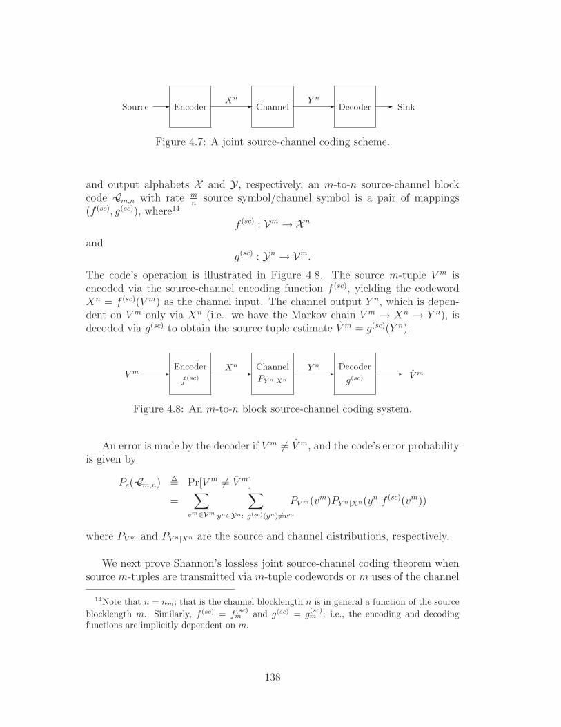
Source - Encoder -Xn
Channel -Y n
Decoder - Sink
Figure 4.7: A joint source-channel coding scheme.
and output alphabets X and Y , respectively, an m-to-n source-channel blockcode C∼m,n with rate m
nsource symbol/channel symbol is a pair of mappings
(f (sc), g(sc)), where14
f (sc) : Vm → X n
andg(sc) : Yn → Vm.
The code’s operation is illustrated in Figure 4.8. The source m-tuple V m isencoded via the source-channel encoding function f (sc), yielding the codewordXn = f (sc)(V m) as the channel input. The channel output Y n, which is depen-dent on V m only via Xn (i.e., we have the Markov chain V m → Xn → Y n), isdecoded via g(sc) to obtain the source tuple estimate V m = g(sc)(Y n).
V m - Encoder
f (sc)-Xn Channel
PY n|Xn
-Y n Decoder
g(sc)- V m
Figure 4.8: An m-to-n block source-channel coding system.
An error is made by the decoder if V m 6= V m, and the code’s error probabilityis given by
Pe( C∼m,n) , Pr[V m 6= V m]
=∑
vm∈Vm
∑
yn∈Yn: g(sc)(yn) 6=vm
PV m(vm)PY n|Xn(yn|f (sc)(vm))
where PV m and PY n|Xn are the source and channel distributions, respectively.
We next prove Shannon’s lossless joint source-channel coding theorem whensource m-tuples are transmitted via m-tuple codewords or m uses of the channel
14Note that n = nm; that is the channel blocklength n is in general a function of the source
blocklength m. Similarly, f (sc) = f(sc)m and g(sc) = g
(sc)m ; i.e., the encoding and decoding
functions are implicitly dependent on m.
138

(i.e., when n = m or for rate-one source-channel block codes). The source isassumed to have memory (as indicated below), while the channel is memoryless.
Theorem 4.27 (Lossless joint source-channel coding theorem for rate-one block codes) Consider a discrete source Vi∞i=1 with finite alphabet V andentropy rate15 H(V) and a DMC with input alphabet X , output alphabet Y andcapacity C, where both H(V) and C are measured in the same units (i.e., theyboth use the same base of the logarithm). Then the following hold:
• Forward part (achievability): For any 0 < ǫ < 1 and given that the sourceis stationary ergodic, if
H(V) < C,
then there exists a sequence of rate-one source-channel codes C∼m,m∞m=1
such thatPe( C∼m,m) < ǫ for sufficiently large m,
where Pe( C∼m,m) is the error probability of the source-channel code C∼m,m.
• Converse part: For any 0 < ǫ < 1 and given that the source is stationary,if
H(V) > C,
then any sequence of rate-one source-channel codes C∼m,m∞m=1 satisfies
Pe( C∼m,m) > (1 − ǫ)µ for sufficiently large m, (4.5.1)
where µ = HD(V) − CD with D = |V|, and HD(V) and CD are entropyrate and channel capacity measured in D-ary digits, i.e., the codes’ errorprobability is bounded away from zero and it is not possible to transmitthe source over the channel via rate-one source-channel block codes witharbitrarily low error probability.16
Proof of the forward part: Without loss of generality, we assume throughoutthis proof that both the source entropy rate H(V) and the channel capacity Care measured in nats (i.e., they are both expressed using the natural logarithm).
We will show the existence of the desired rate-one source-channel codes C∼m,m
via a separate (tandem or two-stage) source and channel coding scheme as theone depicted in Figure 4.6.
15We assume the source entropy rate exists as specified below.
16Note that (4.5.1) actually implies that lim infm→∞ Pe( C∼m,m) ≥ limǫ↓0(1− ǫ)µ = µ, wherethe error probability lower bound has nothing to do with ǫ. Here we state the converse ofTheorem 4.27 in a form in parallel to the converse statements in Theorems 3.5, 3.14 and 4.10.
139

Let γ , C − H(V) > 0. Now, given any 0 < ǫ < 1, by the lossless source-coding theorem for stationary ergodic sources (Theorem 3.14), there exists asequence of source codes of blocklength m and size Mm with encoder
fs : Vm → 1, 2, · · · ,Mmand decoder
gs : 1, 2, · · · ,Mm → Vm
such that1
mlog Mm < H(V) + γ/2 (4.5.2)
andPr [gs(fs(V
m)) 6= V m] < ǫ/2
for m sufficiently large.17
Furthermore, by the channel coding theorem under the maximal probabilityof error criterion (see Observation 4.6 and Theorem 4.10), there exists a sequenceof channel codes of blocklength m and size Mm with encoder
fc : 1, 2, · · · , Mm → Xm
and decodergc : Ym → 1, 2, · · · , Mm
such that18
1
mlog Mm > C − γ/2
(= H(V) + γ/2 >
1
mlog Mm
)(4.5.5)
17Theorem 3.14 indicates that for any 0 < ε′ , minε/2, γ/(2 log(2)) < 1, there exists δwith 0 < δ < ε′ and a sequence of binary block codes C∼m = (m,Mm)∞m=1 with
lim supm→∞
1
mlog2 Mm < H2(V) + δ, (4.5.3)
and probability of decoding error satisfying Pe( C∼m) < ε′ (≤ ε/2) for sufficiently large m, whereH2(V) is the entropy rate measured in bits. Here (4.5.3) implies that 1
m log2 Mm < H2(V) + δfor sufficiently large m. Hence,
1
mlog Mm < H(V) + δ log(2) < H(V) + ε′ log(2) ≤ H(V) + γ/2
for sufficiently large m.
18Theorem 4.10 and its proof of forward part indicate that for any 0 < ε′ ,
minε/4, γ/(16 log(2)) < 1, there exist 0 < γ′ < min4ε′, C2 = minε, γ/(4 log(2)), C2and a sequence of data transmission block codes C∼′
m = (m, M ′m)∞m=1 satisfying
C2 − γ′ <1
mlog2 M ′
m ≤ C2 −γ′
2(4.5.4)
andPe( C∼′
m) < ε′ for sufficiently large m,
140

andλ , max
w∈1,··· ,MmPr [gc(Y
m) 6= w|Xm = fc(w)] < ǫ/2
for m sufficiently large.
Now we form our source-channel code by concatenating in tandem the abovesource and channel codes. Specifically, the m-to-m source-channel code C∼m,m
has the following encoder-decoder pair (f (sc), g(sc)):
f (sc) : Vm → Xm with f (sc)(vm) = fc(fs(vm)) ∀vm ∈ Vm
andg(sc) : Ym → Vm
with
g(sc)(ym) =
gs(gc(ym)), if gc(y
m) ∈ 1, 2, . . . ,Mmarbitrary, otherwise
∀ym ∈ Ym.
The above construction is possible since 1, 2, . . . ,Mm is a subset of 1, 2, . . .,Mm. The source-channel code’s error probability can be analyzed by consideringthe cases of whether or not a channel decoding error occurs as follows:
Pe( C∼m,m) = Pr[g(sc)(Y m) 6= V m]
= Pr[g(sc)(Y m) 6= V m ∧ gc(Ym) = fs(V
m)]
+ Pr[g(sc)(Y m) 6= V m ∧ gc(Ym) 6= fs(V
m)]
= Pr[gs(gc(Ym)) 6= V m ∧ gc(Y
m) = fs(Vm)]
+ Pr[g(sc)(Y m) 6= V m ∧ gc(Ym) 6= fs(V
m)]
≤ Pr[gs(fs(Vm)) 6= V m] + Pr[gc(Y
m) 6= fs(Vm)]
= Pr[gs(fs(Vm)) 6= V m]
+∑
w∈1,2,...,MmPr[fs(V
m) = w] Pr[gc(Ym) 6= w|fs(V
m) = w]
= Pr[gs(fs(Vm)) 6= V m]
provided that C2 > 0, where C2 is the channel capacity measured in bits.Observation 4.6 indicates that by throwing away from C∼′
m half of its codewords with largestconditional probability of error, a new code C∼m = (m, Mm) = (m, M ′
m/2) is obtained, whichsatisfies λ( C∼m) ≤ 2Pe( C∼′
m) < 2ε′ ≤ ε/2.(4.5.4) then implies that for m > 1/γ′ sufficiently large,
1
mlog Mm =
1
mlog M ′
m − 1
mlog(2) > C − γ′ log(2) − 1
mlog(2) > C − 2γ′ log(2) > C − γ/2.
141

+∑
w∈1,2,...,MmPr[Xm = fc(w)] Pr[gc(Y
m) 6= w|Xm = fc(w)]
≤ Pr[gs(fs(Vm)) 6= V m] + λ
< ǫ/2 + ǫ/2 = ǫ
for m sufficiently large. Thus the source can be reliably sent over the channelvia rate-one block source-channel codes as long as H(V) < C. 2
Proof of the converse part: For simplicity, we assume in this proof that H(V)and C are measured in bits.
For any m-to-m source-channel code C∼m,m, we can write
H(V) ≤ 1
mH(V m) (4.5.6)
=1
mH(V m|V m) +
1
mI(V m; V m)
≤ 1
m[Pe( C∼m,m) log2(|V|m) + 1] +
1
mI(V m; V m) (4.5.7)
≤ Pe( C∼m,m) log2 |V| +1
m+
1
mI(Xm; Y m) (4.5.8)
≤ Pe( C∼m,m) log2 |V| +1
m+ C (4.5.9)
where
• (4.5.6) is due to the fact that (1/m)H(V m) is non-increasing in m andconverges to H(V) as m → ∞ since the source is stationary (see Observa-tion 3.11),
• (4.5.7) follows from Fano’s inequality,
H(V m|V m) ≤ Pe( C∼m,m) log2(|V|m)+hb(Pe( C∼m,m)) ≤ Pe( C∼m,m) log2(|V|m)+1,
• (4.5.8) is due to the data processing inequality since V m → Xm → Y m →V m form a Markov chain,
• and (4.5.9) holds by (4.3.8) since the channel is a DMC.
Note that in the above derivation, the information measures are all measured inbits. This implies that for m ≥ logD(2)/(εµ),
Pe( C∼m,m) ≥ H(V) − C
log2(|V|)− 1
m log2(|V|)= HD(V) − CD − logD(2)
m≥ (1 − ε)µ.
2
142

Observation 4.28 We make the following remarks regarding the above jointsource-channel coding theorem:
• In general, it is not known whether the source can be (asymptotically)reliably transmitted over the DMC when
H(V) = C
even if the source is a DMS. This is because separate source and channelcoding is used to prove the forward part of the theorem and the factsthat the source coding rate approaches the source entropy rate from above(cf. (4.5.2)) while the channel coding rate approaches channel capacityfrom below (cf. (4.5.5)).
• The above theorem directly holds for DMSs since any DMS is stationaryand ergodic.
• We can expand the forward part of the theorem above by replacing therequirement that the source be stationary ergodic with the more generalcondition that the source be information stable.19 Note that time-invariantirreducible Markov sources (that are not necessarily stationary) are infor-mation stable.
The above lossless joint source-channel coding theorem can be readily gen-eralized for m-to-n source-channel codes – i.e., codes with rate not necessarilyequal to one – as follows (its proof, which is similar to the previous theorem, isleft as an exercise).
Theorem 4.29 (Lossless joint source-channel coding theorem for gen-eral rate block codes) Consider a discrete source Vi∞i=1 with finite alphabetV and entropy rate H(V) and a DMC with input alphabet X , output alphabetY and capacity C, where both H(V) and C are measured in the same units.Then the following hold:
• Forward part (achievability): For any 0 < ǫ < 1 and given that the sourceis stationary ergodic, there exists a sequence of m-to-nm source-channelcodes C∼m,nm∞m=1 such that
Pe( C∼m,nm) < ǫ for sufficiently large m
if
lim supm→∞
m
nm
<C
H(V).
19See [67, 214, 278, 51] for a definition of information stable sources, whose property isslightly more general than the Generalized AEP property given in Theorem 3.13.
143

• Converse part: For any 0 < ǫ < 1 and given that the source is stationary,any sequence of m-to-nm source-channel codes C∼m,nm∞m=1 with
lim infm→∞
m
nm
>C
H(V),
satisfiesPe( C∼m,nm) > (1 − ǫ)µ for sufficiently large m,
for some positive constant µ that depends on lim infm→∞(m/nm), H(V)and C, i.e., the codes’ error probability is bounded away from zero andit is not possible to transmit the source over the channel via m-to-nm
source-channel block codes with arbitrarily low error probability.
Discussion: separate vs joint source-channel coding
Shannon’s separation principle has provided the linchpin for most modern com-munication systems where source coding and channel coding schemes are sep-arately constructed (with the source (resp., channel) code designed by onlytaking into account the source (resp., channel) characteristics) and applied intandem without the risk of sacrificing optimality in terms of reliable transmis-sibility under unlimited coding delay and complexity. This result is the rai-son d’etre for separately studying the practices of source coding or data com-pression (e.g., see [27, 104, 117, 204, 236, 237]) and channel coding (e.g., see[184, 289, 152, 179, 232]). Furthermore, by disentangling the source and channelcoding operations, separate coding offers appealing properties such as systemmodularity and flexibility. For example, if one needs to send different sourcesover the same channel, using the separate coding approach, one only needs tomodify the source code while keeping the channel code unchanged (analogously,if a single source is to be communicated over different channels, one only has toadapt the channel code).
However, in practical implementations, there is a price to pay in delay andcomplexity for extremely long coding blocklengths (particularly when delay andcomplexity constraints are quite stringent such as in wireless communicationssystems). To begin, note that joint source-channel coding might be expected tooffer improvements for the combination of a source with significant redundancyand a channel with significant noise, since, for such a system, separate codingwould involve source coding to remove redundancy followed by channel codingto insert redundancy. It is a natural conjecture that this is not the most efficientapproach even if the blocklength is allowed to grow without bound. Indeed,Shannon [243] made this point as follows:
144
· · · However, any redundancy in the source will usually help if it is
utilized at the receiving point. In particular, if the source already has a
certain redundancy and no attempt is made to eliminate it in matching
to the channel, this redundancy will help combat noise. For example, in a
noiseless telegraph channel one could save about 50% in time by proper
encoding of the messages. This is not done and most of the redundancy
of English remains in the channel symbols. This has the advantage,
however, of allowing considerable noise in the channel. A sizable fraction
of the letters can be received incorrectly and still reconstructed by the
context. In fact this is probably not a bad approximation to the ideal in
many cases · · ·
We make the following observations regarding the merits of joint versus sep-arate source-channel coding:
• Under finite coding blocklengths and/or complexity, many studies havedemonstrated that joint source-channel coding can provide better perfor-mance than separate coding (e.g., see [8, 9, 178, 305, 147, 24, 70, 89, 291]and the references therein).
• Even in the infinite blocklength regime where separate coding is optimalin terms of reliable transmissibility, it can be shown that for a large classof systems, joint source-channel coding can achieve an error exponent20
that is as large as double the error exponent resulting from separate coding[300, 301, 302]. This indicates that one can realize via joint source-channelcoding the same performance as separate coding, while reducing the codingdelay by half (this result translates into notable power savings of more than2 dB when sending binary sources over channels with Gaussian noise, fad-ing an output quantization [300]). These findings provide an informationtheoretic rationale for adopting joint source-channel coding over separatecoding.
• Finally it is important to point out that, with the exception of certain net-work topologies [303, 129, 270] where separation is optimal, the separation
20The error exponent or reliability function of a coding system is the largest rate of expo-nential decay of its decoding error probability as the coding blocklength grows without bound[97, 149, 61, 35]. Roughly speaking, the error exponent is a number E with the propertythat the decoding error probability of a good code is approximately e−nE for large codingblocklength n. In addition to revealing the fundamental tradeoff between the error probabilityof optimal codes and their blocklength for a given coding rate and providing insight on thebehavior of optimal codes, such a function provides a powerful tool for proving the achievabil-ity part of coding theorems (e.g., [97]), for comparing the performance of competing codingschemes (e.g., weighing joint against separate coding [300]) and for communications systemdesign [143].
145
theorem does not in general hold for multi-user (multi-terminal) systems(cf., [56, 130, 57, 74]), and thus, in such systems, it is more beneficial toperform joint source-channel coding.
The study of joint source-channel coding dates back to as early as the 1960’s.Over the years, many works have introduced joint source-channel coding tech-niques and illustrated (analytically or numerically) their benefits (in terms ofboth performance improvement and increased robustness to variations in chan-nel noise) over separate coding for given source and channel conditions and fixedcomplexity and/or delay constraints. In joint source-channel coding systems, thedesigns of the source and channel codes are either well coordinated or combinedinto a single step. Examples of (both constructive and theoretical) previous loss-less and lossy joint source-channel coding investigations for single-user21 systemsinclude the following.
(a) Fundamental limits: joint source-channel coding theorems and the sepa-ration principle [67, 97, 137, 119, 73, 278, 16, 51, 192, 22, 128, 190, 259,121, 283, 167, 266, 271, 250], and joint source-channel coding exponents[97, 58, 59, 300, 301, 302, 47, 160, 46].
(b) Channel-optimized source codes (i.e., source codes that are robust againstchannel noise) [84, 172, 105, 171, 20, 79, 297, 80, 267, 276, 205, 191, 264,158, 207, 10, 124, 252, 93, 253, 254, 208, 178, 173, 21, 78, 114, 26, 88, 72].
(c) Source-optimized channel codes (i.e., channel codes that exploit the source’sredundancy) [187, 238, 126, 9, 169, 14, 145, 41, 101, 85, 81, 305, 306, 242,70, 64, 89, 66, 291], uncoded source-channel matching with joint decoding[166, 65, 206, 8, 241, 102, 261, 288, 201, 240] and source-matched channelsignaling [76, 165, 263, 195].
(d) Jointly coordinated source and channel codes [194, 138, 112, 203, 189, 109,94, 125, 86, 123, 200, 133, 148, 134, 156, 174, 127, 202, 110, 139, 71, 199,295, 268, 296, 239, 40, 286].
(e) Hybrid digital-analog source-channel coding and analog mapping [244, 168,108, 307, 175, 176, 92, 241, 48, 54, 255, 193, 225, 275, 256, 231, 43, 269,135, 285, 287, 290, 100, 159, 142, 262, 39, 77, 53, 234, 5, 161].
The above references while numerous are not exhaustive as the field of jointsource-channel coding has been quite active, particularly over the last decades.
21We underscore that, even though not listed here, the literature on joint source-channelcoding for multi-user systems is also quite extensive and ongoing.
146
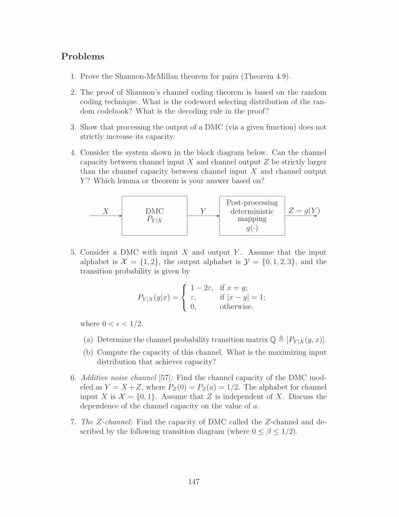
Problems
1. Prove the Shannon-McMillan theorem for pairs (Theorem 4.9).
2. The proof of Shannon’s channel coding theorem is based on the randomcoding technique. What is the codeword selecting distribution of the ran-dom codebook? What is the decoding rule in the proof?
3. Show that processing the output of a DMC (via a given function) does notstrictly increase its capacity.
4. Consider the system shown in the block diagram below. Can the channelcapacity between channel input X and channel output Z be strictly largerthan the channel capacity between channel input X and channel outputY ? Which lemma or theorem is your answer based on?
- DMCPY |X
-
Post-processingdeterministic
mappingg(·)
-X Y Z = g(Y )
5. Consider a DMC with input X and output Y . Assume that the inputalphabet is X = 1, 2, the output alphabet is Y = 0, 1, 2, 3, and thetransition probability is given by
PY |X(y|x) =
1 − 2ε, if x = y;ε, if |x − y| = 1;0, otherwise,
where 0 < ǫ < 1/2.
(a) Determine the channel probability transition matrix Q , [PY |X(y, x)].
(b) Compute the capacity of this channel. What is the maximizing inputdistribution that achieves capacity?
6. Additive noise channel [57]: Find the channel capacity of the DMC mod-eled as Y = X +Z, where PZ(0) = PZ(a) = 1/2. The alphabet for channelinput X is X = 0, 1. Assume that Z is independent of X. Discuss thedependence of the channel capacity on the value of a.
7. The Z-channel: Find the capacity of DMC called the Z-channel and de-scribed by the following transition diagram (where 0 ≤ β ≤ 1/2).
147

-*
-
0
1
0
1
1
β
1 − β
8. Functional representation of the Z-channel: Consider the DMC of Prob-lem 4.7 above.
(a) Give a functional representation of the channel by explicitly express-ing, at any time instant i, the channel output Yi in terms of theinput Xi and a binary noise random variable Zi, which is indepen-dent of the input and is generated from a memoryless process Ziwith Pr[Zi = 0] = β.
(b) Show that the channel’s input-output mutual information satisfies
I(X; Y ) ≥ H(Y ) − H(Z).
(c) Show that the capacity of the Z-channel is no smaller than that of aBSC with crossover probability 1−β (i.e., a binary modulo-2 additivenoise channel with Zi as its noise process):
C ≥ 1 − hb(β)
where hb(·) is the binary entropy function.
9. A DMC has identical input and output alphabets given by 0, 1, 2, 3, 4.Let X be the channel input, and Y be the channel output. Suppose that
PY |X(i|i) =1
2∀ i ∈ 0, 1, 2, 3, 4.
(a) Find the channel transition matrix that maximizes H(Y |X).
(b) Using the channel transition matrix obtained in (a), evaluate thechannel capacity.
10. Binary channel: Consider a binary memoryless channel with the followingprobability transition matrix:
Q =
[1 − α α
β 1 − β
]
,
where α > 0, β > 0 and α + β < 1.
(a) Determine the capacity C of this channel in terms of α and β.
148

(b) What does the expression of C reduces to if α = β ?
11. Find the capacity of the asymmetric binary channel with errors and era-sures described in (4.2.10). Verify that the channel capacity reduces tothat of the BSEC when setting ε′ = ε and α′ = α.
12. Find the capacity of the binary-input quaternary-output DMC given in(4.4.2). For what values of ε is capacity maximized, and for what valuesof ε is capacity minimized ?
13. Non-binary erasure channel: Find the capacity of the q-ary erasure channeldescribed in (4.2.12) and compare the result with the capacity of the BEC.
14. Product of two channels [245]: Consider two DMCs
(X1, PY1|X1 ,Y1) and (X2, PY2|X2 ,Y2)
with capacity C1 and C2 respectively. A new channel (X1 × X2, PY1|X1 ×PY2|X2 ,Y1×Y2) is formed in which x1 ∈ X1 and x2 ∈ X2 are simultaneouslysent, resulting in Y1, Y2. Find the capacity of this channel.
15. The sum channel [245]:
(a) Let (X1, PY1|X1 ,Y1) be a DMC with finite input alphabet X1, finiteoutput alphabet Y1, transition distribution PY1|X1(y|x) and capacityC1. Similarly, let (X2, PY2|X2 ,Y2) be another DMC with capacity C2.Assume that X1 ∩ X2 = ∅ and that Y1 ∩ Y2 = ∅.Now let (X , PY |X ,Y) be the sum of these two channels where X =X1 ∪ X2, Y = Y1 ∪ Y2 and
PY |X(y|x) =
PY1|X1(y|x) if x ∈ X1, y ∈ Y1
PY2|X2(y|x) if x ∈ X2, y ∈ Y2
0 otherwise.
Show that the capacity of the sum channel is given by
Csum = log2
(2C1 + 2C2
)bits/channel use.
Hint: Introduce a Bernoulli random variable Z with Pr[Z = 1] = αsuch that Z = 1 if X ∈ X1 (when the first channel is used), and Z = 2if X ∈ X2 (when the second channel is used). Then show that
I(X; Y ) = I(X,Z; Y )
= hb(α) + αI(X1; Y1) + (1 − α)I(X2; Y2),
where hb(·) is the binary entropy function, and I(Xi; Yi) is the mutualinformation for channel PYi|Xi
(y|x), i = 1, 2. Then maximize (jointly)over the input distribution and α.
149

(b) Compute Csum above if the first channel is a BSC with crossoverprobability 0.11, and the second channel is a BEC with erasure pro-bability 0.5.
16. Prove that the quasi-symmetric channel satisfies the KKT condition ofLemma 4.22 and yields the channel capacity given by (4.4.6).
17. Let the channel transition probability PY |X of a DMC be defined as thefollowing figure, where 0 < ǫ < 0.5.
-
1-
1-
1-
R3
2
1
0
3
2
1
0
1 − ε
1 − ε
1 − ε
ε
ε
ε
1 − ε
ε
(a) Is the channel weakly symmetric? Is the channel symmetric?
(b) Determine the channel capacity of this channel. Also, indicate theinput distribution that achieves the channel capacity.
18. Let the relation between the channel input Xn∞n=1 and channel outputYn∞n=1 be given by
Yn = (αn × Xn) ⊕ Nn for each n,
where αn, Xn, Yn and Nn all take values from 0, 1, and “⊕” representsthe modulo-2 addition operation. Assume that the attenuation αn∞n=1,channel input Xn∞n=1 and noise Nn∞n=1 processes are independent fromeach other. Also, αn∞n=1 and Nn∞n=1 are i.i.d. with
Pr[αn = 1] = Pr[αn = 0] =1
2
andPr[Nn = 1] = 1 − Pr[Nn = 0] = ε ∈ (0, 1/2).
150
(a) Show that the channel is a DMC and derive its transition probabilitymatrix [
PYj |Xj(0|0) PYj |Xj
(1|0)PYj |Xj
(0|1) PYj |Xj(1|1)
]
.
(b) Determine the channel capacity C.
Hint: Use the KKT condition for channel capacity (Lemma 4.22).
(c) Suppose that αn is known, and consists of k 1’s. Find the maximumI(Xn; Y n) for the same channel with known αn.
Hint: For known αn, (Xj, Yj)nj=1 are independent. Recall I(Xn; Y n)
≤ ∑nj=1 I(Xj; Yj).
(d) Some researchers attempt to derive the capacity of the channel in (b)in terms of the following steps:
• Derive the maximum mutual information between channel inputXn and output Y n for a given αn (namely the solution in (c));
• Calculate the expectation value of the maximum mutual informa-tion obtained from the previous step according to the statisticsof αn.
• Then the capacity of the channel is equal to this “expected value”divided by n.
Does this “expected capacity” C coincide with that in (b)?
19. Maximum likelihood vs minimum Hamming distance decoding: Given achannel with finite input and output alphabets X and Y , respectively,and given codebook C = c1, · · · , cM of size M and blocklength n withci = (ci,1, · · · , ci,n) ∈ X n, if an n-tuple yn ∈ Yn is received at the channeloutput, then under maximum likelihood (ML) decoding, yn is decodedinto the codeword c∗ ∈ C that maximizes P (Y n = yn|Xn = c) amongall codewords c ∈ C. It can be shown that ML decoding minimizes theprobability of decoding error when the channel input n-tuple is chosenuniformly among all the codewords.
Recall that the Hamming distance dH(xn, yn) between two n-tuples xn andyn taking values in X n is defined as the number of positions where xn and yn
differ. For a BSC using a binary codebook C = c1, · · · , cM ⊆ 0, 1n ofsize M and blocklength n, if a received n-tuple yn is received at the channeloutput, then under minimum Hamming distance decoding, yn is decodedinto the codeword c ∈ C that minimizes dH(c, yn) among all codewordsc ∈ C.
Prove that minimum Hamming distance decoding is equivalent to ML de-coding for the BSC if its crossover probability ǫ satisfies: ε ≤ 1/2.
151

20. Suppose that blocklength n = 2 and code size M = 2. Assume each codebit is either 0 or 1.
(a) What is the number of all possible codebook designs? (Note: Thisnumber includes those lousy code designs, such as 00, 00.)
(b) Suppose that one randomly draws one of these possible code designsaccording to a uniform distribution and applies the selected code toBSC with crossover probability ε. Then what is the expected errorprobability, if the decoder simply selects the codeword whose Ham-ming distance to the received vector is the smallest? (When bothcodewords have the same Hamming distance to the received vector,the decoder chooses one of them at random as the transmitted code-word.)
(c) Explain why the error in (b) does not vanish as ε ↓ 0.
Hint: The error of random (n,M) code is lower bounded by the errorof random (n, 2) code for M ≥ 2.
21. Fano’s inequality: Assume that the alphabets for random variables X andY are both given by
X = Y = 1, 2, 3, 4, 5.Let
x = g(y)
be an estimate of x from observing y. Define the probability of estimationerror as
Pe = Prg(Y ) 6= X.Then, Fano’s inequality gives a lower bound for Pe as
hb(Pe) + 2Pe ≥ H(X|Y ),
where hb(p) = p log21p
+ (1 − p) log21
1−pis the binary entropy function.
The curve forhb(Pe) + 2Pe = H(X|Y )
in terms of H(X|Y ) versus Pe is plotted in the figure below.
152

0 0.1 0.2 0.3 0.4 0.5 0.6 0.7 0.8 0.9 10
0.5
1
1.5
2
2.5
Pe
H(X
|Y)
(in b
its)
|X|=5
A
B
C
D
(a) Point A on the above figure shows that if H(X|Y ) = 0, zero estimationerror, namely, Pe = 0, can be achieved. In this case, characterize thedistribution PX|Y . Also, give an estimator g(·) that achieves Pe = 0.Hint: Think what kind of relation between X and Y can renderH(X|Y ) = 0.
(b) Point B on the above figure indicates that when H(X|Y ) = log2(5),the estimation error can only be equal to 0.8. In this case, characterizethe distributions PX|Y and PX . Prove that at H(X|Y ) = log2(5), allestimators yield Pe = 0.8.
Hint: Think what kind of relation between X and Y can result inH(X|Y ) = log2(5).
(c) Point C on the above figure hints that when H(X|Y ) = 2, the esti-mation error can be as worse as 1. Give an estimator g(·) that leadsto Pe = 1, if PX|Y (x|y) = 1/4 for x 6= y, and PX|Y (x|y) = 0 for x = y.
(d) Similarly, point D on the above figure hints that when H(X|Y ) = 0,the estimation error can be as worse as 1. Give an estimator g(·) thatleads to Pe = 1 at H(X|Y ) = 0.
22. Decide whether the following statement is true or false. Consider a discretememoryless channel with input alphabet X , output alphabet Y and transi-tion distribution PY |X(y|x) , PrY = y|X = x. Let PX1(·) and PX2(·) betwo possible input distributions, and PY1(·) and PY2(·) be the correspond-ing output distributions; i.e., ∀y ∈ Y , PYi
(y) =∑
x∈X PY |X(y|x)PXi(x),
153
i = 1, 2. ThenD(PX1 ||PX2) ≥ D(PY1 ||PY2).
23. Consider a system consisting of two (parallel) discrete memoryless channelswith transition probability matrices Q1 = [p1(y1|x)] and Q2 = [p2(y2|x)].These channels have a common input alphabet X and output alphabetsY1 and Y2, respectively, where Y1 and Y2 are disjoint. Let X denote thecommon input to the two channels, and let Y1 and Y2 be the correspondingoutputs in channels Q1 and Q2, respectively. Now let Y be an overalloutput of the system which switches between Y1 and Y2 according to thevalues of a binary random variable Z ∈ 1, 2 as follows:
Y =
Y1 if Z = 1;
Y2 if Z = 2;
where Z is independent of the input X and has distribution P (Z = 1) = λ.
(a) Express the system’s mutual information I(X; Y ) in terms of λ, I(X; Y1)and I(X; Y2).
(b) Find an upper bound on the system’s capacity C = maxPXI(X; Y )
in terms of λ, C1 and C2, where Ci is the capacity of channel Qi,i = 1, 2.
(c) If both C1 and C2 can be achieved by the same input distribution,show that the upper bound on C in (b) is exact.
24. Cascade channel: Consider a channel with input alphabet X , output alpha-bet Y and transition probability matrix Q1 = [p1(y|x)]. Consider anotherchannel with input alphabet Y , output alphabet Z and transition proba-bility matrix Q2 = [p2(z|y)]. Let C1 denote the capacity of channel Q1,and let C2 denote the capacity of channel Q2.
Define a new cascade channel with input alphabet X , output alphabet Zand transition probability matrix Q = [p(z|x)] obtained by feeding theoutput of channel Q1 into the input of channel Q2. Let C denote thecapacity of channel Q.
(a) Show that p(z|x) =∑
y∈Y p2(z|y)p1(y|x) and that C ≤ minC1, C2.(b) If X = 0, 1, Y = Z = a, b, c, Q1 is described by
Q1 = [p1(y|x)] =
[1 − α α 0
0 α 1 − α
]
, 0 ≤ α ≤ 1,
154

and Q2 is described by
Q2 = [p2(z|y)] =
1 − ǫ ǫ/2 ǫ/2ǫ/2 1 − ǫ ǫ/2ǫ/2 ǫ/2 1 − ǫ
, 0 ≤ ǫ ≤ 1,
find the capacities C1 and C2.
(c) Given the channels Q1 and Q2 described in part (b), find C in termsof α and ǫ.
(d) Compute the value of C obtained in part (c) if ǫ = 2/3. Explainqualitatively.
25. Let X be a binary random variable with alphabet X = 0, 1. Let Z denoteanother random variable that is independent of X and taking values inZ = 0, 1, 2, 3 such that Pr[Z = 0] = Pr[Z = 1] = Pr[Z = 2] = ǫ, where0 < ǫ ≤ 1/3. Consider a DMC with input X, noise Z, and output Ydescribed by the equation:
Y = 3X + (−1)XZ,
where X and Z are as defined above.
(a) Determine the channel transition probability matrix Q = [p(y|x)].
(b) Compute the capacity C of this channel in terms of ǫ. What is themaximizing input distribution that achieves capacity ?
(c) For what value of ǫ is the noise entropy H(Z) maximized ? What isthe value of C for this choice of ǫ ? Comment on the result.
26. A channel with skewed errors [91]: This problem analyzes a communicationchannel in which the non-zero additive noise generated by the channel canbe partitioned into two distinct sets: the set of “common” errors A andthe set of “uncommon” errors B.
Consider a DMC with identical input and output alphabets given by X =Y = 0, 1, · · · , q − 1 where q is a fixed positive integer. The output Y ofthe channel is related to the input X by the equation
Y = X ⊕ Z,
where Z is a noise random variable with alphabet Z = X = Y , and ⊕denotes addition modulo-q. Assume that Z is independent of X.
We now describe the distribution on Z. Let A and B be the following twosets:
A = 1, 2, · · · , r,
155

andB = r + 1, r + 2, · · · , q − 1,
where integer 0 < r < q − 1 is fixed. Then
• P (Z 6= 0) = ǫ.
• P (Z ∈ A|Z 6= 0) = γ.
• P (Z = i) is constant for all i ∈ A.
• P (Z = j) is constant for all j ∈ B.
(a) Determine P (Z = z) for all z ∈ Z.
(b) Find the capacity of the channel in terms of q, r, ǫ and γ.
(c) What are the values of ǫ and γ that minimize the capacity ? Explainwhy these values make sense intuitively and find the correspondingminimum capacity.
Note: This channel was introduced in [91] to model non-binary data trans-mission and storage channels in which some types of errors (designated as“common errors”) occur much more frequently than others. A family ofcodes, called focused error control codes, was developed in [91] to provide acertain level of protection against the common errors of the channel whileguaranteeing another lower level of protection against uncommon errors;hence the levels of protection are determined based not only on the num-bers of errors but on the kind of errors as well (unlike traditional channelcodes). The performance of these codes was assessed in [6].
27. Memory increases channel capacity: This problem illustrates the adage“memory increases capacity.” Given an integer q ≥ 2, consider a q-aryadditive-noise channel described by
Yi = Xi ⊕ Zi, i = 1, 2 · · · ,
where ⊕ denotes addition modulo-q and Yi, Xi and Zi are the channeloutput, input and noise at time instant i, all with identical alphabetY = X = Z = 0, 1, · · · , q − 1. We assume that the input and noiseprocesses are independent of each other and that the noise process Zi∞i=1
is stationary ergodic. It can be shown via an extended version of Theo-rem 4.10 that the (operational) capacity of this channel with memory isgiven by [67, 140]:
C = limn→∞
maxp(xn)
1
nI(Xn; Y n).
Now consider an “equivalent” memoryless channel in the sense that it hasa memoryless additive noise Zi∞i=1 with identical marginal distribution
156

as noise Zi∞i=1: PZi(z) = PZi
(z) for all i and z ∈ Z. Letting C denotethe capacity of the equivalent memoryless channel, show that
C ≥ C.
Note: The adage “memory increases capacity” does not hold for arbitrarychannels. It is only valid for well-behaved channels with memory [68], suchas the above additive-noise channel with stationary ergodic noise or moregenerally for information stable channels [67, 214, 140] whose capacity isgiven by22
C = lim infn→∞
maxp(xn)
1
nI(Xn; Y n).
However, one can find counter-examples to this adage, such as in [2] regard-ing non-ergodic “averaged” channels [146, 3]. Examples of such averagedchannels include additive-noise channels with stationary but non-ergodicnoise, in particular the Polya-contagion channel [7] whose noise process isdescribed in Example 3.15.
28. Suppose you wish to encode a binary DMS with PX(0) = 3/4 using arate-1 source-channel block code for transmission over a BEC with erasureprobability α. For what values of α, can the source be recovered reliably(i.e., with arbitrarily low error probability) at the receiver ?
29. Consider the binary Polya contagion Markov source of memory two treatedin Problem 3.10; see also Example 3.16 with M = 2. We are interestedin sending this source over the BSC with crossover probability ε usingrate-Rsc block source-channel codes.
(a) Write down the sufficient condition for reliable transmissibility of thesource over the BSC via rate-Rsc source-channel codes in terms of ε,Rsc and the source parameters ρ , R/T and δ , ∆/T .
(b) If ρ = δ = 1/2 and ε = 1/4, determine the of permissible range ofrates Rsc for reliably communicating the source over the channel.
30. Consider a DMC with input alphabet X = 0, 1, 2, 3, 4, output alphabet
22Note that a formula of the capacity of more general (not necessarily information stable)channels with memory does exist in terms of a generalized (spectral) mutual information rate,see [280, 128].
157
Y = 0, 1, 2, 3, 4, 5 and the following transition matrix
Q =
1 − 2α α α 0 0 0α α 1 − 2α 0 0 00 0 0 1 − β β/2 β/20 0 0 β/2 1 − β β/20 0 0 β/2 β/2 1 − β
where 0 < α < 1/2 and 0 < β < 1.
(a) Determine the capacity C of this channel in terms of α and β. Whatis the maximizing input distribution that achieves capacity ?
(b) Find the values of α and β that will yield the smallest possible valueof C.
(c) Show that any (not necessarily memoryless) binary source Ui∞i=1
with arbitrary distribution can be sent without any loss via a rate-one source-channel code over the channel with the parameters α andβ obtained in part (b).
158

Chapter 5
Differential Entropy and GaussianChannels
We have so far examined information measures and their operational character-ization for discrete-time discrete-alphabet systems. In this chapter, we turn ourfocus to continuous-alphabet (real-valued) systems. Except for a brief interludewith the continuous-time (waveform) Gaussian channel, we consider discrete-time systems, as treated throughout the book.
We first recall that a real-valued (continuous) random variable X is describedby its cumulative distribution function (cdf)
FX(x) , Pr[X ≤ x]
for x ∈ R, the set of real numbers. The distribution of X is called absolutely con-tinuous (with respect to the Lebesgue measure) if a probability density function(pdf) fX(·) exists such that
FX(x) =
∫ x
−∞fX(t)dt
where fX(t) ≥ 0 ∀t and∫ +∞−∞ fX(t)dt = 1. If FX(·) is differentiable everywhere,
then the pdf fX(·) exists and is given by the derivative of FX(·): fX(t) = dFX(t)dt
.The support of a random variable X with pdf fX(·) is denoted by SX and canbe conveniently given as
SX = x ∈ R : fX(x) > 0.
We will deal with random variables that admit a pdf.1
1A rigorous (measure-theoretic) study for general continuous systems, initiated by Kol-mogorov [162], can be found in [214, 144].
159
5.1 Differential entropy
Recall that the definition of entropy for a discrete random variable X represent-ing a DMS is
H(X) ,∑
x∈X−PX(x) log2 PX(x) (in bits).
As already seen in Shannon’s source coding theorem, this quantity is the mini-mum average code rate achievable for the lossless compression of the DMS. But ifthe random variable takes on values in a continuum, the minimum number of bitsper symbol needed to losslessly describe it must be infinite. This is illustratedin the following example, where we take a discrete approximation (quantization)of a random variable uniformly distributed on the unit interval and study theentropy of the quantized random variable as the quantization becomes finer andfiner.
Example 5.1 Consider a real-valued random variable X that is uniformly dis-tributed on the unit interval, i.e., with pdf given by
fX(x) =
1 if x ∈ [0, 1);
0 otherwise.
Given a positive integer m, we can discretize X by uniformly quantizing it intom levels by partitioning the support of X into equal-length segments of size∆ = 1
m(∆ is called the quantization step-size) such that:
qm(X) =i
m, if
i − 1
m≤ X <
i
m,
for 1 ≤ i ≤ m. Then the entropy of the quantized random variable qm(X) isgiven by
H(qm(X)) = −m∑
i=1
1
mlog2
(1
m
)
= log2 m (in bits).
Since the entropy H(qm(X)) of the quantized version of X is a lower bound tothe entropy of X (as qm(X) is a function of X) and satisfies in the limit
limm→∞
H(qm(X)) = limm→∞
log2 m = ∞,
we obtain that the entropy of X is infinite.
The above example indicates that to compress a continuous source withoutincurring any loss or distortion indeed requires an infinite number of bits. Thus
160

when studying continuous sources, the entropy measure is limited in its effective-ness and the introduction of a new measure is necessary. Such new measure isindeed obtained upon close examination of the entropy of a uniformly quantizedreal-valued random-variable minus the quantization accuracy as the accuracyincreases without bound.
Lemma 5.2 Consider a real-valued random variable X with support [a, b) and
pdf fX such that −fX log2 fX is integrable2 (where −∫ b
afX(x) log2 fX(x)dx is
finite). Then a uniform quantization of X with an n-bit accuracy (i.e., witha quantization step-size of ∆ = 2−n) yields an entropy approximately equal to
−∫ b
afX(x) log2 fX(x)dx + n bits for n sufficiently large. In other words,
limn→∞
[H(qn(X)) − n] = −∫ b
a
fX(x) log2 fX(x)dx
where qn(X) is the uniformly quantized version of X with quantization step-size∆ = 2−n.
Proof:
Step 1: Mean-value theorem. Let ∆ = 2−n be the quantization step-size,and let
ti ,
a + i∆, i = 0, 1, · · · , j − 1
b, i = j
where j = ⌈(b − a)2n⌉. From the mean-value theorem (e.g., cf. [186]), wecan choose xi ∈ [ti−1, ti] for 1 ≤ i ≤ j such that
pi ,
∫ ti
ti−1
fX(x)dx = fX(xi)(ti − ti−1) = ∆ · fX(xi).
Step 2: Definition of h(n)(X). Let
h(n)(X) , −j∑
i=1
[fX(xi) log2 fX(xi)]2−n.
Since −fX(x) log2 fX(x) is integrable,
h(n)(X) → −∫ b
a
fX(x) log2 fX(x)dx as n → ∞.
Therefore, given any ε > 0, there exists N such that for all n > N ,∣∣∣∣−∫ b
a
fX(x) log2 fX(x)dx − h(n)(X)
∣∣∣∣< ε.
2By integrability, we mean the usual Riemann integrability (e.g, see [233]).
161

Step 3: Computation of H(qn(X)). The entropy of the (uniformly) quan-tized version of X, qn(X), is given by
H(qn(X)) = −j∑
i=1
pi log2 pi
= −j∑
i=1
(fX(xi)∆) log2(fX(xi)∆)
= −j∑
i=1
(fX(xi)2−n) log2(fX(xi)2
−n)
where the pi’s are the probabilities of the different values of qn(X).
Step 4: H(qn(X)) − h(n)(X) .
From Steps 2 and 3,
H(qn(X)) − h(n)(X) = −j∑
i=1
[fX(xi)2−n] log2(2
−n)
= n
j∑
i=1
∫ ti
ti−1
fX(x)dx
= n
∫ b
a
fX(x)dx = n.
Hence, we have that for n > N ,
[
−∫ b
a
fX(x) log2 fX(x)dx + n
]
− ε < H(qn(X))
= h(n)(X) + n
<
[
−∫ b
a
fX(x) log2 fX(x)dx + n
]
+ ε,
yielding that
limn→∞
[H(qn(X)) − n] = −∫ b
a
fX(x) log2 fX(x)dx.
2
More generally, the following result due to Renyi [227] can be shown for (abso-lutely continuous) random variables with arbitrary support.
162

Theorem 5.3 [227, Theorem 1] For any real-valued random variable with pdffX , if −∑i pi log2 pi is finite, where the (possibly countably many) pi’s are theprobabilities of the different values of the uniformly quantized qn(X) over supportSX , then
limn→∞
[H(qn(X)) − n] = −∫
SX
fX(x) log2 fX(x)dx
provided the integral on the right-hand side exists.
In light of the above results, we can define the following information measure.
Definition 5.4 (Differential entropy) The differential entropy (in bits) of acontinuous random variable X with pdf fX and support SX is defined as
h(X) , −∫
SX
fX(x) · log2 fX(x)dx = E[− log2 fX(X)],
when the integral exists.
Thus the differential entropy h(X) of a real-valued random variable X hasan operational meaning in the following sense. Since H(qn(X)) is the minimumaverage number of bits needed to losslessly describe qn(X), we thus obtain thath(X) + n is approximately needed to describe X when uniformly quantizing itwith an n-bit accuracy. Therefore, we may conclude that the larger h(X) is, thelarger is the average number of bits required to describe a uniformly quantizedX within a fixed accuracy.
Example 5.5 A continuous random variable X with support SX = [0, 1) andpdf fX(x) = 2x for x ∈ SX has differential entropy equal to
∫ 1
0
−2x · log2(2x)dx =x2(log2 e − 2 log2(2x))
2
∣∣∣∣
1
0
=1
2 ln 2− log2(2) = −0.278652 bits.
We herein illustrate Lemma 5.2 by uniformly quantizing X to an n-bit accuracyand computing the entropy H(qn(X)) and H(qn(X))−n for increasing values ofn, where qn(X) is the quantized version of X.
We have that qn(X) is given by
qn(X) =i
2n, if
i − 1
2n≤ X <
i
2n,
163
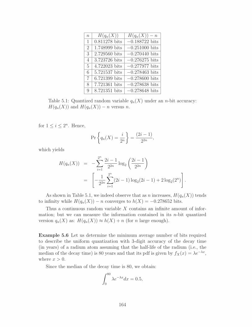
n H(qn(X)) H(qn(X)) − n1 0.811278 bits −0.188722 bits2 1.748999 bits −0.251000 bits3 2.729560 bits −0.270440 bits4 3.723726 bits −0.276275 bits5 4.722023 bits −0.277977 bits6 5.721537 bits −0.278463 bits7 6.721399 bits −0.278600 bits8 7.721361 bits −0.278638 bits9 8.721351 bits −0.278648 bits
Table 5.1: Quantized random variable qn(X) under an n-bit accuracy:H(qn(X)) and H(qn(X)) − n versus n.
for 1 ≤ i ≤ 2n. Hence,
Pr
qn(X) =i
2n
=(2i − 1)
22n,
which yields
H(qn(X)) = −2n∑
i=1
2i − 1
22nlog2
(2i − 1
22n
)
=
[
− 1
22n
2n∑
i=1
(2i − 1) log2(2i − 1) + 2 log2(2n)
]
.
As shown in Table 5.1, we indeed observe that as n increases, H(qn(X)) tendsto infinity while H(qn(X)) − n converges to h(X) = −0.278652 bits.
Thus a continuous random variable X contains an infinite amount of infor-mation; but we can measure the information contained in its n-bit quantizedversion qn(X) as: H(qn(X)) ≈ h(X) + n (for n large enough).
Example 5.6 Let us determine the minimum average number of bits requiredto describe the uniform quantization with 3-digit accuracy of the decay time(in years) of a radium atom assuming that the half-life of the radium (i.e., themedian of the decay time) is 80 years and that its pdf is given by fX(x) = λe−λx,where x > 0.
Since the median of the decay time is 80, we obtain:∫ 80
0
λe−λxdx = 0.5,
164

which implies that λ = 0.00866. Also, 3-digit accuracy is approximately equiv-alent to log2 999 = 9.96 ≈ 10 bits accuracy. Therefore, by Theorem 5.3, thenumber of bits required to describe the quantized decay time is approximately
h(X) + 10 = log2
e
λ+ 10 = 18.29 bits.
We close this section by computing the differential entropy for two commonreal-valued random variables: the uniformly distributed random variable andthe Gaussian distributed random variable.
Example 5.7 (Differential entropy of a uniformly distributed randomvariable) Let X be a continuous random variable that is uniformly distributedover the interval (a, b), where b > a; i.e., its pdf is given by
fX(x) =
1
b−aif x ∈ (a, b);
0 otherwise.
So its differential entropy is given by
h(X) = −∫ b
a
1
b − alog2
1
b − a= log2(b − a) bits.
Note that if (b − a) < 1 in the above example, then h(X) is negative, unlikeentropy. The above example indicates that although differential entropy has aform analogous to entropy (in the sense that summation and pmf for entropy arereplaced by integration and pdf, respectively, for differential entropy), differen-tial entropy does not retain all the properties of entropy (one such operationaldifference was already highlighted in the previous lemma and theorem).3
Example 5.8 (Differential entropy of a Gaussian random variable) LetX ∼ N (µ, σ2); i.e., X is a Gaussian (or normal) random variable with finite meanµ, variance Var(X) = σ2 > 0 and pdf
fX(x) =1√
2πσ2e−
(x−µ)2
2σ2
for x ∈ R. Then its differential entropy is given by
h(X) =
∫
R
fX(x)
[1
2log2(2πσ2) +
(x − µ)2
2σ2log2 e
]
dx
3By contrast, entropy and differential entropy are sometimes called discrete entropy andcontinuous entropy, respectively.
165
=1
2log2(2πσ2) +
log2 e
2σ2E[(X − µ)2]
=1
2log2(2πσ2) +
1
2log2 e
=1
2log2(2πeσ2) bits. (5.1.1)
Note that for a Gaussian random variable, its differential entropy is only a func-tion of its variance σ2 (it is independent from its mean µ). This is similar tothe differential entropy of a uniform random variable, which only depends ondifference (b − a) but not the mean (a + b)/2.
5.2 Joint and conditional differential entropies, divergenceand mutual information
Definition 5.9 (Joint differential entropy) If Xn = (X1, X2, · · · , Xn) is acontinuous random vector of size n (i.e., a vector of n continuous random vari-ables) with joint pdf fXn and support SXn ⊆ Rn, then its joint differentialentropy is defined as
h(Xn) , −∫
SXn
fXn(x1, x2, · · · , xn) log2 fXn(x1, x2, · · · , xn) dx1 dx2 · · · dxn
= E[− log2 fXn(Xn)]
when the n-dimensional integral exists.
Definition 5.10 (Conditional differential entropy) Let X and Y be twojointly distributed continuous random variables with joint pdf4 fX,Y and supportSX,Y ⊆ R2 such that the conditional pdf of Y given X, given by
fY |X(y|x) =fX,Y (x, y)
fX(x),
is well defined for all (x, y) ∈ SX,Y , where fX is the marginal pdf of X. Thenthe conditional entropy of Y given X is defined as
h(Y |X) , −∫
SX,Y
fX,Y (x, y) log2 fY |X(y|x) dx dy = E[− log2 fY |X(Y |X)],
when the integral exists.
4Note that the joint pdf fX,Y is also commonly written as fXY .
166

Note that as in the case of (discrete) entropy, the chain rule holds for differ-ential entropy:
h(X,Y ) = h(X) + h(Y |X) = h(Y ) + h(X|Y ).
Definition 5.11 (Divergence or relative entropy) Let X and Y be two con-tinuous random variables with marginal pdfs fX and fY , respectively, such thattheir supports satisfy SX ⊆ SY ⊆ R. Then the divergence (or relative entropy orKullback-Leibler distance) between X and Y is written as D(X‖Y ) or D(fX‖fY )and defined by
D(X‖Y ) ,
∫
SX
fX(x) log2
fX(x)
fY (x)dx = E
[fX(X)
fY (X)
]
when the integral exists. The definition carries over similarly in the multivariatecase: for Xn = (X1, X2, · · · , Xn) and Y n = (Y1, Y2, · · · , Yn) two random vectorswith joint pdfs fXn and fY n , respectively, and supports satisfying SXn ⊆ SY n ⊆Rn, the divergence between Xn and Y n is defined as
D(Xn‖Y n) ,
∫
SXn
fXn(x1, x2, · · · , xn) log2
fXn(x1, x2, · · · , xn)
fY n(x1, x2, · · · , xn)dx1 dx2 · · · dxn
when the integral exists.
Definition 5.12 (Mutual information) Let X and Y be two jointly distributedcontinuous random variables with joint pdf fX,Y and support SXY ⊆ R2. Thenthe mutual information between X and Y is defined by
I(X; Y ) , D(fX,Y ‖fXfY ) =
∫
SX,Y
fX,Y (x, y) log2
fX,Y (x, y)
fX(x)fY (y)dx dy,
assuming the integral exists, where fX and fY are the marginal pdfs of X andY , respectively.
Observation 5.13 For two jointly distributed continuous random variables Xand Y with joint pdf fX,Y , support SXY ⊆ R2 and joint differential entropy
h(X,Y ) = −∫
SXY
fX,Y (x, y) log2 fX,Y (x, y) dx dy,
then as in Lemma 5.2 and the ensuing discussion, one can write
H(qn(X), qm(Y )) ≈ h(X,Y ) + n + m
167
for n and m sufficiently large, where qk(Z) denotes the (uniformly) quantizedversion of random variable Z with a k-bit accuracy.
On the other hand, for the above continuous X and Y ,
I(qn(X); qm(Y )) = H(qn(X)) + H(qm(Y )) − H(qn(X), qm(Y ))
≈ [h(X) + n] + [h(Y ) + m] − [h(X,Y ) + n + m]
= h(X) + h(Y ) − h(X,Y )
=
∫
SX,Y
fX,Y (x, y) log2
fX,Y (x, y)
fX(x)fY (y)dx dy
for n and m sufficiently large; in other words,
limn,m→∞
I(qn(X); qm(Y )) = h(X) + h(Y ) − h(X,Y ).
Furthermore, it can be shown that
limn→∞
D(qn(X)‖qn(Y )) =
∫
SX
fX(x) log2
fX(x)
fY (x)dx.
Thus mutual information and divergence can be considered as the true toolsof Information Theory, as they retain the same operational characteristics andproperties for both discrete and continuous probability spaces (as well as generalspaces where they can be defined in terms of Radon-Nikodym derivatives (e.g.,cf. [144]).5
The following lemma illustrates that for continuous systems, I(·; ·) and D(·‖·)keep the same properties already encountered for discrete systems, while differ-ential entropy (as already seen with its possibility if being negative) satisfiessome different properties from entropy. The proof is left as an exercise.
Lemma 5.14 The following properties hold for the information measures ofcontinuous systems.
1. Non-negativity of divergence: Let X and Y be two continuous ran-dom variables with marginal pdfs fX and fY , respectively, such that theirsupports satisfy SX ⊆ SY ⊆ R. Then
D(fX‖fY ) ≥ 0
with equality iff fX(x) = fY (x) for all x ∈ SX except in a set of fX-measurezero (i.e., X = Y almost surely).
5This justifies using identical notations for both I(·; ·) and D(·‖·) as opposed to the dis-cerning notations of H(·) for entropy and h(·) for differential entropy.
168

2. Non-negativity of mutual information: For any two continuous jointlydistributed random variables X and Y ,
I(X; Y ) ≥ 0
with equality iff X and Y are independent.
3. Conditioning never increases differential entropy: For any two con-tinuous random variables X and Y with joint pdf fX,Y and well-definedconditional pdf fX|Y ,
h(X|Y ) ≤ h(X)
with equality iff X and Y are independent.
4. Chain rule for differential entropy: For a continuous random vectorXn = (X1, X2, · · · , Xn),
h(X1, X2, . . . , Xn) =n∑
i=1
h(Xi|X1, X2, . . . , Xi−1),
where h(Xi|X1, X2, . . . , Xi−1) , h(X1) for i = 1.
5. Chain rule for mutual information: For continuous random vectorXn = (X1, X2, · · · , Xn) and random variable Y with joint pdf fXn,Y andwell-defined conditional pdfs fXi,Y |Xi−1 , fXi|Xi−1 and fY |Xi−1 for i = 1, · · · , n,we have that
I(X1, X2, · · · , Xn; Y ) =n∑
i=1
I(Xi; Y |Xi−1, · · · , X1),
where I(Xi; Y |Xi−1, · · · , X1) , I(X1; Y ) for i = 1.
6. Data processing inequality: For continuous random variables X, Yand Z such that X → Y → Z, i.e., X and Z are conditional independentgiven Y ,
I(X; Y ) ≥ I(X; Z).
7. Independence bound for differential entropy: For a continuous ran-dom vector Xn = (X1, X2, · · · , Xn),
h(Xn) ≤n∑
i=1
h(Xi)
with equality iff all the Xi’s are independent from each other.
169

8. Invariance of differential entropy under translation: For continuousrandom variables X and Y with joint pdf fX,Y and well-defined conditionalpdf fX|Y ,
h(X + c) = h(X) for any constant c ∈ R,
andh(X + Y |Y ) = h(X|Y ).
The results also generalize in the multivariate case: for two continuousrandom vectors Xn = (X1, X2, · · · , Xn) and Y n = (Y1, Y2, · · · , Yn) withjoint pdf fXn,Y n and well-defined conditional pdf fXn|Y n ,
h(Xn + cn) = h(Xn)
for any constant n-tuple cn = (c1, c2, · · · , cn) ∈ Rn, and
h(Xn + Y n|Y n) = h(Xn|Y n),
where the addition of two n-tuples is performed component-wise.
9. Differential entropy under scaling: For any continuous random vari-able X and any non-zero real constant a,
h(aX) = h(X) + log2 |a|.
10. Joint differential entropy under linear mapping: Consider the ran-dom (column) vector X = (X1, X2, · · · , Xn)T with joint pdf fXn , where Tdenotes transposition, and let Y = (Y1, Y2, · · · , Yn)T be a random (column)vector obtained from the linear transformation Y = AX, where A is aninvertible (non-singular) n × n real-valued matrix. Then
h(Y ) = h(Y1, Y2, · · · , Yn) = h(X1, X2, · · · , Xn) + log2 |det(A)|,
where det(A) is the determinant of the square matrix A.
11. Joint differential entropy under nonlinear mapping: Consider therandom (column) vector X = (X1, X2, · · · , Xn)T with joint pdf fXn , andlet Y = (Y1, Y2, · · · , Yn)T be a random (column) vector obtained from thenonlinear transformation
Y = g(X) , (g1(X1), g2(X2), · · · , gn(Xn))T ,
where each gi : R → R is a differentiable function, i = 1, 2, · · · , n. Then
h(Y ) = h(Y1, Y2, · · · , Yn)
170

= h(X1, · · · , Xn) +
∫
Rn
fXn(x1, · · · , xn) log2 |det(J)| dx1 · · · dxn,
where J is the n × n Jacobian matrix given by
J ,
∂g1
∂x1
∂g1
∂x2· · · ∂g1
∂xn∂g2
∂x1
∂g2
∂x2· · · ∂g2
∂xn...
... · · · ...∂gn
∂x1
∂gn
∂x2· · · ∂gn
∂xn
.
Observation 5.15 Property 9 of the above Lemma indicates that for a contin-uous random variable X, h(X) 6= h(aX) (except for the trivial case of a = 1)and hence differential entropy is not in general invariant under invertible maps.This is in contrast to entropy, which is always invariant under invertible maps:given a discrete random variable X with alphabet X ,
H(f(X)) = H(X)
for all invertible maps f : X → Y , where Y is a discrete set; in particularH(aX) = H(X) for all non-zero reals a.
On the other hand, for both discrete and continuous systems, mutual infor-mation and divergence are invariant under invertible maps:
I(X; Y ) = I(g(X); Y ) = I(g(X); h(Y ))
andD(X‖Y ) = D(g(X)‖g(Y ))
for all invertible maps g and h properly defined on the alphabet/support of theconcerned random variables. This reinforces the notion that mutual informationand divergence constitute the true tools of Information Theory.
Definition 5.16 (Multivariate Gaussian) A continuous random vector X =(X1, X2, · · · , Xn)T is called a size-n (multivariate) Gaussian random vector witha finite mean vector µ , (µ1, µ2, · · · , µn)T , where µi , E[Xi] < ∞ for i =1, 2, · · · , n, and an n × n invertible (real-valued) covariance matrix
KX = [Ki,j]
, E[(X − µ)(X − µ)T ]
=
Cov(X1, X1) Cov(X1, X2) · · · Cov(X1, Xn)Cov(X2, X1) Cov(X2, X2) · · · Cov(X2, Xn)
...... · · · ...
Cov(Xn, X1) Cov(Xn, X2) · · · Cov(Xn, Xn)
,
171

where Ki,j = Cov(Xi, Xj) , E[(Xi−µi)(Xj −µj)] is the covariance6 between Xi
and Xj for i, j = 1, 2, · · · , n, if its joint pdf is given by the multivariate Gaussianpdf
fXn(x1, x2, · · · , xn) =1
(√
2π)n√
det(KX)e−
12(x−µ)T K−1
X (x−µ)
for any (x1, x2, · · · , xn) ∈ Rn, where x = (x1, x2, · · · , xn)T . As in the scalar case(i.e., for n = 1), we write X ∼ Nn(µ,KX) to denote that X is a size-n Gaussianrandom vector with mean vector µ and covariance matrix KX .
Observation 5.17 In light of the above definition, we make the following re-marks.
1. Note that a covariance matrix K is always symmetric (i.e., KT = K)and positive-semidefinite.7 But as we require KX to be invertible in thedefinition of the multivariate Gaussian distribution above, we will hereafterassume that the covariance matrix of Gaussian random vectors is positive-definite (which is equivalent to having all the eigenvalues of KX positive),thus rendering the matrix invertible.
2. If a random vector X = (X1, X2, · · · , Xn)T has a diagonal covariance ma-trix KX (i.e., all the off-diagonal components of KX are zero: Ki,j = 0for all i 6= j, i, j = 1, · · · , n), then all its component random variables areuncorrelated but not necessarily independent. However, if X is Gaussianand have a diagonal covariance matrix, then all its component randomvariables are independent from each other.
3. Any linear transformation of a Gaussian random vector yields anotherGaussian random vector. Specifically, if X ∼ Nn(µ,KX) is a size-n Gaus-sian random vector with mean vector µ and covariance matrix KX , and ifY = AmnX, where Amn is a given m × n real-valued matrix, then
Y ∼ Nm(Amnµ,AmnKXATmn)
6Note that the diagonal components of KX yield the variance of the different randomvariables: Ki,i = Cov(Xi,Xi) = Var(Xi) = σ2
Xi, i = 1, · · · , n.
7An n×n real-valued symmetric matrix K is positive-semidefinite (e.g., cf. [90]) if for everyreal-valued vector x = (x1, x2 · · · , xn)T ,
xTKx = (x1, · · · , xn)K
x1
...xn
≥ 0,
with equality holding only when xi = 0 for i = 1, 2, · · · , n. Furthermore, the matrix is positive-definite if xT
Kx > 0 for all real-valued vectors x 6= 0, where 0 is the all-zero vector of sizen.
172
is a size-m Gaussian random vector with mean vector Amnµ and covariance
matrix AmnKXATmn.
More generally, any affine transformation of a Gaussian random vectoryields another Gaussian random vector: if X ∼ Nn(µ,KX) and Y =AmnX + bm, where Amn is a m × n real-valued matrix and bm is a size-mreal-valued vector, then
Y ∼ Nm(Amnµ + bm,AmnKXATmn).
Theorem 5.18 (Joint differential entropy of the multivariate Gaussian)If X ∼ Nn(µ,KX) is a Gaussian random vector with mean vector µ and (positive-definite) covariance matrix KX , then its joint differential entropy is given by
h(X) = h(X1, X2, · · · , Xn) =1
2log2 [(2πe)ndet(KX)] . (5.2.1)
In particular, in the univariate case of n = 1, (5.2.1) reduces to (5.1.1).
Proof: Without loss of generality we assume that X has a zero mean vectorsince its differential entropy is invariant under translation by Property 8 ofLemma 5.14:
h(X) = h(X − µ);
so we assume that µ = 0.
Since the covariance matrix KX is a real-valued symmetric matrix, thenit is orthogonally diagonizable; i.e., there exits a square (n × n) orthogonalmatrix A (i.e., satisfying AT = A−1) such that AKXAT is a diagonal ma-trix whose entries are given by the eigenvalues of KX (A is constructed usingthe eigenvectors of KX ; e.g., see [90]). As a result the linear transformationY = AX ∼ Nn
(0,AKXAT
)is a Gaussian vector with the diagonal covariance
matrix KY = AKXAT and has therefore independent components (as noted inObservation 5.17). Thus
h(Y ) = h(Y1, Y2, · · · , Yn)
= h(Y1) + h(Y2) + · · · + h(Yn) (5.2.2)
=n∑
i=1
1
2log2 [2πeVar(Yi)] (5.2.3)
=n
2log2(2πe) +
1
2log2
[n∏
i=1
Var(Yi)
]
=n
2log2(2πe) +
1
2log2 [det (KY )] (5.2.4)
173

=1
2log2 (2πe)n +
1
2log2 [det (KX)] (5.2.5)
=1
2log2 [(2πe)n det (KX)] , (5.2.6)
where (5.2.2) follows by the independence of the random variables Y1, . . . , Yn
(e.g., see Property 7 of Lemma 5.14), (5.2.3) follows from (5.1.1), (5.2.4) holdssince the matrix KY is diagonal and hence its determinant is given by the productof its diagonal entries, and (5.2.5) holds since
det (KY ) = det(AKXAT
)
= det(A)det (KX) det(AT )
= det(A)2det (KX)
= det (KX) ,
where the last equality holds since (det(A))2 = 1, as the matrix A is orthogonal(AT = A−1 =⇒ det(A) = det(AT ) = 1/[det(A)]; thus, det(A)2 = 1).
Now invoking Property 10 of Lemma 5.14 and noting that |det(A)| = 1 yieldthat
h(Y1, Y2, · · · , Yn) = h(X1, X2, · · · , Xn) + log2 |det(A)|︸ ︷︷ ︸
=0
= h(X1, X2, · · · , Xn).
We therefore obtain using (5.2.6) that
h(X1, X2, · · · , Xn) =1
2log2 [(2πe)n det (KX)] ,
hence completing the proof.
An alternate (but rather mechanical) proof to the one presented above con-sists of directly evaluating the joint differential entropy of X by integrating−fXn(xn) log2 fXn(xn) over Rn; it is left as an exercise. 2
Corollary 5.19 (Hadamard’s inequality) For any real-valued n×n positive-definite matrix K = [Ki,j]i,j=1,··· ,n,
det(K) ≤n∏
i=1
Ki,i
with equality iff K is a diagonal matrix, where Ki,i are the diagonal entries ofK.
174

Proof: Since every positive-definite matrix is a covariance matrix (e.g., see[120]), let X = (X1, X2, · · · , Xn)T ∼ Nn (0,K) be a jointly Gaussian randomvector with zero mean vector and covariance matrix K. Then
1
2log2 [(2πe)n det(K)] = h(X1, X2, · · · , Xn) (5.2.7)
≤n∑
i=1
h(Xi) (5.2.8)
=n∑
i=1
1
2log2 [2πeVar(Xi)] (5.2.9)
=1
2log2
[
(2πe)nn∏
i=1
Ki,i
]
, (5.2.10)
where (5.2.7) follows from Theorem 5.18, (5.2.8) follows from Property 7 ofLemma 5.14 and (5.2.9)-(5.2.10) hold using (5.1.1) along with the fact thateach random variable Xi ∼ N (0, Ki,i) is Gaussian with zero mean and varianceVar(Xi) = Ki,i for i = 1, 2, · · · , n (as the marginals of a multivariate Gaussianare also Gaussian (e,g., cf. [120])).
Finally, from (5.2.10), we directly obtain that
det(K) ≤n∏
i=1
Ki,i,
with equality iff the jointly Gaussian random variables X1, X2, . . ., Xn are inde-pendent from each other, or equivalently iff the covariance matrix K is diagonal.
2
The next theorem states that among all real-valued size-n random vectors (ofsupport Rn) with identical mean vector and covariance matrix, the Gaussianrandom vector has the largest differential entropy.
Theorem 5.20 (Maximal differential entropy for real-valued randomvectors) Let X = (X1, X2, · · · , Xn)T be a real-valued random vector with ajoint pdf of support SXn = Rn, mean vector µ, covariance matrix KX and finitejoint differential entropy h(X1, X2, · · · , Xn). Then
h(X1, X2, · · · , Xn) ≤ 1
2log2 [(2πe)n det(KX)] , (5.2.11)
with equality iff X is Gaussian; i.e., X ∼ Nn
(µ,KX
).
175

Proof: We will present the proof in two parts: the scalar or univariate case, andthe multivariate case.
(i) Scalar case (n = 1): For a real-valued random variable with support SX = R,mean µ and variance σ2, let us show that
h(X) ≤ 1
2log2
(2πeσ2
), (5.2.12)
with equality iff X ∼ N (µ, σ2).
For a Gaussian random variable Y ∼ N (µ, σ2), using the non-negativity ofdivergence, can write
0 ≤ D(X‖Y )
=
∫
R
fX(x) log2
fX(x)
1√2πσ2
e−(x−µ)2
2σ2
dx
= −h(X) +
∫
R
fX(x)
[
log2
(√2πσ2
)
+(x − µ)2
2σ2log2 e
]
dx
= −h(X) +1
2log2(2πσ2) +
log2 e
2σ2
∫
R
(x − µ)2fX(x) dx
︸ ︷︷ ︸
=σ2
= −h(X) +1
2log2
[2πeσ2
].
Thus
h(X) ≤ 1
2log2
[2πeσ2
],
with equality iff X = Y (almost surely); i.e., X ∼ N (µ, σ2).
(ii). Multivariate case (n > 1): As in the proof of Theorem 5.18, we can use anorthogonal square matrix A (i.e., satisfying AT = A−1 and hence |det(A)| = 1)such that AKXAT is diagonal. Therefore, the random vector generated by thelinear map
Z = AX
will have a covariance matrix given by KZ = AKXAT and hence have uncorre-lated (but not necessarily independent) components. Thus
h(X) = h(Z) − log2 |det(A)|︸ ︷︷ ︸
=0
(5.2.13)
= h(Z1, Z2, · · · , Zn)
≤n∑
i=1
h(Zi) (5.2.14)
176

≤n∑
i=1
1
2log2 [2πeVar(Zi)] (5.2.15)
=n
2log2(2πe) +
1
2log2
[n∏
i=1
Var(Zi)
]
=1
2log2 (2πe)n +
1
2log2 [det (KZ)] (5.2.16)
=1
2log2 (2πe)n +
1
2log2 [det (KX)] (5.2.17)
=1
2log2 [(2πe)n det (KX)] ,
where (5.2.13) holds by Property 10 of Lemma 5.14 and since |det(A)| = 1,(5.2.14) follows from Property 7 of Lemma 5.14, (5.2.15) follows from (5.2.12)(the scalar case above), (5.2.16) holds since KZ is diagonal, and (5.2.17) followsfrom the fact that det (KZ) = det (KX) (as A is orthogonal). Finally, equality isachieved in both (5.2.14) and (5.2.15) iff the random variables Z1, Z2, . . ., Zn areGaussian and independent from each other, or equivalently iff X ∼ Nn
(µ,KX
).
2
Observation 5.21 (Examples of maximal differential entropy under var-ious constraints) The following three results can also be shown (the proof isleft as an exercise):
1. Among all continuous random variables admitting a pdf with support theinterval (a, b), where b > a are real numbers, the uniformly distributedrandom variable maximizes differential entropy.
2. Among all continuous random variables admitting a pdf with support theinterval [0,∞), finite mean µ and finite differential entropy, the expo-nentially distributed random variable with parameter (or rate parameter)λ = 1/µ maximizes differential entropy.
3. Among all continuous random variables admitting a pdf with support R,finite mean µ and finite differential entropy and satisfying E[|X −µ|] = λ,where λ > 0 is a fixed finite parameter, the Laplacian random variablewith mean µ, variance 2λ2 and pdf
fX(x) =1
2λe−
|x−µ|λ for x ∈ R
maximizes differential entropy.
A systematic approach to finding distributions that maximize differential entropysubject to various support and moments constraints can be found in [57, 294].
177

Observation 5.22 (Information rates for stationary Gaussian sources)We close this section by noting that for stationary Gaussian processes Xiand Xi, the differential entropy rate, limn→∞
1nh(Xn), the divergence rate,
limn→∞1nD(PXn‖PXn), as well as their Renyi counterparts all exist and admit
analytical expressions in terms of the sources power spectral densities [163, 144,277, 113], [106, Table 4].
5.3 AEP for continuous memoryless sources
The AEP theorem and its consequence for discrete memoryless (i.i.d.) sourcesreveal to us that the number of elements in the typical set is approximately2nH(X), where H(X) is the source entropy, and that the typical set carries al-most all the probability mass asymptotically (see Theorems 3.3 and 3.4). Anextension of this result from discrete to continuous memoryless sources by justcounting the number of elements in a continuous (typical) set defined via a lawof large numbers argument is not possible, since the total number of elementsin a continuous set is infinite. However, when considering the volume of thatcontinuous typical set (which is a natural analog to the size of a discrete set),such an extension, with differential entropy playing a similar role as entropy,becomes straightforward.
Theorem 5.23 (AEP for continuous memoryless sources) Let Xi∞i=1 bea continuous memoryless source (i.e., an infinite sequence of continuous i.i.d. ran-dom variables) with pdf fX(·) and differential entropy h(X). Then
− 1
nlog fX(X1, . . . , Xn) → E[− log2 fX(X)] = h(X) in probability.
Proof: The proof is an immediate result of the law of large numbers (e.g., seeTheorem 3.3). 2
Definition 5.24 (Typical set) For δ > 0 and any n given, define the typicalset for the above continuous source as
Fn(δ) ,
xn ∈ Rn :
∣∣∣∣− 1
nlog2 fX(X1, . . . , Xn) − h(X)
∣∣∣∣< δ
.
Definition 5.25 (Volume) The volume of a set A ⊂ Rn is defined as
Vol(A) ,
∫
Adx1 · · · dxn.
178

Theorem 5.26 (Consequence of the AEP for continuous memorylesssources) For a continuous memoryless source Xi∞i=1 with differential entropyh(X), the following hold.
1. For n sufficiently large, PXn Fn(δ) > 1 − δ.
2. Vol(Fn(δ))≤ 2n(h(X)+δ) for all n.
3. Vol(Fn(δ))≥ (1 − δ)2n(h(X)−δ) for n sufficiently large.
Proof: The proof is quite analogous to the corresponding theorem for discretememoryless sources (Theorem 3.4) and is left as an exercise. 2
5.4 Capacity and channel coding theorem for the discrete-time memoryless Gaussian channel
We next study the fundamental limits for error-free communication over thediscrete-time memoryless Gaussian channel, which is the most important cont-inuous-alphabet channel and is widely used to model real-world wired and wire-less channels. We first state the definition of discrete-time continuous-alphabetmemoryless channels.
Definition 5.27 (Discrete-time continuous memoryless channels) Con-sider a discrete-time channel with continuous input and output alphabets givenby X ⊆ R and Y ⊆ R, respectively, and described by a sequence of n-dimensionaltransition (conditional) pdfs fY n|Xn(yn|xn)∞n=1 that govern the reception ofyn = (y1, y2, · · · , yn) ∈ Yn at the channel output when xn = (x1, x2, · · · , xn) ∈X n is sent as the channel input.
The channel (without feedback) is said to be memoryless with a given (marginal)transition pdf fY |X if its sequence of transition pdfs fY n|Xn satisfies
fY n|Xn(yn|xn) =n∏
i=1
fY |X(yi|xi) (5.4.1)
for every n = 1, 2, · · · , xn ∈ X n and yn ∈ Yn.
In practice, the real-valued input to a continuous channel satisfies a certainconstraint or limitation on its amplitude or power; otherwise, one would have arealistically implausible situation where the input can take on any value from theuncountably infinite set of real numbers. We will thus impose an average cost
179

constraint (t, P ) on any input n-tuple xn = (x1, x2, · · · , xn) transmitted over thechannel by requiring that
1
n
n∑
i=1
t(xi) ≤ P, (5.4.2)
where t(·) is a given non-negative real-valued function describing the cost fortransmitting an input symbol, and P is a given positive number representingthe maximal average amount of available resources per input symbol.
Definition 5.28 The capacity (or capacity-cost function) of a discrete-time con-tinuous memoryless channel with input average cost constraint (t, P ) is denotedby C(P ) and defined as
C(P ) , supFX :E[t(X)]≤P
I(X; Y ) (in bits/channel use) (5.4.3)
where the supremum is over all input distributions FX .
Lemma 5.29 (Concavity of capacity) If C(P ) as defined in (5.4.3) is finitefor any P > 0, then it is concave, continuous and strictly increasing in P .
Proof: Fix P1 > 0 and P2 > 0. Then since C(P ) is finite for any P > 0, then bythe 3rd property in Property A.4, there exist two input distributions FX1 andFX2 such that for all ǫ > 0,
I(Xi; Yi) ≥ C(Pi) − ǫ (5.4.4)
andE[t(Xi)] ≤ Pi (5.4.5)
where Xi denotes the input with distribution FXiand Yi is the corresponding
channel output for i = 1, 2. Now, for 0 ≤ λ ≤ 1, let Xλ be a random variablewith distribution FXλ
, λFX1 + (1 − λ)FX2 . Then by (5.4.5)
EXλ[t(X)] = λEX1 [t(X)] + (1 − λ)EX2 [t(X)] ≤ λP1 + (1 − λ)P2. (5.4.6)
Furthermore,
C(λP1 + (1 − λ)P2) = supFX : E[t(X)]≤λP1+(1−λ)P2
I(FX , fY |X)
≥ I(FXλ, fY |X)
≥ λI(FX1 , fY |X) + (1 − λ)I(FX2 , fY |X)
= λI(X1; Y1) + (1 − λ)I(X2 : Y2)
≥ λC(P1) − ǫ + (1 − λ)C(P2) − ǫ,
180

where the first inequality holds by (5.4.6), the second inequality follows fromthe concavity of the mutual information with respect to its first argument (cf.Lemma 2.46) and the third inequality follows from (5.4.4). Letting ǫ → 0 yieldsthat
C(λP1 + (1 − λ)P2) ≥ λC(P1) + (1 − λ)C(P2)
and hence C(P ) is concave in P .
Finally, it can directly be seen by definition that C(·) is non-decreasing,which, together with its concavity, imply that it is continuous and strictly in-creasing. 2
The most commonly used cost function is the power cost function, t(x) = x2,resulting in the average power constraint P for each transmitted input n-tuple:
1
n
n∑
i=1
x2i ≤ P. (5.4.7)
Throughout this chapter, we will adopt this average power constraint on thechannel input.
We herein focus on the discrete-time memoryless Gaussian channel8 with av-erage input power constraint P and establish an operational meaning for thechannel capacity C(P ) as the largest coding rate for achieving reliable commu-nication over the channel. The channel is described by the following additivenoise equation:
Yi = Xi + Zi, for i = 1, 2, · · · , (5.4.8)
where Yi, Xi and Zi are the channel output, input and noise at time i. The inputand noise processes are assumed to be independent from each other and the noisesource Zi∞i=1 is i.i.d. Gaussian with each Zi having mean zero and variance σ2,Zi ∼ N (0, σ2). Since the noise process is i.i.d, we directly get that the channelsatisfies (5.4.1) and is hence memoryless, where the channel transition pdf isexplicitly given in terms of the noise pdf as follows:
fY |X(y|x) = fZ(y − x) =1√
2πσ2e−
(y−x)2
2σ2 .
As mentioned above, we impose the average power constraint (5.4.7) on thechannel input.
Observation 5.30 The memoryless Gaussian channel is a good approximatingmodel for many practical channels such as radio, satellite and telephone line
8This channel is also commonly referred to as the discrete-time additive white Gaussiannoise (AWGN) channel.
181

channels. The additive noise is usually due to a multitude of causes, whosecumulative effect can be approximated via the Gaussian distribution. This isjustified by the Central Limit Theorem which states that for an i.i.d. processUi∞i=1 with mean µ and variance σ2, 1√
n
∑ni=1(Ui − µ) converges in distribu-
tion as n → ∞ to a Gaussian distributed random variable with mean zero andvariance σ2 (see Appendix B).
Before proving the channel coding theorem for the above memoryless Gaus-sian channel with input power constraint P , we first show that its capacity C(P )as defined in (5.4.3) with t(x) = x2 admits a simple expression in terms of Pand the channel noise variance σ2. Indeed, we can write the channel mutualinformation I(X; Y ) between its input and output as follows:
I(X; Y ) = h(Y ) − h(Y |X)
= h(Y ) − h(X + Z|X) (5.4.9)
= h(Y ) − h(Z|X) (5.4.10)
= h(Y ) − h(Z) (5.4.11)
= h(Y ) − 1
2log2
(2πeσ2
), (5.4.12)
where (5.4.9) follows from (5.4.8), (5.4.10) holds since differential entropy isinvariant under translation (see Property 8 of Lemma 5.14), (5.4.11) followsfrom the independence of X and Z, and (5.4.12) holds since Z ∼ N (0, σ2) isGaussian (see (5.1.1)). Now since Y = X + Z, we have that
E[Y 2] = E[X2] + E[Z2] + 2E[X]E[Z] = E[X2] + σ2 + 2E[X](0) ≤ P + σ2
since the input in (5.4.3) is constrained to satisfy E[X2] ≤ P . Thus the varianceof Y satisfies Var(Y ) ≤ E[Y 2] ≤ P + σ2, and
h(Y ) ≤ 1
2log2 (2πeVar(Y )) ≤ 1
2log2
(2πe(P + σ2)
)
where the first inequality follows by Theorem 5.20 since Y is real-valued (withsupport R). Noting that equality holds in the first inequality above iff Y isGaussian and in the second inequality iff Var(Y ) = P + σ2, we obtain thatchoosing the input X as X ∼ N (0, P ) yields Y ∼ N (0, P + σ2) and hence max-imizes I(X; Y ) over all inputs satisfying E[X2] ≤ P . Thus, the capacity of thediscrete-time memoryless Gaussian channel with input average power constraintP and noise variance (or power) σ2 is given by
C(P ) =1
2log2
(2πe(P + σ2)
)− 1
2log2
(2πeσ2
)
182
=1
2log2
(
1 +P
σ2
)
. (5.4.13)
Note P/σ2 is called the channel’s signal-to-noise ratio (SNR) and is usuallymeasured in decibels (dB).9
Definition 5.31 Given positive integers n and M , and a discrete-time memory-less Gaussian channel with input average power constraint P , a fixed-length datatransmission code (or block code) C∼n = (n,M) for this channel with blocklengthn and rate 1
nlog2 M message bits per channel symbol (or channel use) consists
of:
1. M information messages intended for transmission.
2. An encoding function
f : 1, 2, . . . ,M → Rn
yielding real-valued codewords c1 = f(1), c2 = f(2), · · · , cM = f(M),where each codeword cm = (cm1, . . . , cmn) is of length n and satisfies thepower constraint P
1
n
n∑
i=1
c2i ≤ P,
for m = 1, 2, · · · ,M . The set of these M codewords is called the codebookand we usually write C∼n = c1, c2, · · · , cM to list the codewords.
3. A decoding function g : Rn → 1, 2, . . . ,M.
As in Chapter 4, we assume that a message W follows a uniform distributionover the set of messages: Pr[W = w] = 1
Mfor all w ∈ 1, 2, . . . ,M. Similarly,
to convey message W over the channel, the encoder sends its correspondingcodeword Xn = f(W ) ∈ C∼n at the channel input. Finally, Y n is received atthe channel output and the decoder yields W = g(Y n) as the message estimate.Also, the average probability of error for this block code used over the memorylessGaussian channel is defined as
Pe( C∼n) ,1
M
M∑
w=1
λw( C∼n),
where
λw( C∼n) , Pr[W 6= W |W = w]
9More specifically, SNR|dB , 10 log10 SNR in dB.
183

= Pr[g(Y n) 6= w|Xn = f(w)]
=
∫
yn∈Rn: g(yn) 6=w
fY n|Xn(yn|f(w)) dyn
is the code’s conditional probability of decoding error given that message w issent over the channel. Here
fY n|Xn(yn|xn) =n∏
i=1
fY |X(yi|xi)
as the channel is memoryless, where fY |X is the channel’s transition pdf.
We next prove that for a memoryless Gaussian channel with input averagepower constraint P , its capacity C(P ) has an operational meaning in the sensethat it is the supremum of all rates for which there exists a sequence of datatransmission block codes satisfying the power constraint and having a probabilityof error that vanishes with increasing blocklength.
Theorem 5.32 (Shannon’s coding theorem for the memoryless Gaus-sian channel) Consider a discrete-time memoryless Gaussian channel withinput average power constraint P , channel noise variance σ2 and capacity C(P )as given by (5.4.13).
• Forward part (achievability): For any ε ∈ (0, 1), there exist 0 < γ < 2ε anda sequence of data transmission block code C∼n = (n,Mn)∞n=1 satisfying
1
nlog2 Mn > C(P ) − γ
with each codeword c = (c1, c2, . . . , cn) in C∼n satisfying
1
n
n∑
i=1
c2i ≤ P (5.4.14)
such that the probability of error Pe( C∼n) < ε for sufficiently large n.
• Converse part: If for any sequence of data transmission block codes C∼n =(n,Mn)∞n=1 whose codewords satisfy (5.4.14), we have that
lim infn→∞
1
nlog2 Mn > C(P ),
then the codes’ probability of error Pe( C∼n) is bounded away from zero forall n sufficiently large.
184

Proof of the forward part: The theorem holds trivially when C(P ) = 0because we can choose Mn = 1 for every n and have Pe( C∼n) = 0. Hence, weassume without loss of generality C(P ) > 0.
Step 0:
Take a positive γ satisfying γ < min2ε, C(P ). Pick ξ > 0 small enoughsuch that 2[C(P )−C(P − ξ)] < γ, where the existence of such ξ is assuredby the strictly increasing property of C(P ). Hence, we have C(P − ξ) −γ/2 > C(P ) − γ > 0. Choose Mn to satisfy
C(P − ξ) − γ
2>
1
nlog2 Mn > C(P ) − γ,
for which the choice should exist for all sufficiently large n. Take δ = γ/8.Let FX be the distribution that achieves C(P − ξ), where C(P ) is givenby (5.4.13). In this case, FX is the Gaussian distribution with mean zeroand variance P − ξ and admits a pdf fX . Hence, E[X2] ≤ P − ξ andI(X; Y ) = C(P − ξ).
Step 1: Random coding with average power constraint.
Randomly draw Mn codewords according to pdf fXn with
fXn(xn) =n∏
i=1
fX(xi).
By the law of large numbers, each randomly selected codeword
cm = (cm1, . . . , cmn)
satisfies
limn→∞
1
n
n∑
i=1
c2mi = E[X2] ≤ P − ξ
for m = 1, 2, . . . ,Mn.
Step 2: Code construction.
For Mn selected codewords c1, . . . , cMn, replace the codewords that vio-late the power constraint (i.e., (5.4.14)) by an all-zero (default) codeword0. Define the encoder as
fn(m) = cm for 1 ≤ m ≤ Mn.
Given a received output sequence yn, the decoder gn(·) is given by
gn(yn) =
m, if (cm, yn) ∈ Fn(δ)and (∀ m′ 6= m) (cm′ , yn) 6∈ Fn(δ),
arbitrary, otherwise,
185

where the set
Fn(δ) ,
(xn, yn) ∈ X n × Yn :
∣∣∣∣− 1
nlog2 fXnY n(xn, yn) − h(X,Y )
∣∣∣∣< δ,
∣∣∣∣− 1
nlog2 fXn(xn) − h(X)
∣∣∣∣< δ,
and
∣∣∣∣− 1
nlog2 fY n(yn) − h(Y )
∣∣∣∣< δ
is generated by fXnY n(xn, yn) =∏n
i=1 fX,Y (xi, yi) where fXnY n(xn, yn) isthe joint input-output pdf realized when the memoryless Gaussian channel(with n-fold transition pdf fY n|Xn(yn|xn) =
∏ni=1 fY |X(yi|xi)) is driven by
input Xn with pdf fXn(xn) =∏n
i=1 fX(xi) (where fX achieves C(P − ξ)).
Step 3: Conditional probability of error.
Let λm denote the conditional error probability given codeword m is trans-mitted. Define
E0 ,
xn ∈ X n :1
n
n∑
i=1
x2i > P
.
Then by following similar argument as (4.3.4),10 we get:
E[λm] ≤ PXn(E0) + PXn,Y n (F cn(δ))
10In this proof, specifically, (4.3.3) becomes:
λm( C∼n) ≤∫
yn 6∈Fn(δ|cm)
fY n|Xn(yn|cm) dyn +
Mn∑
m′=1m′ 6=m
∫
yn∈Fn(δ|cm′ )
fY n|Xn(yn|cm) dyn.
By taking expectation with respect to the mth codeword-selecting distribution fXn(cm), weobtain
E[λm] =
∫
cm∈Xn
fXn(cm)λm( C∼n) dcm
=
∫
cm∈Xn∩E0
fXn(cm)λm( C∼n) dcm +
∫
cm∈Xn∩Ec
0
fXn(cm)λm( C∼n) dcm
≤∫
cm∈E0
fXn(cm) dcm +
∫
cm∈Xn
fXn(cm)λm( C∼n) dcm
≤ PXn(E0) +
∫
cm∈Xn
∫
yn 6∈Fn(δ|cm)
fXn(cm)fY n|Xn(yn|cm) dyndcm
+
∫
cm∈Xn
Mn∑
m′=1m′ 6=m
∫
yn∈Fn(δ|cm′ )
fXn(cm)fY n|Xn(yn|cm) dyndcm.
186
+Mn∑
m′=1m′ 6=m
∫
cm∈Xn
∫
yn∈Fn(δ|cm′ )
fXn,Y n(cm, yn) dyndcm, (5.4.15)
whereFn(δ|xn) , yn ∈ Yn : (xn, yn) ∈ Fn(δ) .
Note that the additional term PXn(E0) in (5.4.15) is to cope with theerrors due to all-zero codeword replacement, which will be less than δ forall sufficiently large n by the law of large numbers. Finally, by carryingout a similar procedure as in the proof of the channel coding theorem fordiscrete channels (cf. page 123), we obtain:
E[Pe(Cn)] ≤ PXn(E0) + PXn,Y n (F cn(δ))
+Mn · 2n(h(X,Y )+δ)2−n(h(X)−δ)2−n(h(Y )−δ)
≤ PXn(E0) + PXn,Y n (F cn(δ)) + 2n(C(P−ξ)−4δ) · 2−n(I(X;Y )−3δ)
= PXn(E0) + PXn,Y n (F cn(δ)) + 2−nδ.
Accordingly, we can make the average probability of error, E[Pe(Cn)], lessthan 3δ = 3γ/8 < 3ε/4 < ε for all sufficiently large n. 2
Proof of the converse part: Consider an (n,Mn) block data transmissioncode satisfying the power constraint (5.4.14) with encoding function
fn : 1, 2, . . . ,Mn → X n
and decoding functiongn : Yn → 1, 2, . . . ,Mn.
Since the message W is uniformly distributed over 1, 2, . . . ,Mn, we haveH(W ) = log2 Mn. Since W → Xn = fn(W ) → Y n forms a Markov chain(as Y n only depends on Xn), we obtain by the data processing lemma thatI(W ; Y n) ≤ I(Xn; Y n). We can also bound I(Xn; Y n) by C(P ) as follows:
I(Xn; Y n) ≤ supFXn : (1/n)
Pni=1 E[X2
i ]≤P
I(Xn; Y n)
≤ supFXn : (1/n)
Pni=1 E[X2
i ]≤P
n∑
j=1
I(Xj; Yj) (by Theorem 2.21)
= sup(P1,P2,...,Pn) : (1/n)
Pni=1 Pi=P
supFXn : (∀ i) E[X2
i ]≤Pi
n∑
j=1
I(Xj; Yj)
≤ sup(P1,P2,...,Pn) : (1/n)
Pni=1 Pi=P
n∑
j=1
supFXn : (∀ i) E[X2
i ]≤Pi
I(Xj; Yj)
187

= sup(P1,P2,...,Pn) : (1/n)
Pni=1 Pi=P
n∑
j=1
supFXj
: E[X2j ]≤Pj
I(Xj; Yj)
= sup(P1,P2,...,Pn):(1/n)
Pni=1 Pi=P
n∑
j=1
C(Pj)
= sup(P1,P2,...,Pn):(1/n)
Pni=1 Pi=P
nn∑
j=1
1
nC(Pj)
≤ sup(P1,P2,...,Pn):(1/n)
Pni=1 Pi=P
nC
(
1
n
n∑
j=1
Pj
)
(by concavity of C(P ))
= nC(P ).
Consequently, recalling that Pe( C∼n) is the average error probability incurred byguessing W from observing Y n via the decoding function gn : Yn → 1, 2, . . . ,Mn,we get
log2 Mn = H(W )
= H(W |Y n) + I(W ; Y n)
≤ H(W |Y n) + I(Xn; Y n)
≤ hb(Pe( C∼n)) + Pe( C∼n) · log2(|W| − 1) + nC(P )
(by Fano′s inequality)
≤ 1 + Pe( C∼n) · log2(Mn − 1) + nC(P ),
(by the fact that (∀ t ∈ [0, 1]) hb(t) ≤ 1)
< 1 + Pe( C∼n) · log2 Mn + nC(P ),
which implies that
Pe( C∼n) > 1 − C(P )
(1/n) log2 Mn
− 1
log2 Mn
.
So if lim infn→∞(1/n) log2 Mn > C(P ), then there exists δ > 0 and an integer Nsuch that for n ≥ N ,
1
nlog2 Mn > C(P ) + δ.
Hence, for n ≥ N0 , maxN, 2/δ,
Pe( C∼n) ≥ 1 − C(P )
C(P ) + δ− 1
n(C(P ) + δ)≥ δ
2(C(P ) + δ).
2
We next show that among all power-constrained continuous memoryless chan-nels with additive noise admitting a pdf, choosing a Gaussian distributed noise
188

yields the smallest channel capacity. In other words, the memoryless Gaussianmodel results in the most pessimistic (smallest) capacity within the class ofadditive-noise continuous memoryless channels.
Theorem 5.33 (Gaussian noise minimizes capacity of additive-noisechannels) Every discrete-time continuous memoryless channel with additivenoise (admitting a pdf) of mean zero and variance σ2 and input average powerconstraint P has its capacity C(P ) lower bounded by the capacity of the mem-oryless Gaussian channel with identical input constraint and noise variance:
C(P ) ≥ 1
2log2
(
1 +P
σ2
)
.
Proof: Let fY |X and fYg |Xg denote the transition pdfs of the additive-noise chan-nel and the Gaussian channel, respectively, where both channels satisfy inputaverage power constraint P . Let Z and Zg respectively denote their zero-meannoise variables of identical variance σ2.
Writing the mutual information in terms of the channel’s transition pdf andinput distribution as in Lemma 2.46, then for any Gaussian input with pdf fXg
with corresponding outputs Y and Yg when applied to channels fY |X and fYg |Xg ,respectively, we have that
I(fXg , fY |X) − I(fXg , fYg |Xg)
=
∫
X
∫
YfXg(x)fZ(y − x) log2
fZ(y − x)
fY (y)dydx
−∫
X
∫
YfXg(x)fZg(y − x) log2
fZg(y − x)
fYg(y)dydx
=
∫
X
∫
YfXg(x)fZ(y − x) log2
fZ(y − x)
fY (y)dydx
−∫
X
∫
YfXg(x)fZ(y − x) log2
fZg(y − x)
fYg(y)dydx
=
∫
X
∫
YfXg(x)fZ(y − x) log2
fZ(y − x)fYg(y)
fZg(y − x)fY (y)dydx
≥∫
X
∫
YfXg(x)fZ(y − x)(log2 e)
(
1 − fZg(y − x)fY (y)
fZ(y − x)fYg(y)
)
dydx
= (log2 e)
[
1 −∫
Y
fY (y)
fYg(y)
(∫
XfXg(x)fZg(y − x)dx
)
dy
]
= 0,
with equality holding in the inequality iff
fY (y)
fYg(y)=
fZ(y − x)
fZg(y − x)
189
for all x and y. Therefore,
1
2log2
(
1 +P
σ2
)
= supFX : E[X2]≤P
I(FX , fYg |Xg)
= I(f ∗Xg
, fYg |Xg)
≤ I(f ∗Xg
, fY |X)
≤ supFX : E[X2]≤P
I(FX , fY |X)
= C(P ),
thus completing the proof. 2
Observation 5.34 (Channel coding theorem for continuous memory-less channels) We point out that Theorem 5.32 can be generalized to a wideclass of discrete-time continuous memoryless channels with input cost constraint(5.4.2) where the cost function t(·) is arbitrary, by showing that
C(P ) , supFX :E[t(X)]≤P
I(X; Y )
is the largest rate for which there exist block codes for the channel satisfying(5.4.2) which are reliably good (i.e., with asymptotically vanishing error proba-bility).
The proof is quite similar to that of Theorem 5.32, except that some modifi-cations are needed in the forward part as for a general (non-Gaussian) channel,the input distribution FX used to construct the random code may not admit apdf (e.g., cf. [97, Chapter 7], [294, Theorem 11.14]).
Observation 5.35 (Capacity of memoryless fading channels) We brieflyexamine the capacity of the memoryless fading channel, which is widely usedto model wireless communications channels [218, 111, 272]. The channel is de-scribed by the following multiplicative and additive noise equation:
Yi = AiXi + Zi, for i = 1, 2, · · · , (5.4.16)
where Yi, Xi, Zi and Ai are the channel output, input, additive noise and ampli-tude fading coefficient (or gain) at time i. It is assumed that the fading processAi and the noise process Zi are each i.i.d. and that they are independent ofeach other and of the input process. As in the case of the memoryless Gaussian(AWGN) channel, the input power constraint is given by P and the noise Zi isGaussian with Zi ∼ N (0, σ2). The fading coefficients Ai are typically Rayleighor Rician distributed [111]. In both cases, we assume that E[A2
i ] = 1 so that thechannel SNR is unchanged as P/σ2.
190

Note setting Ai = 1 for all i in (5.4.16) reduces the channel to the AWGNchannel in (5.4.8). We next examine the effect of the random fading coefficienton the channel’s capacity. We consider two scenarios regularly considered inthe literature: (1) the fading coefficients are known at the receiver, and (2) thefading coefficients are known at both the receiver and the transmitter.11
1. Capacity of the fading channel with decoder side information: A commonassumption used in many wireless communication systems is that the de-coder knows the values of the fading coefficients at each time instant; inthis case, we say that the channel has decoder side information (DSI).This assumption is realistic for wireless systems where the fading ampli-tudes change slowly with respect to the transmitted codeword so that thedecoder can acquire knowledge of the fading coefficients via the the use ofpre-arranged pilots signals. In this case, as both A and Y are known atthe receiver, we can consider (Y,A) as the channel’s output and thus aimto maximize
I(X; A, Y ) = I(X; A) + I(X; Y |A) = I(X; Y |A)
where I(X; A) = 0 since X and A are independent from each other. Thusthe channel capacity in this case, CDSI(P ), can be solved as in the case ofthe AWGN channel (with the minor change of having the input scaled bythe fading) to obtain:
CDSI(P ) = supFX :E[X2]≤P
I(X; Y |A)
= supFX :E[X2]≤P
[h(Y |A) − h(Y |X,A)]
= EA
[1
2log2
(
1 +A2P
σ2
)]
(5.4.17)
where the expectation is taken with respect to the fading distribution.Note that the capacity achieving distribution here is also Gaussian withmean zero and variance P and is independent of the fading coefficient.
At this point, it is natural to compare the capacity in (5.4.17) with that ofthe AWGN channel in (5.4.13). In light of the concavity of the logarithmand using Jensen’s inequality (in Theorem B.17), we readily obtain that
CDSI(P ) = EA
[1
2log2
(
1 +A2P
σ2
)]
≤ 1
2log2
(
1 +E[A2]P
σ2
)
11For other scenarios, see [111, 272].
191

=1
2log2
(
1 +P
σ2
)
, CG(P ) (5.4.18)
which is the capacity of the AWGN channel with identical SNR, and wherethe last step follows since E[A2] = 1. Thus we conclude that fading de-grades capacity as CDSI(P ) ≤ CG(P ).
2. Capacity of the fading channel with full side information: We next assumethat the both the receiver and the transmitter have knowledge of the fadingcoefficients; this is the case of the fading channel with full side information(FSI). This assumption applies to situations where there exists a reliableand fast feedback channel in the reverse direction where the decoder cancommunicate its knowledge of the fading process to the encoder. In thiscase, the transmitter can adaptively adjust its input power according tothe value of the fading coefficient. It can be shown (e.g., see [272]) usingLagrange multipliers that the capacity in this case is given by
CFSI(P ) = supp(·):EA[p(A)]=P
EA
[1
2log2
(
1 +A2p(A)
σ2
)]
= EA
[1
2log2
(
1 +A2p∗(A)
σ2
)]
(5.4.19)
where
p∗(a) = max
(
0,1
λ− σ2
a2
)
and λ satisfies EA[p(A)] = P . The optimal power allotment p∗(A) aboveis a so-called water-filling allotment, which we examine in more detail inthe next section in the case of parallel AWGN channels.
Finally, we note that real-world wireless channels are often not memoryless;they exhibit statistical temporal memory in their fading process [55] and as aresult signals traversing the channels are distorted in a bursty fashion. We referthe reader to [7, 75, 87, 97, 107, 153, 196, 209, 210, 211, 212, 235, 240, 274, 298,299] and the references therein for models of channels with memory and for finite-state Markov channel models which characterize the behavior of time-correlatedfading channels in various settings.
5.5 Capacity of uncorrelated parallel Gaussian channels:The water-filling principle
Consider a network of k mutually-independent discrete-time memoryless Gaus-sian channels with respective positive noise powers (variances) σ2
1, σ22, . . . and σ2
k.
192
If one wants to transmit information using these channels simultaneously (inparallel), what will be the system’s channel capacity, and how should the signalpowers for each channel be apportioned given a fixed overall power budget ? Theanswer to the above question lies in the so-called water-filling or water-pouringprinciple.
Theorem 5.36 (Capacity of uncorrelated parallel Gaussian channels)The capacity of k uncorrelated parallel Gaussian channels under an overall inputpower constraint P is given by
C(P ) =k∑
i=1
1
2log2
(
1 +Pi
σ2i
)
,
where σ2i is the noise variance of channel i,
Pi = max0, θ − σ2i ,
and θ is chosen to satisfy∑k
i=1 Pi = P . This capacity is achieved by a tupleof independent Gaussian inputs (X1, X2, · · · , Xk), where Xi ∼ N (0, Pi) is theinput to channel i, for i = 1, 2, · · · , k.
Proof: By definition,
C(P ) = supF
Xk :Pk
i=1 E[X2k ]≤P
I(Xk; Y k).
Since the noise random variables Z1, . . . , Zk are independent from each other,
I(Xk; Y k) = h(Y k) − h(Y k|Xk)
= h(Y k) − h(Zk + Xk|Xk)
= h(Y k) − h(Zk|Xk)
= h(Y k) − h(Zk)
= h(Y k) −k∑
i=1
h(Zi)
≤k∑
i=1
h(Yi) −k∑
i=1
h(Zi)
≤k∑
i=1
1
2log2
(
1 +Pi
σ2i
)
where the first inequality follows from the chain rule for differential entropy andthe fact that conditioning cannot increase differential entropy, and the second
193

inequality holds since output Yi of channel i due to input Xi with E[X2i ] = Pi has
its differential entropy maximized if it is Gaussian distributed with zero-meanand variance Pi + σ2
i . Equalities hold above if all the Xi inputs are independentof each other with each input Xi ∼ N (0, Pi) such that
∑ki=1 Pi = P .
Thus the problem is reduced to finding the power allotment that maximizesthe overall capacity subject to the constraint
∑ki=1 Pi = P with Pi ≥ 0. By
using the Lagrange multiplier technique and verifying the KKT condition (seeExample B.20 in Appendix B.10), the maximizer (P1, . . . , Pk) of
max
k∑
i=1
1
2log2
(
1 +Pi
σ2i
)
+k∑
i=1
λiPi − ν
(k∑
i=1
Pi − P
)
can be found by taking the derivative of the above equation (with respect to Pi)and setting it to zero, which yields
λi =
− 1
2 ln(2)
1
Pi + σ2i
+ ν = 0, if Pi > 0;
− 1
2 ln(2)
1
Pi + σ2i
+ ν ≥ 0, if Pi = 0.
Hence,
Pi = θ − σ2i , if Pi > 0;
Pi ≥ θ − σ2i , if Pi = 0,
(equivalently, Pi = max0, θ − σ2i ),
where θ , log2 e/(2ν) is chosen to satisfy∑k
i=1 Pi = P . 2
We illustrate the above result in Figure 5.1 and elucidate why the Pi powerallotments form a water-filling (or water-pouting) scheme. In the figure, wehave a vessel where the height of each of the solid bins represents the noisepower of each channel (while the width is set to unity so that the area of eachbin yields the noise power of the corresponding Gaussian channel). We can thusvisualize the system as a vessel with an uneven bottom where the optimal inputsignal allocation Pi to each channel is realized by pouring an amount P units ofwater into the vessel (with the resulting overall area of filled water equal to P ).Since the vessel has an uneven bottom, water is unevenly distributed among thebins: noisier channels are allotted less signal power (note that in this example,channel 3, whose noise power is largest, is given no input power at all and ishence not used).
Observation 5.37 Although it seems reasonable to allocate more power to lessnoisy channels for the optimization of the channel capacity according to thewater-filling principle, the Gaussian inputs required for achieving channel ca-pacity do not fit the digital communication system in practice. One may wonder
194
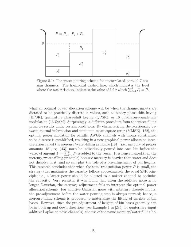
σ21
σ22
σ23
σ24
P1
θP2
P4
P = P1 + P2 + P4
Figure 5.1: The water-pouring scheme for uncorrelated parallel Gaus-sian channels. The horizontal dashed line, which indicates the levelwhere the water rises to, indicates the value of θ for which
∑ki=1 Pi = P .
what an optimal power allocation scheme will be when the channel inputs aredictated to be practically discrete in values, such as binary phase-shift keying(BPSK), quadrature phase-shift keying (QPSK), or 16 quadrature-amplitudemodulation (16-QAM). Surprisingly, a different procedure from the water-fillingprinciple results under certain conditions. By characterizing the relationship be-tween mutual information and minimum mean square error (MMSE) [122], theoptimal power allocation for parallel AWGN channels with inputs constrainedto be discrete is established, resulting in a new graphical power allocation inter-pretation called the mercury/water-filling principle [181]: i.e., mercury of properamounts [181, eq. (43)] must be individually poured into each bin before thewater of amount P =
∑ki=1 Pi is added to the vessel. It is hence named (i.e., the
mercury/water-filling principle) because mercury is heavier than water and doesnot dissolve in it, and so can play the role of a pre-adjustment of bin heights.This research concludes that when the total transmission power P is small, thestrategy that maximizes the capacity follows approximately the equal SNR prin-ciple, i.e., a larger power should be allotted to a noisier channel to optimizethe capacity. Very recently, it was found that when the additive noise is nolonger Gaussian, the mercury adjustment fails to interpret the optimal powerallocation scheme. For additive Gaussian noise with arbitrary discrete inputs,the pre-adjustment before the water pouring step is always upward; hence, amercury-filling scheme is proposed to materialize the lifting of heights of binbases. However, since the pre-adjustment of heights of bin bases generally canbe in both up and down directions (see Example 1 in [284] for quaternary-inputadditive Laplacian noise channels), the use of the name mercury/water filling be-
195

comes inappropriate. For this reason, the graphical interpretation of the optimalpower allocation principle is simply named two-phase water-filling principle in[284]. We end this observation by emphasizing that the true measure for a digitalcommunication system is of no doubt the effective transmission rate subject toan acceptably good transmission error (e.g., an overall bit error rate ≤ 10−5). Inorder to make the analysis tractable, researchers adopt the channel capacity asthe design criterion instead, in the hope of obtaining a simple reference schemefor practical systems. Further study is thus required to examine the feasibil-ity of such an approach (even though the water-filling principle is certainly atheoretically interesting result).
5.6 Capacity of correlated parallel Gaussian channels
In the previous section, we considered a network of k parallel discrete-time mem-oryless Gaussian channels in which the noise samples from different channels areindependent from each other. We found out that the power allocation strat-egy that maximizes the system’s capacity is given by the water-filling scheme.We next study a network of k parallel memoryless Gaussian channels where thenoise variables from different channels are correlated. Surprisingly, we obtainthat water-filling provides also the optimal power allotment policy.
Let KZ denote the covariance matrix of the noise tuple (Z1, Z2, . . . , Zk), andlet KX denote the covariance matrix of the system input (X1, . . . , Xk), where weassume (without loss of the generality) that each Xi has zero mean. We assumethat KZ is positive definite. The input power constraint becomes
k∑
i=1
E[X2i ] = tr(KX) ≤ P,
where tr(·) denotes the trace of the k×k matrix KX . Since in each channel, theinput and noise variables are independent from each other, we have
I(Xk; Y k) = h(Y k) − h(Y k|Xk)
= h(Y k) − h(Zk + Xk|Xk)
= h(Y k) − h(Zk|Xk)
= h(Y k) − h(Zk).
Since h(Zk) is not determined by the input, determining the system’s capacityreduces to maximizing h(Y k) over all possible inputs (X1, . . . , Xk) satisfying thepower constraint.
Now observe that the covariance matrix of Y k is equal to KY = KX + KZ ,which implies by Theorem 5.20 that the differential entropy of Y k is upper
196

bounded by
h(Y k) ≤ 1
2log2
[(2πe)kdet(KX + KZ)
],
with equality iff Y k Gaussian. It remains to find out whether we can find in-puts (X1, . . . , Xk) satisfying the power constraint which achieve the above upperbound and maximize it.
As in the proof of Theorem 5.18, we can orthogonally diagonalize KZ as
KZ = AΛAT ,
where AAT = Ik (and thus det(A)2 = 1), Ik is the k × k identity matrix,and Λ is a diagonal matrix with positive diagonal components consisting of theeigenvalues of KZ (as KZ is positive definite). Then
det(KX + KZ) = det(KX + AΛAT )
= det(AATKXAAT + AΛAT )
= det(A) · det(ATKXA + Λ) · det(AT )
= det(ATKXA + Λ)
= det(B + Λ),
where B , ATKXA. Since for any two matrices C and D, tr(CD) = tr(DC),we have that
tr(B) = tr(ATKXA) = tr(AATKX) = tr(IkKX) = tr(KX).
Thus the capacity problem is further transformed to maximizing det(B + Λ)subject to tr(B) ≤ P .
By observing that B + Λ is positive definite (because Λ is positive definite)and using Hadamard’s inequality given in Corollary 5.19, we have
det(B + Λ) ≤k∏
i=1
(Bii + λi),
where λi is the component of matrix Λ locating at ith row and ith column, whichis exactly the i-th eigenvalue of KZ . Thus, the maximum value of det(B + Λ)under tr(B) ≤ P is realized by a diagonal matrix B (to achieve equality inHadamard’s inequality) with
k∑
i=1
Bii = P.
Finally, as in the proof of Theorem 5.36, we obtain a water-filling allotment forthe optimal diagonal elements of B:
Bii = max0, θ − λi,
197

where θ is chosen to satisfy∑k
i=1 Bii = P . We summarize this result in the nexttheorem.
Theorem 5.38 (Capacity of correlated parallel Gaussian channels) Thecapacity of k correlated parallel Gaussian channels with positive-definite noisecovariance matrix KZ under overall input power constraint P is given by
C(P ) =k∑
i=1
1
2log2
(
1 +Pi
λi
)
,
where λi is the i-th eigenvalue of KZ ,
Pi = max0, θ − λi,
and θ is chosen to satisfy∑k
i=1 Pi = P . This capacity is achieved by a tuple ofzero-mean Gaussian inputs (X1, X2, · · · , Xk) with covariance matrix KX havingthe same eigenvectors as KZ , where the i-th eigenvalue of KX is Pi, for i =1, 2, · · · , k.
5.7 Non-Gaussian discrete-time memoryless channels
If a discrete-time channel has an additive but non-Gaussian memoryless noiseand an input power constraint, then it is often hard to calculate its capacity.Hence, in this section, we introduce an upper bound and a lower bound on thecapacity of such a channel (we assume that the noise admits a pdf).
Definition 5.39 (Entropy power) For a continuous random variable Z with(well-defined) differential entropy h(Z) (measured in bits), its entropy power isdenoted by Ze and defined as
Ze ,1
2πe22·h(Z).
Lemma 5.40 For a discrete-time continuous-alphabet memoryless additive-noisechannel with input power constraint P and noise variance σ2, its capacity satis-fies
1
2log2
P + σ2
Ze
≥ C(P ) ≥ 1
2log2
P + σ2
σ2. (5.7.1)
Proof: The lower bound in (5.7.1) is already proved in Theorem 5.33. The upperbound follows from
I(X; Y ) = h(Y ) − h(Z)
198

≤ 1
2log2[2πe(P + σ2)] − 1
2log2[2πeZe].
2
The entropy power of Z can be viewed as the variance of a correspondingGaussian random variable with the same differential entropy as Z. Indeed, if Zis Gaussian, then its entropy power is equal to
Ze =1
2πe22h(Z) = Var(Z),
as expected.
Whenever two independent Gaussian random variables, Z1 and Z2, are added,the power (variance) of the sum is equal to the sum of the powers (variances) ofZ1 and Z2. This relationship can then be written as
22h(Z1+Z2) = 22h(Z1) + 22h(Z2),
or equivalentlyVar(Z1 + Z2) = Var(Z1) + Var(Z2).
However, when two independent random variables are non-Gaussian, the rela-tionship becomes
22h(Z1+Z2) ≥ 22h(Z1) + 22h(Z2), (5.7.2)
or equivalentlyZe(Z1 + Z2) ≥ Ze(Z1) + Ze(Z2). (5.7.3)
Inequality (5.7.2) (or equivalently (5.7.3)), whose proof can be found in [57,Section 17.8] or [35, Theorem 7.10.4], is called the entropy-power inequality. Itreveals that the sum of two independent random variables may introduce moreentropy power than the sum of each individual entropy power, except in theGaussian case.
Observation 5.41 (Capacity bounds in terms of Gaussian capacity andnon-Gaussianness) It can be readily verified that
1
2log2
P + σ2
Ze
=1
2log2
P + σ2
σ2+ D(Z‖ZG)
where D(Z‖ZG) is the divergence between Z and a Gaussian random variableZG of mean zero and variance σ2. Note that D(Z‖ZG) is called the non-Gaussianness of Z (e.g, see [273]) and is a measure of the “non-Gaussianity”of the noise Z. Thus recalling from (5.4.18)
CG(P ) ,1
2log2
P + σ2
σ2
as the capacity of the channel when the additive noise is Gaussian, we obtainthe following equivalent form for (5.7.1):
CG(P ) + D(Z‖ZG) ≥ C(P ) ≥ CG(P ). (5.7.4)
199

5.8 Capacity of the band-limited white Gaussian channel
We have so far considered discrete-time channels (with discrete or continuousalphabets). We close this chapter by briefly presenting the capacity expressionof the continuous-time (waveform) band-limited channel with additive whiteGaussian noise. The reader is referred to [292], [97, Chapter 8], [19, Sections 8.2and 8.3] and [144, Chapter 6] for rigorous and detailed treatments (includingcoding theorems) of waveform channels.
The continuous-time band-limited channel with additive white Gaussian noiseis a common model for a radio network or a telephone line. For such a channel,illustrated in Figure 5.2, the output waveform is given by
Y (t) = (X(t) + Z(t)) ∗ h(t), t ≥ 0,
where “∗” represents the convolution operation (recall that the convolution be-tween two signals a(t) and b(t) is defined as a(t) ∗ b(t) =
∫∞−∞ a(τ)b(t − τ)dτ).
Here X(t) is the channel input waveform with average power constraint
limT→∞
1
T
∫ T/2
−T/2
E[X2(t)]dt ≤ P (5.8.1)
and bandwidth W cycles per second or Hertz (Hz); i.e., its spectrum or Fouriertransform X(f) , F [X(t)] =
∫ +∞−∞ X(t)e−j2πftdt = 0 for all frequencies |f | > W ,
where j =√−1 is the imaginary unit number. Z(t) is the noise waveform of a
zero-mean stationary white Gaussian process with power spectral density N0/2;i.e., its power spectral density PSDZ(f), which is the Fourier transform of theprocess covariance (equivalently, correlation) function KZ(τ) , E[Z(s)Z(s+τ)],s, τ ∈ R, is given by
PSDZ(f) = F [KZ(t)] =
∫ +∞
−∞KZ(t)e−j2πftdt =
N0
2∀f.
Finally, h(t) is the impulse response of an ideal bandpass filter with cutoff fre-quencies at ±W Hz:
H(f) = F [(h(t)] =
1 if −W ≤ f ≤ W ,
0 otherwise.
Recall that one can recover h(t) by taking the inverse Fourier transform of H(f);this yields
h(t) = F−1[H(f)] =
∫ +∞
−∞H(f)ej2πftdf = 2W sinc(2Wt),
200
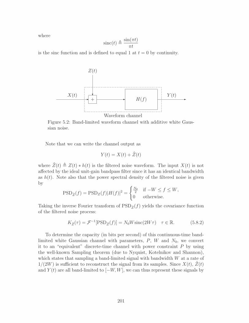
where
sinc(t) ,sin(πt)
πt
is the sinc function and is defined to equal 1 at t = 0 by continuity.
-X(t)
H(f)-+?
Waveform channel
Z(t)
-Y (t)
Figure 5.2: Band-limited waveform channel with additive white Gaus-sian noise.
Note that we can write the channel output as
Y (t) = X(t) + Z(t)
where Z(t) , Z(t) ∗ h(t) is the filtered noise waveform. The input X(t) is notaffected by the ideal unit-gain bandpass filter since it has an identical bandwidthas h(t). Note also that the power spectral density of the filtered noise is givenby
PSDZ(f) = PSDZ(f)|H(f)|2 =
N0
2if −W ≤ f ≤ W ,
0 otherwise.
Taking the inverse Fourier transform of PSDZ(f) yields the covariance functionof the filtered noise process:
KZ(τ) = F−1[PSDZ(f)] = N0W sinc(2Wτ) τ ∈ R. (5.8.2)
To determine the capacity (in bits per second) of this continuous-time band-limited white Gaussian channel with parameters, P , W and N0, we convertit to an “equivalent” discrete-time channel with power constraint P by usingthe well-known Sampling theorem (due to Nyquist, Kotelnikov and Shannon),which states that sampling a band-limited signal with bandwidth W at a rate of1/(2W ) is sufficient to reconstruct the signal from its samples. Since X(t), Z(t)and Y (t) are all band-limited to [−W,W ], we can thus represent these signals by
201

their samples taken 12W
seconds apart and model the channel by a discrete-timechannel described by:
Yn = Xn + Zn, n = 0,±1,±2, · · · ,
where Xn , X( n2W
) are the input samples and Zn = Z( n2W
) and Yn = Y ( n2W
)
are the random samples of the noise Z(t) and output Y (t) signals, respectively.
Since Z(t) is a filtered version of Z(t), which is a zero-mean stationary Gaus-sian process, we obtain that Z(t) is also zero-mean, stationary and Gaussian.This directly implies that the samples Zn, n = 1, 2, · · · , are zero-mean Gaussianidentically distributed random variables. Now an examination of the expressionof KZ(τ) in (5.8.2) reveals that
KZ(τ) = 0
for τ = n2W
, n = 1, 2, · · · , since sinc(t) = 0 for all non-zero integer values
of t. Hence, the random variables Zn, n = 1, 2, · · · , are uncorrelated and henceindependent (since they are Gaussian) and their variance is given by E[Z2
n] =KZ(0) = N0W . We conclude that the discrete-time process Zn∞n=1 is i.i.d.Gaussian with each Zn ∼ N (0, N0W ). As a result, the above discrete-timechannel is a discrete-time memoryless Gaussian channel with power constraintP and noise variance N0W ; thus the capacity of the band-limited white Gaussianchannel in bits per channel use is given using (5.4.13) by
1
2log2
(
1 +P
N0W
)
bits/channel use.
Given that we are using the channel (with inputs Xn) every 12W
seconds, we ob-tain that the capacity in bits/second of the band-limited white Gaussian channelis given by
C(P ) = W log2
(
1 +P
N0W
)
bits/second, (5.8.3)
where PN0W
is the channel SNR.12
12Note that (5.8.3) is achieved by zero-mean i.i.d. Gaussian Xn∞n=−∞ with E[X2n] = P ,
which can be obtained by sampling a zero-mean, stationary and Gaussian X(t) with
PSDX(f) =
P
2W if −W ≤ f ≤ W ,
0 otherwise.
Examining this X(t) confirms that it satisfies (5.8.1):
1
T
∫ T/2
−T/2
E[X2(t)]dt = E[X2(t)] = KX(0) = P · sinc(2W · 0) = P.
202

We emphasize that the above derivation of (5.8.3) is heuristic as we have notrigorously shown the equivalence between the original band-limited Gaussianchannel and its discrete-time version and we have not established a coding the-orem for the original channel. We point the reader to the references mentionedat the beginning of the section for a full development of this subject.
Example 5.42 (Telephone line channel) Suppose telephone signals are band-limited to 4 kHz. Given an SNR of 40 decibels (dB), i.e.,
10 log10
P
N0W= 40 dB,
then from (5.8.3), we calculate that the capacity of the telephone line channel(when modeled via the band-limited white Gaussian channel) is given by
4000 log2(1 + 10000) = 53151.4 bits/second.
Example 5.43 (Infinite bandwidth white Gaussian channel) As the chan-nel bandwidth W grows without bound, we obtain from (5.8.3) that
limW→∞
C(P ) =P
N0
log2 e bits/second,
which indicates that in the infinite-bandwidth regime, capacity grows linearlywith power.
Observation 5.44 (Band-limited colored Gaussian channel) If the aboveband-limited channel has a stationary colored (non-white) additive Gaussiannoise, then it can be shown (e.g., see [97]) that the capacity of this channelbecomes
C(P ) =1
2
∫ W
−W
max
[
0, log2
θ
PSDZ(f)
]
df,
where θ is the solution of
P =
∫ W
−W
max [0, θ − PSDZ(f)] df.
The above capacity formula is indeed reminiscent of the water-pouring scheme wesaw in Sections 5.5 and 5.6, albeit it is herein applied in the spectral domain. Inother words, we can view the curve of PSDZ(f) as a bowl, and water is imaginedbeing poured into the bowl up to level θ under which the area of the water isequal to P (see Figure 5.3.(a)). Furthermore, the distributed water indicates theshape of the optimum transmission power spectrum (see Figure 5.3.(b)).
203
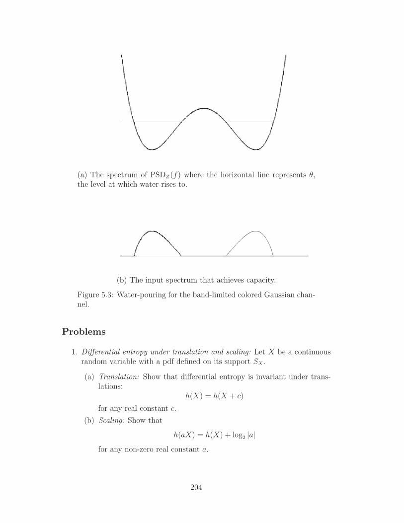
(a) The spectrum of PSDZ(f) where the horizontal line represents θ,the level at which water rises to.
(b) The input spectrum that achieves capacity.
Figure 5.3: Water-pouring for the band-limited colored Gaussian chan-nel.
Problems
1. Differential entropy under translation and scaling: Let X be a continuousrandom variable with a pdf defined on its support SX .
(a) Translation: Show that differential entropy is invariant under trans-lations:
h(X) = h(X + c)
for any real constant c.
(b) Scaling: Show that
h(aX) = h(X) + log2 |a|for any non-zero real constant a.
204

2. Determine the differential entropy (in nats) of random variable X for eachof the following cases.
(a) X is exponential with parameter λ > 0 and pdf fX(x) = λe−λx, x ≥ 0.
(b) X is Laplacian with parameter λ > 0, mean zero and pdf fX(x) =12λ
e−|x|λ , x ∈ R.
(c) X is log-normal with parameters µ ∈ R and σ > 0; i.e., X = eY ,where Y ∼ N (µ, σ2) is a Gaussian random variable with mean µ andvariance σ2. The pdf of X is given by
fX(x) =1
σx√
2πe−
(ln x−µ)2
2σ2 , x > 0.
(d) The source X = aX1 + bX2, where a and b are non-zero constantsand X1 and X2 are independent Gaussian random variables such thatX1 ∼ N (µ1, σ
21) and X2 ∼ N (µ2, σ
22).
3. Generalized Gaussian: Let X be a generalized Gaussian random variablewith mean zero, variance σ2 and pdf given by
fX(x) =αη
2Γ( 1α)e−ηα|x|α , x ∈ R
where α > 0 is a parameter describing the distribution’s exponential rateof decay,
η = σ−1
[Γ( 3
α)
Γ( 1α)
]1/2
and
Γ(x) =
∫ ∞
0
tx−1e−tdt, x > 0,
is the gamma function (recall that Γ(1/2) =√
π, Γ(1) = 1 and that Γ(x +1) = xΓ(x) for any positive x.) The generalized Gaussian distribution(also called the exponential power distribution) is well-known to providea good model for symmetrically distributed random processes, includingimage wavelet transform coefficients [185] and broad-tailed processes suchas atmospheric impulsive noise [13]. Note that when α = 2, fX reducesto the Gaussian pdf with mean zero and variance σ2, and when α = 1, itreduces to the Laplacian pdf with parameter σ/
√2 (i.e., variance σ2).
(a) Show that the differential entropy of X is given by
h(X) =1
α+ ln
(2Γ( 1
α)
αη
)
(in nats).
205

(b) Show that when α = 2 and α = 1, h(X) reduces to the differentialentropy of the Gaussian and Laplacian distributions, respectively.
4. Prove that, of all pdfs with support [0, 1], the uniform density function hasthe largest differential entropy.
5. Of all pdfs with continuous support [0, K], where K > 1 is finite, whichpdf has the largest differential entropy?
Hint: If fX is the pdf that maximizes differential entropy among all pdfswith support [0, K], then E[log fX(X)] = E[log fX(Y )] for any randomvariable Y of support [0, K].
6. Show that the exponential distribution has the largest differential entropyamong all pdfs with mean µ and support [0,∞). (Recall that the pdf ofthe exponential distribution with mean µ is given by fX(x) = 1
µexp(−x
µ)
for x ≥ 0.)
7. Show that among all continuous random variables X admitting a pdf withsupport R and finite differential entropy and satisfying E[X] = 0 andE[|X|] = λ, where λ > 0 is a fixed parameter, the Laplacian randomvariable with pdf
fX(x) =1
2λe−
|x|λ for x ∈ R
maximizes differential entropy.
8. Find the mutual information between the dependent Gaussian zero-meanrandom variables X and Y with covariance matrix
(σ2 ρσ2
ρσ2 σ2
)
where ρ ∈ [−1, 1] is the correlation coefficient. Evaluate the value ofI(X; Y ) when ρ = 1, ρ = 0 and ρ = −1, and explain the results.
9. A variant of the fundamental inequality for the logarithm: For any x > 0and y > 0, show that
y ln(y
x
)
≥ y − x
with equality iff x = y.
10. Non-negativity of divergence: Let X and Y be two continuous randomvariables with pdfs fX and fY , respectively, such that their supports satisfySX ⊆ SY ⊆ R. Use Problem 4.9 to show that
D(fX‖fY ) ≥ 0
with equality iff fX = fY almost everywhere.
206

11. Divergence between Laplacians: Let S be a random variable admitting apdf with support R with mean zero and satisfying E[|S|] = λ, where λ > 0is a fixed parameter.
(a) Let fS and gS be two zero-mean Laplacian pdfs for S with parametersλ and λ, respectively (see Problem 7 above for the Laplacian pdfexpression). Determine D(fS‖gS) in nats in terms of λ and λ.
(b) Show that for any valid pdf f for S, we have
D(f‖gS) ≥ D(fS‖gS)
with equality iff f = fS (almost everywhere).
12. Let X, Y , and Z be jointly Gaussian random variables, each with mean 0and variance 1; let the correlation coefficient of X and Y as well as that ofY and Z be ρ, while X and Z are uncorrelated. Determine h(X,Y, Z).
13. Let random variables Z1 and Z2 have Gaussian joint distribution withE[Z1] = E[Z2] = 0, E[Z2
1 ] = E[Z22 ] = 1 and E[Z1Z2] = ρ, where 0 < ρ < 1.
Also, let U be a uniformly distributed random variable over the interval(0, 2πe). Determine whether or not the following inequality holds:
h(U) > h(Z1, Z2 − 3Z1).
14. Let Z1 and Z2 be two independent continuous random variables with iden-tical pdfs. Show that [35]
I(Z1; Z1 + Z2) ≥1
2(in bits.).
Hint: Use the entropy-power inequality in (5.7.2).
15. An alternative form of the entropy-power inequality: Show that the entropy-power inequality in (5.7.2) can be written as
h(Z1 + Z2) ≥ h(Y1 + Y2)
where Z1 and Z2 are two independent continuous random variables, andY1 and Y2 are two independent Gaussian random variables such that
h(Y1) = h(Z1)
andh(Y2) = h(Z2).
207

16. Estimation error and differential entropy: Consider a continuous randomvariable Z with a pdf.
(a) Let Z be an estimate of Z based on only the knowledge of the distri-bution of Z. Show that the mean-square estimation error satisfies
E[(Z − Z)2] ≥ 22h(Z)
2πe
with equality iff Z is Gaussian and Z = E[Z].
Hint: Recall that Z∗ = E[Z] is the optimal (MMSE) estimate of Z.
(b) Assume now that the estimator has access to observation Y , which iscorrelated to Z (such that their joint and conditional pdfs are well-defined), thus giving estimate Z = Z(Y ). Show that
E[(Z − Z(Y ))2] ≥ 22h(Z|Y )
2πe
with equality iff Z is Gaussian and Z = E[Z|Y ].
17. Consider three continuous real-valued random variables X, Y1 and Y2 ad-mitting a joint pdf and conditional pdfs among them such that Y1 andY2 are conditionally independent and conditionally identical distributedgiven X.
(a) Show I(X; Y1, Y2) = 2 · I(X; Y1) − I(Y1; Y2).
(b) Show that the capacity of the channel X → (Y1, Y2) with input powerconstraint P is less than twice the capacity of the channel X → Y1.
18. Consider the channel X → (Y1, Y2) with
Y1 = X + Z1 and Y2 = X + Z2.
Assume Z1 and Z2 are zero-mean dependent Gaussian random variableswith covariance matrix (
N NρNρ N
)
.
By applying a power constraint on the input, i.e., E[X2] ≤ S. Find thechannel’s capacity for the following values of ρ:
(a) ρ = 1;
(b) ρ = 0;
(c) ρ = −1.
208
19. Consider a continuous-alphabet channel with a vectored output for a scalarinput as follows.
X → Channel → Y1, Y2
Suppose that the channel’s transition pdf satisfies
fY1,Y2|X(y1, y2|x) = fY1|X(y1|x)fY2|X(y2|x)
for every y1, y2 and x.
(a) Show that I(X; Y1, Y2) =(∑2
i=1 I(X; Yi))− I(Y1; Y2).
Hint: I(X; Y1, Y2) = h(Y1, Y2) − h(Y1|X) − h(Y2|X).
(b) Prove that the channel capacity Ctwo(S) of using two outputs (Y1, Y2)is less than C1(S) + C2(S) under an input power constraint S, whereCj(S) is the channel capacity of using one output Yj and ignoring theother output.
(c) Further assume that fYi|X(·|x) is Gaussian with mean x and varianceσ2
j . In fact, these channels can be expressed as Y1 = X + N1 andY2 = X + N2, where (N1, N2) are independent Gaussian distributed
with mean zero and covariance matrix
[σ2
1 00 σ2
2
]
. Using the fact that
h(Y1, Y2) ≤ 12log(2πe)2 |KY1,Y2 | with equality holding when (Y1, Y2)
are joint Gaussian, where KY1,Y2 is the covariance matrix of (Y1, Y2),derive Ctwo(S) for the two-output channel under the power constraintE[X2] ≤ S.
Hint: I(X; Y1, Y2) = h(Y1, Y2)−h(N1, N2) = h(Y1, Y2)−h(N1)−h(N2).
20. Consider the 3-input 3-output memoryless additive Gaussian channel
Y = X + Z,
where X = [X1, X2, X3], Y = [Y1, Y2, Y3] and Z = [Z1, Z2, Z3] are all 3-Dimensional real vectors. Assume that X is independent of Z, and theinput power constraint is S (i.e., E(X2
1 + X22 + X2
3 ) ≤ S). Also, assumethat Z is Gaussian distributed with zero mean and covariance matrix K,where
K =
1 0 00 1 ρ0 ρ 1
.
(a) Determine the capacity-cost function of the channel, if ρ = 0.
Hint: Directly apply Theorem 5.36.
(b) Determine the capacity-cost function of the channel, if 0 < ρ < 1.
Hint: Directly apply Theorem 5.38.
209

Chapter 6
Lossy Data Compression andTransmission
6.1 Preliminaries
6.1.1 Motivation
In a number of situations, one may need to compress a source to a rate lessthan the source entropy, which as we saw in Chapter 3 is the minimum losslessdata compression rate. In this case, some sort of data loss is inevitable and theresultant code is referred to as a lossy data compression code. The following areexamples for requiring the use of lossy data compression.
Example 6.1 (Digitization or quantization of continuous signals) Theinformation content of continuous-alphabet signals, such as voice or analog im-ages, is typically infinite, requiring an unbounded number of bits to digitizethem without incurring any loss, which is not feasible. Therefore, a lossy datacompression code must be used to reduce the output of a continuous source toa finite number of bits.
Example 6.2 (Extracting useful information) In some scenarios, the sourceinformation may not be operationally useful in its entirety. A quick example isthe hypothesis testing problem where the system designer is only concerned withknowing the likelihood ratio of the null hypothesis distribution against the al-ternative hypothesis distribution (see Chapter 2). Therefore, any two distinctsource letters which produce the same likelihood ratio are not encoded into dis-tinct codewords and the resultant code is lossy.
Example 6.3 (Channel capacity bottleneck) Transmitting at a rate of rsource symbol/channel symbol a discrete (memoryless) source with entropy H
210
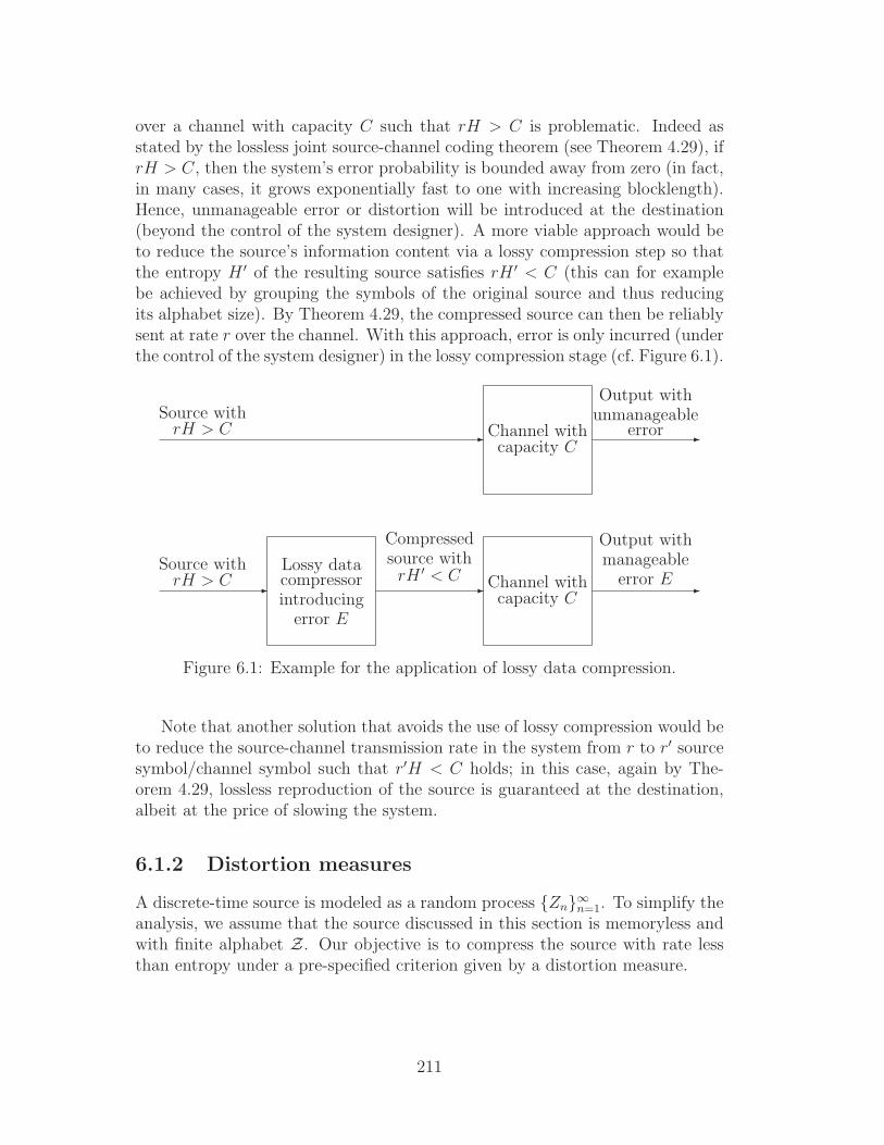
over a channel with capacity C such that rH > C is problematic. Indeed asstated by the lossless joint source-channel coding theorem (see Theorem 4.29), ifrH > C, then the system’s error probability is bounded away from zero (in fact,in many cases, it grows exponentially fast to one with increasing blocklength).Hence, unmanageable error or distortion will be introduced at the destination(beyond the control of the system designer). A more viable approach would beto reduce the source’s information content via a lossy compression step so thatthe entropy H ′ of the resulting source satisfies rH ′ < C (this can for examplebe achieved by grouping the symbols of the original source and thus reducingits alphabet size). By Theorem 4.29, the compressed source can then be reliablysent at rate r over the channel. With this approach, error is only incurred (underthe control of the system designer) in the lossy compression stage (cf. Figure 6.1).
- Channel withcapacity C
-
Source withrH > C
Output withunmanageable
error
-
Lossy datacompressorintroducing
error E
-
Compressedsource withrH ′ < C Channel with
capacity C-
Source withrH > C
Output withmanageable
error E
Figure 6.1: Example for the application of lossy data compression.
Note that another solution that avoids the use of lossy compression would beto reduce the source-channel transmission rate in the system from r to r′ sourcesymbol/channel symbol such that r′H < C holds; in this case, again by The-orem 4.29, lossless reproduction of the source is guaranteed at the destination,albeit at the price of slowing the system.
6.1.2 Distortion measures
A discrete-time source is modeled as a random process Zn∞n=1. To simplify theanalysis, we assume that the source discussed in this section is memoryless andwith finite alphabet Z. Our objective is to compress the source with rate lessthan entropy under a pre-specified criterion given by a distortion measure.
211
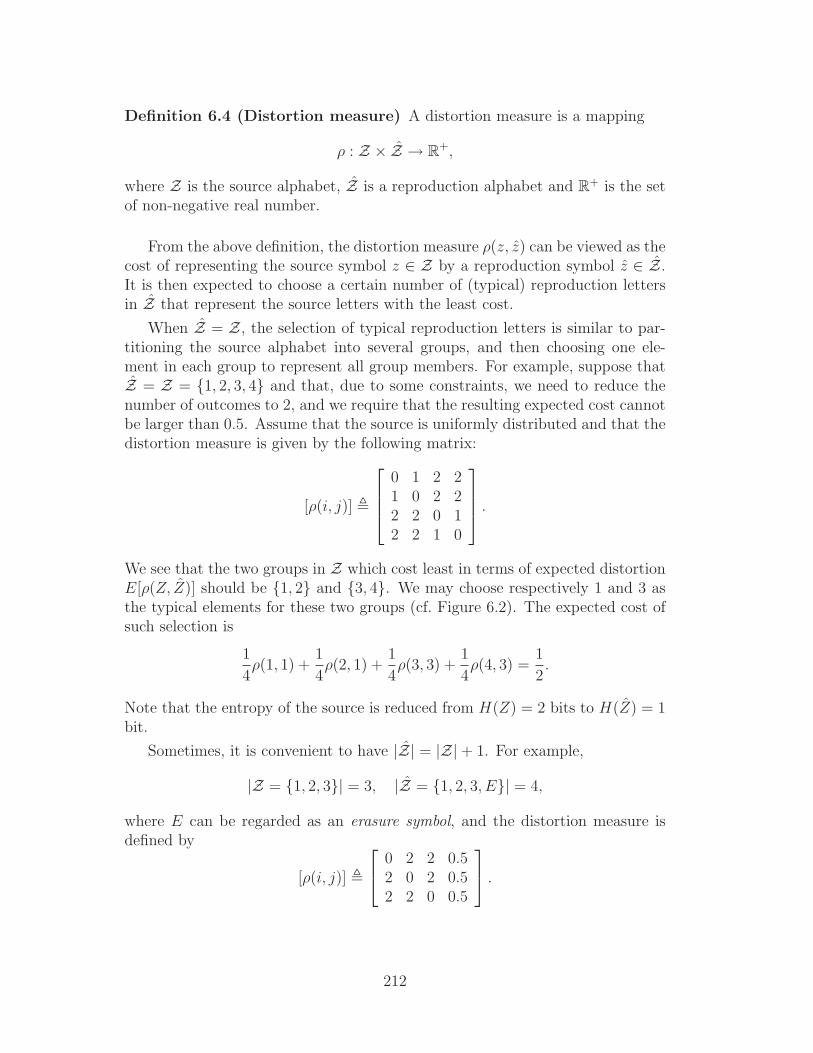
Definition 6.4 (Distortion measure) A distortion measure is a mapping
ρ : Z × Z → R+,
where Z is the source alphabet, Z is a reproduction alphabet and R+ is the setof non-negative real number.
From the above definition, the distortion measure ρ(z, z) can be viewed as thecost of representing the source symbol z ∈ Z by a reproduction symbol z ∈ Z.It is then expected to choose a certain number of (typical) reproduction lettersin Z that represent the source letters with the least cost.
When Z = Z, the selection of typical reproduction letters is similar to par-titioning the source alphabet into several groups, and then choosing one ele-ment in each group to represent all group members. For example, suppose thatZ = Z = 1, 2, 3, 4 and that, due to some constraints, we need to reduce thenumber of outcomes to 2, and we require that the resulting expected cost cannotbe larger than 0.5. Assume that the source is uniformly distributed and that thedistortion measure is given by the following matrix:
[ρ(i, j)] ,
0 1 2 21 0 2 22 2 0 12 2 1 0
.
We see that the two groups in Z which cost least in terms of expected distortionE[ρ(Z, Z)] should be 1, 2 and 3, 4. We may choose respectively 1 and 3 asthe typical elements for these two groups (cf. Figure 6.2). The expected cost ofsuch selection is
1
4ρ(1, 1) +
1
4ρ(2, 1) +
1
4ρ(3, 3) +
1
4ρ(4, 3) =
1
2.
Note that the entropy of the source is reduced from H(Z) = 2 bits to H(Z) = 1bit.
Sometimes, it is convenient to have |Z| = |Z| + 1. For example,
|Z = 1, 2, 3| = 3, |Z = 1, 2, 3, E| = 4,
where E can be regarded as an erasure symbol, and the distortion measure isdefined by
[ρ(i, j)] ,
0 2 2 0.52 0 2 0.52 2 0 0.5
.
212

1
3
2
4
⇒1?
Representative for group 1, 2
3
Representative for group 3, 4
6
2
4
Figure 6.2: “Grouping” as a form of lossy data compression.
In this case, assume again that the source is uniformly distributed and that torepresent source letters by distinct letters in 1, 2, 3 will yield four times the costincurred when representing them by E. Therefore, if only 2 outcomes are allowed,and the expected distortion cannot be greater than 1/3, then employing typicalelements 1 and E to represent groups 1 and 2, 3, respectively, is an optimalchoice. The resultant entropy is reduced from log2(3) bits to [log2(3)−2/3] bits.It needs to be pointed out that having |Z| > |Z|+1 is usually not advantageous.
6.1.3 Frequently used distortion measures
Example 6.5 (Hamming distortion measure) Let the source and reproduc-tion alphabets be identical, i.e., Z = Z. Then the Hamming distortion measureis given by
ρ(z, z) ,
0, if z = z;1, if z 6= z.
It is also named the probability-of-error distortion measure because
E[ρ(Z, Z)] = Pr(Z 6= Z).
Example 6.6 (Absolute error distortion measure) Assuming that Z = Z,the absolute error distortion measure is given by
ρ(z, z) , |z − z|.
Example 6.7 (Squared error distortion measure) Again assuming that Z =Z, the squared error distortion measure is given by
ρ(z, z) , (z − z)2.
The squared error distortion measure is perhaps the most popular distortionmeasure used for continuous alphabets.
213

Note that all above distortion measures belong to the class of so-called dif-ference distortion measures, which have the form ρ(z, z) = d(x − x) for somenon-negative function d(·, ·). The squared error distortion measure has the ad-vantages of simplicity and having a closed-form solution for most cases of interest,such as when using least squares prediction. Yet, this measure is not ideal forpractical situations involving data operated by human observers (such as imageand speech data) as it is inadequate in measuring perceptual quality. For ex-ample, two speech waveforms in which one is a marginally time-shifted versionof the other may have large square error distortion; however, they sound quitesimilar to the human ear.
The above definition for distortion measures can be viewed as a single-letterdistortion measure since they consider only one random variable Z which drawsa single letter. For sources modeled as a sequence of random variables Zn,some extension needs to be made. A straightforward extension is the additivedistortion measure.
Definition 6.8 (Additive distortion measure between vectors) The ad-ditive distortion measure ρn between vectors zn and zn of size n (or n-sequencesor n-tuples) is defined by
ρn(zn, zn) =n∑
i=1
ρ(zi, zi).
Another example that is also based on a per-symbol distortion is the maxi-mum distortion measure:
Definition 6.9 (Maximum distortion measure)
ρn(zn, zn) = max1≤i≤n
ρ(zi, zi).
After defining the distortion measures for source sequences, a natural ques-tion to ask is whether to reproduce source sequence zn by sequence zn of thesame length is a must or not. To be more precise, can we use zk to representzn for k 6= n? The answer is certainly yes if a distortion measure for zn andzk is defined. A quick example will be that the source is a ternary sequenceof length n, while the (fixed-length) data compression result is a set of binaryindices of length k, which is taken as small as possible subject to some givenconstraints. Hence, k is not necessarily equal to n. One of the problems for tak-ing k 6= n is that the distortion measure for sequences can no longer be definedbased on per-letter distortions, and hence a per-letter formula for the best lossydata compression rate cannot be rendered.
214

In order to alleviate the aforementioned (k 6= n) problem, we claim that formost cases of interest, it is reasonable to assume k = n. This is because one canactually implement lossy data compression from Zn to Zk in two steps. Thefirst step corresponds to a lossy compression mapping hn : Zn → Zn, and thesecond step performs indexing hn(Zn) into Zk:
Step 1 : Find the data compression mapping
hn : Zn → Zn
for which the pre-specified distortion and rate constraints are satisfied.
Step 2 : Derive the (asymptotically) lossless data compression block code forsource hn(Zn). When n is sufficiently large, the existence of such code withblock length
k > H(hn(Zn))
(
equivalently, R =k
n>
1
nH(hn(Zn)
)
is guaranteed by Shannon’s source coding theorem (Theorem 3.5).
Through the above two steps, a lossy data compression code from
Zn → Zn︸ ︷︷ ︸
Step 1
→ 0, 1k
is established. Since the second step is already discussed in the (asymptotically)lossless data compression context, we can say that the theorem regarding lossydata compression is basically a theorem on the first step.
6.2 Fixed-length lossy data compression codes
Similar to the lossless source coding theorem, the objective is to find the theo-retical limit of the compression rate for lossy source codes. Before introducingthe main theorem, we first formally define lossy data compression codes, therate-distortion region and the (operational) rate-distortion function.
Definition 6.10 (Fixed-length lossy data compression code subject toan average distortion constraint) An (n,M,D) fixed-length lossy data com-pression code for a source Zn with alphabet Z and reproduction alphabet Zconsists of a compression function
h : Zn → Zn
215

with a codebook size (i.e., the image h(Zn)) equal to |h(Zn)| = M = Mn andan average (expected) distortion no larger than distortion threshold D ≥ 0:
E
[1
nρn(Zn, h(Zn))
]
≤ D.
The compression rate of the code is defined as (1/n) log2 M bits/source symbol,as log2 M bits can be used to represent a sourceword of length n. Indeed anequivalent description of the above compression code can be made via an encoder-decoder pair (f, g), where
f : Zn → 1, 2, · · · ,M
is an encoding function mapping each sourceword in Zn to an index in 1, · · · ,M(which can be represented using log2 M bits), and
g : 1, 2, · · · ,M → Zn
is a decoding function mapping each index to a reconstruction (or reproduction)vector in Zn such that the composition of the encoding and decoding functionsyields the above compression function h: g(f(zn)) = h(zn) for zn ∈ Zn.
Definition 6.11 (Achievable rate-distortion pair) For a given source Znand a sequence of distortion measures ρnn≥1, a rate-distortion pair (R,D) isachievable if there exists a sequence of fixed-length lossy data compression codes(n,Mn, D) for the source with ultimate code rate satisfying
lim supn→∞
1
nlog Mn ≤ R.
Definition 6.12 (Rate-distortion region) The rate-distortion region R of asource Zn is the closure of the set of all achievable rate-distortion pair (R,D).
Lemma 6.13 (Time-sharing principle) Under an additive distortion mea-sure ρn, the rate-distortion region R is a convex set; i.e., if (R1, D1) ∈ R and(R2, D2) ∈ R, then (λR1 + (1 − λ)R2, λD1 + (1 − λ)D2) ∈ R for all 0 ≤ λ ≤ 1.
Proof: It is enough to show that the set of all achievable rate-distortion pairsis convex (since the closure of a convex set is convex). Also, assume without lossof generality that 0 < λ < 1.
We will prove convexity of the set of all achievable rate-distortion pairs byusing a time-sharing argument, which basically states that if we can use an(n,M1, D1) code C∼1 to achieve (R1, D1) and an (n,M2, D2) code C∼2 to achieve
216

(R2, D2), then for any rational number 0 < λ < 1, we can use C∼1 for a fractionλ of the time and use C∼2 for a fraction 1 − λ of the time to achieve (Rλ, Dλ),where Rλ = λR1 + (1− λ)R2 and Dλ = λD1 + (1− λ)D2; hence the result holdsfor any real number 0 < λ < 1 by the density of the rational numbers in R andthe continuity of Rλ and Dλ in λ.
Let r and s be positive integers and let λ = rr+s
; then 0 < λ < 1. Now assumethat the pairs (R1, D1) and (R2, D2) are achievable. Then for any δ > 0, thereexist a sequence of (n,M1, D1) codes C∼1 and a sequence of (n,M2, D2) codes C∼2
such that for n sufficiently large,
1
nlog2 M1 ≤ R1 + δ
and1
nlog2 M2 ≤ R2 + δ.
Now construct a sequence of new codes C∼ of blocklength nλ = (r+s)n, codebooksize M = M r
1 × M s2 and compression function h : Z(r+s)n → Z(r+s)n such that
h(z(r+s)n) =(h1(z
n1 ), · · · , h1(z
nr ), h2(z
nr+1), · · · , h2(z
nr+s)
)
wherez(r+s)n = (zn
1 , · · · , znr , zn
r+1, · · · , znr+s)
and h1 and h2 are the compression functions of C∼1 and C∼2, respectively. In otherwords, each reconstruction vector h(z(r+s)n) of code C∼ is a concatenation of rreconstruction vectors of code C∼1 and s reconstruction vectors of code C∼2.
The average (or expected) distortion under the additive distortion measureρn and the rate of code C∼ are given by
E
[ρr+s(z
(r+s)n, h(z(r+s)n))
(r + s)n
]
=1
r + s
(
E
[ρn(zn
1 , h1(zn1 ))
n
]
+ · · · + E
[ρn(zn
r , h1(znr ))
n
]
+E
[ρn(zn
r+1, h2(znr+1))
n
]
+ · · · + E
[ρn(zn
r+s, h2(znr+s))
n
])
≤ 1
r + s(rD1 + sD2)
= λD1 + (1 − λ)D2 = Dλ
and
1
(r + s)nlog2 M =
1
(r + s)nlog2(M
r1 × M s
2 )
=r
(r + s)
1
nlog2 M1 +
s
(r + s)
1
nlog2 M2
217
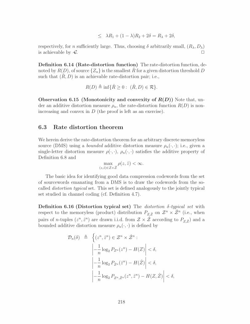
≤ λR1 + (1 − λ)R2 + 2δ = Rλ + 2δ,
respectively, for n sufficiently large. Thus, choosing δ arbitrarily small, (Rλ, Dλ)is achievable by C∼. 2
Definition 6.14 (Rate-distortion function) The rate-distortion function, de-noted by R(D), of source Zn is the smallest R for a given distortion threshold Dsuch that (R,D) is an achievable rate-distortion pair; i.e.,
R(D) , infR ≥ 0 : (R,D) ∈ R.
Observation 6.15 (Monotonicity and convexity of R(D)) Note that, un-der an additive distortion measure ρn, the rate-distortion function R(D) is non-increasing and convex in D (the proof is left as an exercise).
6.3 Rate distortion theorem
We herein derive the rate-distortion theorem for an arbitrary discrete memorylesssource (DMS) using a bounded additive distortion measure ρn(·, ·); i.e., given asingle-letter distortion measure ρ(·, ·), ρn(·, ·) satisfies the additive property ofDefinition 6.8 and
max(z,z)∈Z×Z
ρ(z, z) < ∞.
The basic idea for identifying good data compression codewords from the setof sourcewords emanating from a DMS is to draw the codewords from the so-called distortion typical set. This set is defined analogously to the jointly typicalset studied in channel coding (cf. Definition 4.7).
Definition 6.16 (Distortion typical set) The distortion δ-typical set withrespect to the memoryless (product) distribution PZ,Z on Zn × Zn (i.e., when
pairs of n-tuples (zn, zn) are drawn i.i.d. from Z × Z according to PZ,Z) and abounded additive distortion measure ρn(·, ·) is defined by
Dn(δ) ,
(zn, zn) ∈ Zn × Zn :∣∣∣∣− 1
nlog2 PZn(zn) − H(Z)
∣∣∣∣< δ,
∣∣∣∣− 1
nlog2 PZn(zn) − H(Z)
∣∣∣∣< δ,
∣∣∣∣− 1
nlog2 PZn,Zn(zn, zn) − H(Z, Z)
∣∣∣∣< δ,
218
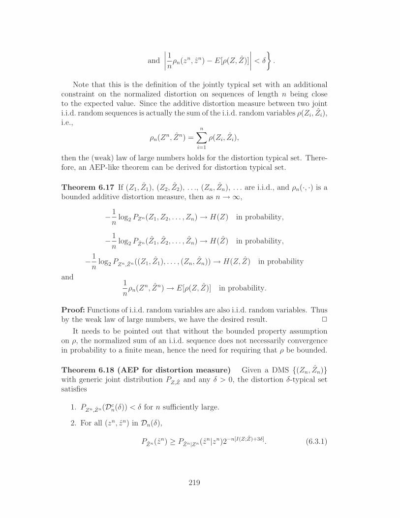
and
∣∣∣∣
1
nρn(zn, zn) − E[ρ(Z, Z)]
∣∣∣∣< δ
.
Note that this is the definition of the jointly typical set with an additionalconstraint on the normalized distortion on sequences of length n being closeto the expected value. Since the additive distortion measure between two jointi.i.d. random sequences is actually the sum of the i.i.d. random variables ρ(Zi, Zi),i.e.,
ρn(Zn, Zn) =n∑
i=1
ρ(Zi, Zi),
then the (weak) law of large numbers holds for the distortion typical set. There-fore, an AEP-like theorem can be derived for distortion typical set.
Theorem 6.17 If (Z1, Z1), (Z2, Z2), . . ., (Zn, Zn), . . . are i.i.d., and ρn(·, ·) is abounded additive distortion measure, then as n → ∞,
− 1
nlog2 PZn(Z1, Z2, . . . , Zn) → H(Z) in probability,
− 1
nlog2 PZn(Z1, Z2, . . . , Zn) → H(Z) in probability,
− 1
nlog2 PZn,Zn((Z1, Z1), . . . , (Zn, Zn)) → H(Z, Z) in probability
and1
nρn(Zn, Zn) → E[ρ(Z, Z)] in probability.
Proof: Functions of i.i.d. random variables are also i.i.d. random variables. Thusby the weak law of large numbers, we have the desired result. 2
It needs to be pointed out that without the bounded property assumptionon ρ, the normalized sum of an i.i.d. sequence does not necessarily convergencein probability to a finite mean, hence the need for requiring that ρ be bounded.
Theorem 6.18 (AEP for distortion measure) Given a DMS (Zn, Zn)with generic joint distribution PZ,Z and any δ > 0, the distortion δ-typical setsatisfies
1. PZn,Zn(Dcn(δ)) < δ for n sufficiently large.
2. For all (zn, zn) in Dn(δ),
PZn(zn) ≥ PZn|Zn(zn|zn)2−n[I(Z;Z)+3δ]. (6.3.1)
219

Proof: The first result follows directly from Theorem 6.17 and the definition ofthe distortion typical set Dn(δ). The second result can be proved as follows:
PZn|Zn(zn|zn) =PZn,Zn(zn, zn)
PZn(zn)
= PZn(zn)PZn,Zn(zn, zn)
PZn(zn)PZn(zn)
≤ PZn(zn)2−n[H(Z,Z)−δ]
2−n[H(Z)+δ]2−n[H(Z)+δ]
= PZn(zn)2n[I(Z;Z)+3δ],
where the inequality follows from the definition of Dn(δ). 2
Before presenting the lossy data compression theorem, we need the followinginequality.
Lemma 6.19 For 0 ≤ x ≤ 1, 0 ≤ y ≤ 1, and n > 0,
(1 − xy)n ≤ 1 − x + e−yn, (6.3.2)
with equality holding iff (x, y) = (1, 0).
Proof: Let gy(t) , (1−yt)n. It can be shown by taking the second derivative ofgy(t) with respect to t that this function is strictly convex for t ∈ [0, 1]. Hence,for any x ∈ [0, 1],
(1 − xy)n = gy
((1 − x) · 0 + x · 1
)
≤ (1 − x) · gy(0) + x · gy(1)
with equality holding iff (x = 0) ∨ (x = 1) ∨ (y = 0)
= (1 − x) + x · (1 − y)n
≤ (1 − x) + x ·(e−y)n
with equality holding iff (x = 0) ∨ (y = 0)
≤ (1 − x) + e−ny
with equality holding iff (x = 1).
From the above derivation, we know that equality holds in (6.3.2) iff
[(x = 0) ∨ (x = 1) ∨ (y = 0)] ∧ [(x = 0) ∨ (y = 0)] ∧ [(x = 1)] = (x = 1, y = 0).
(Note that (x = 0) represents (x, y) ∈ R2 : x = 0 and y ∈ [0, 1]; a similardefinition applies to the other sets.) 2
220

Theorem 6.20 (Rate distortion theorem for memoryless sources) Con-sider a DMS Zn∞n=1 with alphabet Z, reproduction alphabet Z and a boundedadditive distortion measure ρn(·, ·); i.e.,
ρn(zn, zn) =n∑
i=1
ρ(zi, zi) and ρmax , max(z,z)∈Z×Z
ρ(z, z) < ∞,
where ρ(·, ·) is a given single-letter distortion measure. Then the source’s rate-distortion function satisfies the following expression
R(D) = minPZ|Z : E[ρ(Z,Z)]≤D
I(Z; Z).
Proof: DefineR(I)(D) , min
PZ|Z : E[ρ(Z,Z)]≤DI(Z; Z); (6.3.3)
this quantity is typically called Shannon’s information rate-distortion function.We will then show that the (operational) rate-distortion function R(D) given inDefinition 6.14 equals R(I)(D).
1. Achievability Part (i.e., R(D + ε) ≤ R(I)(D) + 4ε for arbitrarily small ε > 0):We need to show that for any ε > 0, there exist 0 < γ < 4ε and a sequence oflossy data compression codes (n,Mn, D + ε)∞n=1 with
lim supn→∞
1
nlog2 Mn ≤ R(I)(D) + γ.
The proof is as follows.
Step 1: Optimizing conditional distribution. Let PZ|Z be the conditional
distribution that achieves R(I)(D), i.e.,
R(I)(D) = minPZ|Z : E[ρ(Z,Z)]≤D
I(Z; Z) = I(Z; Z).
ThenE[ρ(Z, Z)] ≤ D.
Choose Mn to satisfy
R(I)(D) +1
2γ ≤ 1
nlog2 Mn ≤ R(I)(D) + γ
for some γ in (0, 4ε), for which the choice should exist for all sufficientlylarge n > N0 for some N0. Define
δ , min
γ
8,
ε
1 + 2ρmax
.
221
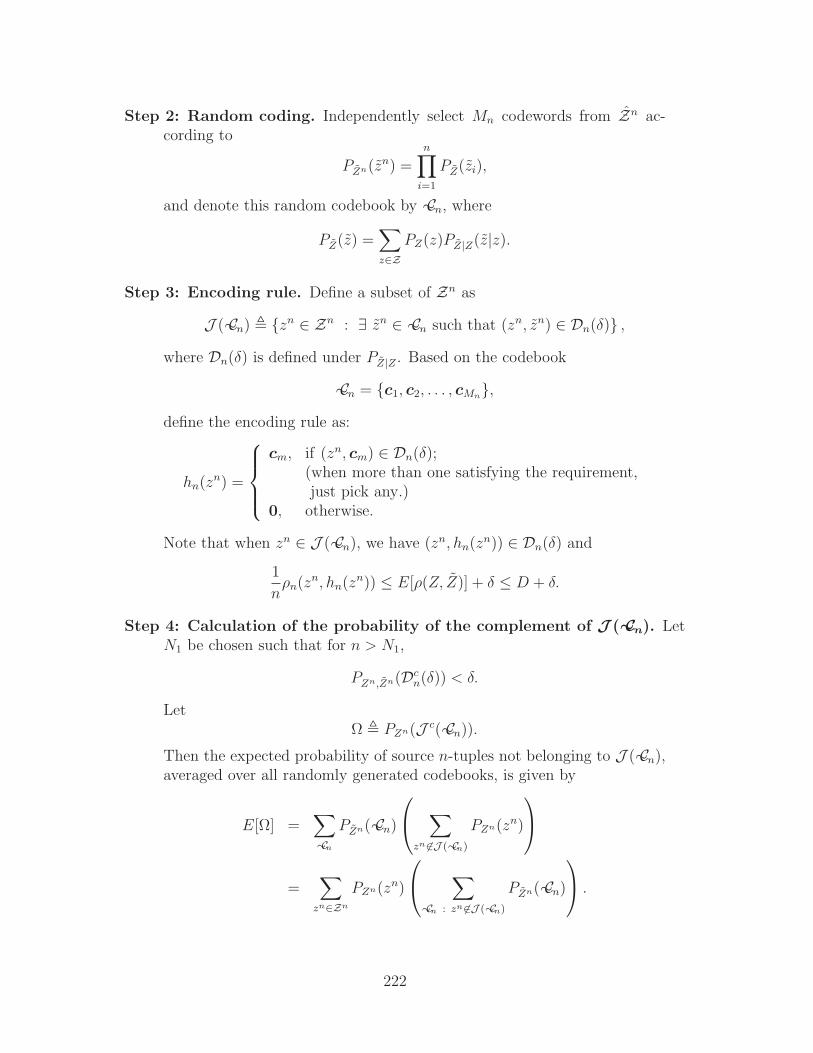
Step 2: Random coding. Independently select Mn codewords from Zn ac-cording to
PZn(zn) =n∏
i=1
PZ(zi),
and denote this random codebook by C∼n, where
PZ(z) =∑
z∈ZPZ(z)PZ|Z(z|z).
Step 3: Encoding rule. Define a subset of Zn as
J ( C∼n) , zn ∈ Zn : ∃ zn ∈ C∼n such that (zn, zn) ∈ Dn(δ) ,
where Dn(δ) is defined under PZ|Z . Based on the codebook
C∼n = c1, c2, . . . , cMn,
define the encoding rule as:
hn(zn) =
cm, if (zn, cm) ∈ Dn(δ);(when more than one satisfying the requirement,just pick any.)
0, otherwise.
Note that when zn ∈ J ( C∼n), we have (zn, hn(zn)) ∈ Dn(δ) and
1
nρn(zn, hn(zn)) ≤ E[ρ(Z, Z)] + δ ≤ D + δ.
Step 4: Calculation of the probability of the complement of J ( C∼n). LetN1 be chosen such that for n > N1,
PZn,Zn(Dcn(δ)) < δ.
LetΩ , PZn(J c( C∼n)).
Then the expected probability of source n-tuples not belonging to J ( C∼n),averaged over all randomly generated codebooks, is given by
E[Ω] =∑
C∼n
PZn( C∼n)
∑
zn 6∈J ( C∼n)
PZn(zn)
=∑
zn∈Zn
PZn(zn)
∑
C∼n : zn 6∈J ( C∼n)
PZn( C∼n)
.
222
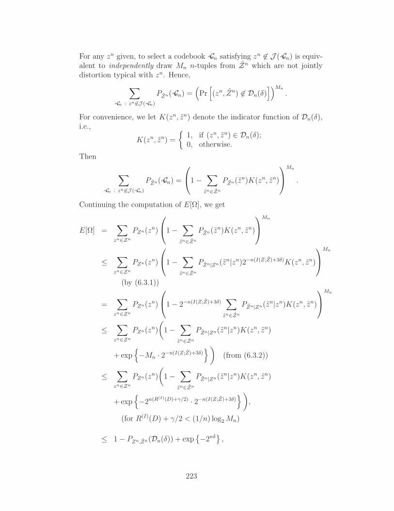
For any zn given, to select a codebook C∼n satisfying zn 6∈ J ( C∼n) is equiv-alent to independently draw Mn n-tuples from Zn which are not jointlydistortion typical with zn. Hence,
∑
C∼n : zn 6∈J ( C∼n)
PZn( C∼n) =(
Pr[
(zn, Zn) 6∈ Dn(δ)])Mn
.
For convenience, we let K(zn, zn) denote the indicator function of Dn(δ),i.e.,
K(zn, zn) =
1, if (zn, zn) ∈ Dn(δ);0, otherwise.
Then
∑
C∼n : zn 6∈J ( C∼n)
PZn( C∼n) =
1 −∑
zn∈Zn
PZn(zn)K(zn, zn)
Mn
.
Continuing the computation of E[Ω], we get
E[Ω] =∑
zn∈Zn
PZn(zn)
1 −∑
zn∈Zn
PZn(zn)K(zn, zn)
Mn
≤∑
zn∈Zn
PZn(zn)
1 −∑
zn∈Zn
PZn|Zn(zn|zn)2−n(I(Z;Z)+3δ)K(zn, zn)
Mn
(by (6.3.1))
=∑
zn∈Zn
PZn(zn)
1 − 2−n(I(Z;Z)+3δ)∑
zn∈Zn
PZn|Zn(zn|zn)K(zn, zn)
Mn
≤∑
zn∈Zn
PZn(zn)
(
1 −∑
zn∈Zn
PZn|Zn(zn|zn)K(zn, zn)
+ exp
−Mn · 2−n(I(Z;Z)+3δ))
(from (6.3.2))
≤∑
zn∈Zn
PZn(zn)
(
1 −∑
zn∈Zn
PZn|Zn(zn|zn)K(zn, zn)
+ exp
−2n(R(I)(D)+γ/2) · 2−n(I(Z;Z)+3δ))
,
(for R(I)(D) + γ/2 < (1/n) log2 Mn)
≤ 1 − PZn,Zn(Dn(δ)) + exp−2nδ
,
223

(for R(I)(D) = I(Z; Z) and δ ≤ γ/8)
= PZn,Zn(Dcn(δ)) + exp
−2nδ
≤ δ + δ = 2δ
for all n > N , max
N0, N1,1δlog2 log
(1
minδ,1
)
.
Since E[Ω] = E [PZn (J c( C∼n))] ≤ 2δ, there must exists a codebook C∼∗n
such that PZn (J c( C∼∗n)) is no greater than 2δ for n sufficiently large.
Step 5: Calculation of distortion. The distortion of the optimal codebookC∼∗
n (from the previous step) satisfies for n > N :
1
nE[ρn(Zn, hn(Zn))] =
∑
zn∈J ( C∼∗n)
PZn(zn)1
nρn(zn, hn(zn))
+∑
zn 6∈J ( C∼∗n)
PZn(zn)1
nρn(zn, hn(zn))
≤∑
zn∈J ( C∼∗n)
PZn(zn)(D + δ) +∑
zn 6∈J ( C∼∗n)
PZn(zn)ρmax
≤ (D + δ) + 2δ · ρmax
≤ D + δ(1 + 2ρmax)
≤ D + ε.
This concludes the proof of the achievability part.
2. Converse Part (i.e., R(D + ε) ≥ R(I)(D) for arbitrarily small ε > 0 andany D ∈ D ≥ 0 : R(I)(D) > 0): We need to show that for any sequence of(n,Mn, Dn)∞n=1 code with
lim supn→∞
1
nlog2 Mn < R(I)(D),
there exists ε > 0 such that
Dn =1
nE[ρn(Zn, hn(Zn))] > D + ε
for n sufficiently large. The proof is as follows.
Step 1: Convexity of mutual information. By the convexity of mutual in-formation I(Z; Z) with respect to PZ|Z for a fixed PZ , we have
I(Z; Zλ) ≤ λ · I(Z; Z1) + (1 − λ) · I(Z; Z2),
224

where λ ∈ [0, 1], and
PZλ|Z(z|z) , λPZ1|Z(z|z) + (1 − λ)PZ2|Z(z|z).
Step 2: Convexity of R(I)(D). Let PZ1|Z and PZ2|Z be two distributions
achieving R(I)(D1) and R(I)(D2), respectively. Since
E[ρ(Z, Zλ)] =∑
z∈ZPZ(z)
∑
z∈Z
PZλ|Z(z|z)ρ(z, z)
=∑
z∈Z,z∈Z
PZ(z)[
λPZ1|Z(z|z) + (1 − λ)PZ2|Z(z|z)]
ρ(z, z)
= λD1 + (1 − λ)D2,
we have
R(I)(λD1 + (1 − λ)D2) ≤ I(Z; Zλ)
≤ λI(Z; Z1) + (1 − λ)I(Z; Z2)
= λR(I)(D1) + (1 − λ)R(I)(D2).
Therefore, R(I)(D) is a convex function.
Step 3: Strictly decreasing and continuity properties of R(I)(D).
By definition, R(I)(D) is non-increasing in D. Also,
R(I)(D) = 0 iff D ≥ Dmax , minz
∑
z∈ZPZ(z)ρ(z, z) (6.3.4)
which is finite by the boundedness of the distortion measure. Thus sinceR(I)(D) is non-increasing and convex, it directly follows that it is strictlydecreasing and continuous over D ≥ 0 : R(I)(D) > 0.
Step 4: Main proof.
log2 Mn ≥ H(hn(Zn))
= H(hn(Zn)) − H(hn(Zn)|Zn), since H(hn(Zn)|Zn) = 0;
= I(Zn; hn(Zn))
= H(Zn) − H(Zn|hn(Zn))
=n∑
i=1
H(Zi) −n∑
i=1
H(Zi|hn(Zn), Z1, . . . , Zi−1)
by the independence of Zn,
and the chain rule for conditional entropy;
225

≥n∑
i=1
H(Zi) −n∑
i=1
H(Zi|Zi)
where Zi is the ith component of hn(Zn);
=n∑
i=1
I(Zi; Zi)
≥n∑
i=1
R(I)(Di), where Di , E[ρ(Zi, Zi)];
= n
n∑
i=1
1
nR(I)(Di)
≥ nR(I)
(n∑
i=1
1
nDi
)
, by convexity of R(I)(D);
= nR(I)
(1
nE[ρn(Zn, hn(Zn))]
)
,
where the last step follows since the distortion measure is additive. Finally,lim supn→∞(1/n) log2 Mn < R(I)(D) implies the existence of N and γ > 0such that (1/n) log Mn < R(I)(D)−γ for all n > N . Therefore, for n > N ,
R(I)
(1
nE[ρn(Zn, hn(Zn))]
)
< R(I)(D) − γ,
which, together with the fact that R(I)(D) is strictly decreasing, impliesthat
1
nE[ρn(Zn, hn(Zn))] > D + ε
for some ε = ε(γ) > 0 and for all n > N .
3. Summary: For D ∈ D ≥ 0 : R(I)(D) > 0, the achievability and converseparts jointly imply that R(I)(D)+4ε ≥ R(D+ε) ≥ R(I)(D) for arbitrarily smallε > 0. These inequalities together with the continuity of R(I)(D) yield thatR(D) = R(I)(D) for D ∈ D ≥ 0 : R(I)(D) > 0.
For D ∈ D ≥ 0 : R(I)(D) = 0, the achievability part gives us R(I)(D)+4ε =4ε ≥ R(D + ε) ≥ 0 for arbitrarily small ε > 0. This immediately implies thatR(D) = 0(= R(I)(D)) as desired. 2
As in the case of block source coding in Chapter 3 (compare Theorem 3.5with Theorem 3.14), the above rate-distortion theorem can be extended for thecase of stationary ergodic sources (e.g., see [97, 27]).
226
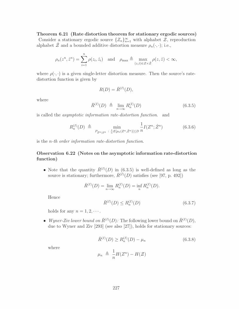
Theorem 6.21 (Rate distortion theorem for stationary ergodic sources)Consider a stationary ergodic source Zn∞n=1 with alphabet Z, reproduction
alphabet Z and a bounded additive distortion measure ρn(·, ·); i.e.,
ρn(zn, zn) =n∑
i=1
ρ(zi, zi) and ρmax , max(z,z)∈Z×Z
ρ(z, z) < ∞,
where ρ(·, ·) is a given single-letter distortion measure. Then the source’s rate-distortion function is given by
R(D) = R(I)(D),
whereR(I)(D) , lim
n→∞R(I)
n (D) (6.3.5)
is called the asymptotic information rate-distortion function. and
R(I)n (D) , min
PZn|Zn : 1n
E[ρn(Zn,Zn)]≤D
1
nI(Zn; Zn) (6.3.6)
is the n-th order information rate-distortion function.
Observation 6.22 (Notes on the asymptotic information rate-distortionfunction)
• Note that the quantity R(I)(D) in (6.3.5) is well-defined as long as thesource is stationary; furthermore, R(I)(D) satisfies (see [97, p. 492])
R(I)(D) = limn→∞
R(I)n (D) = inf
nR(I)
n (D).
HenceR(I)(D) ≤ R(I)
n (D) (6.3.7)
holds for any n = 1, 2, · · · .
• Wyner-Ziv lower bound on R(I)(D): The following lower bound on R(I)(D),due to Wyner and Ziv [293] (see also [27]), holds for stationary sources:
R(I)(D) ≥ R(I)n (D) − µn (6.3.8)
where
µn ,1
nH(Zn) − H(Z)
227

represents the amount of memory in the source and H(Z) = limn→∞1nH(Zn)
is the source entropy rate. Note that as n → ∞, µn → 0; thus the aboveWyner-Ziv lower bound is asymptotically tight in n.1
• When the source Zn is a DMS, it can readily be verified from (6.3.5) and(6.3.6) that
R(I)(D) = R(I)1 (D) = R(I)(D),
where R(I)(D) is given in (6.3.3).
• R(I)(D) for binary symmetric Markov sources: When Zn is a stationarybinary symmetric Markov source, R(I)(D) is partially explicitly known.More specifically, it is shown by Gray [115] that
R(I)(D) = hb(q) − hb(D) for 0 ≤ D ≤ Dc (6.3.9)
where
Dc =1
2
(
1 −√
1 − (1 − q)2
q
)
,
q = PZn = 1|Zn−1 = 0 = PZn = 0|Zn−1 = 1 > 1/2 is the source’stransition probability and hb(p) = −p log2(p) − (1 − p) log2(1 − p) is thebinary entropy function. Determining R(I)(D) for D > Dc is still an openproblem, although R(I)(D) can be estimated in this region via lower andupper bounds. Indeed, the right-sand side of (6.3.9) still serves as a lowerbound on R(I)(D) for D > Dc [115]. Another lower bound on R(I)(D) isthe above Wyner-Ziv bound (6.3.8), while (6.3.7) gives an upper bound.Various bounds on R(I)(D) are studied in [28] and calculated (in particular,see [28, Figure 1]).
The formula of the rate-distortion function obtained in the previous theoremsis also valid for the squared error distortion over the real numbers, even if it isunbounded. Here, we put the boundedness assumption just to facilitate theexposition of the current proof.2 The discussion on lossy data compression,
1A twin result to the above Wyner-Ziv lower bound, which consists of an upper bound on thecapacity-cost function of channels with stationary additive noise, is shown in [11, Corollary 1].This result, which is expressed in terms of the n-th order capacity-cost function and the amountof memory in the channel noise, illustrates the “natural duality” between the information rate-distortion and capacity-cost functions originally pointed out by Shannon [246].
2For example, the boundedness assumption in the theorems can be replaced with assumingthat there exists a reproduction symbol z0 ∈ Z such that E[ρ(Z, z0)] < ∞ [27, Theorem 7.2.4].This assumption can accommodate the squared error distortion measure and a source withfinite second moment (including continuous-alphabet sources such as Gaussian sources); seealso [97, Theorem 9.6.2 and p. 479].
228
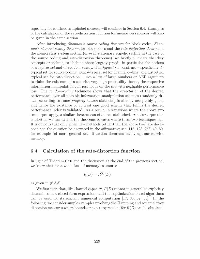
especially for continuous alphabet sources, will continue in Section 6.4. Examplesof the calculation of the rate-distortion function for memoryless sources will alsobe given in the same section.
After introducing Shannon’s source coding theorem for block codes, Shan-non’s channel coding theorem for block codes and the rate-distortion theorem inthe memoryless system setting (or even stationary ergodic setting in the case ofthe source coding and rate-distortion theorems), we briefly elucidate the “keyconcepts or techniques” behind these lengthy proofs, in particular the notionsof a typical-set and of random-coding. The typical-set construct – specifically, δ-typical set for source coding, joint δ-typical set for channel coding, and distortiontypical set for rate-distortion – uses a law of large numbers or AEP argumentto claim the existence of a set with very high probability; hence, the respectiveinformation manipulation can just focus on the set with negligible performanceloss. The random-coding technique shows that the expectation of the desiredperformance over all possible information manipulation schemes (randomly dr-awn according to some properly chosen statistics) is already acceptably good,and hence the existence of at least one good scheme that fulfills the desiredperformance index is validated. As a result, in situations where the above twotechniques apply, a similar theorem can often be established. A natural questionis whether we can extend the theorems to cases where these two techniques fail.It is obvious that only when new methods (other than the above two) are devel-oped can the question be answered in the affirmative; see [116, 128, 258, 49, 50]for examples of more general rate-distortion theorems involving sources withmemory.
6.4 Calculation of the rate-distortion function
In light of Theorem 6.20 and the discussion at the end of the previous section,we know that for a wide class of memoryless sources
R(D) = R(I)(D)
as given in (6.3.3).
We first note that, like channel capacity, R(D) cannot in general be explicitlydetermined in a closed-form expression, and thus optimization based algorithmscan be used for its efficient numerical computation [17, 33, 62, 35]. In thefollowing, we consider simple examples involving the Hamming and squared errordistortion measures where bounds or exact expressions for R(D) can be obtained.
229

6.4.1 Rate-distortion function for discrete memorylesssources under the Hamming distortion measure
A specific application of the rate-distortion function that is useful in practice iswhen the Hamming additive distortion measure is used with a (finite-alphabet)DMS with Z = Z.
We first assume that the DMS is binary-valued (i.e., it is a Bernoulli source)with Z = Z = 0, 1. In this case, the Hamming additive distortion measuresatisfies:
ρn(zn, zn) =n∑
i=1
zi ⊕ zi,
where ⊕ denotes modulo two addition. In such case, ρ(zn, zn) is exactly thenumber of bit errors or changes after compression. Therefore, the distortionbound D becomes a bound on the average probability of bit error. Specifically,among n compressed bits, it is expected to have E[ρ(Zn, Zn)] bit errors; hence,the expected value of bit-error-rate is (1/n)E[ρ(Zn, Zn)]. The rate-distortionfunction for binary sources and Hamming additive distortion measure is givenby the next theorem.
Theorem 6.23 Fix a binary DMS Zn∞n=1 with marginal distribution PZ(0) =1−PZ(1) = p, where 0 < p < 1. Then the source’s rate-distortion function underthe Hamming additive distortion measure is given by:
R(D) =
hb(p) − hb(D) if 0 ≤ D < minp, 1 − p;
0 if D ≥ minp, 1 − p,
where hb(·) is the binary entropy function.
Proof: Assume without loss of generality that p ≤ 1/2.
We first prove the theorem for 0 ≤ D < minp, 1 − p = p. Observe that
H(Z|Z) = H(Z ⊕ Z|Z).
Also observe that
E[ρ(Z, Z)] ≤ D implies that PrZ ⊕ Z = 1 ≤ D.
Then, examining (6.3.3), we have
I(Z; Z) = H(Z) − H(Z|Z)
= hb(p) − H(Z ⊕ Z|Z)
≥ hb(p) − H(Z ⊕ Z) (conditioning never increases entropy)
230
≥ hb(p) − hb(D),
where the last inequality follows since the binary entropy function hb(x) is in-creasing for x ≤ 1/2, and PrZ ⊕ Z = 1 ≤ D. Since the above derivation istrue for any PZ|Z , we have
R(D) ≥ hb(p) − hb(D).
It remains to show that the lower bound is achievable by some PZ|Z , or equiv-
alently, H(Z|Z) = hb(D) for some PZ|Z . By defining PZ|Z(0|0) = PZ|Z(1|1) =
1 − D, we immediately obtain H(Z|Z) = hb(D). The desired PZ|Z can beobtained by simultaneously solving the equations
1 = PZ(0) + PZ(1) =PZ(0)
PZ|Z(0|0)PZ|Z(0|0) +
PZ(0)
PZ|Z(0|1)PZ|Z(1|0)
=p
1 − DPZ|Z(0|0) +
p
D(1 − PZ|Z(0|0))
and
1 = PZ(0) + PZ(1) =PZ(1)
PZ|Z(1|0)PZ|Z(0|1) +
PZ(1)
PZ|Z(1|1)PZ|Z(1|1)
=1 − p
D(1 − PZ|Z(1|1)) +
1 − p
1 − DPZ|Z(1|1),
which yield
PZ|Z(0|0) =1 − D
1 − 2D
(
1 − D
p
)
and
PZ|Z(1|1) =1 − D
1 − 2D
(
1 − D
1 − p
)
.
If 0 ≤ D < minp, 1− p = p, then PZ|Z(0|0) > 0 and PZ|Z(1|1) > 0, completingthe proof.
Finally, the fact that R(D) = 0 for D ≥ minp, 1 − p = p follows directlyfrom (6.3.4) by noting that Dmax = minp, 1 − p = p. 2
The above theorem can be extended for non-binary (finite alphabet) memo-ryless sources resulting in a more complicated (but exact) expression for R(D),see [151]. We instead present a simple lower bound on R(D) for a non-binaryDMS under the Hamming distortion measure; this bound is a special case of theso-called Shannon lower bound on the rate-distortion function of a DMS [246](see also [27], [117], [57, Prob. 10.6]).
231

Theorem 6.24 Fix a DMS Zn∞n=1 with distribution PZ . Then the source’srate-distortion function under the Hamming additive distortion measure andZ = Z satisfies:
R(D) ≥ H(Z) − D log2 (|Z| − 1) − hb(D) for 0 ≤ D ≤ Dmax (6.4.1)
where Dmax is given in (6.3.4) as
Dmax , minz
∑
z∈ZPZ(z)ρ(z, z) = 1 − max
zPZ(z),
H(Z) is the source entropy and hb(·) is the binary entropy function. Further-more, equality holds in the above bound for D ≤ (|Z| − 1) minz∈Z PZ(z).
Proof: The proof is left as an exercise. (Hint: use Fano’s inequality and examinethe equality condition.)
Observation 6.25 (Special cases of Theorem 6.24)
• If the source is binary (i.e., |Z| = 2) with PZ(0) = p, then
(|Z| − 1) minz∈Z
PZ(z) = minp, 1 − p = Dmax.
Thus the condition for equality in (6.4.1) always holds and Theorem 6.24reduces to Theorem 6.23.
• If the source is uniformly distributed (i.e., PZ(z) = 1/|Z| for all z ∈ Z),then
(|Z| − 1) minz∈Z
PZ(z) =|Z| − 1
|Z| = Dmax.
Thus we directly obtain from Theorem 6.24 that
R(D) =
log2(|Z|) − D log2 (|Z| − 1) − hb(D), if 0 ≤ D ≤ |Z|−1|Z| ;
0, if D > |Z|−1|Z| .
(6.4.2)
6.4.2 Rate-distortion function for continuous memorylesssources under the squared error distortion measure
We next examine the calculation or bounding of the rate-distortion functionfor continuous memoryless sources under the additive squared error distortionmeasure. We first show that the Gaussian source maximizes the rate-distortion
232

function among all continuous sources with identical variance. This result, whoseproof uses the fact that the Gaussian distribution maximizes differential entropyamong all real-valued sources with the same variance (Theorem 5.20), can beseen as a dual result to Theorem 5.33, which states that Gaussian noise minimizesthe capacity of additive-noise channels. We also obtain the Shannon lower boundon the rate-distortion function of continuous sources under the squared errordistortion measure.
Theorem 6.26 (Gaussian sources maximize the rate-distortion func-tion) Under the additive squared error distortion measure, namely ρn(zn, zn) =∑n
i=1(zi− zi)2, the rate-distortion function for any continuous memoryless source
Zi with a pdf of support R, zero mean, variance σ2 and finite differential en-tropy satisfies
R(D) ≤
1
2log2
σ2
D, for 0 < D ≤ σ2
0, for D > σ2
with equality holding when the source is Gaussian.
Proof: By Theorem 6.20 (extended to the “unbounded” squared error distortionmeasure),
R(D) = R(I)(D) = minfZ|Z : E[(Z−Z)2]≤D
I(Z; Z).
So for any fZ|Z satisfying the distortion constraint,
R(D) ≤ I(fZ , fZ|Z).
For 0 < D ≤ σ2, choose a dummy Gaussian random variable W with zeromean and variance aD, where a = 1 − D/σ2, and is independent of Z. LetZ = aZ + W . Then
E[(Z − Z)2] = E[(1 − a)2Z2] + E[W 2] = (1 − a)2σ2 + aD = D
which satisfies the distortion constraint. Note that the variance of Z is equal toE[a2Z2] + E[W 2] = σ2 − D. Consequently,
R(D) ≤ I(Z; Z)
= h(Z) − h(Z|Z)
= h(Z) − h(W + aZ|Z)
= h(Z) − h(W |Z) (by Lemma 5.14)
= h(Z) − h(W ) (by the independence of W and Z)
= h(Z) − 1
2log2(2πe(aD))
233
≤ 1
2log2(2πe(σ2 − D)) − 1
2log2(2πe(aD)) (by Theorem 5.20)
=1
2log2
σ2
D.
For D > σ2, let Z satisfy PrZ = 0 = 1 and be independent of Z. ThenE[(Z − Z)2] = E[Z2] + E[Z2] − 2E[Z]E[Z] = σ2 < D, and I(Z; Z) = 0. Hence,R(D) = 0 for D > σ2.
The achievability of this upper bound by a Gaussian source (with zero meanand variance σ2) can be proved by showing that under the Gaussian source,(1/2) log2(σ
2/D) is a lower bound to R(D) for 0 < D ≤ σ2. Indeed, when thesource is Gaussian and for any fZ|Z such that E[(Z − Z)2] ≤ D, we have
I(Z; Z) = h(Z) − h(Z|Z)
=1
2log2(2πeσ2) − h(Z − Z|Z)
≥ 1
2log2(2πeσ2) − h(Z − Z) (by Lemma 5.14)
≥ 1
2log2(2πeσ2) − 1
2log2
(
2πe Var[(Z − Z)])
(byTheorem 5.20)
≥ 1
2log2(2πeσ2) − 1
2log2
(
2πe E[(Z − Z)2])
≥ 1
2log2(2πeσ2) − 1
2log2 (2πeD)
=1
2log2
σ2
D.
2
Theorem 6.27 (Shannon lower bound on the rate-distortion function:squared error distortion) Consider a continuous memoryless source Zi witha pdf of support R and finite differential entropy under the additive squared errordistortion measure. Then its rate-distortion function satisfies
R(D) ≥ h(Z) − 1
2log2(2πeD).
Proof: The proof, which follows similar steps as in the achievability of the upperbound in the proof of the previous theorem, is left as an exercise. 2
The above two theorems yield that for any continuous memoryless sourceZi with zero mean and variance σ2, its rate-distortion function under themean-square error distortion measure satisfies
RSH(D) ≤ R(D) ≤ RG(D) for 0 < D ≤ σ2 (6.4.3)
234

where
RSH(D) , h(Z) − 1
2log2(2πeD)
and
RG(D) ,1
2log2
σ2
D
and with equality holding when the source is Gaussian. Thus, the differencebetween the upper and lower bounds on R(D) in (6.4.3) is
RG(D) − RSH(D) = −h(Z) +1
2log2(2πeσ2)
= D(Z‖ZG) (6.4.4)
where D(Z‖ZG) is the non-Gaussianness of Z, i.e., the divergence between Zand a Gaussian random variable ZG of mean zero and variance σ2.
Thus the gap between the upper and lower bounds in (6.4.4) is zero if thesource is Gaussian and strictly positive if the source is non-Gaussian. For exam-ple, if Z is uniformly distributed on the interval [−
√3σ2,
√3σ2] and hence with
variance σ2, then D(Z‖ZG) = 0.255 bits for σ2 = 1. On the other hand, if Z isLaplacian distributed with variance σ2 or parameter σ/
√2(its pdf is given by
fZ(z) = 1√2σ2
exp −√
2|z|σ
for z ∈ R), then D(Z‖ZG) = 0.104 bits for σ2 = 1.
We can thus deduce that the Laplacian source is more similar to the Gaus-sian source than the uniformly distributed source and hence its rate-distortionfunction is closer to Gaussian’s rate-distortion function RG(D) than that of auniform source. Finally in light of (6.4.4), the bounds on R(D) in (6.4.3) canbe expressed in terms of the Gaussian rate-distortion function RG(D) and thenon-Gaussianness D(Z‖ZG), as follows
RG(D) − D(Z‖ZG) ≤ R(D) ≤ RG(D) for 0 < D ≤ σ2. (6.4.5)
Note that (6.4.5) is nothing but the dual of (5.7.4) and is an illustration of theduality between the rate-distortion and capacity-cost functions.
6.4.3 Rate-distortion function for continuous memorylesssources under the absolute error distortion measure
We herein focus on the rate-distortion function of continuous memoryless sourcesunder the absolute error distortion measure. In particular, we show that amongall zero-mean real-valued sources with absolute mean λ (i.e., E[|Z|] = λ), theLaplacian source with parameter λ (i.e., with variance 2λ2) maximizes the rate-distortion function. This result, which also provides the expression of the rate-distortion function of Laplacian sources, is similar to Theorem 6.26 regarding
235
the maximal rate-distortion function under the squared error distortion measure(which is achieved by Gaussian sources). It is worth pointing out that in imagecoding applications, the Laplacian distribution is a good model to approximatethe statistics of transform coefficients such as discrete cosine and wavelet trans-form coefficients [226, 267]. Finally, analogously to Theorem 6.27, we obtain aShannon lower bound on the rate-distortion function under the absolute errordistortion.
Theorem 6.28 (Laplacian sources maximize the rate-distortion func-tion) Under the additive absolute error distortion measure, namely ρn(zn, zn) =∑n
i=1 |zi − zi|, the rate-distortion function for any continuous memoryless sourceZi with a pdf of support R, zero mean and E|Z| = λ, where λ > 0 is a fixedparameter, satisfies
R(D) ≤
log2
λ
D, for 0 < D ≤ λ
0, for D > λ
with equality holding when the source is Laplacian with mean zero and variance
2λ2 (parameter λ); i.e., its pdf is given by fZ(z) = 12λ
e−|z|λ , z ∈ R.
Proof: SinceR(D) = min
fZ|Z : E[|Z−Z|]≤DI(Z; Z),
we have that for any fZ|Z satisfying the distortion constraint,
R(D) ≤ I(Z; Z) = I(fZ , fZ|Z).
For 0 < D ≤ λ, choose
Z =
(
1 − D
λ
)2
Z + sgn(Z)|W |,
where sgn(Z) is equal to 1 if Z ≥ 0 and to −1 if Z < 0, and W is a dummyrandom variable that is independent of Z and has a Laplacian distribution withmean zero and E[|W |] = (1 − D/λ)D; i.e., with parameter (1 − D/λ)D. Thus
E[|Z|] = E
∣∣∣∣∣
(
1 − D
λ
)2
Z + sgn(Z)|W |∣∣∣∣∣
=
(
1 − D
λ
)2
E[|Z|] + E[|W |]
236
=
(
1 − D
λ
)2
λ +
(
1 − D
λ
)
D
= λ − D (6.4.6)
and
E[|Z − Z|] = E
∣∣∣∣∣
(
1 − D
λ
)2
Z + sgn(Z)|W | − Z
∣∣∣∣∣
= E
∣∣∣∣
D
λ
(
2 − D
λ
)
Z − sgn(Z)W
∣∣∣∣
=D
λ
(
2 − D
λ
)
E[|Z|] − E[|W |]
=D
λ
(
2 − D
λ
)
λ −(
1 − D
λ
)
D
= D,
and hence this choice of Z satisfies the distortion constraint. We can thereforewrite for this Z that
R(D) ≤ I(Z; Z)
= h(Z) − h(Z|Z)(a)= h(Z) − h(sgn(Z)|W | |Z)
= h(Z) − h(|W | |Z) − log2 |sgn(Z)|(b)= h(Z) − h(|W |)(c)= h(Z) − h(W )(d)= h(Z) − log2[2e(1 − D/λ)D](e)
≤ log2[2e(λ − D)] − log2[2e(1 − D/λ)D]
= log2
λ
D,
where (a) follows from the expression of Z and the fact that differential entropyis invariant under translations (Lemma 5.14), (b) holds since Z and W areindependent of each other, (c) follows from the fact that W is Laplacian andthat the Laplacian is symmetric, and (d) holds since the differential entropy ofa zero-mean Laplacian random variable Z ′ with E[|Z ′|] = λ′ is given by
h(Z ′) = log2(2eλ′) (in bits).
Finally, (e) follows by noting that E[|Z|] = λ − D from (6.4.6) and from thefact among all zero-mean real-valued random variables Z ′ with E[|Z ′|] = λ′, the
237
Laplacian random variable with zero-mean and parameter λ′ maximizes differ-ential entropy (see Observation 5.21, item 3).
For D > λ, let Z satisfy Pr(Z = 0) = 1 and be independent of Z. ThenE[|Z − Z| ≤ E[|Z|]+E[|Z|] = λ < D. For this choice of Z, R(D) ≤ I(Z; Z) = 0and hence R(D) = 0. This completes the proof of the upper bound.
We next show that the upper bound can be achieved by a Laplacian sourcewith mean zero and parameter λ. This is proved by showing that for a Laplaciansource with mean zero and parameter λ, (1/2) log2(λ/D) is a lower bound toR(D) for 0 < D ≤ λ: for such a Laplacian source and for any fZ|Z satisfying
E[|Z − Z|] ≤ D, we have
I(Z; Z) = h(Z) − h(Z|Z)
= log2(2eλ) − h(Z − Z|Z)
≥ log2(2eλ) − h(Z − Z) (by Lemma 5.14)
≥ log2(2eλ) − log2(2eD)
= log2
λ
D,
where the last inequality follows since
h(Z − Z) ≤ log2
(
2eE[|Z − Z|])
≤ log2(2eD)
by Observation 5.21 and the fact that E[|Z − Z|] ≤ D. 2
Theorem 6.29 (Shannon lower bound on the rate-distortion function:absolute error distortion) Consider a continuous memoryless source Ziwith a pdf of support R and finite differential entropy under the additive absoluteerror distortion measure. Then its rate-distortion function satisfies
R(D) ≥ h(Z) − log2(2eD).
Proof: The proof is left as an exercise. 2
Observation 6.30 (Shannon lower bound on the rate-distortion func-tion: difference distortion) The general form of the Shannon lower boundfor a source Zi with finite differential entropy under the difference distortionmeasure ρ(z, z) = d(x− x), where d(·, ·) is a non-negative function, is as follows
R(D) ≥ h(Z) − supX:E[d(X)]≤D
h(X)
where the supremum is taken over all random variables X with a pdf satisfyingE[d(X)] ≤ D. It can be readily seen that this bound encompasses those inTheorems 6.27 and 6.29 as special cases.3
3The asymptotic tightness of this bound as D approaches zero is studied in [180].
238
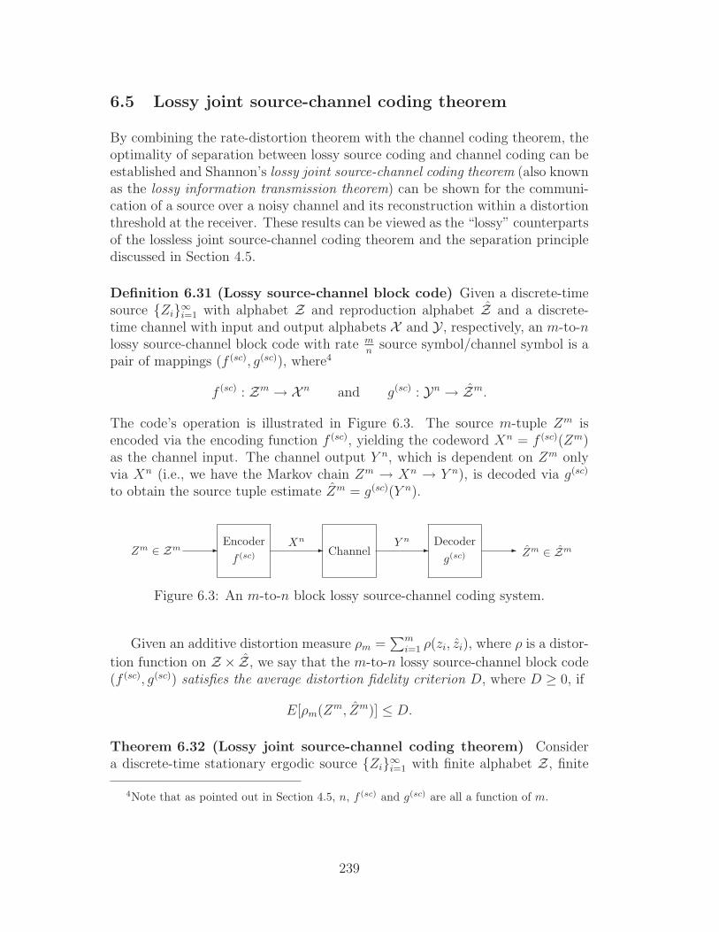
6.5 Lossy joint source-channel coding theorem
By combining the rate-distortion theorem with the channel coding theorem, theoptimality of separation between lossy source coding and channel coding can beestablished and Shannon’s lossy joint source-channel coding theorem (also knownas the lossy information transmission theorem) can be shown for the communi-cation of a source over a noisy channel and its reconstruction within a distortionthreshold at the receiver. These results can be viewed as the “lossy” counterpartsof the lossless joint source-channel coding theorem and the separation principlediscussed in Section 4.5.
Definition 6.31 (Lossy source-channel block code) Given a discrete-timesource Zi∞i=1 with alphabet Z and reproduction alphabet Z and a discrete-time channel with input and output alphabets X and Y , respectively, an m-to-nlossy source-channel block code with rate m
nsource symbol/channel symbol is a
pair of mappings (f (sc), g(sc)), where4
f (sc) : Zm → X n and g(sc) : Yn → Zm.
The code’s operation is illustrated in Figure 6.3. The source m-tuple Zm isencoded via the encoding function f (sc), yielding the codeword Xn = f (sc)(Zm)as the channel input. The channel output Y n, which is dependent on Zm onlyvia Xn (i.e., we have the Markov chain Zm → Xn → Y n), is decoded via g(sc)
to obtain the source tuple estimate Zm = g(sc)(Y n).
Zm ∈ Zm - Encoder
f (sc)-Xn
Channel -Y n Decoder
g(sc)- Zm ∈ Zm
Figure 6.3: An m-to-n block lossy source-channel coding system.
Given an additive distortion measure ρm =∑m
i=1 ρ(zi, zi), where ρ is a distor-
tion function on Z × Z, we say that the m-to-n lossy source-channel block code(f (sc), g(sc)) satisfies the average distortion fidelity criterion D, where D ≥ 0, if
E[ρm(Zm, Zm)] ≤ D.
Theorem 6.32 (Lossy joint source-channel coding theorem) Considera discrete-time stationary ergodic source Zi∞i=1 with finite alphabet Z, finite
4Note that as pointed out in Section 4.5, n, f (sc) and g(sc) are all a function of m.
239

reproduction alphabet Z, bounded additive distortion measure ρm(·, ·) and rate-distortion function R(D),5 and consider a discrete-time memoryless channel withinput alphabet X , output alphabet Y and capacity C.6 Assuming that bothR(D) and C are measured in the same units, the following hold:
• Forward part (achievability): For any D > 0, there exists a sequence ofm-to-nm lossy source-channel codes (f (sc), g(sc)) satisfying the average dis-tortion fidelity criterion D for sufficiently large m if
(
lim supm→∞
m
nm
)
· R(D) < C.
• Converse part: On the other hand, for any sequence of m-to-nm lossysource-channel codes (f (sc), g(sc)) satisfying the average distortion fidelitycriterion D, we have (
m
nm
)
· R(D) ≤ C.
Proof: The proof uses both the channel coding theorem (i.e., Theorem 4.10)and the rate-distortion theorem (i.e., Theorem 6.21) and follows similar argu-ments as the proof of the lossless joint source-channel coding theorem presentedin Section 4.5. We leave the proof as an exercise.
Observation 6.33 (Lossy joint source-channel coding theorem with sig-naling rates) The above theorem also admits another form when the sourceand channel are described in terms of “signaling rates” (e.g., [35]). More specif-ically, let Ts and Tc represent the durations (in seconds) per source letter andper channel input symbol, respectively.7 In this case, Tc
Tsrepresents the source-
channel transmission rate measured in source symbols per channel use (or inputsymbol). Thus, again assuming that both R(D) and C are measured in the sameunits, the theorem becomes as follows:
• The source can be reproduced at the output of the channel with distortionless than D (i.e., there exist lossy source-channel codes asymptotically
5Note that Z and Z can also be continuous alphabets with an unbounded distortion func-tion. In this case, the theorem still holds under appropriate conditions (e.g., [27, Problem 7.5],[97, Theorem 9.6.3]) that can accommodate for example the important class of Gaussiansources under the squared error distortion function (e.g., [97, p. 479]).
6The channel can have either finite or continuous alphabets. For example, it can be thememoryless Gaussian (i.e., AWGN) channel with input power P ; in this case, C = C(P ).
7In other words, the source emits symbols at a rate of 1/Ts source symbols per second andthe channel accepts inputs at a rate of 1/Tc channel symbols per second.
240

satisfying the average distortion fidelity criterion D) if
(Tc
Ts
)
· R(D) < C.
• Conversely, for any lossy source-channel codes satisfying the average dis-tortion fidelity criterion D, we have
(Tc
Ts
)
· R(D) ≤ C.
6.6 Shannon limit of communication systems
We close this chapter by applying Theorem 6.32 to a few useful examples ofcommunication systems. Specifically, we obtain a bound on the end-to-end dis-tortion of any communication system by using the fact that if a source withrate-distortion function R(D) can be transmitted over a channel with capacityC via a source-channel block code of rate Rsc > 0 (in source symbols/channeluse) and reproduced at the destination with an average distortion no larger thanD, then we must have that
Rsc · R(D) ≤ C
or equivalently,
R(D) ≤ 1
Rsc
C. (6.6.1)
Solving for the smallest D, say DSL, satisfying (6.6.1) with equality8 yields alower bound, called the Shannon limit,9 on the distortion of all realizable lossysource-channel codes for the system with rate Rsc.
In the following examples, we calculate the Shannon limit for some source-channel configurations. The Shannon limit is not necessarily achievable in gen-eral, although this is the case in the first two examples.
Example 6.34 (Shannon limit for a binary uniform DMS over a BSC)10
Let Z = Z = 0, 1 and consider a binary uniformly distributed DMS Zi (i.e.,a Bernoulli(1/2) source) using the additive Hamming distortion measure. Note
8If the strict inequality R(D) < 1Rsc
C always holds, then in this case, the Shannon limit
is DSL = Dmin , E[minz∈Z ρ(Z, z)
].
9Other similar quantities used in the literature are the optimal performance theoreticallyachievable (OPTA) [27] and the limit of the minimum transmission ratio (LMTR) [61].
10This example appears in various sources including [149, Section 11.8], [61, Problem 2.2.16]and [188, Problem 5.7].
241
that in this case, E[ρ(Z, Z)] = P (Z 6= Z) , Pb ; in other words, the expecteddistortion is nothing but the source’s bit error probability Pb. We desire totransmit the source over a BSC with crossover probability ǫ < 1/2.
From Theorem 6.23, we know that for 0 ≤ D ≤ 1/2, the source’s rate-distortion function is given by
R(D) = 1 − hb(D),
where hb(·) is the binary entropy function. Also from (4.4.5), the channel’scapacity is given by
C = 1 − hb(ǫ).
The Shannon limit DSL for this system with source-channel transmission rateRsc is determined by solving (6.6.1) with equality:
1 − hb(DSL) =1
Rsc
[1 − hb(ǫ)].
This yields that
DSL = h−1b
(
1 − 1 − hb(ǫ)
Rsc
)
(6.6.2)
for DSL ≤ 1/2, where for any t ≥ 0,
h−1b (t) ,
infx : t = hb(x), if 0 ≤ t ≤ 1
0, if t > 1(6.6.3)
is the inverse of the binary entropy function on the interval [0, 1/2]. Thus DSL
given in (6.6.2) gives a lower bound on the bit error probability Pb of any rate-Rsc source-channel code used for this system. In particular, if Rsc = 1 sourcesymbol/channel use, we directly obtain from (6.6.2) that11
DSL = ǫ. (6.6.4)
Shannon limit over an equivalent binary-input hard-decision demodulated AWGNchannel: It is well-known that a BSC with crossover probability ǫ represents abinary-input AWGN channel used with antipodal (BPSK) signaling and hard-decision coherent demodulation (e.g., see [179]). More specifically, if the channelhas noise power σ2
N = N0/2 (i.e., the channel’s underlying continuous-time white
11Source-channel systems with rate Rsc = 1 are typically referred to as systems with matchedsource and channel bandwidths (or signaling rates). Also, when Rsc < 1 (resp., > 1), thesystem is said to have bandwidth compression (resp., bandwidth expansion); e.g., cf. [193, 225,256].
242
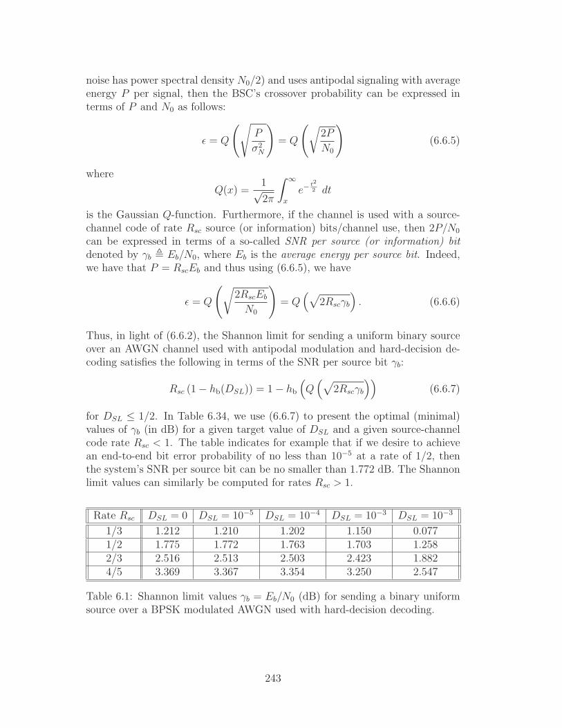
noise has power spectral density N0/2) and uses antipodal signaling with averageenergy P per signal, then the BSC’s crossover probability can be expressed interms of P and N0 as follows:
ǫ = Q
(√
P
σ2N
)
= Q
(√
2P
N0
)
(6.6.5)
where
Q(x) =1√2π
∫ ∞
x
e−t2
2 dt
is the Gaussian Q-function. Furthermore, if the channel is used with a source-channel code of rate Rsc source (or information) bits/channel use, then 2P/N0
can be expressed in terms of a so-called SNR per source (or information) bitdenoted by γb , Eb/N0, where Eb is the average energy per source bit. Indeed,we have that P = RscEb and thus using (6.6.5), we have
ǫ = Q
(√
2RscEb
N0
)
= Q(√
2Rscγb
)
. (6.6.6)
Thus, in light of (6.6.2), the Shannon limit for sending a uniform binary sourceover an AWGN channel used with antipodal modulation and hard-decision de-coding satisfies the following in terms of the SNR per source bit γb:
Rsc (1 − hb(DSL)) = 1 − hb
(
Q(√
2Rscγb
))
(6.6.7)
for DSL ≤ 1/2. In Table 6.34, we use (6.6.7) to present the optimal (minimal)values of γb (in dB) for a given target value of DSL and a given source-channelcode rate Rsc < 1. The table indicates for example that if we desire to achievean end-to-end bit error probability of no less than 10−5 at a rate of 1/2, thenthe system’s SNR per source bit can be no smaller than 1.772 dB. The Shannonlimit values can similarly be computed for rates Rsc > 1.
Rate Rsc DSL = 0 DSL = 10−5 DSL = 10−4 DSL = 10−3 DSL = 10−3
1/3 1.212 1.210 1.202 1.150 0.0771/2 1.775 1.772 1.763 1.703 1.2582/3 2.516 2.513 2.503 2.423 1.8824/5 3.369 3.367 3.354 3.250 2.547
Table 6.1: Shannon limit values γb = Eb/N0 (dB) for sending a binary uniformsource over a BPSK modulated AWGN used with hard-decision decoding.
243

Optimality of uncoded communication: Note that for Rsc = 1, the Shannonlimit in (6.6.4) can surprisingly be achieved by a simple uncoded scheme:12 justdirectly transmit the source over the channel (i.e., set the blocklength m = 1and the channel input Xi = Zi for any time instant i = 1, 2, · · · ) and declare thechannel output as the reproduced source symbol (i.e., set Zi = Yi for any i).13
In this case, the expected distortion (i.e., bit error probability) of this un-coded rate-one source-channel scheme is indeed given as follows:
E[ρ(Z, Z)] = Pb
= P (X 6= Y )
= P (Y 6= X|X = 1)(1/2) + P (Y 6= X|X = 0)(1/2)
= ǫ
= DSL.
We conclude that this rate-one uncoded source-channel scheme achieves theShannon limit and is hence optimal. Furthermore, this scheme, which has noencoding/decoding delay and no complexity), is clearly more desirable than us-ing a separate source-channel coding scheme,14 which would impose large encod-ing and decoding delays and would demand significant computational/storageresources.
Note that for rates Rsc 6= 1 and/or non-uniform sources, the uncoded schemeis not optimal and hence more complicated joint or separate source-channel codeswould be required to yield a bit error probability arbitrarily close to (but strictlylarger than) the Shannon limit DSL. Finally, we refer the reader to [102], wherenecessary and sufficient conditions are established for source-channel pairs underwhich uncoded schemes are optimal.
Observation 6.35 The following two systems are extensions of the system con-sidered in the above example.
• Binary non-uniform DMS over a BSC: The system is identical tothat of Example 6.34 with the exception that the binary DMS is non-uniformly distributed with P (Z = 0) = p. Using the expression of R(D)from Theorem 6.23, it can be readily shown that this system’s Shannon
12Uncoded transmission schemes are also referred to as scalar or single-letter codes.
13In other words, the code’s encoding and decoding functions, f (sc) and g(sc), respectively,are both equal to the identity mapping.
14Note that in this system, since the source is incompressible, no source coding is actuallyrequired. Still the separate coding scheme will consist of a near-capacity achieving channelcode.
244

limit is given by
DSL = h−1b
(
hb(p) − 1 − hb(ǫ)
Rsc
)
(6.6.8)
for DSL ≤ minp, 1− p, where h−1b (·) is the inverse of the binary entropy
function on the interval [0, 1/2] defined in (6.6.3). Setting p = 1/2 in(6.6.8) directly results in the Shannon limit given in (6.6.2), as expected.
• Non-binary uniform DMS over a non-binary symmetric channel:Given integer q ≥ 2, consider a q-ary uniformly distributed DMS withidentical alphabet and reproduction alphabet Z = Z = 0, 1, · · · , q − 1using the additive Hamming distortion measure and the q-ary symmetricDMC (with q-ary input and output alphabets and symbol error rate ǫ)described in (4.2.11). Thus using the expressions for the source’s rate-distortion function in (6.4.2) and the channel’s capacity in Example 4.16,we obtain that the Shannon limit of the system using rate-Rsc source-channel codes satisfies
log2(q)−DSL log2(q − 1)− hb(DSL) =1
Rsc
[log2(q) − ǫ log2(q − 1) − hb(ǫ)]
(6.6.9)for DSL ≤ q−1
q. Setting q = 2 renders the source a Bernoulli(1/2) source
and the channel a BSC with crossover probability ǫ, thus reducing (6.6.9)to (6.6.2).
Example 6.36 (Shannon limit for a memoryless Gaussian source overan AWGN channel [108]) Let Z = Z = R and consider a memoryless Gaus-sian source Zi of mean zero and variance σ2 and the squared error distortionfunction. The objective is to transmit the source over an AWGN channel withinput power constraint P and noise variance σ2
N and recover it with distortionfidelity no larger than D, for a given threshold D > 0.
By Theorem 6.26, the source’s rate-distortion function is given by
R(D) =1
2log2
σ2
Dfor 0 < D < σ2.
Furthermore, the capacity (or capacity-cost function) of the AWGN channel isgiven in (5.4.13) as
C(P ) =1
2log2
(
1 +P
σ2N
)
.
The Shannon limit DSL for this system with rate Rsc is obtained by solving
R(DSL) =C(P )
Rsc
245

or equivalently,1
2log2
σ2
DSL
=1
2Rsc
log2
(
1 +P
σ2N
)
for 0 < DSL < σ2, which gives
DSL =σ2
(
1 + Pσ2
N
) 1Rsc
. (6.6.10)
In particular, for a system with rate Rsc = 1, the Shannon limit in (6.6.10)becomes
DSL =σ2σ2
N
P + σ2N
. (6.6.11)
Optimality of a simple rate-one scalar source-channel coding scheme: The fol-lowing simple (uncoded) source-channel coding scheme with rate Rsc = 1 canachieve the Shannon limit in (6.6.11). The code’s encoding and decoding func-tions are scalar (with m=1). More specifically, at any time instant i, the channelinput (with power constraint P ) is given by
Xi = f (sc)(Zi) =
√
P
σ2Zi,
and is sent over the AWGN channel. At the receiver, the corresponding channeloutput Yi = Xi + Ni, where Ni is the additive Gaussian noise (which is inde-pendent of Zi), is decoded via a scalar (MMSE) detector to yield the followingreconstructed source symbol Zi
Zi = g(sc)(Yi) =
√Pσ2
P + σ2N
Yi.
A simple calculation reveals that this code’s expected distortion is given by
E[(Z − Z)2] = E
(
Z −√
Pσ2
P + σ2N
(√
P
σ2Z + N
))2
=σ2σ2
N
P + σ2N
= DSL,
which proves the optimality of this simple (delayless) source-channel code.
Extensions on the optimality of similar uncoded (scalar) schemes in Gaussiansensor networks can be found in [103, 25].
246

Example 6.37 (Shannon limit for a memoryless Gaussian source overa fading channel) Consider the same system as the above example except thatnow the channel is a memoryless fading channel as described in Observation 5.35with input power constraint P and noise variance σ2
N . We determine the Shannonlimit of this system with rate Rsc for two cases: (1) the fading coefficients areknown at the receiver, and (2) the fading coefficients are known at both thereceiver and the transmitter.
1. Shannon limit with decoder side information (DSI): Using (5.4.17) for thechannel capacity with DSI, we obtain that the Shannon limit with DSI isgiven by
D(DSI)SL =
σ2
2
8<:EA
24log2
„1+ A2P
σ2N
« 1Rsc
35
9=;
(6.6.12)
for 0 < D(DSI)SL < σ2. Making the fading process deterministic by setting
A = 1 (almost surely) reduces (6.6.12) to (6.6.10), as expected.
2. Shannon limit with full side information (FSI): Similarly, using (5.4.19)for the fading channel capacity with FSI, we obtain the following Shannonlimit:
D(FSI)SL =
σ2
2
8<:EA
24log2
„1+
A2p∗(A)
σ2N
« 1Rsc
35
9=;
(6.6.13)
for 0 < D(FSI)SL < σ2, where p∗(·) in (6.6.13) is given by
p∗(a) = max
(
0,1
λ− σ2
a2
)
and λ is chosen to satisfy EA[p(A)] = P .
Example 6.38 (Shannon limit for a binary uniform DMS over a binary-input AWGN channel) Consider the same binary uniform source as in Exam-ple 6.34 under the Hamming distortion measure to be sent via a source-channelcode over a binary-input AWGN channel used with antipodal (BPSK) signalingof power P and noise variance σ2
N = N0/2. Again, here the expected distortionis nothing but the source’s bit error probability Pb. The source’s rate-distortionfunction is given by Theorem 6.23 as presented in Example 6.34.
However, the channel capacity C(P ) of the AWGN whose input takes on twopossible values +
√P or −
√P , whose output is real-valued (unquantized) and
247
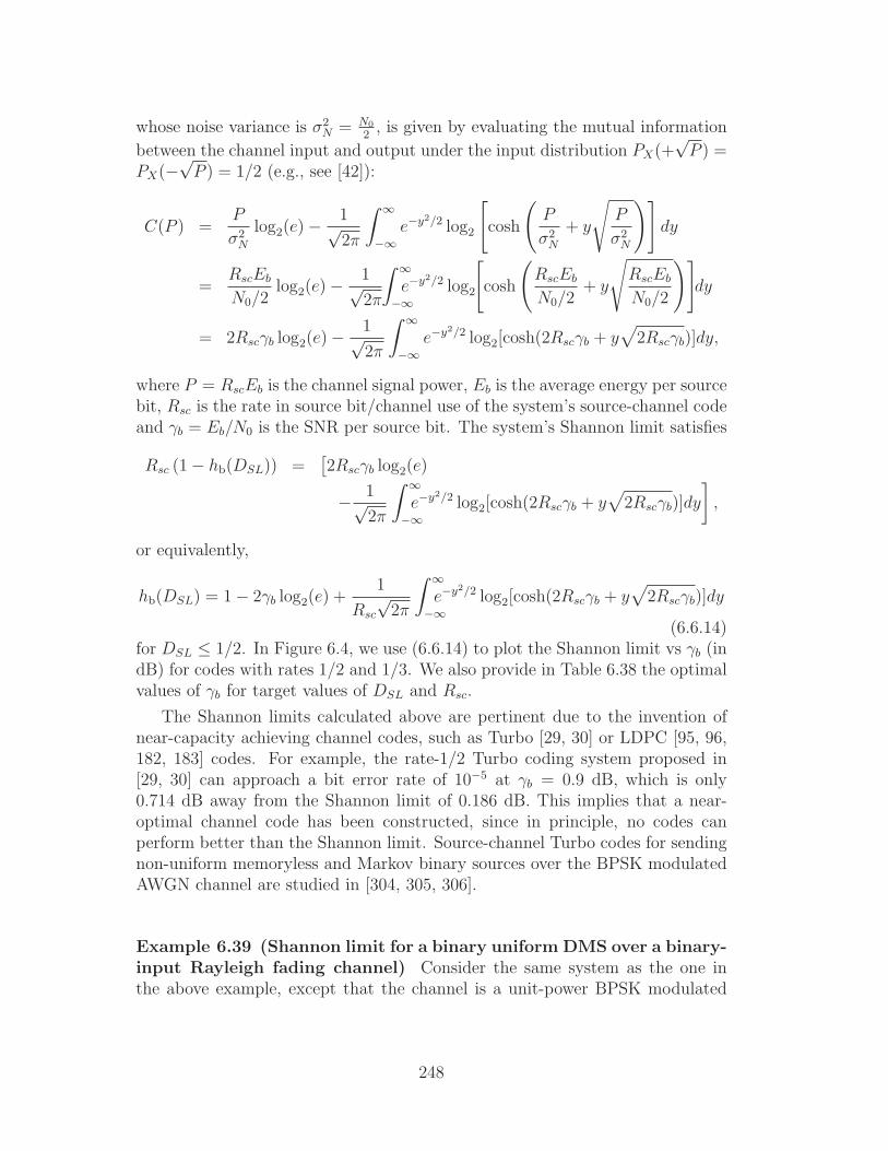
whose noise variance is σ2N = N0
2, is given by evaluating the mutual information
between the channel input and output under the input distribution PX(+√
P ) =PX(−
√P ) = 1/2 (e.g., see [42]):
C(P ) =P
σ2N
log2(e) −1√2π
∫ ∞
−∞e−y2/2 log2
[
cosh
(
P
σ2N
+ y
√
P
σ2N
)]
dy
=RscEb
N0/2log2(e) −
1√2π
∫ ∞
−∞e−y2/2 log2
[
cosh
(
RscEb
N0/2+ y
√
RscEb
N0/2
)]
dy
= 2Rscγb log2(e) −1√2π
∫ ∞
−∞e−y2/2 log2[cosh(2Rscγb + y
√
2Rscγb)]dy,
where P = RscEb is the channel signal power, Eb is the average energy per sourcebit, Rsc is the rate in source bit/channel use of the system’s source-channel codeand γb = Eb/N0 is the SNR per source bit. The system’s Shannon limit satisfies
Rsc (1 − hb(DSL)) =[2Rscγb log2(e)
− 1√2π
∫ ∞
−∞e−y2/2 log2[cosh(2Rscγb + y
√
2Rscγb)]dy
]
,
or equivalently,
hb(DSL) = 1 − 2γb log2(e) +1
Rsc
√2π
∫ ∞
−∞e−y2/2 log2[cosh(2Rscγb + y
√
2Rscγb)]dy
(6.6.14)for DSL ≤ 1/2. In Figure 6.4, we use (6.6.14) to plot the Shannon limit vs γb (indB) for codes with rates 1/2 and 1/3. We also provide in Table 6.38 the optimalvalues of γb for target values of DSL and Rsc.
The Shannon limits calculated above are pertinent due to the invention ofnear-capacity achieving channel codes, such as Turbo [29, 30] or LDPC [95, 96,182, 183] codes. For example, the rate-1/2 Turbo coding system proposed in[29, 30] can approach a bit error rate of 10−5 at γb = 0.9 dB, which is only0.714 dB away from the Shannon limit of 0.186 dB. This implies that a near-optimal channel code has been constructed, since in principle, no codes canperform better than the Shannon limit. Source-channel Turbo codes for sendingnon-uniform memoryless and Markov binary sources over the BPSK modulatedAWGN channel are studied in [304, 305, 306].
Example 6.39 (Shannon limit for a binary uniform DMS over a binary-input Rayleigh fading channel) Consider the same system as the one inthe above example, except that the channel is a unit-power BPSK modulated
248

γb (dB)
DSL
Shannon Limit
Rsc = 1/2
Rsc = 1/3
1
10−1
10−2
10−3
10−4
10−5
10−6
−6 −5 −4 −3 −2 −1 −.496 .186 1
Figure 6.4: The Shannon limit for sending a binary uniform source overa BPSK modulated AWGN channel with unquantized output; ratesRsc = 1/2 and 1/3.
Rayleigh fading channel (with unquantized output). The channel is describedby (5.4.16), where the input can take on one of two values, −1 or +1 (i.e., itsinput power is P = 1 = RscEb), the noise variance is σ2
N = N0/2 and the fadingdistribution is Rayleigh:
fA(a) = 2ae−a2
, a > 0.
Assume also that the receiver knows the fading amplitude (i.e., the caseof decoder side information). Then the channel capacity is given by evaluat-ing I(X; Y |A) under the uniform input distribution PX(−1) = PX(+1) = 1/2,yielding the following expression in terms of the SNR per source bit γb = Eb/N0:
CDSI(γb) = 1−√
Rscγb
π
∫ +∞
0
∫ +∞
−∞fA(a) e−Rscγb(y+a)2 log2
(1 + e4Rscγbya
)dy da.
Now, setting RscR(DSL) = CDSI(γb) implies that the Shannon limit satisfies:
hb(DSL) = 1 − 1
Rsc
+
√γb
Rscπ
∫ +∞
0
∫ +∞
−∞fA(a)
× e−Rscγb(y+a)2 log2
(1 + e4Rscγbya
)dy da (6.6.15)
for DSL ≤ 1/2 In Table 6.39, we present some Shannon limit values calculatedfrom (6.6.15).
249
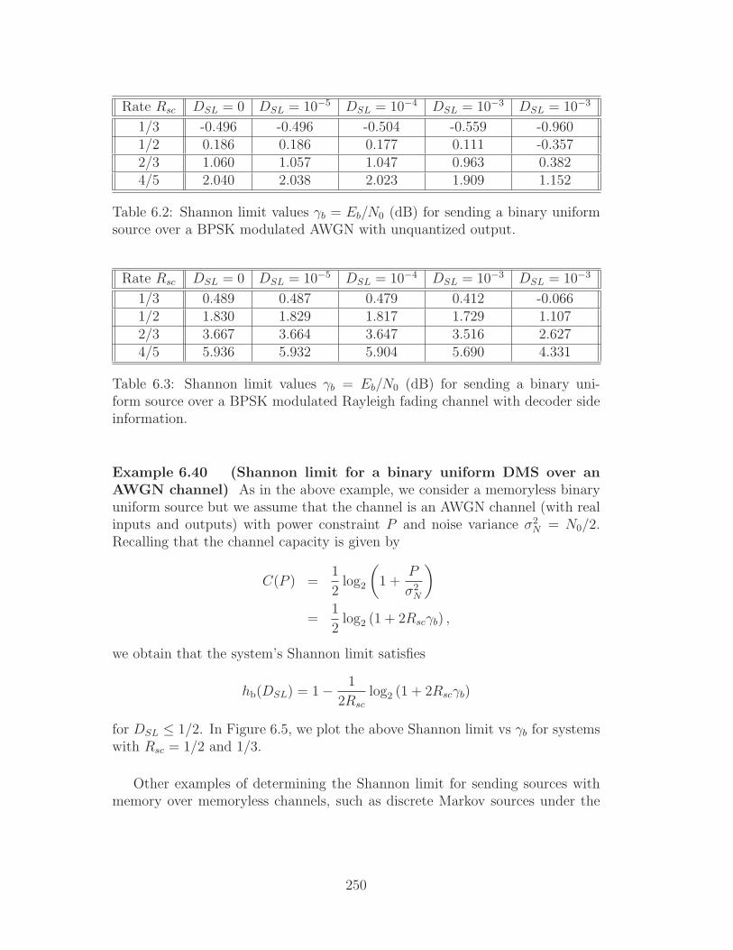
Rate Rsc DSL = 0 DSL = 10−5 DSL = 10−4 DSL = 10−3 DSL = 10−3
1/3 -0.496 -0.496 -0.504 -0.559 -0.9601/2 0.186 0.186 0.177 0.111 -0.3572/3 1.060 1.057 1.047 0.963 0.3824/5 2.040 2.038 2.023 1.909 1.152
Table 6.2: Shannon limit values γb = Eb/N0 (dB) for sending a binary uniformsource over a BPSK modulated AWGN with unquantized output.
Rate Rsc DSL = 0 DSL = 10−5 DSL = 10−4 DSL = 10−3 DSL = 10−3
1/3 0.489 0.487 0.479 0.412 -0.0661/2 1.830 1.829 1.817 1.729 1.1072/3 3.667 3.664 3.647 3.516 2.6274/5 5.936 5.932 5.904 5.690 4.331
Table 6.3: Shannon limit values γb = Eb/N0 (dB) for sending a binary uni-form source over a BPSK modulated Rayleigh fading channel with decoder sideinformation.
Example 6.40 (Shannon limit for a binary uniform DMS over anAWGN channel) As in the above example, we consider a memoryless binaryuniform source but we assume that the channel is an AWGN channel (with realinputs and outputs) with power constraint P and noise variance σ2
N = N0/2.Recalling that the channel capacity is given by
C(P ) =1
2log2
(
1 +P
σ2N
)
=1
2log2 (1 + 2Rscγb) ,
we obtain that the system’s Shannon limit satisfies
hb(DSL) = 1 − 1
2Rsc
log2 (1 + 2Rscγb)
for DSL ≤ 1/2. In Figure 6.5, we plot the above Shannon limit vs γb for systemswith Rsc = 1/2 and 1/3.
Other examples of determining the Shannon limit for sending sources withmemory over memoryless channels, such as discrete Markov sources under the
250

γb (dB)
DSL
Shannon Limit
Rsc = 1/2
Rsc = 1/3
1
10−1
10−2
10−3
10−4
10−5
10−6
−6 −5 −4 −3 −2 −1 −.55−.001 1
Figure 6.5: The Shannon limits for sending a binary uniform sourceover a continuous-input AWGN channel; rates Rsc = 1/2 and 1/3.
Hamming distortion function15 or Gauss-Markov sources under the squared errordistortion measure (e.g., see [69]) can be similarly considered. Finally, we referthe reader to the end of Section 4.5 for a discussion of relevant works on lossyjoint source-channel coding.
Problems
1. Prove Observation 6.15.
2. Binary source with infinite distortion: Let Zi be a DMS with binarysource and reproduction alphabets Z = Z = 0, 1, distribution PZ(1) =p = 1 − PZ(0), where 0 < p ≤ 1/2, and the following distortion measure:
ρ(z, z) =
0 if z = z1 if z = 1 and z = 0∞ if z = 0 and z = 1.
15For example if the Markov source is binary symmetric, then its rate-distortion functionis given by (6.3.9) for D ≤ Dc and the Shannon limit for sending this source over say a BSCor an AWGN channel can be calculated. If the distortion region D > Dc is of interest, then(6.3.8) or the right-side of (6.3.9) can be used as lower bounds on R(D); in this case, a lowerbound on the Shannon limit can be obtained.
251

(a) Determine the source’s rate-distortion function R(D).
(b) Specialize R(D) to the case of p = 1/2 (uniform source).
3. Binary uniform source with erasure and infinite distortion [97]: Considera uniformly distributed DMS Zi with alphabet Z = 0, 1 and repro-duction alphabet Z = 0, 1, E, where E represents an erasure. Let thesource’s distortion function be given as follows:
ρ(z, z) =
0 if z = z1 if z = E∞ otherwise.
Find the source’s rate-distortion function.
4. For the binary source and distortion measure considered in Problem 6.3,describe a simple data compression scheme whose rate achieves the rate-distortion function R(D) for any given distortion threshold D.
5. Non-binary uniform source with erasure and infinite distortion: Considera simple generalization of Problem 6.3 above, where Zi is a uniformlydistributed non-binary DMS with alphabet Z = 0, 1, · · · , q − 1, repro-duction alphabet Z = 0, 1, · · · , q−1, E and the same distortion functionas above, where q ≥ 2 is an integer. Find the source’s rate-distortion func-tion and verify that it reduces to the one derived in Problem 6.3 whenq = 2.
6. Translated distortion [213]: Consider a DMS Zi with alphabet Z andreproduction alphabet Z. Let R(D) denote the source’s rate-distortionfunction under the distortion function ρ(·, ·). Consider a new distortionfunction ρ(·, ·) obtained by adding to ρ(·, ·) a constant that depends on thesource symbols. More specifically, let
ρ(z, z) = ρ(z, z) + cz
where z ∈ Z, z ∈ Z and cz is a constant that depends on source symbol z.Show that the source’s rate-distortion function R(D) associated with thenew distortion function ρ(·, ·) can be expressed as follows in terms of R(D):
R(D) = R(D − c)
for D ≥ c, where c =∑
z∈Z PZ(z)cz.
7. Scaled distortion: Consider a DMS Zi with alphabet Z, reproductionalphabet Z, distortion function ρ(·, ·) and rate-distortion function R(D).
252
Let ρ(·, ·) be a new distortion function obtained by scaling ρ(·, ·) via apositive constant a:
ρ(z, z) = aρ(z, z)
for z ∈ Z and z ∈ Z. Determine the source’s rate-distortion functionR(D) associated with the new distortion function ρ(·, ·) in terms of R(D).
8. Source symbols with zero distortion [213]: Consider a DMS Zi with al-phabet Z, reproduction alphabet Z, distortion function ρ(·, ·) and rate-distortion function R(D). Assume that one source symbol, say z1, in Zhas zero distortion: ρ(z1, z) = 0 for all z ∈ Z. Show that
R(D) = (1 − PZ(z1))R
(D
1 − PZ(z1)
)
where R(D) is the rate-distortion function of source Zi with alphabetZ = Z \ z1 and distribution
PZ(z) =PZ(z)
1 − PZ(z1), z ∈ Z,
and with the same reproduction alphabet Z and distortion function ρ(·, ·).
9. Consider a DMS Zi with quaternary source and reproduction alphabetsZ = Z = 0, 1, 2, 3, probability distribution vector
(PZ(0), PZ(1), PZ(2), PZ(3)) = (p/3, p/3, 1 − p, p/3)
for fixed 0 < p < 1, and distortion measure given by the following matrix
[ρ(z, z)] = [ρzz] =
0 ∞ 1 ∞∞ 0 1 ∞0 0 0 0∞ ∞ 1 0
.
Determine the source’s rate-distortion function.
10. Consider a binary DMS Zi with Z = Z = 0, 1, distribution PZ(0) = p,where 0 < p ≤ 1/2, and the following distortion matrix
[ρ(z, z)] = [ρzz] =
[b1 a + b1
a + b2 b2
]
where a > 0, b1 and b2 are constants.
(a) Find R(D) in terms of a, b1 and b2. (Hint: Use Problems 6.6 and 6.7.)
253

(b) What is R(D) when a = 1 and b1 = b2 = 0 ?
(c) What is R(D) when a = b2 = 1 and b1 = 0 ?
11. Prove Theorem 6.24.
12. Prove Theorem 6.29.
13. Memory decreases the rate distortion function: Give an example of a dis-crete source with memory whose rate-distortion function is strictly less (atleast in some range of the distortion threshold) than the rate-distortionfunction of a memoryless source with identical marginal distribution.
14. Lossy joint source-channel coding theorem - Forward part: Prove the for-ward part of Theorem 6.32. For simplicity assume that the source is mem-oryless.
15. Lossy joint source-channel coding theorem - Converse part: Prove the con-verse part of Theorem 6.32.
16. Gap between the Laplacian rate-distortion function and the Shannon bound:Consider a continuous memoryless source Zi with a pdf of support R,zero mean and E[|Z|] = λ, where λ > 0, under the absolute error distortionmeasure. Show that for any 0 < D ≤ λ,
RL(D) − RLSD(D) = D(Z‖ZL),
where D(Z‖ZL) is the divergence between Z and a Laplacian random vari-able ZL of mean zero and parameter λ, RL(D) denotes the rate-distortionfunction of source ZL (see Theorem 6.28) and RL
SD(D) denotes the Shan-non lower bound under the absolute error distortion measure (see Theo-rem 6.29).
17. q-ary uniform DMS over the q-ary symmetric DMC: Given integer q ≥ 2,consider a q-ary DMS Zn that is uniformly distributed over its alpha-bet Z = 0, 1, · · · , q − 1, with reproduction alphabet Z = Z and theHamming distortion measure. Consider also the q-ary symmetric DMCdescribed in (4.2.11) with q-ary input and output alphabets and symbolerror rate ǫ ≤ q−1
q.
Determine whether or not an uncoded source-channel transmission schemeof rate Rsc = 1 source symbol/channel use (i.e., a source-channel codewhose encoder and decoder are both given by the identity function) isoptimal for this communication system.
254

18. Shannon limit of the erasure source-channel system: Given integer q ≥ 2,consider the q-ary uniform DMS together with the distortion measure ofProblem 6.5 above and the q-ary erasure channel described in (4.2.12), seealso Problem 4.13.
(a) Find the system’s Shannon limit under a transmission rate of Rsc
source symbol/channel use.
(b) Describe an uncoded source-channel transmission scheme for the sys-tem with rate Rsc = 1 and assess its optimality.
19. Shannon limit for a Laplacian source over an AWGN channel: Deter-mine the Shannon limit under the absolute error distortion criterion anda transmission rate of Rsc source symbols/channel use for a communica-tion system consisting of a memoryless zero-mean Laplacian source withparameter λ and an AWGN channel with input power constraint P andnoise variance σ2
N .
20. Shannon limit for a non-uniform DMS over different channels: Find theShannon limit under the Hamming distortion criterion for each of the sys-tems of Examples 6.38, 6.39 and 6.40, where the source is a binary non-uniform DMS with PZ(0) = p, where 0 ≤ p ≤ 1.
255

Appendix A
Overview on Suprema and Limits
We herein review basic results on suprema and limits which are useful for thedevelopment of information theoretic coding theorems; they can be found instandard real analysis texts (e.g., see [186, 282]).
A.1 Supremum and maximum
Throughout, we work on subsets of R, the set of real numbers.
Definition A.1 (Upper bound of a set) A real number u is called an upperbound of a non-empty subset A of R if every element of A is less than or equalto u; we say that A is bounded above. Symbolically, the definition becomes:
A ⊂ R is bounded above ⇐⇒ (∃ u ∈ R) such that (∀ a ∈ A), a ≤ u.
Definition A.2 (Least upper bound or supremum) Suppose A is a non-empty subset of R. Then we say that a real number s is a least upper bound orsupremum of A if s is an upper bound of the set A and if s ≤ s′ for each upperbound s′ of A. In this case, we write s = supA; other notations are s = supx∈A xand s = supx : x ∈ A.
Completeness Axiom: (Least upper bound property) Let A be a non-empty subset of R that is bounded above. Then A has a least upper bound.
It follows directly that if a non-empty set in R has a supremum, then thissupremum is unique. Furthermore, note that the empty set (∅) and any setnot bounded above do not admit a supremum in R. However, when workingin the set of extended real numbers given by R ∪ −∞,∞, we can define the
256
supremum of the empty set as −∞ and that of a set not bounded above as ∞.These extended definitions will be adopted in the text.
We now distinguish between two situations: (i) the supremum of a set Abelongs to A, and (ii) the supremum of a set A does not belong to A. It is quiteeasy to create examples for both situations. A quick example for (i) involvesthe set (0, 1], while the set (0, 1) can be used for (ii). In both examples, thesupremum is equal to 1; however, in the former case, the supremum belongs tothe set, while in the latter case it does not. When a set contains its supremum,we call the supremum the maximum of the set.
Definition A.3 (Maximum) If supA ∈ A, then supA is also called the max-imum of A, and is denoted by maxA. However, if supA 6∈ A, then we say thatthe maximum of A does not exist.
Property A.4 (Properties of the supremum)
1. The supremum of any set in R ∪ −∞,∞ always exits.
2. (∀ a ∈ A) a ≤ supA.
3. If −∞ < supA < ∞, then (∀ ε > 0)(∃ a0 ∈ A) a0 > supA− ε.(The existence of a0 ∈ (supA−ε, supA] for any ε > 0 under the conditionof | supA| < ∞ is called the approximation property for the supremum.)
4. If supA = ∞, then (∀ L ∈ R)(∃ B0 ∈ A) B0 > L.
5. If supA = −∞, then A is empty.
Observation A.5 (Supremum of a set and channel coding theorems) InInformation Theory, a typical channel coding theorem establishes that a (finite)real number α is the supremum of a set A. Thus, to prove such a theorem, onemust show that α satisfies both properties 3 and 2 above, i.e.,
(∀ ε > 0)(∃ a0 ∈ A) a0 > α − ε (A.1.1)
and(∀ a ∈ A) a ≤ α, (A.1.2)
where (A.1.1) and (A.1.2) are called the achievability (or forward) part and theconverse part, respectively, of the theorem. Specifically, (A.1.2) states that α isan upper bound of A, and (A.1.1) states that no number less than α can be anupper bound for A.
257

Property A.6 (Properties of the maximum)
1. (∀ a ∈ A) a ≤ maxA, if maxA exists in R ∪ −∞,∞.
2. maxA ∈ A.
From the above property, in order to obtain α = maxA, one needs to showthat α satisfies both
(∀ a ∈ A) a ≤ α and α ∈ A.
A.2 Infimum and minimum
The concepts of infimum and minimum are dual to those of supremum andmaximum.
Definition A.7 (Lower bound of a set) A real number ℓ is called a lowerbound of a non-empty subset A in R if every element of A is greater than orequal to ℓ; we say that A is bounded below. Symbolically, the definition becomes:
A ⊂ R is bounded below ⇐⇒ (∃ ℓ ∈ R) such that (∀ a ∈ A) a ≥ ℓ.
Definition A.8 (Greatest lower bound or infimum) Suppose A is a non-empty subset of R. Then we say that a real number ℓ is a greatest lower boundor infimum of A if ℓ is a lower bound of A and if ℓ ≥ ℓ′ for each lower boundℓ′ of A. In this case, we write ℓ = inf A; other notations are ℓ = infx∈A x andℓ = infx : x ∈ A.
Completeness Axiom: (Greatest lower bound property) Let A be anon-empty subset of R that is bounded below. Then A has a greatest lowerbound.
As for the case of the supremum, it directly follows that if a non-empty setin R has an infimum, then this infimum is unique. Furthermore, working in theset of extended real numbers, the infimum of the empty set is defined as ∞ andthat of a set not bounded below as −∞.
Definition A.9 (Minimum) If inf A ∈ A, then inf A is also called the min-imum of A, and is denoted by minA. However, if inf A 6∈ A, we say that theminimum of A does not exist.
258
Property A.10 (Properties of the infimum)
1. The infimum of any set in R ∪ −∞,∞ always exists.
2. (∀ a ∈ A) a ≥ inf A.
3. If ∞ > inf A > −∞, then (∀ ε > 0)(∃ a0 ∈ A) a0 < inf A + ε.(The existence of a0 ∈ [inf A, inf A+ε) for any ε > 0 under the assumptionof | inf A| < ∞ is called the approximation property for the infimum.)
4. If inf A = −∞, then (∀A ∈ R)(∃ B0 ∈ A)B0 < L.
5. If inf A = ∞, then A is empty.
Observation A.11 (Infimum of a set and source coding theorems) Anal-ogously to Observation A.5, a typical source coding theorem in Information The-ory establishes that a (finite) real number α is the infimum of a set A. Thus,to prove such a theorem, one must show that α satisfies both properties 3 and 2above, i.e.,
(∀ ε > 0)(∃ a0 ∈ A) a0 < α + ε (A.2.1)
and(∀ a ∈ A) a ≥ α. (A.2.2)
Here, (A.2.1) is called the achievability or forward part of the coding theorem;it specifies that no number greater than α can be a lower bound for A. Also,(A.2.2) is called the converse part of the theorem; it states that α is a lowerbound of A.
Property A.12 (Properties of the minimum)
1. (∀ a ∈ A) a ≥ minA, if minA exists in R ∪ −∞,∞.
2. minA ∈ A.
A.3 Boundedness and suprema operations
Definition A.13 (Boundedness) A subset A of R is said to be bounded if itis both bounded above and bounded below; otherwise it is called unbounded.
Lemma A.14 (Condition for boundedness) A subset A of R is bounded iff(∃ k ∈ R) such that (∀ a ∈ A) |a| ≤ k.
259

Lemma A.15 (Monotone property) Suppose that A and B are non-emptysubsets of R such that A ⊂ B. Then
1. supA ≤ supB.
2. inf A ≥ inf B.
Lemma A.16 (Supremum for set operations) Define the “addition” of twosets A and B as
A + B , c ∈ R : c = a + b for some a ∈ A and b ∈ B.
Define the “scaler multiplication” of a set A by a scalar k ∈ R as
k · A , c ∈ R : c = k · a for some a ∈ A.
Finally, define the “negation” of a set A as
−A , c ∈ R : c = −a for some a ∈ A.
Then the following hold.
1. If A and B are both bounded above, then A + B is also bounded aboveand sup(A + B) = supA + supB.
2. If 0 < k < ∞ and A is bounded above, then k · A is also bounded aboveand sup(k · A) = k · supA.
3. supA = − inf(−A) and inf A = − sup(−A).
Property 1 does not hold for the “product” of two sets, where the “product”of sets A and B is defined as as
A · B , c ∈ R : c = ab for some a ∈ A and b ∈ B.
In this case, both of these two situations can occur:
sup(A · B) > (supA) · (supB)
sup(A · B) = (supA) · (supB).
260
Lemma A.17 (Supremum/infimum for monotone functions)
1. If f : R → R is a non-decreasing function, then
supx ∈ R : f(x) < ε = infx ∈ R : f(x) ≥ ε
andsupx ∈ R : f(x) ≤ ε = infx ∈ R : f(x) > ε.
2. If f : R → R is a non-increasing function, then
supx ∈ R : f(x) > ε = infx ∈ R : f(x) ≤ ε
andsupx ∈ R : f(x) ≥ ε = infx ∈ R : f(x) < ε.
The above lemma is illustrated in Figure A.1.
A.4 Sequences and their limits
Let N denote the set of “natural numbers” (positive integers) 1, 2, 3, · · · . Asequence drawn from a real-valued function is denoted by
f : N → R.
In other words, f(n) is a real number for each n = 1, 2, 3, · · · . It is usual to writef(n) = an, and we often indicate the sequence by any one of these notations
a1, a2, a3, · · · , an, · · · or an∞n=1.
One important question that arises with a sequence is what happens when ngets large. To be precise, we want to know that when n is large enough, whetheror not every an is close to some fixed number L (which is the limit of an).
Definition A.18 (Limit) The limit of an∞n=1 is the real number L satisfying:(∀ ε > 0)(∃ N) such that (∀ n > N)
|an − L| < ε.
In this case, we write L = limn→∞ an. If no such L satisfies the above statement,we say that the limit of an∞n=1 does not exist.
261

-
6
f(x)
ε
supx : f(x) < ε= infx : f(x) ≥ ε
supx : f(x) ≤ ε= infx : f(x) > ε
-
6
f(x)
ε
supx : f(x) ≥ ε= infx : f(x) < ε
supx : f(x) > ε= infx : f(x) ≤ ε
Figure A.1: Illustration of Lemma A.17.
Property A.19 If an∞n=1 and bn∞n=1 both have a limit in R, then the fol-lowing hold.
1. limn→∞(an + bn) = limn→∞ an + limn→∞ bn.
2. limn→∞(α · an) = α · limn→∞ an.
3. limn→∞(anbn) = (limn→∞ an)(limn→∞ bn).
Note that in the above definition, −∞ and ∞ cannot be a legitimate limitfor any sequence. In fact, if (∀ L)(∃ N) such that (∀ n > N) an > L, then we
262

say that an diverges to ∞ and write an → ∞. A similar argument applies toan diverging to −∞. For convenience, we will work in the set of extended realnumbers and thus state that a sequence an∞n=1 that diverges to either ∞ or−∞ has a limit in R ∪ −∞,∞.
Lemma A.20 (Convergence of monotone sequences) If an∞n=1 is non-de-creasing in n, then limn→∞ an exists in R∪−∞,∞. If an∞n=1 is also boundedfrom above – i.e., an ≤ L ∀n for some L in R – then limn→∞ an exists in R.
Likewise, if an∞n=1 is non-increasing in n, then limn→∞ an exists in R ∪−∞,∞. If an∞n=1 is also bounded from below – i.e., an ≥ L ∀n for some Lin R – then limn→∞ an exists in R.
As stated above, the limit of a sequence may not exist. For example, an =(−1)n. Then an will be close to either −1 or 1 for n large. Hence, more general-ized definitions that can describe the general limiting behavior of a sequence isrequired.
Definition A.21 (limsup and liminf) The limit supremum of an∞n=1 is theextended real number in R ∪ −∞,∞ defined by
lim supn→∞
an , limn→∞
(supk≥n
ak),
and the limit infimum of an∞n=1 is the extended real number defined by
lim infn→∞
an , limn→∞
(infk≥n
ak).
Some also use the notations lim and lim to denote limsup and liminf, respectively.
Note that the limit supremum and the limit infimum of a sequence is alwaysdefined in R ∪ −∞,∞, since the sequences supk≥n ak = supak : k ≥ n andinfk≥n ak = infak : k ≥ n are monotone in n (cf. Lemma A.20). An immediateresult follows from the definitions of limsup and liminf.
Lemma A.22 (Limit) For a sequence an∞n=1,
limn→∞
an = L ⇐⇒ lim supn→∞
an = lim infn→∞
an = L.
Some properties regarding the limsup and liminf of sequences (which areparallel to Properties A.4 and A.10) are listed below.
263

Property A.23 (Properties of the limit supremum)
1. The limit supremum always exists in R ∪ −∞,∞.
2. If | lim supm→∞ am| < ∞, then (∀ ε > 0)(∃ N) such that (∀ n > N)an < lim supm→∞ am + ε. (Note that this holds for every n > N .)
3. If | lim supm→∞ am| < ∞, then (∀ ε > 0 and integer K)(∃ N > K) suchthat aN > lim supm→∞ am−ε. (Note that this holds only for one N , whichis larger than K.)
Property A.24 (Properties of the limit infimum)
1. The limit infimum always exists in R ∪ −∞,∞.
2. If | lim infm→∞ am| < ∞, then (∀ ε > 0 and K)(∃ N > K) such thataN < lim infm→∞ am + ε. (Note that this holds only for one N , which islarger than K.)
3. If | lim infm→∞ am| < ∞, then (∀ ε > 0)(∃ N) such that (∀ n > N) an >lim infm→∞ am − ε. (Note that this holds for every n > N .)
The last two items in Properties A.23 and A.24 can be stated using theterminology of sufficiently large and infinitely often, which is often adopted inInformation Theory.
Definition A.25 (Sufficiently large) We say that a property holds for a se-quence an∞n=1 almost always or for all sufficiently large n if the property holdsfor every n > N for some N .
Definition A.26 (Infinitely often) We say that a property holds for a se-quence an∞n=1 infinitely often or for infinitely many n if for every K, the prop-erty holds for one (specific) N with N > K.
Then properties 2 and 3 of Property A.23 can be respectively re-phrased as:if | lim supm→∞ am| < ∞, then (∀ ε > 0)
an < lim supm→∞
am + ε for all sufficiently large n
andan > lim sup
m→∞am − ε for infinitely many n.
264

Similarly, properties 2 and 3 of Property A.24 becomes: if | lim infm→∞ am| < ∞,then (∀ ε > 0)
an < lim infm→∞
am + ε for infinitely many n
andan > lim inf
m→∞am − ε for all sufficiently large n.
Lemma A.27
1. lim infn→∞ an ≤ lim supn→∞ an.
2. If an ≤ bn for all sufficiently large n, then
lim infn→∞
an ≤ lim infn→∞
bn and lim supn→∞
an ≤ lim supn→∞
bn.
3. lim supn→∞ an < r ⇒ an < r for all sufficiently large n.
4. lim supn→∞ an > r ⇒ an > r for infinitely many n.
5.
lim infn→∞
an + lim infn→∞
bn ≤ lim infn→∞
(an + bn)
≤ lim supn→∞
an + lim infn→∞
bn
≤ lim supn→∞
(an + bn)
≤ lim supn→∞
an + lim supn→∞
bn.
6. If limn→∞ an exists, then
lim infn→∞
(an + bn) = limn→∞
an + lim infn→∞
bn
andlim sup
n→∞(an + bn) = lim
n→∞an + lim sup
n→∞bn.
Finally, one can also interpret the limit supremum and limit infimum in termsof the concept of clustering points. A clustering point is a point that a sequencean∞n=1 approaches (i.e., belonging to a ball with arbitrarily small radius andthat point as center) infinitely many times. For example, if an = sin(nπ/2),then an∞n=1 = 1, 0,−1, 0, 1, 0,−1, 0, . . .. Hence, there are three clusteringpoints in this sequence, which are −1, 0 and 1. Then the limit supremum ofthe sequence is nothing but its largest clustering point, and its limit infimumis exactly its smallest clustering point. Specifically, lim supn→∞ an = 1 andlim infn→∞ an = −1. This approach can sometimes be useful to determine thelimsup and liminf quantities.
265

A.5 Equivalence
We close this appendix by providing some equivalent statements that are oftenused to simplify proofs. For example, instead of directly showing that quantityx is less than or equal to quantity y, one can take an arbitrary constant ε > 0and prove that x < y + ε. Since y + ε is a larger quantity than y, in some casesit might be easier to show x < y + ε than proving x ≤ y. By the next theorem,any proof that concludes that “x < y + ε for all ε > 0” immediately gives thedesired result of x ≤ y.
Theorem A.28 For any x, y and a in R,
1. x < y + ε for all ε > 0 iff x ≤ y;
2. x < y − ε for some ε > 0 iff x < y;
3. x > y − ε for all ε > 0 iff x ≥ y;
4. x > y + ε for some ε > 0 iff x > y;
5. |a| < ε for all ε > 0 iff a = 0.
266

Appendix B
Overview in Probability and RandomProcesses
This appendix presents a quick overview of basic concepts from probability the-ory and the theory of random processes. The reader can consult comprehensivetexts on these subjects for a thorough study (see, e.g., [19, 32, 120]). We closethe appendix with a brief discussion of Jensen’s inequality and the Lagrangemultipliers technique for the optimization of convex functions [31, 38].
B.1 Probability space
Definition B.1 (σ-Fields) Let F be a collection of subsets of a non-empty setΩ. Then F is called a σ-field (or σ-algebra) if the following hold:
1. Ω ∈ F .
2. Closedness of F under complementation: If A ∈ F , then Ac ∈ F , whereAc = ω ∈ Ω : ω 6∈ A.
3. Closedness of F under countable union: If Ai ∈ F for i = 1, 2, 3, . . ., then⋃∞
i=1 Ai ∈ F .
It directly follows that the empty set ∅ is also an element of F (as Ωc = ∅)and that F is closed under countable intersection since
∞⋂
i=1
Aci =
( ∞⋃
i=1
Ai
)c
.
The largest σ-field of subsets of a given set Ω is the collection of all subsets ofΩ (i.e., its powerset), while the smallest σ-field is given by Ω, ∅. Also, if A is
267

a proper (strict) non-empty subset of Ω, then the smallest σ-field containing Ais given by Ω, ∅, A,Ac.
Definition B.2 (Probability space) A probability space is a triple (Ω,F , P ),where Ω is a given set called sample space containing all possible outcomes(usually observed from an experiment), F is a σ-field of subsets of Ω and Pis a probability measure P : F → [0, 1] on the σ-field satisfying the following:
1. 0 ≤ P (A) ≤ 1 for all A ∈ F .
2. P (Ω) = 1.
3. Countable additivity: If A1, A2, . . . is a sequence of disjoint sets (i.e.,Ai ∩ Aj = ∅ for all i 6= j) in F , then
P
( ∞⋃
k=1
Ak
)
=∞∑
k=1
P (Ak).
It directly follows from properties 1-3 of the above definition that P (∅) = 0.Usually, the σ-field F is called the event space and its elements (which aresubsets of Ω satisfying the properties of Definition B.1) are called events.
B.2 Random variable and random process
A random variable X defined over probability space (Ω,F , P ) is a real-valuedfunction X : Ω → R that is measurable (or F-measurable), i.e., satisfying theproperty that
X−1((−∞, t]) , ω ∈ Ω : X(ω) ≤ t ∈ Ffor each real t.1
A random process is a collection of random variables that arise from the sameprobability space. It can be mathematically represented by the collection
Xt, t ∈ I,
1One may question why bother defining random variables based on some abstract proba-bility space. One may continue “A random variable X can simply be defined based on itsdistribution PX ,” which is indeed true (cf. Section B.3).
A perhaps easier way to understand the abstract definition of random variables is that theunderlying probability space (Ω,F , P ) on which the random variable is defined is what trulyoccurs internally, but it is possibly non-observable. In order to infer which of the non-observableω occurs, an experiment that results in observable x that is a function of ω is performed. Suchan experiment results in the random variable X whose probability is so defined over theprobability space (Ω,F , P ).
268

where Xt denotes the tth random variable in the process, and the index t runsover an index set I which is arbitrary. The index set I can be uncountably infinite— e.g., I = R — in which case we are effectively dealing with a continuous-timeprocess. We will however exclude such a case in this chapter for the sake ofsimplicity. To be precise, we will only consider the following cases of index setI:
case a) I consists of one index only.case b) I is finite.case c) I is countably infinite.
B.3 Distribution functions versus probability space
In applications, we are perhaps more interested in the distribution functionsof the random variables and random processes than the underlying probabilityspace on which the random variables and random processes are defined. It canbe proved [32, Thm. 14.1] that given a real-valued non-negative function F (·)that is non-decreasing and right-continuous and satisfies limx↓−∞ F (x) = 0 andlimx↑∞ F (x) = 1, there exist a random variable and an underlying probabilityspace such that the cumulative distribution function (cdf) of the random variabledefined over the probability space is equal to F (·). This result releases us fromthe burden of referring to a probability space before defining the random variable.In other words, we can define a random variable X directly by its cdf, i.e., Pr[X ≤x], without bothering to refer to its underlying probability space. Nevertheless,it is better to keep in mind (and learn) that, formally, random variables andrandom processes are defined over underlying probability spaces.
B.4 Relation between a source and a random process
In statistical communication, a discrete-time source (X1, X2, X3, . . . , Xn) , Xn
consists of a sequence of random quantities, where each quantity usually takeson values from a source generic alphabet X , namely
(X1, X2, . . . , Xn) ∈ X × X × · · · × X , X n.
Another merit in defining random variables based on an abstract probability space can beobserved from the extension definition of random variables to random processes. With theunderlying probability space, any finite dimensional distribution of Xt, t ∈ I is well-defined.For example,
Pr[X1 ≤ x1,X5 ≤ x5,X9 ≤ x9] = P (ω ∈ Ω : X1(ω) ≤ x1,X5(ω) ≤ x5,X9(ω) ≤ x9) .
269

The elements in X are usually called letters.
B.5 Statistical properties of random sources
For a random process X = X1, X2, . . . with alphabet X (i.e., X ⊆ R is therange of each Xi) defined over probability space (Ω,F , P ), consider X∞, the setof all sequences x , (x1, x2, x3, . . .) of real numbers in X . An event E in2 FX, thesmallest σ-field generated by all open sets of X∞ (i.e., the Borel σ-field of X∞),is said to be T-invariant with respect to the left-shift (or shift transformation)T : X∞ → X∞ if
TE ⊆ E,
where
TE , Tx : x ∈ E and Tx , T(x1, x2, x3, . . .) = (x2, x3, . . .).
In other words, T is equivalent to “chopping the first component.” For example,applying T onto an event E1 defined below,
E1 , (x1 = 1, x2 = 1, x3 = 1, x4 = 1, . . .), (x1 = 0, x2 = 1, x3 = 1, x4 = 1, . . .),
(x1 = 0, x2 = 0, x3 = 1, x4 = 1, . . .) , (B.5.1)
yields
TE1 = (x1 = 1, x2 = 1, x3 = 1, . . .), (x1 = 1, x2 = 1, x3 = 1 . . .),
(x1 = 0, x2 = 1, x3 = 1, . . .)= (x1 = 1, x2 = 1, x3 = 1, . . .), (x1 = 0, x2 = 1, x3 = 1, . . .) .
We then have TE1 ⊆ E1, and hence E1 is T-invariant.
It can be proved3 that if TE ⊆ E, then T2E ⊆ TE. By induction, we canfurther obtain
· · · ⊆ T3E ⊆ T2E ⊆ TE ⊆ E.
Thus, if an element say (1, 0, 0, 1, 0, 0, . . .) is in a T-invariant set E, then all itsleft-shift counterparts (i.e., (0, 0, 1, 0, 0, 1 . . .) and (0, 1, 0, 0, 1, 0, . . .)) should becontained in E. As a result, for a T-invariant set E, an element and all its left-shift counterparts are either all in E or all outside E, but cannot be partiallyinside E. Hence, a “T-invariant group” such as one containing (1, 0, 0, 1, 0, 0, . . .),
2Note that by definition, the events E ∈ FX are measurable, and PX(E) = P (A), wherePX is the distribution of X induced from the underlying probability measure P .
3If A ⊆ B, then TA ⊆ TB. Thus T2E ⊆ TE holds whenever TE ⊆ E.
270

(0, 0, 1, 0, 0, 1 . . .) and (0, 1, 0, 0, 1, 0, . . .) should be treated as an indecomposablegroup in T-invariant sets.
Although we are in particular interested in these “T-invariant indecomposablegroups” (especially when defining an ergodic random process), it is possible thatsome single “transient” element, such as (0, 0, 1, 1, . . .) in (B.5.1), is includedin a T-invariant set, and will be excluded after applying left-shift operation T.This however can be resolved by introducing the inverse operation T−1. Notethat T is a many-to-one mapping, so its inverse operation does not exist ingeneral. Similar to taking the closure of an open set, the definition adoptedbelow [248, p. 3] allows us to “enlarge” the T-invariant set such that all right-shift counterparts of the single “transient” element are included.
T−1E , x ∈ X∞ : Tx ∈ E .
We then notice from the above definition that if
T−1E = E, (B.5.2)
then4
TE = T(T−1E) = E,
and hence E is constituted only by the T-invariant groups because
· · · = T−2E = T−1E = E = TE = T2E = · · · .
The sets that satisfy (B.5.2) are sometimes referred to as ergodic sets becauseas time goes by (the left-shift operator T can be regarded as a shift to a futuretime), the set always stays in the state that it has been before. A quick exampleof an ergodic set for X = 0, 1 is one that consists of all binary sequences thatcontain finitely many 0’s.5
We now classify several useful statistical properties of random process X =X1, X2, . . ..
4The proof of T(T−1E) = E is as follows. If y ∈ T(T−1E) = T(x ∈ X∞ : Tx ∈ E), thenthere must exist an element x ∈ x ∈ X∞ : Tx ∈ E such that y = Tx. Since Tx ∈ E, wehave y ∈ E and T(T−1E) ⊆ E.
On the contrary, if y ∈ E, all x’s satisfying Tx = y belong to T−1E. Thus, y ∈ T(T−1E),which implies E ⊆ T(T−1E).
5As the textbook only deals with one-sided random processes, the discussion on T-invariance only focuses on sets of one-sided sequences. When a two-sided random process. . . ,X−2,X−1,X0,X1,X2, . . . is considered, the left-shift operation T of a two-sided sequenceactually has a unique inverse. Hence, TE ⊆ E implies TE = E. Also, TE = E if, andonly if, T−1E = E. Ergodicity for two-sided sequences can therefore be directly defined usingTE = E.
271
• Memoryless: A random process is said to be memoryless if the sequence ofrandom variables Xi is independent and identically distributed (i.i.d.).
• First-order stationary: A process is first-order stationary if the marginaldistribution is unchanged for every time instant.
• Second-order stationary: A process is second-order stationary if the jointdistribution of any two (not necessarily consecutive) time instances is in-variant before and after left (time) shift.
• Weakly stationary process: A process is weakly stationary (or wide-sensestationary or stationary in the weak or wide sense) if the mean and auto-correlation function are unchanged by a left (time) shift.
• Stationary process: A process is stationary (or strictly stationary) if theprobability of every sequence or event is unchanged by a left (time) shift.
• Ergodic process: A process is ergodic if any ergodic set (satisfying (B.5.2))in FX has probability either 1 or 0. This definition is not very intuitive,but some interpretations and examples may shed some light.
Observe that the definition has nothing to do with stationarity. Itsimply states that events that are unaffected by time-shifting (both left-and right-shifting) must have probability either zero or one.
Ergodicity implies that all convergent sample averages6 converge to aconstant (but not necessarily to the ensemble average), and stationarityassures that the time average converges to a random variable; hence, itis reasonably to expect that they jointly imply the ultimate time averageequals the ensemble average. This is validated by the well-known ergodictheorem by Birkhoff and Khinchin.
Theorem B.3 (Pointwise ergodic theorem) Consider a discrete-timestationary random process, X = Xn∞n=1. For real-valued function f(·) onR with finite mean (i.e., |E[f(Xn)]| < ∞), there exists a random variableY such that
limn→∞
1
n
n∑
k=1
f(Xk) = Y with probability 1.
If, in addition to stationarity, the process is also ergodic, then
limn→∞
1
n
n∑
k=1
f(Xk) = E[f(X1)] with probability 1.
6Two alternative names for sample average are time average and Cesaro mean. In thisbook, these names will be used interchangeably.
272

Example B.4 Consider the process Xi∞i=1 consisting of a family of i.i.d. bi-nary random variables (obviously, it is stationary and ergodic). Define thefunction f(·) by f(0) = 0 and f(1) = 1, Hence,7
E[f(Xn)] = PXn(0)f(0) + PXn(1)f(1) = PXn(1)
is finite. By the pointwise ergodic theorem, we have
limn→∞
f(X1) + f(X2) + · · · + f(Xn)
n= lim
n→∞
X1 + X2 + · · · + Xn
n= PX(1).
As seen in the above example, one of the important consequencesthat the pointwise ergodic theorem indicates is that the time average canultimately replace the statistical average, which is a useful result in engi-neering. Hence, with stationarity and ergodicity, one, who observes
X301 = 154326543334225632425644234443
from the experiment of rolling a dice, can draw the conclusion that thetrue distribution of rolling the dice can be well approximated by:
PrXi = 1 ≈ 1
30PrXi = 2 ≈ 6
30PrXi = 3 ≈ 7
30
PrXi = 4 ≈ 9
30PrXi = 5 ≈ 4
30PrXi = 6 ≈ 3
30
Such result is also known by the law of large numbers. The relation be-tween ergodicity and the law of large numbers will be further explored inSection B.7.
We close the discussion on ergodicity by remarking that in communica-tions theory, one may assume that the source is stationary or the source isstationary ergodic. But it is rare to see the assumption of the source beingergodic but non-stationary. This is perhaps because an ergodic but non-stationary source not only does not facilitate the analytical study of com-munications problems, but may have limited application in practice. Fromthis, we note that assumptions are made either to facilitate the analyticalstudy of communications problems or to fit a specific need of applications.Without these two objectives, an assumption becomes of minor interest.This, to some extent, justifies that the ergodicity assumption usually comesafter stationarity assumption. A specific example is the pointwise ergodictheorem, where the random processes considered is presumed to be sta-tionary.
7In terms of notation, we use PXn(0) to denote PrXn = 0. The above two representations
will be used alternatively throughout the book.
273

• First-order Markov chain: Three random variables X, Y and Z are saidto form a Markov chain or a first-order Markov chain if
PX,Y,Z(x, y, z) = PX(x) · PY |X(y|x) · PZ|Y (z|y); (B.5.3)
i.e., PZ|X,Y (z|x, y) = PZ|Y (z|y). This is usually denoted by X → Y → Z.
X → Y → Z is sometimes read as “ X and Z are conditionally independentgiven Y ” because it can be shown that (B.5.3) is equivalent to
PX,Z|Y (x, z|y) = PX|Y (x|y) · PZ|Y (z|y).
Therefore, X → Y → Z is equivalent to Z → Y → X. Accordingly, theMarkovian notation is sometimes expressed as X ↔ Y ↔ Z.
• Markov chain for random sequences: The sequence of random variablesX1, X2, X3, . . . with common finite-alphabet X are said to form a k-thorder Markov chain if for all k < n,
Pr[Xn = xn|Xn−1 = xn−1, . . . , X1 = x1]
= Pr[Xn = xn|Xn−1 = xn−1, . . . , Xn−k = xn−k].
Each xn−1n−k ∈ X k is called the state at time n.
– A k-th order Markov chain is irreducible if with some probability, wecan go from any state in X k to another state in a finite number ofsteps, i.e., for all xk, yk ∈ X k there exists an integer j ≥ 1 such that
Pr
Xk+j−1j = xk
∣∣∣Xk
1 = yk
> 0.
– A k-th order Markov chain is said to be time-invariant or homoge-neous, if for every n > k,
Pr[Xn = xn|Xn−1 = xn−1, . . . , Xn−k = xn−k]
= Pr[Xk+1 = xk+1|Xk = xk, . . . , X1 = x1].
Therefore, a homogeneous first-order Markov chain can be definedthrough its transition probability:
[PrX2 = x2|X1 = x1
]
|X |×|X |,
and its initial state distribution PX1(x).
274

– In a first-order Markov chain, the period d(x) of state x ∈ X is definedby
d(x) , gcd n ∈ 1, 2, 3, · · · : PrXn+1 = x|X1 = x > 0 ,
where gcd denotes the greatest common divisor; in other words, ifthe Markov chain starts in state x, then the chain cannot return tostate x at any time that is not a multiple of d(x). If PrXn+1 =x|X1 = x = 0 for all n, we say that state x has an infinite periodand write d(x) = ∞. We also say that state x is aperiodic if d(x) = 1and periodic if d(x) > 1. Furthermore, the first-order Markov chainis called aperiodic if all its states are aperiodic. In other words, thefirst-order Markov chain is aperiodic if
gcd n ∈ 1, 2, 3, · · · : PrXn+1 = x|X1 = x > 0 = 1 ∀x ∈ X .
– In an irreducible first-order Markov chain, all states have the sameperiod. Hence, if one state in such a chain is aperiodic, then the entireMarkov chain is aperiodic.
– A distribution π(·) on X is said to be a stationary distribution for ahomogeneous first-order Markov chain, if for every y ∈ X ,
π(y) =∑
x∈Xπ(x) PrX2 = y|X1 = x.
For a finite-alphabet homogeneous first-order Markov chain, π(·) al-ways exists; furthermore, π(·) is unique if the Markov chain is irre-ducible. For a finite-alphabet homogeneous first-order Markov chainthat is both irreducible and aperiodic,
limn→∞
PrXn+1 = y|X1 = x = π(y)
for all states x and y in X . If the initial state distribution is equal toa stationary distribution, then the homogeneous first-order Markovchain becomes a stationary process.
The general relations among i.i.d. sources, Markov sources, stationary sourcesand ergodic sources are depicted in Figure B.1
B.6 Convergence of sequences of random variables
In this section, we will discuss modes in which a random process X1, X2, . . .converges to a limiting random variable X. Recall that a random variable is a
275

Markov
i.i.d. Stationary
Ergodic
Figure B.1: General relations of random processes.
real-valued function from Ω to R, where Ω the sample space of the probabilityspace over which the random variable is defined. So the following two expressionswill be used interchangeably.
X1(ω), X2(ω), X3(ω), . . . ≡ X1, X2, X3, . . .
for ω ∈ Ω. Note that the random variables in a random process are defined overthe same probability space (Ω,F , P ),
Definition B.5 (Convergence modes for random sequences)
1. Point-wise convergence on Ω.8
Xn∞n=1 is said to converge to X pointwisely on Ω if
limn→∞
Xn(ω) = X(ω) for all ω ∈ Ω.
This is usually denoted by Xnp.w.−→ X.
2. Almost sure convergence or convergence with probability 1.
Xn∞n=1 is said to converge to X with probability 1, if
Pω ∈ Ω : limn→∞
Xn(ω) = X(ω) = 1.
8Although such mode of convergence is not used in probability theory, we introduce itherein to contrast it with the almost sure convergence mode (see Example B.6).
276

This is usually denoted by Xna.s.−→ X.
3. Convergence in probability.
Xn∞n=1 is said to converge to X in probability, if for any ε > 0,
limn→∞
Pω ∈ Ω : |Xn(ω) − X(ω)| > ε = limn→∞
Pr|Xn − X| > ε = 0.
This is usually denoted by Xnp−→ X.
4. Convergence in rth mean.
Xn∞n=1 is said to converge to X in rth mean, if
limn→∞
E[|X − Xn|r] = 0.
This is usually denoted by XnLr−→ X.
5. Convergence in distribution.
Xn∞n=1 is said to converge to X in distribution, if
limn→∞
FXn(x) = FX(x),
for every continuity point of F (x), where
FXn(x) , PrXn ≤ x and FX(x) , PrX ≤ x.
This is usually denoted by Xnd−→ X.
An example that facilitates the understanding of pointwise convergence andalmost sure convergence is as follows.
Example B.6 Give a probability space (Ω, 2Ω, P ), where Ω = 0, 1, 2, 3, andP (0) = P (1) = P (2) = 1/3 and P (3) = 0. Define a random variable as Xn(ω) =ω/n. Then
PrXn = 0 = Pr
Xn =1
n
= Pr
Xn =2
n
=1
3.
It is clear that for every ω in Ω, Xn(ω) converges to X(ω), where X(ω) = 0 forevery ω ∈ Ω; so
Xnp.w.−→ X.
Now let X(ω) = 0 for ω = 0, 1, 2 and X(ω) = 1 for ω = 3. Then both of thefollowing statements are true:
Xna.s.−→ X and Xn
a.s.−→ X,
277

since
Pr
limn→∞
Xn = X
=3∑
ω=0
P (ω) · 1
limn→∞
Xn(ω) = X(ω)
= 1,
where 1· represents the set indicator function. However, Xn does not convergeto X pointwise because limn→∞ Xn(3) 6= X(3). So to speak, pointwise conver-gence requires “equality” even for those samples without probability mass, forwhich almost surely convergence does not take into consideration.
Observation B.7 (Uniqueness of convergence)
1. If Xnp.w.−→ X and Xn
p.w.−→ Y , then X = Y pointwisely. I.e., (∀ ω ∈ Ω)X(ω) = Y (ω).
2. If Xna.s.−→ X and Xn
a.s.−→ Y (or Xnp−→ X and Xn
p−→ Y ) (or XnLr−→ X
and XnLr−→ Y ), then X = Y with probability 1. I.e., PrX = Y = 1.
3. Xnd−→ X and Xn
d−→ Y , then FX(x) = FY (x) for all x.
For ease of understanding, the relations of the five modes of convergence canbe depicted as follows. As usual, a double arrow denotes implication.
-Thm. B.9
Thm. B.8
Xnp.w.−→ X⇓
Xna.s.−→ X Xn
Lr−→ X (r ≥ 1)
Xnp−→ X⇓
Xnd−→ X
There are some other relations among these five convergence modes that arealso depicted in the above graph (via the dotted line); they are stated below.
Theorem B.8 (Monotone convergence theorem [32])
Xna.s.−→ X, (∀ n)Y ≤ Xn ≤ Xn+1, and E[|Y |] < ∞ ⇒ Xn
L1−→ X
⇒ E[Xn] → E[X].
278

Theorem B.9 (Dominated convergence theorem [32])
Xna.s.−→ X, (∀ n)|Xn| ≤ Y, and E[|Y |] < ∞ ⇒ Xn
L1−→ X
⇒ E[Xn] → E[X].
The implication of XnL1−→ X to E[Xn] → E[X] can be easily seen from
|E[Xn] − E[X]| = |E[Xn − X]| ≤ E[|Xn − X|].
B.7 Ergodicity and laws of large numbers
B.7.1 Laws of large numbers
Consider a random process X1, X2, . . . with common marginal mean µ. Supposethat we wish to estimate µ on the basis of the observed sequence x1, x2, x3, . . . .The weak and strong laws of large numbers ensure that such inference is possible(with reasonable accuracy), provided that the dependencies between Xn’s aresuitably restricted: e.g., the weak law is valid for uncorrelated Xn’s, while thestrong law is valid for independent Xn’s. Since independence is a more restrictivecondition than the absence of correlation, one expects the strong law to be morepowerful than the weak law. This is indeed the case, as the weak law states thatthe sample average
X1 + · · · + Xn
n
converges to µ in probability, while the strong law asserts that this convergencetakes place with probability 1.
The following two inequalities will be useful in the discussion of this subject.
Lemma B.10 (Markov’s inequality) For any integer k > 0, real numberα > 0 and any random variable X,
Pr[|X| ≥ α] ≤ 1
αkE[|X|k].
Proof: Let FX(·) be the cdf of random variable X. Then,
E[|X|k] =
∫ ∞
−∞|x|kdFX(x)
≥∫
x∈R : |x|≥α|x|kdFX(x)
279

≥∫
x∈R : |x|≥ααkdFX(x)
= αk
∫
x∈R : |x|≥αdFX(x)
= αk Pr[|X| ≥ α].
Equality holds iff∫
x∈R : |x|<α|x|kdFX(x) = 0 and
∫
x∈R : |x|>α|x|kdFX(x) = 0,
namely,Pr[X = 0] + Pr[|X| = α] = 1.
2
In the proof of Markov’s inequality, we use the general representation forintegration with respect to a (cumulative) distribution function FX(·), i.e.,
∫
X·dFX(x), (B.7.1)
which is named the Lebesgue-Stieltjes integral. Such a representation can beapplied for both discrete and continuous supports as well as the case that theprobability density function does not exist. We use this notational convention toremove the burden of differentiating discrete random variables from continuousones.
Lemma B.11 (Chebyshev’s inequality) For any random variable X and realnumber α > 0,
Pr[|X − E[X]| ≥ α] ≤ 1
α2Var[X].
Proof: By Markov’s inequality with k = 2, we have:
Pr[|X − E[X]| ≥ α] ≤ 1
α2E[|X − E[X]|2].
Equality holds iff
Pr[|X − E[X]| = 0] + Pr[|X − E[X]| = α
]= 1,
equivalently, there exists p ∈ [0, 1] such that
Pr[X = E[X] + α
]= Pr
[X = E[X] − α
]= p and Pr[X = E[X]] = 1 − 2p.
2
In the proofs of the above two lemmas, we also provide the condition underwhich equality holds. These conditions indicate that equality usually cannot befulfilled. Hence in most cases, the two inequalities are strict.
280

Theorem B.12 (Weak law of large numbers) Let Xn∞n=1 be a sequenceof uncorrelated random variables with common mean E[Xi] = µ. If the variablesalso have common variance, or more generally,
limn→∞
1
n2
n∑
i=1
Var[Xi] = 0, (equivalently,X1 + · · · + Xn
n
L2−→ µ)
then the sample averageX1 + · · · + Xn
n
converges to the mean µ in probability.
Proof: By Chebyshev’s inequality,
Pr
∣∣∣∣∣
1
n
n∑
i=1
Xi − µ
∣∣∣∣∣≥ ε
≤ 1
n2ε2
n∑
i=1
Var[Xi].
2
Note that the right-hand side of the above Chebyshev’s inequality is just thesecond moment of the difference between the n-sample average and the mean
µ. Thus the variance constraint is equivalent to the statement that XnL2−→ µ
implies Xnp−→ µ.
Theorem B.13 (Kolmogorov’s strong law of large numbers) Let Xn∞n=1
be an independent sequence of random variables with common mean E[Xn] = µ.If either
1. Xn’s are identically distributed; or
2. Xn’s are square-integrable9 with
∞∑
i=1
Var[Xi]
i2< ∞,
thenX1 + · · · + Xn
n
a.s.−→ µ.
9A random variable X is said to be square-integrable if E[|X|2] < ∞.
281

Note that the above i.i.d. assumption does not exclude the possibility ofµ = ∞ (or µ = −∞), in which case the sample average converges to ∞ (or −∞)with probability 1. Also note that there are cases of independent sequences towhich the weak law applies, but the strong law does not. This is due to the factthat
n∑
i=1
Var[Xi]
i2≥ 1
n2
n∑
i=1
Var[Xi].
The final remark is that Kolmogorov’s strong law of large number can beextended to a function of an independent sequence of random variables:
g(X1) + · · · + g(Xn)
n
a.s.−→ E[g(X1)].
But such extension cannot be applied to the weak law of large number, sinceg(Yi) and g(Yj) can be correlated even if Yi and Yi are not.
B.7.2 Ergodicity and law of large numbers
After the introduction of Kolmogorov’s strong law of large numbers, one may findthat the pointwise ergodic theorem (Theorem B.3) actually indicates a similarresult. In fact, the pointwise ergodic theorem can be viewed as another versionof strong law of large numbers, which states that for stationary and ergodicprocesses, time averages converge with probability 1 to the ensemble expectation.
The notion of ergodicity is often misinterpreted, since the definition is notvery intuitive. Some engineering texts may provide a definition that a stationaryprocess satisfying the ergodic theorem is also ergodic.10 However, the ergodictheorem is indeed a consequence of the original mathematical definition of ergod-icity in terms of the shift-invariant property (see Section B.5 and the discussionin [118, pp. 174-175])).
Let us try to clarify the notion of ergodicity by the following remarks.
10Here is one example. A stationary random process Xn∞n=1 is called ergodic if for arbitraryinteger k and function f(·) on X k of finite mean,
1
n
n∑
i=1
f(Xi+1, . . . ,Xi+k)a.s.−→ E[f(X1, . . . ,Xk)].
As a result of this definition, a stationary ergodic source is the most general dependent randomprocess for which the strong law of large numbers holds. This definition somehow implies thatif a process is not stationary-ergodic, then the strong law of large numbers is violated (orthe time average does not converge with probability 1 to its ensemble expectation). But thisis not true. One can weaken the conditions of stationarity and ergodicity from its originalmathematical definitions to asymptotic stationarity and ergodicity, and still make the stronglaw of large numbers hold. (Cf. the last remark in this section and also Figure B.2)
282

Ergodicitydefined throughshift-invariance
property
Ergodicitydefined throughergodic theorem
i.e., stationarity andtime averageconverging to
sample average(law of large numbers)
Figure B.2: Relation of ergodic random processes respectively definedthrough time-shift invariance and ergodic theorem.
• The concept of ergodicity does not require stationarity. In other words, anon-stationary process can be ergodic.
• Many perfectly good models of physical processes are not ergodic, yet theyhave a form of law of large numbers. In other words, non-ergodic processescan be perfectly good and useful models.
• There is no finite-dimensional equivalent definition of ergodicity as there isfor stationarity. This fact makes it more difficult to describe and interpretergodicity.
• I.i.d. processes are ergodic; hence, ergodicity can be thought of as a (kindof) generalization of i.i.d.
• As mentioned earlier, stationarity and ergodicity imply the time averageconverges with probability 1 to the ensemble mean. Now if a processis stationary but not ergodic, then the time average still converges, butpossibly not to the ensemble mean.
For example, let An∞n=−∞ and Bn∞n=−∞ be two i.i.d. binary 0-1random variables with PrAn = 0 = PrBn = 1 = 1/4. Suppose thatXn = An if U = 1, and Xn = Bn if U = 0, where U is equiprobable binaryrandom variable, and An∞n=1, Bn∞n=1 and U are independent. ThenXn∞n=1 is stationary. Is the process ergodic? The answer is negative.If the stationary process were ergodic, then from the pointwise ergodictheorem (Theorem B.3), its relative frequency would converge to
Pr(Xn = 1) = Pr(U = 1) Pr(Xn = 1|U = 1)
283

+ Pr(U = 0) Pr(Xn = 1|U = 0)
= Pr(U = 1) Pr(An = 1) + Pr(U = 0) Pr(Bn = 1) =1
2.
However, one should observe that the outputs of (X1, . . . , Xn) form aBernoulli process with relative frequency of 1’s being either 3/4 or 1/4,depending on the value of U . Therefore,
limn→∞
1
n
n∑
i=1
Xna.s.−→ Y,
where Pr(Y = 1/4) = Pr(Y = 3/4) = 1/2, which contradicts to the ergodictheorem.
From the above example, the pointwise ergodic theorem can actuallybe made useful in such a stationary but non-ergodic case, since the esti-mate with stationary ergodic process (either An∞n=−∞ or Bn∞n=−∞) isactually being observed by measuring the relative frequency (3/4 or 1/4).This renders a surprising fundamental result of random processes— er-godic decomposition theorem: under fairly general assumptions, any (notnecessarily ergodic) stationary process is in fact a mixture of stationaryergodic processes, and hence one always observes a stationary ergodic out-come. As in the above example, one always observe either A1, A2, A3, . . .or B1, B2, B3, . . ., depending on the value of U , for which both sequencesare stationary ergodic (i.e., the time-stationary observation Xn satisfiesXn = U · An + (1 − U) · Bn).
• The previous remark implies that ergodicity is not required for the str-ong law of large numbers to be useful. The next question is whether ornot stationarity is required. Again the answer is negative. In fact, themain concern of the law of large numbers is the convergence of sampleaverages to its ensemble expectation. It should be reasonable to expectthat random processes could exhibit transient behavior that violates thestationarity definition, yet the sample average still converges. One canthen introduce the notion of asymptotically stationary to achieve the lawof large numbers. For example, a finite-alphabet time-invariant (but notnecessarily stationary) irreducible Markov chain satisfies the law of largenumbers.
Accordingly, one should not take the notions of stationarity and er-godicity too seriously (if the main concern is the law of large numbers)since they can be significantly weakened and still have laws of large num-bers holding (i.e., time averages and relative frequencies have desired andwell-defined limits).
284
B.8 Central limit theorem
Theorem B.14 (Central limit theorem) If Xn∞n=1 is a sequence of i.i.d. ran-dom variables with finite common marginal mean µ and variance σ2, then
1√n
n∑
i=1
(Xi − µ)d−→ Z ∼ N (0, σ2),
where the convergence is in distribution (as n → ∞) and Z ∼ N (0, σ2) is aGaussian distributed random variable with mean 0 and variance σ2.
B.9 Convexity, concavity and Jensen’s inequality
Jensen’s inequality provides a useful bound for the expectation of convex (orconcave) functions.
Definition B.15 (Convexity) Consider a convex set11 O ∈ Rm, where m is afixed positive integer. Then a function f : O → R is said to be convex over O iffor every x, y in O and 0 ≤ λ ≤ 1,
f(λx + (1 − λ)y
)≤ λf(x) + (1 − λ)f(y).
Furthermore, a function f is said to be strictly convex if equality holds only whenλ = 0 or λ = 1.
Note that different from the usual notations xn = (x1, x2, . . . , xn) or x =(x1, x2, . . .) throughout this book, we use x to denote a column vector in thissection.
Definition B.16 (Concavity) A function f is concave if −f is convex.
Note that when O = (a, b) is an interval in R and function f : O → R
has a non-negative (resp. positive) second derivative over O, then the function isconvex (resp. strictly convex). This can be shown via the Taylor series expansionof the function.
11A set O ∈ Rm is said to be convex if for every x = (x1, x2, · · · , xm)T and y =
(y1, y2, · · · , ym)T in O (where T denotes transposition), and every 0 ≤ λ ≤ 1, λx+(1−λ)y ∈ O;in other words, the “convex combination” of any two “points” x and y in O also belongs to O.
285

Theorem B.17 (Jensen’s inequality) If f : O → R is convex over a convexset O ⊂ Rm, and X = (X1, X2, · · · , Xm)T is an m-dimensional random vectorwith alphabet X ⊂ O, then
E[f(X)] ≥ f(E[X]).
Moreover, if f is strictly convex, then equality in the above inequality immedi-ately implies X = E[X] with probability 1.
Note: O is a convex set; hence, X ⊂ O implies E[X] ∈ O. This guaranteesthat f(E[X]) is defined. Similarly, if f is concave, then
E[f(X)] ≤ f(E[X]).
Furthermore, if f is strictly concave, then equality in the above inequality im-mediately implies that X = E[X] with probability 1.
Proof: Let y = aT x + b be a “support hyperplane” for f with “slope” vectoraT and affine parameter b that passes through the point (E[X], f(E[X])), wherea support hyperplane12 for function f at x′ is by definition a hyperplane pass-ing through the point (x′, f(x′)) and lying entirely below the graph of f (seeFigure B.9 for an illustration of a support line for a convex function over R).
Thus,(∀x ∈ X ) aT x + b ≤ f(x).
By taking the expectation of both sides, we obtain
aT E[X] + b ≤ E[f(X)],
but we know that aT E[X] + b = f(E[X]). Consequently,
f(E[X]) ≤ E[f(X)].
2
12A hyperplane y = aT x+ b is said to be a support hyperplane for a function f with “slope”vector aT ∈ Rm and affine parameter b ∈ R if among all hyperplanes of the same slope vectoraT , it is the largest one satisfying aT x + b ≤ f(x) for every x ∈ O. A support hyperplanemay not necessarily be made to pass through the desired point (x′, f(x′)). Here, since we onlyconsider convex functions, the validity of the support hyperplane passing (x′, f(x′)) is thereforeguaranteed. Note that when x is one-dimensional (i.e., m = 1), a support hyperplane is simplyreferred to as a support line.
286

-
6
x
y
support liney = ax + b
f(x)
Figure B.3: The support line y = ax + b of the convex function f(x).
B.10 Lagrange multipliers technique and Karush-Kuhn-Tucker (KKT) condition
Optimization of a function f(x) over x = (x1, . . . , xn) ∈ X ⊆ Rn subject tosome inequality constraints gi(x) ≤ 0 for 1 ≤ i ≤ m and equality constraintshj(x) = 0 for 1 ≤ j ≤ ℓ is a central technique to problems in informationtheory. An immediate example is to maximize the mutual information subjectto an “inequality” power constraint and an “equality” probability unity-sumconstraint in order to determine the channel capacity. We can formulate suchan optimization problem [38, Eq. (5.1)] mathematically as13
minx∈Q
f(x), (B.10.1)
where
Q , x ∈ X : gi(x) ≤ 0 for 1 ≤ i ≤ m and hi(x) = 0 for 1 ≤ j ≤ ℓ .
In most cases, solving the constrained optimization problem defined in (B.10.1)is hard. Instead, one may introduce a dual optimization problem without con-straints as
L(λ,ν) , minx∈X
(
f(x) +m∑
i=1
λigi(x) +ℓ∑
j=1
νjhj(x)
)
. (B.10.2)
13Since maximization of f(·) is equivalent to minimization of −f(·), it suffices to discuss theKKT condition for the minimization problem defined in (B.10.1).
287

In the literature, λ = (λ1, . . . , λm) and ν = (ν1, . . . , νℓ) are usually referred toas Lagrange multipliers, and L(λ,ν) is called the Lagrange dual function. Notethat L(λ,ν) is a concave function of λ and ν since it is the minimization ofaffine functions of λ and ν.
It can be verified that when λi ≥ 0 for 1 ≤ i ≤ m,
L(λ,ν) ≤ minx∈Q
(
f(x) +m∑
i=1
λigi(x) +ℓ∑
j=1
νjhj(x)
)
≤ minx∈Q
f(x). (B.10.3)
We are however interested in when the above inequality becomes equality (i.e.,when the so-called strong duality holds) because if there exist non-negative λ
and ν that equate (B.10.3), then
f(x∗) = minx∈Q
f(x) = L(λ, ν)
= minx∈X
[
f(x) +m∑
i=1
λigi(x) +ℓ∑
j=1
νjhj(x)
]
≤ f(x∗) +m∑
i=1
λigi(x∗) +
ℓ∑
j=1
νjhj(x∗)
≤ f(x∗), (B.10.4)
where (B.10.4) follows because the minimizer x∗ of (B.10.1) lies in Q. Hence, ifthe strong duality holds, the same x∗ achieves both minx∈Q f(x) and L(λ, ν),and λigi(x
∗) = 0 for 1 ≤ i ≤ m.14
The strong duality does not in general hold. A situation that guarantees thevalidity of the strong duality has been determined by William Karush [154], andseparately Harold W. Kuhn and Albert W. Tucker [170]. In particular, whenf(·) and gi(·)m
i=1 are both convex, and hj(·)ℓj=1 are affine, and these functions
are all differentiable, they found that the strong duality holds if, and only if, theKKT condition is satisfied [38, p. 258].
Definition B.18 (Karush-Kuhn-Tucker (KKT) condition) Point x = (x1,. . ., xn) and multipliers λ = (λ1, . . . , λm) and ν = (ν1, . . . , νℓ) are said to satisfythe KKT condition if
gi(x) ≤ 0, λi ≥ 0, λigi(x) = 0 i = 1, . . . ,m
hj(x) = 0 j = 1, . . . , ℓ
∂f∂xk
(x) +∑m
i=1 λi∂gi
∂xk(x) +
∑ℓj=1 νj
∂hj
∂xk(x) = 0 k = 1, . . . , n
14Equating (B.10.4) implies∑m
i=1 λigi(x∗) = 0. It can then be easily verified from
λigi(x∗) ≤ 0 for every 1 ≤ i ≤ m that λigi(x
∗) = 0 for 1 ≤ i ≤ m.
288

Note that when f(·) and constraints gi(·)mi=1 and hj(·)ℓ
j=1 are arbitraryfunctions, the KKT condition is only a necessary condition for the validity ofthe strong duality. In other words, for a non-convex optimization, we can onlyclaim that if the strong duality holds, then the KKT condition is satisfied butnot vice versa.
A case that is particularly useful in information theory is when x is restrictedto be a probability distribution. In such case, apart from other problem-specificconstraints, we have additionally n inequality constraints gm+i(x) = −xi ≤ 0 for1 ≤ i ≤ n and one equality constraint hℓ+1(x) =
∑nk=1 xk − 1 = 0. Hence, the
KKT condition becomes
gi(x) ≤ 0, λi ≥ 0, λigi(x) = 0 i = 1, . . . ,m
gm+k(x) = −xk ≤ 0, λm+k ≥ 0, λm+kxk = 0 k = 1, . . . , n
hj(x) = 0 j = 1, . . . , ℓ
hℓ+1(x) =∑n
k=1 xk − 1 = 0
∂f∂xk
(x) +∑m
i=1 λi∂gi
∂xk(x) − λm+k +
∑ℓj=1 νj
∂hj
∂xk(x) + νℓ+1 = 0 k = 1, . . . , n
From λm+k ≥ 0 and λm+kxk = 0, we can obtain the well-known relation below.
λm+k =
∂f∂xk
(x) +∑m
i=1 λi∂gi
∂xk(x) +
∑ℓj=1 νj
∂hj
∂xk(x) + νℓ+1 = 0 if xk > 0
∂f∂xk
(x) +∑m
i=1 λi∂gi
∂xk(x) +
∑ℓj=1 νj
∂hj
∂xk(x) + νℓ+1 ≥ 0 if xk = 0.
The above relation is the mostly seen form of the KKT condition when it is usedin problems of information theory.
Example B.19 Suppose for non-negative qi,j1≤i≤n,1≤j≤n′ with∑n′
j=1 qi,j = 1,
f(x) = −n∑
i=1
n′∑
j=1
xiqi,j logqi,j
∑ni′=1 xi′qi′,j
gi(x) = −xi ≤ 0 i = 1, . . . , n
h(x) =∑n
i=1 xi − 1 = 0
Then the KKT condition implies
xi ≥ 0, λi ≥ 0, λixi = 0 i = 1, . . . , n
∑ni=1 xi = 1
−n′∑
j=1
qk,j logqk,j
∑ni′=1 xi′qi′,j
+ 1 − λk + ν = 0 k = 1, . . . , n
289
which further implies that
λk =
−n′∑
j=1
qk,j logqk,j
∑ni′=1 xi′qi′,j
+ 1 + ν = 0 xk > 0
−n′∑
j=1
qk,j logqk,j
∑ni′=1 xi′qi′,j
+ 1 + ν ≥ 0 xk = 0
By this, the input distributions that achieve the channel capacities of somechannels such as BSC and BEC can be identified. 2
The next example shows the analogy of determining the channel capacity tothe problem of optimal power allocation.
Example B.20 (Water-filling) Suppose with σ2i > 0 for 1 ≤ i ≤ n and P > 0,
f(x) = −∑ni=1 log
(
1 + xi
σ2i
)
gi(x) = −xi ≤ 0 i = 1, . . . , n
h(x) =∑n
i=1 xi − P = 0
Then the KKT condition implies
xi ≥ 0, λi ≥ 0, λixi = 0 i = 1, . . . , n
∑ni=1 xi = P
− 1σ2
i +xi− λi + ν = 0 i = 1, . . . , n
which further implies that
λi =
− 1σ2
i +xi+ ν = 0 xi > 0
− 1σ2
i +xi+ ν ≥ 0 xi = 0
equivalently xi =
1ν− σ2
i σ2i < 1
ν
0 σ2i ≥ 1
ν
This then gives the water-filling solution for the power allocation over continuous-input additive white Gaussian noise channels. 2
290

Bibliography
[1] J. Aczel and Z. Daroczy, On Measures of Information and Their Charac-terization, Academic Press, New York, 1975.
[2] R. Ahlswede, “Certain results in coding theory for compound channels I,”Proc. Bolyai Colloq. Inf. Theory, Debrecen, Hungary, pp. 35-60, 1967.
[3] R. Ahlswede, “The weak capacity of averaged channels”, Z. Wahrschein-lichkeitstheorie und Verw. Gebiete, vol. 11, pp. 61-73, 1968.
[4] R. Ahlswede and J. Korner. “Source coding with side information and a con-verse for degraded broadcast channels,” IEEE Trans. Inf. Theory, vol. 21,no. 6, pp. 629-637, Nov. 1975.
[5] E. Akyol, K. B. Viswanatha, K. Rose and T. A. Ramstad, “On zero-delaysource-channel coding,” IEEE Trans. Inf. Theory, vol. 60, no. 12, pp. 7473-7489, Dec. 2014.
[6] F. Alajaji and T. Fuja, “The performance of focused error control codes,”IEEE Trans. Commun., vol. 42, no. 2/3/4, pp. 272-280, Feb. 1994.
[7] F. Alajaji and T. Fuja, “A communication channel modeled on contagion,”IEEE Trans. Inf. Theory, vol. 40, no. 6, pp. 2035-2041, Nov. 1994.
[8] F. Alajaji, N. Phamdo, N. Farvardin, and T. Fuja, “Detection of binaryMarkov sources over channels with additive Markov noise,” IEEE Trans.Inf. Theory, vol. 42, No. 1, pp. 230–239, Jan. 1996.
[9] F. Alajaji, N. Phamdo, and T. Fuja, “Channel codes that exploit the resid-ual redundancy in CELP-encoded speech,” IEEE Trans. Speech and AudioProcess., vol. 4, no. 5, pp. 325-336, Sept. 1996.
[10] F. Alajaji and N. Phamdo, “Soft-decision COVQ for Rayleigh-fading chan-nels,” IEEE Commun. Lett., vol. 2, pp. 162-164, June 1998.
291

[11] F. Alajaji and N. Whalen, “The capacity-cost function of discrete addi-tive noise channels with and without feedback,” IEEE Trans. Inf. Theory,vol. 46, no. 3, pp. 1131-1140, May 2000.
[12] F. Alajaji, P.-N. Chen and Z. Rached, “Csiszar’s cutoff rates for the gen-eral hypothesis testing problem,” IEEE Trans. Inf. Theory, vol. 50, no. 4,pp. 663-678, Apr. 2004.
[13] V. R. Algazi and R. M. Lerner, “Binary detection in white non-Gaussiannoise,” Technical Report DS-2138, M.I.T. Lincoln Lab. Lexington, MA,1964.
[14] S. A. Al-Semari, F. Alajaji and T. Fuja, “Sequence MAP decoding of trelliscodes for Gaussian and Rayleigh channels,” IEEE Trans. Veh. Technol.,vol. 48, no. 4, pp. 1130-1140, Jul. 1999.
[15] E. Arikan, “An inequality on guessing and its application to sequentialdecoding,” IEEE Trans. Inf. Theory, vol. 42, no. 1, pp. 99-105, Jan. 1996.
[16] E. Arikan and N. Merhav, “Joint source-channel coding and guessing withapplication to sequential decoding,” IEEE Trans. Inf. Theory, vol. 44,pp. 1756-1769, Sept. 1998.
[17] S. Arimoto, “An algorithm for computing the capacity of arbitrary discretememoryless channel,” IEEE Trans. Inf. Theory, vol. 18, no. 1, pp. 14-20,Jan. 1972.
[18] S. Arimoto, “Information measures and capacity of order α for discretememoryless channels,” Topics in Information Theory, Proc. Coll. Math.Soc. J. Bolyai, Keszthely, Hungary, pp. 41-52, 1975.
[19] R. B. Ash and C. A. Doleans-Dade, Probability and Measure Theory, Aca-demic Press, MA, 2000.
[20] E. Ayanoglu and R. Gray, “The design of joint source and channel trelliswaveform coders,” IEEE Trans. Inf. Theory, vol. 33, pp. 855-865, Nov. 1987.
[21] J. Bakus and A. K. Khandani, “Quantizer design for channel codes withsoft-output decoding,” IEEE Trans. Veh. Technol., vol. 54, no. 2, pp. 495-507, Feb. 2005.
[22] V. B. Balakirsky, “Joint source-channel coding with variable length codes,”Probl. Inf. Transm., vol. 1, no. 37, pp. 10-23, Jan.-Mar. 2001.
[23] M. B. Bassat and J. Raviv, “Renyi’s entropy and the probability of error,”IEEE Trans. Inf. Theory, vol. 24, no. 3, pp. 324-330, May 1978.
292

[24] F. Behnamfar, F. Alajaji and T. Linder, “MAP decoding for multi-antennasystems with non-uniform sources: exact pairwise error probability andapplications,” IEEE Trans. Commun., vol. 57, no. 1, pp. 242-254, Jan. 2009.
[25] H. Behroozi, F. Alajaji and T. Linder, “On the optimal performance inasymmetric Gaussian wireless sensor networks with fading,” IEEE Trans.Signal Proces., vol. 58, no. 4, pp. 2436-2441, Apr. 2010.
[26] S. Ben-Jamaa, C. Weidmann and M. Kieffer, “Analytical tools for opti-mizing the error correction performance of arithmetic codes,” IEEE Trans.Commun., vol. 56, no. 9, pp. 1458-1468, Sep. 2008.
[27] T. Berger, “Rate Distortion Theory: A Mathematical Basis for Data Com-pression,” Prentice-Hall, New Jersey, 1971.
[28] T. Berger, “Explicit bounds to R(D) for a binary symmetric Markovsource,” IEEE Trans. Inf. Theory, vol. 23, no. 1, pp. 52-59, Jan. 1977.
[29] C. Berrou, A. Glavieux and P. Thitimajshima, “Near Shannon limit error-correcting coding and decoding: Turbo-codes(1),” in Proc. IEEE Int. Conf.Commun., Geneva, Switzerland, May 1993, pp. 1064-1070.
[30] C. Berrou and A. Glavieux, “Near optimum error correcting coding anddecoding: Turbo-codes,” IEEE Trans. Commun., vol. 44, no. 10, pp. 1261-1271, Oct. 1996.
[31] D. P. Bertsekas, with A. Nedic and A. E. Ozdagler, Convex Analysis andOptimization, Athena Scientific, Belmont, MA, 2003.
[32] P. Billingsley. Probability and Measure, 2nd. Ed., John Wiley and Sons, NY,1995.
[33] R. E. Blahut, “Computation of channel capacity and rate-distortion func-tions,” IEEE Trans. Inf. Theory, vol. 18, no. 4, pp. 460-473, Jul. 1972.
[34] R. E. Blahut, Theory and Practice of Error Control Codes, Addison-Wesley,MA, 1983.
[35] R. E. Blahut. Principles and Practice of Information Theory. Addison Wes-ley, MA, 1988.
[36] R. E. Blahut, Algebraic Codes for Data Transmission, Cambridge Univ.Press, 2003.
[37] A. C. Blumer and R. J. McEliece, “The Renyi redundancy of generalizedHuffman codes,” IEEE Trans. Inf. Theory, vol. 34, no. 5, pp. 1242-1249,Sep. 1988.
293
[38] S. Boyd and L. Vandenberghe, Convex Optimization, Cambridge UniversityPress, Cambridge, UK, 2003.
[39] G. Brante, R. Souza and J. Garcia-Frias, “Spatial diversity using analogjoint source channel coding in wireless channels,” IEEE Trans. Commun.,vol. 61, no. 1, pp. 301-311, Jan. 2013.
[40] O. Bursalioglu, G. Caire and D. Divsalar, “Joint source-channel coding fordeep-space image transmission using rateless codes,” IEEE Trans. Com-mun., vol. 61, no. 8, pp. 3448-3461, Aug. 2013.
[41] V. Buttigieg and P. G. Farrell, “Variable-length error-correcting codes,”IEE Proc. Commun., vol. 147, no. 4, pp. 211-215, Aug. 2000.
[42] S. A. Butman and R. J. McEliece, “The ultimate limits of binary coding fora wideband Gaussian channel,” DSN Progress Report 42-22, Jet PropulsionLab., Pasadena, CA, pp. 78-80, Aug. 1974.
[43] G. Caire and K. Narayanan, “ On the distortion SNR exponent of hy-brid digital-analog space-time coding,” IEEE Trans. Inf. Theory, vol. 53,pp. 2867-2878, Aug. 2007.
[44] L. L. Campbell, “A coding theorem and Renyi’s entropy,” Inf. and Control,vol. 8, pp. 423-429, 1965.
[45] L. L. Campbell, “A block coding theorem and Renyi’s entropy,” Int. J.Math. Stat. Sci., vol. 6, pp. 41-47, 1997.
[46] A. T. Campo, G. Vazquez-Vilar, A. Guillen i Fabregas, T. Koch and A. Mar-tinez, “A derivation of the source-channel error exponent using non-identicalproduct distributions,” IEEE Trans. Inf. Theory, vol. 60, no. 6, pp. 3209-3217, June 2014.
[47] C. Chang, “Error exponents for joint source-channel coding with side infor-mation,” IEEE Trans. Inf. Theory, vol. 57, no. 10, pp. 6877-6889, Oct. 2011.
[48] B. Chen and G. Wornell, “Analog error-correcting codes based on chaoticdynamical systems,” IEEE Trans. Commun., vol. 46, no. 7, pp. 881-890,July 1998.
[49] P.-N. Chen and F. Alajaji, “Generalized source coding theorems and hy-pothesis testing (Parts I and II),” J. Chin. Inst. Eng., vol. 21, no. 3, pp. 283-303, May 1998.
[50] P.-N. Chen and F. Alajaji, “A rate-distortion theorem for arbitrary discretesources,” IEEE Trans. Inf. Theory, vol. 44, no. 4, pp. 1666-1668, July 1998.
294

[51] P.-N. Chen and F. Alajaji, “Optimistic Shannon coding theorems for arbi-trary single-user systems,” IEEE Trans. Inf. Theory, vol. 45, pp. 2623-2629,Nov. 1999.
[52] P.-N. Chen and F. Alajaji, “Csiszar’s cutoff rates for arbitrary discretesources,” IEEE Trans. Inf. Theory, vol. 47, no. 1, pp. 330-338, Jan. 2001.
[53] X. Chen and E. Tuncel, “Zero-Delay joint source-channel coding using hy-brid digital-analog schemes in the Wyner-Ziv Setting,” IEEE Trans. Com-mun., vol. 62, no. 2, pp. 726-735, Feb. 2014.
[54] S. Y. Chung, On the Construction of some Capacity Approaching CodingSchemes, Ph.D. thesis, Massachusetts Institute of Technology, 2000.
[55] R. H. Clarke, “A statistical theory of mobile radio reception,” Bell Syst.Tech. J., vol. 47, pp. 957-1000, 1968.
[56] T. M. Cover, A. El Gamal and M. Salehi, “Multiple access channels witharbitrarily correlated sources,” IEEE Trans. Inf. Theory, vol. 26, no. 6,pp. 648-657, Nov. 1980.
[57] T. M. Cover and J.A. Thomas, Elements of Information Theory, 2nd Ed.,Wiley, NY, 2006.
[58] I. Csiszar, “Joint source-channel error exponent,” Probl. Contr. Inf. Theory,vol. 9, pp. 315-328, 1980.
[59] I. Csiszar, “On the error exponent of source-channel transmission with adistortion threshold,” IEEE Trans. Inf. Theory, vol. 28, no. 6, pp. 823-828,Nov. 1982.
[60] I. Csiszar, “Generalized cutoff rates and Renyi’s information measures,”IEEE Trans. Inf. Theory, vol. 41, no. 1, pp. 26-34, Jan. 1995.
[61] I. Csiszar and J. Korner, Information Theory: Coding Theorems for DiscreteMemoryless Systems, Academic, NY, 1981.
[62] I. Csiszar and G. Tusnady, “Information geometry and alternating min-imization procedures,” Statistics and Decision, Supplement Issue, vol. 1,pp. 205-237, 1984.
[63] B. de Finetti, “Funcione caratteristica di un fenomeno aleatorio,” Attidella R. Academia Nazionale dei Lincii Ser. 6, Memorie, classe di Scienze,Fisiche, Matamatiche e Naturali, vol. 4, pp. 251-299, 1931.
295

[64] J. del Ser, P. M. Crespo, I. Esnaola and J. Garcia-Frias, “Joint source-channel coding of sources with memory using Turbo codes and the Burrows-Wheeler transform,” IEEE Trans. Commun., vol. 58, no. 7, pp. 1984-1992,Jul. 2010.
[65] J. Devore, “A note on the observation of a Markov source through a noisychannel,” IEEE Trans. Inf. Theory, vol. 20, no. 6, pp. 762-764, Nov. 1974.
[66] A. Diallo, C. Weidmann and M. Kieffer, “New free distance bounds and de-sign techniques for joint source-channel variable-length codes,” IEEE Trans.Commun., vol. 60, no. 10, pp. 3080-3090, Oct. 2012.
[67] R. L. Dobrushin, “General formulation of Shannon’s basic theorems of infor-mation theory,” AMS Translations, vol. 33, pp. 323-438, AMS, Providence,RI, 1963.
[68] R. L. Dobrushin and M. S. Pinsker, “Memory increases transmission capac-ity”, Prob. Inf. Transm., vol. 5, no. 1, pp. 94-95, 1969.
[69] S. J. Dolinar and F. Pollara, “The theoretical limits of source and channelcoding,” TDA Progress Report 42-102, Jet Propulsion Lab., Pasadena, CA,pp. 62-72, Aug. 1990.
[70] P. Duhamel and M. Kieffer, Joint Source-Channel Decoding: A Cross- LayerPerspective with Applications in Video Broadcasting over Mobile and Wire-less Networks, Academic Press, 2010.
[71] S. Dumitrescu and X. Wu, “On the complexity of joint source-channel de-coding of Markov sequences over memoryless channels,” IEEE Trans. Com-mun., vol. 56, no. 6, pp. 877-885, June 2008.
[72] S. Dumitrescu and Y. Wan, “Bit-error resilient index assignment for multi-ple description scalar quantizers,” IEEE Trans. Inf. Theory, vol. 61, no. 5,pp. 2748-2763, May 2015.
[73] J. G. Dunham and R. M. Gray, “Joint source and noisy channel trellisencoding,” IEEE Trans. Inf. Theory, vol. 27, pp. 516-519, July 1981.
[74] A. El Gamal and Y.-H. Kim, Network Information Theory, Cambridge Uni-versity Press, 2011.
[75] E. O. Elliott, “Estimates of error rates for codes on burst-noise channel,”Bell Syst. Tech. J., vol. 42, pp. 1977-1997, Sep. 1963.
[76] S. Emami and S. L. Miller, “Nonsymmetric sources and optimum signalselection,” IEEE Trans. Commun., vol. 44, no. 4, pp. 440-447, Apr. 1996.
296

[77] I. Esnaola, A. M. Tulino and J. Garcia-Frias, “Linear analog coding ofcorrelated multivariate Gaussian sources,” IEEE Trans. Commun., vol. 61,no. 8, pp. 3438-3447, Aug. 2013.
[78] B. Farbre and K. Zeger, “Quantizers with uniform decoders and channel-optimized encoders,” IEEE Trans. Inf. Theory, vol. 52, no. 2, pp. 640-661,Feb. 2006.
[79] N. Farvardin, “A study of vector quantization for noisy channels,” IEEETrans. Inf. Theory, vol. 36, no. 4, pp. 799-809, July 1990.
[80] N. Farvardin and V. Vaishampayan, “On the performance and complexityof channel-optimized vector quantizers,” IEEE Trans. Inf. Theory, vol. 37,no. 1, pp. 155-159, Jan. 1991.
[81] T. Fazel and T. Fuja, “Robust transmission of MELP-compressed speech:An illustrative example of joint source-channel decoding,” IEEE Trans.Commun., vol. 51, no. 6, pp. 973-982, June 2003.
[82] W. Feller, An Introduction to Probability Theory and its Applications, JohnWiley & Sons Inc., Third Edition, Vol. I, 1970.
[83] W. Feller, An Introduction to Probability Theory and its Applications, JohnWiley & Sons Inc., Second Edition, Vol. II, 1971.
[84] T. Fine, “Properties of an optimum digital system and applications,” IEEETrans. Inf. Theory, vol. 10, pp. 443-457, Oct. 1964.
[85] T. Fingscheidt, T. Hindelang, R. V. Cox and N. Seshadri, “Joint source-channel (de)coding for mobile communications,” IEEE Trans. Commun.,vol. 50, pp. 200-212, Feb. 2002.
[86] M. Fossorier, Z. Xiong and K. Zeger, “Progressive source coding for a powerconstrained Gaussian channel,” IEEE Trans. Commun., vol. 49, no. 8,pp. 1301-1306, Aug. 2001.
[87] B. D. Fritchman, “A binary channel characterization using partitionedMarkov chains,” IEEE Trans. Inf. Theory, vol. 13, no. 2, pp. 221-227,Apr. 1967.
[88] M. Fresia and G. Caire, “A linear encoding approach to index assignmentin lossy source-channel coding,” IEEE Trans. Inf. Theory, vol. 56, no. 3,pp. 1322-1344, Mar. 2010.
297

[89] M. Fresia, F. Perez-Cruz, H. V. Poor and S. Verdu, “Joint source-channel coding,”IEEE Signal Process. Magazine, vol. 27, no. 6, pp. 104-113,Nov. 2010.
[90] S. H. Friedberg, A.J. Insel and L. E. Spence, Linear Algebra, 4th Ed., Pren-tice Hall, 2002.
[91] T. Fuja and C. Heegard, “Focused codes for channels with skewed errors”,IEEE Trans. Inf. Theory, vol. 36, no. 9, pp. 773-783, July 1990.
[92] A. Fuldseth and T. A. Ramstad, “Bandwidth compression for continuousamplitude channels based on vector approximation to a continuous subsetof the source signal space,” in Proc. IEEE Int. Conf. Acoustics, Speech,Signal Process., Munich, Germany, Apr. 1997, pp. 3093-3096.
[93] S. Gadkari and K. Rose, “Robust vector quantizer design by noisy chan-nel relaxation,” IEEE Trans. Commun., vol. 47, no. 8, pp. 1113-1116,Aug. 1999.
[94] S. Gadkari and K. Rose, “Unequally protected multistage vector quanti-zation for time-varying CDMA channels.” IEEE Trans. Commun., vol. 49,no. 6, pp. 1045-1054, Jun. 2001.
[95] R. G. Gallager, “Low-density parity-check codes,” IRE Trans. Inf. Theory,vol. 28, no. 1, pp. 8-21, Jan. 1962.
[96] R. G. Gallager, Low-Density Parity-Check Codes, MIT Press, 1963.
[97] R. G. Gallager, Information Theory and Reliable Communication, Wiley,1968.
[98] R. Gallager, “Variations on a theme by Huffman,” IEEE Trans. Inf. Theory,vol. 24, no. 6, pp. 668-674, Nov. 1978.
[99] R. G. Gallager, Discrte Stochastic Processes, Kluwer Academic, Boston,1996.
[100] Y. Gao and E. Tuncel, “New hybrid digital/analog schemes for trans-mission of a Gaussian source over a Gaussian channel,” IEEE Trans. Inf.Theory, vol. 56, no. 12, pp. 6014-6019, Dec. 2010.
[101] J. Garcia-Frias and J. D. Villasenor, “Joint Turbo decoding and estima-tion of hidden Markov sources,” IEEE J. Selec. Areas Commun., vol. 19,pp. 1671–1679, Sept. 2001.
298

[102] M. Gastpar, B. Rimoldi and M. Vetterli, “To code, or not to code: lossysource-channel communication revisited,” IEEE Trans. Inf. Theory, vol. 49,pp. 1147–1158, May 2003.
[103] M. Gastpar, “Uncoded transmission is exactly optimal for a simple Gaus-sian sensor network,” IEEE Trans. Inf. Theory, vol. 54, no. 11, pp. 5247-5251, Nov. 2008.
[104] A. Gersho and R. M. Gray, Vector Quantization and Signal Compression,Kluwer Academic Press/Springer, 1992.
[105] J. D. Gibson and T. R. Fisher, “Alphabet-constrained data compression,”IEEE Trans. Inf. Theory, vol. 28, pp. 443-457, May 1982.
[106] M. Gil, F. Alajaji and T. Linder, “Renyi divergence measures for commonlyused univariate continuous distributions,” Information Sciences, vol. 249,pp. 124-131, Nov. 2013.
[107] E. N. Gilbert, “Capacity of a burst-noise channel,” Bell Syst. Tech. J.,vol. 39, pp. 1253-1266, Sept. 1960.
[108] T. Goblick Jr, “Theoretical limitations on the transmission of data fromanalog sources,” IEEE Trans. Inf. Theory, vol. 11, no. 4, pp. 558-567,Oct. 1965.
[109] N. Gortz, “On the iterative approximation of optimal joint source-channeldecoding,” IEEE J. Selec. Areas Commun., vol. 19, no. 9, pp. 1662-1670,Sep. 2001.
[110] N. Gortz, Joint Source-Channel Coding of Discrete-Time Signals with Con-tinuous Amplitudes, Imperial College Press, London, UK, 2007.
[111] A. Goldsmith, Wireless Communications, Cambridge University Press,UK, 2005.
[112] A. Goldsmith and M. Effros, “Joint design of fixed-rate source codes andmultiresolution channel codes,” IEEE Trans. Commun., vol. 46, no. 10,pp. 1301-1312, Oct. 1998.
[113] L. Golshani and E. Pasha, “Renyi entropy rate for Gaussian processes,”Information Sciences, vol. 180, no. 8, pp. 1486-1491, 2010.
[114] M. Grangetto, P. Cosman and G. Olmo, “Joint source/channel coding andMAP decoding of arithmetic codes,” IEEE Trans. Commun., vol. 53, no. 6,pp. 1007-1016, June 2005.
299

[115] R. M. Gray, “Information rates for autoregressive processes,” IEEE Trans.Inf. Theory, vol. 16, no. 4, pp. 412-421, Jul. 1970.
[116] R. M. Gray, Entropy and Information Theory, New York: Springer–Verlag,1990.
[117] R. M. Gray, Source Coding Theory, Kluwer Academic Press/Springer,1990.
[118] R. M. Gray and L. D. Davisson, Random Processes: A Mathematical Ap-proach for Engineers, Prentice-Hall, 1986.
[119] R. M. Gray and D. S. Ornstein, “Sliding-block joint source/noisy-channelcoding theorems,” IEEE Trans. Inf. Theory, vol. 22, pp. 682-690, Nov. 1976.
[120] G. R. Grimmett and D. R. Stirzaker, Probability and Random Processes,Third Edition, Oxford University Press, NY, 2001.
[121] D. Gunduz and E. Erkip, “Joint source-channel codes for MIMO block-fading channels,” IEEE Trans. Inf. Theory, vol. 54, no. 1, pp. 116-134,Jan. 2008.
[122] D. Guo, S. Shamai, and S. Verdu, “Mutual information and minimummean-square error in Gaussian channels,” IEEE Trans. Inf. Theory, vol. 51,no. 4, pp. 1261-1283, Apr. 2005.
[123] A. Guyader, E. Fabre, C. Guillemot and M. Robert, “Joint source-channelTurbo decoding of entropy-coded sources,” IEEE J. Selec. Areas Commun.,vol. 19, no. 9, pp. 1680-1696, Sep. 2001.
[124] R. Hagen and P. Hedelin, “Robust vector quantization by a linear mappingof a block code,” IEEE Trans. Inf. Theory, vol. 45, no. 1, pp. 200-218,Jan. 1999.
[125] J. Hagenauer and R. Bauer, “The Turbo principle in joint source channeldecoding of variable length codes,” in Proc. IEEE Inf. Theory Workshop,Sep. 2001, pp. 33-35.
[126] J. Hagenauer, “Source-controlled channel decoding,” IEEE Trans. Com-mun., vol. 43, pp. 2449-2457, Sep. 1995.
[127] R. Hamzaoui, V. Stankovic and Z. Xiong, “Optimized error protection ofscalable image bit streams,” IEEE Signal Process. Magazine, vol. 22, no. 6,pp. 91-107, Nov. 2005.
300

[128] T. S. Han, Information-Spectrum Methods in Information Theory,Springer, 2003.
[129] T. S. Han, “Multicasting multiple correlated sources to multiple sinks overa noisy channel network,” IEEE Trans. Inf. Theory, vol. 57, no. 1, pp. 4-13,Jan. 2011.
[130] T. S. Han and M. H. M Costa, “Broadcast channels with arbitrarily cor-related sources,” IEEE Trans. Inf. Theory, vol. 33, no. 5, pp. 641-650,Sep. 1987.
[131] T. S. Han and S. Verdu, “Approximation theory of output statistics,” IEEETrans. Inf. Theory, vol. 39, no. 3, pp. 752-772, May 1993.
[132] G. H. Hardy, J. E. Littlewood and G. Polya, Inequalities, Cambridge Uni-versity Press, 1934.
[133] A. Hedayat and A. Nosratinia, “Performance analysis and design criteriafor finite-alphabet source/channel codes,” IEEE Trans. Commun., vol. 52,no. 11, pp. 1872-1879, Nov. 2004.
[134] S. Heinen and P. Vary. “Source-optimized channel coding for digital trans-mission channels,” IEEE Trans. Commun., vol. 53, no. 4, pp. 592-600,Apr. 2005.
[135] F. Hekland, P. A. Floor and T. A. Ramstad, “Shannon-Kotelnikov map-pings in joint source-channel coding,” IEEE Trans. Commun., vol. 57, no. 1,pp. 94-105, Jan. 2009.
[136] M. Hellman and J. Raviv, “Probability of error, equivocation and theChernoff bound,” IEEE Trans. Inf. Theory, vol. 16, no. 4, pp. 368-372,Jul. 1970.
[137] M. E. Hellman, “Convolutional source encoding,” IEEE Trans. Inf. The-ory, vol. 21, pp. 651-656, Nov. 1975.
[138] B. Hochwald and K. Zeger, “Tradeoff between source and channel coding,”IEEE Trans. Inf. Theory, vol. 43, pp. 1412–1424, Sep. 1997.
[139] T. Holliday, A. Goldsmith and H. V. Poor, “Joint source and channelcoding for MIMO systems: Is it better to be robust or quick ?” IEEETrans. Inf. Theory, vol. 54, no. 4, pp. 1393-1405, Apr. 2008.
[140] G. D. Hu, “On Shannon theorem and its converse for sequence of com-munication schemes in the case of abstract random variables,” Trans. 3rdPrague Conf. Inf. Theory, Statistical Decision Functions, Random Pro-cesses, Czechoslovak Academy of Sciences, Prague, pp. 285-333, 1964,
301

[141] T. C. Hu, D. J. Kleitman and J. K. Tamaki, “Binary trees optimum un-der various criteria,” SIAM J. Appl. Math., vol. 37, no. 2, pp. 246-256,Oct. 1979.
[142] Y. Hu, J. Garcia-Frias and M. Lamarca, “Analog joint source-channel cod-ing using non-linear curves and MMSE decoding,” IEEE Trans. Commun.,vol. 59, no. 11, pp. 3016-3026, Nov. 2011.
[143] J. Huang, S. Meyn and M. Medard, “Error exponents for channel cod-ing with application to signal constellation design,” IEEE J. Selec. AreasCommun., vol. 24, no. 8, pp. 1647-1661, Aug. 2006.
[144] S. Ihara, Information Theory for Continuous Systems, World-Scientific,Singapore, 1993.
[145] H. Jafarkhani and N. Farvardin, “Design of channel-optimized vector quan-tizers in the presence of channel mismatch,” IEEE Trans. Commun., vol. 48,no. 1, pp. 118-124, Jan. 2000.
[146] K. Jacobs, “Almost periodic channels”, Colloq. Combinatorial Methods inProbability Theory, Aarhus, pp. 118-126, 1962.
[147] X. Jaspar, C. Guillemot and L. Vandendorpe, “Joint source-channel Turbotechniques for discrete-valued sources: from theory to practice,” Proc.IEEE, vol. 95, pp. 1345-1361, June 2007.
[148] M. Jeanne, J.-C. Carlach and P. Siohan, “Joint source-channel decodingof variable-length codes for convolutional codes and Turbo codes,” IEEETrans. Commun., vol. 53, no. 1, pp. 10-15, Jan. 2005.
[149] F. Jelinek, Probabilistic Information Theory, McGraw Hill, 1968.
[150] F. Jelinek, “Buffer overflow in variable length coding of fixed rate sources,”IEEE Trans. Inf. Theory, vol. 14, pp. 490-501, May 1968.
[151] V. D. Jerohin, “ǫ-entropy of discrete random objects,” Teor. Veroyatnost.i Primenen, vol. 3, pp. 103-107, 1958.
[152] R. Johanesson and K. Zigangirov, Fundamentals of Convolutional Coding,IEEE, 1999.
[153] L. N. Kanal and A. R. K. Sastry, “Models for channels with memory andtheir applications to error control,” Proc. IEEE, vol. 66, no. 7, pp. 724-744,Jul. 1978.
302

[154] W. Karush, Minima of Functions of Several Variables with Inequalities asSide Constraints, M.Sc. Dissertation, Dept. Mathematics, Univ. Chicago,Chicago, Illinois, 1939.
[155] Y. H. Kim, A. Sutivong and T. M. Cover, “State amplification,” IEEETrans. Inf. Theory, vol. 54, no. 5, pp. 1850-1859, May 2008.
[156] J. Kliewer and R. Thobaben, “Iterative joint source-channel decoding ofvariable-length codes using residual source redundancy,” IEEE Trans. Wire-less Commun. vol. 4, no. 3, pp. 919-929, May 2005.
[157] L. H. Koopmans, “Asymptotic rate of discrimination for Markov pro-cesses,” Ann. Math. Stat., vol. 31, pp. 982-994, 1960.
[158] P. Knagenhjelm and E. Agrell, “The Hadamard transform – a tool forindex assignment,” IEEE Trans. Inf. Theory, vol. 42, no. 4, pp. 1139-1151,July 1996.
[159] Y. Kochman and R. Zamir, “Analog matching of colored sources to col-ored channels,” IEEE Trans. Inf. Theory, vol. 57, no. 6, pp. 3180-3195,June 2011.
[160] Y. Kochman and G. Wornell, “On uncoded transmission and blocklength,”in Proc. IEEE Inf. Theory Workshop, Sep. 2012, pp. 15-19.
[161] E. Koken and E. Tuncel, “On robustness of hybrid digital/analog source-channel coding with bandwidth mismatch,” IEEE Trans. Inf. Theory,vol. 61, no. 9, pp. 4968-4983, Sep. 2015.
[162] A. N. Kolmogorov, “On the Shannon theory of information transmissionin the case of continuous signals,” IEEE Trans. Inf. Theory, vol. 2, no. 4,pp. 102-108, Dec. 1956.
[163] A. N. Kolmogorov, “A new metric invariant of transient dynamical systemsand automorphisms,” Lebesgue Spaces.18 Dokl. Akad. Nauk. SSSR, 119.61-864, 1958.
[164] A. N. Kolmogorov and S. V. Fomin, Introductory Real Analysis, DoverPublications, NY, 1970.
[165] I. Korn, J. P. Fonseka and S. Xing, “Optimal binary communication withnonequal probabilities,” IEEE Trans. Commun., vol. 51, no. 9, pp. 1435-1438, Sep. 2003.
[166] V. N. Koshelev, “Direct sequential encoding and decoding for discretesources,” IEEE Trans. Inf. Theory, vol. 19, pp. 340-343, May 1973.
303

[167] V. Kostina and S. Verdu, “Lossy joint source-channel coding in the finiteblocklength regime,” IEEE Trans. Inf. Theory, vol. 59, no. 5, pp. 2545-2575,May 2013.
[168] V. A. Kotelnikov, The Theory of Optimum Noise Immunity, New York:McGraw-Hill, 1959.
[169] J. Kroll and N. Phamdo, “Analysis and design of trellis codes optimizedfor a binary symmetric Markov source with MAP detection,” IEEE Trans.Inf. Theory, vol. 44, no. 7, pp. 2977-2987, Nov. 1998.
[170] H. W. Kuhn and A. W. Tucker, “Nonlinear programming,” in Proc. 2ndBerkeley Symp., Berkeley, University of California Press, 1951, pp. 481-492.
[171] H. Kumazawa, M. Kasahara, and T. Namekawa, “A construction of vectorquantizers for noisy channels,” Electron. Eng. Jpn., vol. 67-B, no. 4, pp. 39-47, 1984.
[172] A. Kurtenbach and P. Wintz, “Quantizing for noisy channels,” IEEETrans. Commun/ Technol., vol. 17, pp. 291-302, Apr. 1969.
[173] F. Lahouti and A. K. Khandani, “Efficient source decoding over memory-less noisy channels using higher order Markov models,” IEEE Trans. Inf.Theory, vol. 50, no. 9, pp. 2103-2118, Sep. 2004.
[174] J. N. Laneman, E. Martinian,, G. Wornell and J. G. Apostolopoulos, IEEETrans. Inf. Theory, vol. 51, no. 10, pp. 3518-3539, Oct. 2005.
[175] K. H. Lee and D. Petersen, “Optimal linear coding for vector channels,”IEEE Trans. Commun., vol. 24, no. 12, pp. 1283-1290, Dec. 1976.
[176] J. M. Lervik, A. Grovlen, and T. A. Ramstad, “Robust digital signal com-pression and modulation exploiting the advantages of analog communica-tions,” in Proc. IEEE GLOBECOM, Nov. 1995, pp. 1044-1048.
[177] F. Liese and I. Vajda, Convex Statistical Distances, Treubner, 1987.
[178] J. Lim and D. L. Neuhoff, “Joint and tandem source-channel coding withcomplexity and delay constraints,” IEEE Trans. Commun., vol. 51, no. 5,pp. 757-766, May 2003.
[179] S. Lin and D. J. Costello, Error Control Coding: Fundamentals and Ap-plications, 2nd Edition, Prentice Hall, NJ, 2004.
[180] T. Linder and R. Zamir, “On the asymptotic tightness of the Shannonlower bound,” IEEE Trans. Inf. Theory, vol. 40, no. 6, pp. 2026-2031,Nov. 1994.
304
[181] A. Lozano, A. M. Tulino and S. Verdu, “Optimum power allocation forparallel Gaussian channels with arbitrary input distributions,” IEEE Trans.Inf. Theory, vol. 52, no. 7, pp. 3033-3051, July 2006.
[182] D. J. C. MacKay and R. M. Neal, “Near Shannon limit performance of lowdensity parity check codes,” Electronics Letters, vol. 33, no. 6, Mar. 1997.
[183] D. J. C. MacKay, “Good error correcting codes based on very sparse ma-trices,” IEEE Trans. Inf. Theory, vol. 45, no. 2, pp. 399-431, Mar. 1999.
[184] F. J. MacWilliams and N. J. A. Sloane, The Theory of Error CorrectingCodes, North-Holland Pub. Co., 1978.
[185] S. Mallat, “A theory for multiresolution signal decomposition: The waveletrepresentation,” IEEE Trans. Pattern Anal. Machine Intell., vol. 11, no. 7,pp. 674-693, Jul. 1989.
[186] J. E. Marsden and M. J.Hoffman, Elementary Classical Analysis, W.H.Freeman & Company, 1993.
[187] J. L. Massey, “Joint source and channel coding,” in Communications andRandom Process Theory, J. K. Skwirzynski, ed., The Netherlands: Sijthoffand Nordhoff, pp. 279-293, 1978.
[188] R. J. McEliece, The Theory of Information and Coding, 2nd. Ed., Cam-bridge University Press, 2002.
[189] A. Mehes and K. Zeger, “Performance of quantizers on noisy channelsusing structured families of codes,” IEEE Trans. Inf. Theory, vol. 46, no. 7,pp. 2468-2476, Nov. 2000.
[190] N. Merhav and S. Shamai, “On joint source-channel coding for the Wyner-Ziv source and the Gel’fand-Pinsker channel,” IEEE Trans. Inf. Theory,vol. 49, no. 11, pp. 2844-2855, Nov. 2003.
[191] D. Miller and K. Rose, “Combined source-channel vector quantization us-ing deterministic annealing,” IEEE Trans. Commun., vol. 42, pp. 347-356,Feb.-Apr. 1994.
[192] U. Mittal and N. Phamdo, “Duality theorems for joint source-channel cod-ing,” IEEE Trans. Inf. Theory, vol. 46, no. 4 pp. 1263-1275, July 2000.
[193] U. Mittal and N. Phamdo, “Hybrid digital-analog (HDA) joint source-channel codes for broadcasting and robust communications,” IEEE Trans.Inf. Theory, vol. 48, no. 5, pp. 1082-1102, May 2002.
305

[194] J. W. Modestino and D. G. Daut, “Combined source-channel coding ofimages,” IEEE Trans. Commun., vol. 27, pp. 1644-1659, Nov. 1979.
[195] B. Moore, G. Takahara and F. Alajaji, “Pairwise optimization of modula-tion constellations for non-uniform sources,” IEEE Can. J. Elect. Comput.Eng., vol. 34, no. 4, pp. 167-177, Fall 2009.
[196] M. Mushkin and I. Bar-David, “Capacity and coding for the Gilbert-Elliottchannel,” IEEE Trans. Inf. Theory, vol. 35, no. 6, pp. 1277-1290, Nov. 1989.
[197] T. Nemetz, “On the α-divergence rate for Markov-dependent hypotheses,”Probl. Contr. Inf. Theory, vol. 3, no. 2, pp. 147-155, 1974.
[198] T. Nemetz, Information Type Measures and Their Applications to Fi-nite Decision-Problems, Carleton Mathematical Lecture Notes, no. 17, May1977.
[199] H. Nguyen and P. Duhamel, “Iterative joint source-channel decoding ofVLC exploiting source semantics over realistic radio-mobile channels,” IEEETrans. Commun., vol. 57, no. 6, pp. 1701-1711, June 2009.
[200] A. Nosratinia, J. Lu and B. Aazhang, “Source-channel rate allocation forprogressive transmission of images,” IEEE Trans. Commun., vol. 51, no. 2,pp. 186-196, Feb. 2003.
[201] E. Ordentlich and T. Weissman, “On the optimality of symbol-by-symbolfiltering and denoising,” IEEE Trans. Inf. Theory, vol. 52, no. 1, pp. 19-40,Jan. 2006.
[202] X. Pan, A. Banihashemi and A. Cuhadar, “Progressive transmission of im-ages over fading channels using rate-compatible LDPC codes,” IEEE Trans.Image Process., vol. 15, no. 12, pp. 3627-3635, Dec. 2006.
[203] M. Park and D. Miller, “Joint source-channel decoding for variable-lengthencoded data by exact and approximate MAP source estimation,” IEEETrans. Commun., vol. 48, no. 1, pp. 1-6, Jan. 2000.
[204] W. B. Pennebaker and J. L. Mitchell, JPEG: Still Image Data CompressionStandard, Kluwer Academic Press/Springer, 1992.
[205] N. Phamdo, N. Farvardin and T. Moriya, “A unified approach to tree-structured and multistage vector quantization for noisy channels,” IEEETrans. Inf. Theory, vol. 39, no. 3, pp. 835-850, May 1993.
306

[206] N. Phamdo and N. Farvardin, “Optimal detection of discrete Markovsources over discrete memoryless channels – applications to combinedsource-channel coding,” IEEE Trans. Inf. Theory, vol. 40, no. 1, pp. 186-193, Jan. 1994.
[207] N. Phamdo, F. Alajaji and N. Farvardin, “Quantization of memoryless andGauss-Markov sources over binary Markov channels,” IEEE Trans. Com-mun., vol. 45, no. 6, pp. 668-675, June 1997.
[208] N. Phamdo and F. Alajaji, “Soft-decision demodulation design for COVQover white, colored, and ISI Gaussian channels,” IEEE Trans. Commun.,vol. 46, No. 9, pp. 1499-1506, Sep. 2000.
[209] C. Pimentel and I. F. Blake, “Modeling burst channels using partitionedFritchman’s Markov models,” IEEE Trans. Veh. Technol., vol. 47, no. 3,pp. 885-899, Aug. 1998.
[210] C. Pimentel, T. H. Falk and L. Lisboa, “Finite-state Markov modelingof correlated Rician-fading channels,” IEEE Trans. Veh. Technol., vol. 53,no. 5, pp. 1491-1501, Sep. 2004.
[211] C. Pimentel and F. Alajaji, “Packet-based modeling of Reed-Solomonblock coded correlated fading channels via a Markov finite queue model,”IEEE Trans. Veh. Technol., vol. 58, no. 7, pp. 3124-3136, Sep. 2009.
[212] C. Pimentel, F. Alajaji, and P. Melo, “A discrete queue-based model forcapturing memory and soft-decision information in correlated fading chan-nels,” IEEE Trans. Comm., vol. 60, no. 5, pp. 1702-1711, June 2012.
[213] J. T. Pinkston, “An application of rate-distortion theory to a converse tothe coding theorem,” IEEE Trans. Inf. Theory, vol. 15, no. 1, pp. 66-71,Jan. 1969.
[214] M. S. Pinsker, Information and Information Stability of Random Variablesand Processes, Holden-Day, San Francisco, 1964.
[215] G. Polya and F. Eggenberger, “Uber die Statistik Verketteter Vorgange”,Z. Angew. Math. Mech., Vol. 3, pp. 279-289, 1923.
[216] G. Polya and F. Eggenberger, “Sur l’Interpretation de Certaines Courbesde Frequences”, Comptes Rendus C. R. , Vol. 187, pp. 870-872, 1928.
[217] G. Polya, “Sur Quelques Points de la Theorie des Probabilites”, Ann. Inst.H. Poincarre, Vol. 1, pp. 117-161, 1931.
[218] J. G. Proakis, Digital Communications, McGraw Hill, 1983.
307

[219] L. Pronzato, H. P. Wynn and A. A. Zhigljavsky, “Using Renyi entropies tomeasure uncertainty in search problems,” Lectures in Applied Mathematics,vol. 33, pp. 253-268, 1997.
[220] Z. Rached, Information Measures for Sources with Memory and their Ap-plication to Hypothesis Testing and Source Coding, Doctoral dissertation,Queen’s University, 2002.
[221] Z. Rached, F. Alajaji and L. L. Campbell, “Renyi’s entropy rate for discreteMarkov sources,” Proc. Conf. Inf. Sciences and Syst., Baltimore, Mar. 1999.
[222] Z. Rached, F. Alajaji and L. L. Campbell, “Renyi’s divergence and entropyrates for finite alphabet Markov sources,” IEEE Trans. Inf. Theory, vol. 47,no. 4, pp. 1553-1561, May 2001.
[223] Z. Rached, F. Alajaji and L. L. Campbell, “The Kullback-Leibler diver-gence rate between Markov sources,” IEEE Trans. Inf. Theory, vol. 50,no. 5, pp. 917-921, May 2004.
[224] M. Raginsky and I. Sason, “Concentration of measure inequalities in in-formation theory, communications, and coding,” Found. Trends Commun.Inf. Theory., vol. 10, no. 1-2, pp. 1-246, Now Publishers, Oct. 2013.
[225] T. A. Ramstad, “Shannon mappings for robust communication,” Telek-tronikk, vol. 98, no. 1, pp. 114-128, 2002.
[226] R. C. Reininger and J. D. Gibson, “Distributions of the two-dimensionalDCT coefficients for images,” IEEE Trans. Commun., vol. 31, no. 6, pp. 835-839, June 1983.
[227] A. Renyi, “On the dimension and entropy of probability distributions,”Acta Math. Acad. Sci. Hung., vol. 10, pp. 193-215, 1959.
[228] A. Renyi, “On measures of entropy and information,” Proc. Fourth Berke-ley Symp. Math. Statist. Probab. 1, 547-561, Univ. California Press, Berke-ley, 1961.
[229] A. Renyi, “On the foundations of information theory,” Rev. Inst. Int. Star.,vol. 33, pp. 1-14, 1965.
[230] M. Rezaeian and A. Grant, “Computation of total capacity for discretememoryless multiple-access channels,” IEEE Trans. Inf. Theory, vol. 50,no. 11, pp. 2779-2784, Nov. 2004.
308

[231] Z. Reznic, M. Feder and R. Zamir, “Distortion bounds for broadcast-ing with bandwidth expansion,” IEEE Trans. Inf. Theory, vol. 52, no. 8,pp. 3778 -3788, Aug. 2006.
[232] T. J. Richardson and R. L. Urbanke, Modern Coding Theory, CambridgeUniversity Press, 2008.
[233] H. L. Royden. Real Analysis, Macmillan Publishing Company, 3rd. Ed.,NY, 1988.
[234] M. Rungeler, J. Bunte and P. Vary, “Design and evaluation of hybriddigital-analog transmission outperforming purely digital concepts,” IEEETrans. Commun., vol. 62, no. 11, pp. 3983 - 3996, Nov. 2014.
[235] P. Sadeghi, R. A. Kennedy, P. B. Rapajic and R. Shams, “Finite-stateMarkov modeling of fading channels,” IEEE Signal Process. Magazine,vol. 25, no. 5, pp. 57-80, Sep. 2008.
[236] D. Salomon, Data Compression: The Complete Reference, Third Edition,Springer, 2004.
[237] K. Sayood, Introduction to Data Compression, Morgan Kaufmann, FourthEdition, 2012.
[238] K. Sayood and J. C. Borkenhagen, “Use of residual redundancy in thedesign of joint source/channel coders,” IEEE Trans. Commun., vol. 39,pp. 838-846, June 1991.
[239] L. Schmalen, M. Adrat, T. Clevorn and P. Vary, “EXIT chart based systemdesign for iterative source-channel decoding with fixed-length codes,” IEEETrans. Commun., vol. 59, no. 9, pp. 2406-2413, Sep. 2011.
[240] S. Shahidi, F. Alajaji, and T. Linder, “MAP detection and robust lossycoding over soft-decision correlated fading channels,” IEEE Trans. Veh.Technol., vol. 62, no. 7, pp. 3175-3187, Sep. 2013.
[241] S. Shamai, S. Verdu, and R. Zamir, “Systematic lossy source/channel cod-ing,” IEEE Trans. Inf. Theory, vol. 44, pp. 564–579, Mar. 1998.
[242] G. I. Shamir, K. Xie, “Universal source controlled channel decoding withnonsystematic quick-look-in Turbo codes,” IEEE Trans. Commun., vol. 57,no. 4, pp. 960-971. Apr. 2009.
[243] C. E. Shannon, “A mathematical theory of communications,” Bell Syst.Tech. Journal, vol. 27, pp. 379-423 and pp. 623-656, July and Oct. 1948.
309
[244] C. E. Shannon, “Communication in the presence of noise,” Proc. IRE,vol. 37, pp. 10-21, Jan. 1949.
[245] “Certain results in coding theory for noisy channels,” Information andControl, vol. 1, no. 1, pp. 6-25, 1957.
[246] C. E. Shannon, “Coding theorems for a discrete source with a fidelitycriterion,” IRE Nat. Conv. Rec., Pt. 4, pp. 142-163, 1959.
[247] C. E. Shannon and W. W. Weaver, The Mathematical Theory of Commu-nication, Univ. of Illinois Press, Urbana, IL, 1949.
[248] P. C. Shields, The Ergodic Theory of Discrete Sample Paths, AmericanMathematical Society, 1991.
[249] P. C. Shields, “Two divergence-rate counterexamples,” J. Theor. Probab.,vol. 6, pp. 521-545, 1993.
[250] Y. Shkel, V. Y. F. Tan and S. Draper, “Unequal message protec-tion: asymptotic and non-asymptotic tradeoffs,” IEEE Trans. Inf. Theory,vol. 61, no. 10, pp. 5396-5416, Oct. 2015.
[251] R. Sibson, “Information radius,” Z. Wahrscheinlichkeitstheorie und Verw.Geb., vol. 14, pp. 149-161, 1969.
[252] M. Skoglund, “Soft decoding for vector quantization over noisy channelswith memory,” IEEE Trans. Inf. Theory, vol. 45, no. 4, pp. 1293-1307,May 1999.
[253] M. Skoglund, “On channel-constrained vector quantization and index as-signment for discrete memoryless channels,” IEEE Trans. Inf. Theory,vol. 45, no. 7, pp. 2615-2622, Nov. 1999.
[254] M. Skoglund and P. Hedelin, “Hadamard-based soft decoding for vectorquantization over noisy channels,” IEEE Trans. Inf. Theory, vol. 45, no. 2,pp. 515-532, Mar. 1999.
[255] M. Skoglund, N. Phamdo and F. Alajaji, “Design and performance of VQ-based hybrid digital-analog joint source-channel codes,” IEEE Trans. Inf.Theory, vol. 48, no. 3, pp. 708-720, Mar. 2002.
[256] M. Skoglund, N. Phamdo and F. Alajaji, “Hybrid digital-analog source-channel coding for bandwidth compression/expansion,” IEEE Trans. Inf.Theory, vol. 52, no. 8, pp. 3757-3763, Aug. 2006.
310

[257] N. J. A. Sloane and A. D. Wyner, Ed., Claude Elwood Shannon: CollectedPapers, IEEE Press, NY, 1993.
[258] Y. Steinberg and S. Verdu, “Simulation of random processes and rate-distortion theory,” IEEE Trans. Inf. Theory, vol. 42, no. 1, pp. 63-86,Jan. 1996.
[259] Y. Steinberg and N. Merhav, “On hierarchical joint source-channel codingwith degraded side information,” IEEE Trans. Inf. Theory, vol. 52, no. 3,pp. 886-903, Mar. 2006.
[260] K. Song, “Renyi information, loglikelihood and an intrinsic distributionmeasure,” J. Stat. Plan. Inference, vol. 93, no. 1-2, pp. 51-69, 2001.
[261] K. P. Subbalakshmi and J. Vaisey, “On the joint source-channel decodingof variable-length encoded sources: the additive-Markov case,” IEEE Trans.Commun,, vol. 51, no. 9, pp. 1420-1425, Sep. 2003.
[262] M. Taherzadeh and A. K. Khandani, “Single-sample robust joint source-channel coding: Achieving asymptotically optimum scaling of SDR versusSNR,” IEEE Trans. Inf. Theory, vol. 58, no. 3, pp. 1565-1577, Mar. 2012.
[263] G. Takahara, F. Alajaji, N. C. Beaulieu and H. Kuai, “Constellation map-pings for two-dimensional signaling of nonuniform sources,” IEEE Trans.Commun,, vol. 51, no. 3, pp. 400-408, Mar. 2003.
[264] Y. Takashima, M. Wada and H. Murakami, “Reversible variable lengthcodes,” IEEE Trans. Commun,, vol. 43, pp. 158-162, Feb./Mar./Apr. 1995.
[265] C. Tan and N. C. Beaulieu, “On first-order Markov modeling for theRayleigh fading channel,” IEEE Trans. Commun., vol. 48, no. 12, pp. 2032-2040, Dec. 2000.
[266] V. Y. F. Tan, S. Watanabe and M. Hayashi, “Moderate deviations for jointsource-channel coding of systems with Markovian memory,” in Proc. IEEESymp. Inf. Theory, Honolulu, HI, June 2014, pp. 1687-1691.
[267] N. Tanabe and N. Farvardin, “Subband image coding using entropy-codedquantization over noisy channels,” IEEE J. Select. Areas Commun., vol. 10,,no. 5, pp. 926-943, June 1992.
[268] R. Thobaben and J. Kliewer, “An efficient variable-length code construc-tion for iterative source-channel decoding,” IEEE Trans. Commun,, vol. 57,no. 7, pp. 2005-2013, July 2009.
311

[269] C. Tian and S. Shamai, “A unified coding scheme for hybrid transmissionof Gaussian source over Gaussian channel,” in Proc. Int. Symp. Inf. Theory,Toronto, Canada, July 2008, pp. 1548-1552.
[270] C. Tian, J. Chen, S. N. Diggavi and S. Shamai, “Optimality and approx-imate optimality of source-channel separation in networks,” IEEE Trans.Inf. Theory, vol. 60, no. 2, pp. 904-918, Feb. 2014.
[271] S. Tridenski, R. Zamir and A. Ingber, “The Ziv-Zakai-Renyi bound for jointsource-channel coding,” IEEE Trans. Inf. Theory, vol. 61, no. 8, pp. 4293-4315, Aug. 2015.
[272] D. N. C. Tse and P. Viswanath, Fundamentals of Wireless Communica-tions, Cambridge University Press, UK, 2005.
[273] A. Tulino and S. Verdu, “Monotonic decrease of the non-Gaussianness ofthe sum of independent random variables: A simple proof,” IEEE Trans.Inf. Theory, vol. 52, no. 9, pp. 4295-4297, Sep. 2006.
[274] W. Turin and R. van Nobelen, “Hidden Markov modeling of flat fad-ing channels,” IEEE J. Select. Areas Commun., vol. 16, pp. 1809-1817,Dec. 1998.
[275] V. Vaishampayan and S. I. R. Costa, “Curves on a sphere, shift-map dy-namics, and error control for continuous alphabet sources,” IEEE Trans.Inf. Theory, vol. 49, no. 7, pp. 1658-1672, July 2003.
[276] V. A. Vaishampayan and N. Farvardin, “Joint design of block source codesand modulation signal sets,” IEEE Trans. Inf. Theory, vol. 38, pp. 1230-1248, July 1992.
[277] I. Vajda, Theory of Statistical Inference and Information, Kluwer, Dor-drecht, 1989.
[278] S. Vembu, S. Verdu and Y. Steinberg, “The source-channel separationtheorem revisited,” IEEE Trans. Inf. Theory, vol. 41, pp. 44-54, Jan. 1995.
[279] S. Verdu, “α-mutual information,” Proc. Workshop Inf. Theory and Ap-plications, San Diego, Feb. 2015.
[280] S. Verdu and T. S. Han, “A general formula for channel capacity,” IEEETrans. Inf. Theory, vol. 40, no. 4, pp. 1147-1157, Jul. 1994.
[281] S. Verdu and S. Shamai, “Variable-rate channel capacity,” IEEE Trans.Inf. Theory, vol. 56, no. 6, pp. 2651-2667, June 2010.
312
[282] W. R. Wade, An Introduction to Analysis, Prentice Hall, NJ, 1995.
[283] D. Wang, A. Ingber and Y. Kochman, “A strong converse for joint source-channel coding,” Proc. Int. Symp. Inf. Theory, Cambridge, MA, July 2012,pp. 2117-2121.
[284] S.-W. Wang, P.-N. Chen and C.-H. Wang, “Optimal power allocation for(N,K)-limited access channels,” IEEE Trans. Inf. Theory, vol. 58, no. 6,pp. 3725-3750, June 2012.
[285] Y. Wang, F. Alajaji and T. Linder, “Hybrid digital-analog coding withbandwidth compression for Gaussian source-channel pairs,” IEEE Trans.Commun., vol. 57, no. 4, pp. 997-1012, Apr. 2009.
[286] T. Wang, W. Zhang, R. G. Maunder and L. Hanzo, “Near-capacity jointsource and channel coding of symbol values from an infinite source set usingElias Gamma error correction codes,” IEEE Trans. Commun., vol. 62, no. 1,pp. 280-292, Jan. 2014.
[287] N. Wernersson, M. Skoglund and T. Ramstad, “Polynomial based analogsource channel codes,” IEEE Trans. Commun., vol. 57, no. 9, pp. 2600-2606,Sep. 2009.
[288] T. Weissman, E. Ordentlich, G. Seroussi, S. Verdu and M. J. Weinberger,“Universal discrete denoising: known channel,” IEEE Trans. Inf. Theory,vol. 51, pp. 5–28, Jan. 2005.
[289] S. Wicker, Error Control Systems for Digital Communication and Storage,Prentice Hall, NJ, 1995.
[290] M. P. Wilson, K. R. Narayanan and G. Caire, “Joint source-channel codingwith side information using hybrid digital analog codes,” IEEE Trans. Inf.Theory, vol. 56, no. 10, pp. 4922-4940, Oct. 2010.
[291] T.-Y. Wu, P.-N. Chen, F. Alajaji and Y. S. Han, “On the design ofvariable-length error-correcting codes,” IEEE Trans. Commun., vol. 61,no. 9, pp. 3553-3565, Sep. 2013.
[292] A. D. Wyner, “The capacity of the band-limited Gaussian channel,’ BellSyst. Tech. Journal, vol. 45, pp. 359-371, 1966.
[293] A. D. Wyner and J. Ziv, “Bounds on the rate-distortion function for sta-tionary sources with memory,” IEEE Trans. Inf. Theory, vol. 17, no. 5,pp. 508-513, Sep. 1971.
313

[294] R. W. Yeung, Information Theory and Network Coding, Springer, NY,2008.
[295] S. Yong, Y. Yang, A. D. Liveris, V. Stankovic and Z. Xiong, “Near-capacitydirty-paper code design: a source-channel coding approach,” IEEE Trans.Inf. Theory, vol. 55, no. 7, pp. 3013-3031, July 2009.
[296] X. Yu, H. Wang and E.-H. Yang, “Design and analysis of optimal noisychannel quantization with random index assignment,” IEEE Trans. Inf.Theory, vol. 56, no. 11, pp. 5796-5804, Nov. 2010.
[297] K. A. Zeger and A. Gersho, “Pseudo-Gray coding,” IEEE Trans. Com-mun., vol. 38, no. 12, pp. 2147-2158, Dec. 1990.
[298] L. Zhong, F. Alajaji, and G. Takahara, “A binary communication channelwith memory based on a finite queue,” IEEE Trans. Inform. Theory, vol. 53,pp. 2815-2840, Aug. 2007.
[299] L. Zhong, F. Alajaji, and G. Takahara, “A model for correlated Ricianfading channels based on a finite queue,” IEEE Trans. Veh. Technology,vol. 57, no. 1, pp. 79-89, Jan. 2008.
[300] Y. Zhong, F. Alajaji and L. L. Campbell, “On the joint source-channelcoding error exponent for discrete memoryless systems,” IEEE Trans. Inf.Theory, vol. 52, no. 4, pp. 1450-1468, Apr. 2006.
[301] Y. Zhong, F. Alajaji and L. L. Campbell, “On the joint source-channel cod-ing error exponent of discrete communication systems with Markovian mem-ory,” IEEE Trans. Inf. Theory, vol. 53, no. 12, pp. 4457-4472, Dec. 2007.
[302] Y. Zhong, F. Alajaji and L. L. Campbell, “Joint source-channel codingexcess distortion exponent for some memoryless continuous-alphabet sys-tems,” IEEE Trans. Inf. Theory, vol. 55, no. 3, pp. 1296-1319, Mar. 2009.
[303] Y. Zhong, F. Alajaji and L. L. Campbell, “Error exponents for asymmetrictwo-user discrete memoryless source-channel coding systems,” IEEE Trans.Inf. Theory, vol. 55, no. 4, pp. 1487-1518, Apr. 2009.
[304] G.-C. Zhu and F. Alajaji, “Turbo codes for non-uniform memorylesssources over noisy channels,” IEEE Commun. Lett., vol. 6, no. 2, pp. 64-66,Feb. 2002.
[305] G.-C. Zhu, F. Alajaji, J. Bajcsy and P. Mitran, “Transmission of non-uniform memoryless sources via non-systematic Turbo codes,” IEEE Trans.Commun., vol. 52, no. 8, pp. 1344-1354, Aug. 2004.
314

[306] G.-C. Zhu and F. Alajaji, “Joint source-channel Turbo coding for binaryMarkov sources,” IEEE Trans. Wireless Commun., vol. 5, no. 5, pp. 1065-1075, May 2006.
[307] J. Ziv, “The behavior of analog communication systems,” IEEE Trans.Inf. Theory, vol. 16, no. 5, pp. 587 -594, Sep. 1970.
315