Lecture Notes in Complex Analysis1

Lecture Notes in Complex Analysis1

Anant R. Shastri

Department of Mathematics

Indian Institute of Technology

Bombay

May 9, 2007

1ATML in Complex Analysis at BIM pune, 14th May to 26 May 2007

Contents

1 Holomorphic Maps 1

1.1 Complex Differentiability . . . . . . . . . . . . . . . . . . . . . 1

1.2 Cauchy–Riemann Equations . . . . . . . . . . . . . . . . . . . 10

1.3 Review of Calculus of Two Real Variables . . . . . . . . . . . 13

1.4 Cauchy Derivative (Vs) Frechet Derivative . . . . . . . . . . . 21

2 General Form of Cauchy’s Theorem 27

2.1 Homotopy: Simple Connectivity . . . . . . . . . . . . . . . . . 27

2.2 Winding Number . . . . . . . . . . . . . . . . . . . . . . . . . 32

2.3 Homology Form of Cauchy’s Theorem . . . . . . . . . . . . . . 40

3 Convergence in Function Theory 45

3.1 Sequences of Holomorphic Functions . . . . . . . . . . . . . . 45

3.2 Convergence for Meromorphic Functions: . . . . . . . . . . . . 50

3.3 Runge’s Theorem . . . . . . . . . . . . . . . . . . . . . . . . . 55

Bibliography 63

i

Chapter 1

Holomorphic Maps

1.1 Complex Differentiability

Recall that for a real valued function f defined in an open interval, and a

point x0 in the interval, we say f is differentiable at x0 if the limit of the

difference quotient

limh−→0

f(x0 + h) − f(x0)

h

exists. Moreover, this limit is then called the derivative of f at x0 and is

denoted by dfdx

or by f ′(x0).

In order to talk about differentiability of a function f at a point x of the

domain of f, observe that we needed that the map be defined in an interval

around x. Similarly, in case of functions defined on a domain D in C, we shall

need that a disc of radius r around the point under consideration is contained

in the domain of f. Just to avoid the necessity of mentioning this condition

every time, we introduce the concept of an open set here. (Of course, once

introduced, this concept starts playing a far more important role by itself

than the purpose for which it has been introduced. For more details refer to

section 1.4.)

1

2 CHAPTER 1. HOLOMORPHIC MAPS

Definition 1.1.1 A subset U ⊂ C is called an open set if for each point

z ∈ U, we have r > 0 such that the open-ball Br(z) ⊂ U where

Br(z) = w ∈ C : |w − z| < r.

Let us now consider a complex-valued function f defined in an open subset

of C and define the concept of differentiation with respect to the complex

variable. With no valid justification or motivation to do otherwise, we opt

for a similar definition of differentiability of f in this case also as in the case

of real valued functions of a real variable, as a limit of ‘difference quotients’.

All that we need is that these ‘difference quotients’ make sense.

Definition 1.1.2 Let z0 ∈ U, where U is an open subset of C. Let f :

A −→ C be a map. Then f is said to be complex differentiable (written

C−differentiable at z0) if the limit on the right hand side of the following

formula exists, and in that case we call this limit, the derivative of f at z0 :

df

dz(z0) := lim

h→0

f(z0 + h) − f(z0)

h. (1.1)

We also use the notation f ′(z0) for this limit and call it Cauchy derivative

of f at z0.

If f is C−differentiable at each z ∈ U then we say f is holomorphic1 on

U. If f is holomorphic on U, the map z 7→ f ′(z) is called the derivative of f

on U and is denoted by f ′.

Example 1.1.1 Let us work out the derivative of the function f(z) = zn,

where n is an integer, directly from the definition. Of course, for n = 0,

1We caution you that the word ‘holomorphic’ has been used by different authors to

mean somewhat different things. Luckily, this is not a serious matter, since we shall see

that ultimately they all mean the same thing.

1.1. COMPLEX DIFFERENTIABILITY 3

the function is a constant and hence, it is easily seen that it is differentiable

everywhere and the derivative vanishes identically. Consider the case when

n is a positive integer. Then by binomial expansion, we have,

f(z + h) − f(z) = h

((n

1

)zn−1 +

(n

2

)hzn−2 + · · ·+ hn−1

).

Therefore, we have,

limh−→0

f(z + h) − f(z)

h= nzn−1.

This is valid for all values of z. Hence f is differentiable in the whole plane

and its derivative is given by f ′(z) = nzn−1. Next, consider the case when n is

a negative integer. We see that the function is not defined at the point z = 0.

Hence we consider only points z 6= 0. Writing n = −m and f(z+h)−f(z) =zm − (z + h)m

(z + h)mzmand applying binomial expansion for the numerator as above,

we again see that

f ′(z) = − m

zm+1= nzn−1, z 6= 0. (1.2)

Remark 1.1.1 As in the case of calculus of 1-real variable, the Cauchy

derivative has all the standard properties:

(i) The sum f1+f2 of two C−differentiable functions f1, f2 is C−differentiable

and

(f1 + f2)′(z) = f ′

1(z) + f ′2(z).

(ii) the scalar multiple of a complex differentiable function f is complex

differentiable, and

(αf)′(z) = αf ′(z).

(iii) The product of two complex differentiable functions f, g is again complex

differentiable and we have the product rule:

(fg)′(z) = f ′(z)g(z) + f(z)g′(z). (1.3)

4 CHAPTER 1. HOLOMORPHIC MAPS

Further if g(z) 6= 0 then we have the quotient rule:

(f

g

)′

(z) =f ′(z)g(z) − f(z)g′(z)

g2(z). (1.4)

All these properties hold point-wise and therefore, we can replace ‘com-

plex differentiable’ by ‘holomorphic on an open set’, in all of them.

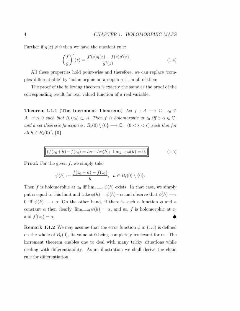
The proof of the following theorem is exactly the same as the proof of the

corresponding result for real valued function of a real variable.

Theorem 1.1.1 (The Increment Theorem:) Let f : A −→ C, z0 ∈A, r > 0 such that Br(z0) ⊂ A. Then f is holomorphic at z0 iff ∃ α ∈ C,

and a set theoretic function φ : Bs(0) \ 0 −→ C, (0 < s < r) such that for

all h ∈ Bs(0) \ 0

(f(z0+h)−f(z0) = hα+hφ(h); limh→0 φ(h) = 0. (1.5)

Proof: For the given f, we simply take

ψ(h) :=f(z0 + h) − f(z0)

h, h ∈ Br(0) \ 0.

Then f is holomorphic at z0 iff limh−→0 ψ(h) exists. In that case, we simply

put α equal to this limit and take φ(h) = ψ(h)−α and observe that φ(h) −→0 iff ψ(h) −→ α. On the other hand, if there is such a function φ and a

constant α then clearly, limh−→0 ψ(h) = α, and so, f is holomorphic at z0

and f ′(z0) = α. ♠

Remark 1.1.2 We may assume that the error function φ in (1.5) is defined

on the whole of Br(0), its value at 0 being completely irrelevant for us. The

increment theorem enables one to deal with many tricky situations while

dealing with differentiability. As an illustration we shall derive the chain

rule for differentiation.

1.1. COMPLEX DIFFERENTIABILITY 5

Theorem 1.1.2 (Chain Rule :) Let f : A −→ C, g : B −→ C, f(A) ⊂B and z0 ∈ A. Suppose that f ′(z0) and g′(f(z0)) exist. Then (g f)′(z0)

exists and (g f)′(z0) = g′(f(z0))f′(z0).

Proof: Let

f(z0 + h) − f(z0) = hf ′(z0) + hη(h); η(h) → 0 as h→ 0;

& g(f(z0) + k) − g(f(z0)) = kg′(f(z0)) + kζ(k) ; ζ(k) → 0 as k → 0

(1.6)

be as in the increment theorem. Let η, ζ be defined over Bs(0), Bs(0) re-

spectively. Since f the continuity of f at z0, it follows that if s is chosen

sufficiently small then for all h ∈ Bs(0), we have f(z0 + h) − f(z0) ∈ Br(0).

Hence we can put k = f(z0 + h) − f(z0), in (1.6) to obtain,

g(f(z0 + h)) − g(f(z0)) = [hf ′(z0) + hη(h)][g′(f(z0)) + ζ(k)]

= hg′(f(z0))f′(z0) + hξ(h),

where, ξ(h) = η(h)g′(f(z0)) + (η(h) + f ′(z0))ζ(f(z0 + h) − f(z0)). Observe

that as h → 0, we have, k = f(z0 + h) − f(z0) → 0 and ζ(k) → 0. Hence

ξ(h) → 0, as h→ 0. Thus by the increment theorem again, (g f)′(z0) exists

and is equal to g′(f(z0))f′(z0) as desired.

Remark 1.1.3 So far, we have considered derivatives of functions at a point

z ∈ A only when the function is defined in a nbd of z. We can try to relax

this condition as follows: Thus, if B ⊂ C and f : B −→ C, we say f is

holomorphic on B if f extends to a holomorphic map f : A −→ C where A

is an open subset containing B. However, we can no longer attach a unique

derivative to f at points of B in general. With some more suitable geometric

assumptions on B, this can be made possible. For instance if B is a closed

disc or a closed rectangle, and if f : B −→ C is differentiable on B, then

even at the boundary points of B, the derivative of f is unique. However,

this is only for curiosity; we shall never have any opportunity to use such

finer treatment in this text.

6 2.4 Polynomials and Rational Functions

sectionPolynomials and Rational Functions

In this section, let us study some simple examples holomorphic functions:

(a) The polynomial functions: As such, the easiest functions to deal

with are the constant functions. These are the first examples of holomorphic

functions. The identity function z 7→ z, merely denoted by z is also holo-

morphic. Let n be a non negative integer. By a polynomial function p(z) of

degree n, we mean a function of the form

p(z) = a0 + a1z + a2z2 + · · · + anz

n,

ai ∈ C, an 6= 0. Since scalar multiples, sums and products of holomorphic

functions are holomorphic, it follows that any polynomial function is holo-

morphic. Moreover, the (Cauchy derivative) complex derivative of p is easily

seen to be given by

p′(z) = a1 + 2a2z + · · ·nanzn−1.

Observe that all constant functions a 6= 0 have degree 0. The ‘zero’ function is

customarily assigned degree −∞, but often it can be assigned any particular

degree depending upon the context. All degree 1 polynomials are also referred

to as linear polynomials. The fundamental theorem of algebra (FTA)

asserts that every non-constant polynomial assumes the value zero, i.e., the

equation

p(z) = 0

has a solution. This is the same as saying every non constant polynomial

has a root. We have already seen a proof of this theorem in chapter 1. Now

observe that if z1 is a solution of p(z) = 0, then as in school algebra, we can

perform division by z − z1 and the remainder will be zero, i.e.,

p(z) = q(z)(z − z1).

Ch. 2 Holomorphic and Analytic Functions 7

It also follows easily that deg q(z) = n− 1. Thus by repeated application of

FTA, we can factorize p(z) completely into linear factors and a constant:

p(z) = an(z − z1)(z − z2) · · · (z − zn), an 6= 0. (1.7)

We conclude that every polynomial of degree n has n roots. Also if

w 6= zi, i = 1, . . . , n, it is clear from (1.7) that p(w) 6= 0. Hence, p(z) has

precisely n roots. Observe that two or more of the roots zj may coincide. If

that is the case, we say, that the corresponding root is a multiple root with

its order or multiplicity being equal to the number of times z−zj is repeated

in the factorization (1.7). The factorization is unique up to a permutation

of the factors.

Next, we observe that if z1 is a repeated root then p′(z1) = 0. Indeed if

the multiplicity of z1 is m in p(z) then

p(z) = (z − z1)mq(z), (q(z1) 6= 0)

which implies that,

p′(z) = m(z − z1)m−1q(z) + (z − z1)

mq′(z) = (z − z1)m−1r(z),

where r(z) = mq(z) + (z − z1)q′(z). Since r(z1) 6= 0, it follows that the

multiplicity of z1 in p′(z) is m− 1.

As an entertaining exercise, let us prove the following theorem due to

Gauss which has a lot of geometric content in it. Recall that if S is a subset

of C, then by convex hull of S we mean the set of all elements∑tjSj where

the sum is finite, 0 ≤ tj ≤ 1 and∑tj = 1.

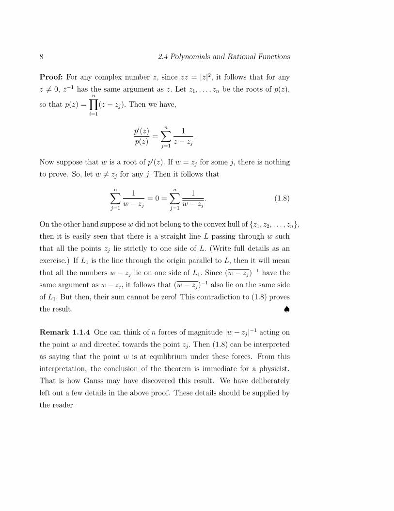
Theorem 1.1.3 Gauss2: Let p(z) be a polynomial with complex coefficients.

Then all roots of p′(z) lie in the convex hull spanned by the roots of p(z).

2An equivalent version of this has been attributed to Lucas by Ahlfors.

8 2.4 Polynomials and Rational Functions

Proof: For any complex number z, since zz = |z|2, it follows that for any

z 6= 0, z−1 has the same argument as z. Let z1, . . . , zn be the roots of p(z),

so that p(z) =n∏

i=1

(z − zj). Then we have,

p′(z)

p(z)=

n∑

j=1

1

z − zj.

Now suppose that w is a root of p′(z). If w = zj for some j, there is nothing

to prove. So, let w 6= zj for any j. Then it follows that

n∑

j=1

1

w − zj

= 0 =n∑

j=1

1

w − zj

. (1.8)

On the other hand suppose w did not belong to the convex hull of z1, z2, . . . , zn,then it is easily seen that there is a straight line L passing through w such

that all the points zj lie strictly to one side of L. (Write full details as an

exercise.) If L1 is the line through the origin parallel to L, then it will mean

that all the numbers w − zj lie on one side of L1. Since (w − zj)−1 have the

same argument as w− zj , it follows that (w − zj)−1 also lie on the same side

of L1. But then, their sum cannot be zero! This contradiction to (1.8) proves

the result. ♠

Remark 1.1.4 One can think of n forces of magnitude |w− zj |−1 acting on

the point w and directed towards the point zj . Then (1.8) can be interpreted

as saying that the point w is at equilibrium under these forces. From this

interpretation, the conclusion of the theorem is immediate for a physicist.

That is how Gauss may have discovered this result. We have deliberately

left out a few details in the above proof. These details should be supplied by

the reader.

Ch. 2 Holomorphic and Analytic Functions 9

(b) The rational functions: In (a), the domain of definition of our func-

tions were not mentioned. However, note that all those functions were defined

throughout C.

We shall now define some holomorphic functions with their domains of

definition not necessarily being the entire plane. These are functions of the

form

φ(z) =p(z)

q(z)(1.9)

where p and q are polynomials, called rational functions. By canceling out

common factors from both p and q, we can assume that p and q do not have

any common factors. Then, obviously, φ(z) makes sense only when q(z) 6= 0

and so the domain of definition of φ(z) is C \ z : q(z) = 0. We have by

1.4,

φ′(z) =p′(z)q(z) − q′(z)p(z)

(q(z))2(1.10)

and so φ is holomorphic in its domain. Its derivative is another rational func-

tion having the same domain of definition. Prove this statement. Caution:

(1.10) may not be in the reduced form even though (1.9) is. Later on, we shall

have more opportunities to study these functions, particularly, the so called

fractional linear transformations, which are of the formaz + b

cz + d. At this stage,

it may be worthwhile to note that the set of all polynomials in one variable

with complex coefficients forms a commutative ring which we denote by C[z].

One of the important property of this ring is that it is an integral domain ],

(i.e., a commutative ring in which product of two non zero elements is never

zero. This follows easily from the ‘unique factorization’ property (1.7) that

we have seen. The set of all rational functions forms a field, C(z), called the

field of fractions of the integral domain C[z].

In order to get any other class of examples of complex differentiable func-

tions, we have to use the power series. This topic will be taken up soon by

10 3.1 Cauchy–Riemann Equations

Prof. K. D. Joshi.

Let us now try to understand the complex differentiability a little more

closely.

1.2 Cauchy–Riemann Equations

Definition 1.2.1 Let U be an open subset of C, z0 = (x0, y0) ∈ U and

f : U −→ C be a given function. By keeping the variable y constant at

y = y0 and varying only x, we obtain a function of one variable out of f.

More precisely, choose ǫ > 0, so that for |t| < ǫ, the points (x0 + t, y0) are

inside U. Let

F (t) = f(x0 + t, y0). (1.11)

Then F is a function of a real variable t. Of course, it may be a complex

valued function though. Nevertheless, we can talk about differentiability of

this function at the point 0. We say the partial derivative of f with respect

to the variable x exists at z0 iff F is differentiable at 0 and in this case we

set F ′(0) to be the partial derivative of f with respect to x. This is denoted

by fx(z0) or∂f

∂x(z0).

Observe that F is nothing but the restriction of f to the line through z0

parallel to the x−axis. Similarly, by taking the function f restricted to line

through z0, parallel to the y−axis, the partial derivative with respect to y is

also defined and denoted by fy or∂f

∂y(z0) .

Write z = x + ıy, z0 = x0 + ıy0, h = h1 + ıh2, f(x + ıy) = u(x, y) +

ıv(x, y). Suppose f ′(z0) exists and let f ′(z0) = α + ıβ. By the increment

theorem, we have

f(z0 + h) − f(z0) = hf ′(z0) + hη(h); η(h) → 0 as h→ 0. (1.12)

Ch. 3 Conformality 11

Put η(h) = η1(h) + ıη2(h), where η1, η2 are real and imaginary parts of η.

Then clearly,

ηj(h) −→ 0 as h −→ 0. (1.13)

Put h = h1 in (1.12), i.e., take h2 = 0, to obtain

f(x0 + h1, y0) − f(x0, y0) = h1(α + ıβ) + h1η(h1). (1.14)

Comparing the real and the imaginary parts on both the sides we get

u(x0 + h1, y0) − u(x0, y0) = h1α+ h1η1(h1);

and v(x0 + h1, y0) − v(x0, y0) = h1β + h1η2(h1).

(1.15)

Therefore, by the increment theorem for 1-variable functions, it follows

that ux and vx exist at (x0, y0) and we have,

ux(x0, y0) = α, vx(x0, y0) = β. (1.16)

Now put h = ıh2, i.e., take h1 = 0 in (1.12), to obtain

f(x0, y0 + h2) − f(x0, y0) = ıh2(α + ıβ) + ıh2η(ıh2)

Again, comparing the real and imaginary parts and using increment theorem,

we obtain

uy(x0, y0) = −β; vy(x0, y0) = α. (1.17)

Thus (1.16) and (1.17) together give

ux(x0, y0) = vy(x0, y0); uy(x0, y0) = −vx(x0, y0) (1.18)

These are called Cauchy–Riemann(CR)-equations.3 Observe that we also

have.

f ′(z0) = ux(x0, y0) + ıvx(x0, y0) (1.19)

= vy(x0, y0) − ıuy(x0, y0) (1.20)

3Bernhard Riemann(1826-1866) a German mathematician.


and

|f ′(z0)|2 = u2x+v2

x = u2y+v2

y = u2x+u2

y = v2x+v2

y = uxvy−uyvx. (1.21)

The last expression above, which is the determinant of the matrix

[ux uy

vx vy

](1.22)

is called the jacobian of the mapping f = (u, v), with respect to the variables

(x, y) and is denoted by

J(x,y)(u, v) := uxvy − uyvx. (1.23)

Remark 1.2.1 A simple minded application of CR-equations is that it helps

us to detect easily when a function is not C-differentiable. For example,

ℜ(z),ℑ(z) etc are not complex differentiable anywhere. The function z 7→|z|2 is not complex differentiable for any point z 6= 0. However, it satisfies the

CR-equations at 0. That of course does not mean that it is C-differentiable

at 0. (See the exercise below.)

In order to understand the full significance of CR-equations, we must

know a little more about calculus of two real variables. In the next section,

we recall some basic results in real multi-variable calculus. and then study

the close relationship between complex differentiation and the real total dif-

ferentiation. You may choose to skip this section and come back to it if

necessary while reading the section after that. However, try all the following

exercises before going further. If you have difficulty in solving any of them,

then perhaps you must read the next section thoroughly.

Exercise 1.2.1

1. Use CR equations to show that z −→ ℜ(z), z −→ ℑ(z) are not

complex differentiable anywhere.

1.3. REVIEW OF CALCULUS OF TWO REAL VARIABLES 13

2. Use polar coordinates to show that z 7→ |z|2 is complex-differentiable

at 0. What about the function z 7→ |z|?.

3. Suppose f is a complex differentiable everywhere on an open disc D and

takes real values only. Then show that f is a constant. [Hint Use CR

equations.] Let now f : D → C be a complex differentiable function.

Suppose its image is contained in a line or a circle or a parabola. Then

prove that f is a constant.

1.3 Review of Calculus of Two Real Variables

We will need some basic notions of the calculus of two real variables. In this

section, we recall these concepts to the extent required to understand the

later material that we are going to learn. Indeed, we presume that you are

already reasonably familiar with the material of this section.

As a warm-up, we illustrate the kind of danger that we may be in while

we are trying to relate the calculus of several variables to that of 1-variable,

with an example.

Example 1.3.1 Define a function f : R2 −→ R by

f(x, y) =

xy

x2 + y2, if (x, y) 6= (0, 0)

0, if (x, y) = (0, 0)(1.24)

This function has questionable behavior only at (0, 0). It has the property

that for each fixed y, it is continuous for all x and for each fixed x it is

continuous for all y. Moreover, if you restrict the function to any line, it is

continuous. However, it is not continuous at (0, 0) even if we are ready to

redefine its value at (0, 0). This is checked by taking limits along the line

y = mx. For different values of m, we get different limits at (0, 0). So, there

is no way we can make it continuous at (0.0).


We begin by recalling the increment theorem of 1-variable calculus.

Theorem 1.3.1 Let f : (a, b) −→ R be a function x0 ∈ (a, b). Then f

is differentiable at x0 iff there exists an error function η defined in some

neighborhood |x− x0| < ǫ of x0 and a real number α such that

f(x0 +h)−f(x0) = αh+η(h)h, and η(h) −→ 0, as h −→ 0. (1.25)

Remark 1.3.1 The proof of this is exactly same as that of theorem 1.1.1.

Roughly speaking, the condition in the increment theorem tells us that the

difference (increment) in the functional value of f at x0 is f ′(x0) times the

difference (increment) h, in the variable x, up to a second order term viz.,

hη(h). That explains why this result is called the increment theorem. It is

also referred to as linear approximation to f and is written in the form

f(x0 + h) ≈ f(x0) + hf ′(x0)

We know that f ′(x0) is the slope of the tangent to the graph of the function

y = f(x). We also know that a line in R2 is the graph of a linear map. Since

the tangent line represents an approximation of the graph of the function f,

we may say that the linear map corresponding to the tangent line represents

an approximation to the function f at x0. Thus we see that the derivative

should be thought of as a linear map approximating the given function at

the given point. This aspect of the differentiability of a 1-variable function is

obscured by the over simplification that occurs naturally in 1-variable linear

algebra viz., ‘a linear map R −→ R is nothing but the multiplication by a

real number and thus can be identified with that real number’. When we pass

to two or more variables, this simplification disappears and thus the true

nature of the derivative comes out, as in the following definition. In what

follows, we restrict our attention to two variables, though there logical gain

in it. All the concepts and results that we are going to introduce for two

variables hold good for more number of variables also.


Definition 1.3.1 Let U be an open subset of R2 and let f : U −→ R be

any function. Let z0 be any point in U. We say f is ((Frechet4) differentiable

at z0 iff there exists a linear map L : R2 −→ R and a scalar valued error

function η defined in a neighborhood of z0 in U such that

f(z0+h)−f(z0) = L(h)+‖h‖η(h); η(h) −→ 0 as h −→ 0. (1.26)

Further L is called the Frechet derivative or the total derivative of f at z0

and is denoted by (Df)z0. If f is differentiable at each point of U then it is

called a (Frechet) differentiable function.

As an easy exercise prove the following theorem:

Theorem 1.3.2 If f is differentiable at a point then it is continuous at that

point.

Theorem 1.3.3 Let U, f, z0 = (x0, y0) etc. be as above. Let f be Frechet

differentiable at z0. The f has its partial derivatives at z0 and moreover we

have

fx(z0) = (Df)z0(1, 0); fy(z0) = (Df)z0

(0, 1).

Proof: Let L = (Df)z0. Putting h = (t, 0) in (1.26), we obtain,

F (t) − F (0) = L(t, 0) + η(t, 0)|t| = tL(1, 0) + η(t, 0)|t|. (1.27)

Dividing out by t and taking limit as t −→ 0, it follows that F ′(0) exists i.e.,

fx(z0) exists and is equal to L(1, 0). Similarly, we can show that fy exists

and fy(z0) = L(0, 1). ♠

Remark 1.3.2

(i) In (1.27), can you rewrite the rhs in form of (1.5)? If so, you don’t have

4Rene Maurice Frechet (1878-1973).


to divide by t and take the limit etc. as in we did in the proof above.

(ii) The concept of partial derivative is a special case of a more general

concept. Given any unit vector u, we define the directional derivative of f in

the direction of u denoted by Duf(z0), to be the limit of

limt−→0

f(z0 + tu) − f(z0)

t

provided it exists. As above, it can be seen that all the directional derivatives

exist if (Df)z0exists. Moreover, by putting h = tu, in (1.26), dividing out

by t and then taking the limit as t −→ 0, it is verified that Duf(z0) =

L(u)(Df)z0· u, where · denotes the dot product.

(iii) It may happen that all the directional derivatives exist and yet the total

derivative (Df)z0may not exist. This can happen even if all this directional

derivatives vanish, as seen in the following two examples.

Example 1.3.2 Consider the function

f(x, y) =

x2y

x4 + y2, (x, y) 6= (0, 0),

0, (x, y) = (0, 0).

Clearly f is differentiable at all points except perhaps at (0, 0). We shall show

that f is not even continuous at (0, 0) and hence cannot be differentiable at

(0, 0). However, observe that if you restrict the function to any of the lines

through the origin, then it is continuous. This will tell you that if we approach

the origin along any of these lines then the limit of the function coincides

with the value of the function. In contrast, in the case of 1-variable function,

if the left-hand and right-hand limits existed and agreed with the functional

value then the function was continuous at that point. Thus, the geometry of

the plane is not merely the geometry of all the lines in it.

In order to see that the function is not continuous at the origin, we

shall produce various sequences un such that limn−→∞ un = (0, 0) and


limf(un) takes different values. It then follows that, at (0, 0), even a

redefinition of f will not make it continuous. So take any real sequence

xn −→ 0, xn 6= 0 and put yn = kx2n for some real k. Put un = (xn, yn). Then

un −→ (0, 0) and f(un) = k/(1+k2). Therefore, limn−→∞ f(un) = k/(1+k2).

Thus for different values of k we get different values of this limit as required.

On the other hand, let u = (a, b) be a unit vector. If b is zero then

clearly the partial derivative of f in the direction of u (it is fx) is zero since

the function is identically zero on the x axis. For b 6= 0, we have Fu(t) =

a2bt/(t2a4 + b2) for all t. It follows that Duf(0, 0) = F ′u(0) = a2b/b2 = a2/b.

Thus all the directional derivatives exist. Also, for your own satisfaction

check that the partial derivatives are not continuous at (0, 0).

Example 1.3.3 We can improve upon the above example 1.3.2, as follows.

Take g(x, y) =√x2 + y2f(x, y), where f is given as in example 1.3.2. Then

the function g is continuous also at (0, 0) and has all the directional deriva-

tives vanish at (0, 0). That means that the graph of this function has the

xy-plane as a plane of tangent lines at the point (0, 0, 0). We are tempted

to award such ‘nice’ geometric behavior of the function and admit it to be

‘differentiable’ at (0, 0). Alas! Even then it is not differentiable at (0, 0), in

the definition that we have adopted. For

g(x, y) − g(0, 0)

‖(x, y)‖ = f(x, y)

has no limit at (0, 0).

We hope that the above two examples illustrate the subtlety of the situ-

ation in the following theorem, which is a result in the positive direction.

Theorem 1.3.4 Let U be an open set in C, and f : U → R be a function

having partial derivatives which are continuous at (x0, y0). Then f is Frechet

differentiable at (x0, y0).


Proof: By Mean Value theorem of 1-variable calculus, there exist 0 ≤ t, s ≤ 1

such that f(x0 + h, y0 + k) − f(x0 + h, y0) = kfy(x0 + h, y0 + sk);

f(x0 + h, y0) − f(x0, y0) = hfx(x0 + th, y0). (Of course t, s depend on h, k.)

Therefore,

|f(x0 + h, y0 + k) − f(x0, y0) − hfx(x0, y0) − kfy(x0, y0)|≤ |h||fx(x0 + th, y0) − fx(x0, y0)| + |k||fy(x0 + h, y0 + sk) − fy(x0, y0)|.By continuity of fx, fy at (x0, y0) given ǫ > 0, we can choose h, k sufficiently

small so that |fx(x0+th, y0)−fx(x0, y0)| < ǫ; |fy(x0+h, y0+sk)−fy(x0, y0)| <ǫ. The conclusion follows. ♠

A slight variation of the above result is given below. The proof is left to

you as a simple exercise.

Theorem 1.3.5 Let U be an open subset of C and f : U −→ R be a func-

tion. Then f is Frechet differentiable at U and the function f ′ : U −→ C is

continuous iff both the partial derivatives of f exist on U and are continuous

on U.

Observe that the assignment x 7→ (Df)x defines a map Df of U into

the space of all linear maps R2 into R viz., the dual vector space R

2⋆ which

is isomorphic to R2. So, one can define f to be continuously differentiable if

Df is defined and continuous. Since the two coordinate functions of Df are

nothing but the two partial derivatives, the continuity of Df is equivalent to

that of the continuity of the two partial derivatives of f.

Of course, if this is true for all points x ∈ U then we say f is continuously

differentiable in U or f is of class C1 in U. Inductively, a function f on U is

said to be of class Cr in U if all the partial derivatives of f of order r exist

and are continuous in U. Finally, a function which is of class Cr for all r > 0

is said to be of class C∞.

Also observe that in the case of one variable, we get back our old definition

provided we identify (Df)z0with L(1).


Remark 1.3.3 All the standard properties of the derivatives of a function

of one variable such as for sums and scalar multiples etc. hold here also

with obvious modifications wherever necessary. For instance, if f and g are

real valued differentiable functions then their product is differentiable and

we have

D(fg)(z0) = f(z0)D(g)(z0) + g(z0)D(f)(z0).

It may be worth recalling that Mean Value Theorem is one result which really

needs modification.

Definition 1.3.2 Let f : U −→ R2 be a function and z0 be a point of

the open set U ⊂ C. We say f is differentiable at z0 there exists a linear

map L : R2 −→ R

2 and an error function η : Br(0) −→ R2 such that for

h ∈ Br(0), we have,

(f(z0 + h) − f(z0) = L(h) + |h|η(h); limh→0 η(h) = 0. (1.28)

In this case, We write D(f)z0= L.

Theorem 1.3.6 Let f : U −→ V and g : V −→ R be such that f is

differentiable at z0 ∈ U and g is differentiable at w0 = f(z0) ∈ V. Then

g f is differentiable at z0 and we have,

D(g f)z0= D(g)w0

D(f)z0.

Proof: We have

f(z0 + h)− f(z0) = L1(h) + |h|η1(h); g(w0 + k)− g(w0) = L2(k) + |k|η2(k),

where η1(h) −→ 0 as h −→ 0 and η2(k) −→ 0 as k −→ 0. Note that

f(z0 + h) − f(z0) −→ 0 as h −→ 0. Therefore, we can substitute k =

f(z0 + h) − f(z0) in the second equation. This gives,


g f(z0 + h) − g f(z0) = L2(L1(h) + |h|η1(h)) + |h|( ||k||

|h| η2(k)

)

= L2 L1(h) + |h|(L2(η1(h)) +

|k||h|η2(k)

)

Observe that|k||h| ≤

‖L1(h)‖|h| + ‖η1(h)‖ −→ ‖L1‖.

Therefore, if we take η(h) = L2(η1(h)) + |k||h|η2(k), it follows that η(h) −→ 0

as h −→ 0. The result follows. ♠As an easy consequence, we can now derive:

Theorem 1.3.7 Let U be a convex open subset of R2 and f : U −→ R

2 be

a differentiable function such that D(f)z = 0 for all z ∈ U. Then f(z) = c, a

constant, on U.

Proof: Fix a point z0 ∈ U. Now for any point z ∈ U consider the map

g : [0, 1] −→ U given by g(t) = (1−t)z0+tz. By chain rule the composite map

h := f g : [0, 1] −→ is differentiable and its derivative vanishes everywhere.

By 1-variable calculus, (Lagrange’s Mean Value theorem), applied to each

component of h = (h1, h2) it follows that h is a constant function on [0, 1].

In particular, h(1) = h(0). But f(z) = h(1) = h(0) = f(z0). ♠

Remark 1.3.4 Observe that the projection maps are differentiable. There-

fore, it follows that if f = (f1, f2) is differentiable then each co-ordinate

function fj is also so. It is not difficult to see that the converse is also true.

The derivatives D(f1) andD(f2) can be treated as row vectors and by writing

them one below the other, we get a 2 × 2 matrix D(f). With this notation,

the chain rule can be stated in terms of matrix multiplication.

Having identified a linear map L : R2 −→ R

2 with a 2 × 2 real matrix,

we see that D(f) is a function from U to M(2; R). The latter space can

1.4. CAUCHY DERIVATIVE (VS) FRECHET DERIVATIVE 21

be identified with the Euclidean space R4. We can then see that D(f) :

U −→ R4 is continuous iff the partial derivatives of f1, f2 are continuous.

The map f : U −→ R2 is called a map of class C1 on U if it is differentiable

and the derivative D(f) is continuous. (This also goes under the somewhat

loose terminology ‘continuously differentiable’.) What is then the meaning

of D(f) : U −→ R4 is differentiable? Going by the above principle, we

see that this is the same as saying that all the four component functions of

D(f) should be differentiable. The derivative of D(f) is actually a function

D2(f) : U −→ R8. Components of this are nothing but the second order

partial derivatives of the components of f. Thus for any positive integer k,

we define f to be of class Ck on U if all its k-th order partial derivatives exist

and are continuous on U. If f is of class Ck for all k ≥ 1 then it is said to

belong to the class C∞. Such maps are also called smooth maps.

All this can be easily generalized to functions from subsets of Rn to R

m

for any positive integers m,n.

1.4 Cauchy Derivative (Vs) Frechet Deriva-

tive

Partial derivatives play a key role in the comparison study of Cauchy deriva-

tive and Frechet derivative. We have seen that existence of either of them

implies the existence of partial derivatives. Moreover, in the former case, the

partial derivatives satisfy the CR-equations. Thus, even if Df exists, if CR

equations are not satisfied then f ′ does not exist. Using this we can give

plenty of examples of non-holomorphic functions which are Frechet differen-

tiable. As we have already seen, the geometry of the plane is responsible for

making the total derivative somewhat subtler in comparison with the deriva-

tive in the case of one 1-variable function. What additional basic structure


is then responsible for the difference in Cauchy differentiation and Frechet

differentiation? An answer to this question is in the following theorem:

Theorem 1.4.1 Let f : U −→ C be a continuous function, f = u + ıv,

z0 = x0 + ıy0 be a point of U. Then f is C-differentiable at z0 iff considered

as a vector valued function of two real variables, f is (Frechet) differentiable

at z0 and its derivative (Df)z0: C −→ C is a complex linear map. In that

case, we also have f ′(z0) = (Df)z0.

Proof: Recall that a map φ : V −→W of complex vector spaces is complex

linear iff φ(αv + βw) = αφ(v) + βφ(w) for any α ∈ C and v, w ∈ V. Let us

first consider a purely algebraic problem: Treating C as a 2-dimensional real

vector space, consider a real linear map T : C −→ C given by the matrix(a b

c d

)

When is it a complex linear map? We see that, if T is complex linear, then

T (ı) = ıT (1) and hence, b+ ıd = T (ı) = ıT (1) = ı(a+ ıc). Therefore, b = −cand a = d. Conversely, it is easily seen that this condition is enough to ensure

the complex linearity of T.

Coming to the proof of the theorem, suppose that f is C-differentiable at

z0. Then as already seen the partial derivatives exist and satisfy the Cauchy–

Riemann equations. So, the 2×2 matrix (1.22) defines a complex linear map

from C to C. It remains to see that f is real differentiable at z0, for then,

automatically the derivative will be equal to the matrix (1.22) above. For

this, we directly appeal to the increment theorem: We have,

f(z0 + h) − f(z0) = (α + ıβ)h+ hη(h),

where, α = ux = vy, β = vx = −uy. Put φ(h) =h

‖h‖η(h). Then,

limh→0

‖φ(h)‖ = limh→0

‖η(h)‖ = 0.


Also, the multiplication map h 7→ (α + βı)h can be viewed as a real linear

map acting on the 2-vector h, it follows that f is Frechet differentiable, with

the derivative Df given by (1.22).

Conversely, assume that Df exists and is complex linear. The existence

of Df means that there exist error functions ζ and γ say, such that

u(z0 + h) − u(z0) = (h1ux + h2uy) + |h|ζ(h)v(z0 + h) − v(z0) = (h1vx + h2vy) + |h|γ(h)

(1.29)

with ζ(h) −→ 0 and γ(h) −→ 0 as h −→ 0. Complex linearity of Df means

that ux = vy := α say, uy = −vx := β say. Then, multiply the second

equation by ı and add it to the first equation above to obtain

f(z0 + h) − f(z0) = h(α+ ıβ) + |h|(ζ(h) + ıγ(h)),

where,

limh−→0

|h|(ζ(h) + ıγ(h))

h= 0.

Finally, in this case, the complex linear map D(f)z0given by the matrix

(1.22) is nothing but multiplication by the complex number ux+ıuy = f ′(z0).

Hence, the proof of the theorem is complete. ♠As an immediate corollary, we have,

Theorem 1.4.2 Let f : U −→ C be a complex differentiable function in a

convex domain U such that f ′(z) ≡ 0. Then f is a constant on U.

Proof: By the previous theorem the Frechet derivative of f vanishes in U

and so we can apply theorem 1.3.7. ♠

There are certain useful partial results that relate the two notions of

differentiability. We shall mention some of them here without proof. The

most popular one is:


Theorem 1.4.3 Let f be a continuous complex valued function of a complex

variable defined on an open subset U, possessing continuous partial deriva-

tives. Then f is complex differentiable in U iff it satisfies the Cauchy–

Riemann equations in U.

Proof: The only if part has been proved already. The if part is the con-

sequence of theorems 1.3.5 and 1.4.1. along with the observation that CR-

equations are equivalent to say that the Frechet derivative is complex linear.

We can improve upon this by:

Theorem 1.4.4 Let f be a continuous complex valued function of a complex

variable defined on an open subset U. Then f is complex differentiable in U

iff it has continuous partial derivatives in U which satisfy CR equations.

Remark 1.4.1 In the ‘only if’ part, the only thing that is not proved already

is the continuity of the partial derivatives. We shall not prove it here. It will

follow once we show that any Cauchy differentiable function has a continuous

derivative. Indeed, we shall see later on that complex differentiability ensures

that the function has continuous derivatives of all orders!

The next step is to remove even the continuity hypothesis on the partial

derivatives. This has to be done carefully as in the following result known

as Looman-Menchoff Theorem It is the most general result known in

this direction in which the continuity hypothesis on the partial derivatives

is removed. However, observe that this is not a ‘pointwise statement’. The

proof involves ideas that are beyond the theme of this course. Interested

reader can look in [N].

Theorem 1.4.5 Let U be an open subset of C and f : U −→ C be a

continuous function, f = u+ ıv. Suppose the partial derivatives of u, v exist

and satisfy Cauchy-Riemann equations throughout U. Then f is holomorphic

in U.


Remark 1.4.2 There are many functions that are complex differentiable at

a point but not so at any other points in a neighborhood(see the exercises

below). As far as the differentiation theory is concerned such functions are

not of much use to us. We would like to concentrate on those functions which

are differentiable in some non empty open subset of C. Such functions will

be called ‘holomorphic.’ Once again, we emphasize the fact functions which

have first order partial derivatives satisfying C-R equations in a non empty

open subset of C are holomorphic. However, in practice, using C-R equations

to see whether a function is holomorphic or not, would be the last thing that

we would like to do. We should have a large class of holomorphic functions

readily known to us and then often a new one could be expressed in some

nice way in terms of these known ones.

Chapter 2

General Form of Cauchy’s

Theorem

2.1 Homotopy: Simple Connectivity

On a simple open arc, there is ‘essentially’ only one way to go from one point

to another. In contrast, on a circle, there are at least two different ways to

do this. As we have already seen, one can interpret the word ‘to go’ here to

mean ‘to communicate’ or ‘to connect by a path’. Thus the first case could

be referred to as ‘simple connectivity’ and the later as ‘multi-connectivity’.

This is how the originators of this notion must have thought as the words

used by them indicate. In modern times, these notions are made to work in

a larger context and hence a certain abstract, more rigorous and (hence) dry

definitions have been adopted in the study of Algebraic Topology using the

machinery of the fundamental group. We shall not take full recourse to that

here, whereas we shall introduce the concept of homotopy and ‘correct’ mod-

ern definition of simply connectedness. Classically the approach for simply

connectivity came through the properties of integrals on them, and we shall

refer to this by homological simply connectivity.

27

28 CHAPTER 2. GENERAL FORM OF CAUCHY’S THEOREM

Definition 2.1.1 Let ωj : [0, 1] → Ω, j = 0, 1, be any two paths with the

same initial and terminal points:

ω0(0) = ω1(0) = a;ω0(1) = ω1(1) = b.

We say ω0, ω1 are path homotopic to each other in Ω and express this by

writing ω0 ∼ ω1 if there exists a continuous map H : I × I → Ω such that

H(t, j) = ωj(t); H(j, s) = ωj(0), j = 0, 1, 0 ≤ t ≤ 1, 0 ≤ s ≤ 1.

H is called a path-homotopy from ω0 to ω1.

If a = b, that is when both the paths are loops passing through a, the

above path-homotopy gives a ‘loop homotopy’ of loops based at a. If ω0

happens to be the constant loop, we say the loop ω1 is ‘null-homotopic.’

The importance of this notion lies in the following theorem:

Theorem 2.1.1 Homotopy Invariance of Integrals Let f be a holomor-

phic mapping on a domain Ω, and ωj be any two (continuous) contours in Ω

which are path homotopic in Ω. Then∫

ω0

fdz =

∫

ω1

fdz.

Proof: The idea is that the homotopy H defines a ‘continuous family’

ωs : 0 ≤ s ≤ 1 of paths beginning with ω0 and ending with ω1 and

having the same end points. The claim is that for all these paths the integral∫

ωtfdz takes the same value. Unfortunately, even to make sense out of this

claim there is a technical snag: the intermediary paths ωs, 0 < s > 1 may

not be piecewise smooth. Let us agree for a moment that we can handle this,

not so serious a sang.

By compactness, by choosing t, s very close, we can make the entire paths

ωt, ωs to be very close to each other. Fix two such t and s and denote by

2.1. HOMOTOPY: SIMPLE CONNECTIVITY 29

µ = ωt, ν = ωs. We can then cover both of them by a finite number of

discs D1, D2, . . . , Dn such that these discs form a chain viz., Di ∩Di+1 6= ∅.We can then choose a sequence of points a = a0, . . . , an = b; on µ and

a = b0, . . . , bn = b on ν so that ai, bi ∈ Di ∩Di+1. Let µi denote the portion

of the contour µ from ai to ai+1. Similarly define νi also. For any two points

z, w ∈ C, let [z, w] denote the line segment traced from z to w. Let Pi denote

the closed contour [ai, bi] ⋆ νij ⋆ [bi+1, ai+1]. Then for each i the entire closed

contour Pi ⋆ µ−1i lies inside the disc Di and hence by Cauchy’s theorem, the

integral of f along this contour vanishes. Therefore∫

µi

fdz =

∫

Pi

fdz, i = 0, 1, . . . , n− 1. (2.1)

Therefore

∫

µ

fdz =n−1∑

i=0

∫

µi

fdz =n−1∑

i=0

∫

Pi

fdz =

∫

ν

fdz, (2.2)

the last equality follows since a0 = b0 = a, an = bn = b and the integrals over

νi occur in pairs in the opposite direction and hence cancel away.

To complete the proof, we have to only say that, by compactness of [0, 1],

there are finitely many points 0 = t1 < · · · < tk = 1 such that any two

consecutive paths ωi := ωti are ‘very close’ to each other.

So, one can ask: can one modify H so that ωt are all piecewise smooth?

The general answer is ‘yes’ but then we are getting into deeper trouble.

Instead, we see a short cut here.

We carry out every thing as described above except the steps (2.1) and

(2.2), which may not make sense because the intermediary the intermediary

paths ωi may not be piecewise smooth. So, we abandon them and replace

them by line segments joining their endpoints, so each Pi is now a piecewise

smooth contour and hence (2.1), (2.2 are valid. ♠

Corollary 2.1.1 Let γ be a null-homotopic contour in Ω. Then for every


holomorphic function f on Ω, we have∫

γ

fdz = 0.

Definition 2.1.2 Let Ω ⊂ C be a domain. We say Ω is simply connected,

if every closed contour in Ω is null-homotopic in Ω.

Remark 2.1.1 The entire plane is simply connected. Indeed any convex

domain in C is simply connected. Simply connectedness is a topological

invariant property, i.e., if X and Y are two spaces which are homeomorphic

to each other then one of them is simply connected iff other is. Thus any

domain which is homeomorphic to a convex domain is simply connected.

At this stage we do not know any other way to see more examples of simply

connected domains. Neither we have any tools to test whether a given domain

is simply connected or not. The above corollary fills this gap to certain extent.

Let restate it as:

Theorem 2.1.2 Cauchy’s Theorem: Homotopy Version Let Ω be a

simply connected domain. Then for every closed contour γ in Ω and every

holomorphic function f,∫

γfdz = 0.

Remark 2.1.2 Thus, if we find one holomorphic function f on Ω and one

closed contour in Ω such that∫

ωf(z)dz 6= 0, then we know that Ω is not

simply connected. Thus C \ 0 is not simply connected because 1/z is

holomorphic on it and its integral on the unit circle is 2πı. Indeed, with this

method, we are sure that given any domain Ω and a finite subset A, the

domain Ω \ A is not simply connected.

We still do not know any method to prove that given Ω is simply con-

nected, when we fail to find such a function and a closed contour.

Theorem 2.1.3 Let Ω be a domain in C. Consider the following statements:

(i) Ω is simply connected.

2.1. HOMOTOPY: SIMPLE CONNECTIVITY 31

(ii) For every closed contour γ in Ω and every holomorphic function f,∫

γfdz = 0.

(iii) Every holomorphic function in Ω has a primitive.

(iv) Every holomorphic function on Ω which never vanishes on Ω has a holo-

morphic logarithm, i.e., there exists a holomorphic function g : Ω → C such

that exp(g(z) = f(z), z ∈ Ω.

(v) For every point a ∈ C \ Ω, and every closed contour γ in Ω, we have,∫

γdz

z−a= 0.

We have (i) =⇒ (ii) =⇒ (iii) =⇒ (iv) =⇒ (v).

Proof: (i) =⇒ (ii) This is the statement of 2.1.2.

(ii) =⇒ (iii) This is the statement of the primitive existence theorem for

each fixed holomorphic function f.

(iii) =⇒ (iv) Apply (ii) to h = f ′/f to obtain g such that g′ = f ′/f. Then

(exp(−g)f)′ = −exp(−g)g′f + exp(−g)f ′ = exp(−g)(−f ′ + f ′) = 0.

Therefore kExp(g) = f for some constant k 6= 0. By choosing g such that

exp(g) and f coincide at a point, we get exp(g) = f.

(iv) =⇒ (v) is obvious. ♠

Remark 2.1.3 Indeed it is true that all these statements are equivalent.

Obviously the difficulty is in proving (v) =⇒ (i) or for that matter in proving

(ii) =⇒ (i). We shall not be able to do this in this chapter. On the other

hand, we shall now launch a programme which will enable us to prove (v) =⇒(ii). On the way, we shall also learn a lot of other related things. Classically,

and in many books even today, simply connectivity is defined by condition

(v). Then the statement ‘(v) implies (ii)’ is known as Homology form of

Cauchy’s theorem. The property (v) can be termed as ‘homological simple

connectivity’ as compared to homotopical one above.


Thus the integral occurring in (v) assumes a special role. We shall take up

the study of this quantity in some detail in the next section, before turning

our attention to actual proof of homology form of Cauchy’s theorem.

2.2 Winding Number

Lemma 2.2.1 Let γ be a closed contour not passing through a given point

z0. Then the integral ω =

∫

γ

dz

z − z0is an integer multiple of 2πi.

Proof: Enough to prove that eω = 1. Define

α(t) :=

∫ t

a

γ′(s)

γ(s) − z0ds; g(t) = e−α(t)(γ(t) − z0); a ≤ t ≤ b.

Since γ is continuous and differentiable except at finitely many points, so is

g. Moreover, wherever g is differentiable, we have

g′(t) = −e−α(t)α′(t)(γ(t) − z0) + e−α(t)γ′(t)

= e−α(t)(−γ′(t) + γ′(t)) = 0.

Therefore, g(t) = g(a) = γ(a) − z0, for all t ∈ [a, b] and hence,

eα(t) =γ(t) − z0γ(a) − z0

,

for all t ∈ [a, b]. Since γ(a) = γ(b), it now follows that eω = eα(b) = eα(a) = 1.

♠

Definition 2.2.1 Let ω be a closed contour not passing through a point z0.

Put ∫

ω

dz

z − z0= 2πım.

Then the number m is called the winding number of the closed contour ω

around the point z0 and is denoted by η(ω, z0). Thus

η(ω, z0) :=1

2πı

∫

ω

dz

z − z0.

2.2. WINDING NUMBER 33

Remark 2.2.1 In order to understand the concept of winding number let

us examine it a little closely.

1. Take z0 = 0 and ω to be any circle around 0. Then we have seen that

∫

ω

dz

z= 2πı.

In other words, η(ω, 0) = 1. So we can say that ω winds around 0

exactly once and this coincides with our geometric intuition.

2. Now let ω be any simple closed contour contained in the interior of an

open disc in the upper half plane. Since 1/z is holomorphic in that disc,

it follows that

∫

ω

dz

z= 0. That means η(ω, 0) = 0. Hence in this case,

we see that the winding number is zero which again conforms with our

geometric understanding.

3. More generally, if ω is contained in a disc, then for all points z outside

this disc, we have η(ω, z) = 0. This is a simple consequence of Cauchy’s

theorem for discs or by simply observing that 1z−a

has a primitive on

the disc. Once again this conforms with our general understanding that

such a contour does not go around z.

4. Let us now consider the curve ω(t) = e2πınt, defined on the interval

[0, 1] for some integer n. This curve traces the unit circle n−times in

the counter clockwise direction. This tallies with the computation of

∫

ω

dz

z= 2πın.

5. It is obvious that η(ω, z) = −η((ω)−1, z). Moreover, if ω = ω1.ω2, then

η(ω, z) = η(ω1, z) + η(ω2, z).


6. By continuity of the integrated function, it follows that z 7→ η(ω, z) is

a continuous function on C \ Im(ω). Being an integer valued continu-

ous function, it must be locally constant. Therefore, it is a constant

function on each path connected subset of C \ Im(ω).

7. Enclosing ω in a large circle C and taking a point z0 outside C, it

follows from (3) that η(ω, z0) = 0. Hence, it follows that η(ω, z) = 0

for all points z in the unbounded component of C \ Im(ω). (Moreover,

any unbounded component should intersect C \ Br(0) for large r and

hence there is only one unbounded component of C \ ω.

Theorem 2.2.1 Cauchy’s Integral Formula ( over simply connected domains):

Let Ω be a simply connected domain on which f is holomorphic. Then for

any point z ∈ Ω and any closed contour ω in Ω not passing through z0, we

have

η(ω; z0)f(z0) =1

2πı

∫

ω

f(z)

z − z0dz. (2.3)

Proof: Consider the function

F (z) =f(z) − f(z0)

z − z0

which holomorphic throughout Ωz0 and has a removable singularity at z0.

Therefore

0 =

∫

ω

F (z)dz =

∫

ω

f(z)

z − z0− 2πıη(ω, z0).

this completes the proof. ♠

Remark 2.2.2 The following special case of theorem 2.2.1 is of utmost im-

portance: Assume that for some component D1 of C \ Im(ω), we have,

η(ω,w) = 1, ∀ w ∈ D1. Then on D1, f itself is represented by

f(w) =1

2πı

∫

ω

f(z) dz

z − w, ∀ w ∈ D1. (2.4)


In particular, the holomorphic function f is completely determined on this

region by the value of f on ω and we have

f(z) =1

2π

∫

ω

f(ξ

ξ − zdξ. (2.5)

D

γ

Ω

1

Fig. 1

Example 2.2.1 Let us find the value of

∫

|z|=1

eaz

zdz.

Observe that eaz is holomorphic on the entire plane C and the curve ω defining

the unit circle has the property η(ω, 0) = 1. Hence, by (2.4), the given integral

is equal to 2πıe0 = 2πı.

Example 2.2.2 As a simple minded application of theorem 2.2.1, let us

prove the non existence of certain roots. Assume that D is a domain which

contains a closed contour ω : [a, b] −→ C, such that η(ω, 0) is odd. Then

we claim that there does not exist any holomorphic function g : D −→


C such that g2(z) = z, z ∈ D. Let us assume on the contrary. Then by

differentiating, we get, 2g(z)g′(z) = 1, z ∈ D. Now,

η(gω, 0) =1

2πı

∫

gω

dw

w=

1

2πı

∫ b

a

g′(ω(t))ω′(t)

g(ω(t))dt =

1

4πı

∫ b

a

ω′(t)

ω(t)dt =

η(ω, 0)

2.

This means that η(ω, 0) is even which is absurd. Similar statements will be

true for other roots also, viz, we do not have a well defined nth root of z− z0

in any domain that contains a closed contour ω such that η(ω, z0) is not

divisible by n.

Example 2.2.3 Let us now consider the function f(z) = 1 − z2 and study

the question when and where there is a holomorphic single valued branch g of

the square root of f i.e., g2 = f. Observe that z = ±1 are the zeros of f and

hence if these points are included in the region then there would be trouble:

By differentiating the identity g2 = f we obtain 2g(z)g′(z) = f ′(z) = −2z.

This is impossible since, at z = ±1, the L.H.S.= 0 and R.H.S. = ∓2. So the

region on which we expect to find g should not contain ±1.

Next assume that Ω contains a small circle C around 1, say, contained in

a punctured disc ∆′ := Bǫ(1)\1 around 1. Restricting our attention to ∆′,

observe that there is a holomorphic branch of the square root of 1 + z say h

defined all over Bǫ(1). Clearly h(z) 6= 0 here and hence φ = g/h will then be

a holomorphic function on ∆′ ∩Ω such that φ2 = 1− z. This contradicts our

observation in the example 2.2.2.

By symmetry, we conclude that Ω cannot contain any circle which encloses

only one of the points −1, 1.

Finally, suppose that both ±1 are in the same connected component of

C \ Ω. Then for all cycles ω in Ω, both ±1 will be in the same connected

component of C \ im ω and hence η(ω, 1) = η(ω,−1). For instance, take

Ω = C\ [−1, 1]. Then for any circle C with center 0 and radius > 1, η(C, 1) =

η(C,−1) = 1.


We shall now see that the square root of f exists. Consider the flt T (z) =1 − z

1 + z. This maps C \ [−1, 1] onto C \ x ∈ R : x ≤ 0, on which we can

choose a well defined branch of the square root function. This amounts to

say that we have a holomorphic function h : C \ [−1, 1] −→ C such that

h(z)2 =1 − z

1 + z. Now consider g(z) = h(z)(1 + z). Then g(z)2 = f(z), as

required.

In fact, Ω(= C \ [−1, 1]) happens to be a maximal region on which 1− z2

has a well defined square root. This follows from our earlier observation that

any such region on which g exists cannot contain a circle which encloses only

one of the two points −1, 1.

Finally, observe that, in place of [−1, 1], if we had any arc joining −1

and 1, the image of such an arc under T would be an arc from 0 to ∞ and

hence on the complement of it, square-root would still exist. Also, the above

discussion holds verbatim to the function (z − a)(z − b) for any a 6= b ∈ C.

You can also modify this argument to construct other roots.

Here is a question then :

Ex. Prove or disprove that f(z) = 1−z2 does not have a well defined

logarithm in C \ [−1, 1].

Definition 2.2.2 Let Ω be a domain ω be a closed contour in it. We say

ω is null homologous in Ω if for every point a ∈ C \ Ω, the winding number

vanishes, η(ω, a) = 0. If every closed contour in Ω is null-homologous in Ω,

we say Ω is homologically simply connected. Two closed contours ω1, ω2 in Ω

are homologous in Ω if η(ω1, a) = η(ω2, a) for all a ∈ C \ Ω.

Theorem 2.2.2 If ω is null-homotopic in Ω then it is null homologous in

Ω. If two contours are path homotopic in Ω then they are homologous in Ω.

A simply connected domain Ω is homologically simply connected.

Proof: This is a direct consequence of theorem 2.1.1.


Remark 2.2.3 In view of (2.2.1.2.2.2), we shall give a sufficient condition

for a contour to have winding number ±1 around a point. This condition is

quite a practical one in the sense that it is easy to verify in many concrete

situations. In the statement of the lemma below, we have simply assumed

that z0 = 0. Of course, this does not diminish the generality of the result, as

we can always perform a translation and choose the origin to be any given

point. The result is important from application as well as theoretical point

of view. However, you may skip learning the proof of this for the time being

and come to it later.

1

2

C C12 0

z

z

ωω21

Lξ

ξ 1

2

Fig. 2

Lemma 2.2.2 Let ω be a contour not passing through 0. Let z1, z2 be two

distinct points on ω and let L be a directed line through 0 so that w1 and

w2 are on the opposite sides of L. Denote the portion of the curve ω from

z1 to z2 in the counter clockwise direction by ω1 and the rest of the portion


by ω2 so that we have ω = ω1.ω2. Assume further that ω1 does not meet the

negative ray of L and ω2 does not meet the positive ray of L. Then

1

2πı

∫

ω

dz

z= η(ω, 0) = ±1.

Proof: Let C be a circle around 0, not meeting ω and let ξ1, ξ2 be the points

on C lying on the line segments [0, z1] and [0, z2] respectively. If C1 and C2

are the portion of the circle traced counter clockwise from ξ1 to ξ2 and from

ξ2 to ξ1 respectively, it follows that C1 does not meet the negative ray of L

and C2 does not meet the positive ray of L. Let

τ1 = [ξ1, z1].ω1.[z2, ξ2].(C1)−1; τ2 = (C2)

−1.[ξ2, z2].ω2.[z1, ξ1].

Then it follows that τi are closed contours and

η(τ1, 0) + η(τ2, 0) = −η(C, 0) + η(ω, 0).

On the other hand, since τ1 does not meet the negative ray of L it follows

that 0 is in the unbounded component of C\Im(τ1) and hence as observed in

remark 2.2.1.7, this implies that η(τ1, 0) = 0. For similar reason η(τ2, 0) = 0.

Therefore,

η(ω, 0) = η(C, 0) = 1.

If we had taken the other orientation on ω, we would have got η(ω, 0) = −1.

This completes the proof of the lemma. ♠As an immediate application we have:

Theorem 2.2.3 Let Ω ⊂ C be a bounded convex region with a smooth bound-

ary C oriented counter clockwise. Then

η(C; a) =

1 a ∈ Ω

0, a ∈ C \ Ω.

In particular, this is true for any disc and any rectangle.


Proof: First consider a ∈ Ω. Any line L through a, cuts C into two parts.

Now for any two points z1, z2 on C lying on opposite sides of L, the hypothesis

of the above lemma is easily verified. This gives the first part.

Now appeal to the fact that C \ C has two components, one of which is

Ω and the other is C \ Ω which is unbounded. By remark 2.2.1.7, the second

part follows. ♠

2.3 Homology Form of Cauchy’s Theorem

Recall that while defining line integrals we first considered differentiable

paths. Then, using the additivity property of the integral so obtained under

subdivision of arcs, we could immediately generalize the definition of the in-

tegral over contours ( which are, by definition, piecewise differentiable paths).

We can now go one step further and allow our contours to have finitely many

discontinuities also. (After all, recall that finitely many jump discontinuities

do not cause any problem in the Riemann integration theory.) But then this

is nothing but merely taking a finite number of contours γi together. Guided

by the property that the integral over two non overlapping contours is the

sum of the integrals over the two contours individually, and by the property

that the integral over the inverse path is the negative of the integral, we now

introduce a formal definition:

Definition 2.3.1 By a ‘chain’ we shall mean a finite formal sum∑

j njγj

where nj are any integers, and γj are contours. In this sum if each γj is a

closed contour, then we call it a cycle. Observe that it does not hurt us if

some of the integers nj are zero. However, we do not generally write such

terms in the summation. We can add two chains and rewrite the sum by

‘collecting terms’ if there are same contours occurring in the summation.

The support of a chain is the set of all image points of all those γj for which

nj is not zero.

2.3. HOMOLOGY FORM OF CAUCHY’S THEOREM 41

The following lemma is central in the proof of Cauchy’s theorem. Pri-

marily, instead of asserting that the formula holds for all contours it says

there is a special one for which it holds. Even though we could do with a

little weaker version of this lemma, we have chosen this form of the lemma,

which can be used for other purposes later. It has its own importance having

a certain topological content.

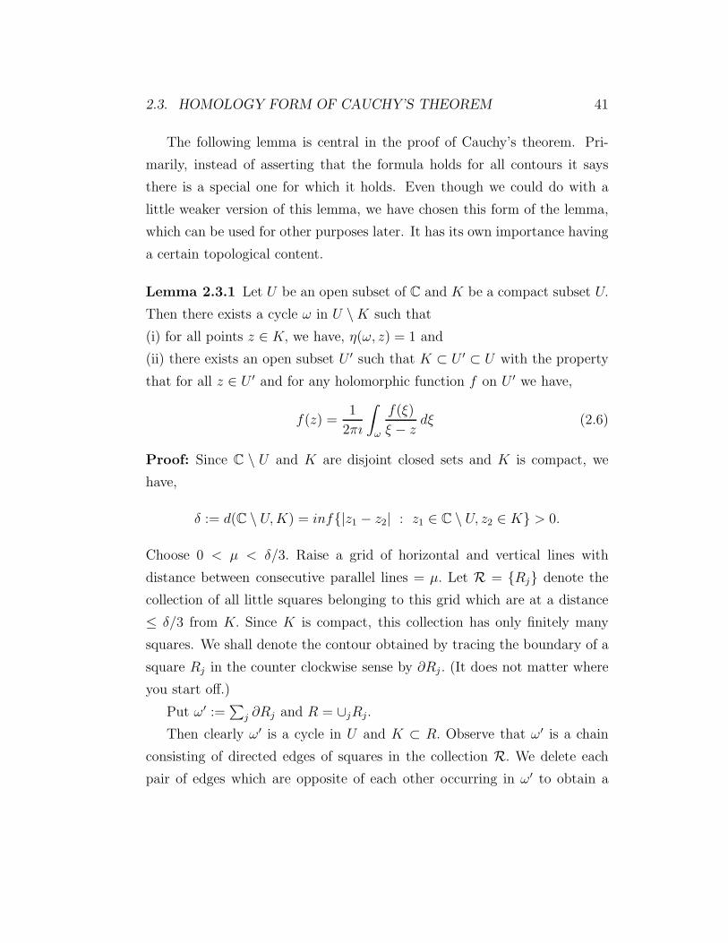
Lemma 2.3.1 Let U be an open subset of C and K be a compact subset U.

Then there exists a cycle ω in U \K such that

(i) for all points z ∈ K, we have, η(ω, z) = 1 and

(ii) there exists an open subset U ′ such that K ⊂ U ′ ⊂ U with the property

that for all z ∈ U ′ and for any holomorphic function f on U ′ we have,

f(z) =1

2πı

∫

ω

f(ξ)

ξ − zdξ (2.6)

Proof: Since C \ U and K are disjoint closed sets and K is compact, we

have,

δ := d(C \ U,K) = inf|z1 − z2| : z1 ∈ C \ U, z2 ∈ K > 0.

Choose 0 < µ < δ/3. Raise a grid of horizontal and vertical lines with

distance between consecutive parallel lines = µ. Let R = Rj denote the

collection of all little squares belonging to this grid which are at a distance

≤ δ/3 from K. Since K is compact, this collection has only finitely many

squares. We shall denote the contour obtained by tracing the boundary of a

square Rj in the counter clockwise sense by ∂Rj . (It does not matter where

you start off.)

Put ω′ :=∑

j ∂Rj and R = ∪jRj.

Then clearly ω′ is a cycle in U and K ⊂ R. Observe that ω′ is a chain

consisting of directed edges of squares in the collection R. We delete each

pair of edges which are opposite of each other occurring in ω′ to obtain a


cycle ω. Clearly, ω is a cycle in U. Integrals over either of these cycles will be

the same for all functions. (In particular the two cycles are homologous to

each other.) Moreover, the support of ω does not intersect K at all. For, if

any edge intersects K, then both the squares of the grid at this edge are in

the collection R and hence, the edge will occur twice, once in each direction,

so gets deleted. This also shows that K is contained in the interior of R,

which we set equal to U ′.

U

U

X

γ

Fig. 4

Now, given any point z in K, since z does not lie on the support of ω, it

follows that η(ω, z) makes sense. Also, every point of K belongs to one of

the squares in R. If z ∈ intRk, then clearly η(∂Rj), z) = 1 if j = k and = 0

otherwise. (See theorem 2.2.3). Therefore, η(ω, z) = η(ω′, z) = 1. Now the

set ∪kintRk is a dense open subset of U ′. We know that winding number is

locally a constant function. It follows that η(ω, z) = 1, for all z ∈ U ′.

2.3. HOMOLOGY FORM OF CAUCHY’S THEOREM 43

To see the second part, let z be in the interior of one of the Rj , s. Then

1

2πı

∫

∂Rk

f(ξ

ξ − zdξ =

f(z) if k = j

0 if k 6= j

Therefore,

f(z) =1

2πı

∫

ω′

f(ξ

ξ − zdξ

for all points in ∪kintRk which is a dense subset of U ′. Since both sides of

the above equation are continuous functions of z on U ′, the validity of the

equation (2.6) for all points of U ′ follows. ♠We are now ready to prove the equivalence of (ii) and (v) of Theorem

2.1.3.

Theorem 2.3.1 Cauchy’s Theorem: Homology Version: Let Ω be a

region in C and γ be a cycle in Ω. Then the following conditions on γ are

equivalent:

(i)

∫

γ

fdz = 0 for all holomorphic functions f on Ω.

(ii) η(γ, a) = 0, for all a ∈ C \ Ω.

Proof: Suppose (i) holds. For any point a ∈ C \ Ω, the function1

z − ais

holomorphic on Ω and hence from (i), we obtain

η(γ, a) =1

2πı

∫

γ

dz

z − a= 0.

This proves the statement: (i)=⇒ (ii).

To prove (ii) =⇒ (i), let A be the unbounded component of C \ supp γand K = C \ A. Since A is open K is closed. Indeed K is the union of all

bounded components and supp γ and hence is bounded. So it is compact.

Take U = Ω ∪K. Then U is open being the union of Ω and all the bounded

components of C\supp γ. By the second part of the lemma 2.3.1, there exists


an open subset U ′ ⊂ U which contains supp γ and a cycle ω disjoint from K

such that for all points z ∈ U ′, we have,

f(z) =1

2πı

∫

ω

f(ξ)dξ

ξ − z.

On the other hand, supp ω ∩K = ∅ =⇒ supp ω ⊂ A =⇒ η(γ, ξ) = 0 for all

ξ ∈ supp ω.

Therefore,

∫

γ

f(z) dz =

∫

γ

(1

2πı

∫

ω

f(ξ)

ξ − zdξ

)dz

=

∫

ω

(1

2πı

∫

γ

dz

ξ − z

)f(ξ) dξ =

∫

ω

η(γ, ξ)f(ξ) dξ = 0

This completes the proof of the theorem. ♠

Chapter 3

Convergence in Function

Theory

3.1 Sequences of Holomorphic Functions

One of the most important results in the theory of convergence of functions

is the majorant criterion of Weierstrass

Theorem 3.1.1 Weierstrass’s Majorant Criterion: Given a series of

functions∑

n fn, suppose there is a convergent series∑

nMn of positive terms

such that |fn(x)| ≤ Mn for all x ∈ X and for all n >> 0, then the series∑

n fn is absolutely and uniformly convergent in X.

Following this, we make some formal definitions: Let fn : X −→ C, n ≥ 1

be a sequence of functions.

Definition 3.1.1 We say the series∑

n fn is compactly convergent in X if

restricted to any compact subset of X, it is uniformly convergent.

Definition 3.1.2 The series∑fn is said to be normally convergent in X if

for every point x ∈ X, there exists a neighborhood U such that∑

n |fn|U <

∞.

45

46 CHAPTER 3. CONVERGENCE IN FUNCTION THEORY

Recall that for each n, |fn|U = sup|fn(z)| : z ∈ U. Observe how Weier-

strass’s criterion has been adopted into a definition here: for a normally con-

vergent series, the terms |fn| play the role of majorants, in the neighborhood

U. It follows that every normally convergent series is locally uniformly conver-

gent inX. Indeed, for series of continuous functions over domains in euclidean

spaces(local compactness!), normal convergence is a convenient terminology

for absolute local uniform convergence. In general, i.e., without continuity of

functions (or local compactness of domains), normal convergence is slightly

stronger than absolutely locally uniform convergence. When each fn is con-

tinuous, it follows that the sum∑fn is also continuous. Linear combination

of normally convergent series is normally convergent. Also the same is true

of Cauchy products of normally convergent series. In addition, because of

the built-in absolute convergence, we have the following two results.

Theorem 3.1.2 Every subseries of a normally convergent series is normally

convergent.

Theorem 3.1.3 Rearrangement Theorem: Let∑fn be a normally con-

vergent series. Then for any bijection τ : N −→ N the series∑fτ(n) is also

normally convergent to the same sum.

Proof: Let f be the sum∑fn. Let x ∈ X and U be a neighborhood of x such

that∑ |fn|U < ∞. By the rearrangement theorem for absolute convergent

series of complex or ( real ) numbers, it follows that∑ |fτ(n)|U is convergent

to∑

n |fn|U . This means that∑fτ(n) is normally convergent. ♠

The following theorem, due to Weierstrass guarantees the holomorphicity

of the limit under normal convergence. It also provides us the validity of

term-by-term differentiation.

Theorem 3.1.4 Weierstrass’ Convergence Theorem: Suppose that we

are given a sequence fn of compactly convergent holomorphic functions in a

3.1. SEQUENCES OF HOLOMORPHIC FUNCTIONS 47

domain D. Then the limit function f is holomorphic and the sequence f(k)n

compactly converges to f (k) on D for every positive integer k.

Proof: Observe that the limit function f is continuous in D due to uniform

convergence on compact sets. Let γ be the boundary of a rectangle contained

in D. Then the sequence fn converges uniformly to f on γ. Hence it follows

that

limn

(

∫

γ

fn(z)dz) =

∫

γ

f(z)dz.

By Cauchy-Goursat theorem, each term on the lhs vanishes and hence rhs

also vanishes. Hence, by Morera’s theorem, it follows that f is holomorphic

at z0 ∈ D.

For the second part, to each closed ball L = B2r(z0) contained D, put

K = Br(z0). First, we use Cauchy’s integral formula to find Mr such that

|f (k)n − f (k)|K ≤Mr|fn − f |L for all n, as follows:

|f (k)n (z) − f (k)(z)| =

∣∣∣∣k!

2πı

∫

C

fn(ξ) − f(ξ)

(ξ − z)k+1dξ

∣∣∣∣

for all z ∈ K. So, we take Mr = k!/rk. Since fn uniformly converges to f on

L, it follows that so does f(k)n to f (k) on K. ♠

Example 3.1.1 As a typical example consider the series

∞∑

n=1

1

nz. If ℜ(z) >

1 + ǫ, then |nz| = n|z| > n1+ǫ and hence the series

∞∑

1

1

n1+ǫis a majorant

for the given series. This implies that∞∑

n=1

1

nzis a normally convergent series

and hence defines a holomorphic function ζ(z) =∞∑

n=1

1

nzin the right-half

plane G1 = z : ℜ(z) > 1. In fact, it is uniformly convergent in G1+ǫ =

x+ ıy : x > 1 + ǫ. This function is called Riemann’s zeta-function.

48 CHAPTER 3. CONVERGENCE IN FUNCTION THEORY

Remark 3.1.1 In the above theorem, one can start with a series which is

normally convergent in D and then conclude similarly with normal conver-

gence of the derived series. However, you may have learnt that a statement

similar to that of the above theorem in the real case is false. A typical counter

example is

fn(x) =x

1 + nx2

defined on the interval (−1, 1). It is not difficult to show that fn compactly

converges to the function f which is identically zero on the interval. But,

0 = f ′(0) 6= limn→∞ f ′n(0) = 1. (Why then does the sequence fn(z) =

z

1 + nz2

not provide a counter example to the above theorem?)

Theorem 3.1.5 Weierstrass’ Double Series Theorem. Consider a se-

quence fm(z) =∑

n amnzn of convergent series in a disc B. Suppose the

series f(z) =∑fm(z) converges normally in B. Then for each n the se-

ries bn =∑

m amn is convergent and f is represented in B by the convergent

power series f(z) =∑

n bnzn.

Proof: Clearly, by the above theorem, f is holomorphic in B. Also f (n) =∑

m f(n)m for all n. Moreover f is represented by the Taylor’s series, f(z) =

∑n f

(n)(0)zn/n!. By substituting expressions for f (n)(0), we obtain the result.

♠

Remark 3.1.2 As an illustration that the Cauchy product of two compactly

convergent series need not be convergent, consider for each n, fn = gn =

(−1)n/√n+ 1, the constant function for all n. Clearly

∑n fn =

∑n gn are

convergent. But the modulus of the kth term of the Cauchy product satisfies:

|hk| =

k∑

m=0

[(m+ 1)(k −m+ 1)]−1/2 >

k∑

m=0

1

k + 1= 1.

Hence the Cauchy product,∑hk is not convergent.

3.1. SEQUENCES OF HOLOMORPHIC FUNCTIONS 49

We shall end this section with a celebrated result due to Hurwitz1 con-

cerning preservation of the zeros under compact convergence.

Theorem 3.1.6 Hurwitz: Let fn be a sequence of holomorphic functions

compactly convergent to f in a region D. If fn have no zeros in D then either

f ≡ 0 or f has no zeros in D.

Proof: Assuming that f 6≡ 0, since the zeros of f are isolated, given

z0 ∈ D, we can choose r > 0 such that A := z : 0 < |z−z0| < r ⊂ D, and

f(z) is holomorphic and not equal to zero on A. If C is the outer boundary of

A, then 1/fn(z) converges uniformly to 1/f(z) on C and since f ′n(z) converges

uniformly to f ′(z) on C, it follows that f ′n(z)/fn(z) converges uniformly to

f ′(z)/f(z) on C. Hence, we have,

∫

C

f ′(z)

f(z)dz = lim

n

∫

C

f ′n(z)

fn(z)dz.

Since fn have no zeros in D every term on rhs is zero. On the other hand,

the lhs counts the number zeros of f inside C. Hence in particular, it follows

that f(z0) 6= 0. ♠

Corollary 3.1.1 In the situation of the above theorem, assume further that

fn is injective in D for all n sufficiently large. Then the limit function f is

either a constant or injective.

Proof: Exercise.

For sharper results in this direction see the excellent book of Remmert p.

261-262.

1Adolf Hurwitz from Zurich is known for his work on analytic functions and Cantor’s

set theory. He should not be confused with V. Hurwitz, who is the author of a famous

book on dimension theory jointly with Wallman.

50 8.2 meromorphic Functions

3.2 Convergence for Meromorphic Functions:

Let us first recall a definition.

Definition 3.2.1 A function f is called meromorphic in a domain D if there

is a closed discrete subset P (f) of D such that f is holomorphic in D \P (f)

and has poles at each point of P (f). Naturally the set P (f) is called the

pole-set of f.

It follows that P (f) is always countable, since every discrete subset of

C is. Observe that, in the definition of a meromorphic function f, we allow

the set P (f) to be empty and thus all holomorphic functions on D are also

meromorphic. Since we know that a meromorphic function tends to ∞ at its

poles, we can think of them as continuous functions on D with values in the

extended complex plane C := C∪∞ by mapping each pole onto ∞. Recall

that if z = z0 is a pole of f of order n ≥ 1, then it is a pole of order n+1 for

f ′. Thus if f is meromorphic, so is f ′ and P (f) = P (f ′). Let us denote the

set of all meromorphic functions on D by M(D) and the set of holomorphic

functions on D by H(D). Observe that for each f ∈ M(D) which is not

identically zero, we have 1/f ∈ M(D). Thus, for any two f, g ∈ H(D),

with g 6= 0, we have, f/g ∈ M(D). We shall prove soon that every element

h ∈ M(D) can be expressed as h = f/g, as above, as a consequence of

Weierstrass’ theorem. [In algebraic terminology, this means M(D) is the

quotient field of the integral domain H(D).]

What we are interested in doing in this section is to develop the theory

of convergence for sequences of meromorphic functions. The basic difficulty

here, as you might have guessed, is the presence of poles. However, since

we expect and are ready to allow the limit also to be meromorphic, it is

probably not all hopeless. Some sort of finiteness with respect to poles, in

any case, seems inevitable and we demand that in any compact subset of D,

only finitely many of the terms of the sequence involved have poles. (Below,

Ch 8. Convergence in Function Theory 51

we shall directly deal with series, the case of sequences being similar and

easier.) This leads us to the following cautiously adapted definition:

Definition 3.2.2 A series∑fn of meromorphic functions in D is called

compactly convergent in D if for every compact subset K of D there exists a

number m(K) such that

(1) n ≥ m(K) =⇒ P (fn) ∩K = ∅ and

(2) the series∑

n≥m(K)

fn converges uniformly on K.

We say that the fn of meromorphic functions is normally convergent if

for every compact subset K of D condition 1) holds and in place of 2) we

have the stronger condition:

2′)∑

n≥m(K)

|fn|K is convergent.

Condition (1) is called pole dispersion condition. Under this condition, the

remaining summands in the series are pole free on K and hence in particular,

continuous. Observe that, 1) implies that ∪nP (fn) is discrete and closed in

D. It is also clear that it is enough to demand that 1) holds for all closed

discs inside D instead of for all compact subsets of D. The theorem below

follows directly from the above definition.

Theorem 3.2.1 Let∑fn be a series of meromorphic functions in D com-

pactly (resp. normally) convergent in D. Then there exists a unique mero-

morphic function f on D with the following property:

For each open subset U of D and for each integer m such that P (fn)∩U =

∅, ∀ n ≥ m, the series∑

n≥m fn converges compactly (resp. normally) in U

to a holomorphic function FU on U such that

f |U = f0|U + f1|U + · · ·+ fm−1|U + FU . (3.1)

In particular, f is holomorphic in D \ ∪nP (fn).


Proof: Let U be an open subset of D whose closure is compact. Let m(K) be

as in 1) for K = U. It follows that FU =∑

n≥m(U )

fn, is a holomorphic function

on U. Thus (3.1) defines a meromorphic function on U. If V is another open

set with compact closure, m(V ) is chosen similarly,

f |V = f0|V + f1|V + · · ·+ fm(V )−1|V + FV ,

say for definiteness, m(U) ≤ m((V ), then on U ∩ V we have, FU = fm(U ) +

fm(U )+1 + · · ·+ fm(V )−1 +FV and hence, if follows that fU = fV . Since D can

be covered by a family of open sets Uα with their closure compact, we may

define f : D −→ C by f(z) = fUα(z), z ∈ Uα. The rest of the claims of the

theorem are easily verified. ♠We call f the sum of the series and write f =

∑fn. We emphasize that

whenever you come across with an infinite sum of meromorphic function,

you should remember that the pole dispersion condition 1). It is not at all

difficult to see that linear combinations of compactly (resp. normally) con-

vergent series of meromorphic functions produce compactly (resp. normally)

convergent series again. For normally convergent series, we even have the

rearrangement theorem. Perhaps not so obvious is:

Theorem 3.2.2 Term-wise Differentiation Theorem: Let fn ∈ M(D)

and let∑fn = f be compactly (resp. normally) convergent. Then the term-

wise differentiated series∑f ′

n compactly (resp. normally) converges to f ′.

Proof: Let U be an open disc such that the closed disc U ⊂ D. Choose m

such that P (fn)∩U = ∅, for all n ≥ m. Then∑

n≥m fn converges compactly

(resp. normally) to a holomorphic function F in U such that (3.1) holds.

We can apply the term-wise differentiation to this partial series and get

F ′ =∑

n≥m f′n on U. Addition of first m−1 terms does not violate the nature

of convergence. Thus,∑

n f′n is compactly (resp. normally) convergent in D.

Ch 8. Convergence in Function Theory 53

Also because of (3.1) its sum g satisfies,

g|U = f ′0|U + · · ·+ f ′

m−1|U + F ′ = (f |U)′.

Since this is true for all such discs in D, we obtain, g = f ′, in D. ♠

We would like to employ the above theoretical discussion to a practical

situation. The theme is somewhat in the reverse order. We begin with a

meromorphic function and try to write it as a sum of the most simple mero-

morphic functions. We shall keep our discussion for the domain D = C. (The

case of the general domain being not much different.) Consider for instance

the case when f has finitely many poles b1, . . . , bk with its respective singular

parts Pj

(1

z − bj

). We know that Pj are actually polynomials and we have

f(z) =∑

j

Pj

(1

z − bj

)+ g(z), where g is an entire function. This kind of

representation has many advantages as it directly gives much information

about the function. In the general case when f has infinitely many poles the

sum∑

j

Pj

(1

z − bj

)may not be convergent in any sense. (For instance, take

P = N and Pj(z) = z, ∀ j ∈ N.) This is where we need to have the theory

of normal convergence discussed above. The following result, due to Mittag-

Leffler2 tells us that, if we choose the ‘singular portions’ appropriately, we

can always get a representation as above for all meromorphic functions on

C. The proof that we present here is simpler than the original one and is due

to Weierstrass.

Theorem 3.2.3 Mittag-Leffler I-Version. Let P = b1, b2, . . . be a

(countable) discrete subset of C. Let Pj be non zero polynomials without con-

2Magnus G. Mittag-Leffler(1846-1927) was a Swedish mathematician, a most colorful

personality, loved and respected by all. He was greatly influenced by Weierstrass in his

approach. His main contribution is in the theory of functions. He played a great part in

inspiring later research.


stant terms. Then there exists a meromorphic function f in C with pole set

P (f) = P and with the singular parts Pj

(1

z − bj

). Moreover, if h is any

meromorphic function with P (h) = P and with the corresponding singular

parts Pj

(1

z − bj

), then h can be written in the form

h(z) =∑

j

[Pj

(1

z − bj

)− pj(z)

]+ g(z), (3.2)

where, g is an entire function and pj are suitably chosen polynomial functions.

Proof: In this problem, if P is a finite set there is nothing to discuss. Also,

we can at will, add (or delete) a finite number of points to (or from) P

without changing the nature of the problem. In particular, without loss of

generality we may and will assume that 0 6∈ P and P is infinite. Consider

the Taylor expansion of Pj

(1

z − bj

)around the origin and let pj be the

partial sum of this expansion say, up to degree nj . The idea is to choose nj

sufficiently large to suit our purpose. Consider the remainder term fj(z) =

Pj

(1

z − bj

)− pj(z). We know that the Taylor’s series for Pj

(1

z − bj

)is

uniformly convergent on |z| ≤ |bj|/2. Hence, we can choose nj so that

|fj(z)| < 2−j, ∀ |z| ≤ |bj |/2, ∀ j. (3.3)

Now given any compact set K (since P is discrete), there exists a natural

number m = m(K) such that K ⊆ z : |z| ≤ |bm|/2. Hence, we can find

some constants cK such that the series cK +∑

j≥m(K) 2−j serves as a majorant

for the series∑

j

(fj/K). Thus conditions 1) and 2) of normal convergence

have been verified. It follows that the series∑

j

fj converges normally to a

meromorphic function h with P (h) = P with singular part at bj equal to

Pj

(1

z − bj

). This completes the first part of the theorem. For the second

3.3. RUNGE’S THEOREM 55

part, we have only to observe that the function g(z) = f(z) − h(z) is entire.

♠

Example 3.2.1 Consider the case wherein a set bj has been given with

the property that there exists an integer k ≥ 0 such that∑

j

|bj |−k = ∞, and

∑j |bj |−k−1 <∞. Let us take Pj(z) = z for all j. We have,

1

z − bj= − 1

bj

(1 +

z

bj+ · · ·+ zn

bnj+ · · ·

).

So, we take, nj = k − 1 for all j, in the proof of the above theorem. Then

pj(z) =

1

bj+z

b2j+ · · · + zk−1

bkjif k > 0

0 if k = 0.

Hence as in the proof of the above theorem, we have,

fj(z) =zk

bk+1j

+zk+1

bk+2j

+ · · ·+

Now, using Weierstrass’ double series theorem, it can be directly verified that∑fj(z) is normally convergent.

Work out the same problem taking Pj(z) = z2, for all j. (It turns out

that we can take nj = k − 2, if k ≥ 2.)

3.3 Runge’s Theorem

Let γ be a closed contour. We know that∫

γzndz = 0 for all n ≥ 1. Therefore

∫γp(z)dz = 0 for all polynomials as well. If we wish to prove a result like

∫γf(z)dz = 0 for all holomorphic functions, the natural question to ask is:

Q.1 Can we approximate a given holomorphic function by polyno-

mials uniformly on given contours?


Of course, approximation results of this kind will have many other use-

fulness as well. Having asked such a question, we can as well consider the

question in its own right. That allows us immediately to change the question

to

Q. 2 Given a contiguous function f on a compact subset K ⊂ C

when can we approximate it by holomorphic (polynomial) func-

tions?

The natural norm to take is of course the supnorm on the given compact

setK with respect to which we are taking approximations. Certain conditions

on K seems to be inevitable. For instance, let K be the unit circle and and

f(z) = 1/z. Suppose there exists a sequence of polynomial pn converging

uniformly to f on the unit circle. By maximum modulus principle it would

follow that the sequence pn is uniformly Cauchy in the interior of the circle

also. Hence it has limit defined all the disc. By Weierstrass’s theorem, this

limit is then holomorphic. Thus we have extended 1/z holomorphically all

over the disc?!

This example is tells precisely what could go wrong and surprisingly that

is all that we have to take care, viz., we cannot expect to approximate an

arbitrary continuous function f this way: f has to be holomorphic in a nbd

of K. Even this is not enough. We may have to allow the approximating

functions to be rational functions rather than polynomial functions. One of

the versions of Runge’s theorem actually handles this situation.

Let us denote the set of all functions f : K → C which are holomorphic

on a nbd of K by H(K).

Theorem 3.3.1 Runge’s theorem Let K be a compact set Uj be the set

of bounded components of C \ K. Let B be a set such that B ∩ Uj 6= ∅ for

all j. Then any f ∈ H(K) can be approximated uniformly on K by rational

functions whose pole set is contained in B.


The proof of this has two essential parts. Lemma 2.3.1 allows us to

represent f as an integral. Using this, we first obtain an approximation of f

by rational functions whose pole set lies on the segments of the contour of

integration. The next step is to ‘shift’ these poles away to inside the set B.

Lemma 3.3.1 Let g : K × [a, b] −→ C be a continuous function where K is

a compact set. Given ǫ > 0, there exists a partition of the interval [a, b] say

a = t1 < t2 < · · · < tn+1 = b such that for each j = 1, 2, . . . , n− 1

|g(z, t) − g(z, tj)| < ǫ, ∀ z ∈ K & tj ≤ t ≤ tj+1. (3.4)

Proof: This follows easily by standard arguments using the uniform conti-

nuity.

Lemma 3.3.2 Let γ[a, b] → U be a smooth curve. Given ǫ > 0 there exist

finitely many points zj in the image of γ and a rational function P with poles

at zj such that ∣∣∣∣1

2π

∫

γ

f(ξ)

ξ − zdξ − P (z)

∣∣∣∣ < ǫ, z ∈ K.

Proof: Let L(γ) denote the length of the curve. Take

g(z, t) =f(γ(t))

γ(t) − z

and find a partition of the interval as in the previous lemma so that condition

(3.4) holds, with ǫ replaced by 2πLǫ.

Put

P (z) =1

2πı

n∑

j

f(γ(tj))

γ(tj) − z(γ(tj+1) − γ(tj)).

Then P has its poles zj = γ(tj).


Also,

|f(z) − P (z)| =

∣∣∣∣1

2πı

∫

γ

f(ζ)

ζ − zdζ − P (z)

∣∣∣∣

=1

2π

∣∣∣∣∣

n∑

j=1

∫ tj+1

tj

(f(γ(t))

γ(t) − z− f(γ(tj))

γ(tj) − z

)γ′(t)dt

∣∣∣∣∣

≤ 12π

∑nj=1

∫ tj+1

tj|g(z, t) − g(z, tj)| |γ′(t)|dt

<ǫL(γ)

2π2πL = ǫ.

♠Given a holomorphic function f : U → C where K ⊂ U, let ω, U ′ etc. be

as in lemma 2.3.1:

f(z) =1

2π

∫

ω

f(ξ)

ξ − zdξ.

Since ω is a finite sum of its smooth parts, lemma 3.5 quickly yields:

Lemma 3.3.3 Given ǫ > 0 there exist a rational function whose pole set is

away from K such that

|f(z) − P (z)| < ǫ, z ∈ K. (3.5)

We now proceed to the next step of shifting these poles. Observe that all the

poles involved in lemma 3.3.3 are simple poles.

Lemma 3.3.4 Pole Shifting Lemma: Suppose p, q are in the same com-

ponent C of C \ K. Then1

z − pcan be approximated on K by rational

functions having pole at q alone. Also, if C happens to be the unbounded

component then1

z − pcan be approximated by polynomials on K.

Runge’s Theorem follows immediately from lemmas 3.3.3 and 3.3.4.

Proof: Even though the poles involved are simple, while ‘shifting them’ the

simple poles may become poles of higher order as we shall see. This point

should not cause any problem, because, if we can approximate1

z − pby


rational functions whose pole set is contained in q then all powers of1

z − pcan also be approximated in the same fashion. Therefore, it is enough to

prove that1

z − pcan be approximated by rational functions whose pole is

contained in q.We consider the two cases: The component C is (i) bounded; (ii) un-

bounded.

First consider (i) Choose a path τ from p to q away from K. Let δ > 0

be the distance of τ from K. Cover τ with a finite number of interlaced open

balls Bk, k = 1, . . . , n, say, of radius δ/4. Choose, p = p1, . . . pn = q on τ such

that pk ∈ Bk−1 ∩ Bk, k = 2, . . . n − 1. The idea is to approximate 1z−pj

by a

polynomial in 1z−pj+1

.

Thus the general case has been reduced to the special case, where we can

assume that |p− q| < δ/4. Thus for all z ∈ K, we have, |p− q|/|z− q| < 3/4.

We now simply take the geometric expansion as follows:

1

z − p=

1

z − q

(

1 +p− q

z − q+ · · ·+

(p− q

z − q

)j

+ · · ·)

.

Depending on ǫ > 0 we have choose as many terms as permissible from the

right hand side to get the required approximation.

This completes the proof, in the first case.

Now consider (ii) We first choose a point q in C far away fromK. |q| > 2|z|for all z ∈ K. We then proceed as in the first case to obtain an approximation

of 1z−p

by a polynomial in 1/z − q. Now it is enough to prove that 1/z − q

can be approximated by a polynomial function.

1

z − q= −1

q

(1 +

z

q+ · · ·+ zj

qj+ · · ·

)

having radius of convergence |q|. In order that the expansion is valid all over

K, it is therefore enough to choose q such that |q| > 2|z|, z ∈ K.


This completes the proof of the lemma and thereby the proof of Runge’s

theorem. ♠

Corollary 3.3.1 Let Ω ⊂ C be a domain. Then the following statements

are equivalent.

(i) Ω is homologically simply connected

(ii) C \ Ω is connected.

(iii) for every holomorphic function on Ω, there exists a sequence of polyno-

mials Pn which converges f in H(Ω).

Proof: (i) =⇒ (ii) Suppose not. Let K be the union of all bounded compo-

nents of C\Ω, and L be the unbounded component. Then K 6= ∅ is compact

(being closed and bounded (why?)). Take U = K ∪ Ω. Then U is open. So,

we can apply lemma 2.3.1 to conclude that there is a contour ω in Ω such

that η(ω, a) = 1 for all a ∈ K which is a contradiction to (i).

(ii) =⇒ (i) This follows easily from remark 2.2.1.7.

(ii) =⇒ (iii) We can write Ω as a union of compact sets

K1 ⊂ K2 ⊂ K3 · · ·

such that C \Kn is connected. Observe that a rational function whose pole

set is ∞ is nothing but a polynomial. Therefore by choosing B = ∞ and

applying Runge’s theorem, we get a polynomial Pn such that ||f − Pn||Kn<

1/n. This is what is meant by saying that Pn converges to f in H(G).

(iii) =⇒ (i) Taking f = 1/z−a for some a ∈ C\Ω, we see that η(ω, a) is the

limit of the sequence 12πı

∫ωPn(z)dz each member being zero. Therefore

η(ω, a) = 0. This implies (i). ♠

Remark 3.3.1 Thus we have completed the proof that all the statements

except (i) of theorem 2.1.3 are equivalent. The proof that (ii) =⇒ (i) involves

yet another deep and landmark result, viz.,


Theorem 3.3.2 Riemann Mapping Theorem: Every homologically sim-

ply connected domain in C which is not the whole of C is biholomorphic to

the unit disc.

Recall that biholomorphic mean that there is a bijective holomorphic

mapping between the two spaces. It is easily seen that biholomorphic maps

preserve homotopy and hence if one is simply connected the other one is.

Since the unit disc is simply connected, it follows that homologically simply

connected domains are simply connected. There are several proofs of this

celebrated RMT but none of them is easy. Surprisingly, other than through

RMT there is no known proof of the fact that a homologically simply con-

nected domain is simply connected.

Bibliography

[A] Ahlfors, V., Complex Analysis, III edition. McGraw-Hill Book Com-

pany 1979.

[B] Bell, E.T., Men of Mathematics, Pelican Book Vol I, II (1937)

[Caj] Cajori, F., A History of Mathematical Notations, The Open Court

Publishing Co. Chicago, Illinois.

[Car] Cartan, H., Elementary Theory of Analytic Functions of One or Sev-

eral Complex Variables, Addison-Wesley Publishing Company Inc.,

1963.

[C-B] Churchill, R.V. and Brown, J. W., Complex Variables and Applica-

tions, IV edition, Mc-Graw-Hill Int. Editions, 1984.

[Con] Conway, J. B., Functions of One Complex Variable, II edition, GTM

11, Springer-Verlag (1973)

[Cop] Copson, E.T., An Introduction to the Theory of Functions of a Com-

plex Variable, Oxford, Clarendon Press, 1962.

[Cox] Cox, David A., Gauss and the Arithmetic Mean, Notices of Amer.

Math. Soc. March 1985.

[G] Gamow, G., One, Two · · · Infinity, A Mentor Book, The New Amer-

ican Library, (1947).

63

64 BIBLIOGRAPHY

[H] Hille, E., Analytic Functiuon Theory, Vol. I, II, Blaisdell Publishing

Company 1959.

[K] Kreyszig, Edwin, Advanced Engineering Mathematics, (6th Edition),

Wiley Eastern Limited, New Delhi.

[N] Narasimhan, R., Complex Analysis in One Variable, Birkauser 1985.

[P-L] Polya, G. and Latta, G., Complex Variables, John-Wiley & Sons Inc.,

1974.

[Re] Remmert, R., Theory of Complex Functions, GTM-122, Springer-

Verlag 1980.

[Ru] Rudin, W. Real and Complex Analysis, McGraw Hill Book Co. 1986

(II edition).

[S-G] Sansonne, J. and Gerretsen, J., Lectures on the Theory of Functions

of a Complex Variable, Vol I-II, P. Noordhoff-Groningen 1960.

[Sh] Shastri A. R. An inroduction to Complex Analysis, MacMIllan India,

1999.

[Si] Silvermann, R.A., Introductory Complex Analysis, Dover Publications

Inc., 1972.

[St] Struik D. J., A Concise History of Mathematics, IV edition, Dover

Publication New York 1987.

[Su] Sury, B., Fundamental Theorem of Algebra, Bulletin of the Bombay

Math. Coll. Vol. 10. No. 1-2 pp. 53-57.

[T] Tutte, W.T.,On Elementary Calculus and the Good Formula, Journ.

Comb. Th. (B) 18, pp. 97-137. (1975)

BIBLIOGRAPHY 65

Exercises on Chapter 1Diff. Calculus of 2-Variables

1. Suppose f, g : R −→ R are continuous functions. Show that each of

the following functions on R2 are continuous.

(i) (x, y) 7→ f(x) + g(y); (ii) (x, y) 7→ f(x)g(y);

(iii) (x, y) 7→ maxf(x), g(y); (iv) (x, y) 7→ minf(x), g(y).

2. Use the above exercise, if necessary to show that f(x, y) = x + y and

g(x, y) = xy are continuous functions on R2. Deduce that every poly-

nomial function in two variables is continuous. Can you generalize

this?

3. Express the definition of lim(x,y)→(0,0)

f(x, y) in terms of polar coordinates

and use it to analyze for the following functions:

(i) f(x, y) =x3 − xy2

x2 + y2; (ii) g(x, y) = tan−1

( |x| + |y|x2 + y2

);

(iii) h(x, y) =y2

x2 + y2.

4. Examine the following functions for continuity at (0, 0).The expressions

below give the value of the function at (x, y) 6= (0, 0). At (0, 0) you are

free to take any value you like.

(i)x3y

x2 − y2; (ii)

x2y

x2 + y2; (iii) xy

x2 − y2

x2 + y2;

(iv) |[|x| − |y|]| − |x| − |y|; (v)sin2(x+ y)

|x| + |y| .

5. Examine each of the following functions for continuity.

(i) f(x, y) =

y

|y|√x2 + y2, y 6= 0,

0 y = 0.

66 BIBLIOGRAPHY

(ii) g(x, y) =

x sin1

x+ y sin

1

y, x 6= 0, y 6= 0;

x sin 1x, x 6= 0, y = 0;

y sin 1y, x = 0, y 6= 0;

0 x = 0, y = 0.

6. Let f : Br(0) → R be some function where Br(0) is the open disc of

radius r and centre 0 in R2. Assume that the two limits

l(y) = limx→0

f(x, y); r(x) = limy→0

f(x, y) (3.6)

for all sufficiently small y and for all sufficiently small x respectively

exist. Assume further that the limit lim(x,y)→(0,0)

f(x, y) = L also exists.

Then show that the iterated limits

limy→0

[limx→0

f(x, y)], limx→0

[limy→0

f(x, y)] (3.7)

both exist and are equal to l.

7. Put f(x, y) =x− y

x+ y, for (x, y) 6= (0, 0). Show that the two iter-

ated limits (3.7) exist but are not equal. Conclude that the limit

lim(x,y)→(0,0)

f(x, y) does not exist.

8. Put f(x, y) =x2y2

x2y2 + (x− y)2, (x, y) 6= (0, 0). Show that the iter-

ated limits (3.7) both exist at (0.0) Compute them. Show that the

lim(x,y)→(0,0) f(x, y) does not exist.

9. Consider the function

f(x, y) =

x3

x2 + y2, (x, y) 6= (0, 0)

0, (x, y) = (0, 0).

(a) Show that f is continuous and all the directional derivatives f of

exist and are bounded.

BIBLIOGRAPHY 67

(b) For any C1 mapping g : R → R2 show that f g is a C1- mapping.

(c) Yet f is not differentiable at (0, 0). [Hint: Use polar coordinates.]

10. Let f be holomorphic. Suppose g : C −→ R is a smooth map. Show

that

∇2(g f)(z) = |f ′(z)|2∇2(g)(f(z))

Deduce that if g is harmonic then g f is harmonic.

Complex Differentiability

1. Check for differentiability of the following functions directly from the

definition at z = 0 and explain what goes wrong in case it is going

wrong:

(a) z2 + z + 1; (b) z1/2.

2. Use chain rule, product rule and (1.2) to obtain the quotient rule.

3. Use quotient rule, chain rule etc. to find the derivatives of

(a)z

1 + z; (b)

z1/2

z2 + z + 1, wherever they exist.

4. Let f : U −→ C be a complex differentiable function, where U is a

convex open subset of C. Then show that f is a constant on U.

5. Write down all possible expressions for the Cauchy derivative of a com-

plex function f = u+ ıv in terms of partial derivatives of u and v.

6. Verify that the functions ℜz, ℑz, and z do not satisfy CR equations.

7. Show that the function f(z) = zℜz is complex differentiable only at

z = 0 and find f ′(0). How about zℑz and z|z|?

8. Show that |z| is Frechet differentiable everywhere except at z = 0. Can

you say the same thing about complex differentiability?

68 BIBLIOGRAPHY

9. Derive the following polar co-ordinate form of CR equations for f =

u(r, θ) + ıv(r, θ) :

rur = vθ; rvr = −uθ. (3.8)

10. Let f be a holomorphic function on an open disc such that its image

is contained in a line (or a circle or a parabola). Show that f is a

constant.

11. Try to generalize the statement above.

12. Show that f(x, y) =√

|xy| is continuous and has partial derivatives

which satisfy C-R equation at (0, 0), yet f is not complex differentiable

at (0, 0). Does this contradict Looman-Menchoff theorem?

13. Show that u(x, y) = 2x(1−y)+1 is harmonic and find the holomorphic

function f with ℜ(f) = u and its conjugate by integration method as

well as by formal method.

14. Find the holomorphic function f so that its real part is given by

ℜ(f)(x, y) =sin x+ cosx

cos2 x+ sinh2 y.

15. Show that a real polynomial p(X, Y ) is harmonic iff all of its homoge-

neous parts are harmonic.

16. Discuss the harmonicity of a real homogeneous polynomial p(X, Y ) of

degree 1 or 2.

17. Let p(X, Y ) = aX3 + bX2Y + cXY 2 + dY 3 be a homogeneous polyno-

mial of degree 3 in X, Y over reals. i.e., a, b, c, d ∈ R. Find the most

general condition under which p is harmonic and find a conjugate.

BIBLIOGRAPHY 69

18. Let n ≥ 4. Determine the necessary and sufficient conditions on the

coefficients of p(X, Y ) =∑

j+k=n,j 6=k

ajkXjY k, for p to be harmonic. Use

this to give a direct proof of the fact that if p(X, Y ) is harmonic then

2p(z/2, z/2ı) has real part equal to p(X, Y ). (This explains to some

extent the mysterious looking arguments that we came across in this

section.)

19. Show that sum of two harmonic functions is harmonic and scalar mul-

tiple of a harmonic function is harmonic.

20. Show that for a smooth function u on a domain D in C, we have,

∇2u = 4∂

∂z

∂

∂zu = 4

∂

∂z

∂

∂zu.

21. Weak Branch Lemma: Let f : Ω1 −→ Ω2 be a holomorphic function,

g : Ω2 −→ Ω1 be a continuous function such that f g(w) = w, ∀ w ∈Ω2. Suppose w0 ∈ Ω2 is such that f ′(z0) 6= 0, where z0 = g(w0). Then

g is C−differentiable at w0, with g′(w0) = (f ′(z0))−1.

Exercises on Chapter 2

Cauchy’s Theory

1. Find the length of the following curves:

(i) The line segment joining 0 and 1 + ı.

(ii) The hypo-cycloid given by: x = a cos3 θ, y = a sin3 θ, 0 ≤ θ ≤2π, where, a > 0 is a fixed number.

(iii)⋆ The perimeter of an ellipse with major and minor axes of size a

and b respectively. (Caution: this is rather a difficult problem.)

2. Compute

∫

|z|=ρ

x dz , where |z| = ρ is the circle of radius ρ around 0

taken in the counter clockwise sense.

70 BIBLIOGRAPHY

3. Compute

∫

|z|=ρ

zn dz, for all integers n. Use this to compute the integral

in Ex. 2 in a different way, by writing x = (z + z)/2 = (z + ρ2z−1)/2.

4. Begin with the algebraic identity

1 + t+ t2 + · · · tn =1 − tn+1

1 − t

substitute t = z−aξ−a

, and obtain, for any holomorphic function defined

on the disc |z − a| ≤ r, the following Taylor’s Expansion:

f(z) = f(a) + f ′(a)(z − a) + · · ·+ f (n)(a)

n!(z − a)n (3.9)

+1

2πı

∫

|ξ−a|=r

f(ξ)

(ξ − a)n+1(ξ − z)dξ. (3.10)

5. Show that

∫ π

0

ea cos θ cos(a sin θ)dθ = π.

6. Compute

∫

|z|=2

(z2 + 1)−1 dz.

7. Find the value of

∫

|z|=ρ

|dz||z − a|2 , assuming that |a| 6= ρ.

8. ⋆Given a domain D, a point a ∈ C and a closed contour ω in D such

that η(ω, a) 6= 0, show that there exists a closed contour ω1 in D such

that η(ω1, a) = 1.

9. Show that if f is an entire function such that |f(z)| ≤ k|zn| for some

constant k and some positive integer n, then f is a polynomial function.

Also what can you say about the degree of this polynomial?

10. Given a holomorphic function f such that |f(z)| ≤ 1, ∀ |z| ≤ 1, find

an upper bound for |f (n)(z)| in the discs |z| < r, for 0 < r < 1.

Conclude that |f (n)(z)| ≤ n!, for |z| ≤ 1.

BIBLIOGRAPHY 71

11. Let f be a holomorphic function on the unit disc such that |f(z)| <(1−|z|)−1. Use Cauchy’s estimate to find an upper bound for |f (n)(0)|.

12. Let f be holomorphic on B1(0) and suppose that |f(z)| ≤ 1 in B1(0).

Show that |f ′(0)| ≤ 1.

13. Find

∫

ω

zn(z − 1)−1 dz, where ω(t) = 1 + e2πıt, 0 ≤ t ≤ 1, and n ≥ 1.

14. Compute

∫

ω

(z + z−1) dz, where ω is the unit circle traced in the counter

clockwise sense.

15. Prove the following generalization of Cauchy’s integral formula (2.5) :

Let f be a holomorphic function in a simply connected domain Ω, ω be

any closed contour in Ω and z0 ∈ Ω \ Im(ω). Then for all n ≥ 1, we

have,∫

ω

f(z)

(z − z0)n+1dz =

2πı

n!η(ω, z0)f

(n)(z0).

16. Let ω be some closed contour, p be a point not on ω, and L be an infinite

ray beginning at p and intersecting ω in exactly n points at each of these

points ‘crossing’ it over. Show that η(ω, a) ≡ n mod(2). Give a recipe

to determine the actual value of η(ω, a) from this consideration.

17. Evaluate

∫

ω

(ez − e−z)z−4 dz, where ω is one of the closed contour drawn

below:

72 BIBLIOGRAPHY

0 000

18. State and prove generalizations of Argument Principle.

19. Prove holomorphicity of Elementary symmetric functions.

20. Obtain an integral formula for f−1 in a nbd of a point where a holo-

morphic function f has non vanishing first derivative.

Exercises on Chapter 3

Function Theory

1. Let fn(z) = 1 + z +z2

2!+ · · · +

zn

n!, Zn := z : fn(z) = 0 and let

τn = d(0, Zn), be the distance between 0 and the set Zn. Show that

τn −→ ∞ as n −→ ∞.

2. Find a meromorphic function f with P (f) = Z and principal parts

Pj(z) given by (i) z; (ii) jz for all j ∈ Z.

3. As in the example (3.2.1) above, if P = jp : j ∈ N, where p > 0 is

a fixed real number, determine k = kj . Do the same for P = ej : j ∈N.

4. Let Ω ⊂ Rn, n ≥ 2 be any connected open set. Show that there exist

compact sets K1 ⊂ K2 ⊂ · · · · · · such that

(i) ∪rKr = Ω

(ii) Ω \Kr is connected ∀ r.

Lecture Notes in Complex Analysis1

Documents

Transcript of Lecture Notes in Complex Analysis1