Lecture Notes for Mathematics of Machine Learning (401 ...
83
Lecture Notes for Mathematics of Machine Learning (401-2684-00L at ETH Zurich) Afonso S. Bandeira & Nikita Zhivotovskiy ETH Zurich Last update on August 16, 2021 1
Transcript of Lecture Notes for Mathematics of Machine Learning (401 ...

Lecture Notes forMathematics of Machine Learning
(401-2684-00L at ETH Zurich)
Afonso S. Bandeira & Nikita ZhivotovskiyETH Zurich
Last update on August 16, 2021
1

2
SYLLABUS
Introductory course to Mathematical aspects of Machine Learning, including Supervised Learn-ing, Unsupervised Learning, Sparsity, and Online Learning.
Course Coordinator: Pedro Abdalla Teixeira. [email protected]
The contents of the course will depend on the speed and feedback received during the semester,a tentative plan is:
(1) Unsupervized Learning and Data Parsimony:• Clustering and k-means• Singular Value Decomposition• Low Rank approximations and Eckart–Young–Mirsky Theorem• Dimension Reduction and Principal Component Analysis• Matrix Completion and the Netflix Prize• Overcomplete Dictionaries and Finite Frame Theory• Sparsity and Compressed Sensing• Introduction to Spectral Graph Theory.
(2) Supervized and Online Learning:• Introduction to Classification and Generalization of Classifiers• Some concentration inequalities• Stability and VC Dimension• Online Learning: Learning with expert advice and exponential weights• A short introduction to Optimization and Gradient Descent
Note for non-Mathematics students: this class requires a certain degree of mathematical maturity–including abstract thinking and the ability to understand and write proofs.
Please visit the Forum athttps://forum.math.ethz.ch/c/spring-2021/mathematics-of-machine-learning/49
for more information.

3
Please excuse the lack of polishing and typos in this draft. If you find any typos, please let usknow! This draft was last updated on August 16, 2021.
You will notice several questions along the way, separated into Challenges (and ExploratoryChallenges.
• Challenges are well-defined mathematical questions, of varying level of difficulty. Someare very easy, and some are much harder than any homework problem.• Exploratory Challenges are not necessarily well defined, but thinking about them should
improve your understanding of the material.
We also include a few “Further Reading” references in case you are interested in learning moreabout a particular topic.
Some of the material in the first half of the notes is adapted from [BSS]. The book [BSS] ismore advanced and tends to have a probabilistic viewpoint, but you might enjoy reading throughit. The first author has written a set of lecture notes for a similar advanced course that containsmany open problems [Ban16].
The authors would like to thank the participants of the course for their useful comments andvaluable feedback. We are also grateful to Daniel Paleka for his help in proofreading the initialdraft.
CONTENTS
Syllabus 2
1. Introduction (25.02.2021) 5
2. Clustering and k-means (25.02.2021) 6
3. The Singular Value Decomposition (04.03.2021) 9
4. Low rank approximation of matrix data (04.03.2021) 10
5. Dimension Reduction and Principal Component Analysis (11.03.2021) 14
6. The Graph Laplacian (11.03.2021) 18
4
7. Cheeger Inequality and Spectral Clustering (18.03.2021) 21
8. Introduction to Finite Frame Theory (18.03.2021) 26
9. Parsimony (25.03.2021) 28
10. Compressed Sensing and Sparse Recovery (25.03.2021) 30
11. Low Coherence Frames (01.04.2021) 34
12. Matrix Completion & Recommendation Systems (01.04.2021) 38
13. Classification Theory: Finite Classes (15.04.2021) 41
14. PAC-Learning for infinite classes: stability and sample compression(15.04.2021) 44
15. Perceptron (22.04.2021) 49
16. Basic concentration inequalities (22.04.2021) 52
17. Uniform Convergence of Frequencies of Events to Their Probabilities(29.04.2021) 55
18. The Vapnik-Chervonenkis dimension (06.05.2021) 60
19. Classification with noise (20.05.2021) 65
20. Online Learning: Follow the Leader and Halving algorithms (20.05.2021) 68
21. Exponential Weights Algorithm (27.05.2021) 70
22. Introduction to (Stochastic) Gradient Descent (03.06.2021) 76
References 81

5
1. INTRODUCTION (25.02.2021)
We will study four areas of Machine Learning and Analysis of Data, focusing on the mathematicalaspects. The four areas are:
• Unsupervised Learning: The most common instance in exploratory data analysis is whenwe receive data points without a priori known structure, think e.g. unlabeled images froma databased, genomes of a population, etc. The natural first question is to ask if we canlearn the geometry of the data. Simple examples include: Does the data separate wellinto clusters? Does the data naturally live in a smaller dimensional space? Sometimes thedataset comes in the form of a network (or graph) and the same questions can be asked, anapproach in this case is with Spectral Graph Theory which we will cover if time permits.• Parsimony and Sparsity: Sometimes, the information/signal we are after has a particular
structure. In the famous Netflix prize the goal is to predict the user-movie preferences(before the user watches that particular movie) from ratings from other user-movie pairs;the matrix of ratings is low-rank and this structure can be leveraged. Another commonform of parsimony is sparsity in a particular linear dictionary, such as natural imagesin the Wavelet basis. We will present the basics of sparsity, Compressed Sensing, andMatrix Completion, without requiring any advanced Probability Theory.• Supervised Learning: Another common problem is that of classification. As an illustra-
tive example, consider one receives images of cats and dogs with the respective correctlabels, the goal is then to construct a classifier that generalises well, i.e. given a new un-seen image predicts correctly whether it is a cat or a dog. Here basic notions of probabilityand concentration of measure are used to understand generalisation via stability and VCdimension. If time permits we will describe Neural networks and the back-propagationalgorithm.• Online Learning: Some tasks need to be performed, and learned, in real time rather than
receiving all the data before starting the analysis. Examples include much of the adver-tisement auctioning online, real time update of portfolios, etc. Here we will present thebasic of the Mathematics of Online learning, including learning with expert advice andthe multiplicative weights algorithm.

6
2. CLUSTERING AND k-MEANS (25.02.2021)
Clustering is one of the central tasks in machine learning. 1 Given a set of data points, the purposeof clustering is to partition the data into a set of clusters where data points assigned to the samecluster correspond to similar data (for example, having small distance to each other if the pointsare in Euclidean space).
FIGURE 1. Examples of points separated in clusters.
2.0.1. k-means Clustering. One the most popular methods used for clustering is k-means cluster-ing. Given x1, . . . ,xn ∈ Rp, the k-means clustering partitions the data points in clusters S1, . . . ,Sk
with centers µ1, . . . ,µk ∈ Rp as the solution to:
(1) minpartition S1,...,Sk
µ1,...,µk
k
∑l=1
∑i∈Sl
‖xi−µl‖2 .
A popular algorithm attempts to minimize (1), Lloyd’s Algorithm [Llo82] (this is also sometimesreferred to as simply “the k-means algorithm”). It relies on the following two observations
Proposition 2.1.
• Given a choice for the partition S1∪·· ·∪Sk, the centers that minimize (1) are given by
µl =1|Sl| ∑i∈Sl
xi.
• Given the centers µ1, . . . ,µk ∈ Rp, the partition that minimizes (1) assigns each point xi
to the closest center µk.
Challenge 2.1. Prove this fact.

7
Lloyd’s Algorithm is an iterative algorithm that starts with an arbitrary choice of centers anditeratively alternates between
• Given centers µ1, . . . ,µk, assign each point xi to the cluster
l = argminl=1,...,k ‖xi−µl‖ .
• Update the centers µl =1|Sl |∑i∈Sl
xi,
until no update is taken.
Unfortunately, Lloyd’s algorithm is not guaranteed to converge to the solution of (1). Indeed,Lloyd’s algorithm oftentimes gets stuck in local optima of (1). In fact optimizing (1) is NP-hardand so there is no polynomial time algorithm that works in the worst-case (assuming the widelybelieved conjecture P 6= NP).
Challenge 2.2. Show that Lloyd’s algorithm converges2 (even if not always to the minimumof (1)).
Challenge 2.3. Can you find an example of points and starting centers for which Lloyd’s algo-rithm does not converge to the optimal solution of (1)?
Exploratory Challenge 2.4. How would you try to “fix” Lloyd’s Algorithm to avoid it gettingstuck in the example you constructed in Challenge 2.3?
FIGURE 2. Because the solutions of k-means are always convex clusters, it is notable to handle some cluster structures.
While popular, k-means clustering has some potential issues:
• One needs to set the number of clusters a priori. . A typical way to overcome this issue isto try the algorithm for different numbers of clusters.
1This section is less mathematical, it is a “warm-up” for the course.2In the sense that it stops after a finite number of iterations.

8
• The way the formula (1) is defined needs the points to be defined in an Euclidean space.Often we are interested in clustering data for which we only have some measure of affinitybetween different data points, but not necessarily an embedding in Rp (this issue can beovercome by reformulating (1) in terms of distances only — you will do this on the firsthomework problem set.).• The formulation is computationally hard, so algorithms may produce suboptimal in-
stances.• The solutions of k-means are always convex clusters. This means that k-means cannot
find clusters such as in Figure 2.
Further Reading 2.5. On the computational side, there are many interesting questionsregarding when the k-means objective can be efficiently approximated, you can see a fewopen problems on this in [Ban16] (for example Open Problem 9.4).

9
3. THE SINGULAR VALUE DECOMPOSITION (04.03.2021)
Data is often presented as a d×n matrix whose columns correspond to n data points in Rd . Otherexamples include matrices of interactions where the entry (i, j) of a matrix contains informationabout an interaction, or similarity, between an item (or entity) i and j.
The Singular Value Decomposition is one of the most powerful tools to analyze matrix data.
Given a matrix X ∈ Rn×m, its Singular Value Decomposition is given by
X =UΣV T ,
where U ∈ O(n) and V ∈ O(m) are orthogonal matrices, and Σ ∈ Rn×m is a rectangular diagonalmatrix, in the sense that Σi j = 0 for i 6= j, and whose diagonal entries are non-negative.
The diagonal entries σ1≥ σ2≥ . . . ,σminn,m of Σ are called the singular values3 of X . Recall thatunlike eigenvalues they must be real and non-negative. The columns uk and vk of respectively Uand V are called, respectively, the left and right singular vectors of X .
Proposition 3.1 (Some basic properties of SVD).
• rank(X) is equal to the number of non-zero singular values of X.• If n≤ m, then the singular values of X are the square roots of the eigenvalues of XXT . If
m≤ n they are the square roots of the eigenvalues of XT X.
Challenge 3.1. Prove this fact.
The SVD can also be written in more economic ways. For example, if rank(X) = r then we caninstead write
X =UΣV T ,
where UTU = Ir×r, V TV = Ir×r, and Σ is a non-singular r× r diagonal matrix matrix. Note thatthis representation only requires r(n+m+1) numbers, which if rminn,m, is considerablesavings when compared to nm.
It is also useful to write the SVD as
X =r
∑k=1
σkukvTk ,
where σk is the k-th largest singular value, and uk and vk are the corresponding left and rightsingular vectors.
3The most common convention is that the singular values are ordered in decreasing order, it is the conventionwe observe here.

10
4. LOW RANK APPROXIMATION OF MATRIX DATA (04.03.2021)
A key observation in Machine Learning and Data Science is that (matrix) data is oftentimeswell approximated by low-rank matrices. You will see examples of this phenomenon both in thelecture and the code simulations available on the class webpage.
In order to talk about what it means for a matrix B to approximate another matrix A, we need tohave a notion of distance between matrices of the same dimensions, or equivalently a notion ofnorm of A−B. Let us start with some classical norms.
Definition 4.1 (Spectral Norm). The spectral norm of X ∈ Rn×m is given by
‖X‖= maxv:‖v‖=1
‖Xv‖2,
or equivalently ‖X‖= σ1(X).
Challenge 4.1. Show that the two definitions above are equivalent.
Another common matrix norm is the Frobenius norm.
Definition 4.2 (Frobenius norm (or Hilbert-Schmidt norm)). The Frobenius norm of X ∈ Rn×m
is given by
‖X‖2F =
n
∑i=1
m
∑j=1
X2i j.
Challenge 4.2. Show that
‖X‖2F =
minn,m
∑i=1
σi(X)2.
Challenge 4.3. Show that the two norms defined above are indeed norms.
Note that by solving Challenges 4.1 and 4.3 you have shown also that for any two matricesX ,Y ∈ Rn×n,
(2) σ1(X +Y )≤ σ1(X)+σ1(Y ).
There is a natural generalization of the two norms above, the so called Schatten p-norms.
Definition 4.3 (Schatten p-norm). Given a matrix X ∈Rn×m and 1≤ p≤∞, the Schatten p-normof X is given by
‖X‖(S,p) =
(minn,m
∑i=1
σi(X)p
)1/p
= ‖σ(X)‖p,
11
where σ(X) corresponds to the vector whose entries are the singular values of X.
For p=∞, this corresponds to the spectral norm and we often simply use ‖X‖without a subscript,
‖X‖= ‖X‖(S,∞) = σ1(X).
For p = 2 this corresponds to the commonly used Frobenius norm.
Challenge 4.4. Show that the Schatten p-norm is a norm. (proving triangular inequality forgeneral p is non-trivial).
For p = 2 and p = ∞ this corresponds to the familiar Frobenius and spectral/operator norms, asjustified in the proposition below.
Another key insight in this section is that, since the rank of a matrix X is the number of non-zerosingular values, a natural rank r approximation for a matrix X is to replace all singular values butthe largest r singular values of X with zero. This is often referred to as the truncated SVD. Letus be more precise.
Definition 4.4. Let X ∈ Rn×m and X = UΣV T be its SVD. We define Xr = UrΣrVr the truncatedSVD of X by setting Ur ∈ Rn×r and Vr ∈ Rm×r to be, respectively, the first r columns of U and V ;and Σr ∈ Rr×r to be a diagonal matrix with the first r singular values of X (notice this are thelargest ones, due to the way we defined SVD).
Warning: The notation Xr for low-rank approximations is not standard.
Note that rank(Xr) = r and σ1(X−Xr) = σr+1(X).
It turns out that this way to approximate a matrix by a low rank matrix is optimal is a verystrong sense, this is captured by the celebrated Eckart–Young–Mirsky Theorem, we start with aparticular case of it.
Lemma 4.5 (Eckart–Young–Mirsky Theorem for Spectral norm). The truncated SVD providesthe best low rank approximation in spectral norm. In other words:
Let X ∈ Rn×m and r < minn,m. Let Xr be as in Definition 4.4, then:
‖X−B‖ ≥ ‖X−Xr‖,
for any rank r matrix B.
Proof. Let X = UΣV T be the SVD of X . Since rank(B) = r there must exist a vector w in thespan of the first r+ 1 right singular vectors v1, . . . ,vr+1 of X in the kernel of B. Without loss ofgenerality let w have unit norm.

12
Let us write w = ∑r+1k=1 αkvk. Since w is unit-norm and the vk’s are orthonormal we have αk = vT
k wand ∑
r+1k=1 α2
k = 1.
Finally,
‖X−B‖ ≥ ‖(X−B)w‖2 = ‖Xw‖2 = ‖ΣV T w‖2 =
√√√√r+1
∑k=1
σ2k (X)α2
k ≥ σr+1(X) = ‖X−Xr‖.
Challenge 4.5. If you think the existence of the vector w in the start of the proof above is notobvious (or any other step), try to prove it.
The inequality (2) is a particular case of a more general set of inequalities, the Weyl inequalities,named after Hermann Weyl (a brilliant Mathematician who spent many years at ETH). Here wefocus on the inequalities for singular values, the more classical ones are for eigenvalues; it isworth noting also that these follow from the ones for eigenvalues since the singular values of Xare the square-roots of the eigenvalues of XT X .
Theorem 4.6 (Weyl inequalities for singular values).
σi+ j−1(X +Y )≤ σi(X)+σ j(Y ),
for all 1≤ i, j,≤minn,m satisfying i+ j−1≤minn,m
Proof. Let Xi−1 and Yj−1 be, respectively, the rank i−1 and j−1 approximation of X and Y (asin Definition 4.4). By (2) we have
σ1((X−Xi−1)+
(Y −Y j−1
))≤ σ1 (X−Xi−1)+σ
(Y −Yj−1
)= σi(X)+σ j(Y ).
Since Xi−1 +Y j−1 has rank at most i+ j−2, Lemma 4.5 implies that
σi+ j+1(X +Y ) = σ1(X +Y − (X +Y )i+ j−2)≤ σ1(X +Y −
(Xi−1 +Y j−1
)).
Putting both inequalities together we get
σi+ j+1(X +Y )≤ σ1(X +Y −Xi−1−Y j−1
)≤ σi(X)+σ j(Y ).
Challenge 4.6. There is another simple proof of this Theorem based on the Courant-Fischerminimax variational characterization of singular values:
(3) σk(X) = maxV⊆Rm,dim(V )=k
minv∈V,‖v‖=1
‖Xv‖,
(4) σk+1(X) = minV⊆Rm,dim(V )=m−k
maxv∈V,‖v‖=1
‖Xv‖.
13
try to prove it that way.
We are now ready to prove the main Theorem in this Section
Theorem 4.7 (Eckart–Young–Mirsky Theorem). The truncated SVD provides the best low rankapproximation in any Schatten p-norm. In other words:
Let X ∈ Rn×m, r < minn,m, and 1≤ p≤ ∞. Let Xr be as in Definition 4.4, then:
‖X−B‖(S,p) ≥ ‖X−Xr‖(S,p).
for any rank r matrix B.
Proof. We have already proved this for p = ∞ (Lemma 4.5). The proof of the general resultfollows from Weyl’s inequalities (Theorem 4.6).
Let X ∈ Rn×m and B a rank r matrix. We use Theorem 4.6 for X−B and B:
σi+ j−1(X)≤ σi(X−B)+σ j(B),
Taking j = r+1, for and i > 1 satisfying i+(r+1)−1≤minn,m we have
(5) σi+r(X)≤ σi(X−B),
since σr+1(B) = 0. Thus
‖X−B‖p(S,p) =
minn,m
∑k=1
σpk (X−B)≥
minn,m−r
∑k=1
σpk (X−B) .
Finally, by (5):
minn,m−r
∑k=1
σpk (X−B)≥
minn,m−r
∑k=1
σpk+r (X) =
minn,m
∑k=r+1
σpk (X) = ‖X−Xr‖p
(S,p).

14
5. DIMENSION REDUCTION AND PRINCIPAL COMPONENT ANALYSIS (11.03.2021)
A classical problem in data analysis is that of dimension reduction. Given m points in Rp,
y1, . . . ,ym ∈ Rp,
the goal is to find their best d-dimensional representation. In this Section we will describe Prin-cipal Component Analysis, connect it to truncated SVD, and describe an interpretation of the leftand right singular vectors in the truncated SVD.
Let us start by centering the points (so that the approximation is by a subspace and not by anaffine subspace), consider:
xk := yk−µ,
where µ = 1m ∑
mi=1 yk is the empirical average of y1, . . . ,yk.
We are looking for points z1, . . . ,zm lying in a d-dimensional subspace such that ∑mk=1 ‖zk− xk‖2
is minimum. Let us consider the matrices
Z =
| |z1 · · · zm
| |
and X =
| |x1 · · · xm
| |
.The condition that z1, . . . ,zm are in a d-dimensional is equivalent to rank(Z)≤ d and
m
∑k=1‖zk− xk‖2 = ‖Z−X‖2
F .
Hence we are looking for the solution of
minZ: rank(Z)≤d
‖Z−X‖F ,
which, by Theorem 4.7, corresponds to the truncated SVD of X . This means that
Z =UdΣdV Td ,
where Ud ∈ Rp×d, Σd ∈ Rd×d , and V ∈ Rm×d . This means that
(6) yk ∼Udβk +µ,
is a d-dimensional approximation of the original dataset, where βk = Σdvk and vk ∈Rd is the k-throw of Vd . This is Principal Component Analysis (PCA) (see, for example, Chapter 3.2 in [BSS]for an alternative derivation, not based on SVD).
Remark 5.1. Notice how the left singular vectors Ud and the right singular vectors Vd have twodifferent interpertations, each of one corresponds to a different way of presenting PCA, as wewill do below.

15
• The singular vectors Ud correspond to the basis in which to project the original points(after centering).• The singular vectors Vd (after scaling entries by Σd) correspond to low dimensional co-
ordinates for the points.
Challenge 5.1. Instead of centering the points at the start, we could have asked for the bestapproximation in the sense of picking βk ∈ Rd , a matrix Ud whose columns are a basis for a d-dimensional subspace, and µ ∈ Rd such that (6) is the best possible approximation (in the senseof sum of squares of distances). Show that the vector µ in this case is indeed the empirical mean.
5.1. Principal Component Analysis - description 1. One way to describe PCA (see, for exam-ple, Chapter 3.2. of [BSS]) is to build the sample covariance matrix of the data:
1m−1
XXT =1
m−1
m
∑k=1
(yk−µ)(yk−µ)T ,
where µ is the empirical mean of the yk’s.
PCA then consists in writing the data in the subspace generated by the leading eigenvectors ofXXT (recall that the scaling of 1
m−1 is not relevant). This is the same as above:
XXT =UΣV T (UΣV T)T=UΣ
2UT ,
where X = UΣV T is the SVD of X . Thus the leading eigenvectors of XXT correspond to theleading left singular vectors of X .
5.2. Principal Component Analysis - description 2. The second interpretation of PrincipalComponent Analysis will be in terms of the right singular vectors of X . Although, without theconnection with truncated PCA, this description seems less natural, we will see in Subsection 5.3it has a surprising advantage.
For simplicity let us consider the centered points x1, . . . ,xm. The idea is to build a matrix M ∈Rm×m whose entries are
(7) Mi j = 〈xi,x j〉,
and use its leading eigenvectors as low dimensional coordinates. To be more precise if λi is thei-th largest eigenvalue of M, and vi the corresponding eigenvector, for each point y j we use the

16
following d-dimensional coordinates
(8)
√
λ1v1( j)√λ2v2( j)
...√λdvd( j)
,sometimes the scaling by the eingenvalues is a different one (since it is only shrinking or expand-ing coordinates it is usually not important).
Since XT X =(UΣV T)T UΣV T = V Σ2V T this is equivalent to the interpertation of the right sin-
gular vectors of X as (perhaps scaled) low dimensional coordinates.
5.3. A short mention of Kernel PCA. One can interpret the matrix M in (7) as Mi j measuringaffinity between point i and j; indeed xT
i x j is larger if xi and x j are more similar. The advantageis that with this interpretation is that it allows to perform versions of PCA with other notions ofaffinity
Mi j = K(xi,x j),
where the affinity function K is often called a Kernel. This is the idea behind Kernel PCA. Noticethat this can be defined even when the data points are not in Euclidean space (see Remark 5.2)
Further Reading 5.2. A common choice of Kernel is the so-called Gaussian kernel K(xi,x j) =
exp(−‖xi− x j‖2/ε2), for ε > 0. The intuition of why one would use this notion of affinity is
that it tends to ignore distances at a scale larger than ε; if data has a low dimensional structureembedded, with some curvature, in a larger dimensional ambient space then small distances inthe ambient space should be similar to intrinsic distances, but larger distances are less reliable(recall Figure 2); see Chapter 5 in [BSS] for more on this, and some illustrative pictures.
In order for the interpretation above to apply we need M 0 (M 0 means M is positive semidef-inite, all eigenvalues are non-negative; we only use the notation M 0 for symmetric matrices).When this is the case, we can write the Cholesky decomposition of M as
M = ΦT
Φ,
for some matrix Φ. If ϕi is the i-th column of Φ then
Mi j = 〈ϕi,ϕ j〉,
for this reason ϕi is commonly referred to, in the Machine Learning community, referred to asthe feature vector of i.
Challenge 5.3. Show that the resulting matrix M is always positive definite for the GaussianKernel K(xi,x j) = exp
(−‖xi− x j‖2/ε2).

17
Further Reading 5.4. There are several interesting Mathematical questions arising from thisshort section, unfortunately their answers need more background than the pre-requisites in thiscourse, in any case we leave a few notes for further reading here:
• A very natural question is whether the features ϕi depend only on the kernel K and noton the data points (as it was described), this is related to the celebrated Mercer Theorem(essentially a spectral theorem for positive semidefinite kernels).• A beautiful theorem in this area is Bochner’s Theorem. In the special case of kernels that
are a function of the difference between the points, relates a kernel being positive withproperties of its Fourier Transform. This theorem can be used to solve Challenge 5.3 (butthere are other ways).
Remark 5.2. In the next section we do, in a sense, a version of the idea described here for a net-work, where the matrix M will simply discriminate whether nodes i and j are, or not, connectedin a network.
18
6. THE GRAPH LAPLACIAN (11.03.2021)
In this section we will study networks, also called graphs.
Definition 6.1 (Graph). A graph is a mathematical object consisting of a set of vertices V and aset of edges E ⊆
(V2
). We will focus on undirected graphs. We say that i∼ j, i is connected to j,
if (i, j) ∈ E. We assume graphs have no loops, i.e. (i, i) /∈ E for all i.
In what follows the graph will have n nodes (|V | = n). It is sometimes useful to consider aweighted graph, in which and edge (i, j) has a non-negative weight wi j . Essentially everythingremains the same if considering weighted graphs, we focus on unweighted graphs to lighten thenotation (See Chapter 4 in [BSS] for a similar treatment that includes weighted graphs).
A useful way to represent a graph is via its adjacency matrix. Given a graph G = (V,E) on nnodes (|V |= n), we define its adjacency matrix A ∈ Rn×n as the symmetric matrix with entries
Ai j =
1 if (i, j) ∈ E,0 otherwise.
Remark 6.2. As foreshadowed on Remark 5.2 this can be viewed in the same way as the kernelsabove (ignoring the diagonal of the matrix). In fact, there are many ways to transform data intoa graph: examples include considering it as a weighted graph where the weights are given by akernel, or connecting data points if they correspond to nearest neighbors.
A few definitions will be useful.
Definition 6.3 (Graph Laplacian and Degree Matrix). Let G = (V,E) be a graph and A its adja-cency matrix. The degree matrix D is a diagonal matrix with diagonal entries
Dii = deg(i),
where deg(i) is the degree of node i, the number of neighbors of i.
The graph Laplacian of G is given by
LG = D−A.
EquivalentlyLG := ∑
(i, j)∈E
(ei− e j
)(ei− e j
)T.
Definition 6.4 (Cut, Volume, and Connectivity). Given a subset S ⊆ V of the vertices, we callSc =V \S the complement of S and we define
cut(S) = ∑i∈S
∑j∈Sc
1(i, j)∈E ,

19
as the number of edges “cut” by the partition (S,Sc), where 1X is the indicator of X. Also,
vol(S) = ∑i∈S
deg(i),
we sometimes abuse notation and use vol(G) to denote the total volume.
Furthermore, we say that a graph G is disconnected if there exists /0( S (V such that cut(S) = 0.
The following is one of the most important properties of the graph Laplacian.
Proposition 6.5. Let G = (V,E) be a graph and LG its graph Laplacian, let x ∈ Rn. Then
xT LGx = ∑(i, j)∈E
(xi− x j)2
Note that each edge is appearing in the sum only once.
Proof.
∑(i, j)∈E
(xi− x j
)2= ∑
(i, j)∈E
[(ei− e j
)T x]T [(
ei− e j)T x]
= ∑(i, j)∈E
xT (ei− e j)(
ei− e j)T x
= xT
[∑
(i, j)∈E
(ei− e j
)(ei− e j
)T
]x
2
An immediate consequence of this is that
L 0.
Note also that, due to Proposition 6.5 we have
LG1 = 0,
where 1 is the all-ones vector (notice that the Proposition implies that 1T LG1= 0 but since LG 0this implies that LG1 = 0). This means that 1√
n1 is the eigenvector of LG corresponding to itssmallest eigenvalue.
Because in the definition of graph Laplacian, the matrix A appears with a negative sign, theimportant eigenvalues become the smallest ones of L, not the largest ones as in the previous

20
section. Since LG 0 we can order them4
0 = λ1(LG)≤ λ2(LG)≤ ·· · ≤ λn(LG).
Now we prove the first Theorem relating the geometry of a graph with the spectrum of its Lapla-cian.
Theorem 6.6. Let G = (V,E) be a graph and LG its graph Laplacian. λ2(LG) = 0 if and only ifG is disconnected.
Proof. Since the eigenvector corresponding to λ1(LG) is v1(LG) =1√n then λ2(LG) = 0 if and
only if there exists nonzero y ∈ Rn such that y⊥ 1 and yT Ly = 0.
Let us assume that λ2(LG) = 0, and let y be a vector as described above. Let S = i ∈V |yi ≥ 0,because y is non-zero and y⊥ 1 we have that /0 ( S (V . Also,
yT LGy = ∑(i, j)∈E
(yi− y j)2,
so for this sum to be zero, all its terms need to be zero. For i ∈ S and j 6= S we have (yi−y j)2 > 0
thus (i, j) 6= E; this means that cut(S) = 0.
For the converse, suppose that there exists /0 ( S (V such that cut(S) and take y = 1S the indica-tor of S. It is easy to see that 1S ∈ ker(LG) and 1S ⊥ 1, thus dimker(LG)≥ 2. 2
This already suggests that eigenvalues of LG contain information about the graph, in particularabout whether there are two sets of nodes in the graph that cluster, without there being edgesbetween clusters. In the next section we will show a quantitative version of this theorem, whichis the motivation behind the popular method of Spectral Clustering.
Challenge 6.1. Prove a version of Theorem 6.6 for other eigenvalues λk(LG). What does λk(LG)=
0 say about the geometry of the graph G for k > 2?
4Notice the different ordering than above, it is because the smallest eigenvalue of L is the one associated withthe largest one of A, however in Spectral Graph Theory is it more convenient to work with the graph Laplacian.
21
7. CHEEGER INEQUALITY AND SPECTRAL CLUSTERING (18.03.2021)
Let us suppose that the graph G does indeed have a non-trivial5 partition of its nodes (S,Sc) witha small number of edges connecting nodes in S with nodes in Sc. We know that if the numberof edges is zero this implies that λ2(G) = 0 (by Theorem 6.6), in this section we will investigatewhat happens if the cut is small, but not necessarily zero.
We start by normalizing the graph Laplacian to alleviate the dependency of the spectrum on thenumber of edges. We will assume throughout this section that the graph has no isolated nodes,i.e. deg(i) 6= 0 for all i ∈V . We define the normalized graph Laplacian as
LG = D−12 LGD−
12 = I−D−
12 AD−
12 .
Note that LG 0 and that D12 1 ∈ ker(LG). Similarly we consider the eigenvalues ordered as
0 = λ1(LG)≤ λ2(LG)≤ ·· · ≤ λn(LG).
We will show the following relationship
Theorem 7.1. Let G=(V,E) be a graph without isolated nodes and LG its normalized LaplacianLG = I−D−
12 AD−
12 then
λ2(LG)≤ min/0(S(V
cut(S)vol(S)
+cut(S)vol(Sc)
.
The quantity on the RHS is often referred to as the Normalized Cut of G.
Proof.
The key idea in this proof is that of a relaxation — when a complicated minimization problem islower bounded by taking the minimization over a larger, but simpler, set.
By the Courant-Fischer variational principal of eigenvalues we know that
λ2(LG) = min‖z‖=1,
z⊥v1(LG)
zT LGz,
where v1(LG) is the eigenvector corresponding to the smallest eigenvalue of LG, which we knowis a multiple of D
12 1. It will be helpful to write y = D−
12 z, we then have:
λ2(LG) = minyT Dy=1,yT D1=0
yT D12 LGD
12 y = min
yT Dy=1yT D1=0
yT LGy = minyT Dy=1yT D1=0
∑(i, j)∈E
(yi− y j)2.
5Non-trivial here simply means that neither part is the empty set.
22
The key argument is that the Normalized Cut will correspond to minimum of this when we restrictthe vector y to take only two different values, one in S and another in Sc.
For a non-trivial subset S⊂V , let us consider the vector y ∈ Rn such that
yi =
a if i ∈ Sb if i ∈ Sc.
For the constraints yT Dy = 1 and yT D1 = 0 to be satisfied we must have (see Challenge 7.1)
(9) yi =
(
vol(Sc)vol(S)vol(G)
) 12 if i ∈ S
−(
vol(S)vol(Sc)vol(G)
) 12 if i ∈ Sc.
The rest of the proof proceeds by computing yT LGy for y of the form (9):
yT LGy =12 ∑(i, j)∈E
(yi− y j)2
= ∑i∈S
∑j∈Sc
1(i, j)∈E(yi− y j)2
= ∑i∈S
∑j∈Sc
1(i, j)∈E
[(vol(Sc)
vol(S)vol(G)
) 12
+
(vol(S)
vol(Sc)vol(G)
) 12]2
= ∑i∈S
∑j∈Sc
1(i, j)∈E1
vol(G)
[vol(Sc)
vol(S)+
vol(S)vol(Sc)
+2]
= ∑i∈S
∑j∈Sc
1(i, j)∈E1
vol(G)
[vol(Sc)
vol(S)+
vol(S)vol(Sc)
+vol(S)vol(S)
+vol(Sc)
vol(Sc)
]= ∑
i∈S∑j∈Sc
1(i, j)∈E
[1
vol(S)+
1vol(Sc)
]= cut(S)
[1
vol(S)+
1vol(Sc)
]
Finally(10)
λ2(LG) = minyT Dy=1yT D1=0
∑(i, j)∈E
(yi− y j)2 ≤ min
yT Dy=1, yT D1=0y∈a,bn for a,b∈R
∑(i, j)∈E
(yi− y j)2 = min
/0(S(V
cut(S)vol(S)
+cut(S)vol(Sc)

23
2
Challenge 7.1. Show that for any non-trivial subset S⊂V , the vector y ∈ Rn such that
yi =
a if i ∈ Sb if i ∈ Sc
satisfies yT Dy = 1 and yT D1 = 0 if and only if
yi =
(
vol(Sc)vol(S)vol(G)
) 12
if i ∈ S
−(
vol(S)vol(Sc)vol(G)
) 12
if i ∈ Sc.
Hint: Recall that vol(G) = vol(S)+vol(Sc).
There are (at least) two consequential ideas illustrated in (10):
(1) The way cuts of partitions are measured in (10) promotes somewhat balanced partitions(so that neither vol(S) nor vol(Sc) are too small), this turns out to be beneficial and toavoid trivial solutions such as partition a graph by splitting just one nodes from all theothers.
(2) There is an important algorithmic consequence of (10): when we want to cluster a net-work, what we want to minimize is the RHS of (10), this is unfortunately computationallyintractable (in fact, it is known to be NP-hard). However, the LHS of the inequality is aspectral problem and so computationally tractable (we would compute z the eigenvectorof LG and then compute y = D−
12 z). This is the idea behind the popular algorithm of
Spectral clustering ( Algorithm 1).
Algorithm 1 Spectral ClusteringGiven a graph G = (V,E,W ), let v2 be the eigenvector corresponding to the second smallest
eigenvalue of the normalized Laplacian LG. Let ϕ2 = D−12 v2. Given a threshold τ (one can try
all different possibilities, or run k-means in the entries of ϕ2 for k = 2), set
S = i ∈V : ϕ2(i)≤ τ.
A natural question is whether one can give a guarantee for this algorithm: “Does Algorithm 1 pro-duce a partition whose normalized cut is comparable with λ2(LG)?”, although the proof of sucha guarantee is outside the scope of this course, we will briefly describe it below, it corresponds tothe celebrated Cheeger’s Inequality.
It is best formulated in terms of the so called Cheeger cut and Cheeger constant.

24
Definition 7.2 (Cheeger’s cut). Given a graph and a vertex partition (S,Sc), the Cheeger cut(also known as conductance, or expansion) of S is given by
h(S) =cut(S)
minvol(S),vol(Sc),
where vol(S) = ∑i∈S deg(i).
The Cheeger constant of G is given by
hG = minS⊂V
h(S).
Note that the normalized cut and h(S) are tightly related, in fact it is easy to see that:
h(S)≤ min/0(S(V
cut(S)vol(S)
+cut(S)vol(Sc)
≤ 2h(S).
This means that we proved in Theorem 7.1 that
12
λ2 (LG)≤ hG.
This is often referred to as the easy side of Cheeger’s inequality.
Theorem 7.3 (Cheeger’s Inequality). Recall the definitions above. The following holds:
12
λ2 (LG)≤ hG ≤√
2λ2 (LG).
Cheeger’s inequality was first established for manifolds by Jeff Cheeger in 1970 [Che70], thegraph version is due to Noga Alon and Vitaly Milman [Alo86, AM85] in the mid 80s. Theupper bound in Cheeger’s inequality (corresponding to Lemma 7.4) is more difficult to prove andoutside of the scope of this course, it is often referred to as the “the difficult part” of Cheeger’sinequality. There are several proofs of this inequality (see [Chu10] for four different proofs! Youcan also see [BSS] for a proof in notation very close to these notes). We just mention that thisinequality can be proven via a guarantee to spectral clustering.
Lemma 7.4. There is a threshold τ , in Algorithm 1 producing a partition S such that
h(S)≤√
2λ2 (LG).
This implies in particular thath(S)≤
√4hG,
meaning that Algorithm 1 is suboptimal at most by a square-root factor.
Remark 7.5. Algorithm 1 can be used to cluster data into k > 2 clusters. In that case oneconsiders the k− 1 eigenvectors (from the 2nd to the kth) and to each nodes i we associate the

25
k−1 dimensional representation
vi→ [ϕ2(i),ϕ3(i), · · · ,ϕk(i)]T ,
and uses k-means on this representation.
Remark 7.6. There is another powerful tool that follows from this: one can use the representationdescribed in Remark 7.5 to embed the graph in Euclidean space. This is oftentimes referred to as“Diffusion Maps” or “Spectral Embedding”, see for example Chapter 5 in [BSS].
Notice also the relationship with Kernel PCA as described in the section above.

26
8. INTRODUCTION TO FINITE FRAME THEORY (18.03.2021)
We will now start the portion of the course on Parsimony, focusing on sparsity and low rankmatrix completion. Before introducing those objects, it will be useful to go over the basics ofFinite dimensional frame theory, this is what we will do in this section. For a reference on thistopic, see for example the first Chapter of the book [Chr16].
Throughout this section we will use Kd to refer either Rd or Cd . When the field matters, we willpoint this out explicitly.
If ϕ1, . . . ,ϕd ∈ Kd are a basis then any point x ∈ Kd is uniquely identified by the inner productsbk = 〈ϕk,x〉. In particular if ϕ1, . . . ,ϕd ∈Kd are an orthonormal basis this representation satisfiesa Parseval identity ∥∥∥[〈ϕk,x〉]dk=1
∥∥∥= ‖x‖.Notice that in particular by using this identity on x−y this ensures stability in the representation.
Redundancy. : In signal processing and communication it is useful to include redundancy. Ifinstead of a basis one considers a redundant spanning set ϕ1, . . . ,ϕm ∈ Kd with m > d a fewadvantages arise: for example, if in a communication channel one of the coefficients bk getserased, it might still be possible to reconstruct x. Such sets are sometimes called redundantdictionaries or overcomplete dictionaries.
Stability. : It is important to keep some form of stability of the type of the Parseval identityabove. While this is particularly important for infinite dimensional vector spaces (more preciselyHilbert spaces) we will focus our exposition on finite dimensions.
Definition 8.1. A set ϕ1, . . . ,ϕm ∈ Kd is called a frame of Kd if there exist non-zero finite con-stants A and B such that, for all x ∈Kd
A‖x‖2 ≤m
∑k=1|〈ϕk,x〉|2 ≤ B‖x‖2.
A and B are called respectively the lower and upper frame bound. The maximum A and theminimum B are called the optimal frame bounds.
Challenge 8.1. Show that ϕ1, . . . ,ϕm ∈Kd is a frame if and only if it spans all of Kd .
Further Reading 8.2. In infinite dimensions the situation is considerably more delicate thansuggested by Challenge 8.1, and it is tightly connected with the notion of stable sampling fromsignal processing. You can see, e.g., [Chr16].

27
Given a frame ϕ1, . . . ,ϕm ∈Kd , let
(11) Φ =
| |ϕ1 · · · ϕm
| |
.The following are classical definitions in the frame theory literature (although for finite dimen-sions the objects are essentially just matrices involving Φ and so the definitions are not as impor-tant; also not that we are doing a slight abuse of notation using the same notation for a matrix andthe linear operator it represents – it will be clear from context which object we mean.)
Definition 8.2. Given a frame ϕ1, . . . ,ϕm ∈Kd . It is classical to call:
• The operator Φ : Km→ Kd corresponding to the matrix Φ, meaning Φ(c) = ∑nk=1 ckϕk,
is often called the Synthesis Operator.• Its adjoint operator Φ∗ : Kd → Km corresponding to the matrix Φ∗, meaning Φ(x) =〈x,ϕk〉m
k=1, is often called the Analysis Operator.• The self-adjoint operator S : Kd→Kd given by S = ΦΦ∗ is often called the Frame Oper-
ator.
Challenge 8.3. Show that S 0 and that S is invertible.
The following are interesting (and useful) definitions:
Definition 8.3. A frame is called a tight frame if the frame bounds can be taken to be equal A=B.
Challenge 8.4. What can you say about the Frame Operator S for a tight frame?
Definition 8.4. A frame ϕ1, . . . ,ϕm ∈Kd is said to be unit normed (or unit norm) if for all k ∈ [m]
we have ‖ϕk‖= 1.
Definition 8.5. The spark of a frame ϕ1, . . . ,ϕm ∈ Kd , or matrix Φ, is the minimum number ofelements of the frame, of columns of the matrix, that make up a linearly dependent set.
Challenge 8.5. For a matrix Φ, show that spark(Φ)≤ rank(Φ)+1. Can you prove it in a singleline?
Definition 8.6. Given a unit norm frame ϕ1, . . . ,ϕm ∈Kd we call the worst-case coherence (some-times also called dictionary coherence) the quantity
µ = maxi 6= j|〈ϕi,ϕ j〉|.
Challenge 8.6. Can you give a relationship between the spark and the worst-case coherence ofa frame?

28
9. PARSIMONY (25.03.2021)
Parsimony is an important principle in machine learning. The key idea is that oftentimes onewants to learn (or recover) and object with special structure. As we will see in the second half ofthe course, it is also important in supervised learning, the key idea there being that classifiers (orregression rules, as you will see in a Statistics course) that are simple are in theory more likely togeneralize to unseen data. Observations of this type date back at least to eight centuries ago, themost notable instance being William of Ockham’s celebrated Occam’s Razor: “Entia non-suntmultiplicanda praeter necessitatem (Entities must not be multiplied beyond necessity)”, which istoday used as a synonim for parsimony.
One example that we will discuss is recommendation systems, in which the goal is to makerecommendations of a product to users based both on the particular user scores of other items,and the scores other users gives to items. The score matrix whose rows correspond to users,columns to items, and entries to scores is known to be low rank and this form of parsimony is keyto perform “matrix completion”, meaning to recover (or estimate) unseen scores (matrix entries)from the ones that are available; we will revisit this problem in a couple of lectures.
A simpler form of parsimony is sparsity. Not only is sparsity present in many problems, includingsignal and image processing, but the mathematics arising from its study are crucial also to solveproblems such as matrix completion. In what follows we will use image processing as the drivingmotivation. 6
9.1. Sparse Recovery. Most of us have noticed how saving an image in JPEG dramaticallyreduces the space it occupies in our hard drives (as oppose to file types that save the pixel valueof each pixel in the image). The idea behind these compression methods is to exploit knownstructure in the images; although our cameras will record the pixel value (even three values inRGB) for each pixel, it is clear that most collections of pixel values will not correspond to picturesthat we would expect to see. This special structure tends to exploited via sparsity. Indeed, naturalimages are known to be sparse in certain bases (such as the wavelet bases) and this is the core ideabehind JPEG (actually, JPEG2000; JPEG uses a different basis). There is an example illustratingthis in the jupyter notebook accompanying the class.
Let us think of x ∈ RN as the signal corresponding to the image already in the basis for which itis sparse, meaning that it has few non-zero entries. We use the notation ‖x‖0 for the number ofnon-zero entries of x, it is common to refer to this as the `0 norm, even though it is not actually anorm. Let us assume that x ∈RN is s-sparse, or ‖x‖0 ≤ s, meaning that x has, at most, s non-zerocomponents and, usually, s N. This means that, when we take a picture, our camera makes N
6In this Section we follow parts of Section 6 in [Ban16], the exposition in [Ban16] is more advanced.
29
measurements (each corresponding to a pixel) but then, after an appropriate change of basis, itkeeps only sN non-zero coefficients and drops the others. This motivates the question: “If onlya few degrees of freedom are kept after compression, why not measure in a more efficient wayand take considerably less than N measurements?”. This question is in the heart of CompressedSensing. It is particularly important in MRI imaging as less measurements potentially means lessmeasurement time. The following book is a great reference on Compressed Sensing [FR13].
More precisely, given a s-sparse vector x, we take s < M N linear measurements yi = aTi x and
the goal is to recover x from the underdetermined system:
y
=
Φ
x
.

30
10. COMPRESSED SENSING AND SPARSE RECOVERY (25.03.2021)
Recall the setting and consider again K to mean either the real numbers of the complex numbers:given an s-sparse vector x ∈ KN , we take s < d N linear measurements and the goal is torecover x from the underdetermined system:
y
=
Φ
x
.
Since the system is underdetermined and we know x is sparse, the natural thing to try, in order torecover x, is to solve
(12)min ‖z‖0
s.t. Φz = y,
and hope that the optimal solution z corresponds to the signal in question x.
Remark 10.1. There is another useful way to think about (12). We can think of the columns of Φ
as a redundant dictionary or frame. In that case, the goal becomes to represent a vector y ∈Kd
as a linear combination of the dictionary elements. Due to the redundancy, a common choice isto use the sparsest representation, corresponding to solving problem (12).
Proposition 10.2. If x is s-sparse and spark(Φ) > 2s then x is the unique solution to (12) fory = Φx.
Challenge 10.1. Can you construct Φ with large spark, and small number of measurements d?
There are two significant issues with (12), stability (as the `0 norm is very brittle) and computa-tion. In fact, (12) is known to be a computationally hard problem in general (provided P 6= NP).Instead, the approach usually taken in sparse recovery is to consider a convex relaxation of the `0
norm, the `1 norm: ‖z‖1 = ∑Ni=1 |zi|. Figure 3 depicts how the `1 norm can be seen as a convex
relaxation of the `0 norm and how it promotes sparsity.
This motivates one to consider the following optimization problem (surrogate to (12)):
(13)min ‖z‖1
s.t. Φz = y,

31
FIGURE 3. A two-dimensional depiction of `0 and `1 minimization. In `1 min-imization (the picture of the right), one inflates the `1 ball (the diamond) until ithits the affine subspace of interest, this image conveys how this norm promotessparsity, due to the pointy corners on sparse vectors.
For (13) to be useful, two things are needed: (1) the solution of it needs to be meaningful (hope-fully to coincide with x) and (2) (13) should be efficiently solved.
10.1. Computational efficiency. To address computational efficiency we will focus on the realcase (K=R) and formulate (13) as a Linear Program (and thus show that it is efficiently solvable).Let us think of ω+ as the positive part of x and ω− as the symmetric of the negative part of it,meaning that x = ω+−ω− and, for each i, either ω
−i or ω
+i is zero. Note that, in that case (for
x ∈ RN),
‖x‖1 =N
∑i=1
ω+i +ω
−i = 1T (
ω++ω
−) .Motivated by this we consider:
(14)
min 1T (ω++ω−)
s.t. A(ω+−ω−) = yω+ ≥ 0ω− ≥ 0,
which is a linear program. It is not difficult to see that the optimal solution of (14) will indeedsatisfy that, for each i, either ω
−i or ω
+i is zero and it is indeed equivalent to (13). Since linear
programs are efficiently solvable [VB04], this means that (13) can be solved efficiently.
Remark 10.3. While (13) does not correspond to a linear program in the Complex case K = Cit is nonetheless efficient to solve, the key property is that it is a convex problem, but a generaldiscussion about convexity is outside the scope of this course.

32
10.2. Exact recovery via `1 minimization. The goal now is to show that, under certain con-ditions, the solution of (13) indeed coincides with x. There are several approaches to this, werefer to [BSS] for a few alternatives.7 Here we will discuss a deterministic approach based oncoherence (from a couple of lecture ago).
Given x a sparse vector, we want to show that x is the unique optimal solution to (13) for y = Φx,
min ‖z‖1
s.t. Φz = y,
Let S = supp(x) and suppose that z 6= x is an optimal solution of the `1 minimization problem.Let v = z− x, so z = v+ x and
‖v+ x‖1 ≤ ‖x‖1 and Φ(v+ x) = Φx,
this means that Φv = 0. Also,
‖x‖S = ‖x‖1 ≥ ‖v+ x‖1 = ‖(v+ x)S ‖1 +‖vSc‖1 ≥ ‖x‖S−‖vS‖1 +‖v‖Sc,
where the last inequality follows by triangular inequality. This means that ‖vS‖1 ≥ ‖vSc‖1, butsince |S| N it is unlikely for Φ to have vectors in its nullspace that are this concentrated onsuch few entries. This motivates the following definition.
Definition 10.4 (Null Space Property). Φ is said to satisfy the s-Null Space Property if, for all vin ker(Φ) (the nullspace of Φ) and all |S|= s we have
‖vS‖1 < ‖vSc‖1.
In the argument above, we have shown that if Φ satisfies the Null Space Property for s, then xwill indeed be the unique optimal solution to (13). In fact, the converse also holds
Theorem 10.5. The following are equivalent for Φ ∈Kd×N:
(1) For any s-sparse vector x, x is the unique optimal solution of (13) for y = Φx.(2) Φ satisfies the s-Null Space Property.
Challenge 10.2. We proved (1)⇐ (2) in Theorem 10.5. Can you prove (1)⇒ (2)?
We now prove the main Theorem of this section, which gives a sufficient condition for exactrecovery via `1 minimization based on the worst case coherence of a matrix, or more precisely ofits columns (recall Definition 8.6).
7We thank Helmut Bolcskei for suggesting this approach.
33
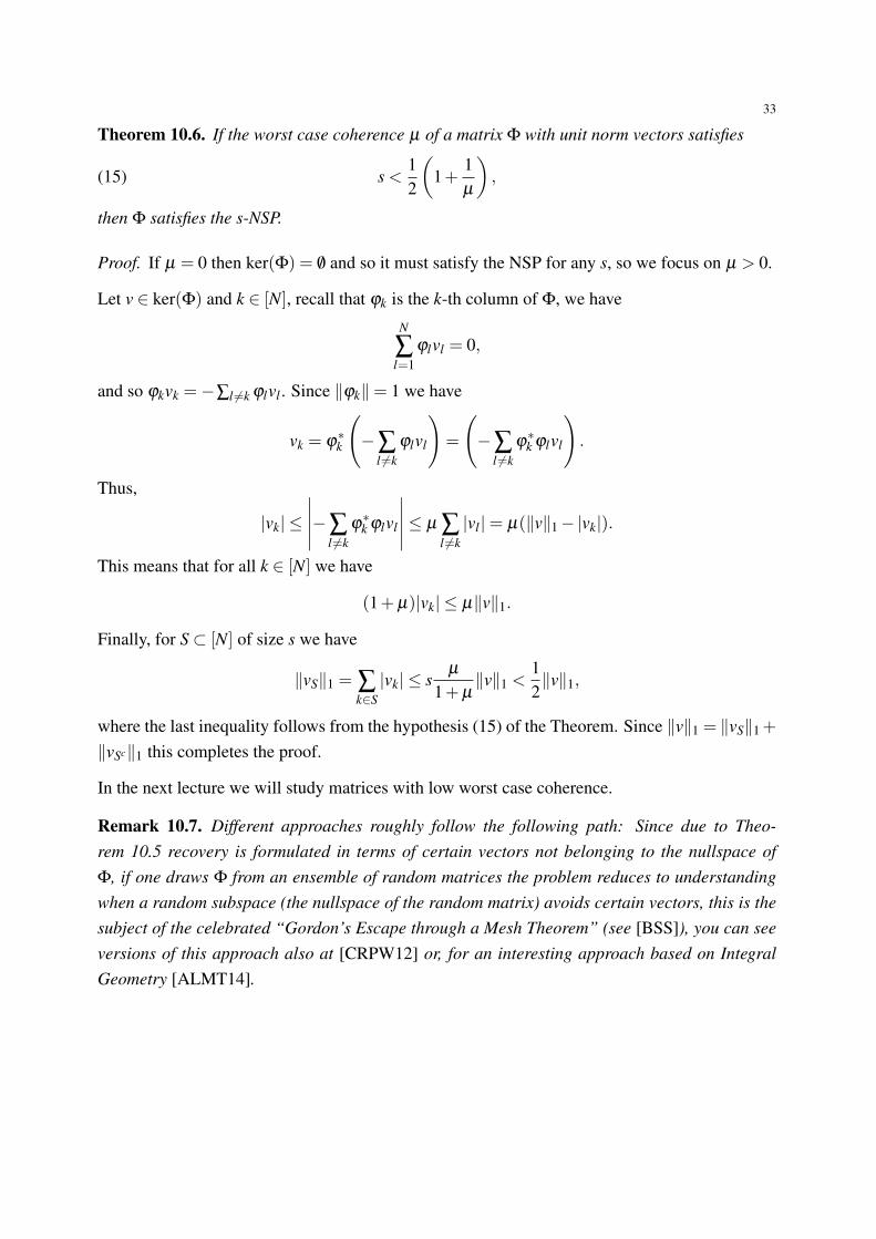
Theorem 10.6. If the worst case coherence µ of a matrix Φ with unit norm vectors satisfies
(15) s <12
(1+
1µ
),
then Φ satisfies the s-NSP.
Proof. If µ = 0 then ker(Φ) = /0 and so it must satisfy the NSP for any s, so we focus on µ > 0.
Let v ∈ ker(Φ) and k ∈ [N], recall that ϕk is the k-th column of Φ, we have
N
∑l=1
ϕlvl = 0,
and so ϕkvk =−∑l 6=k ϕlvl . Since ‖ϕk‖= 1 we have
vk = ϕ∗k
(−∑
l 6=kϕlvl
)=
(−∑
l 6=kϕ∗k ϕlvl
).
Thus,
|vk| ≤
∣∣∣∣∣−∑l 6=k
ϕ∗k ϕlvl
∣∣∣∣∣≤ µ ∑l 6=k|vl|= µ(‖v‖1−|vk|).
This means that for all k ∈ [N] we have
(1+µ)|vk| ≤ µ‖v‖1.
Finally, for S⊂ [N] of size s we have
‖vS‖1 = ∑k∈S|vk| ≤ s
µ
1+µ‖v‖1 <
12‖v‖1,
where the last inequality follows from the hypothesis (15) of the Theorem. Since ‖v‖1 = ‖vS‖1+
‖vSc‖1 this completes the proof.
In the next lecture we will study matrices with low worst case coherence.
Remark 10.7. Different approaches roughly follow the following path: Since due to Theo-rem 10.5 recovery is formulated in terms of certain vectors not belonging to the nullspace ofΦ, if one draws Φ from an ensemble of random matrices the problem reduces to understandingwhen a random subspace (the nullspace of the random matrix) avoids certain vectors, this is thesubject of the celebrated “Gordon’s Escape through a Mesh Theorem” (see [BSS]), you can seeversions of this approach also at [CRPW12] or, for an interesting approach based on IntegralGeometry [ALMT14].

34
11. LOW COHERENCE FRAMES (01.04.2021)
Motivated by Theorem 10.6 in this section we study the worst-case coherence of frames with thegoal of understanding how much savings (in measurements) one can achieve with the techniquedescribed last section. We start with a lower bound.
Theorem 11.1 (Welch Bound). Let ϕ1, . . . ,ϕN ∈ Cd be N unit norm vectors (‖ϕk‖ = 1). Let µ
be their worst case coherenceµ = max
i 6= j
∣∣〈ϕi,ϕ j〉∣∣ .
Then
µ ≥
√N−d
d(N−1)
Proof. Let G be the Gram matrix of the vectors, Gi j = 〈ϕi,ϕ j〉=ϕ∗i ϕ j. In other words, G=Φ∗Φ.It is positive semi-definite and its rank is at most d. Let λ1, . . . ,λd denote the largest eigenvaluesof G, in particular this includes all non-zero ones. We have
(TrG)2 =
(d
∑k=1
λk
)2
≤ dd
∑k=1
λ2k = d
N
∑k=1
λ2k = d‖G‖2
F ,
where the inequality follows from Cauchy-Schwarz between the vectors with the λk’s and theall-ones vector.
Note that since the vectors are unit normed, Tr(G) = N, thus
N
∑i, j=1|〈ϕi,ϕ j〉|2 = ‖G‖2
F ≥1d(TrG)2 =
N2
d.
Also,N
∑i, j=1|〈ϕi,ϕ j〉|2 =
N
∑i=1|〈ϕi,ϕi〉|2 +
N
∑i6= j|〈ϕi,ϕ j〉|2 = N +
N
∑i 6= j|〈ϕi,ϕ j〉|2 ≤ N +(N2−N)µ2.
Putting everything together gives:
µ ≥
√N2
d −N(N2−N)
=
√N−d
d(N−1).
2
Remark 11.2. We used C for the Theorem above since it also follows for a frame in Rd by simplyviewing its vectors as elements of Cd .

35
Remark 11.3. Notice that in the proof above there were two inequalities used, if we track thecases when they are “equality” we can see for which frames the Welch bound is tight. TheCauchy-Scwartz inequality is tight when the vector consisting in the first d eigenvalues of Gis a multiple of the all-ones vector, which is the case exactly when Φ is a Tight Frame (recallDefinition 8.3). The second inequality is tight when all the terms in the sum ∑
Ni6= j |〈ϕi,ϕ j〉|2 are
equal. The frames that satisfy these properties are called ETFs – Equiangular Tight Frames.
Definition 11.4 (Equiangular Tight Frame). A unit-normed Tight frame is called an EquiangularTight Frame if there exists µ such that, for all i 6= j,
|〈ϕi,ϕ j〉|= µ.
Proposition 11.5. Let ϕ1, . . . ,ϕN by an equiangular tight frame in Kd then
• If K= C then N ≤ d2
• If K= R then N ≤ d(d+1)2 .
Proof. Let ψi = vec(ϕiϕ∗i ), these vectors8 are unit norm and their inner products are
ψ∗i ψ j = 〈vec(ϕiϕ
∗i ) ,vec
(ϕ jϕ
∗j)〉= Tr
((ϕiϕ
∗i )∗ (
ϕ jϕ∗j))
= |〈ϕi,ϕ j〉|2 = µ2.
This means that their Gram matrix H is given by
H =(1−µ
2) I +µ211T .
Since µ 6= 1 we have rank(H) = N. But the rank needs to be smaller or equal than the dimensionof the ϕi’s which
• For Cd is at most d2,• For Rd , due to symmetry it is at most 1
2d(d +1).
Thus N ≤ d2 for K= C, and N ≤ d(d+1)2 for K= R. 2
Further Reading 11.1. Equiangular Tight Frames in Cd with N = d2 are important objects isQuantum Mechanics, where they are called SIC-POVM: Symmetric, Informationally Complete,Positive Operator-Valued Measure. It is a central open problem to prove that they exist in alldimensions d, see Open Problem 6.3. in [Ban16] (the conjecture that they do exist is known asZauner’s Conjecture).
8vec(M) for a matrix M corresponds to the vectors formed by the entries of M; in this case it is not importanthow the indexing is done as long as consistent throughout.

36
While constructions of Equiangular Tight Frames are outside the scope of this course,9 there aresimple families of vectors with worst case coherence µ ∼ 1√
d: Let F ∈ Cd×d denote the Discrete
Fourier Transform matrix
Fjk =1√d
exp [−2πi( j−1)(k−1)/d] .
F is an orthonormal basis for Cd . Notably any column of F has an inner product of 1√d
with thecanonical basis, this means that the d×2d matrix
(16) Φ = [I F ]
has worst case coherence 1√d
.
Theorem 10.6 guarantees that, for Φ given by (16), `1 achieves exact recovery for sparsity levels
s <12
(1+√
d).
Remark 11.6. There are many constructions of unit norm frames with low coherence, with re-dundancy quotients (N/d) much larger than 2. There is a all field of research involving theseconstructions, there is a “living” article keeping track of constructions [FM]. You can also takea look at the PhD thesis of Dustin Mixon [Mix12] which describes part of this field, and discussesconnections to Compressed Sensing; Dustin Mixon also has a blog in part devoted to these ques-tions [Mix]). We will not discuss these constructions here, but Exploratory Challenge 11.4 willshow that even randomly picked vectors do quite well (we will do this at the end of the course, aswe need some of the probability tools introduced later on).
Definition 11.7. Construction (16) suggest the notion of Mutually Unbiased Bases: Two or-thonormal bases v1, . . . ,vd and u1, . . . ,ud of Cd are called Mutually Unbiased if for all i, j wehave |v∗i u j|= 1√
d. A set of k bases are called Mutually Unbiased if every pair is Mutually Unbi-
ased.
Challenge 11.2. Show that a matrix formed with two orthonormal bases such as (16) cannothave worst case coherence smaller than 1√
d.
Further Reading 11.3. Mutually Unbiased basis are an important object in quantum mechan-ics, communication, and signal processing, however there is still that is not understood aboutthem. My favourite question about them is: “How many mutually unbiased basis exist in 6 di-mensions”? The best known upper bound is 7 (d +1 is always an upper bound, and is known tobe tight for prime powers but not in general), the best known lower bound for 6 dimensions is 3.See Open Problem 6.2. in [Ban16].
9I should point out though that there are fascinating connections with Number Theory, Graph Theory, and otherareas.

37
Exploratory Challenge 11.4. This Challenge is special, it is meant to be solved later in thecourse (we will likely put it in the homework). Towards the end of the course, equiped with a fewmore tools of Probability, you’ll be able to show that by simply taking a frame made up of random(independent) vectors in the unit norm sphere, the coherence is comparable to the Welch bound,in particular you will show that N such vectors in d dimensions will have worst case coherencepolylog(N)√
d, where polylog(N) means a polynomial of the logarithm of N (you will also work out
the actual dependency).
Further Reading 11.5. Turns out that with matrices consisting of random (independent) columns,one can perform sparse recovery with `1 minimization for much larger levels of sparsity (s. d
log(n)
rather than s.√
d). Proving this however is outside the scope of this course, as it requires heav-ier Probability Theory machinery. Interestingly, matching this performance with deterministicconstructions seems notoriously difficult, in fact there is only one known construction “breakingthe square-root bottleneck”. You can read more about this in Open Problem 5.1. in [Ban16] (andreferences therein).

38
12. MATRIX COMPLETION & RECOMMENDATION SYSTEMS (01.04.2021)
Recommendation Systems is a central application in Machine Learning. In this Section we willfocus on the problem of Matrix Completion and will use the Mathematics we developed in thelast few sections to motivate algorithms for this problem; while an analysis of these algorithms isoutside the scope of this course, they are essentially analogues of the ones developed for sparserecovery. This section, which concludes the first half of the course, is less technical than the previ-ous noes, and more devoted to describing algorithms and applications (and some “story-telling”).Nonetheless we will include a guarantee for matrix completion as a “delayed” homework, as itwill be doable with techniques available at the end of the course.
12.1. Netflix Prize. The problem of matrix completion is often referred to as the Netflix prob-lem. This is because a bit over a decade ago Netflix launched a contest to improve their rec-ommendation algorithm; teams could have access to a training data set and propose algorithms,the winning team (based on performance on an unseen test data set) received 1 Million dollars.This lasted a few years and it is quite an incredible story. I couldn’t possibly describe it herebetter than the professional press outlets, so I recommended taking a look at the context website:https://netflixprize.com/index.html
You can also access the data here:
https://www.kaggle.com/netflix-inc/netflix-prize-data
Exploratory Challenge 12.1. I recommend, if you find the time, to try simple algorithms on thisdataset!
Here are a few articles with more information, it is quite the story!
https://www.thrillist.com/entertainment/nation/the-netflix-prize
https://www.wired.com/2009/09/how-the-netflix-prize-was-won/
https://en.wikipedia.org/wiki/Netflix_Prize
12.2. The Problem. Let’s use the Netflix problem as the driving example. Let M ∈Rn×m denotethe matrix of user/movie ratings (say in either±1 or 1−−5 ratings), the goal is to estimate unseenentries of M from a few observed entries. Much like the sparse recovery problem above, this isimpossible without (parsimony) assumptions on M. A classically used assumption is that M islow rank (movies and users can be well described as linear combinations of a few “factors”). TheMathematical probelm then becomes:

39
Problem 12.1 (Low Rank Matrix Completion). Recover M ∈ Rn×m a low rank matrix (meaningrank(M)≤ r for r n,m) from observations Ω⊂ [n]× [m]:
Mi j = yi j, for (i, j) ∈Ω
Central questions include
• How large does Ω need to be?• What are efficient algorithms?
We will discuss the second question first, you can see [H+15] for a nice discussion relating thetwo algorithms we discuss here. A particularly simple algorithm is motivated by the first part ofthe course, where we discussed truncated SVD. The idea is to start by setting all non-observedentries to 0, and then update the estimator M by repeatedly alternative through the following twoiterations
(1) Perform truncated SVD on M(2) “Correct” the observed Ω entries of M to coincide with the observations.
Both iteration (1) will in general change the entries in Ω and iteration (2) will in general increasethe rank of M, so they need to be performed until convergence (or a stopping criteria is satisfied).
12.3. Nuclear Norm Minimization. Another algorithm appears as a natural generalization of`1 minimization for sparse recovery. Since M is low rank, the vectors of singular values of M,σ(M) is sparse. The tools developed in the sections above suggest minimizing the `1 norm ofσ(M), which we have seen is the Schatten-1 norm of M (recall Definition 4.3). This suggests thefollowing optimization problem
(17)min ‖M‖(S,1)s.t. Mi j = yi j for all (i, j) ∈Ω
This is known in the literature as Nuclear Norm miminization and is known to recover a low rankmatrix M, under certain incoherence assumptions, from only r(m+ n)polylog(n+m) observa-tions (note that if r is small this is significantly smaller than n×m). While guarantees for thisalgorithm are outside the scope of this course, as they require tools from random matrix theory,we point out that the key reasons for the success of the algorithm are analogous to the ones for `1
minimization in sparse recovery. There is a fascinating line of work establishing guarantees forthis algorithm [CT10, CR09, Rec11, Gro11]. We point out that solving (17) is indeed efficient, itis a so called Semidefinite Program [VB04].
40
12.4. Guarantees. Here we discuss a guarantee for a particularly simple, but already mathemat-ically rich, example. Let us consider the case of r = 1, thus M = uvT for some unknown vectors uand v. Let us assume further that u and v have only non-zero entries (this is a particularly strongversion of the “incoherence assumptions” mentioned above). We are interested in understandingwhen is it that M is uniquely determined by the set of observations Ω⊂ [n]× [m], we will relateit with the connectivity of a a certain graph.
Recall that a bipartite graph is a graph with two sets of nodes such that all edges have an endpointin each of the sets. Given the set Ω consider the graph GΩ to be the bipartite graph on n+mnodes (corresponding to rows and columns of M) where node i ∈ [n] and j ∈ [m] are connected ifand only if i, j ∈Ω.
Theorem 12.2. A matrix M = uvT , with u and v both vectors in no zero entry, is uniquely deter-mined by the entry values in Ω⊂ [n]× [m] if and only if GΩ is connected.
Challenge 12.2. Prove this Theorem.
As a homework problem layer in the course, you will show that roughly (m+n) log(m+n) entriesindependently picked at random are enough to uniquely determine M.
Exploratory Challenge 12.3. A bipartite Erdos-Renyi random graph G(n,m, p) is a bipartitegraph on n+m nodes where every possible edge between the first n nodes and the last m nodesappears, independently, with probability p. For which values of p is the graph connected withhigh probability? (Similarly to Exploratory Challenge 11.4, this is meant to be solved later in thecourse, when posted as homework it will contain more information and “stepping stones”).
Exploratory Challenge 12.4. This result for random graph is more classical on not necessarilybipartite graphs (which would correspond to a symmetric version of the matrix completion prob-lem). An Erdos-Renyi random graph G(n, p) is a graph on n nodes where every possible edgeappears, independently, with probability p. For which values of p is the graph connected withhigh probability? (Similarly to Exploratory Challenge 11.4, this is meant to be solved later in thecourse, when posted as homework it will contain more information and “stepping stones”).
Remark 12.3. Although the connection with random matrix theory won’t be discussed here, itlikely will not be a complete surprise at this point, given that connectivity of a graph is related toproperties of the corresponding adjacency matrix. In the rank 1 case, there is no need for randommatrix theory and considerably simpler tools from probability theory will suffice.

41
13. CLASSIFICATION THEORY: FINITE CLASSES (15.04.2021)
Theory of Classification is a foundational topic in Statistical Machine Learning. The directionwe are discussing in this part of the course was initiated by Vladimir Vapnik and Alexey Chervo-nenkis in the mid-60s and independently by Leslie Valiant in the mid-80s. The results of Vapnikand Chervonenkis lead to what we now call Vapnik–Chervonenkis Theory. From the early 70sto the present day, their work has an ongoing impact on Machine Learning, Statistics, EmpiricalProcess Theory, Computational Geometry and Combinatorics. In parallel, the work of Valiantlooked at a similar problem from a more computational perspective. In particular, Valiant de-veloped the theory of Probably Approximately Correct (PAC) Learning that lead, among othercontributions, to his 2010 Turing Award.
In this part of the course, we study the following simple model. We are given a sequence ofindependent identically distributed observations
X1, . . . ,Xn
taking their values in X ⊆ Rp such that each Xi is distributed according to some unknown dis-tribution P 10. In our case each Xi might be seen as an image or a feature vector. For example,consider the problem of health diagnostics. In this case these vectors can describe some medicalinformation such as age, weight, blood pressure and so on. An important part of our analysisis that the dimension of the space will not play any role, and classification is possible even inabstract measurable spaces.
In contrast to clustering problems discussed earlier, we also observe labels
f ∗(X1), . . . , f ∗(Xn),
where f ∗ is an (unknown to us) target classifier mapping Rp→ 0,1. Depending on a partic-ular problem, these labels can represent spam/not spam when classifying the emails, disease/nodisease when diagnosing the patient and so on. Of course, we put a standard measurability as-sumption on f ∗ so that e.g., f ∗(x) = 1 is measurable. Using the labeled sample
(18) Sn = ((X1, f ∗(X1)), . . . ,(Xn, f ∗(Xn)))
our aim is to construct a measurable classifier f : X → 0,1 that can be used to classify anyfurther element x ∈ X . The risk or the error of a (measurable) classifier f : X → 0,1 isdefined by
R( f ) = Pr( f (X) 6= f ∗(X)).
10We assume that there is a probability space (X ,F,P), where F is a Borel σ -algebra.

42
With this definition in mind, we want to consider classification rules that have their risk as smallas possible. Our second assumption is that f ∗ belongs to some known class F of (measurable)classifiers mapping X to 0,1. We remark that in the Computer Science literature these classi-fiers are usually called concepts.
Definition 13.1. We say that a classifier f is consistent with the sample Sn if for all i = 1, . . . ,n,
f (Xi) = f ∗(Xi).
Observe that to find a consistent classifier one should observe the labeled sample Sn, but no otherknowledge (except the fact that f ∗ ∈F ) on f ∗ is required.
Before presenting our next result, let us give its informal description. Given the sample Sn, themost natural way is to choose any f ∈F consistent with it. Our hope is that this classifier willlikely be close to the true classifier f ∗. Since the sample Sn is random, we cannot guaranteethis definitely. Instead, we may only say that f is close to f ∗ with high probability: this wouldmean intuitively that for a large fraction of all random realizations of the sample Sn, any classifierconsistent with a particular realization of the sample has a small risk. There is an alternative andequivalent way of looking at this. Instead of saying that with high probability any classifier thatis consistent with the sample has a small risk, one may argue that any classifier that has a largerisk cannot be consistent with the sample Sn. The latter idea will be central in our proofs.
Theorem 13.2. Assume that f ∗ ∈F , and F is finite. For the confidence parameter δ ∈ (0,1)and the precision parameter ε ∈ (0,1) fix the sample size
n≥⌈
log |F |ε
+1ε
log1δ
⌉.
Let f be any classifier in F consistent with the sample Sn. Then,
(19) Pr(X1,...,Xn)
(R( f )< ε
)≥ 1−δ .
Equivalently, with probability at least 1− δ , any classifier f such that its risk is larger than ε
(that is, R( f )> ε) cannot be consistent with the sample Sn.
Although our proofs are usually based on the second principle, we present our result in the shortform (19).

43
Proof. We follow the strategy discussed above. Fix any f ∈ F such that R( f ) = Pr( f (X) 6=f ∗(X))≥ ε . We have,
Pr(X1,...,Xn)
( f (Xi) = f ∗(Xi) for i = 1, . . . ,n)
=n
∏i=1
PrXi( f (Xi) = f ∗(Xi))
=n
∏i=1
(1−PrXi( f (Xi) 6= f ∗(Xi)))
≤ (1− ε)n
≤ exp(−nε),
where in the last line we used 1− x ≤ exp(−x). Recall the union bound: for a set of eventsA1, . . . ,Ak we have Pr(A1∪ . . .∪Ak)≤ ∑
ki=1 Pr(Ai). Now, using the union bound we have
Pr(X1,...,Xn)
(there is f ∈F , R( f )≥ ε such that f (Xi) = f ∗(Xi) for i = 1, . . . ,n)
≤ ∑f∈F
Pr(X1,...,Xn)
(R( f )≥ ε and f (Xi) = f ∗(Xi) for i = 1, . . . ,n)
≤ |F |exp(−nε),
where the last line follows from our bound for a single fixed classifier. We want this probabilityto be small. We set |F |exp(−nε) = δ . Therefore, it is sufficient to take the sample size
n =
⌈log |F |
ε+
1ε
log1δ
⌉to guarantee that, with probability at least 1−δ , any classifier f ∈F consistent with the samplehas its risk smaller than ε . Indeed, if n is chosen this way, we have
Pr(X1,...,Xn)
(there is f ∈F , R( f )≥ ε such that f (Xi) = f ∗(Xi) for i = 1, . . . ,n)≤ δ .
Taking the complementary event proves the claim.
One may rewrite the result of Theorem 13.2 as a risk bound. That is, we first fix the sample size nand want to estimate the precision ε of our classifier. Repeating the lines of the proof of Theorem13.2, we have for any f consistent with Sn,
Pr(X1,...,Xn)
(R( f )≤ log |F |
n+
1n
log1δ
)≥ 1−δ .
The result of Theorem 13.2 inspires the following definition. In what follows, PAC stands forProbably Approximately Correct. Indeed, we showed that for any finite class F any sampleconsistent classifier is approximately correct (risk ≤ ε) with high probability.

44
Definition 13.3. A (possibly infinite) class F of classifiers is PAC-learnable with the samplecomplexity n(δ ,ε) if there is a mapping A : ∪∞
m=0(X ×0,1)m→0,1X (called the learningalgorithm; given a sample S of any size it outputs a classifier A(S)) that satisfies the followingproperty: for every distribution P on X , every δ ,ε ∈ (0,1) and every target classifier f ∗ ∈F ,if the sample size n is greater or equal than n(δ ,ε), then
Pr(X1,...,Xn)
(R(A(Sn))≤ ε)≥ 1−δ .
Remark 13.4. When considering finite classes we have little problems with measurability andwe may only request that for all f ∈F the set f (x) = 1 is measurable. The notion of PAC-learnability allows infinite classes. In this case the question of measurability is more subtle.However, as a rule of thumb, one may argue that measurability issues will almost never appearin the analysis of real-life algorithms. In particular, starting from late-80s there is a usefuland formal notion of well-behaved classes: these are essentially the classes for which thesemeasurability issues do not appear. We add some clarifying references thought the text.
An immediate outcome of Theorem 13.2 is the following result.
Corollary 13.5. Any finite class F is PAC learnable with the sample complexity
n =
⌈log |F |
ε+
1ε
log1δ
⌉.
Moreover, to learn this class, we simply need to output any consistent classifier f .
14. PAC-LEARNING FOR INFINITE CLASSES: STABILITY AND SAMPLE COMPRESSION
(15.04.2021)
An important limitation of Theorem 13.2 is that it only deals with finite classes. Working onlywith discrete spaces of solutions is also somewhat impractical: many modern machine learningtechniques are based on the gradient descent methods that require that the class F is parametrizedin a relatively smooth way by Rp. In order to analyze infinite sets F , we can use the followingsimple argument that can be again attributed to Vapnik and Chervonenkis. Given f ∗ ∈F , con-sider a non-random labeled sample of size n+1:
sn+1 = (x1, f ∗(x1)), . . . ,(xn+1, f ∗(xn+1)).
We use lowercase s to emphasize that this sample is non-random. For i = 1, . . . ,n+1, let
sin+1 = S\(xi, f ∗(xi)).
45
That is, we removed the i-th observation from the sample S. Let A be any learning algorithm, anddenote f i = A(si
n+1). The Leave-One-Out error (LOO) is defined by
LOOA = LOOA(sn+1) =1
n+1
n+1
∑i=1
1 f i(xi)6= f ∗(xi),
where as before 1E is an indicator of E. It is easy to see how LOO works: one by one we removethis instances from the sample, construct a new classifier and test its performance on the removedpoint. Even though the Leave-One-Out error is deterministic, we may also look at it as a randomvariable by replacing all xi by corresponding independent identically distributed Xi-s.
Theorem 14.1. For any learning algorithm A,
EX1,...,XnR(A(Sn)) = EX1,...,Xn+1 LOOA(Sn+1).
Proof. Since the random variables X1, . . . ,Xn+1 are independent and identically distributed, theterms in the sum
LOOA(Sn+1) =1
n+1
n+1
∑i=1
1 f i(Xi)6= f ∗(Xi)
have the same distribution. Therefore, the expected values of each summand are the same. Bythe linearity of expectation, we have
1n+1
EX1,...,Xn+1
n+1
∑i=1
1 f i(Xi)6= f ∗(Xi)= EX1,...,Xn+11 f n+1(Xn+1)6= f ∗(Xn+1)
.
Using the independence of X1, . . . ,Xn+1, we first take the expectation only with respect to Xn+1
(one may formally use either the conditional expectation argument or the Fubini theorem). Thisimplies
EX1,...,Xn+11 f n+1(Xn+1)6= f ∗(Xn+1)= EX1,...,XnR( f n+1) = EX1,...,XnR(A(Sn)).
The claim follows.
Example 14.2. Learning axis-aligned rectangles. The following simple example can be describedin words. Consider the class of classifiers F induced by axis-aligned rectangles in R2: that is,for each axis-aligned rectangle we build a classifier that labels its interior and border by 1 and itsexterior by 0. Assume that some unknown target rectangle f ∗ ∈F is chosen. We need to describeour learning algorithm. Let the classifier f correspond to the smallest axis-aligned rectangle thatcontains all instances labeled by 1. It is easy to check that for any deterministic sample of size n:
LOOA(sn+1)≤4
n+1.

46
Indeed, f i can be wrong only when removing an instance with the label 1 on the border of thedescribed classifier trained on sn+1. Thus, by Theorem 14.1 we have
EX1,...,XnR( f )≤ 4n+1
.
Challenge 14.1. Using Example 14.2, prove directly that the class of axis-aligned rectangles isPAC-learnable.
One of the drawbacks of Theorem 14.1 is that it only controls the expected risk. We show thatthe ideas used in Example 14.2 can be used in full generality in order to provide high probabilitysample complexity bounds. Observe that the rectangle f in Example 14.2 is defined by the fourinstances that belong to its border. In particular, if we remove all instances in the sample exceptthese four, then the same classifier f is constructed. Moreover, this classifier will correctly labelthe original learning sample. In some sense, we compress the information stored in the sampleinto a small subsample. This motivates the following definition.
Definition 14.3. Consider a pair of functions: a compression function
κ : ∪∞m=0(X ×0,1)m→∪∞
m=0(X ×0,1)m
(it is a function mapping a sample to a subsample of size `) and a reconstruction function
ρ : ∪∞m=0(X ×0,1)m→0,1X

47
(it maps labeled samples to classifiers). The pair (ρ,κ) defines the sample compression schemeof size ` for F if the following holds for any f ∗ ∈ F , any integer n and any sample sn =
((x1, f ∗(x1), . . . ,(xn, f ∗(xn))):
• it holds that κ(sn) ⊆ sn. That is, compression functions always map to a subset of theoriginal sample;• the size of a compression set satisfies |κ(sn)| ≤ `;• the classifier f = ρ(κ(sn)) satisfies for all i = 1, . . . ,n, f (xi) = f ∗(xi). That is, the re-
construction function applied to the compression set recovers the labels of sn. In otherwords, f is consistent with the sample sn.
Example 14.4. Check that Example 14.2 defines a sample compression scheme of size `= 4.
Of course, when considering statistical guarantees we always assume that ρ outputs a measurableclassifier.
Theorem 14.5. Assume that F admits a sample compression scheme (ρ,κ) of size ` and that ρ
is permutation invariant (does not depend on the order of input instances). For the confidenceparameter δ ∈ (0,1) and the precision parameter ε ∈ (0,1), fix the sample size
n≥ `+
⌈`
εlog
en`+
1ε
log1δ
⌉.
Then, for the classifier f = ρ(κ(Sn)), it holds that
Pr(X1,...,Xn)
(R( f )≤ ε)≥ 1−δ .
Proof. The proof is similar to the proof of Theorem 13.2. Consider without loss of generalitythe first ` elements of Sn. This set is denoted by S`. This corresponds to the naive compressionfunction κ that always maps to the first ` instances of Sn. Using the same arguments as in Theorem13.2 we have (conditioned on X1, . . . ,X`)
PrX`+1,...,Xn
(R(ρ(S`))≥ ε and ρ(S`)(Xi) = f ∗(Xi) for i = `+1, . . . ,n)≤ exp(−ε(n− `)).
Observe that this probability will only decrease if S` is replaced by Sk,k < `. Our idea is to provethe statement no matter which subset is selected by κ . Indeed, by our assumption κ always mapsto one of at most (provided that n≥ `)
`
∑j=0
(nj
)≤(en`
)`
48
subsets and since ρ is permutation invariant, we ignore the order of the elements in the corre-sponding set. To verify the last inequality we use
d
∑j=0
(nj
)≤
d
∑j=0
(ni
)(nd
)d− j≤
n
∑j=0
(ni
)(nd
)d−i=(n
d
)d(
1+dn
)n
≤(en
d
)d,
where we used the binomial theorem. Therefore, by the union bound, no matter which subset isselected by the compression function κ , we have
PrX`+1,...,Xn
(R(ρ(κ(Sn)))≥ ε)
≤(en`
)`EX1,...,X`
PrX`+1,...,Xn
(R(ρ(S`))≥ ε and ρ(S`)(Xi) = f ∗(Xi) for i = `+1, . . . ,n)
≤(en`
)`exp(−ε(n− `)).
The sample complexity bound follows by a simple computation.
Challenge 14.2. Prove an analog of Theorem 14.5 in the case where ρ is not permutation invari-ant.
Observe that the existence of a sample compression scheme of finite size implies PAC-learnability.Sample compression is a source of several major open problem in Learning Theory. We discusssome of them later.
Remark 14.6. One may prove the following identity: for α,β ,γ > 0,n≥ 1 if αβeγ/α > 2, then
n > 2γ +2α ln(αβ ) implies n > γ +α log(βn).
See Corollary 4.1 in [Vid13]. Therefore, it is easy to verify that our requirement n> `+ `ε
log en` +
1ε
log 1δ
can be replaced by
(20) n > 2`+2`ε
logeε+
2ε
log1δ,
The last condition does not contain n in the right-hand side.
Further Reading 14.3. Theorem 13.2 and the model we are studying appears in the work ofVapnik and Chervonenkis [VC64a]. This work also provides a matching lower bound. See also[Cov65b]. The work of Valiant [Val84] introduces the formal notion of PAC-learnability. Theo-rem 14.1 appears explicitly in the first textbook of Vapnik and Chervonenkis [VC74], though theargument was known in the mid-60s. See additional historical remarks on this result in [VPG15,Chapter I]. Theorem 14.5 is essentially due to Littlestone and Warmuth [LW86]. Another recom-mended reference with many related discussions is [HR21].

49
15. PERCEPTRON (22.04.2021)
In this lecture, we analyze the Perceptron algorithm. This algorithm was invented in the late-50sby Frank Rosenblatt. Even though it is one of the first learning algorithms, Perceptron has closerelations to multiple foundational methods and principles such as stochastic gradient descentand sample compression schemes. Later in our course, we also make a connection with onlinelearning. Moreover, Perceptron is a building block of artificial neural networks.
For notational convenience, we work with the labels −1,1 instead of 0,1 when consideringthe Perceptron algorithm.
Definition 15.1. We say that a set of labeled vectors W ⊂Rp×1,−1 is linearly separable witha margin γ if there is a vector v ∈Rp such that for any (x,y) ∈W, where x ∈Rp and y ∈ 1,−1,it holds that
y〈v,x〉‖v‖
≥ γ.
The intuition behind the margin is as follows. From linear algebra we know that the distancefrom x to the separating hyperplane induced by v is equal to
|〈v,x〉|‖v‖
.
The margin assumption means that each (x,y) lives in a half-space corresponding to its label yand the distance from x to the separating hyperplane is at least γ . In fact, for any vector w ∈ Rp
there is a natural way to define a classifier: we consider the mapping x 7→ sign(〈w,x〉). That is,the vector w induces a half-space and is orthogonal to the separating hyperplane. In particular, wmisclassifies x ∈ Rp whenever
y〈w,x〉 ≤ 0.
Remark 15.2. For the sake of simplicity, in this lecture we focus on homogenous half-spaces.That is, we assume that the separating hyperplane passes through the origin.
Our first aim will be the following: given a linearly separable sample of labeled vectors sn =
(x1,y1), . . . ,(xn,yn), find a vector w that certifies this linear separability. The following algo-rithm is aiming to do so.
Perceptron Algorithm.
• Input: sn = (x1,y1), . . . ,(xn,yn).• Set w1 = 0.• For i = 1, . . . ,n do

50
(1) If yi〈wi,xi〉 ≤ 0(2) wi+1 = wi + yixi,(3) Else(4) wi+1 = wi,
• Return: wn+1.
The simplest interpretation of this algorithm is as follows. Whenever wi misclassifies xi, weupdate it by using the rule wi+1 = wi + yixi. This implies, in particular, that
yi〈wi+1,xi〉= yi〈wi,xi〉+ y2i ‖xi‖2 = yi〈wi,xi〉+‖xi‖2.
The additional positive term ‖xi‖2 implies that wi+1 is less likely to misclassify xi. The next resultis the basic error bounds for the Perceptron algorithm.
Theorem 15.3. Assume that we are given a finite set of labeled vectors sn = (x1,y1), . . . ,(xn,yn)in Rp that is linearly separable with a margin γ . Let max
i=1,...,n‖xi‖ ≤ r, for some r > 0. The number
of updates (misclassifications) made by the Perceptron algorithm when processing sn is boundedby r2/γ2. This values does not depend on n.
Proof. Let J ⊆ 1, . . . ,n denote the set of indexes where the Perceptron algorithm updates theweight vector. By y〈v,x〉
‖v‖ ≥ γ and the linearity of the inner product, we have
|J|γ ≤∑i∈J
yi〈v,xi〉‖v‖
.
By the Cauchy-Schwarz inequality and the definition of the update rule we obtain
∑i∈J
yi〈xi,v〉‖v‖
≤
∥∥∥∥∥∑i∈Jyixi
∥∥∥∥∥=∥∥∥∥∥∑i∈J
(wi+1−wi)
∥∥∥∥∥= ‖wmax(J)+1‖,
where in the last line equality we used telescopic sums (with w1 = 0). Further, using telescopicsums again, we have
‖wmax(J)+1‖=√
∑i∈J
(‖wi+1‖2−‖wi‖2)
=√
∑i∈J
(‖wi + yixi‖2−‖wi‖2)
≤√
∑i∈J
(2yi〈wi,xi〉+‖xi‖2) (since yi〈wi,xi〉 ≤ 0)
≤√
∑i∈J‖xi‖2 ≤
√|J|r2.

51
Therefore, we have
|J|γ ≤√|J|r2 =⇒ |J| ≤ r2/γ
2.
The claim follows.
Observe that we only restrict the norms of the vectors that correspond to the instances misclassi-fied by the Perceptron algorithm. These instances are usually called the support vectors. We areready to show that these support vectors define a sample compression scheme.
Proposition 15.4. Consider the case of linearly separable data with a margin γ and such that thenorms of the vectors are restricted to the ball of radius r. Then, the Perceptron algorithm definesa sample compression scheme of size `≤ r2/γ2.
Proof. The exposition of the proof is again simplified if we present it informally. We first needto order the vectors in Rp. For any x,y ∈ Rp we write x ≺ y if x j < y j, where j ∈ 1, . . . , pis the first index where x j 6= y j. Given a learning sample sn, we always first sort the instancesin ascending order according to ≺. Consider running the Perceptron algorithm through sn andcycling through this ordered set repeatedly until it makes a full pass through it without makingany mistakes. This procedure will surely terminate since the sample sn is finite, and by Theorem15.3, we only make a finite number of mistakes on a sample of arbitrary length.
Let s∗n⊆ sn denote the set of mistakes of the Perceptron algorithm executed as above. By Theorem15.3 we have |s∗n| ≤ r2/γ2. Therefore, the Perceptron algorithm defines a compression function ofsize `≤ r2/γ2. This function maps sn to s∗n. We only need to construct a reconstruction function.Fix any x ∈Rp that does not have a labeled copy in s∗n. We put the unlabeled x among s∗n and sortthem according ≺. We run the Perceptron algorithm on the ordered set s∗n ∪x until the labelof x is determined. That is, the label of x is sign(〈x,w〉), where w is the current vector when x isprocessed. For any x that has a copy in s∗n we return its correct label. Indeed, in this case the labelof x is stored in s∗n. This defines (point-wise) the reconstruction function. By our construction forany x ∈ sn its label will be correctly classified by this reconstruction function. Thus, we defineda sample compression scheme of size `≤ r2/γ2.
Challenge 15.1. Make this proof formal.
Challenge 15.2. Prove that alternatively one may use the following reconstruction function: runthe Perceptron algorithm through s∗n and cycling through this ordered set repeatedly until it makesa full pass through it without making any mistakes. Any new point x is now classified by the finaloutput vector w. Argue that in this case ρ(κ(Sn)) matches the output of the Perceptron algorithmtrained until it passes through Sn without making any mistakes.
Remark 15.5. For the reconstruction function of Proposition 15.4 one may use a compressionfunction making only a single pass through the sample.

52
Thus, in our setup the sample complexity bound (20) implies that if the sample size
n >2r2
γ2 +2r2
γ2εlog
eε+
2ε
log1δ,
then the output classifier w of the Perceptron-based sample compression scheme of Proposition15.4 satisfies
Pr(X1,...,Xn)
(R(w)≤ ε)≥ 1−δ .
Challenge 15.3. Verify that the Leave-One-Out argument (Theorem 14.1) can also be used toprovide an in-expectation performance of the Perceptron algorithm.
The renowned Support-Vector Machine algorithm (SVM) was introduced in the early work ofVapnik and Chervonenkis [VC64b] as a particular modification of the Perceptron algorithm. Dueto time restrictions and a more involved theoretical analysis, we omit this algorithm in this course.
16. BASIC CONCENTRATION INEQUALITIES (22.04.2021)
Before proceeding with more involved results we need to derive several technical results. First,we need to introduce a moment generating function. Given a random variable define the real-valued function MX as
MX(λ ) = Eexp(λX),
whenever this expectation exists. For example, it is standard to verify that if X is distributedaccording to the normal law with mean 0 and variance σ2, then
Eexp(λX) = exp(λ 2σ
2/2).
We show that a similar relation holds for any zero mean bounded random variable. This result isoriginally due to Wassily Hoeffding. In this proof we use Jensen’s inequality: if X is an integrablerandom variable and ϕ is a convex function, then ϕ(EX)≤ Eϕ(X).
Lemma 16.1. Let X be a zero mean random variable (EX = 0) such that X ∈ [a,b] almost surely.Then,
MX(λ )≤ exp(λ 2(b−a)2/8).
Proof. For the sake of presentation, we only provide a proof of a slightly weaker inequality:
MX(λ )≤ exp(λ 2(b−a)2/2).
Consider the random variable X ′ that is an independent copy of X . When taking the expectationwith respect to this independent random variable, we write E′ instead of E. Observe that E′X ′= 0.

53
Therefore, by the linearity of expectation and Jensen’s inequality we have
MX(λ ) = Eexp(λX) = Eexp(λ (X−E′X ′))≤ EE′ exp(λ (X−X ′)).
We use the idea of symmetrization. Let ε be a random variable independent of X and X ′ andtaking the values±1 each with probability 1/2. This random variable is usually referred to as theRademacher random variable. By symmetry we have that
X−X ′ d= X ′−X d
= ε(X−X ′),
where the symbol d= denotes that corresponding random variables have the same distribution.
Because random variables with the same distribution have the same expectation, we have
MX(λ )≤ EE′Eε exp(λε(X−X ′)),
and we can change the order of integration (taking the expectation) by the Fubini theorem. Let’stake the expectation with respect to ε first. We have
Eε exp(λε(X−X ′)) =12(exp(λ (X−X ′))+ exp(λ (X ′−X))
)≤ exp(λ 2(X−X ′)2/2),
where we used that (exp(x)+ exp(−x))/2 ≤ exp(x2/2). Observe that |X −X ′| ≤ b− a almostsurely. Thus, we have
MX(λ )≤ EE′ exp(λε(b−a)2/2) = exp(λε(b−a)2/2).
The claim follows.
Let Y be a random variable. Denote its moment generating function by MY . For any λ , t > 0, wehave
Pr(Y ≥ t) = Pr(λY ≥ λ t) = Pr(exp(λY )≥ exp(λ t))≤ exp(−λ t)MY (λ ),
where the last inequality follows from Markov’s inequality: for a random variable Z such thatZ ≥ 0 almost surely and any t > 0, it holds that Pr(Z ≥ t)≤ EZ/t. Therefore, we have
Pr(Y ≥ t)≤ infλ>0
exp(−λ t)MY (λ ).
This relation is usually called the Chernoff method. We are now ready to prove the basic concen-tration inequality for bounded random variables.
Theorem 16.2 (Hoeffding’s inequality). Let X1, . . . ,Xn be independent random variables suchthat Xi ∈ [ai,bi] almost surely for i = 1, . . . ,n. Then, for any t ≥ 0, it holds that
Pr
(n
∑i=1
(Xi−EXi)≥ t
)≤ exp
(−2t2
∑ni=1(bi−ai)2
).

54
Similarly, we have
Pr
(n
∑i=1
(EXi−Xi)≥ t
)≤ exp
(−2t2
∑ni=1(bi−ai)2
).
Moreover,
Pr
(n
∑i=1|Xi−EXi| ≥ t
)≤ 2exp
(−2t2
∑ni=1(bi−ai)2
).
Proof. We proceed with the following lines. For any λ > 0, it holds that
Pr
(n
∑i=1
(Xi−EXi)≥ t
)≤ exp(−λ t)Eexp
(λ
n
∑i=1
(Xi−EXi)
)
= exp(−λ t)n
∏i=1
Eexp(λ (Xi−EXi)) (by independence)
≤ exp(−λ t)n
∏i=1
exp(λ
2(bi−ai)2/8)
(by Hoeffding’s lemma)
= exp(−λ t)exp
(λ
2n
∑i=1
(bi−ai)2/8
).
Observe that we used that the length of the interval to which Xi−EXi belongs is the same as thecorresponding length for Xi. Choosing λ = 4t/∑
ni=1(bi−ai)
2, we prove the first inequality. Theproof of the second inequality follows the same lines. Finally, by the union bound
Pr
(n
∑i=1|Xi−EXi| ≥ t
)≤ Pr
(n
∑i=1
(Xi−EXi)≥ t
)+Pr
(n
∑i=1
(EXi−Xi)≥ t
)
≤ 2exp(
−2t2
∑ni=1(bi−ai)2
).
The claim follows.
Further Reading 16.1. The Perceptron algorithm appears first in [Ros57]. Theorem 15.3 is dueto Novikoff [Nov63]. The error bound for the Perceptron algorithm based on the leave-one-outargument is due to Vapnik and Chervonenkis [VC74]. For more details on Perceptron and SVM,see the textbook [MRT18]. The sharpest known high probability bounds for both algorithmsin the PAC model are presented in [BHMZ20, HK21]. Hoeffding’s inequality appears in thefoundational work of Hoeffding [Hoe63]. Similar techniques were used in 1920-s by Bernsteinand Kolmogorov [Kol29].

55
17. UNIFORM CONVERGENCE OF FREQUENCIES OF EVENTS TO THEIR PROBABILITIES
(29.04.2021)
Assume that we are given a probability space (X ,F,P). Let A be a collection of events. Theseare measurable subsets of X . Given a sample
X1, . . . ,Xn
of independent random variables each distributed according to P, we define for any A ∈ A thefrequency νA of this event. That is, we set
νn(A) = νn(A,X1, . . . ,Xn) =1n
n
∑i=1
1Xi∈A,
where 1E is an indicator of E. Observe that E1Xi∈A = P(A). By the law of large numbers weknow that for any given event A,
νn(A)−P(A) a.s.→ 0.
However, in what follows, we are interested in the analysis of this convergence uniformly overall events in A . Therefore, we consider the random variable
supA∈A|νn(A)−P(A)| .
We always assume that this is a measurable function. As above, if A is finite or even countable,then no problems of this sort appear. However, for infinite classes of events we need somerelatively mild assumptions to work with supA∈A |νn(A)−P(A)|. We discuss them shortly inwhat follows. When A is finite, combining the union bound and the Hoeffding inequality, wehave for any t ≥ 0,
Pr(
maxA∈A|νn(A)−P(A)| ≥ t
)≤ ∑
A∈APr(|νn(A)−P(A)| ≥ t)
≤ 2|A |exp(−2nt2),
where we used that in our case bi = 1,ai = 1 for i = 1, . . . ,n. To present this result in a more con-venient form, we set δ = 2|A |exp(−2nt2). A simple computation shows that, with probabilityat least 1−δ , it holds that
maxA∈A|νn(A)−P(A)| ≤
√12n
(log(2|A |)+ log
1δ
).
The analysis becomes more complicated when A is infinite. Indeed, in this case the termlog(2|A |) is unbounded.

56
Definition 17.1. Given a family of events A the growth (shatter) function SA is defined by
SA (n) = supx1,...,xn
|(1x1∈A, . . . ,1xn∈A) : A ∈A |.
That is, the growth function bounds the number of projections of A on the sample x1, . . . ,xn.
Observe that SA (n)≤ 2n. Let us give some simple examples:
(1) The growth function of a finite family of events satisfies SA (n)≤ |A |.(2) Assume that X =R and that A consists of the sets induced by all rays of the form x≤ t,
t ∈ R. Then, SA (n) = n+1.(3) Assume that X = R and X consists of all open sets in R. Then, SA (n) = 2n.
We are ready to formulate the main result of this lecture.
Theorem 17.2 (Vapnik-Chervonenkis Theorem). Consider a family of events A with the growth
function SA . For any t ≥√
2n , it holds that
Pr(
supA∈A|νn(A)−P(A)| ≥ t
)≤ 8SA (n)exp(−nt2/32).
In particular, with probability at least 1−δ , we have
supA∈A|νn(A)−P(A)| ≤ 4
√2n
(log(8SA (n))+ log
1δ
).
The main ingredient of the proof is the following lemma. First, recall that
|νn(A)−P(A)|=
∣∣∣∣∣1n n
∑i=1
(1Xi∈A−P(A))
∣∣∣∣∣ .Lemma 17.3 (Symmetrization lemma). Assume that ε1, . . . ,εn are independent (from each otherand from Xi, i= 1, . . . ,n) random variables taking the values±1 each with probability 1/2. Then,
for any t ≥√
2n , it holds that
PrX1,...,Xn
(supA∈A
∣∣∣∣∣1n n
∑i=1
(1Xi∈A−P(A))
∣∣∣∣∣≥ t
)≤ 4 Pr
X1,...,Xn,ε1,...,εn
(supA∈A
∣∣∣∣∣1n n
∑i=1
εi1Xi∈A
∣∣∣∣∣≥ t/4
).
Proof. Assume that X ′1, . . . ,X′n is an independent copy of X1, . . . ,Xn and set
ν′n(A) =
1n
n
∑i=1
1X ′i∈A.
Given X1, . . . ,Xn assume that a (random) An ⊂ A achieves the supremum. We may assume itwithout loss of generality as otherwise there is A′n that gives an arbitrary close value and taking

57
the limits carefully will give the same result. We have
supA∈A|νn(A)−P(A)|= |νn(An)−P(An)| .
Further, for t ≥ 0, we may write the following deterministic relation
1|νn(An)−P(An)|≥t1|ν ′n(An)−P(An)|<t/2 ≤ 1|νn(An)−P(An)|−|ν ′n(An)−P(An)|≥t/2
≤ 1|νn(An)−ν ′n(An)|≥t/2,
where is the last line we used the triangle inequality. Now we take the expectation of both sidesof this inequality with respect to X ′1, . . . ,X
′n. We have,(
1|νn(An)−P(An)|≥t)· Pr
X ′1,...,X′n
(∣∣ν ′n(An)−P(An)∣∣< t/2
)≤ Pr
X ′1,...,X′n
(∣∣νn(An)−ν′n(An)
∣∣≥ t/2).
Observe that An depends on X1, . . . ,Xn but does not depend on X ′1, . . . ,X′n. Thus, by Chebyshev’s
inequity and independence of X ′1, . . . ,X′n we have
PrX ′1,...,X
′n
(∣∣ν ′n(An)−P(An)∣∣≥ t/2
)=
4t2 Var
(1n
n
∑i=1
(1X ′i∈An−P(An))
)≤ 1
nt2 ,
where we used that for a Bernoulli random variable taking its values in 0,1 its variance is atmost 1
4 . Therefore, considering the complementary event we have
PrX ′1,...,X
′n
(∣∣ν ′n(An)−P(An)∣∣< t/2
)≥ 1
2,
whenever 1nt2 ≤ 2. Thus, if t ≥
√2n , we have(
1|νn(An)−P(An)|≥t)≤ 2 Pr
X ′1,...,X′n
(∣∣νn(An)−ν′n(An)
∣∣≥ t/2).
Taking the expectation with respect to X1, . . . ,Xn, and using the symmetrization argument (thatis, 1Xi∈A−1X ′i∈A has the same distribution as εi(1Xi∈A−1X ′i∈A)) we obtain
PrX1,...,Xn
(|νn(An)−P(An)| ≥ t)≤ 2 PrX1,...,Xn,X ′1,...,X
′n
(∣∣νn(An)−ν′n(An)
∣∣≥ t/2)
≤ 2 PrX1,...,Xn,X ′1,...,X
′n
(∣∣νn(An)−ν′n(An)
∣∣≥ t/2)
≤ 2 PrX1,...,Xn,X ′1,...,X
′n
(supA∈A
∣∣νn(An)−ν′n(An)
∣∣≥ t/2)
= 2Pr
(supA∈A
∣∣∣∣∣1n n
∑i=1
εi(1Xi∈A−1X ′i∈A)
∣∣∣∣∣≥ t/2
),

58
where the last probability symbol corresponds to the joint distribution of Xi,X ′i ,εi for all i =1, . . . ,n. Finally, using the triangle inequality and the union bound, we obtain
2Pr
(supA∈A
∣∣∣∣∣1n n
∑i=1
εi(1Xi∈A−1X ′i∈A)
∣∣∣∣∣≥ t/2
)
≤ 2Pr
(supA∈A
∣∣∣∣∣1n n
∑i=1
εi1Xi∈A
∣∣∣∣∣+ supA∈A
∣∣∣∣∣1n n
∑i=1
εi1X ′i∈A
∣∣∣∣∣≥ t/4+ t/4
)
≤ 4 PrX1,...,Xn,ε1,...,εn
(supA∈A
∣∣∣∣∣1n n
∑i=1
εi1Xi∈A
∣∣∣∣∣≥ t/4
).
The claim follows.
Proof. (of Theorem 17.2) Using the symmetrization lemma, we consider the term
4 PrX1,...,Xn,ε1,...,εn
(supA∈A
∣∣∣∣∣1n n
∑i=1
εi1Xi∈A
∣∣∣∣∣≥ t/4
).
Our key observation is that even though the set of events A is infinite, there are at most SA (n)realizations of (1X1∈A, . . . ,1Xn∈A) for a given sample X1, . . . ,Xn. Thus, using the union boundtogether with the Hoeffding inequality (observe that εi1Xi∈A ∈ [−1,1] and zero mean), we have
4 PrX1,...,Xn,ε1,...,εn
(supA∈A
∣∣∣∣∣1n n
∑i=1
εi1Xi∈A
∣∣∣∣∣≥ t/4
)
≤ 4EX1,...,Xn
(SA (n) sup
A∈APr
ε1,...,εn
(supA∈A
∣∣∣∣∣1n n
∑i=1
εi1Xi∈A
∣∣∣∣∣≥ t/4
))≤ 4ESA (n) ·
(2exp(−2nt2/(4 ·16))
)= 4SA (n) ·
(2exp(−2nt2/(4 ·16))
)= 8SA (n)exp(−nt2/32).
The claim follows.
Remark 17.4. The above results requires that the random variable supA∈A|ν ′n(A)−ν ′(A)| is mea-
surable. See Chapter 2 in [VPG15] for a more detailed discussion and relevant references. Weadditionally refer to Appendix A.1 in [BEHW89].
Challenge 17.1. Improve the constants in the uniform convergence theorem by directly analyzing
Pr(
supA∈A
∣∣∣∣1n
n∑
i=1εi(1Xi∈A−1X ′i∈A)
∣∣∣∣≥ t/2)
instead of introducing Rademacher random signs εi.
Further Reading 17.2. The uniform convergence theorem and the growth function appear in thefoundational work of Vapnik and Chervonenkis [VC71]. Symmetrization with random Rademacher

59
signs appears in [GZ84]. A modern presentation of similar results can be found in the textbook[Ver18].
60
18. THE VAPNIK-CHERVONENKIS DIMENSION (06.05.2021)
In this lecture, we introduce one of the key components of the theory of uniform convergence.
Definition 18.1. Given a family of events A , the Vapnik Chervonenkis (VC) dimension of A isthe largest integer d such that SA (d) = 2d . That is, it is the size of the largest subset of X suchthat when A is restricted on this set, all possible 2d projections are realized. If no such finiteinteger exists, we set d = ∞.
We say that a finite set x1, . . . ,xm ⊂X is shattered by A if the number of restrictions of A
on X ′ (the size of the set (1x1∈A, . . . ,1xm∈A) : A ∈A ) is equal to 2m. In other words, the VCdimension is the size of the largest shattered subset of X . First, we consider several simpleexamples.
Example 18.2. The VC dimension of the family of events induced by closed intervals in R isequal to 2. This is because a pair of distinct points can be shattered. But there is no intervalthat contains two points but does not contain a point between them. Thus, the set of three pointscannot be shattered.
Example 18.3. The VC dimension of the family of events induced by halfspaces in R2 (not nec-essarily passing through the origin) is equal to 3. Indeed, a set of three distinct points can beshattered in all possible 23 ways. At the same time, for a set of 4 points it is impossible to shat-ter the set in a way such that two diagonals of the corresponding rectangle are in two differenthalfspaces.
The following result relates the VC dimension and the growth function. Quite surprisingly, thistheorem was shown by several authors independently around the same time. While Vapnik-Chervonenkis were motivated by uniform convergence, other authors looked at it from a differentperspective. Currently there are several known techniques that can be used prove this result.
Theorem 18.4. (Sauer-Shelah-Vapnik-Chervonenkis) Assume that the VC dimension of A isequal to d. Then the following upper bound holds
SA (n)≤d
∑i=0
(ni
).
Proof. We use the approach based on the shifting technique. Fix any set of points x1, . . . ,xn inX . Set V = (1x1∈A, . . . ,1xn∈A) : A ∈A and observe that V ⊆ 0,1n. For i = 1, . . . ,n considerthe shifting operator Si,V acting on (v1, . . . ,vn) ∈V as follows:
Si,V ((v1, . . . ,vn)) =
(v1, . . . ,vi−1,0,vi+1, . . . ,vn), if (v1, . . . ,vi−1,0,vi+1, . . . ,vn) /∈V ;
(v1, . . . ,vn), otherwise.
61
That is, Si,V changes the i-th coordinate 1 by 0 if this does not create two copies of the samevector in V . Otherwise, no changes are made. Define Si(V ) = Si,V (v) : v ∈V. This means thatwe apply the shifting operator to all vectors in V . By our construction we have |Si(V )|=V . Moreimportantly, any set I ⊂ 1, . . . ,n shattered by Si(V ) is also shattered by V . To prove this wetake any set J shattered by Si(V ). If i /∈ J, then the claim follows immediately since the shiftingoperator does not affect this index. Otherwise, without loss of generality assume that j = 1 andI = 1, . . . ,k. Since I is shattered by S1(V ), for any u ∈ 0,1k there is v ∈ S1(V ) such thatvi = ui for i = 1, . . . ,k. If u1 = 1, then both v and v′ = (0,v1, . . . ,vn) belong to V since otherwise vwould have been shifted. Thus, for any u∈ 0,1k there is w∈V such that wi = ui for i= 1, . . . ,k.This means that I is also shattered by V .
Starting from the set V , we apply shifting repeatedly to all columns i until no shifts are possible.That is, we reach the set V ′ such that Si(V ′) = V ′ for all i = 1, . . . ,n. This happens becausewhenever a nontrivial shift happens, the total number of 1-s in V decreases. Finally, we provethat V ′ contains no vector with more than d 1-s. Indeed, if there is a vector v ∈V ′ with k > d 1-s,then V ′ contains a shattered set supported on these k coordinates. It is easy to see that otherwiseshifting would have reduced the number of 1-s in v. This implies that the same subset of sizek > d is also shattered by V . We obtain a contradiction with the fact that the VC dimension of A
is equal to d. So, we have
|V ′| ≤d
∑i=0
(ni
).
The claim follows since |V |= |V ′|.
We may now present a key corollary of this lemma.
Theorem 18.5. Consider a family of events A with the VC dimension d. If n ≥ d, then for any
t ≥√
2n , it holds that
Pr(
supA∈A|νn(A)−P(A)| ≥ t
)≤ 8(en/d)d exp(−nt2/32).
In particular, with probability at least 1−δ , we have
supA∈A|νn(A)−P(A)| ≤ 4
√2n
(d log
(8end
)+ log
1δ
).
Proof. The proof uses the uniform convergence theorem together with Theorem 18.4. We use anelementary identity we used before
d
∑i=0
(ni
)≤(en
d
)d,

62
whenever n≥ d. Further, we have
log(8SA (n))≤ log(8(en/d)d)≤ d log(8en/d).
The claim follows.
We are now extending Example 18.3.
Proposition 18.6. The VC dimension of the family of events induced by non-homogeneous half-spaces in Rp is equal to p+1.
The proof is based on the following result.
Theorem 18.7. (Radon’s theorem) Assume that we are given a set x1, . . . ,xp+2 of vectors in Rp.There is a way to partition this set into two sets whose convex hulls intersect.
Proof. For a set of real valued variables a1, . . . ,ap+2 consider the following system of equationswith respect to these variables
p+2
∑i=1
aixi = 0 andp+2
∑i=1
ai = 0.
Observe that it is the system of p+1 equations with p+2 variables having a trivial zero solution.Thus, we know that there is at least one non-zero solution of this system of equations. We denote
it by b1, . . . ,bp+2. Sincep+2∑
i=1bi = 0, there should be at least one positive and one negative value
among b1, . . . ,bp+2 . In particular, both sets I+ = i ∈ 1, . . . , p+ 2 : bi ≥ 0 and I− = i ∈1, . . . , p+ 2 : bi < 0 are non-empty and ∑
i∈I+bi = − ∑
i∈I−bi. We denote b = ∑
i∈I+bi. We may
write
∑i∈I+
bi
bxi = ∑
i∈I−
−bi
bxi.
Thus, the point ∑i∈I+
bib xi is a convex combination of points in xi : i ∈ I+ and in xi : i ∈ I−.
Therefore, it belongs to both convex hulls. The claim follows.
Proof. (of Proposition 18.6) First, we show that the VC dimension of this family is at least p+1.The idea is to show that any simplex can be shattered by halfpspaces. To do so, we consider theset of vectors 0,e1, . . . ,ep, where ei is the i-th basis vector. For any (v0,v1, . . . ,vp) ∈ 0,1p+1
define the d dimensional vector w = (2v1−1, . . . ,2vd−1) and consider the half-space
〈x,w〉+ v0−12≥ 0.
By plugging any vector in 0,e1, . . . ,ep into this inequality, we show that the correspondingvector belongs to the half-space if and only if vi = 1. Indeed, 〈ei,w〉+ v0− 1
2 = 2vi− 3/2+ v0
63
and the sign is only defined by the value of vi. Similarly, 〈0,w〉+ v0− 12 = v0−1/2 and the sign
is defined by the value of v0.
Finally, Radon’s theorem implies that a set of d +2 points cannot be shattered. Indeed, since thethe convex hulls of two distinct subset intersect, at least one of the binary vectors in the definitionof the VC dimension will not be realized. The claim follows.
One may think that the VC dimension is closely related to the number of parameters. However,there is a classical example of a family of events parametrized by a single parameter such that itsVC dimension is infinite.
Example 18.8. Consider the family of events A consisting of all sets x ∈ R : sin(xt) ≥ 0 forall t > 0. One may easily verify that a set of any size can be shattered by this family of sets.Therefore, its VC dimension is infinite.
For a set of binary valued classifiers F one may define the growth function and the VC dimensioncompletely analogously. Indeed, the role of the events A are played by the sets where the corre-sponding classifier predicts with 1. For example, the class of classifier induced by the halfspacesin Rp has the VC dimension d = p+1.
Theorem 18.9. Any class F with the finite VC dimension d is PAC learnable by any algorithmchoosing a consistent classifier in F .
Proof. For a classifier f , let Rn( f ) define its empirical risk. That is, we set
Rn( f ) =1n
n
∑i=1
1 f (Xi)6= f ∗(Xi).
Let f ∈F be any classifier consistent with f ∗ on the sample Sn. We have Rn( f ) = 0. Therefore,
R( f ) = R( f )−Rn( f )≤ supf∈F
(R( f )−Rn( f )).
Observe that supf∈F
(R( f )−Rn( f )) can be controlled by the uniform convergence theorem or more
precisely by Theorem 18.5. Consider the set of events A induced by x ∈X : f (x) 6= f ∗(x) forall f ∈F . One can easily verify that the VC dimension of this set of events is the same as theVC dimension of F (corresponding events are of the form x ∈X : f (x) = 1 for all f ∈F ).Therefore, by Theorem 18.5 it holds that, with probability at least 1−δ ,
R( f )≤ 4
√2n
(d log
(8end
)+ log
1δ
).
Hence if the sample size n(ε,δ ) is such that 4√
2n
(d log
(8end
)+ log 1
δ
)≤ ε , then R( f )≤ ε .

64
Example 18.10. The classes F of halfspaces in Rp, intervals and rays in R are PAC learnable.
So far we observed that either the existence of a finite sample compression scheme or the finite-ness of the VC dimension imply the PAC-learnability. However, it is not immediately clear ifthe VC dimension is related to sample compression. The following question is one of the oldestconjectures in learning theory.
Exploratory Challenge 18.1. Prove that there is a universal constant c > 0 such that for anyfamily of classifiers F with the VC dimension d there is a sample compression scheme of size atmost cd.
Further Reading 18.2. The Sauer-Shelah-Vapnik-Chervonenkis lemma appears independentlyand in different contexts in [VC71, Sau72, She72]. Further relations between PAC learning andthe VC dimensions were made in [BEHW89]. Radon’s Theorem appears in [Rad21]. The samplecompression conjecture is due to Warmuth [War03].

65
19. CLASSIFICATION WITH NOISE (20.05.2021)
safs Up to date, we only discussed the classification setup where the label of Xi is defined by someunknown classifier in a deterministic manner. However, the label generating mechanism can havesome noise. This happens, for example, when the true label is flipped with constant probabilitybefore being revealed to us. Thus, we assume that there is an unknown joint distribution of theobjects and the labels (X ,Y ). As before, X is a random vector in Rp. In the noise-free case weassume that there is a classifier f ∗ such that Y = f ∗(X) almost surely. In the worst regime X andY are completely independent: the noise of the problem is so high, so that there is no reasonableway to predict label Y given X . Of course, in practice people encounter an intermediate regimewhere some strong correlation between X and Y is present.
The risk of a classifier f : X →0,1 is now given by
R( f ) = Pr( f (X) 6= Y ),
where the probability is taken with respect to the joint distribution of X and Y . A natural questionis in finding a classifier that minimizes the risk R among all measurable functions. This classifieris called the Bayes optimal classifier.
Theorem 19.1. Given a joint distribution (X ,Y ) the Bayes optimal classifier f ∗B defined by
f ∗B(x) =
1 if Pr(Y = 1|X = x)≥ 1/2;
0 otherwise.
minimizes the risk R. That is, for any (measurable) classifier f : X →0,1 it holds that
R( f ∗B)≤ R( f ).
Proof. Fix any x in the support of the distribution of X and any measurable classifier f . Denoteη(x) = Pr(Y = 1|X = x). We have
Pr( f (x) 6= Y |X = x) = 1−Pr( f (x) = Y |X = x)
= 1−Pr(Y = 1, f (X) = 1|X = x)−Pr(Y = 0, f (X) = 0|X = x)
= 1−1 f (x)=1 Pr(Y = 1|X = x)−1 f (x)=0 Pr(Y = 0, |X = x)
= 1−1 f (x)=1η(x)−1 f (x)=0(1−η(x)).

66
Since the same equality works for f ∗B , we have
Pr( f (x) 6= Y |X = x)−Pr( f ∗B(x) 6= Y |X = x)
= η(x)(1 f ∗B(x)=1−1 f (x)=1)+(1−η(x))(1 f ∗B(x)=0−1 f (x)=0)
= (2η(x)−1)(1 f ∗B(x)=1−1 f (x)=1)
≥ 0,
where the last line follows from the definition of f ∗B . Indeed, whenever η(x) ≥ 1/2 we havef ∗B(x) = 1, and otherwise f ∗B(x) = 0. We conclude by taking the expectation with respect to X :
R( f )−R( f ∗B) = EX(Pr( f (x) 6= Y |X)−Pr( f ∗B(x) 6= Y |X))≥ 0.
The proof reveals an even stronger property of the Bayes optimal classifier: in some sense it isthe best way to predict Y given any realization X = x. The issue is that the Bayes optimal ruledepends on the distribution, while in the typical classification setup we only observe
(X1,Y1), . . . ,(Xn,Yn).
Direct estimation of the distribution Y |X is usually complicated, especially when the dimensionof X is high. Instead, we are hoping to construct an estimator f such that
R( f )−R( f ∗B)
is small with high probability. At appears that even this problem is quite difficult. Indeed, thestandard method of classification is based on the assumption that one is choosing a classifierf ∈F consistent with the observations. Thus, given the class F , we may write
R( f )−R( f ∗B) = R( f )− inff∈F
R( f )︸ ︷︷ ︸estimation error
+ inff∈F
R( f )−R( f ∗B)︸ ︷︷ ︸approximation error
.
The following decomposition shows the so-called estimation-approximation tradeoff. The largerthe class F is the smaller the approximation error is and vice versa. Indeed, from the upperbounds we have that in the noise-free case we may guess that the estimation error becomeslarger as the size of class increases. In the limiting case if f ∗B ∈F , then inf
f∈FR( f )−R( f ∗B) =
0 and the approximation error is equal to zero. And the other way around, if |F | = 1, thenR( f )− inf
f∈FR( f ) = 0 for the learning algorithm that always outputs a classifier in F . In practice,
one should choose a class F such that both the estimation and the approximation errors areoptimally balanced to minimize R( f )−R( f ∗B).
The estimation error allows us to define the notion of agnostic PAC learnability.

67
Definition 19.2. A (possibly infinite) class F of classifiers is agnostic PAC-learnable with thesample complexity n(δ ,ε) if there is a mapping A : ∪∞
m=0(X ×0,1)m→ 0,1X (called thelearning algorithm; given a sample S of any size it outputs a classifier A(S)) that satisfies thefollowing property: for every distribution P on X ×0,1, every δ ,ε ∈ (0,1), if the sample sizen is greater or equal than n(δ ,ε), then
Pr(X1,...,Xn)
(R(A(Sn))− inf
f∈FR( f )≤ ε
)≥ 1−δ .
Of course, in the presence of the noise one cannot guarantee that there is a classifier in F consis-tent with the learning sample. Therefore, we introduce the Empirical Risk Minimization (ERM)strategy. Given the sample Sn, define
fERM = argmin f∈F
n
∑i=1
1 f (Xi)6=Yi.
Thus, fERM minimizes the number of misclassifications on the learning sample Sn. If there aremultiple minimizers, we always choose any of them. Of course, ERM generalizes the notion of aconsistent classifier. The following result holds.
Theorem 19.3. Any class F with the finite VC dimension d is agnostic PAC learnable by anyERM in F . Moreover, the following risk bound holds: with probability at least 1−δ ,
R( fERM)− inff∈F
R( f )≤ 8
√2n
(d log
(8end
)+ log
1δ
).
Proof. The proof is similar to the proof Theorem 18.9 and we borrow some notation from there.Assume without loss of generality that inf
f∈FR( f ) is achieved at some f ∗ ∈F . We have
Rn( fERM)≤ Rn( f ∗).
Further, we can expand
R( fERM)−R( f ∗) = R( fERM)−Rn( fERM)+Rn( f ∗)−R( f ∗)+Rn( fERM)−Rn( f ∗)
≤ R( fERM)−Rn( fERM)+Rn( f ∗)−R( f ∗)
≤ 2 supf∈F
(R( f )−Rn( f )),
where in the last inequality we used that f ∗, fERM ∈F . From now on we used the argument ofTheorem 18.9 (check that the VC dimension of the corresponding family of events is also equal

68
to d) to show that, with probability at least 1−δ ,
R( fERM)−R( f ∗)≤ 8
√2n
(d log
(8end
)+ log
1δ
).
This implies that our class is agnostic PAC learnable.
One may observe that the error bound in the agnostic case scales as√
lognn if only the dependence
on n is considered, whereas in the noise-free classification the rates of convergence are faster. Forexample, the expected error in the case of axis-aligned rectangles is bounded by 4
n+1 . For largeenough n the latter approaches zero much faster. An interesting point is that both bounds areessentially not improvable and agnostic learning is indeed more complicated than the noise freecase: it requires more observations to achieve the same estimation error.
20. ONLINE LEARNING: FOLLOW THE LEADER AND HALVING ALGORITHMS
(20.05.2021)
In this part of the course we discuss another standard setting of statistical learning called theonline learning. The Perceptron algorithm studied above is a particular instance of an onlinealgorithm. In particular, at each round we observe a vector xi and then make a prediction of thelabel yi. These observations happen at rounds t = 1, . . . ,T . Similarly to the PAC classificationmodel, we consider the case where there is an unknown classifier f ∗ such that yi = f ∗(xi) fori = 1, . . . ,T and f ∗ belongs to some known set of classifiers F . This case will be called therealizable case.
Follow the Leader Algorithm.
• Input: a finite class F .• Set F1 = F .• For t = 1, . . . ,T do
(1) Observe xt .(2) Choose any f ∈Fi.(3) Predict yt = f (xt).(4) Observe the true label yt = f ∗(xt).(5) Update Fi+1 = f ∈Fi : f (xi) = yi.
The name Follow the Leader is motivated by the fact that at round t we predict according to oneof the classifiers having the best performance on the currently observed points.

69
Proposition 20.1. In the realizable case, for any number of rounds T and for any sequence ofthe data points (which can be chosen adversarially), the Follow the Leader algorithm makes atmost |F |−1 mistakes.
Proof. If our classifier makes a mistake, then at least one classifier in the current set Ft is re-moved when we update it . Because we are in the realizable case we cannot remove all classifiersas at least one classifier is always consistent with our observations. Thus, the number of mistakesis bounded by |F |−1.
It appears that following the leader is not the best strategy in this setup. A much better result canbe achieved by the following prediction strategy.
Halving algorithm
• Input: a finite class F .• Set F1 = F .• For t = 1, . . . ,T do
(1) Observe xt .(2) Predict yt = argmax
y∈0,1| f ∈Ft : f (xt) = y|.
This is exactly the majority vote and the ties are broken arbitrary.(3) Observe the true label yt = f ∗(xt).(4) Update Ft+1 = f ∈Ft : f (xt) = yt.
Proposition 20.2. In the realizable case, for any number of rounds T and for any sequence ofthe data points, the Halving algorithm makes at most log2(|F |) mistakes.
Proof. If the classifier makes a mistake, then at least half of the classifiers are removed from thecurrent set. We cannot remove all classifiers as at least one classifier is always consistent withour observations. Thus, if M is the total number of mistakes we have the following inequality forthe number of classifiers remaining after making M mistakes
1≤ |F |2−M.
The claim follows.
Further Reading 20.1. The notion of agnostic PAC learnability was essentially introduced in[VC74]. An extension of the online classification setup to the case of infinite classes was done byLittlestone [Lit88]. See also the textbook [SSBD14].

70
21. EXPONENTIAL WEIGHTS ALGORITHM (27.05.2021)
We considered the online learning setup with zero labelling noise. A natural question is to extendthese results to the case where this restrictive assumption is not made. Some nontrivial resultsare possible in this challenging setup if we introduce the notion of regret. It can be seen as anonline analog of the excess risk. Let T denote the number of rounds and our prediction at roundt is denoted by yt . As before, at each round we observe a vector xt and then make a prediction ofthe label yt , and this happens at rounds t = 1, . . . ,T . We define the regret by
RT = maxf∈F
T
∑t=1
(1yt 6=yt −1yt 6= f (xt)) =T
∑t=1
1yt 6=yt −minf∈F
T
∑t=1
1yt 6= f (xt),
and we want it to be as small as possible. By making the regret small, we try to predict as wellas the best classifier in the class (as if the best possible function in F is known in advance).The regret is trivially bounded by the number of rounds T . However, the interesting regime iswhen the dependence of the regret on T is sub-linear for any number of rounds and for any(adversarially chosen) sequence of the data (x1,y1), . . . ,(xT ,yT ). Unfortunately, at this level ofgenerality the problem is too complicated as shown by the following simple example.
Example 21.1 (Cover’s impossibility result). For F consisting of two functions f1 = 0 and f2 = 1for any prediction strategy there is a sequence (x1,y1), ...,(xT ,yT ) such RT ≥ T/2. That is, thesub-linear regret is impossible.
The construction is the following: the adversarially chosen sequence takes our strategy intoaccount and our predictions are always wrong. That is, ∑
Tt=1 1yt 6=yt = T . In this case, at least one
of the classifiers is wrong on at most half of the data. Therefore, min f∈F ∑Tt=1 1yt 6= f (xt) ≤ T/2.
This proves that the regret is at least T/2.
Fortunately, if we give a little bit of extra power to our algorithm, this problem can be avoided.In particular, we want to allow our algorithm to output a label that belongs to the interval [0,1].That is, yt ∈ [0,1] and our loss function is
|yt− yt |.
When both values are binary, we have |yt−yt |= 1yt 6=yt Any value yt ∈ [0,1] can be interpreted asthe randomized prediction where we predict 1 with probability yt . In this case, |yt−yt | is exactlyequal to an expected binary loss when predicting yt with a random label yt . As an example,assume that yt = 0. If we output yt = 0.6, then we interpret this value as predicting 1 withprobability 0.6 and 0 with probability 0.4. The expected binary loss of such a prediction is

71
0.6× 1+ 0.4× 0 = |yt − yt |. We will frequently use this probabilistic interpretation of [0,1]-valued predictors. Our modified notion of regret is
RT = maxf∈F
T
∑t=1
(|yt− yt |− |yt− f (xt)|).
For this notion of regret we want to have a small regret with respect to any sequence of the data.Our key algorithm is called the Exponential-Weights (or Weighted Majority) algorithm and isdefined as follows.
Exponential-Weights (Weighted Majority)
• Input: a finite class F = f1, . . . , fN; the number of rounds T ; the rate η > 0.• Set the weights of each classifier to be equal to 1. That is, w1 = (1, . . . ,1) and w1 ∈ RN .• For t = 1, . . . ,T do
(1) Observe xt .(2) Predict yt =
∑Ni=1 wt
i fi(xt)
∑Ni=1 wt
i.
(3) Observe the true label yt .(4) For i = 1, . . . ,N do(5) Update wt+1
i = wti exp(−η |yt− fi(xt)|).
The intuition behind this algorithm is quite simple. We always predict with a linear combinationof classifiers in F . After observing a correct label, we update our weights so that each classifierthat was wrong has its weight decreased. The following key result shows that the regret of thisalgorithm is sub-linear and scales as
√T . This is much smaller than the naive upper bound T .
Theorem 21.2. If η =√
8log(|F |/T ), then for any sequence of the data the regret
RT = maxf∈F
T
∑t=1
(|yt− yt |− |yt− f (xt)|).
of the Exponential-Weights algorithm satisfies for any sequence of the data
RT ≤√
log(|F |)T/2.
Remark 21.3. In this lecture we are focusing on yt ∈ 0,1 and 0,1-valued classifiers. How-ever, the proof goes through without changes even if yt ∈ [0,1] and the functions are [0,1]-valued.
Proof. Define Φt = log∑Ni=1 wt
i. Using our update rule, we have
Φt+1−Φt = log(
∑Ni=1 wt
i exp(−η |yt− fi(xt)|)∑
Ni=1 wt
i
).
For a pair (xt ,yt) we may look at −|yt − fi(xt)| as a random variable (denote it by Z), where therandomness comes when each i is chosen with probability wt
i/(∑Ni=1 wt
i). In particular, Ei means

72
the expectation with respect to the random choice of the index i. Thus, we may write
log(
∑Ni=1 wt
i exp(−η |yt− fi(xt)|)∑
Ni=1 wt
i
)= log(Ei exp(ηZ))
= log(exp(ηEiZ)Ei exp(η(Z−EiZ)))
≤−ηEi|yt− fi(xt)|+η2
8(Hoeffding’s Lemma)
≤−η |yt−Ei fi(xt)|+η2
8(Jensen’s inequality)
=−η |yt− yt |+η2
8.
Therefore,
ΦT+1−Φ1 =T
∑t=1
(Φt+1−Φt)≤−T
∑t=1
η |yt− yt |+η2T
8.
On the other hand, since w1 = (1, . . . ,1) and, we have (using our update rule)
ΦT+1−Φ1 = log
(N
∑i=1
exp
(−η
T
∑t=1|yt− fi(xt)|
))− log(|F |)
≥ log
(max
iexp
(−η
T
∑t=1|yt− fi(xt)|
))− log(|F |)
=−mini
(η
T
∑t=1|yt− fi(xt)|
)− log(|F |).
Comparing the expressions for ΦT+1−Φ1, we have
−mini
(η
T
∑t=1|yt− fi(xt)|
)− log(|F |)≤−
T
∑t=1
η |yt− yt |+η2T
8.
Rearranging the terms, dividing by η > 0 and choosing η =√
8log(|F |)/T , we conclude theproof.
A natural question is if Exponential Weights perform as good as the halving algorithm in the casewhere there is no classification noise. Let us assume that there is f ∗ ∈F such that yt = f ∗(xt)
for t = 1, . . . ,T . The following results shows that up to multiplicative constants factors the moregeneral Exponential Weights algorithm has the same performance as the halving algorithm.
Proposition 21.4. Assume that for some f ∗ ∈F we have yt = f ∗(xt) and consider the case whereyt ∈ 0,1 and fi(xt) ∈ 0,1 for all i, t. If η = 1, then for any sequence of the data the regret of

73
the Exponential-Weights algorithm satisfies
RT =T
∑t=1|yt− yt | ≤ 2log(|F |).
Proof. First, we modify several steps in the proof of Theorem 21.2. Our aim is to show thefollowing bound
(21) log(
∑Ni=1 wt
i exp(−η |yt− fi(xt)|)∑
Ni=1 wt
i
)≤−1
2η |yt− yt |.
The key difference is that we added a multiplicative factor 12 but as a result removed the term η2
8 .Consider the case where yt = 0. In this case, denoting x = ∑i: fi(xt)=1 wt
i/(∑Ni=1 wt
i) we have
∑Ni=1 wt
i exp(−η |yt− fi(xt)|)∑
Ni=1 wt
i= (1− x)+ xexp(−η).
Observe that x ∈ [0,1] and by the definition of our prediction strategy we have yt = x. Thus, toverify (21) we want to choose η such that for all x ∈ [0,1],
(1− x)+ xexp(−η)≤ exp(−ηx/2).
Let us prove that η = 1 is sufficient. The inequality is satisfied when x = 0. Taking the derivativeone observes that x 7→ exp(−ηx/2)− (1− x)− xexp(−η) is non-decreasing whenever
1≥ exp(−η)+η
2.
This relation is clearly satisfied when η = 1. Consider now the case where yt = 1. In this case
∑Ni=1 wt
i exp(−η |yt− fi(xt)|)∑
Ni=1 wt
i= (1− x)+ xexp(−η) = x+(1− x)exp(−η).
In this case we need to check that
x+(1− x)exp(−η)≤ exp(−η(1− x)/2)
The same value of η implies this relation, since we can always reparametrize x by 1−x. Repeat-ing the lines of the proof of Theorem 21.2, we use mini
(∑
Tt=1 |yt− fi(xt)|
)= 0 and write
ΦT+1−Φ1 ≥− log(|F |).
Altogether, we have
− log(|F |)≤−12
T
∑t=1|yt− yt |.
The claim follows.

74
The problem of the exponential weights algorithm in the general case is that the optimal choiceη =
√8log(|F |)/T depends on the time horizon T . This can be eliminated by the following
approach called the doubling trick. For k = 0,1, . . . we divide the time periods in a sequenceof nonintersecting intervals Ik = 2k,2k + 1, . . . ,2k+1− 1 each consisting of 2k rounds. Foreach period we run the algorithm with T =
√8log(|F |)/2k. The total number of splits is n =
log2(T +1) (we assume without loss of generality that n is integer). We sum all regrets boundsand get
T
∑t=1|yt− yt | ≤
n
∑k=0
minf∈F ∑
t∈Ik
| f (xt)− yt |+n
∑k=0
√log(|F |)2k−1.
Now, we usen
∑k=0
minf∈F ∑
t∈Ik
| f (xt)− yt | ≤ minf∈F
T
∑t=1| f (xt)− yt |.
This implies
RT ≤n
∑k=0
√log(|F |)2k−1.
Finally, we haven
∑k=0
2(k−1)/2 =1√2
2(n+1)/2−1√2−1
=1√2
√2(T +1)−1√
2−1.
This implies that our regret bound is
RT ≤√
log(|F |)
(1√2
√2(T +1)−1√
2−1
).
The difference with the previous results is only in slightly different constant factors.
One of the surprising properties of online algorithms is their sensitivity to the curvature of theloss. For example, imagine that we are predicting a value in [0,1] but this time our loss functionis quadratic. That is, instead of the binary loss 1yt 6=yt or the absolute loss |yt − yt |, we use thequadratic loss (yt− yt)
2. For the rest of the lecture we also allow yt ∈ [0,1] and fi(xt) ∈ [0,1]. Inthis case we consider
RT = maxf∈F
T
∑t=1
((yt− yt)2− (yt− f (xt))
2).
Exponential-Weights (Squared loss)
• Input: a finite class F = f1, . . . , fN; the number of rounds T ; the rate η > 0.• Set the weights of each classifier to be equal to 1. That is, w1 = (1, . . . ,1).• For t = 1, . . . ,T do
(1) Observe xt .(2) Predict yt =
∑Ni=1 wt
i fi(xt)
∑Ni=1 wt
i.

75
(3) Observe the true label yt .(4) For i = 1, . . . ,N do(5) Update wt+1
i = wti exp(−η(yt− fi(xt))
2).
Proposition 21.5. Consider the sequential prediction problem with the squared loss, where yt ∈[0,1] and fi(xt) ∈ [0,1] for all t, i. Fix η = 1/2, then for any sequence of the data the regret ofthe Exponential-Weights algorithm satisfies
RT ≤ 2log(|F |).
Proof. We need minor modifications on the proof of Theorem 21.2. We want to prove a differentkind of bound on
log(
∑Ni=1 wt
i exp(−η(yt− fi(xt))2)
∑Ni=1 wt
i
)We show the following:
∑Ni=1 wt
i exp(−η(yt− fi(xt))2)
∑Ni=1 wt
i≤ exp(−η(yt− yt)
2).
To do so, we check that for any y ∈ [0,1] the function x 7→ exp(−η(y− x)2) is concave for somespecifically chosen η ≥ 0. By the properties of the concave functions (the weights wt
i/∑Ni=1 wt
i
are non-negative and sum up to 1) this will immediately imply the desired inequality. Proving theconcavity is standard: one takes the second derivative of the function x 7→ exp(−η(y− x)2). Wehave the following lines
∂ 2
∂x2 exp(−η(y− x)2) =∂
∂x(−2η(x− y)exp(−η(y− x)2))
= (4η2(x− y)2−2η)exp(−η(y− x)2).
Observe that 4η2(x−y)2−2η ≤ 0 whenever 2η(x−y)2 ≤ 1. The function x 7→ exp(−η(y−x)2)
is concave for all y if we choose η = 1/2. Thus, repeating the lines of the proof of Theorem 21.2and choosing η = 1/2, we have
−mini
(T
∑t=1
(yt− fi(xt))2
)/2− log(|F |)≤−
T
∑t=1
(yt− yt)2/2.
The claim follows.
Further Reading 21.1. Cover’s counterexample appears in [Cov65a]. The Exponential-Weightsalgorithm is due to Littlestone and Warmuth [LW94] and Vovk [Vov90]. A detailed presentationand generalizations of the above results can be found in the textbook [CBL06].

76
22. INTRODUCTION TO (STOCHASTIC) GRADIENT DESCENT (03.06.2021)
In this lecture, we discuss the Gradient Descent method. It is one of the main techniques standingbehind modern applications of machine learning. We already have some experience with a variantof this method. Recall the Perceptron algorithm and our setup of classification in Rp. For w ∈Rp
there is a natural way to define a classifier: we consider the mapping x 7→ sign(〈w,x〉). That is,the vector w induces a half-space and is orthogonal to the separating hyperplane. In particular, wmisclassifies x ∈ Rp whenever y〈w,x〉 ≤ 0.
Perceptron Algorithm.
• Input: sn = (x1,y1), . . . ,(xn,yn).• Set w1 = 0.• For i = 1, . . . ,n do
(1) If yi〈wi,xi〉 ≤ 0(2) wi+1 = wi + yixi,(3) Else(4) wi+1 = wi,
• Return: wn+1.
Speaking informally, if the price for each misclassification is −yi〈wi,xi〉 (it is positive if xi ismisclassified), then our update rule changes wi in the direction opposite to the direction of thegradient ∇w of −yi〈wi,xi〉. This motivates a general analysis of similar update rules.
Let f : W → R be a differentiable convex function, where W is a convex closed subset of Rp
containing 0. Consider the update rule for t = 1, . . . ,T ,
(22) wt+1 = wt−η∇ f (wt),
where η > 0 is a fixed parameter. We set w1 = 0. This update rule makes a step in the directionopposite to the direction of the greatest rate of increase of f . Assume that w∗ minimizes f overW and define the averaged vector
w =T
∑t=1
wi.
where each wi is obtained by our update rule (22). The following result holds for GradientDescent (GD).

77
Theorem 22.1. For the function f as above, if for some L > 0, it holds that supw∈W‖∇ f (w)‖ ≤ L
and if supw∈W‖w‖ ≤ B, then for η = B
L√
T,
f (w)− f (w∗)≤ BL√T.
Proof. Recall that one of the ways to define the convexity of a differentiable function f is to saythat for any x,y in the domain
(23) f (y)− f (x)≥ 〈∇ f (x),y− x〉.
We have
f (w)− f (w∗) = f
(1T
T
∑t=1
wt
)− f (w∗)
≤ 1T
T
∑t=1
( f (wt)− f (w∗)) (by convexity)
≤ 1T
T
∑t=1〈∇ f (wt),wt−w∗〉 (by (23))
In what follows, we analyzeT
∑t=1〈vt ,wt−w∗〉
for general vectors v1, . . . ,vT having ‖vt‖≤ L and the update rule wt+1 = wt−ηvt . The followinglines hold for any η > 0,
T
∑t=1〈vt ,wt−w∗〉= 1
η
T
∑t=1〈ηvt ,wt−w∗〉
=1
2η
T
∑t=1
(η
2‖vt‖2 +‖wt−w∗‖2−‖wt−w∗−ηvt‖2)=
η
2
T
∑t=1‖vt‖2 +
12η
T
∑t=1
(‖wt−w∗‖2−‖wt−w∗−ηvt‖2)
=η
2
T
∑t=1‖vt‖2 +
12η
T
∑t=1
(‖wt−w∗‖2−‖wt+1−w∗‖2)
=η
2
T
∑t=1‖vt‖2 +
12η
(‖w1−w∗‖2−‖wT+1−w∗‖2)
≤ η
2
T
∑t=1‖vt‖2 +
12η‖w1−w∗‖2

78
≤ η
2
T
∑t=1‖vt‖2 +
12η‖w∗‖2.
The claim immediately follows if we divide the last expression by T and fix η as in the statement.
Remark 22.2. For the sake of presentation we focus on differentiable functions. The generalcase can be analyzed using the notion of subgradient. In this case, gradient descent is replacedby the subgradient descent algorithm.
The analysis of gradient descent is very useful in many application. To observe this, we usuallyhave to go beyond the binary risk function.
Example 22.3 (Linear regression and GD). Consider the squared loss as in the previous lecture.We may define the risk (and its empirical counterpart) of the real-valued x 7→ 〈x,w〉,
R(w) = E(Y −〈X ,w〉)2 and Rn(w) =1n
n
∑i=1
(Yi−〈Xi,w〉)2.
Here we also assumed that Y is real-valued and X is a random vector in Rp. We can naturallyassume that we observe the gradients of the function f (·) = Rn(·). Indeed,
∇Rn(w) =2n
n
∑i=1
Xi(〈Xi,w〉−Yi)
depends only on a given vector w and the observed sample. Assume that our distribution is suchthat ‖∇Rn(w)‖ ≤ L for w ∈W . Then, if we can prove (similar to the uniform convergence resultwe showed for the families of events)
R(w)≈ Rn(w), for all w ∈W1,
where W1 is guaranteed to always contain w = 1T
T∑
t=1wt , then we can show that the solution
obtained by gradient descent method implies that R(w) is small.
The key problem is that in statistical applications it is hard to assume that we can observe agradient ∇R(w) of the true risk. Instead, gradient descent can be helpful if f stands for theempirical risk. Then, gradient descent tells us that after t iterations we are almost minimizing theempirical error.
As we mentioned, in this case, the analysis of gradient descent should usually be combined withuniform convergence. An alternative that avoids any uniform convergence results is StochasticGradient Descent. It works as follows: instead of observing ∇ f (wt) at each round, we observe arandom vector
vt , such that E(vt |wt) = ∇ f (wt) almost surely.
79
Our randomized updated rule iswt+1 = wt−ηvt .
We remark that we used the notion of conditional expectation since each wt is random (basedon previous radomized updates). Our assumption is that given wt , the random vector vt is agood estimate of the true gradient ∇ f (wt). We show that an analog of Theorem 22.1 holds in-expectation for Stochastic Gradient Descent (SGD).
Theorem 22.4. For f as above, if for some L > 0, it holds that ‖vt‖ ≤ L almost surely and ifsup
w∈W‖w‖ ≤ B, then for η = B
L√
T,
E( f (w))− f (w∗)≤ BL√T,
where the expectation is taken with respect to the randomness of stochastic gradients.
Proof. A fully formal proof requires an introduction of martingale sequences. We instead makeit slightly informal and work directly with conditional probability. First, using the derivations ofthe proof of Theorem 22.1 and the linearity of expectation, we have
E( f (w)− f (w∗))≤ 1T
T
∑t=1
E〈∇ f (wt),wt−w∗〉 .
We want to show that for t = 1, . . . ,T ,
E〈∇ f (wt),wt−w∗〉 ≤ E〈vt ,wt−w∗〉.
By the properties of conditional expectation and since E(vt |wt) = ∇ f (wt) we have
E〈vt ,wt−w∗〉= E(E(〈vt ,wt−w∗〉|wt)) (the law of total expectation)
= E(〈E(vt |wt),wt−w∗〉) (since E(wt |wt) = wt)
= E(〈∇ f (wt),wt−w∗〉)
Therefore,
1T
T
∑t=1
E〈∇ f (wt),wt−w∗〉 ≤ 1T
T
∑t=1
E〈vt ,wt−w∗〉=T
∑t=1
E〈vt ,wt−w∗〉 .
From now on, we reproduce the proof of Theorem 22.1 for the termT∑
t=1〈vt ,wt−w∗〉, as it works
for any vectors vt such that ‖vt‖ ≤ L.
Stochastic Gradient Descent is useful in the following setup.
Example 22.5 (Linear regression and SGD). Assume that we have a sample (X1,Y1), . . . ,(Xn,Yn)
of independent observations. Then, the gradient of the loss is observed at each point: that is, we
80
see2Xi(〈Xi,wt〉−Yi),
where wt is constructed using an i.i.d. sample (X1,Y1), . . . ,(Xn,Yn). Each wt is constructed using(X1,Y1), . . . ,(Xt−1,Yt−1). So that whenever the derivative and the expectation are interchange-able (a mild assumption) we have
E(2Xi(〈Xi,wt〉−Yi)|wt) = ∇E(Y −〈X ,w〉)2 = ∇R(w).
In this case, we can write the bound of the form
ER(w)−R(w∗)≤ BL√n.
Observe that Stochastic Gradient Descent can be preferable from the computational perspective.Indeed, for some large samples it is better to compute the gradient of the loss at point (Xt ,Yt)
rather than computing the gradient of the entire empirical risk Rn(·).
Further Reading 22.1. Gradient descent is studied in optimization where various the relationsbetween properties of the functions as well as are studied. See the monograph [Bub14] forrelated results. Standard convergence results on Stochastic Gradient Descent can be found in thetextbook [SSBD14] as well as in [Ora19].

81
References
[ALMT14] D. Amelunxen, M. Lotz, M. B. McCoy, and J. A. Tropp. Living on the edge: phase transitions in convexprograms with random data. Information and Inference, available online, 2014.
[Alo86] N. Alon. Eigenvalues and expanders. Combinatorica, 6:83–96, 1986.[AM85] N. Alon and V. Milman. Isoperimetric inequalities for graphs, and superconcentrators. Journal of Com-
binatorial Theory, 38:73–88, 1985.[Ban16] Afonso S. Bandeira. Ten lectures and forty-two open problems in the mathematics
of data science. Available online at: http://www.cims.nyu.edu/˜bandeira/
TenLecturesFortyTwoProblems.pdf, 2016.[BEHW89] Anselm Blumer, Andrzej Ehrenfeucht, David Haussler, and Manfred K Warmuth. Learnability and the
vapnik-chervonenkis dimension. Journal of the ACM (JACM), 36(4):929–965, 1989.[BHMZ20] Olivier Bousquet, Steve Hanneke, Shay Moran, and Nikita Zhivotovskiy. Proper learning, helly number,
and an optimal svm bound. In Conference on Learning Theory, pages 582–609. PMLR, 2020.[BSS] A. S. Bandeira, A. Singer, and T. Strohmer. Mathematics of data science.
Book draft available at https://people.math.ethz.ch/˜abandeira/
BandeiraSingerStrohmer-MDS-draft.pdf.[Bub14] Sebastien Bubeck. Convex optimization: Algorithms and complexity. arXiv preprint arXiv:1405.4980,
2014.[CBL06] Nicolo Cesa-Bianchi and Gabor Lugosi. Prediction, learning, and games. Cambridge university press,
2006.[Che70] J. Cheeger. A lower bound for the smallest eigenvalue of the Laplacian. Problems in analysis (Papers
dedicated to Salomon Bochner, 1969), pp. 195–199. Princeton Univ. Press, 1970.[Chr16] Ole Christensen. An Introduction to Frames and Riesz Bases. Birkhauser, 2016.[Chu10] F. Chung. Four proofs for the cheeger inequality and graph partition algorithms. Fourth International
Congress of Chinese Mathematicians, pp. 331–349, 2010.[Cov65a] T. Cover. Behavior of sequential predictors of binary sequences. 1965.[Cov65b] Thomas M Cover. Geometrical and statistical properties of systems of linear inequalities with applica-
tions in pattern recognition. IEEE transactions on electronic computers, (3):326–334, 1965.[CR09] E.J. Candes and B. Recht. Exact matrix completion via convex optimization. Foundations of Computa-
tional Mathematics, 9(6):717–772, 2009.[CRPW12] V. Chandrasekaran, B. Recht, P.A. Parrilo, and A.S. Willsky. The convex geometry of linear inverse
problems. Foundations of Computational Mathematics, 12(6):805–849, 2012.[CT10] E. J. Candes and T. Tao. The power of convex relaxation: Near-optimal matrix completion. Information
Theory, IEEE Transactions on, 56(5):2053–2080, May 2010.[FM] Matthew Fickus and Dustin G. Mixon. Tables of the existence of equiangular tight frames. available at
arXiv:1504.00253 [math.FA].[FR13] S. Foucart and H. Rauhut. A Mathematical Introduction to Compressive Sensing. Birkhauser, 2013.[Gro11] D. Gross. Recovering low-rank matrices from few coefficients in any basis. IEEE Transactions on In-
formation Theory, 57(3):1548–1566, 2011.[GZ84] Evarist Gine and Joel Zinn. Some limit theorems for empirical processes. The Annals of Probability,
pages 929–989, 1984.[H+15] T. Hastie et al. Matrix completion and low-rank SVD via fast alternating least squares. Journal of Ma-
chine Learning Research, 2015.

82
[HK21] Steve Hanneke and Aryeh Kontorovich. Stable sample compression schemes: New applications and anoptimal svm margin bound. In Algorithmic Learning Theory, pages 697–721. PMLR, 2021.
[Hoe63] Wassily Hoeffding. Probability inequalities for sums of bounded random variables. Journal of the Amer-ican Statistical Association, 58(301):13–30, 1963.
[HR21] Moritz Hardt and Benjamin Recht. Patterns, predictions, and actions: A story about machine learning.arXiv preprint arXiv:2102.05242, 2021.
[Kol29] A Kolmogoroff. Uber das gesetz des iterierten logarithmus. Mathematische Annalen, 101(1):126–135,1929.
[Lit88] Nick Littlestone. Learning quickly when irrelevant attributes abound: A new linear-threshold algorithm.Machine learning, 2(4):285–318, 1988.
[Llo82] S. Lloyd. Least squares quantization in PCM. IEEE Trans. Inf. Theor., 28(2):129–137, 1982.[LW86] Nick Littlestone and Manfred Warmuth. Relating data compression and learnability. 1986.[LW94] Nick Littlestone and Manfred K Warmuth. The weighted majority algorithm. Information and compu-
tation, 108(2):212–261, 1994.[Mix] D. G. Mixon. Short, Fat matrices BLOG.[Mix12] Dustin G. Mixon. Sparse signal processing with frame theory. PhD Thesis, Princeton University, also
available at arXiv:1204.5958[math.FA], 2012.[MRT18] Mehryar Mohri, Afshin Rostamizadeh, and Ameet Talwalkar. Foundations of machine learning. MIT
press, 2018.[Nov63] Albert B Novikoff. On convergence proofs for perceptrons. Technical report, STANFORD RESEARCH
INST MENLO PARK CA, 1963.[Ora19] Francesco Orabona. A modern introduction to online learning. arXiv preprint arXiv:1912.13213, 2019.[Rad21] Johann Radon. Mengen konvexer korper, die einen gemeinsamen punkt enthalten. Mathematische An-
nalen, 83(1):113–115, 1921.[Rec11] B. Recht. A simpler approach to matrix completion. Journal of Machine Learning Research, 12:3413–
3430, 2011.[Ros57] Frank Rosenblatt. The perceptron, a perceiving and recognizing automaton Project Para. Cornell Aero-
nautical Laboratory, 1957.[Sau72] Norbert Sauer. On the density of families of sets. Journal of Combinatorial Theory, Series A, 13(1):145–
147, 1972.[She72] Saharon Shelah. A combinatorial problem; stability and order for models and theories in infinitary
languages. Pacific Journal of Mathematics, 41(1):247–261, 1972.[SSBD14] Shai Shalev-Shwartz and Shai Ben-David. Understanding machine learning: From theory to algorithms.
Cambridge university press, 2014.[Val84] Leslie G Valiant. A theory of the learnable. Communications of the ACM, 27(11):1134–1142, 1984.[VB04] L. Vanderberghe and S. Boyd. Convex Optimization. Cambridge University Press, 2004.[VC64a] V Vapnik and A Ya Chervonenkis. A class of algorithms for pattern recognition learning. Avtomat. i
Telemekh (in Russian), Available online, 25(6):937–945, 1964.[VC64b] Vladimir Vapnik and Alexey Chervonenkis. A note one class of perceptrons. Automation and remote
control (in Russian), available online, 1964.[VC71] Vladimir Naumovich Vapnik and Aleksei Yakovlevich Chervonenkis. On uniform convergence of the
frequencies of events to their probabilities. Teoriya Veroyatnostei i ee Primeneniya, 16(2):264–279,1971.

83
[VC74] V. Vapnik and A. Chervonenkis. Theory of Pattern Recognition [in Russian]. Nauka, Moscow, 1974.(German Translation: W. Wapnik & A. Tscherwonenkis, Theorie der Zeichenerkennung, Akademie–Verlag, Berlin, 1979).
[Ver18] Roman Vershynin. High-dimensional probability: An introduction with applications in data science,volume 47. Cambridge university press, 2018.
[Vid13] Mathukumalli Vidyasagar. Learning and generalisation: with applications to neural networks. SpringerScience & Business Media, 2013.
[Vov90] Volodimir G Vovk. Aggregating strategies. Proc. of Computational Learning Theory, 1990, 1990.[VPG15] Vladimir Vovk, Harris Papadopoulos, and Alexander Gammerman. Measures of Complexity. Springer,
2015.[War03] Manfred K Warmuth. Compressing to vc dimension many points. In COLT, volume 3, pages 743–744.
Springer, 2003.