LECTURE NOTES FOR CSC4402Jianhua Chen, Computer Science Department, LSU

LOGICAL DESIGN OF RELATIONAL DAT ABASES

The process of logical design of a relational database deals with the task of designing the logicalstructure of a relational database which contains information about some particular enterprise. This processconsists of two phases:

(1) Decide what is to be stored in the database. That is, gather information which is deemed to be impor-tant for the enterprise and thus needs to be stored in the database, and the semantic constraints amongsuch information; identify such information with attributes, and identify the constraints.

(2) Decide the relational scheme, i.e., decide how the database is to be logically structured. Basically,this is to decide

(i) Which relations are needed to represent all the information desired (which is contained in theattributes and the constraints), and

(ii) Which attributes should be grouped together to form a relation.

In our discussion, we are interested only in phase (2) of the design process, i.e., given a set ofattributes {A1, ..., An}, and the set of associated constraints, we are to determine a relational scheme Swhich consists of several relations R1, ..., Rm and S possesses the desirable properties as will be describedlater.

In general, the goal of relational database logical design is to generate a relational scheme S thatallows us to store information without unnecessary redundancy, yet allows us to retrieve data easily. Thedesign criteria, or the desired properties of the relational scheme are the following:

(1) Reduce redundancy.

(2) Achieve representation power, i.e., the relations in the resulting scheme should contain all the infor-mation conveyed by the attributes and constraints.

(3) Avoid loss of information.

One approach, called the normalization approach, to the relational database logical design task is todesign schemes which are in certain normal form. Relations in certain normal forms possess desired prop-erties for our goal of logical design. We will take the normalization approach in our discussion of logicaldatabase design. In taking this approach, we represent the constraints among data as functional dependen-cies and use these functional dependencies to obtain normal form relations. The theory of functionaldependency will be introduced and the first, second, third normal forms, and the Boyce/Codd normal formwill be discussed. We will learn the technique of applying functional dependency theory to obtain a goodlogical relational database design.

-2-

DESIRED PROPERTIES OF A GOOD LOGICAL DESIGN

As we said in the beginning, the desired properties of a good logical design should be the reductionof information redundancy, the ability to represent desired information of the enterprise and the ability toavoid loss of information.

Example 1. (Redundancy of information.) Suppose we have a database describing suppliers, parts,and the "shipment" of parts by suppliers (with some quantities). Assume that each supplier is identified byS#, and each has a descriptive attribute STATUS. We also assume that each part is identified by P#, andeach part has a descriptive attribute COLOR. The "shipment" relationship between supplier and part is"many-to-many": A supplier can supply many parts (with possibly different quantities), and each part canbe supplied by many suppliers.

Clearly, the best way to model this suppliers-parts database is with 3 relations:

S′ = (S#, STATUS) describing suppliersP′ = (P#, COLOR) describing partsSP = (S#, P#, QTY) describing shipments

Now consider the relational schemas which form a POOR design of the database:

SP′ = (S#, P#, QTY, STATUS), describing the suppliers and shipmentsP′ = (P#, COLOR) describing parts

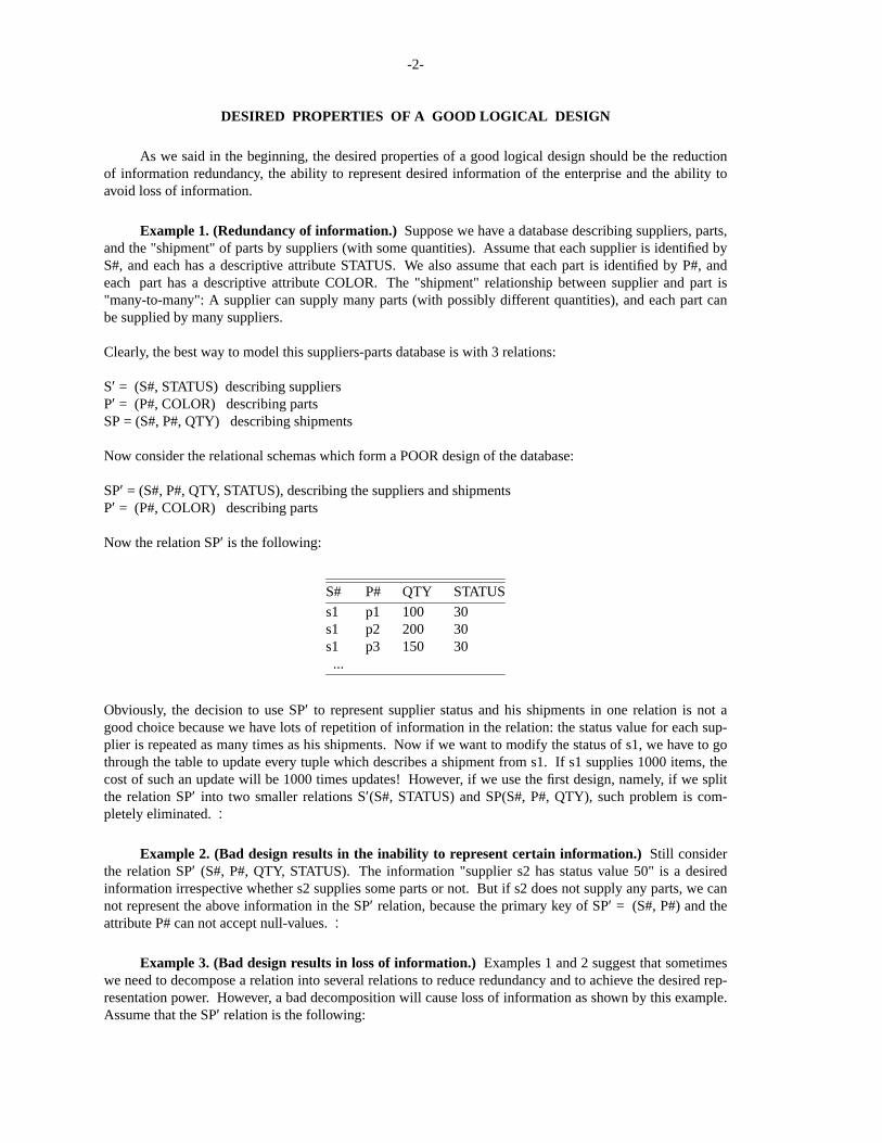
Now the relation SP′ is the following:

S# P# QTY STATUS

s1 p1 100 30s1 p2 200 30s1 p3 150 30...

Obviously, the decision to use SP′ to represent supplier status and his shipments in one relation is not agood choice because we have lots of repetition of information in the relation: the status value for each sup-plier is repeated as many times as his shipments. Now if we want to modify the status of s1, we have to gothrough the table to update every tuple which describes a shipment from s1. If s1 supplies 1000 items, thecost of such an update will be 1000 times updates! However, if we use the first design, namely, if we splitthe relation SP′ into two smaller relations S′(S#, STATUS) and SP(S#, P#, QTY), such problem is com-pletely eliminated. ♣

Example 2. (Bad design results in the inability to represent certain information.) Still considerthe relation SP′ (S#, P#, QTY, STATUS). The information "supplier s2 has status value 50" is a desiredinformation irrespective whether s2 supplies some parts or not. But if s2 does not supply any parts, we cannot represent the above information in the SP′ relation, because the primary key of SP′ = (S#, P#) and theattribute P# can not accept null-values. ♣

Example 3. (Bad design results in loss of information.) Examples 1 and 2 suggest that sometimeswe need to decompose a relation into several relations to reduce redundancy and to achieve the desired rep-resentation power. Howev er, a bad decomposition will cause loss of information as shown by this example.Assume that the SP′ relation is the following:

-3-

S# P# QTY STATUS

s1 p1 100 30s1 p2 200 30s2 p3 100 50

we decompose SP′ into SP′′ = (S#, P#, QTY) and S-Q = (QTY, STATUS):

Relation SP′′ Relation S-Q

S# P# QTY QTY STATUS

s1 p1 100 100 30s1 p2 200 200 30s2 p3 100 100 50

Now suppose that we want to get the information about the status of s1, using a natural join of SP′′ and S-Q. The resulting relation of the natural join becomes the following:

The relation obtained by joining SP′′ and S-Q

S# P# QTY STATUS

s1 p1 100 30s1 p1 100 50 (*)s1 p2 200 30s2 p3 100 30 (*)s2 p3 100 50

Note that we get 5 tuples instead of the original 3 in the relation SP′. Although we have more tuples, wehave less information, because we can no longer decide the status of s1 or s2 from the above relation, sim-ply due to the two spurious tuples (marked by (*)). So the desired information is lost as a result of baddesign. ♣

From the above examples, we can see that bad logical design can result in a database with lots ofredundancy and the scheme fails to represent the desired information. The solution to these problems is touse functional dependency as constraints and to apply the normalization technique in order to form the nor-malized relations which can avoid the problems of redundancy and loss of information.

-4-

FUNCTIONAL DEPENDENCY

Given a relation schema R(A1, ..., An), and X⊆R, Y ⊆R, we way R satisfies the functional dependency (fd)X → Y, i.e., X functionally determines Y, or Y is functionally determined by X, or Y is functionally depen-dent on X, if for each legal relation r(R) (i.e., r is a specific relation with attributes A1, ..., An), r satisfiesthe functional dependency X → Y.

A specific relation r satisfies X → Y if each X-value in r is associated with a unique Y-value in r. In otherwords, X functionally determines Y in a relation r if

for any two tuples t1 and t2 in r, if they hav e the same value on attribute X,then they also have the same value on attribute Y.

t1[X] = t2[X] ⇒ t1[Y] = t2[Y].

As an example of functional dependency, consider a relation schema R which has four attributesMOTHER, CHILD, GIFT, DATE, describing the mother’s gift-giving to her child on certain date. It is easyto see that each child has precisely one (biological) mother, while one mother can have sev eral children.That means if two tuples in r(R) hav e the same CHILD value (denoting the same child), they must have thesame MOTHER value (denoting the child’s mother). So we say that CHILD functionally determinesMOTHER or MOTHER is functionally determined by CHILD. Namely, CHILD → MOTHER. If we alsoassume that each child gets at most one gift on a fixed date, then we will also have the functional depen-dency (CHILD, DATE) → GIFT.(Think: What are the candidate keys of this relation schema R?)

An attribute Y of relation schema R is said to be fully functionally dependent on attribute X of R, if Yis functionally dependent on X but Y is not functionally dependent on any proper subset of X.

In the relation SP′(S#, P#, QTY, STATUS), the attribute STATUS is functionally dependent on theattribute (S#, P#), but it is not fully functionally dependent on (S#, P#) because STATUS is functionallydependent on S# which is a proper subset of the attribute (S#, P#).Think: in the above relation schema R(MOTHER, CHILD, GIFT, DATE) with functional dependencies F ={CHILD → MOTHER, (CHILD, DATE) → GIFT}, is the attribute MOTHER fully functionally dependenton (CHILD, DATE)?

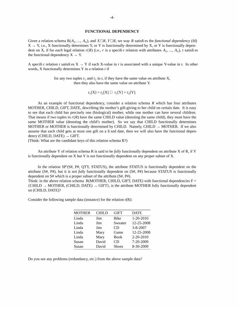
Consider the following sample data (instance) for the relation r(R):

MOTHER CHILD GIFT DATE

Linda Jim Bike 1-20-2010Linda Jim Sweater 12-25-2008Linda Jim CD 3-8-2007Linda Mary Game 12-25-2008Linda Mary Book 2-20-2010Susan David CD 7-20-2009Susan David Shoes 8-30-2009

Do you see any problems (redundancy, etc.) from the above sample data?

-5-

EXAMPLE OF FUNCTIONAL DEPENDENCY

The two most important things to remember about functional dependency (fd) are:

(1) Fd’s are determined by the meaning of the attributes andtheir role in the "real world" which is being modeled by the database.

(2) Fd’s are in turn used to group the attributes together to form thenormalized relations of the database.

Example. Consider the attributes

C Class (of a course)T Time for the classR Room for the classI Instructor of the class

which describe the arrangement of room and time for classes taught by the instructors. These attributes areused to model part of the "real world" in which we have classes at certain time in certain room lectured bycertain instructors. We hav e certain constraints about the objects (such as class, time, etc.) in the "realworld" and such constraints are in turn represented in terms of functional dependencies. The constraintsare:

(1) No two instructors teach the same course.

(2) At any time and in a given room, there is at most one class being taught there.

(3) No class can be taught at one given time in two rooms.

(4) No instructor can teach two classes at one given time.

-6-

The functional dependencies are:

(a) C → I(b) TR → C(c) CT → R(d) IT → C

Given below is a database which has some tuples violating the above functional dependencies.

Class Instructor Time Room

Csc4402 Chen 1:30/M 101His7700 Brown 3:00/T 205

Csc4402 Smith 2:00/F 310 (a)Art2450 John 3:00/T 205 (b)His7700 Brown 3:00/T 208 (c)Csc7420 Chen 1:30/M 202 (d)

It is easy to see that the tuples marked (a), (b), (c), (d) violate the functional dependencies (a), (b), (c), (d)respectively.

-7-

AXIOMS FOR FUNCTIONAL DEPENDENCIES

Logical implications of dependencies. Let R(ABC) be a relation schema and F = {A → B, B → C}be the set of functional dependencies that hold on R. It is easy to see that the fd A → C also holds in R.

In general, let F be a set of functional dependencies and let X → Y be a functional dependency. Wesay F logically implies X → Y, written F |= X → Y, if every relation instance r that satisfies F also satisfiesX → Y.

The closure of F

The closure of F, denoted as F+, is defined as the set of all the functional dependencies that are logi-cally implied by F. That is, F+ ={X → Y | F |= X → Y}.

Axioms for Functional Dependencies

To determine candidate keys, and to understand logical implications among functional dependencies,we need to compute F+, or at least, to tell, for given F and fd X → Y, whether X → Y is in F+. So weneed inference rules to tell us how one or more fd’s imply other fd’s. The set of rules is called Armstrong’saxioms, or Armstrong’s rules. These rules are both sound and complete.

(1). The soundness of the rules refers to the fact that using the rules, we can not deduce from F any fd’swhich are not in F+.

(2). The completeness of the Armstrong’s rules refers to the fact that given a set of functional dependen-cies F, we can deduce all the dependencies in F+ from F using these rules.

Let F* = F ∪ { X → Y | X → Y is deduced from F using the Armstrong’s rules}. Here F* is the setof functional dependencies derivable from F using the Armstrong’s rules. The soundness of the Arm-strong’s rules tells us F* ⊆ F+ and the completeness of the rules indicates F+ ⊆ F*. Together, wehave F+ = F*. In other words, an fd X → Y belongs to F+ if and only if X → Y can be deducedfrom F by using the Armstrong’s rules.

Now we can define F+ in terms of F and Armstrong’s rules. The closure F+ of F is the set of all fd’swhich can be derived using the rules (1) - (3) (in next page) starting with the fd’s in F, and including thosein F.

-8-

ARMSTRONG’S RULES

In the example relation R(ABC) given earlier, we noticed that from the following functional depen-dencies {A → B , B → C}, we can deduce A → C by transitivity, and deduce AB → C by a simple applica-tion of the definition of functional dependency. In fact, using the following Armstrong’s rules, we candeduce AB → C from either A → C or B → C.

Armstrong’s rules:

(1) X → X′ for all subsets X′ ⊆ X (projection rule)(2) if X → Y then XZ → YZ (augmentation rule)(3) if X → Y and Y → Z then X → Z (transitive rule)

We can also derive many other rules by repeated application of the rules (1) - (3). For example, wecan obtain the union rule:

if X → Y and X → Z then X → YZ.

X → Y giv es X → XY by (2)X → Z giv es XY → YZ by (2)X → XY andXY → YZ gives X → YZ by (3)

Also, we can derive the decomposition rule:

if X → YZ then X → Y and X → Z.

YZ → Y by (1)YZ → Z by (1)

X → YZ andYZ → Y giv es X → Y by (3)X → YZ andYZ → Z giv es X → Z by (3)

The importance of the Armstrong’s rules lies in that they allow manipulation of the fd’s purely in asyntactic way without looking at the tuples of a relation.

-9-

DETERMINING DEPENDENT ATTRIBUTES

Let X be a set of attributes and F be a set of functional dependencies. Let X+ be the set of all attributes thatdepend on a subset of X with respect to F, i.e., X+ is the set of attributes Z, such that X → Z ∈ F+. X+ iscalled the closure of X (w.r.t. F). By definition, X ⊆ X+.

The algorithm for computing X+ (w.r.t. F):

Input: A relation schema R, a set of functional dependencies F and a set of attributes X.Output: X+.

(1) X+ ← X.(2) Repeat

found ← false;for (each fd Y → Z ∈ F) do

if (Y ⊆ X+)then begin

found ← true;X+ ← X+ ∪ Z;remove Y → Z from further consideration;end;

until (found = false) or (X+ = all attributes).

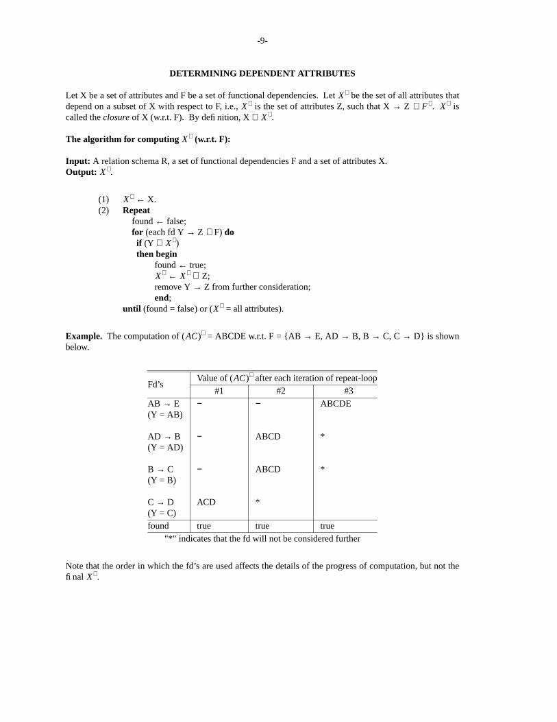
Example. The computation of (AC)+ = ABCDE w.r.t. F = {AB → E, AD → B, B → C, C → D} is shownbelow.

Value of (AC)+ after each iteration of repeat-loop

#1 #2 #3Fd’s

AB → E − − ABCDE(Y = AB)

AD → B − ABCD *(Y = AD)

B → C − ABCD *(Y = B)

C → D ACD *(Y = C)

found true true true

"*" indicates that the fd will not be considered further

Note that the order in which the fd’s are used affects the details of the progress of computation, but not thefinal X+.

-10-

Example - Compact Representation of F+. If F = {AB → C, C → B, C → A}, then we can use thefollowing functional dependencies as a shorthand to represent F+: (The right hand side of each fd is simplythe X+ where X = the left hand side; the X’s are all the non-empty subsets of the attributes (ABC)).

A → AB → BC → ABCAB → ABCAC → ABCBC → ABCABC → ABC

Note that we do not mean that the F+ consists of only the above 7 functional dependencies. In fact,each X → Y in the above represents the set of all the fd’s in the form of X → Z, where Z is a subset of Y.For example, the fd AC → ABC represents the set of fd’s {AC → A, AC → B, AC → C, AC → AB, AC →AC, AC → BC, AC → ABC}. The reason that we represent F+ only with the above 7 functional dependen-cies is for the sake of clarity and conciseness.

-11-

EQUIVALENCE AND REDUNDANCY OF FD’S

Tw o sets of fd’s F1 and F2 are said to be equivalent, F1 ≡ F2, if they hav e the same closure:

F+1 = F+

2 ,

or equivalently,

F1 ⊆ F+2 and F2 ⊆ F+

1 .

Note that to test F1 ⊆ F+2 , we need not compute all of F+

2 . We need only to verify that for each X → Y ∈F1, we hav e X → Y ∈ F+

2 , i.e., the closure X+ computed using F2 contains Y.

Example. Let F1 = {A → B, B → C, C → A} and F2 = {A → C, C → B, B → A}. Then F1 ≡ F2.

This is true because A+ using F2 equals ABC which contains B. Thus A → B ∈ F+2 . Similarly, B → C and

C → A are in F+2 , etc.

Redundant fd. An fd f ∈ F is redundant if F ≡ F − {f}.

Example. A → C is redundant in {A → B, B → C, A → C}.

Theorem. F1 ≡ F2 if and only if for each subset of attributes X, X+1 = X+

2 , where X+i is the closure of

X computed using the fd’s in Fi .

Theorem. An fd X → Y in F is redundant if and only if Y ⊆ X+, where X+ is computed withoutusing the fd X → Y.

A set of fd’s is said to be reduced if it contains no redundant fd’s.

Example. The set F = {A → B, B → C, C → A, A → C, C → B, B → A} can be reduced in twoways by successively removing the redundant fd’s.

1. {A → B, B → C, C → A}

2. {A → C, C → B, B → A}

Note that removing a redundant fd from a set F does not affect the closure F+. There are some other waysto reduce the set F, you may try to find them.

-12-

MINIMAL COVERS

Let F1 and F2 be two sets of functional dependencies. If F1 ≡ F2, then we say the F1 is a cover ofF2 and F2 is a cover of F1. We also say that F1 covers F2 and vice versa. It is easy to show that every setof functional dependencies F is covered by a set of functional dependencies G, in which the right hand sideof each fd has only one attribute.

We say a set of dependencies F is minimal if:

(1) Every right hand side of each fd in F is a single attribute.

(2) The left hand side of each fd does not have any redundant attribute, i.e., for every fd X → A in Fwhere X is a composite attribute, and for any proper subset Z of X, the functional dependency Z → A∉ F+.

(3) F is reduced (without redundant fd’s). This means that for every X → A in F, the set F − {X → A} isNOT equivalent to F.

Minimal Covers of F. It is easy to see that for each set F of functional dependencies, there exists aset of functional dependencies F′ such that F ≡ F′ and F′ is minimal. We call such F′ a minimal cover of F.

The algorithm to compute F′, a minimal cover of F.

Input: F, a set of fd’s.output: F′, a minimal cover of F.

(1) Let F′ = {X → A | X → A ∈ F and A is a single attribute}. For each fd X → A1 A2 ... An ∈ F (n > 1),put the fd’s X → A1, X → A2, ..., X → An into F′, where Ai is a single attribute.

(2) Whilethere is an fd X → A ∈ F′ such that X is a composite attribute and Z ⊂ X is a proper subset ofX and Z → A ∈ (F ′)+,

doreplace X → A with Z → A.

(3) For each fd X → A ∈ F′, check if it is redundant, if it is, eliminate it. ♣

It is important to note that for the above algorithm, the ordering between step (2) and step (3) is criti-cal: If you first perform step (3) and then perform step (2) of the algorithm, the resulting set of fd’s may stillhave redundant functional dependencies.

It should be pointed out that for a set of functional dependencies F, there may be more than one mini-mal covers of F.

-13-

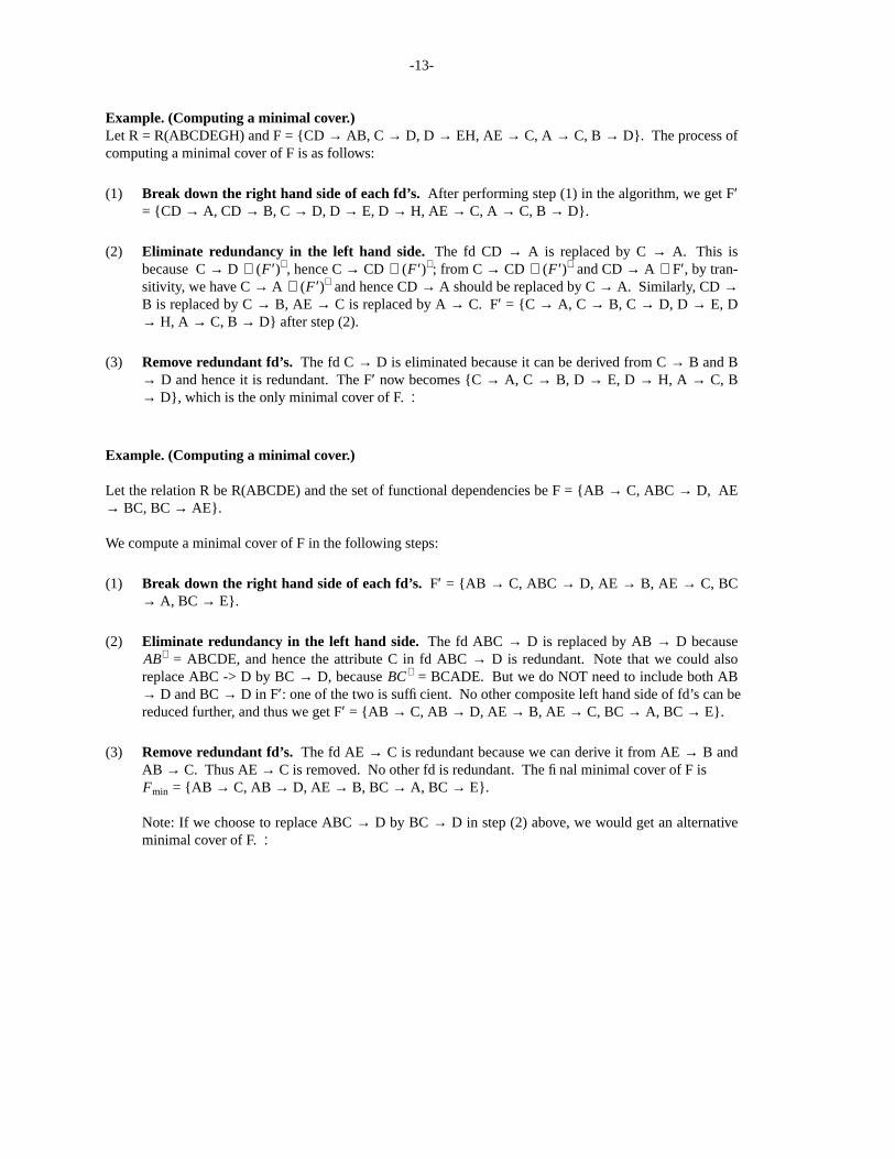
Example. (Computing a minimal cover.)Let R = R(ABCDEGH) and F = {CD → AB, C → D, D → EH, AE → C, A → C, B → D}. The process ofcomputing a minimal cover of F is as follows:

(1) Break down the right hand side of each fd’s. After performing step (1) in the algorithm, we get F′= {CD → A, CD → B, C → D, D → E, D → H, AE → C, A → C, B → D}.

(2) Eliminate redundancy in the left hand side. The fd CD → A is replaced by C → A. This isbecause C → D ∈ (F ′)+, hence C → CD ∈ (F ′)+; from C → CD ∈ (F ′)+ and CD → A ∈ F′, by tran-sitivity, we hav e C → A ∈ (F ′)+ and hence CD → A should be replaced by C → A. Similarly, CD →B is replaced by C → B, AE → C is replaced by A → C. F′ = {C → A, C → B, C → D, D → E, D→ H, A → C, B → D} after step (2).

(3) Remove redundant fd’s. The fd C → D is eliminated because it can be derived from C → B and B→ D and hence it is redundant. The F′ now becomes {C → A, C → B, D → E, D → H, A → C, B→ D}, which is the only minimal cover of F. ♣

Example. (Computing a minimal cover.)

Let the relation R be R(ABCDE) and the set of functional dependencies be F = {AB → C, ABC → D, AE→ BC, BC → AE}.

We compute a minimal cover of F in the following steps:

(1) Break down the right hand side of each fd’s. F′ = {AB → C, ABC → D, AE → B, AE → C, BC→ A, BC → E}.

(2) Eliminate redundancy in the left hand side. The fd ABC → D is replaced by AB → D becauseAB+ = ABCDE, and hence the attribute C in fd ABC → D is redundant. Note that we could alsoreplace ABC -> D by BC → D, because BC+ = BCADE. But we do NOT need to include both AB→ D and BC → D in F′: one of the two is sufficient. No other composite left hand side of fd’s can bereduced further, and thus we get F′ = {AB → C, AB → D, AE → B, AE → C, BC → A, BC → E}.

(3) Remove redundant fd’s. The fd AE → C is redundant because we can derive it from AE → B andAB → C. Thus AE → C is removed. No other fd is redundant. The final minimal cover of F isFmin = {AB → C, AB → D, AE → B, BC → A, BC → E}.

Note: If we choose to replace ABC → D by BC → D in step (2) above, we would get an alternativeminimal cover of F. ♣

-14-

CANDIDATE KEYS

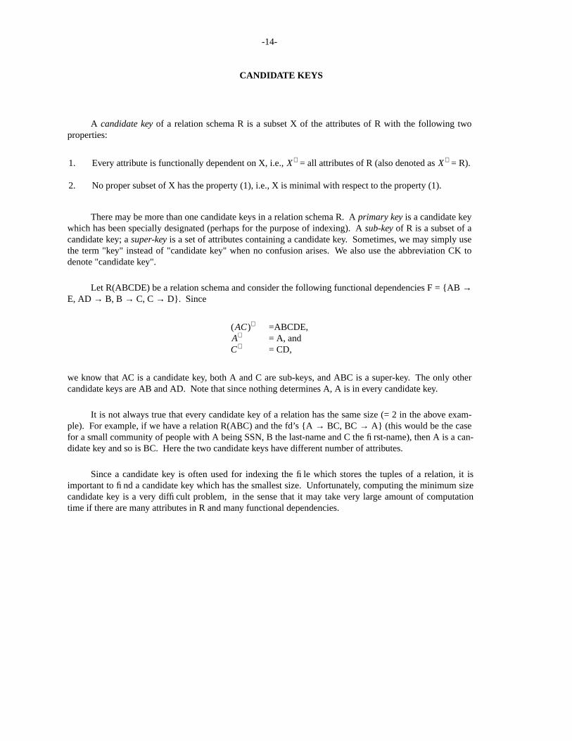
A candidate key of a relation schema R is a subset X of the attributes of R with the following twoproperties:

1. Every attribute is functionally dependent on X, i.e., X+ = all attributes of R (also denoted as X+ = R).

2. No proper subset of X has the property (1), i.e., X is minimal with respect to the property (1).

There may be more than one candidate keys in a relation schema R. A primary key is a candidate keywhich has been specially designated (perhaps for the purpose of indexing). A sub-key of R is a subset of acandidate key; a super-key is a set of attributes containing a candidate key. Sometimes, we may simply usethe term "key" instead of "candidate key" when no confusion arises. We also use the abbreviation CK todenote "candidate key".

Let R(ABCDE) be a relation schema and consider the following functional dependencies F = {AB →E, AD → B, B → C, C → D}. Since

(AC)+ =ABCDE,A+ = A, andC+ = CD,

we know that AC is a candidate key, both A and C are sub-keys, and ABC is a super-key. The only othercandidate keys are AB and AD. Note that since nothing determines A, A is in every candidate key.

It is not always true that every candidate key of a relation has the same size (= 2 in the above exam-ple). For example, if we have a relation R(ABC) and the fd’s {A → BC, BC → A} (this would be the casefor a small community of people with A being SSN, B the last-name and C the first-name), then A is a can-didate key and so is BC. Here the two candidate keys hav e different number of attributes.

Since a candidate key is often used for indexing the file which stores the tuples of a relation, it isimportant to find a candidate key which has the smallest size. Unfortunately, computing the minimum sizecandidate key is a very difficult problem, in the sense that it may take very large amount of computationtime if there are many attributes in R and many functional dependencies.

-15-

General Idea of the Algorithm for Computing All Candidate Keys of a Relation.

Given a relation R(A1, A2, ..., An) and a set of functional dependencies F which are true on R, how can wecompute all candidate keys of R?

Since each candidate key must be a minimal subset of {A1, ..., An} which determines all attributes of R, themost straightforward (and brute-force) way to compute all candidate keys of R is the following:

(1) Construct a list L consisting of all non-empty subsets of {A1, ..., An} (there are 2n − 1 of them).These subsets are arranged in L in ascending order of the size of the subset: We get L = ⟨ Z1, Z2, ...,Z2n−1⟩, such that |Zi | ≤ |Zi+1|. Here |Zi | denotes the number of elements in the set Zi .

(2) Initialize the set K = {} (K will contain all CK’s of R).While L is not empty, remove the first element Zi from L, and compute Zi

+.If Zi

+ = R, then

(a) Add Zi to K

(b) Remove any element Z j from L if Zi ⊂ Z j (because Z j is too big, it can not be a CK).

(3) Output K as the final result.

-16-

General Idea of the Algorithm for Computing All Candidate Keys of a Relation - Continued.

Analysis: The method in previous page is correct but not efficient: the list L is too big (exponential in thenumber of attributes in R). Thus we need to utilize some "clever" ideas to cut down the number of Zi’s thatthe algorithm has to check. The general idea of the CK computing algorithm is to focus on only attributesthat will definitely appear in ANY candidate key of R, and ignore any attribute that will NEVER be part ofa CK. The following notions are useful for this purpose:

Necessary attributes:An attribute A is said to be a necessary attribute if

(a) A occurs only in the L.H.S. (left hand side) of the fd’s in F; or

(b) A is an attribute in relation R, but A does not occur in either L.H.S. or R.H.S. of any fd in F.

In other words, necessary attributes NEVER occur in the R.H.S. of any fd in F.

Useless attributes:An attribute A is a useless attribute if A occurs ONLY in the R.H.S. of fd’s in F.

Middle-ground attributes:An attribute A in relation R is a middle-ground attribute if A is neither necessary nor useless.

Example.Consider the relation R(ABCDEG) with set of fd’s F = {AB → C, C → D, AD → E}

All attributes of R are partitioned as follows:

Necessary Useless Middle-ground

A, B, G E C, D

An important observation about necessary attribute is: a necessary attribute will appear in every CKof R, and thus ALL necessary attributes must appear in every CK of R. Thus, if X is the collection of ALLnecessary attributes (and thus X can be seen as a composite attribute), and X+ = All attributes of R, then Xmust be the ONLY candidate key of R. (Think: Why is that?)

Thus we should first check the necessary attribute closure X+, and terminate the CK computing algorithmwhen X+ = R. On the other hand, we also notice that useless attributes can never be part of any CK. There-fore, in case X+ ≠ R, and we have to enumerate subsets Zi of R to find CK’s, the Zi’s should NOT containany useless attributes, and each Zi should contain all the necessary attributes. In fact, the list L of subsetsto test should be constructed from all non-empty subsets of the middle-ground attributes, with each subsetexpanded to include all necessary attributes.

-17-

The algorithm for computing all candidate keys of R.

Input: A relation R={ A1, A2, ..., An}, and F, a set of functional dependencies.Output: K={ K1, . . . , Kt}, the set of all candidate keys of R.

Step1.Set F′ to a minimal cover of F (This is needed because otherwise we may not detect all uselessattributes).

Step2.Partition all attributes in R into necessary, useless and middle-ground attribute sets accordingto F′. Let X={ C1, . . . , Cl} be the necessary attribute set, Y = {B1, ..., Bk} be the uselessattribute set, and M = {A1, ..., An} − (X ∪ Y) be the middle-ground attribute set.If X={}, then go to step4.

Step3.Compute X+. If X+ =R, then set K= {X}, terminate.

Step4.Let L = ⟨Z1, Z2, . . . , Zm⟩ be the list of all non-empty subsets of M (the middle-groundattributes) such that L is arranged in ascending order of the size of Zi .Add all attributes in X (necessary attributes) to each Zi in L.

Set K = {}.i ← 0.

WHILE L ≠ empty doBEGIN

i ← i + 1.Remove the first element Z from L.Compute Z+.If Z+ = R,thenbegin

set K ← K ∪ {Z};for any Z j ∈ L, if Z ⊂ Z j

then L ← L − {Z j}.end

END♣

-18-

Example. (Computing all candidate keys of R.)Let R = R(ABCDEG) and F = {AB → CD, A → B, B → C, C → E, BD → A}. The process to compute allcandidate keys of R is as follows:

(1) The minimal cover of F is {A → B, A → D, B → C, C → E, BD → A}.

(2) Since attribute G never appears in any fd’s in the set of functional dependencies, G must beincluded in a candidate key of R. The attribute E appears only in the right hand side of fd’s andhence E is not in any key of R. No attribute of R appears only in the left hand side of the set offd’s. Therefore X = G at the end of step 2.

(3) Compute G+ = G, so G is not a candidate key.

(4) The following table shows the L, K, Z and Z+ at the very beginning of each iteration in theWHILE statement.

i Z Z+ L K

⟨AG, BG, CG, DG, ABG, ACG, ADG, BCG,BDG, CDG, ABCG, ABDG, ACDG, BCDG, ABCDG⟩0 − − {}

1 AG ABCDEG = R ⟨BG, CG, DG, BCG, BDG, CDG, BCDG⟩ {AG}

2 BG BCEG ≠ R ⟨CG, DG, BCG, BDG, CDG, BCDG⟩ {AG}

3 CG CEG ≠ R ⟨DG, BCG, BDG, CDG, BCDG⟩ {AG}

4 DG DG ≠ R ⟨BCG, BDG, CDG, BCDG⟩ {AG}

5 BCG BCEG ≠ R ⟨BDG, CDG, BCDG⟩ {AG}

6 BDG ABCDEG = R ⟨CDG⟩ {AG, BDG}

7 CDG CEDG ≠ R ⟨ ⟩ {AG, BDG}

-19-

FIRST, SECOND NORMAL FORM

First normal form. A relation R is said to be in first normal form if all the underlyingdomains of R contain only atomic values. It is easy to see that if R is in first normal form, then Rdoes not contain any repeating groups. We write 1NF as a short hand for first normal form.

Non-key attribute. An attribute A in relation R is said to be a non-key attribute if it is not asubkey, i.e., A is not a component of any candidate key K of R.

Second normal form. A relation R is said to be in second normal form if R is in 1NF andev ery non-key attribute is fully dependent on each candidate key K of R. In Example 1, the relationSP′ has only one candidate key (S#, P#). The attribute STATUS is a non-key attribute of SP′ and it isnot fully dependent on (S#, P#), therefore SP′ is not in 2NF.

Although relations in 2NF have better properties than those in 1NF, there are still problemswith them. These problems motivate the search for more "ideal" form of relations and hence the 3NFand BCNF normal forms are identified. In general, in the logical design process, we may start with arelation which is in 1NF (or even it is not in 1NF so we have to first transform it into 1NF), then usethe functional dependencies as constraints to decompose R into several relations R1, ..., Rk such thateach Ri is in 3NF (or even better, in BCNF) and the natural join of R1, ..., Rk gives the same informa-tion as contained in R.

-20-

LOSS-LESS-JOIN DECOMPOSITION

The decomposition

(S#, P#, QTY, STATUS) = (S#, P#, QTY) ⊗ (S#, STATUS)

is called a loss-less-join (LLJ) decomposition, or we say that the decomposition is loss-less, becausethe join of the component relations (S#, P#, QTY) and (S#, STATUS) gives back the original relation(S#, P#, QTY, STATUS).

Notice that the resulting relations R1 = (S#, P#, QTY) and R2 = (S#, STATUS) have betterproperties than the original relation SP′ = (S#, P#, QTY, STATUS). For example, assume that wehave only one shipment from supplier s3 which is "s3, p4, 100, 60" in SP′. Now we delete this tuplefrom SP′ because s3 stops supplying p4. Then the information "the status of s3 is 60" will be gonefrom relation SP′, while in the case of R1 and R2, we delete the tuple "s3, p4, 100" from R1 but thetuple "s3, 60" remains to be in R2.

We must be very careful in performing the decomposition otherwise the loss-less property maynot be maintained. As we have seen in Example 3, if we decompose SP′ into (S#, P#, QTY) and(QTY, STATUS), the loss-less property is gone because the join of the latter two relations createsome spurious tuples. Intuitively, the decomposition of SP′ = R1 ⊗ R2 is loss-less because theattribute "S#" which is mutual to R1 and R2 can uniquely determine the attribute "STATUS", but themutual attribute "QTY" in the second decomposition can not determine "STATUS". Theoretically,we have the following theorem which tells us the sufficient condition for a decomposition to be loss-less.

Heath Theorem. For a relation R with attributes A, B, C and functional dependency A → B,the decomposition

R(A, B, C) = R1(A, B) ⊗ R2(A, C)

is always loss-less.

The two most desirable properties of any decomposition of a relation R are:

(1) loss-less, and(2) fd-preserving.

Let R be a relation schema with functional dependencies F. Assume that we have a decompo-sition of R into a set of relations R1, R2, ..., Rk , and the F is subsequently decomposed into F1, F2,..., Fk . As we already discussed before, we want the decomposition to be "loss-less" in the sense thatthe natural join of the R1, R2, ..., Rk is exactly R, i.e., R = R1 ⊗ R2 ⊗ ... ⊗ Rk . Another desirableproperty of a decomposition is functional dependency-preserving (fd-preserving), i.e., we want tomaintain all the functional dependencies by requiring F1 ∪ F2 ∪ ... ∪ Fk ≡ F.

-21-

THIRD NORMAL FORM AND 3NF DECOMPOSITION

A relation schema R with a set fd’s F is said to be in third normal form (3NF) if for each fd X→ A ∈ F (here A is a single attribute), we have

either X is a superkey

or A is a prime.

An attribute A is called a prime if A is a subkey, i.e., A is a component of a key.

Example. The relation (ADB) with F = {AD → B, B → D} is in 3NF, because AD and ABare its keys, and thus although B in B → D is not a superkey, D is a prime.

As we can see clearly, the 3NF requirement is weaker than the BCNF. As a result, we canalways find a 3NF decomposition of a relation R such that the decomposition is both LLJ and fd-pre-serving.

Bernstein’s Theorem. Every relation has a loss-less, fd-preserving 3NF decomposition.

-22-

BERNSTEIN’S ALGORITHM

Input: A set of attributes in R and a set F of functional dependencies in R (assume F is already minimal).

Output: A set of 3NF relations that form a loss-less, fd-preserving decomposition of R.

Algorithm:

1. Group together all fd’s which have the same L.H.S. If X → Y1,X → Y2, ..., X → Yk are all the fd’s with the L.H.S. X, then replaceall of them by the single fd X →Y1Y2 ... Yk .

2. For each fd X → Y in F, form the relation (XY) in the decomposition.

3. IF X′Y′ ⊂ XY, then remove the relation (X′Y′) from the decomposition.

4. If none of the relations in the decomposition contains a candidate key ofthe original relation, then find a candidate key K of R and add the relation (K)to the decomposition.

Example. This example shows the need for step 1 and 3. Let attributes = ABC and F = {A → B, A→ C, C → A}.

Step 1. {A → BC, C → A}.Step 2. (ABC), (CA)Step 3. (ABC)Step 4. (ABC); the key A is contained in ABC.

The decomposition (ABC) = (AB) ⊗ (AC) is not preferred because it causes unnecessaryduplication of values for the attribute A. The relation R(ABC) is already in 3NF.

A B C A B A C

a1 b1 c1 a1 b1 a1 c1a2 b1 c2 = a2 b1 ⊗ a2 c2a3 b3 c3 a3 b3 a3 c3

-23-

BOYCE-CODD NORMAL FORM (BCNF)

A relation schema R is in BCNF, if for every nontrivial functional dependency X → Y thatholds on R, the attribute X is a superkey.

We often want to decompose a relation R which is not in BCNF into a set of smaller relationsR1, R2, ..., Rn such that each Ri is in BCNF. Such a decomposition of R is called a BCNF decompo-sition of the relation R.

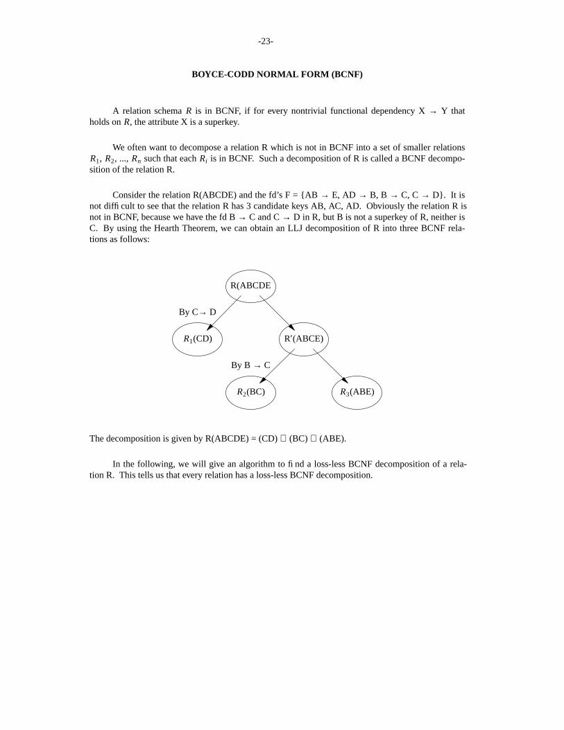
Consider the relation R(ABCDE) and the fd’s F = {AB → E, AD → B, B → C, C → D}. It isnot difficult to see that the relation R has 3 candidate keys AB, AC, AD. Obviously the relation R isnot in BCNF, because we have the fd B → C and C → D in R, but B is not a superkey of R, neither isC. By using the Hearth Theorem, we can obtain an LLJ decomposition of R into three BCNF rela-tions as follows:

R(ABCDE

R1(CD) R′(ABCE)

By C→ D

R2(BC) R3(ABE)

By B → C

The decomposition is given by R(ABCDE) = (CD) ⊗ (BC) ⊗ (ABE).

In the following, we will give an algorithm to find a loss-less BCNF decomposition of a rela-tion R. This tells us that every relation has a loss-less BCNF decomposition.

-24-

Algorithm to decompose a relation R into a set of BCNF relations

Input: Relation R and set of functional dependencies F (F is minimal)Output: Result={ R1, R2, ..., Rn } such that(A) Each Ri is in BCNF(B) The decomposition is loss-less-join decomposition

1. Group together all fd’s which have the same L.H.S. If X → Y1, X → Y2 , . . . , X → Yk are inF, then replace all of them by a single fd X → Y , where Y=Y1 Y2

. . . Yk .result := {R};done := FALSE;Compute F+; // Using the compact representation discussed in page 10

2. WHILE (NOT done) DOIF (there is a scheme Ri in result that is not in BCNF)THEN BEGIN

Let X→Y be a nontrivial functional dependency in F+ that holds on Ri

such that X→ Ri is not in F+;result :=(result − {Ri} ) ∪ {(Ri − Y), (XY)};(this means to break Ri into two relations Ri − Y and XY)

ENDELSE done := TRUE ;

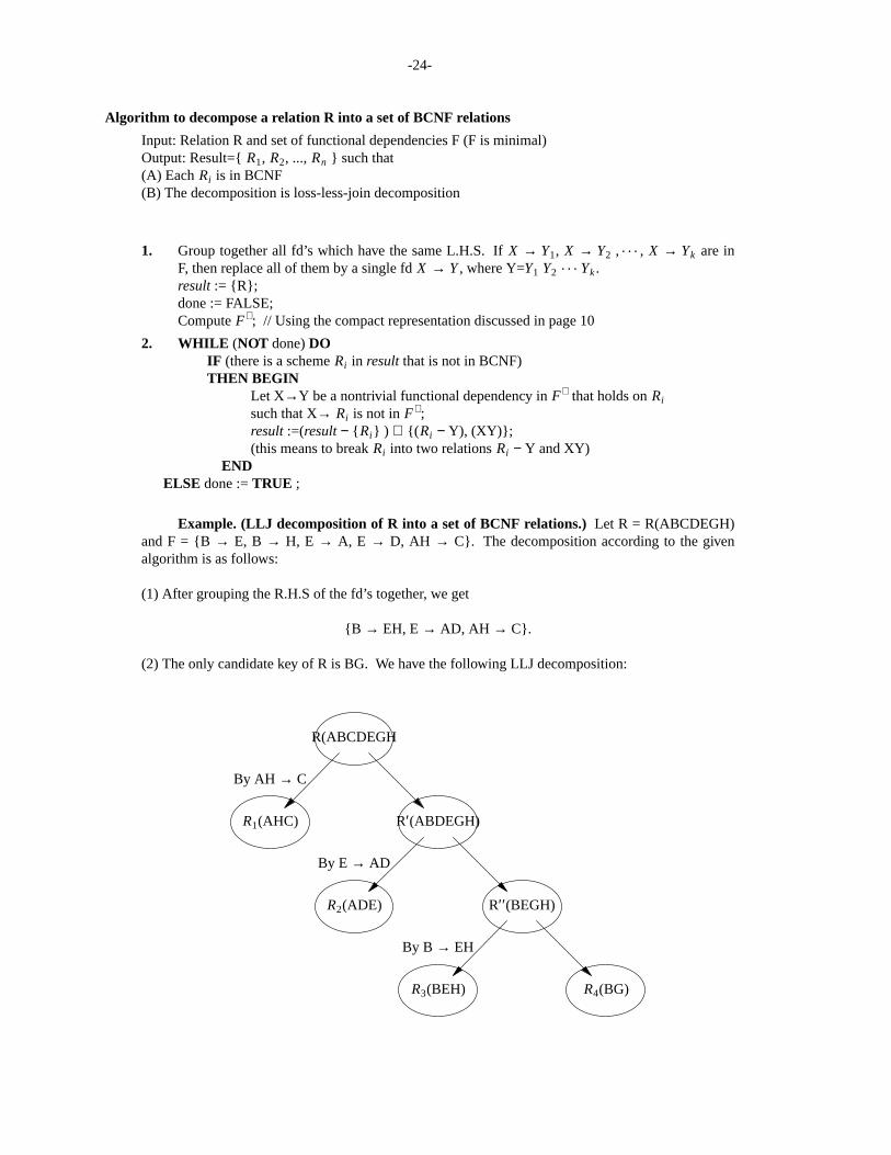
Example. (LLJ decomposition of R into a set of BCNF relations.) Let R = R(ABCDEGH)and F = {B → E, B → H, E → A, E → D, AH → C}. The decomposition according to the givenalgorithm is as follows:

(1) After grouping the R.H.S of the fd’s together, we get

{B → EH, E → AD, AH → C}.

(2) The only candidate key of R is BG. We hav e the following LLJ decomposition:

R(ABCDEGH

R1(AHC) R′(ABDEGH)

By AH → C

R2(ADE) R′′(BEGH)

R3(BEH) R4(BG)

By E → AD

By B → EH

-25-

It is easy to verify that the four resulting relations are all in BCNF, and

R(ABCDEHG) = (AHC) ⊗ (EAD) ⊗ (BEH) ⊗ (BG).

Also we can see that all the functional dependencies in F are preserved.