Lecture Notes #7: Residual Analysis and Multiple ...gonzo/coursenotes/file7.pdfmore examples of this...

Lecture Notes #7: Residual Analysis and Multiple Regression 7-1

Richard GonzalezPsych 613Version 2.5 (Dec 2016)

LECTURE NOTES #7: Residual Analysis and Multiple Regression

Reading Assignment

KNNL chapter 6 and chapter 10; CCWA chapters 4, 8, and 10

1. Statistical assumptions

The standard regression model assumes that the residuals, or ε’s, are independently,identically distributed (usually called“iid”for short) as normal with µ = 0 and varianceσ2.

(a) Independence

A residual should not be related to another residual. Situations where indepen-dence could be violated include repeated measures and time series because twoor more residuals come from the same subject and hence may be correlated. An-other violation of independence comes from nested designs where subjects areclustered (such as in the same school, same family, same neighborhood). Thereare regression techniques that relax the independence assumption, as we saw inthe repeated measures section of the course.

(b) Identically distributed

As stated above, we assume that the residuals are distributed N(0, σ2ε ). Thatis, we assume that each residual is sampled from the same normal distributionwith a mean of zero and the same variance throughout. This is identical tothe normality and equality of variance assumptions we had in the ANOVA. Theterminology applies to regression in a slightly different manner, i.e., defined asconstant variance along the entire range of the predictor variable, but the ideais the same.

The MSE from the regression source table provides an estimate of the varianceσ2ε for the ε’s.

Usually, we don’t have enough data at any given level of X to check whetherthe Y’s are normally distributed with constant variance, so how should this


assumption be checked? One may plot the residuals against the predicted scores(or instead the predictor variable). There should be no apparent pattern in theresidual plot. However, if there is fanning in (or fanning out), then the equalityof variance part of this assumption may be violated.

To check the normality part of the assumption, look at the histogram of theresiduals to see whether it resembles a symmetric bell-shaped curve. Better still,look at the normal probability plot of the residuals (recall the discussion of thisplot from the ANOVA lectures).

2. Below I list six problems and discuss how to deal with each of them (see Ch. 3 ofKNNL for more detail)

(a) The association is not linear. You check this by looking at the scatter plot ofX and Y. If you see anything that doesn’t look like a straight line, then youshouldn’t run a linear regression. You can either transform or use a model thatallows curvature such as polynomial regression or nonlinear regression, which wewill discuss later. Plotting residuals against the predicted scores will also helpdetect nonlinearity.

(b) Error terms do not have constant variance. This can be observed in the residualplots. You can detect this by plotting the residuals against the predictor variable.The residual plot should have near constant variance along the levels of thepredictor; there should be no systematic pattern. The plot should look like ahorizontal band of points.

(c) The error terms are not independent. We can infer the appropriateness of this as-sumption from the details of study design, such as if there are repeated measuresvariables. You can perform a scatter plot of residuals against time to see if thereis a pattern (there shouldn’t be a correlation). Other sources of independenceviolations are due to grouping such as data from multiple family members ormultiple students from the same classroom; there may be correlations betweenindividuals in the same family or individuals in the same classroom.

(d) Outliers. There are many ways to check for outliers (scatter plot of Y andX, examining the numerical value of the residuals, plotting residuals against thepredictor). We’ll also cover a more quantitative method of determining the degreeto which an outlier influences the regression line.

(e) Residuals are not normally distributed. This is checked by either looking at thehistogram of the residuals or the normal-normal plot of the residuals.


(f) You have the wrong structural model (aka a mispecified model). You can also useresiduals to check whether an additional variable should be added to a regressionequation. For example, if you run a regression with two predictors, you can takethe residuals from that regression and plot them against other variables thatare available. If you see any systematic pattern other than a horizontal band,then that is a signal that there may be useful information in that new variable(i.e., information not already accounted for by the linear combination of the twopredictors already in the regression equation that produced those residuals).

3. Nonlinearity

What do you do if the scatterplot of the raw data, or the scatterplot of the residu-als against the predicted scores, suggests that the association between the criterionvariable Y and the predictor variable X is nonlinear? One possibility is that youcan re-specify the model. Rather than having a simple linear model of the form Y= β0 + β1X, you could add more predictors. Perhaps a polynomial of the form Y= β0 + β1X + β2X

2 would be a better fit. Along similar lines, you may be able totransform one of the variables to convert the model into a linear model. Either way(adding predictors or transforming existing predictors) we have an exciting challengein regression because you are trying to find a model that fits the data. Through theprocess of finding such a model, you might learn something about theory or the psy-chological processes underlying your phenomenon. There could be useful informationin the nature of the curvature (processes that speed up or slow down at particularcritical points).

There are sensible ways of diagnosing how models are going wrong and how to improvea model. You could examine residuals. If a linear relation holds, then there won’t bemuch pattern in the residuals. To the degree there is a relation in the residuals whenplotted against a predictor variable, then that is a clue that the model is misspecified.

4. The “Rule of the Bulge” to decide on transformations.

Here is a heuristic for finding power transformations to linearize data. It’s basically amnemonic for remembering which transformation applies in which situation, much likethe mnemonics that help you remember the order of the planets (e.g., My Very Edu-cated Mother Just Saved Us Nine Pies; though recent debate now questions whetherthe last of those pies should be saved. . . ). A more statistics-related mnemonic canhelp you remember the three key statistical assumptions. INCA: independent normalconstant-variance assumptions (Hunt, 2010, Teaching Statistics, 32, 73-74).

The rule operates within the power family of transformations xp. Recall that withinthe power family, the identity transformation (i.e., no transformation) corresponds to


p = 1. Taking p = 1 as the reference point, we can talk about either increasing p(say, making it 2 or 3) or decreasing p (say, making it 0, which leads to the log, or -1,which is the reciprocal).

With two variables Y and X it is possible to transform either variable. That is, eitherof these are possible: Yp = β0 + β1 X or Y = β0 + β1 Xp. Of course, the twoexponents in these equations will usually not be identical.

The rule of the bulge is a heuristic for determining what exponent to use on either thedependent variable (Y) or the predictor variable (X). First, identify the shape of the“one-bend” curve you observe in the scatter plot with variable Y on the vertical axisand variable X on the horizontal axis (all that matters is the shape, not the quadrantthat your data appear in). Use the figure below to identify one of the four possibleone-bend shapes. The slope is irrelevant, just look at the shape (i.e., is it “J” shaped,“L” shaped, etc.).

Once you identify a shape (for instance, a J-shape pattern in the far right of theprevious figure), then go to the “rule of the bulge” graph below and identify whetherto increase or decrease the exponent. The graph is a gimmick to help you rememberwhat transformation to use given a pattern you are trying to deal with. For example,a J-shape data pattern is in the south-east portion of the plot below. The “rule of thebulge” suggests you can either increase the exponent on X so you could try squaringor cubing the X variable, or instead you could decrease the exponent on Y such aswith a log or a reciprocal. The action to “increase” or “decrease” is determined bywhether you are in the positive or negative part of the “rule of the bulge” figure, andwhich variable to transform (X or Y) is determined by the axis (horizontal or vertical,


respectively).

X

Y

increase p on Ydecrease p on X

decrease p on Ydecrease p on X

increase p on Y increase p on X

decrease p on Yincrease p on X

If you decide to perform a transformation to eliminate nonlinearity, it makes sense totransform the predictor variable X rather than the criterion variable Y. The reasonis that you may want to eventually test more complicated regressions with multiplepredictors. If you tinker with Y you might inadvertently mess up a linear relationwith some other predictor predictor variable.

An aside with a little calculus. Sometimes transformations follow from theory. Forexample, if a theory presupposes that changes in a dependent variable are inverselyrelated to another variable, as in the differential equation

dY(X)

dX=

α

X(7-1)

then this differential equation has the solution

Y(X) = α ln X + β (7-2)


Figure 7-1: Media clip

The Y(X) notation denotes that Y is a function of X. The point here is that the theo-retical statement about how change works in a particular situation, implies a nonlineartransformation on X. In the current example, the theory (from its statement aboutthe nature of change over time) leads naturally to the log transformation. For manymore examples of this kind of approach, see Coleman’s Introduction to MathematicalSociology.

When working with nonlinear data one needs to be careful about extrapolating todata points outside the range of observation. Figure 7-1 presents an interesting clipfrom the Economist.

5. Constant Variance Assumption


Dealing with the equality of variance assumption is tricky. In a few cases it may bepossible to transform a variable to eliminate the equality of variance (as was the case inANOVA), but you have to be careful that the transformation does not mess up otherassumptions (in particular, linearity). Conversely, if you perform a transformation to“clean up” a nonlinearity problem, you need to be careful that the transformation didnot inadvertently mess up the equality of variance assumption.

Another possible remedial measure in this case is to perform a weighted regression. Ifyour subjects are clustered and the variances depends on the cluster, then you couldweight each data point by the inverse of the variance. See KNNL ch 11 for details onweighted regression.

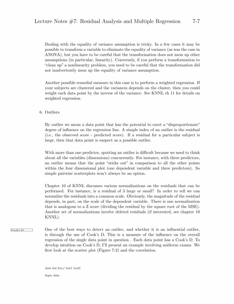
6. Outliers

By outlier we mean a data point that has the potential to exert a “disproportionate”degree of influence on the regression line. A simple index of an outlier is the residual(i.e., the observed score - predicted score). If a residual for a particular subject islarge, then that data point is suspect as a possible outlier.

With more than one predictor, spotting an outlier is difficult because we need to thinkabout all the variables (dimensions) concurrently. For instance, with three predictors,an outlier means that the point “sticks out” in comparison to all the other pointswithin the four dimensional plot (one dependent variable and three predictors). Sosimple pairwise scatterplots won’t always be an option.

Chapter 10 of KNNL discusses various normalizations on the residuals that can beperformed. For instance, is a residual of 3 large or small? In order to tell we cannormalize the residuals into a common scale. Obviously, the magnitude of the residualdepends, in part, on the scale of the dependent variable. There is one normalizationthat is analogous to a Z score (dividing the residual by the square root of the MSE).Another set of normalizations involve deleted residuals (if interested, see chapter 10KNNL).

One of the best ways to detect an outlier, and whether it is an influential outlier,Cook’s D

is through the use of Cook’s D. This is a measure of the influence on the overallregression of the single data point in question . Each data point has a Cook’s D. Todevelop intuition on Cook’s D, I’ll present an example involving midterm exams. Wefirst look at the scatter plot (Figure 7-2) and the correlation.

data list free/ test1 test2.

begin data


Figure 7-2: SPSS scatter plot

Plot of TEST2 with TEST1

TEST1

60504030

TE

ST

2

60

50

40

30

20

[data go here]end data.

plot format=regression/plot test2 with test1.

correlation test2 test1/print= twotail/statistics=all.

[OUTPUT FROM CORRELATION COMMAND]

Variable Cases Mean Std Dev

TEST2 28 39.0357 6.0399

TEST1 28 48.5714 4.2464

Variables Cases Cross-Prod Dev Variance-Covar

TEST2 TEST1 28 465.4286 17.2381

- - Correlation Coefficients - -


TEST2 TEST1

TEST2 1.0000 .6721

( 28) ( 28)

P= . P= .000

TEST1 .6721 1.0000

( 28) ( 28)

P= .000 P= .

(Coefficient / (Cases) / 2-tailed Significance)

Next, we’ll run a regression analysis. The syntax also shows you how to producescatter plots within the regression command (redundant with the plots we did above).Also, the last line of the command creates two new columns of data (labelled residand fits), which contain residuals and predicted Y values, respectively. You may needto use a “set width=132.” command before running the regression command to get allthe columns next to the “casewise” plot (and if using a windowing system, you mayneed to scroll horizontally as well to view the columns on your monitor).

Figure 7-3 displays the residuals plotted against the predictor variable. This plot wasgenerated by the plot command below.

regression variables= test1 test2/statistics = r anov coeff ci/dependent=test2/method=enter test1/residuals outliers(cook)/casewise=all sepred cook zpred sresid sdresid/scatterplot (test2, test1)/save resid(resid) pred(fits).

GRAPH/SCATTERPLOT(BIVAR)= test1 WITH resid.

comment: you can double click on the resulting residual plot to add ahorizontal reference line at Y=0 to provide a visual cue for thehorizontal band.

Multiple R .67211

R Square .45174

Adjusted R Square .43065

Standard Error 4.55742

Analysis of Variance

DF Sum of Squares Mean Square

Regression 1 444.94316 444.94316

Residual 26 540.02113 20.77004

F = 21.42235 Signif F = .0001

---------------------- Variables in the Equation -----------------------


Variable B SE B 95% Confdnce Intrvl B Beta

TEST1 .955986 .206547 .531423 1.380548 .672113

(Constant) -7.397887 10.069163 -28.095348 13.299573

----------- in ------------

Variable T Sig T

TEST1 4.628 .0001

(Constant) -.735 .4691

Casewise Plot of Standardized Residual

*: Selected M: Missing

Case TEST2 *PRED *RESID *ZPRED *SRESID *LEVER *COOK D *SEPRED

1 33.00 37.5335 -4.5335 -.3701 -1.0157 .0051 .0219 .9204

2 49.00 44.2254 4.7746 1.2784 1.1020 .0605 .0647 1.4139

3 40.00 38.4894 1.5106 -.1346 .3377 .0007 .0022 .8693

4 44.00 37.5335 6.4665 -.3701 1.4488 .0051 .0446 .9204

5 48.00 40.4014 7.5986 .3364 1.7016 .0042 .0602 .9104

6 36.00 35.6215 .3785 -.8411 .0858 .0262 .0002 1.1340

7 35.00 40.4014 -5.4014 .3364 -1.2096 .0042 .0304 .9104

8 50.00 46.1373 3.8627 1.7494 .9188 .1133 .0739 1.7595

9 46.00 44.2254 1.7746 1.2784 .4096 .0605 .0089 1.4139

10 37.00 38.4894 -1.4894 -.1346 -.3329 .0007 .0021 .8693

11 40.00 43.2694 -3.2694 1.0429 -.7463 .0403 .0229 1.2564

12 39.00 37.5335 1.4665 -.3701 .3286 .0051 .0023 .9204

13 32.00 28.9296 3.0704 -2.4895 .7860 .2295 .1115 2.3472

14 42.00 37.5335 4.4665 -.3701 1.0007 .0051 .0213 .9204

15 39.00 38.4894 .5106 -.1346 .1141 .0007 .0002 .8693

16 37.00 39.4454 -2.4454 .1009 -.5465 .0004 .0056 .8658

17 42.00 43.2694 -1.2694 1.0429 -.2898 .0403 .0035 1.2564

18 40.00 43.2694 -3.2694 1.0429 -.7463 .0403 .0229 1.2564

19 40.00 39.4454 .5546 .1009 .1239 .0004 .0003 .8658

20 47.00 42.3134 4.6866 .8074 1.0606 .0241 .0358 1.1150

21 37.00 30.8415 6.1585 -2.0185 1.4983 .1509 .2575 1.9688

22 34.00 38.4894 -4.4894 -.1346 -1.0035 .0007 .0190 .8693

23 21.00 33.7095 -12.7095 -1.3120 -2.9387 .0638 .4770 1.4374

24 40.00 40.4014 -.4014 .3364 -.0899 .0042 .0002 .9104

25 34.00 39.4454 -5.4454 .1009 -1.2170 .0004 .0277 .8658

26 39.00 42.3134 -3.3134 .8074 -.7498 .0241 .0179 1.1150

27 38.00 38.4894 -.4894 -.1346 -.1094 .0007 .0002 .8693

28 34.00 32.7535 1.2465 -1.5475 .2923 .0887 .0061 1.6075

Residuals Statistics:

Min Max Mean Std Dev N

*PRED 28.9296 46.1373 39.0357 4.0595 28

*ZPRED -2.4895 1.7494 .0000 1.0000 28

*SEPRED .8658 2.3472 1.1585 .3830 28

*ADJPRED 27.8211 45.4607 38.9605 4.1869 28

*RESID -12.7095 7.5986 .0000 4.4722 28

*ZRESID -2.7888 1.6673 .0000 .9813 28

*SRESID -2.9387 1.7016 .0076 1.0249 28


Figure 7-3: SPSS scatter plot

Plot of RESID with TEST1

TEST1

60504030

Res

idua

l

8

6

4

2

0

-2

-4

-6

*DRESID -14.1134 7.9144 .0752 4.8862 28

*SDRESID -3.5262 1.7700 -.0088 1.0989 28

*MAHAL .0102 6.1977 .9643 1.4580 28

*COOK D .0002 .4770 .0479 .0987 28

*LEVER .0004 .2295 .0357 .0540 28

Total Cases = 28

It appears that subject 23 is an outlier because the residual (-12.71) is much largerin magnitude than any other residual. We’ll omit that subject for now and redo theanalysis. That particular subject was the only one to have a test2 score of 21 so wecan conveniently select that subject out by asking SPSS to not use subjects whosetest2 score equals 21. Had the data file included a subject ID index (e.g., a subjectnumber), then it would have been more efficient to select directly on subject number.


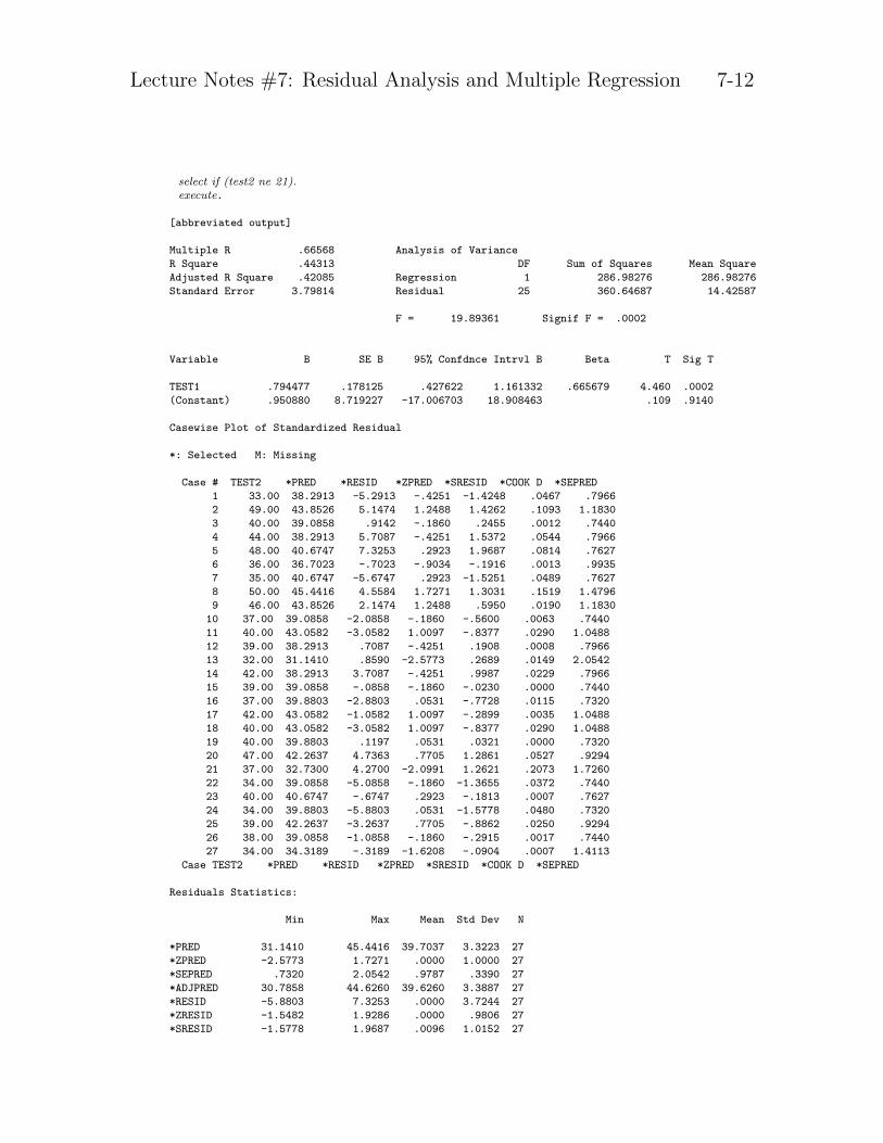
select if (test2 ne 21).execute.

[abbreviated output]

Multiple R .66568 Analysis of Variance

R Square .44313 DF Sum of Squares Mean Square

Adjusted R Square .42085 Regression 1 286.98276 286.98276

Standard Error 3.79814 Residual 25 360.64687 14.42587

F = 19.89361 Signif F = .0002

Variable B SE B 95% Confdnce Intrvl B Beta T Sig T

TEST1 .794477 .178125 .427622 1.161332 .665679 4.460 .0002

(Constant) .950880 8.719227 -17.006703 18.908463 .109 .9140

Casewise Plot of Standardized Residual

*: Selected M: Missing

Case # TEST2 *PRED *RESID *ZPRED *SRESID *COOK D *SEPRED

1 33.00 38.2913 -5.2913 -.4251 -1.4248 .0467 .7966

2 49.00 43.8526 5.1474 1.2488 1.4262 .1093 1.1830

3 40.00 39.0858 .9142 -.1860 .2455 .0012 .7440

4 44.00 38.2913 5.7087 -.4251 1.5372 .0544 .7966

5 48.00 40.6747 7.3253 .2923 1.9687 .0814 .7627

6 36.00 36.7023 -.7023 -.9034 -.1916 .0013 .9935

7 35.00 40.6747 -5.6747 .2923 -1.5251 .0489 .7627

8 50.00 45.4416 4.5584 1.7271 1.3031 .1519 1.4796

9 46.00 43.8526 2.1474 1.2488 .5950 .0190 1.1830

10 37.00 39.0858 -2.0858 -.1860 -.5600 .0063 .7440

11 40.00 43.0582 -3.0582 1.0097 -.8377 .0290 1.0488

12 39.00 38.2913 .7087 -.4251 .1908 .0008 .7966

13 32.00 31.1410 .8590 -2.5773 .2689 .0149 2.0542

14 42.00 38.2913 3.7087 -.4251 .9987 .0229 .7966

15 39.00 39.0858 -.0858 -.1860 -.0230 .0000 .7440

16 37.00 39.8803 -2.8803 .0531 -.7728 .0115 .7320

17 42.00 43.0582 -1.0582 1.0097 -.2899 .0035 1.0488

18 40.00 43.0582 -3.0582 1.0097 -.8377 .0290 1.0488

19 40.00 39.8803 .1197 .0531 .0321 .0000 .7320

20 47.00 42.2637 4.7363 .7705 1.2861 .0527 .9294

21 37.00 32.7300 4.2700 -2.0991 1.2621 .2073 1.7260

22 34.00 39.0858 -5.0858 -.1860 -1.3655 .0372 .7440

23 40.00 40.6747 -.6747 .2923 -.1813 .0007 .7627

24 34.00 39.8803 -5.8803 .0531 -1.5778 .0480 .7320

25 39.00 42.2637 -3.2637 .7705 -.8862 .0250 .9294

26 38.00 39.0858 -1.0858 -.1860 -.2915 .0017 .7440

27 34.00 34.3189 -.3189 -1.6208 -.0904 .0007 1.4113

Case TEST2 *PRED *RESID *ZPRED *SRESID *COOK D *SEPRED

Residuals Statistics:

Min Max Mean Std Dev N

*PRED 31.1410 45.4416 39.7037 3.3223 27

*ZPRED -2.5773 1.7271 .0000 1.0000 27

*SEPRED .7320 2.0542 .9787 .3390 27

*ADJPRED 30.7858 44.6260 39.6260 3.3887 27

*RESID -5.8803 7.3253 .0000 3.7244 27

*ZRESID -1.5482 1.9286 .0000 .9806 27

*SRESID -1.5778 1.9687 .0096 1.0152 27


*DRESID -6.1071 7.6331 .0777 3.9971 27

*SDRESID -1.6291 2.0985 .0146 1.0393 27

*MAHAL .0028 6.6426 .9630 1.5666 27

*COOK D .0000 .2073 .0372 .0499 27

*LEVER .0001 .2555 .0370 .0603 27

Total Cases = 27

In the two regressions the slopes are comparable but the intercepts differ a great dealin absolute terms. Further, the R2s are not very across the two regressions suggestingthat the two regressions are comparable. Perhaps that point we suspected to be anoutlier is not very influential because its presence or absence does little to change theresulting regression.

The main things to note in this example are the effects of the outlier on the parameterestimates and how the residuals, and associated printouts, were used to decipher wherethe assumptions were being violated. The way we detected whether this suspectedpoint was an outlier was to remove it and re-run the regression. We compared theeffects of the model with the suspected outlier included and the model without thesuspected outlier. For this example, both cases yielded comparable results. So, forthis example including the outlier will not do too much damage.

I am not advocating that outliers be dropped in data analysis. Rather, Isimply compared two different regressions (one with the outlier and one without) tosee whether the results differed. The comparison of these two regressions lets meassess how much “influence” the particular data point has on the overall regression.This time the two regressions were similar so I feel pretty confident in reporting resultswith all subjects. In this example the outlier appears to have little impact on the finalresult.

This idea of comparing the model with the outlier and the model without the outliercan be extended. Why not do this for every data point? First, perform one regressionwith all the data included. Then perform N different regressions; for each regressiona single data point is removed. This would tell us how “influential” each data point ison the regression line. Luckily, there is a quick way of doing this computation (if youhad 200 subjects, the technique I just outlined would require 201 separate regressions).The quick way is Cook’s D (D stands for distance). The formula for Cook’s D involvesquite a bit of matrix algebra so I won’t present it here (see KNNL for a derivation).Cook’s D is basically a measure of the difference between the regression one gets byincluding subject i and the regression one gets by omitting subject i. So, each subjectgets his or her own Cook’s D. A subject’s individual D is an index of how influentialthat subject’s data are on the regression line. Large values of Cook’s D indicate thatthe particular data point (subject) has a big effect on the regression equation. Cook’s


D is influenced both by the residual and the leverage1 of the predictors.

Determining what constitutes a large value of Cook’s D involves calculating the sam-pling distribution for F, so we’ll just have to make good guesses as to constitutes highvalues of Cook’s D. A rule of thumb is to look for Cook’s D values that are relativelygreater than the majority of the D’s in the sample. Some people propose a simple ruleof thumb, such as any Cook’s D greater than 4/N is a potential influential outlier. inthis example with 27 observations 4/27=.148 so two points are potential influentialoutliers.

Another strategy for determining key values of Cooks D is to use the F table to setup critical values. Use α = 0.50 (not 0.05), the numerator degrees of freedom arethe number of parameters in the structural model (including the intercept), and thedenominator degrees of freedom are N minus the number of parameters (the same dfassociated with MSE). For example, with two predictors (so a total of 3 parametersincluding the intercept), 24 df in the error, and α = .50, we find a tabled value of0.812.

In the present example, there was one predictor so there were 2 parameters includingthe intercept, there were 26 residual degrees of freedom. The F value correspondingto .50 with 2,26 degrees of freedom is .712. This gives a numerical benchmark forCook’s D in this particular example: any observed Cook’s D greater than 0.712 issuspect because it might be an influential outlier.

One could use the built in F function in SPSS (or Excel) to find the necessary valueof F . In SPSS, for example, with the menu system under TRANSFORM-COMPUTEyou will find a list of functions. Select IDF.F. For this example you would typeIDF.F(.50,2,26), define the new variable you want the output to go into, and click onOK. Or, in the syntax window type this command and you will get a new columnof identical numbers that give the F cutoff (“Fcrit” is an arbitrary name for the newcolumn this command creates).

compute Fcrit = idf.f(.50, 2, 26).

execute.

An alternative but identical approach to finding the critical Cook’s D value would beto use the inverse F function on the column of Cook D scores to find the cumulative

1For a definition of leverage see KNNL. It turns out that SPSS has it’s own definition of leverage. SPSSuses a centered leverage, i.e., hi - 1

n where n is the number of subjects. Most people just use hi. SPSS printsout the leverage values as part of the casewise plot (labeled LEVER; in most versions of SPSS you have towrite “lever” on the casewise line to get this to print out).


area under the F . That is, if you save Cook’s D scores in a new column called cook(or any other arbitrary variable name you like), then you can run this command onthat column of saved Cook D scores:

compute pval = cdf.f(cook, 2, 26).

execute.

This syntax will produce a new column of “pvals”. Look for any “pval” greater than.50 and those are potential influential outliers. Both the cdf.f and idf.f approaches willlead to identical conclusions based on the F test.

This logic of comparing regressions with and without a data point can also be extendedto examine the effect on individual regression parameters like intercept and slopes.Cook’s D focuses on the effect of the entire regression rather than individual βs. Thereis an analogous measure DFBETA that examines the effect of each single data pointon each regression parameter. SPSS computes the change for each β in standardizedunits of removing each data point. To get this within SPSS just add a

\SAVE SDBETA(name)

to your regression syntax. If you have two predictors, this command will create threenew columns in your data file labeled name1, name2 and name3 for the standardizeddifference in beta of that point on each of the intercept and the two predictors. A valueof say -.1 means that particular beta drops .1 standard error units when that datapoint is added as compared to when it is omitted. Some people treat a standardizedDFBETA greater than one a potential influential outlier, others us the rule 2/sqrt(N),so any standardized DFBETA greater than 2/sqrt(N) becomes a suspicious influentialoutlier.

7. What to do if you have influential outliers?

As I said before, don’t automatically drop the outliers. Check whether there was adata entry error or if something was different about that particular data collectionsession (e.g., a new RA’s first subject).

If there is a small cluster of outliers, you may want to check whether there is somethinginformative about this small group. It could be error, but it could be a signal abouta relatively small class of participants. For example, in a dataset with 250 familiesthere may be 6 kids who act out aggressively, and these may be the kids who are athigh risk.


You can run nonparametric or robust regression, which is not as sensitive to outliersas the typical regressions we run though can exhibit lower power.

8. Relation between the two sample t test and regression with one predictor.

Now I’ll show the connection between ANOVA and regression.

Let’s start off with a simple example with two experimental groups. Here are the data.Note the three extra columns. These columns represent three different ways to codethe predictor variable. All are fine as long as you keep track of the values you used(much like interpreting a contrast value that depends on the particular coefficients).The means for the two groups are 8.56 and 5.06, the grand mean is 6.81, and thetreatment effect α is 1.75. Think about what each of the three scatterplots (the firstcolumn on the y-axis and each of the three remaining columns on separate x-axes)will look like.

5.4 1 1 1

6.2 1 1 1

3.1 1 1 1

3.8 1 1 1

6.5 1 1 1

5.8 1 1 1

6.4 1 1 1

4.5 1 1 1

4.9 1 1 1

4.0 1 1 1

8.8 0 -1 2

9.5 0 -1 2

10.6 0 -1 2

9.6 0 -1 2

7.5 0 -1 2

6.9 0 -1 2

7.4 0 -1 2

6.5 0 -1 2

10.5 0 -1 2

8.3 0 -1 2

data list free / dv dummy contrast group.

REGRESSION USING 0 AND 1 TO CODE FOR GROUPS

regression variables = dv dummy

/statistics = r anova coeff ci

/dependent = dv

/method=enter dummy.





F = 34.23063 Signif F = .0000



DUMMY -3.500000 .598220 -4.756813 -2.243187 -.809552 -5.851 .0000

(Constant) 8.560000 .423005 7.671299 9.448701 20.236 .0000

A SECOND REGRESSION USING 1 AND -1 TO CODE FOR GROUPS

regression variables = dv contrast


/dependent = dv

/method=enter contrast.





F = 34.23063 Signif F = .0000


CONTRAST -1.750000 .299110 -2.378406 -1.121594 -.809552 -5.851 .0000

(Constant) 6.810000 .299110 6.181594 7.438406 22.768 .0000

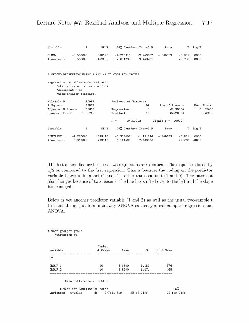
The test of significance for these two regressions are identical. The slope is reduced by1/2 as compared to the first regression. This is because the coding on the predictorvariable is two units apart (1 and -1) rather than one unit (1 and 0). The interceptalso changes because of two reasons: the line has shifted over to the left and the slopehas changed.

Below is yet another predictor variable (1 and 2) as well as the usual two-sample ttest and the output from a oneway ANOVA so that you can compare regression andANOVA.

t-test groups= group

/variables dv.

Number

Variable of Cases Mean SD SE of Mean

-----------------------------------------------------------------------

DV

GROUP 1 10 5.0600 1.189 .376

GROUP 2 10 8.5600 1.471 .465

-----------------------------------------------------------------------

Mean Difference = -3.5000

t-test for Equality of Means 95%

Variances t-value df 2-Tail Sig SE of Diff CI for Diff


-------------------------------------------------------------------------------

Equal -5.85 18 .000 .598 (-4.757, -2.243)

Unequal -5.85 17.24 .000 .598 (-4.761, -2.239)

oneway dv by group(1,2)

ANALYSIS OF VARIANCE

SUM OF MEAN F F

SOURCE D.F. SQUARES SQUARES RATIO PROB.

BETWEEN GROUPS 1 61.2500 61.2500 34.2306 .0000

WITHIN GROUPS 18 32.2080 1.7893

TOTAL 19 93.4580

A THIRD REGRESSION USING A CODE OF 1 AND 2 FOR THE TWO GROUPS

regression variables = dv group


/dependent = dv

/method=enter group.





F = 34.23063 Signif F = .0000


GROUP 3.500000 .598220 2.243187 4.756813 .809552 5.851 .0000

(Constant) 1.560000 .945868 -.427195 3.547195 1.649 .1164

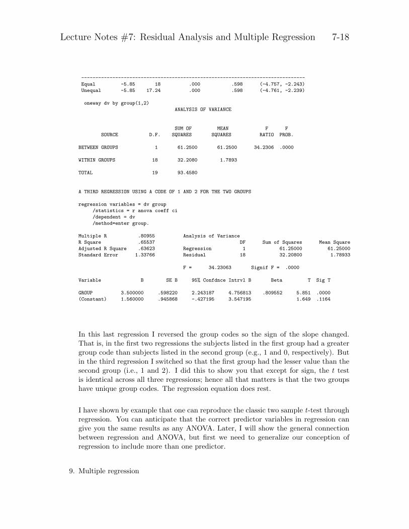
In this last regression I reversed the group codes so the sign of the slope changed.That is, in the first two regressions the subjects listed in the first group had a greatergroup code than subjects listed in the second group (e.g., 1 and 0, respectively). Butin the third regression I switched so that the first group had the lesser value than thesecond group (i.e., 1 and 2). I did this to show you that except for sign, the t testis identical across all three regressions; hence all that matters is that the two groupshave unique group codes. The regression equation does rest.

I have shown by example that one can reproduce the classic two sample t-test throughregression. You can anticipate that the correct predictor variables in regression cangive you the same results as any ANOVA. Later, I will show the general connectionbetween regression and ANOVA, but first we need to generalize our conception ofregression to include more than one predictor.

9. Multiple regression


Multiple regression is a simple and natural extension of what we have been talkingabout with one predictor variable. Multiple regression permits any number of (addi-tive) predictor variables. Multiple regression simply means “multiple predictors.”

The model is similar to the case with one predictor; it just has more X’s and β’s.

Y = β0 + β1X1 + β2X2 + β3X3 . . .+ βpXp + ε (7-3)

where p is the number of predictor variables. The assumptions are the same as forlinear regression with one predictor. Each βi corresponds to the slope on the ithvariable holding all other predictor variables constant (i.e., the “unique” slope, or thepartial slope). This idea corresponds to the partial derivative in calculus. Ideally,the predictors should not be correlated with the other predictors because this createsmulticollinearity problems–the standard error of the slope will be larger than it shouldbe. More on this “multicollinearity problem” later.

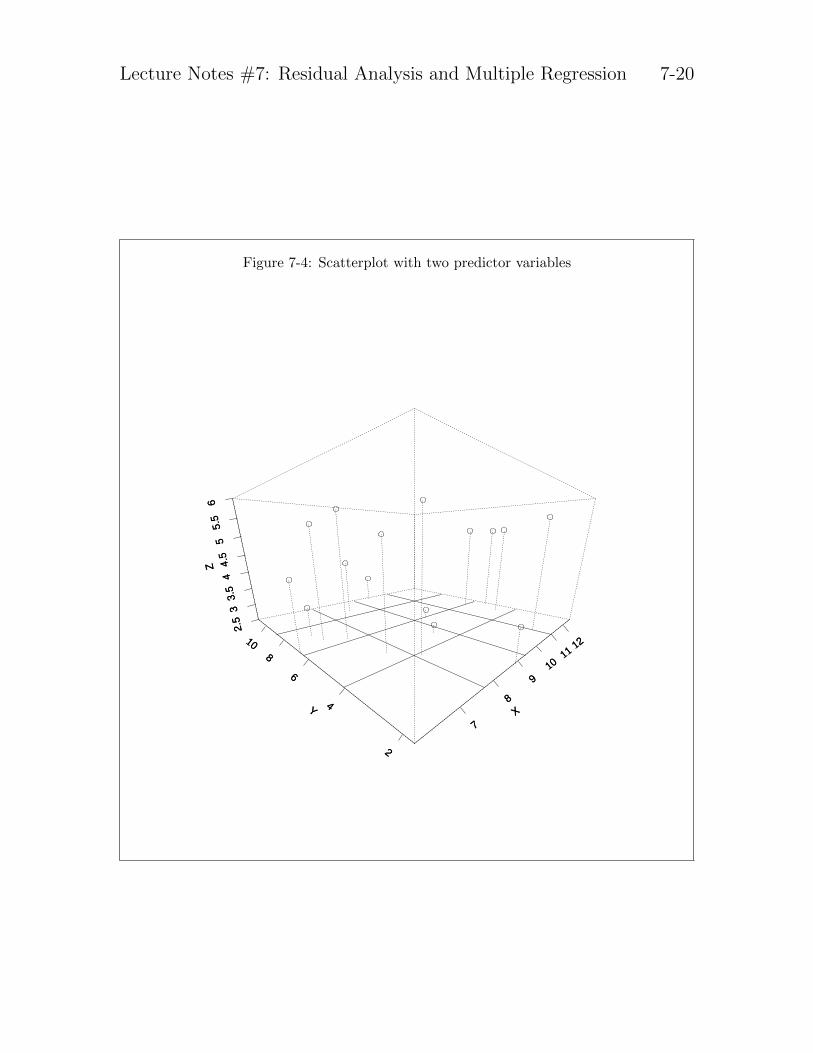
With two predictors there is a three dimensional scatterplot that corresponds to theregression problem. Figure 7-4 shows a scatterplot in three dimensions. The threedimensions refer to the predictors and the two dependent variable, with the points inthe plot representing subjects.

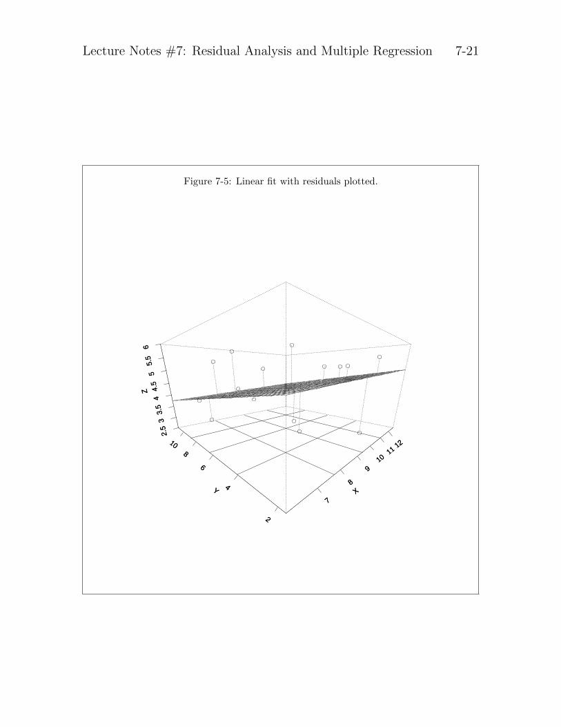
For two predictors, the regression is finding the plane that minimizes the residuals.Figure 7-5 shows the same scatter plot but with a plane of best fit. The analog withthe pegboard demonstration should be obvious–rather than fitting a line there is nowa plane.

Three or more predictor variables are difficult to display in a plot because we need morethan three dimensions but the idea and intuition scales to any number of dimensions.

Variance decomposition is also extended to the case of multiple regression. The degreesof freedom in the numerator take into account the number of predictors. The F ratiofrom the source table is interpreted as whether all the variables as a set account fora significant proportion of the variability in the dependent variable. That is, theF ratio is comparing “the model” as a whole (MSregression) to “what’s left over”

(MSresiduals). This corresponds to the simple ANOVA design that decomposed sumsof squares into between and within components. The form of the multiple regressionsource table is

SS df MS F

SSR=∑

(Yi − Y)2 number of parameters - 1 SSR/df MSR/MSE

SSE=∑

(Yi − Yi)2 N - number of parameters SSE/df


Figure 7-4: Scatterplot with two predictor variables

7

8

910

1112

X

2

4

6

8

10

Y

2.5

33.

54

4.5

55.

56

Z


Figure 7-5: Linear fit with residuals plotted.

7

8

910

1112

X

2

4

6

8

10

Y

2.5

33.

54

4.5

55.

56

Z


The value R2 is simplySSregression

SStotal. This value is interpreted as the percentage of

the variance in Y that can be accounted for by the set of X variables. Recall thepie chart we played with earlier in the term with ANOVA. The square root of R2,sometimes denoted ryy, is the correlation between the observed data and the fittedvalues. Both are indices of how well a linear model fits the data.

The F given by MSR/MSE is an omnibus test that shows how well the model asa whole (all predictors as an aggregate) fit the data. This F tests whether R2 issignificantly different from zero. As with all omnibus tests, this particular F is notvery useful. We usually care more about how specific predictors are performing,especially in relation to other predictors. Thus, we are usually interested in eachslope. This is analogous to the “I hats” from contrasts in ANOVA.

Each slope is an index of the predictor’s unique contribution. In a two predictorregression there will, of course, be two slopes. The interpretation of these two slopesis as follows. The slope β1 is attached to predictor X1 and the slope β2 is attachedto predictor X2. The slope β1 can be interpreted as follows: if predictor X2 is heldconstant and predictor X1 increases by one unit, then a change of β1 will result in thecriterion variable Y. Similarly, the slope β2 means that if predictor X1 is held constantand predictor X2 increases by one unit, then a change of β2 will result in the criterionvariable Y. Thus, each slope is an index of the unique contribution of each predictorvariable to the criterion variable Y. This logic extends to any number of predictorssuch that the slope βi refers to the unique contribution of variable i holding all othervariables constant.

We can test each individual slope βi against the null hypothesis that the populationβi = 0 as well as build confidence intervals around the estimates of the slopes. Thetest for each slope is a test of whether the predictor variable accounts for a significantunique portion of the variance in the criterion variable Y. SPSS output convenientlyprovides both the estimates of the β parameters as well as their standard errors. Thet test is the ratio of the slope estimate over its standard error and the confidenceinterval is the usual estimate plus or minus the margin of error.

We need to be careful when interpreting the t test for each βi because those testsdepend on the intercorrelations among the predictor variables. If the predictors arecorrelated, then there is no single way to assess the unique contribution of each pre-dictor separately. That is, when a correlation between predictors is present, there isno sensible way to “hold all other predictors constant”. Thus, the presence of correla-tions between the predictor variables introduces redundancy. This problem is similarto what we encountered with unequal sample sizes in the factorial ANOVA.

As we saw with simple linear regression, the multiple regression function (Equation 7-


3) can be used to make predictions, both mean E(Y) and individual Y. There is alsoa standard error prediction (SEPRED) corresponding to each subject.

Those interested in a full explanation of the relevant formulae should consult KNNLwho develop the matrix algebra approach to multiple regression. The value of matrixnotation becomes clear when dealing with multiple regression. I will not emphasizethe details of definitional and computational formulae for multiple regression in thisclass because they are generalizations of the simple linear regression case using ma-trix algebra concepts. If you understand the case for simple linear regression, thenyou understand multiple regression too. In this class I will emphasize the ability tointerpret the results from a regression rather than how to compute a regression.

10. Testing “sets of variables”

Sometimes one wants to test whether a subset of predictor variables increases pre-dictability. For example, I may have a regression with five variables. I want to testwhether the last three variables increase the fit to the data (i.e., minimize the resid-uals, or equivalently, increase R2) significantly over and above whatever the first twovariables are already doing. An example of this is with the use of blocking variables.Suppose I have two variables that I want to use as blocking factors to soak up er-ror variance and three other variables of interest. I am mainly interested in whetherthese latter three variables can predict the dependent variable over and above the twoblocking factors.

The way to do this is through the “increment in R2 test.” You do two separateregression equations. One is the full model with five variables included; the other isthe reduced model with the particular subset under consideration omitted from theregression. You then test the difference in R2; that is, how much did R2 increase fromthe reduced to the full regression. The formula is

F =

SSE(R) - SSE(F)dfreduced - dffull

SSE(F)dffull

(7-4)

=

(SSE(R) - SSE(F)

SSE(F)

)(dffull

dfreduced - dffull

)(7-5)

where SSE(R) and SSE(F) are the sum of squares for the reduced and full models,respectively, and dfred and dffull are the degrees of freedom (for the denominator)in the reduced regression and the full regression, respectively. In Lecture Notes #8,I’ll present a version of this same equation in terms of R2. In the example with theblocking variables, the full regression would include all five predictors and the reducedregression would include only the two predictors that are being used as blocking factors(i.e., the reduced regression omits the three variables of interest). This F test is


comparing the difference in error between the two models. This is the approach theMaxwell and Delaney used throughout their book for explaining ANOVA.

The observed F in Equation 7-4 is compared to the tabled F, where dfred-dfful thedegrees of freedom for the numerator and dfful is the degrees of freedom for thedenominator.

The F test in Equation 7-4 provides an omnibus test for whether the omitted variables(the ones that appear in the full model but not the reduced model) account for asignificant portion of the variance in the criterion variable Y. Thus, in my examplewith the two blocking factors and three variables of interest, the F test in Equation 7-4 tells me whether the three predictor variables of interest as a set account for asignificant portion of the variance in Y, over and above that previously accountedfor by the two blocking factors. As such, this F test is an omnibus test because itgives information about the set of three variables rather than information about theseparate usefulness of each predictor.

If you think about it, wouldn’t it be possible to do an increment in R2 for each in-dependent variable separately (i.e., looking at each predictor variable’s “independent”contribution to R2)? In other words, the full regression includes all p predictors andone performs a sequence of reduced regressions each with p - 1 predictors, where foreach of the reduced regressions one of the predictor variables is omitted. It turns outthat this is a sensible idea because it gives the significance test for the unique contri-bution of each predictor variable. Earlier I noted that the t-test associated with theslope provides a test for the unique contribution of the variable associated with thatslope. As you would expect, the two tests (t-test on the individual slope or the F-testusing Equation 7-4 where only one variable is omitted in the reduced regression) areidentical; both are testing the unique contribute of that particular predictor variable.


Appendix 1: Relevant R syntax

Cook’s distance

If you save the lm() output, then you can run the cooks.distance() command on the output

lm.out <- lm(y~x)

c.d <- cooks.distance(lm.out)

Now you can treat c.d like a variable that you can plot or perform other computations.

To find the critical F for Cook’s at .50 you can use this command (following the examplegiven earlier in the lecture notes)

qf(.5,3,24)

R has an entire suite of additional diagnostics such as the dfbetas(), rstandard(), rstu-dent(), etc. The R command dfbetas() is the standardized version, whereas, dfbeta() is theunstandardized version.

Multiple Regression

It is easy to perform multiple regression in R. Just list all predictors in the lm command. Ifyou want a full factorial design you can use the asterisk instead of plus; if you want specificinteractions you can use the colon (see Lecture Notes 4 for a similar description in the caseof the aov() command).

lm.out <- lm(y~ x1 + x2 + x3 + x4)

summary(lm.out)

cooks.distance(lm.out)

Lecture Notes #7: Residual Analysis and Multiple ...gonzo/coursenotes/file7.pdfmore examples of this...

Documents

Transcript of Lecture Notes #7: Residual Analysis and Multiple ...gonzo/coursenotes/file7.pdfmore examples of this...