Lecture Five: Star Formation in M -3 Galaxies…etolstoy/gfe11/lec5.pdf · Star Formation in...
12
Lecture Five: Mo, vd Bosch & White, chapters 9, 10 literature Tuesday 1 st March Star Formation in Galaxies… Physical Process Star formation defines the visible properties of galaxies and this means that any theory of galaxy formation needs to include a theory of how stars form… A full understanding of star formation in a cosmological framework is challenging – the typical mass of gas in a galaxy is ~10 11 M ! with a density of ~10 -24 gcm -3 , and for a typical star this is ~1M ! and ~1gcm -3 . What does Galactic star formation tell us? • Star formation occurs in molecular clouds • More precisely, it occurs within the dense parts of molecular clouds This raises the question of whether star formation occurs because the gas is dense or because it is molecular or both Why molecular gas? only molecular gas can cool below 100 K and therefore collapse under its own gravity: Jeans criteria, Bonnor-Ebert atomic gas does not emit efficiently at these temperatures but molecular gas does, mostly with roto-vibrational transitions. the more its emits the more it cools, the more its density increases (so gravity increases). at some point gravity will exceeds the pressure, the equilibrium is broken and the collapse starts.
Transcript of Lecture Five: Star Formation in M -3 Galaxies…etolstoy/gfe11/lec5.pdf · Star Formation in...

Lecture Five:
Mo, vd Bosch & White, chapters 9, 10
literature Tuesday 1st March
Star Formation in Galaxies…!
Physical Process Star formation defines the visible properties of galaxies and
this means that any theory of galaxy formation needs to include a theory of how stars form…
A full understanding of star formation in a cosmological
framework is challenging – the typical mass of gas in a
galaxy is ~1011M!
with a density of ~10-24 gcm-3, and for a typical star this is ~1M
! and ~1gcm-3.
What does Galactic star formation tell us?!
•! Star formation occurs in molecular
clouds
•! More precisely, it occurs within the
dense parts of molecular clouds
This raises the question of whether star formation occurs
because the gas is dense or because it is molecular or
both
Why molecular gas?!
only molecular gas can cool below 100 K and
therefore collapse under its own gravity:
Jeans criteria, Bonnor-Ebert
atomic gas does not emit efficiently at these
temperatures but molecular gas does, mostly with
roto-vibrational transitions. the more its emits the
more it cools, the more its density increases (so gravity increases). at some point gravity will
exceeds the pressure, the equilibrium is broken
and the collapse starts.

Star Formation in molecular clouds!
Molecular gas in the plane of the
Milky Way
Molecular core
Simplified view of IMF!•! Field Star IMF is within errors same as that
inferred for Orion Nebula Cluster and other nearby star forming regions
•! It has a power law (Salpeter) down to about 0.5-1 M
! with most mass in solar mass stars
but most luminosity at high M
•! Evidence for deviations from standard IMF in some Gal. Center clusters
Bastian et al. 2010 ARAA
One possible explanation of the IMF!
•! It reflects the mass distribution of the
cloud fragments or cores in the
molecular cloud
•! The “typical” mass of around 1 M! then
reflects the Jeans Mass (very T
dependent)
M(JEANS) ~ T3/2 n-1/2

The origin of the Initial Mass
Function
(see also Testi & Sargent 1998; Motte et al. 2001) !
Submm continuum surveys of nearby protoclusters suggest that the mass !
distribution of pre-stellar condensations mimics the form of the stellar IMF
NGC2068 protocluster at 850 µm!
Motte et al. 2001!
Condensations mass spectrum in ! Oph!
"! The IMF is at least partly determined by fragmentation at the pre-stellar
stage.!
Consequences for extragalactic SF!
•! If fragmentation is fundamental in determining the
IMF, the Jeans Mass and hence the temperature
may determine the critical turn-over mass
•! This could cause the IMF in galactic nuclei to be
more biased towards high mass ???
•! Temperatures in Galactic Center clouds are high
Galactic timescale for Star
Formation tSF
•! One might naturally think it was the free-fall time at the mean density of molecular clouds
•! But as pointed out in the 70s by Zuckerman and Evans, real galactic SF Rate is lower (tSF=109 yr) than from free fall time (tff roughly 106 years)
•! This has given rise to two classes of theories: –! “slow”: including “ambipolar diffusion” modulated theories.
–! “inefficient”: turbulence, HII regions and winds
Conclusions
•! Extragalactic star formation may well be just
galactic writ large
•! But we do not understand what determines
the efficiencies and timescales
•! Of course the IMF might be playing tricks

Stars form in spiral arms!M33 Spitzer Image Physical Process We assume that for understanding large scale effects on
galaxy evolution we don’t need to go into the specific small scale details of star formation.
GLOBAL PROPERTIES
Need to understand how the GLOBAL properties of star
formation averaged over a large volume of gas, depend on the GLOBAL properties of the gas, such as mass, density,
temperature and chemical composition.
Empirical Star Formation “Laws”
SFR, !, in terms of mass in stars formed per unit area per unit time
Gas consumption time,
Since the most obvious requirement for star formation is the presence of gas, it is only
logical to look at the relation between SFR and surface density of gas:
Schmidt (1959)
Kennicutt-Schmidt law!
Kennicutt (1998) ApJ, 498, 541
The study of star formation in normal
spiral galaxies and also starbursts
have shown Schmidt is a surprisingly
good description of global SFRs
(averaged over entire SF disc) –

Interpretation!
Kennicutt (1998) ApJ, 498, 541
SFR is controlled by the self-gravity of the gas? This would mean that the rate of
star formation will be proportional to the gas mass divided by the time scale for
gravitational collapse (free-fall time).
" is the free-fall time of the gas divided by gas
consumption time, or star formation efficiency
If all galaxies have approx. same scale height, this implies:
in good agreement with empirical law
However, this interpretation implies
Which suggests that self gravity isn’t the only important process.
Perhaps only a small fraction of gas participates in star formation, or the star formation
time scale is #/". In either case – additional physics required to explain empirical law.
Dynamical time scale!
Kennicutt (1998) ApJ, 498, 541
In addition to the Schmidt law – there
is an equally strong correlation
between star formation rate and the
gas surface density divided by the
dynamical time
defined as the orbital time at the outer
radius R of the relevant star forming
region.
$ is the circular frequency
This implies 10% of available gas forms stars per orbital time
The HI Nearby Galaxy Survey: (THINGS) HI maps
CO maps of Nearby Galaxies H2 maps
GALEX far-UV maps current SFR
SPITZER IR nearby galaxy survey (SINGS) past SFR
Walter et al. (2008)
Gil Paz et al. (2007)
Kennicutt et al. (2003)
Helfer et al. (2003); Leroy et al. (2008)
Nearby Galaxy Surveys!
This combination yields sensitive, spatially resolved measurements of kinematics, gas
surface density, stellar surface density, and SFR surface density across the entire
optical disks of 23 spiral and irregular galaxies.
The observation that HI in disk galaxies typically extends well beyond the optical disk
suggests that star formation is somehow suppressed in the outer disk: truncated

Small Scale Star Formation Measurements!
Bigiel et al. (2008) AJ, 136, 2846
Molecular Schmidt law HI saturates at ~9 M!
pc-2
gas in excess is only
molecular
No universal relation between
total gas density and sfr
!SFR is found to drop whenever the surface densities of cold gas drop below 10M!
pc-2.
Leroy et al. (2008) AJ, 136, 2782
Formation of cold phase: where T drops
to ~500K, the molecular fraction reaches
10-3 and Qgas ~ 1. Good indicators that cold HI is common and H2 formation is
efficient.
Schaye (2004)
Shear, limit the formation of
molecular clouds
Hunter et al. (1998)
Instability of gas disk in presence of
stars:
Rafikov (2001)
Gravitational instability:
Martin & Kennicutt (2001)
Star Formation Thesholds!
Local Star Formation Laws!
Leroy et al. (2008) AJ, 136, 2782
Global star formation laws averaged over whole disk – really need to understand the
importance of different physical parameters (gas density, orbital time scales) on smaller
spatial scales.
This relation valid from galaxy to galaxy but not within a galaxy, meaning that the orbital
time seems to have no impact on LOCAL star-formation efficiency.
on the other hand does change within a galaxy.
It can be seen that looking at the relations with atomic and molecular gas separately,
and molecular gas correlated much better with SFR.
A single power law is a poor fit, as there is a break at low gas surface densities. This
corresponds to an abrupt truncation in the SFR.
Schmidt law for molecular gas
Two laws: 1. for transformation from atomic into molecular gas 2. formation of stars from
molecular gas
Bigiel et al. (2008) AJ, 136, 2846
Estimating stellar masses By fitting a set of model predictions to
observational data (magnitudes,
spectral features), finding the scaling
factor required to reproduce the
observed fluxes we can estimate the
stellar mass of a galaxy (and it is usually
well constrained - e.g. Bell & de Jong 2001).
This has led to stellar mass
having become the most
important independent
variable in galaxy evolution
studies.

Star Formation Tracers!
Predicted spectra of coeval stellar population: 1, 10, 100, 400 Myr, 1, 4, 13 Gyr
Solar metallicity & Salpeter IMF
Lyman break D4000 break (depends strongly on Z)
Star formation tracers!
Steller Masses & SFHs!We see how we can determine the SED of a galaxy from a SFH. The inverse – can
we determine physical properties of galaxies (e.g., stellar masses and SFHs) from quantities that are directly observed (e.g., luminosity, spectrum). These observed
quantities are convolutions of the SFH, IMF, dust extinction, etc.
Exponential SFHs of the form:
characteristic SF time scale
Bell & de Jong (2001) ApJ, 550, 212
Sloan/2MASS colours to M/L!
Bell et al (2003) ApJS, 149, 289

Star formation diagnostics! Kennicutt (1998) ARAA, 36, 189
UV Continuum (1250-2500A) :
Number of massive stars in a galaxy is directly proportional to the current SFR, as long
as it is not absorbed on the way. Only possible from the ground for z=1-5. For z<1 need
space telescope. Assuming time scale ~108 yr, or longer:
Nebular Emission Lines:
The ISM around young, massive stars is ionised by Lyman continuum photons produced
by these stars, giving rise to HII regions. The recombination of this ionised gas produces
H emission lines (e.g., H% but also H&, P%, P&, Br%, Br'), which can be used as SFR
diagnostic, because their flux is proportional to the Lyman continuum flux from young
(<2x10⁷yr) massive (>10M!
) stars.
Forbidden lines:
For galaxies with z>0.5, H% emission is redshifted out of optical. The strongest feature in
the blue is [OII](3727 forbidden line doublet. Unfortunately luminosities do not depends
only on the local radiation field, but also the ionization state and metallicity of ISM. It has
been successfully empirically calibrated, and can be used out to z=1.6 (in the optical).
Star formation diagnostics! Kennicutt (1998) ARAA, 36, 189
FIR Continuum (8-1000µm):
Typically the ISM associated with star forming regions can be quite dusty, so a significant
fraction of the UV photons produced by massive stars is absorbed. This heats the dust
and is subsequently re-emitted in the FIR. This does depend on opacity of dust, if it is not
optically think, need to specify the escape fraction. There is a also a contribution due to
older stars. Works well for short duration intense star formation, ie., starbursts
(10-100Myr old).
Spectral Indicators!
Kauffmann et al. 2003 MNRAS, 341, 33
An essential tool As we shall see, stellar population synthesis has become an
indispensable tool for most studies of the galaxy population.
Star formation histories.
Stellar masses
Stellar ages.
The history of chemical enrichment
The assembly of mass in the Universe
Dust content of distant galaxies
And this will continue!
But in reverse, it can also be informed by galaxy observations -
learning about complex, rare & important stages of stellar
evolution.

Properties by mass
z-band M/L as a function of K-corrected magnitude. The line indicates the M/L of a galaxy which has
been forming stars at a constant rate for a Hubble time. Lower, more current SF; Upper, more in the
past
more SF in past
more SF recently
Kauffmann et al. 2003 MNRAS, 341, 33
bright, massive galaxies faint, low mass galaxies
Break occurs at a stellar mass, M~3x10¹⁰ M!
Kauffmann et al. 2003 MNRAS, 341, 33
Full Spectrum Analysis!
Heavens et al. 2000 MNRAS, 317, 965
Full spectrum fitting Fitting a grid of models to the full F(!) to recover SFH(t), metallicity &
stellar mass, or simply to do continuum subtraction. Also useful to
estimate velocity dispersions in a consistent manner.
STECKMAP!STARLIGHT!
MOPED!
VESPA!
SEDFIT!
ULySS!
k-correct!platefit!
NBURSTS!
Tojeiro et al (2009)
GASPEX!
Mass with redshift
Panter, Heavens & Jimenz 2004 MNRAS, 355, 764
Using MOPED algorithm " SFH, ZFH + dust " mass
Estimating stellar mass assembly
When you know the stellar mass of each galaxy in
your sample, you can add it all up to calculate the
mass density in stars at that redshift.
Either way you can calculate the history of
stellar mass assembly in galaxies using
population synthesis modelling
You can also look back: Calculate SFHs for all
nearby galaxies and add them up to give you a
history of mass assembly.
Finally you can fit models to the integrated light at
various redshifts and then get an integrated mass
assembly.
Build-up of Stellar Mass
Panter et al. 2007 MNRAS, 378, 1550
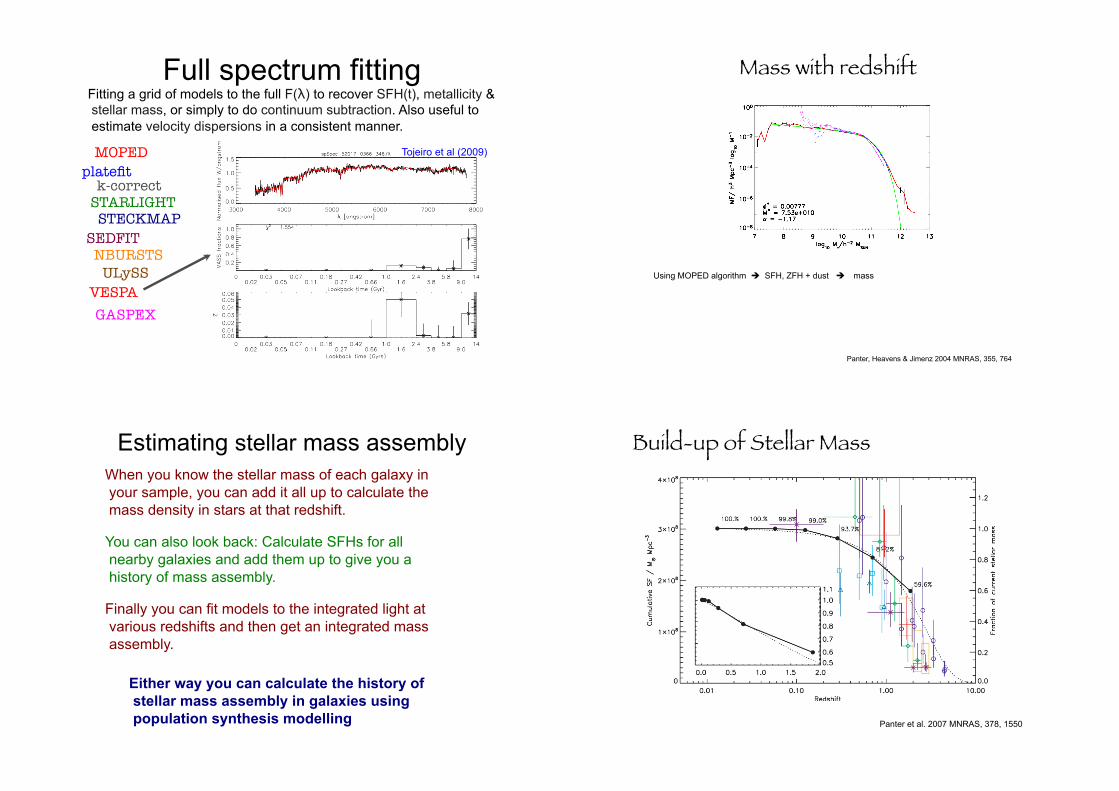
The SFH of the Universe
Panter et al. 2007 MNRAS, 378, 1550
Downsizing
Panter et al. 2007 MNRAS, 378, 1550
Emission-lines!
Tremonti et al. 2004 ApJ, 613, 989 Tremonti et al. 2004 ApJ, 613, 989

mass-metallicity relation
Tremonti et al. 2004 ApJ, 613, 989
Relation between stellar mass, in units
of solar masses, and gas-phase
oxygen abundance for 53,400 star-forming galaxies in the SDSS
The Mass-metallicity relation & the transition mass.!
Tremonti et al. 2004 ApJ, 613, 989; Brinchmann et al. 2008 A&A, 485, 657
Kauffmann et al. 2003 MNRAS, 341, 54
data ! models ! physical parameters
Brinchmann 2009 arXiv:0910.1533v1