Lecture Atmospheric Physics Contents: - IUP

Lecture Atmospheric Physics University of Bremen

Master of Environmental Physics WS 2004 / 2005

Björn-Martin Sinnhuber

room W3080, tel. 8958 [email protected]

Contents: 1. Survey of the Atmosphere

Some Basic Physics

2. Radiation in the Atmosphere Gree House Effect and Climate Change

3. Atmospheric Thermodynamics The Role of Water Vapour and Clouds

4. Dynamics of the Atmosphere

Sinnhuber: Atmospheric Physics - 2 - University of Bremen, WS 2004 / 2005

The Rules of the Game: Lectures:

• 13 lectures, every Wednesday • one “rapporteur” gives brief summary from last

lecture

Exercises: • 10 exercises • will be distributed in the lecture • will have to be submitted on the next Tuesday

(6 days to work on it...) • will be returned and discussed on the next day

in the tutorial after the lecture • credits: 10 x 10 = 100

Exam: • prerequisite to take part in the exam:

o at least 75 credits from exercises o acted at least once as rapporteur

• 2 hours written exam in the first or second week after the end of lectures


Literature for the Lecture English Books: Houghton, J.T., The physics of atmospheres, Cambridge University Press, 1977, ISBN 0 521 29656 0 Wallace, John M. and Peter V. Hobbs, Atmospheric Science, Academic Press, 1977, ISBN 0-12-732950-1 Deutsche Bücher: Roedel, Walter, Physik unserer Umwelt, Die Atmosphäre, Springer Verlag, 1992, ISBN 3-540-54285-X Script: Environmental Physics I, WS 2002/2003, Klaus Künzi and Stefan Bühler, Institute of Environmental Physics, University of Bremen, Bremen; Germany


Schematic Overview

Cosmic Radiation Sun Extraterrestrial Effects

Earth surface: Land, Orography, Albedo, Ocean and

Ocean Dynamics

RadiationAbsorption and

Emission Green House

Chemistry Photolysis

Trace Species (special course)

Water Thermodynamics

Clouds Precipitation

Stability

Dynamics


Planetary Atmospheres

Planet Gravitation (relative)

Temperature at Surface

[K]

SurfacePressure [103 hPa]

Composition

Venus 0.91 700 100 CO2 > 90%

Earth 1 290 1 N2

(~ 78 %) O2

(~ 21 %)

Mars 0.38 210 0.01 CO2

(> 80 %)

• Earth’s atmosphere is unique in pressure, temperature and atmospheric composition


Origin of the Atmosphere

• at the time of formation (4.5 x 109 years ago),

earth had no or little atmosphere

• the atmosphere was formed from volatile

emissions from the interior of the earth

(volcanic activity)

• volcanic emissions are roughly 85% H2O, 10%

CO2, and a few per cent sulphur compounds


Atmospheric Composition Today

Constituent Molecular Weight [g / mol]

Content (fraction of molecules)

Nitrogen (N2) 28.016 0.7808 Oxygen (O2) 32.00 0.2095 Argon (Ar) 39.94 0.0093 Water vapour (H2O) 18.02 0 - 0.04 Carbon Dioxide (CO2) 44.01 365 ppm Neon (Ne) 20.18 18 ppm Helium (He) 4.00 5 ppm Krypton (Kr) 83.7 1 ppm Hydrogen (H2) 2.02 0.5 ppm Ozone (O3) 48.00 0 - 12 ppm Air

≈29

1

1·10-6 = 1 ppm (part per million) 1·10-9 = 1 ppb (part per billion) 1·10-12 = 1 ppt (part per trillion)


Water Vapour in Planetary Atmospheres

• Earth is the only planet in the solar system

where water can exist in all three phases. • Most of the water emitted by volcanoes in

Earth’s history is missing (99%) • Only a very small fraction of the water is in the

atmosphere (97% in oceans, 2.4% in ice, 0.6% in underground fresh water, 0.02% in lakes and rivers, and 0.001% the atmosphere)

Water Vapor Pressure [10-1 Nm-1]

Ice

Liquid Water

Vapor

Venus Earth Mars

[K]

T


Oxygen and Life There are at least two possible sources fro oxygen in the atmosphere: Photodissociation of water:

222 OH2UVOH2 +→+ Photosynthesis by living organisms:

2

MatterOrganic

22 ),,(lightvisible2 OOHCCOOH +→++43421


The Carbon Budget • in photosynthesis, carbon is incorporated into

organic compounds • a small part of this organic matter is not

oxidized, but fossilized in shales or fossil fuels • 90% of the O2 produced by photosynthesis is

stored in the earth’s crust in oxides such as FeO3 or carbonate compounds such as CaCO3, Fe2O3, or MgCO3

• the carbonates are the main sink of atmospheric CO2

Substance Fraction [%]

Rocks 71 Shales 29 Ocean, dissolved CO2 0.1 Oil, gas, coal 0.03 Atmosphere (CO2) 0.003 Biosphere 7x10-5


Inputs / Outputs to the Atmosphere

• Input from volcanic activity • Input from meteorites • Exchange with Biosphere • Exchange with Hydrosphere • Loss to outer space and solid earth


Impact of Biosphere

• The Earth’s atmosphere is far away from the equilibrium expected for a planet without life.

• The disequilibrium is sustained by permanent emissions and adsorptions of species by the biosphere.

• Many feedback mechanisms are known through which the atmosphere is kept in its current state

• Provokingly, the atmosphere can be seen as part of the biosphere (Gaia hypothesis)


Anthropogenic Impacts Humankind is changing atmospheric composition by

• burning of fossil fuels which has a direct impact on CO2 concentrations

• emissions of trace species that alter

atmospheric chemistry in many ways • emission of trace species that alter the

radiative properties of the atmosphere directly or indirectly (cloud formation or change)


The Atmosphere in Perspective

The atmosphere

• is exceedingly thin • contains only a minute fraction of the Earth’s

mass (0.025%), even for its main constituents • Lithosphere (the earth’s crust), Hydrosphere

(water on or above the earth’s surface) and Biosphere (all animal and plant life) act as huge reservoirs for atmospheric constituents


Vertical Structure of the Atmosphere


Vertical Structure of the Atmosphere Classification according to T-profile:

• Troposphere • Stratosphere • Mesosphere • Thermosphere • Exosphere

Boundaries between layers are called “-pause”; most important here: the tropopause Tropopause varies with season, latitude, temperature and pressure systems Different tropopause definitions based on T, O3, potential temperature, H2O, or combinations of the above. Classification according to mixing:

• Homosphere • Heterosphere


Ideal Gas Assumptions:

• ensemble of individual molecules • no interaction apart from collision • no chemical reactions • no appreciable volume of individual molecules

State properties of a gas: p, T, V, and n Equation of state for the ideal gas:

NkTpVnRTpV == or

p = pressure, V = volume, n = number of moles, N = number of molecules, R = universal gas constant,

k = Boltzman constant, T = temperature All gases act as ideal gases at very low pressure; to good approximation, gases in the atmosphere can be treated as ideal gases with the exception of water vapour (phase changes)


Mixtures of Ideal Gases Dalton’s law: The pressure exerted by a mixture of perfect gases is the sum of the pressures exerted by the individual gases occupying the same volume alone or

BA ppp += Mole fraction: The mole fraction of a gas X in a mixture is the number of moles of X molecules present (nX) as a fraction of the total number of moles of molecules (n) in the sample:

... with +++== CBAX

X nnnnn

nx

Partial pressure: The partial pressure of a gas in a mixture is defined as the product of mole fraction of this gas and total pressure of the gas:

pxp Xx =


Abundance Units in Atmospheric Science

quantity symbol units

number of molecules

N mol = 6.022 x1023

number density n particles / m3 mass density ρ kg / m3

volume mixing ratio

µ ppmV = 10-6 ppbV = 10-9 pptV = 10-12

mass mixing ratio

µ ppmm =10-6 ppbm =10-9 pptm = 10-12

column abundance

molec/cm2

or DU = 10-3 cm at STP


Excursion: Ideal Gas Law The ideal gas law can be expressed in molecules or moles:

NkTpVnRTpV == or R or R* = Universal gas constant = 8.314 J mol-1 K-1 k = Boltzmann’s constant = 1.381 10-23 J molec-1 K-1

NA = Avogadro’s number = 6.022 1023 mol-1 R = NA k Number density:

kTp

VN =

Mass density:

RTpM

kTNpM

kTpm

VNm

Vm x

A

xxx =====ρ

mx = Mass of one molecule x, Mx molar mass of x In some books, individual gas constants are defined for each gas:

xx M

RR =


Virtual Temperature: Problem: The molecular weight of air is not constant, but changes with water vapour pressure Solution: Define a fictitious virtual temperature, that dry air must have to have the same density that the moist air has at a given pressure. The density of moist air is

''2vd

OHd

Vmm ρρρ +=

+=

md = mass of dry air, mH2O mass of water vapour where ρd’ is the density dry air would have if it would occupy the volume alone. From the ideal gas equation, the partial pressures of water vapour e and dry air pd can be derived:

OHvv MTRp 2/'ρ=

airdd MTRp /'' ρ=

and total pressure is vd ppp += '


Inserting into the equation for the density

RTMp

TRppM OHvvd 2)(

+−

=ρ

−−= )1(1 ερ

pp

RTpM vd

with

622.02 ==

d

OH

MMε

If we now define a virtual Temperature Tv as

)1)(/(1 ε−−=

ppTT

vv

we can write the equation of state for moist air in the ideal gas form using the molecular weight of dry air:

d

v

MTR

pρ

=


Moist air is less dense than dry air, therefore the virtual temperature is always larger than the real temperature (the difference is usually small). In the future, virtual temperature will be used throughout without special notice.

Note that we can write the virtual temperature also as

( )qTqTTv 608.0111 +=

−+=

εε

with q being the specific humidity:

vd

v

dv

vv

ppp

qε

ερρ

ρρρ

+=

+==


Hydrostatic Equation

dzgdp ⋅⋅−= ρ

Ideal gas

TRnVp ⋅=⋅

Definition of density:

TRpM

VMn

⋅⋅=⋅=ρ

Insert:

dzTRgMpdp ⋅

⋅⋅⋅−=

Integrate:

⋅

⋅⋅−= zTRgMpp exp0

p = pressure M = molar air mass,

g = gravitational acceleration, R = universal gas constant, T = temperature, z = height,

V = volume, ρ = density


Geopotential Definition: The Geopotential Φ of any point in the atmosphere is the work that most be done against the earth’s gravitational field in order to raise a mass of 1 kg from sea level to the point.

gdzmgdzd ==Φ and setting Φ(0) = 0

∫=Φz

dzzgz0

)()(

• Φ does not depend on the path used to move

a mass from the sea surface to a point • the differences in geopotential between two

points ΦB - ΦA is the work in the gravitational field needed to move a mass of 1 kg from point A to point B

The geopotential depends on altitude as a result of the distance dependence of the gravitational force.


The geopotential also depends on latitude mainly because of the flattening of earth at the poles and the latitudinal dependence of the centrifugal force. From the geopotential, we can also define a Geopotential Height

∫=Φ=z

dzzggg

zZ000

)(1)(

where g0=9.8 ms-2 is the globally averaged gravitational acceleration at sea surface level. Geopotential height is used as vertical coordinate in most atmospheric applications where energy plays an important role.


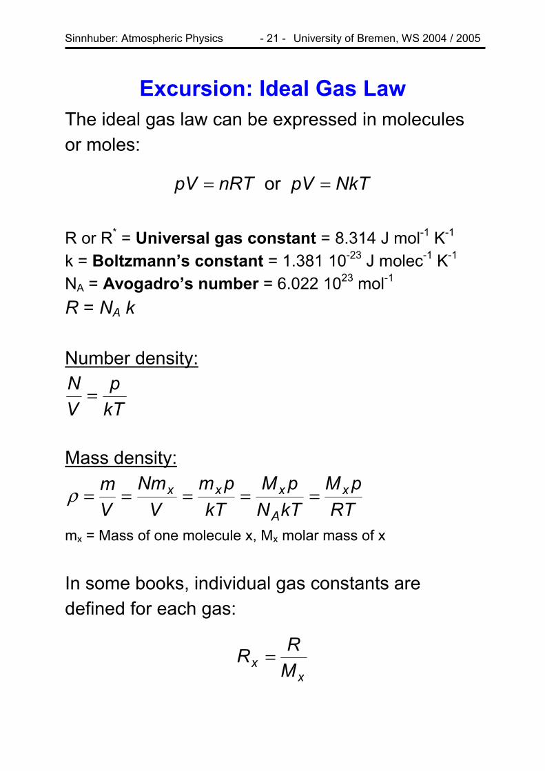
Hypsometric Equation From the definition of the geopotential

gdzd =Φ

and the hydrostatic equation dzgdp ⋅⋅−= ρ

we get

dppTRdpd vd−=−=Φ

ρ1

Then integration leads to

∫−=Φ−Φ2

1

12

p

p

vd dppT

R

and dividing by g0 we find for the difference between two geopotential heights

∫=−1

2012

p

p

vd dppT

gR

ZZ

If we can describe the temperature between p1 and

p2 by a (constant) mean temperature vT then


∫=−1

2012

p

p

vd

pdp

gTR

ZZ

integrating from p2 to p1 gives:

=−

2

1

012 ln

pp

gTR

ZZ vd

This is the so-called hypsometric equation. It states that the thickness of a layer between two pressure surfaces is proportional to the (mean) temperature of this layer.


Scale Height The factor in the exponent in the hydrostatic equation

⋅

⋅⋅−= zTRgMpp exp0

has the units of inverse length and is called the Scale Height:

MgRTz =0

Often, the hydrostatic equation is expressed as

( )00 /exp zzpp −= The scale height is the height at which pressure is reduced by a factor of e (2.718); for the atmosphere as a whole it is about 8km which corresponds to a reduction to half the value at 5.5 km. The scale height depends on M and thus is different for different species; also, it depends on T and thereby altitude.


Examples for scale heights: Different Planets: Planet name

Major atmospheric constituent

M [g]

g0

[m/s2]Tsurfac

e [K] H [km]

Venus CO2 44 8.9 700 14.9 Earth N2,O2 29 9.8 270 7.9 Mars CO2 44 3.7 210 10.6 Jupiter H2 2 26.2 160 25.3

Different Species

Species Molecular Mass M [g]

Scale height H in [km]

Argon (Ar) 40 21 Nitrogen (N2) 28 30 Atomic Oxygen (O) 16 54 Atomic Hydrogen (H) 1 850


Isobaric Atmosphere It is sometimes useful to imagine an atmosphere where everything is brought to surface pressure (and temperature). In such a model atmosphere, the density is constant and equal to the surface density ρ0. The thickness of this atmosphere can be derived from evaluating the total mass

00

000

00 )/exp()(

z

dzzzdzzM

ρ

ρρ

=

−== ∫∫∞∞

and is identical to the scale height z0. This relation is sometimes used to define a scale height for constituents with arbitrary vertical profiles c(z):

∫∞

=00

0 )(1 dzzcc

z

where c0 is the concentration at the surface.


Distributions of Speed The Maxwell-Boltzmann distribution of speed is

kTmvx

xekT

mvf 2/2/1

2

2)( −

=

π

The Maxwell distribution of speeds is

kTmvevkT

mvf 2/22/3 2

24)( −

=

ππ


Gas Velocities The most probable speed c* is the speed corresponding to the maximum of the distribution:

2/12*

=

mKTc

The mean speed in contrast is the weighted speed

2/18

=

mKTc

π

which again is slightly different from the root mean square speed

2/13

=

mKTc

Speed depends on mass, typical values for mean speed at 25°C are N2 : 475 m/s He : 1256 m/s


Escape Velocity A moving body (in this case: a molecule) can leave the earth’s gravitational field if its kinetic energy is larger than the potential energy needed to overcome the gravitational field. It depends only on altitude and at 500 km is of the order of 11 km s-1. If the speed of a molecule is high enough, and at the same time the mean free path is long enough, it may leave the atmosphere. The speed depends on temperature and mass, the mean free path on density. Typical values for mean free path are 200 km: 200m 100 km: 15 cm 0 km: 0.06µm Below 100 km (Homosphere), collisions between molecules are so frequent that all constituents are well mixed and no separation is possible. Above that altitude, the different scale heights come into effect (Heterosphere).


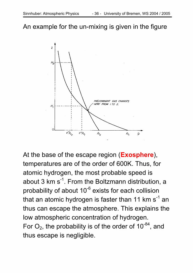
An example for the un-mixing is given in the figure

At the base of the escape region (Exosphere), temperatures are of the order of 600K. Thus, for atomic hydrogen, the most probable speed is about 3 km s-1. From the Boltzmann distribution, a probability of about 10-6 exists for each collision that an atomic hydrogen is faster than 11 km s-1 an thus can escape the atmosphere. This explains the low atmospheric concentration of hydrogen. For O2, the probability is of the order of 10-84, and thus escape is negligible.


Ionosphere At high altitudes (> 60 km), the relative density of ions and electrons increases as a result of ionisation of air molecules by solar X-ray and UV radiation. High energy cosmic rays also contribute to ionisation. This layer is sometimes also called Heaviside Layer. Ionisation increases with altitude as a result of

• increased mean free path => increased life time

• increased radiation The free electrons in the Ionosphere have an impact on radio communication by reflecting or absorbing radio waves and also act a s a Faraday cage against charged particles. Charged particles are also produced in the atmosphere by other processes:

• radioactive decay of substances within the earth’s crust

• charge separation within clouds


The free electrons make the ionosphere conducting, a so-called plasma. For a given electron density we can calculate the plasma frequency f , this results in the fact that the plasma becomes a reflector for all electromagnetic waves with frequencies pff <

Nconstm

eNfp ==0

12 επ

with the 3109 −⋅≈const , pf in [MHz] and the electron density N in [cm-3], m the mass of the electron and ε0 the permittivity in vacuum. Therefore for an electron density of

35103 −⋅= cmN we find a plasma frequency MHzfp 5≈

Region Altitude [km] Electron density [cm3]

(typical, order of magnitude)

D < 90 103-104 E 90 - 140 105 F1 F2

> 140 Maximum of 106 in the region of 250 - 500 km


Layers in the Ionosphere Three regions can be distinguished:

• D-layer (absorbing due to collisions with uncharged molecules)

• E-layer (density large enough that positive ions drift with the neutral constituents while electrons move along magnetic field lines and thus charges are separated, currents flow and voltages are induced)

• F-layer (long mean free path, structure determined by fields induced from E-region)


Diurnal cycle of the Ionosphere At night, the electron density decreases, and the D-layer disappears. The F1 and F2-layers combine, and in the highest atmosphere the diurnal variation is small:

The absence of the absorbing D-layer has a large impact on radio communication that at night can suffer from reflections at the F-layer in the AM band whereas long range short wave communications work better at night. The ionosphere also responds strongly to solar eruptions.


Extract from http://www.spaceweather.com/ What's Up in Space -- 29 Oct 2003

AURORAS NOW! The coronal mass ejection described below has reached Earth (at approximately 0630 UT on Oct. 29th) and triggered a strong geomagnetic storm. This storm is ongoing! Red and green Northern

Lights have been spotted as far south as Bishop, California. Stay tuned for updates.

EXTREME SOLAR ACTIVITY: One of the most powerful solar flares in years erupted from giant sunspot 486 this morning at approximately 1110 UT. The blast measured X17 on the Richter scale of solar flares. As a result of the explosion, a severe S4-class solar radiation storm is underway. Click here to learn how such storms can affect our planet. The explosion also hurled a coronal mass ejection (CME) toward Earth. When it left the sun, the cloud was traveling 2125 km/s (almost 5 million mph). This CME could trigger bright auroras when it sweeps past our planet perhaps as early as tonight.

Above: This SOHO coronagraph image captured at 12:18 UT shows the coronal mass ejection of Oct. 28th billowing directly toward Earth. Such clouds are called halo CMEs. The many speckles are solar protons striking the coronagraph's CCD camera. See the complete movie.

Where will the auroras appear? High-latitude sites such as New Zealand, Scandinavia, Alaska, Canada and US northern border states from Maine to Washington are favored, as usual, but auroras could descend to lower latitudes when the CME pictured above sweeps past Earth.

Right: Photographer Lance Taylor of Alberta, Canada, spotted these vivid Northern Lights on Oct. 21st. [gallery]

Not all CMEs trigger auroras. Several, for instance, have swept past Earth in recent days without causing widespread displays. It all depends on the orientation of tangled magnetic fields within the electrified cloud of gas. The incoming CME is no exception. It might cause auroras, or it might not. We will find out when it arrives.


Probing the Ionosphere The electron density in the Ionosphere can be studied from the ground (and from space) by emitting radio signals at different frequencies and measuring the time lag of the reflected signal (Ionosonde):

To reach higher altitudes, the frequency is increased. Absorption in the D-layer can not be studied in this way.


Magnetosphere Above 500 km, collisions are infrequent and the magnetic field determines the motion of charged particles. Earth’s magnetic field is approximately a dipole with 11° inclination to the rotation axis. Solar wind distorts the magnetic field:

Solar outbursts impact the magnetic field and inject high energy particles into the lower ionosphere, which gives rise to brilliant auroral displays. The magnetic field provides an important shield from solar wind.


Van Allen Belts Charged particles that entered the magnetosphere experience a force perpendicular to their velocity and the magnetic field and travel around magnetic field lines from pole to pole (1s) and rotate around the earth:

Close to the poles the particles can reach lower altitudes (80 - 150 km) where they can ionise air molecules which then emit light when recombining.


Aurora Coloured lights in the sky at night in polar latitudes, mostly in an oval between 15° and 30° from the magnetic poles. Aurora borealis = aurora in the Arctic Aurora australis = aurora in the Antarctic Source: Atomic and molecular emissions from oxygen and nitrogen caused by ionisation by fast charged particles in the ionosphere. The particles do not originate from the solar wind but are produced by it.


Earth in Space

• Earth’s orbit around the sun is slightly elliptic (149.6x106 km - 152x106 km)

• Earth’s ecliptic is 23.5° • seasons are result of ecliptic, not elliptic orbit • during summer, there is polar day polewards of

the arctic cycle, depending on date • during winter, the pole is without solar

illumination (polar night • twice per year, there is equinox (21.3. and

23.9.)


• in the tropics, the sun is in the zenith twice per year

• at solstice, the sun is in the zenith over the Tropic of Capricorn (December) or the Tropic of Cancer (June)

• day length varies slightly in the tropics but very much in high latitudes

from :http://www.bath.ac.uk/~absmaw/Facade/sunlight_01.pdf

Lecture Atmospheric Physics Contents: - IUP

Documents

Transcript of Lecture Atmospheric Physics Contents: - IUP