© aSup-2007 Central Tendency 1 CENTRAL TENDENCY Mean, Median, and Mode.
Measures of Central Tendency Sampling Distributions The Sampling Distribution of the Mean The Sampling Distribution of the M
Lecture 9: Measures of Central Tendency andSampling Distributions
Assist. Prof. Dr. Emel YAVUZ DUMAN
Introduction to Probability and StatisticsIstanbul Kultur UniversityFaculty of Engineering
Measures of Central Tendency Sampling Distributions The Sampling Distribution of the Mean The Sampling Distribution of the M
Outline
1 Measures of Central Tendency
2 Sampling DistributionsPopulation and Sample. Statistical InferenceSampling With and Without ReplacementRandom Samples
3 The Sampling Distribution of the Mean
4 The Sampling Distribution of the Mean: Finite Population
Measures of Central Tendency Sampling Distributions The Sampling Distribution of the Mean The Sampling Distribution of the M
Introduction
A measure of central tendency is a single value that attempts todescribe a set of data by identifying the central position within thatset of data.
Measures of Central Tendency Sampling Distributions The Sampling Distribution of the Mean The Sampling Distribution of the M
Introduction
A measure of central tendency is a single value that attempts todescribe a set of data by identifying the central position within thatset of data. As such, measures of central tendency are sometimescalled measures of central location.
Measures of Central Tendency Sampling Distributions The Sampling Distribution of the Mean The Sampling Distribution of the M
Introduction
A measure of central tendency is a single value that attempts todescribe a set of data by identifying the central position within thatset of data. As such, measures of central tendency are sometimescalled measures of central location. They are also classed assummary statistics.
Measures of Central Tendency Sampling Distributions The Sampling Distribution of the Mean The Sampling Distribution of the M
Introduction
A measure of central tendency is a single value that attempts todescribe a set of data by identifying the central position within thatset of data. As such, measures of central tendency are sometimescalled measures of central location. They are also classed assummary statistics. The mean (often called the average) is mostlikely the measure of central tendency that you are most familiarwith, but there are others, such as the median and the mode.The mean, median and mode are all valid measures of centraltendency, but under different conditions, some measures of centraltendency become more appropriate to use than others.
Measures of Central Tendency Sampling Distributions The Sampling Distribution of the Mean The Sampling Distribution of the M
Introduction
A measure of central tendency is a single value that attempts todescribe a set of data by identifying the central position within thatset of data. As such, measures of central tendency are sometimescalled measures of central location. They are also classed assummary statistics. The mean (often called the average) is mostlikely the measure of central tendency that you are most familiarwith, but there are others, such as the median and the mode.The mean, median and mode are all valid measures of centraltendency, but under different conditions, some measures of centraltendency become more appropriate to use than others. In thefollowing, we will look at the mean, mode and median, and learnhow to calculate them and under what conditions they are mostappropriate to be used.
Measures of Central Tendency Sampling Distributions The Sampling Distribution of the Mean The Sampling Distribution of the M
Mean (Arithmetic)
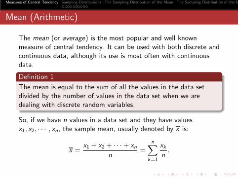
The mean (or average) is the most popular and well knownmeasure of central tendency.
Measures of Central Tendency Sampling Distributions The Sampling Distribution of the Mean The Sampling Distribution of the M
Mean (Arithmetic)
The mean (or average) is the most popular and well knownmeasure of central tendency. It can be used with both discrete andcontinuous data, although its use is most often with continuousdata.
Definition 1
The mean is equal to the sum of all the values in the data setdivided by the number of values in the data set when we aredealing with discrete random variables.
So, if we have n values in a data set and they have valuesx1, x2, · · · , xn, the sample mean, usually denoted by x is:
x =x1 + x2 + · · ·+ xn
n=
n∑k=1
xkn.
Measures of Central Tendency Sampling Distributions The Sampling Distribution of the Mean The Sampling Distribution of the M
Finding the Mean from Tables
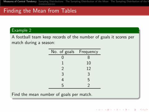
Example 2
A football team keep records of the number of goals it scores permatch during a season:
No. of goals Frequency
0 81 102 123 34 55 2
Find the mean number of goals per match.
Measures of Central Tendency Sampling Distributions The Sampling Distribution of the Mean The Sampling Distribution of the M
Finding the Mean from Tables
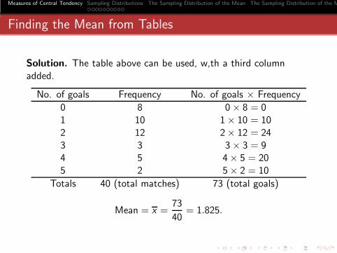
Solution. The table above can be used, w,th a third columnadded.
No. of goals Frequency No. of goals × Frequency
0 8 0× 8 = 01 10 1× 10 = 102 12 2× 12 = 243 3 3× 3 = 94 5 4× 5 = 205 2 5× 2 = 10
Totals 40 (total matches) 73 (total goals)
Mean = x =73
40= 1.825.
Measures of Central Tendency Sampling Distributions The Sampling Distribution of the Mean The Sampling Distribution of the M
Median
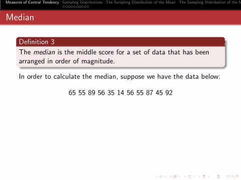
Definition 3
The median is the middle score for a set of data that has beenarranged in order of magnitude.
Measures of Central Tendency Sampling Distributions The Sampling Distribution of the Mean The Sampling Distribution of the M
Median
Definition 3
The median is the middle score for a set of data that has beenarranged in order of magnitude.
In order to calculate the median, suppose we have the data below:
65 55 89 56 35 14 56 55 87 45 92
Measures of Central Tendency Sampling Distributions The Sampling Distribution of the Mean The Sampling Distribution of the M
Median
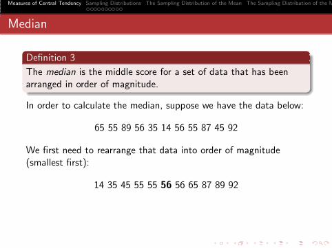
Definition 3
The median is the middle score for a set of data that has beenarranged in order of magnitude.
In order to calculate the median, suppose we have the data below:
65 55 89 56 35 14 56 55 87 45 92
We first need to rearrange that data into order of magnitude(smallest first):
14 35 45 55 55 56 56 65 87 89 92
Measures of Central Tendency Sampling Distributions The Sampling Distribution of the Mean The Sampling Distribution of the M
Median
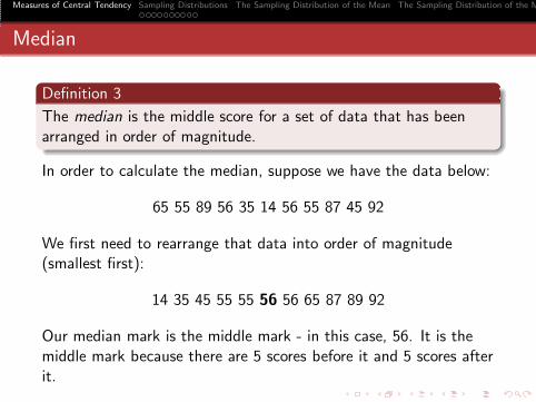
Definition 3
The median is the middle score for a set of data that has beenarranged in order of magnitude.
In order to calculate the median, suppose we have the data below:
65 55 89 56 35 14 56 55 87 45 92
We first need to rearrange that data into order of magnitude(smallest first):
14 35 45 55 55 56 56 65 87 89 92
Our median mark is the middle mark - in this case, 56. It is themiddle mark because there are 5 scores before it and 5 scores afterit.
Measures of Central Tendency Sampling Distributions The Sampling Distribution of the Mean The Sampling Distribution of the M
Median
This works fine when you have an odd number of scores, but whathappens when you have an even number of scores?
Measures of Central Tendency Sampling Distributions The Sampling Distribution of the Mean The Sampling Distribution of the M
Median
This works fine when you have an odd number of scores, but whathappens when you have an even number of scores?What if you hadonly 10 scores?
Measures of Central Tendency Sampling Distributions The Sampling Distribution of the Mean The Sampling Distribution of the M
Median
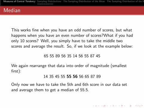
This works fine when you have an odd number of scores, but whathappens when you have an even number of scores?What if you hadonly 10 scores? Well, you simply have to take the middle twoscores and average the result.
Measures of Central Tendency Sampling Distributions The Sampling Distribution of the Mean The Sampling Distribution of the M
Median
This works fine when you have an odd number of scores, but whathappens when you have an even number of scores?What if you hadonly 10 scores? Well, you simply have to take the middle twoscores and average the result. So, if we look at the example below:
65 55 89 56 35 14 56 55 87 45
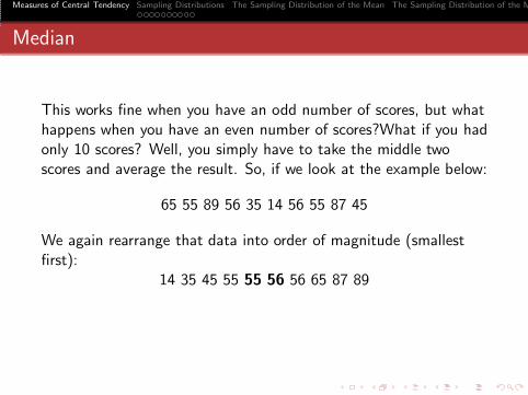
We again rearrange that data into order of magnitude (smallestfirst):
14 35 45 55 55 56 56 65 87 89
Measures of Central Tendency Sampling Distributions The Sampling Distribution of the Mean The Sampling Distribution of the M
Median
This works fine when you have an odd number of scores, but whathappens when you have an even number of scores?What if you hadonly 10 scores? Well, you simply have to take the middle twoscores and average the result. So, if we look at the example below:
65 55 89 56 35 14 56 55 87 45
We again rearrange that data into order of magnitude (smallestfirst):
14 35 45 55 55 56 56 65 87 89
Only now we have to take the 5th and 6th score in our data setand average them to get a median of 55.5.
Measures of Central Tendency Sampling Distributions The Sampling Distribution of the Mean The Sampling Distribution of the M
Median
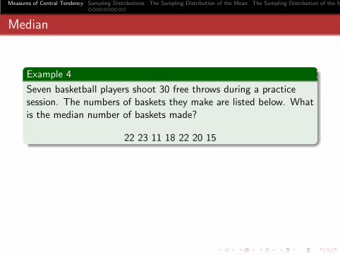
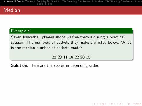
Example 4
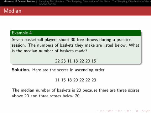
Seven basketball players shoot 30 free throws during a practicesession. The numbers of baskets they make are listed below. Whatis the median number of baskets made?
22 23 11 18 22 20 15
Measures of Central Tendency Sampling Distributions The Sampling Distribution of the Mean The Sampling Distribution of the M
Median
Example 4
Seven basketball players shoot 30 free throws during a practicesession. The numbers of baskets they make are listed below. Whatis the median number of baskets made?
22 23 11 18 22 20 15
Solution. Here are the scores in ascending order.
11 15 18 20 22 22 23
The median number of baskets is 20 because there are three scoresabove 20 and three scores below 20.
Measures of Central Tendency Sampling Distributions The Sampling Distribution of the Mean The Sampling Distribution of the M
Example 5
Twelve members of a gym class, some in good physical conditionand some in not-so-good physical condition, see how many sit-upsthey can complete in a minute. Here are their scores.
2 3 6 10 12 12 14 15 15 15 24 25
What is the median number of sit-ups?
Solution. The median is 13, because there are six scores below 13and six scores above 13.
Measures of Central Tendency Sampling Distributions The Sampling Distribution of the Mean The Sampling Distribution of the M
Example 5
Twelve members of a gym class, some in good physical conditionand some in not-so-good physical condition, see how many sit-upsthey can complete in a minute. Here are their scores.
2 3 6 10 12 12 14 15 15 15 24 25
What is the median number of sit-ups?
Solution. The median is 13, because there are six scores below 13and six scores above 13. Note that the median does not necessarilyhave to be an existing score.
Measures of Central Tendency Sampling Distributions The Sampling Distribution of the Mean The Sampling Distribution of the M
Example 5
Twelve members of a gym class, some in good physical conditionand some in not-so-good physical condition, see how many sit-upsthey can complete in a minute. Here are their scores.
2 3 6 10 12 12 14 15 15 15 24 25
What is the median number of sit-ups?
Solution. The median is 13, because there are six scores below 13and six scores above 13. Note that the median does not necessarilyhave to be an existing score. In this case, no one completedexactly 13 sit-ups.
Measures of Central Tendency Sampling Distributions The Sampling Distribution of the Mean The Sampling Distribution of the M
Mode
Definition 6
The mode is the most frequently occurring value in a set of values.
Measures of Central Tendency Sampling Distributions The Sampling Distribution of the Mean The Sampling Distribution of the M
Mode
Definition 6
The mode is the most frequently occurring value in a set of values.
The mode is the most frequent score in our data set.
Measures of Central Tendency Sampling Distributions The Sampling Distribution of the Mean The Sampling Distribution of the M
Mode
Definition 6
The mode is the most frequently occurring value in a set of values.
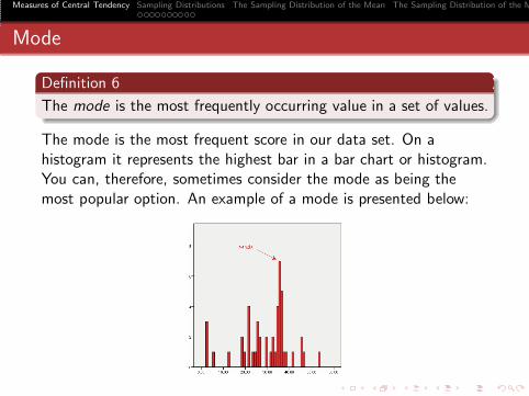
The mode is the most frequent score in our data set. On ahistogram it represents the highest bar in a bar chart or histogram.
Measures of Central Tendency Sampling Distributions The Sampling Distribution of the Mean The Sampling Distribution of the M
Mode
Definition 6
The mode is the most frequently occurring value in a set of values.
The mode is the most frequent score in our data set. On ahistogram it represents the highest bar in a bar chart or histogram.You can, therefore, sometimes consider the mode as being themost popular option.
Measures of Central Tendency Sampling Distributions The Sampling Distribution of the Mean The Sampling Distribution of the M
Mode
Definition 6
The mode is the most frequently occurring value in a set of values.
The mode is the most frequent score in our data set. On ahistogram it represents the highest bar in a bar chart or histogram.You can, therefore, sometimes consider the mode as being themost popular option. An example of a mode is presented below:
Measures of Central Tendency Sampling Distributions The Sampling Distribution of the Mean The Sampling Distribution of the M
Mode
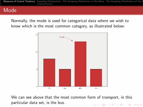
Normally, the mode is used for categorical data where we wish toknow which is the most common category, as illustrated below:
We can see above that the most common form of transport, in thisparticular data set, is the bus.
Measures of Central Tendency Sampling Distributions The Sampling Distribution of the Mean The Sampling Distribution of the M
Mode
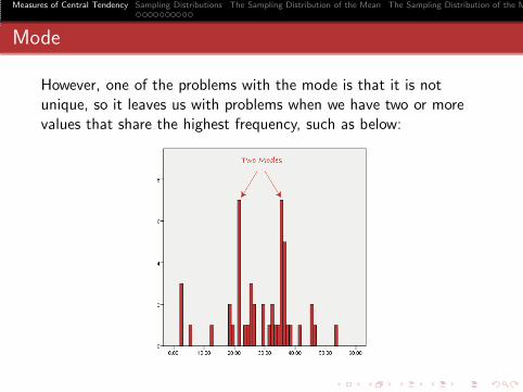
However, one of the problems with the mode is that it is notunique, so it leaves us with problems when we have two or morevalues that share the highest frequency, such as below:
Measures of Central Tendency Sampling Distributions The Sampling Distribution of the Mean The Sampling Distribution of the M
Mode
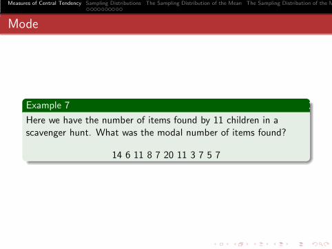
Example 7
Here we have the number of items found by 11 children in ascavenger hunt. What was the modal number of items found?
14 6 11 8 7 20 11 3 7 5 7
Measures of Central Tendency Sampling Distributions The Sampling Distribution of the Mean The Sampling Distribution of the M
Mode
Solution. If there are not too many numbers, a simple list ofscores will do.
Measures of Central Tendency Sampling Distributions The Sampling Distribution of the Mean The Sampling Distribution of the M
Mode
Solution. If there are not too many numbers, a simple list ofscores will do. However, if there are many scores, you will need toput the scores in order and then create a frequency table.
Measures of Central Tendency Sampling Distributions The Sampling Distribution of the Mean The Sampling Distribution of the M
Mode
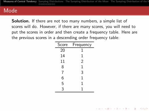
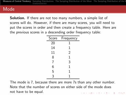
Solution. If there are not too many numbers, a simple list ofscores will do. However, if there are many scores, you will need toput the scores in order and then create a frequency table. Here arethe previous scores in a descending order frequency table:
Score Frequency
20 114 111 28 17 36 15 13 1
Measures of Central Tendency Sampling Distributions The Sampling Distribution of the Mean The Sampling Distribution of the M
Mode
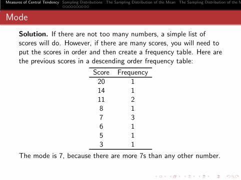
Solution. If there are not too many numbers, a simple list ofscores will do. However, if there are many scores, you will need toput the scores in order and then create a frequency table. Here arethe previous scores in a descending order frequency table:
Score Frequency
20 114 111 28 17 36 15 13 1
The mode is 7, because there are more 7s than any other number.
Measures of Central Tendency Sampling Distributions The Sampling Distribution of the Mean The Sampling Distribution of the M
Mode
Solution. If there are not too many numbers, a simple list ofscores will do. However, if there are many scores, you will need toput the scores in order and then create a frequency table. Here arethe previous scores in a descending order frequency table:
Score Frequency
20 114 111 28 17 36 15 13 1
The mode is 7, because there are more 7s than any other number.Note that the number of scores on either side of the mode doesnot have to be equal.

Measures of Central Tendency Sampling Distributions The Sampling Distribution of the Mean The Sampling Distribution of the M
Mode
Example 8
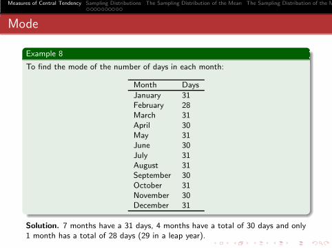
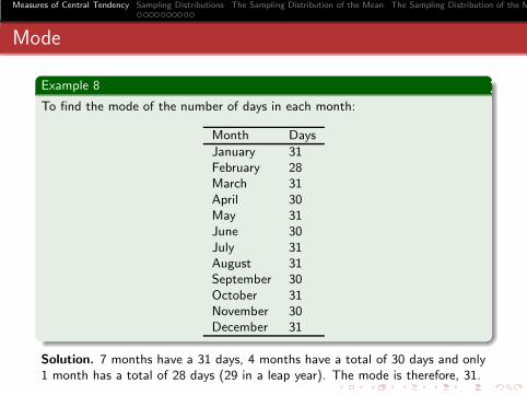
To find the mode of the number of days in each month:
Month Days
January 31February 28March 31April 30May 31June 30July 31August 31September 30October 31November 30December 31
Measures of Central Tendency Sampling Distributions The Sampling Distribution of the Mean The Sampling Distribution of the M
Mode
Example 8
To find the mode of the number of days in each month:
Month Days
January 31February 28March 31April 30May 31June 30July 31August 31September 30October 31November 30December 31
Solution. 7 months have a 31 days, 4 months have a total of 30 days and only1 month has a total of 28 days (29 in a leap year).
Measures of Central Tendency Sampling Distributions The Sampling Distribution of the Mean The Sampling Distribution of the M
Mode
Example 8
To find the mode of the number of days in each month:
Month Days
January 31February 28March 31April 30May 31June 30July 31August 31September 30October 31November 30December 31
Solution. 7 months have a 31 days, 4 months have a total of 30 days and only1 month has a total of 28 days (29 in a leap year). The mode is therefore, 31.
Measures of Central Tendency Sampling Distributions The Sampling Distribution of the Mean The Sampling Distribution of the M
Mode
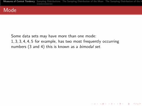
Some data sets may have more than one mode:
Measures of Central Tendency Sampling Distributions The Sampling Distribution of the Mean The Sampling Distribution of the M
Mode
Some data sets may have more than one mode:1, 3, 3, 4, 4, 5 for example, has two most frequently occurringnumbers (3 and 4) this is known as a bimodal set.
Measures of Central Tendency Sampling Distributions The Sampling Distribution of the Mean The Sampling Distribution of the M
Mode
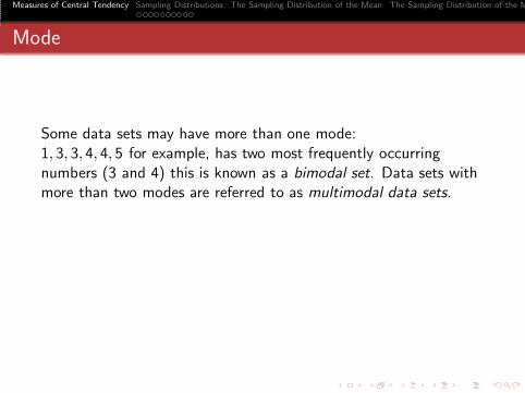
Some data sets may have more than one mode:1, 3, 3, 4, 4, 5 for example, has two most frequently occurringnumbers (3 and 4) this is known as a bimodal set. Data sets withmore than two modes are referred to as multimodal data sets.

Measures of Central Tendency Sampling Distributions The Sampling Distribution of the Mean The Sampling Distribution of the M
Mode
Some data sets may have more than one mode:1, 3, 3, 4, 4, 5 for example, has two most frequently occurringnumbers (3 and 4) this is known as a bimodal set. Data sets withmore than two modes are referred to as multimodal data sets.If a data set contains only unique numbers then calculating themode is more problematic.
Measures of Central Tendency Sampling Distributions The Sampling Distribution of the Mean The Sampling Distribution of the M
Mode
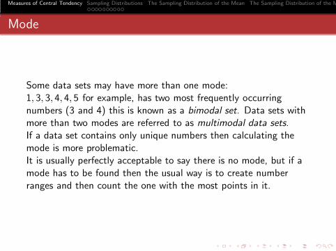
Some data sets may have more than one mode:1, 3, 3, 4, 4, 5 for example, has two most frequently occurringnumbers (3 and 4) this is known as a bimodal set. Data sets withmore than two modes are referred to as multimodal data sets.If a data set contains only unique numbers then calculating themode is more problematic.It is usually perfectly acceptable to say there is no mode, but if amode has to be found then the usual way is to create numberranges and then count the one with the most points in it.
Measures of Central Tendency Sampling Distributions The Sampling Distribution of the Mean The Sampling Distribution of the M
Mode
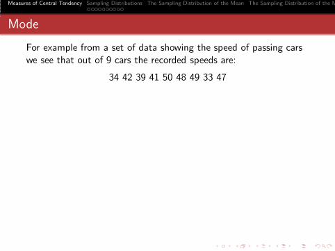
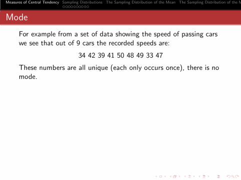
For example from a set of data showing the speed of passing carswe see that out of 9 cars the recorded speeds are:
34 42 39 41 50 48 49 33 47
Measures of Central Tendency Sampling Distributions The Sampling Distribution of the Mean The Sampling Distribution of the M
Mode
For example from a set of data showing the speed of passing carswe see that out of 9 cars the recorded speeds are:
34 42 39 41 50 48 49 33 47
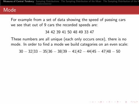
These numbers are all unique (each only occurs once), there is nomode.
Measures of Central Tendency Sampling Distributions The Sampling Distribution of the Mean The Sampling Distribution of the M
Mode
For example from a set of data showing the speed of passing carswe see that out of 9 cars the recorded speeds are:
34 42 39 41 50 48 49 33 47
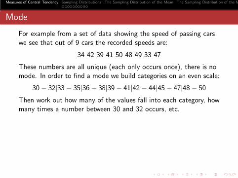
These numbers are all unique (each only occurs once), there is nomode. In order to find a mode we build categories on an even scale:
30− 32|33 − 35|36 − 38|39 − 41|42 − 44|45 − 47|48 − 50
Measures of Central Tendency Sampling Distributions The Sampling Distribution of the Mean The Sampling Distribution of the M
Mode
For example from a set of data showing the speed of passing carswe see that out of 9 cars the recorded speeds are:
34 42 39 41 50 48 49 33 47
These numbers are all unique (each only occurs once), there is nomode. In order to find a mode we build categories on an even scale:
30− 32|33 − 35|36 − 38|39 − 41|42 − 44|45 − 47|48 − 50
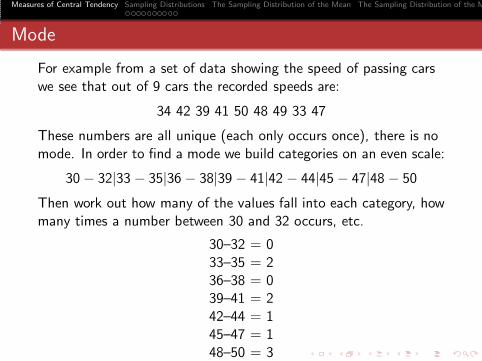
Then work out how many of the values fall into each category, howmany times a number between 30 and 32 occurs, etc.
Measures of Central Tendency Sampling Distributions The Sampling Distribution of the Mean The Sampling Distribution of the M
Mode
For example from a set of data showing the speed of passing carswe see that out of 9 cars the recorded speeds are:
34 42 39 41 50 48 49 33 47
These numbers are all unique (each only occurs once), there is nomode. In order to find a mode we build categories on an even scale:
30− 32|33 − 35|36 − 38|39 − 41|42 − 44|45 − 47|48 − 50
Then work out how many of the values fall into each category, howmany times a number between 30 and 32 occurs, etc.
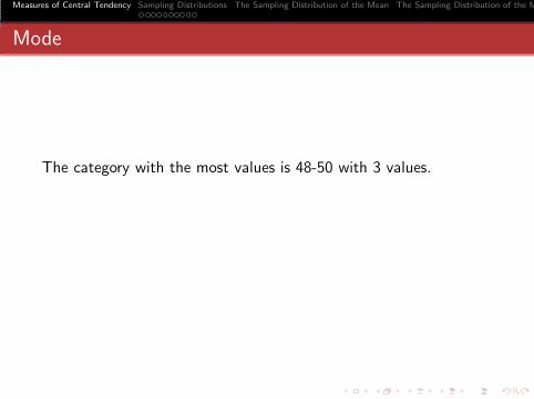
30–32 = 033–35 = 236–38 = 039–41 = 242–44 = 145–47 = 148–50 = 3
Measures of Central Tendency Sampling Distributions The Sampling Distribution of the Mean The Sampling Distribution of the M
Mode
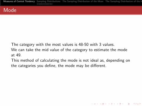
The category with the most values is 48-50 with 3 values.

Measures of Central Tendency Sampling Distributions The Sampling Distribution of the Mean The Sampling Distribution of the M
Mode
The category with the most values is 48-50 with 3 values.We can take the mid value of the category to estimate the modeat 49.
Measures of Central Tendency Sampling Distributions The Sampling Distribution of the Mean The Sampling Distribution of the M
Mode
The category with the most values is 48-50 with 3 values.We can take the mid value of the category to estimate the modeat 49.This method of calculating the mode is not ideal as, depending onthe categories you define, the mode may be different.
Measures of Central Tendency Sampling Distributions The Sampling Distribution of the Mean The Sampling Distribution of the M
Mean, Median and Mode for Grouped Data
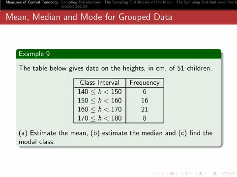
Example 9
The table below gives data on the heights, in cm, of 51 children.
Class Interval Frequency
140 ≤ h < 150 6150 ≤ h < 160 16160 ≤ h < 170 21170 ≤ h < 180 8
(a) Estimate the mean, (b) estimate the median and (c) find themodal class.
Measures of Central Tendency Sampling Distributions The Sampling Distribution of the Mean The Sampling Distribution of the M
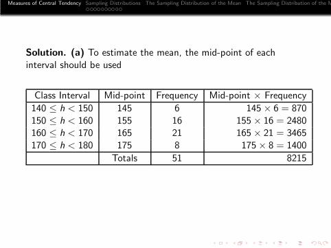
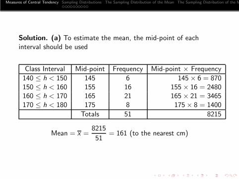
Solution. (a) To estimate the mean, the mid-point of eachinterval should be used
Class Interval Mid-point Frequency Mid-point × Frequency
140 ≤ h < 150 145 6 145 × 6 = 870150 ≤ h < 160 155 16 155 × 16 = 2480160 ≤ h < 170 165 21 165 × 21 = 3465170 ≤ h < 180 175 8 175× 8 = 1400
Totals 51 8215
Measures of Central Tendency Sampling Distributions The Sampling Distribution of the Mean The Sampling Distribution of the M
Solution. (a) To estimate the mean, the mid-point of eachinterval should be used
Class Interval Mid-point Frequency Mid-point × Frequency
140 ≤ h < 150 145 6 145 × 6 = 870150 ≤ h < 160 155 16 155 × 16 = 2480160 ≤ h < 170 165 21 165 × 21 = 3465170 ≤ h < 180 175 8 175× 8 = 1400
Totals 51 8215
Mean = x =8215
51= 161 (to the nearest cm)
Measures of Central Tendency Sampling Distributions The Sampling Distribution of the Mean The Sampling Distribution of the M
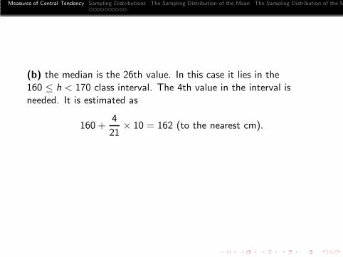
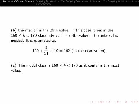
(b) the median is the 26th value. In this case it lies in the160 ≤ h < 170 class interval. The 4th value in the interval isneeded. It is estimated as
160 +4
21× 10 = 162 (to the nearest cm).
Measures of Central Tendency Sampling Distributions The Sampling Distribution of the Mean The Sampling Distribution of the M
(b) the median is the 26th value. In this case it lies in the160 ≤ h < 170 class interval. The 4th value in the interval isneeded. It is estimated as
160 +4
21× 10 = 162 (to the nearest cm).
(c) The modal class is 160 ≤ h < 170 as it contains the mostvalues.
Measures of Central Tendency Sampling Distributions The Sampling Distribution of the Mean The Sampling Distribution of the M
Note.
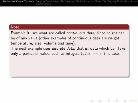
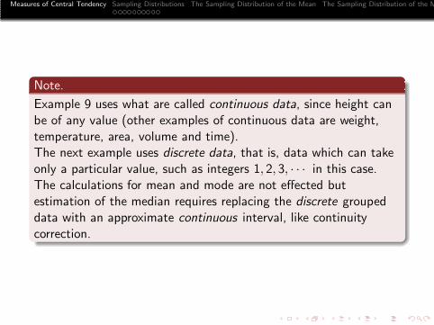
Example 9 uses what are called continuous data, since height canbe of any value (other examples of continuous data are weight,temperature, area, volume and time).
Measures of Central Tendency Sampling Distributions The Sampling Distribution of the Mean The Sampling Distribution of the M
Note.
Example 9 uses what are called continuous data, since height canbe of any value (other examples of continuous data are weight,temperature, area, volume and time).The next example uses discrete data, that is, data which can takeonly a particular value, such as integers 1, 2, 3, · · · in this case.
Measures of Central Tendency Sampling Distributions The Sampling Distribution of the Mean The Sampling Distribution of the M
Note.
Example 9 uses what are called continuous data, since height canbe of any value (other examples of continuous data are weight,temperature, area, volume and time).The next example uses discrete data, that is, data which can takeonly a particular value, such as integers 1, 2, 3, · · · in this case.The calculations for mean and mode are not effected butestimation of the median requires replacing the discrete groupeddata with an approximate continuous interval, like continuitycorrection.
Measures of Central Tendency Sampling Distributions The Sampling Distribution of the Mean The Sampling Distribution of the M
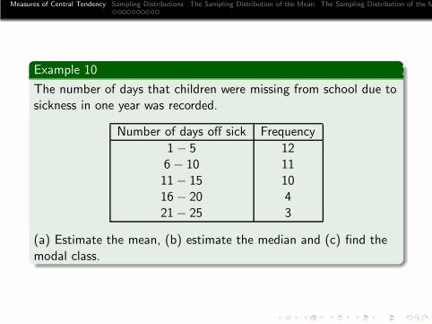
Example 10
The number of days that children were missing from school due tosickness in one year was recorded.
Number of days off sick Frequency
1− 5 126− 10 1111− 15 1016− 20 421− 25 3
(a) Estimate the mean, (b) estimate the median and (c) find themodal class.
Measures of Central Tendency Sampling Distributions The Sampling Distribution of the Mean The Sampling Distribution of the M
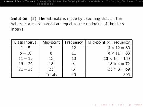
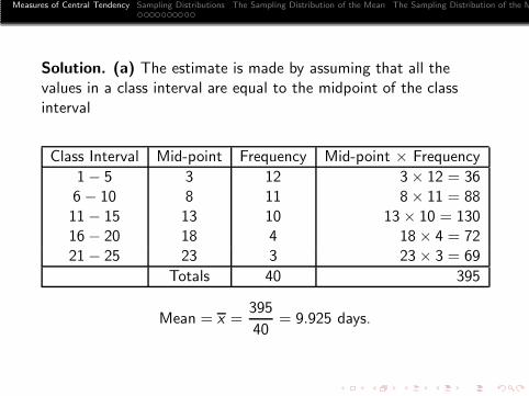
Solution. (a) The estimate is made by assuming that all thevalues in a class interval are equal to the midpoint of the classinterval
Class Interval Mid-point Frequency Mid-point × Frequency
1− 5 3 12 3× 12 = 366− 10 8 11 8× 11 = 8811− 15 13 10 13× 10 = 13016− 20 18 4 18× 4 = 7221− 25 23 3 23× 3 = 69
Totals 40 395
Measures of Central Tendency Sampling Distributions The Sampling Distribution of the Mean The Sampling Distribution of the M
Solution. (a) The estimate is made by assuming that all thevalues in a class interval are equal to the midpoint of the classinterval
Class Interval Mid-point Frequency Mid-point × Frequency
1− 5 3 12 3× 12 = 366− 10 8 11 8× 11 = 8811− 15 13 10 13× 10 = 13016− 20 18 4 18× 4 = 7221− 25 23 3 23× 3 = 69
Totals 40 395
Mean = x =395
40= 9.925 days.
Measures of Central Tendency Sampling Distributions The Sampling Distribution of the Mean The Sampling Distribution of the M
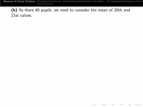
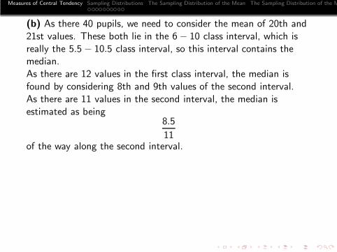
(b) As there 40 pupils, we need to consider the mean of 20th and21st values.
Measures of Central Tendency Sampling Distributions The Sampling Distribution of the Mean The Sampling Distribution of the M
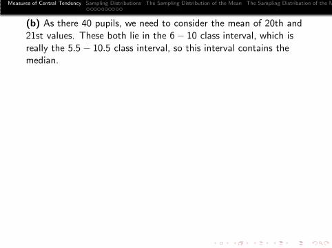
(b) As there 40 pupils, we need to consider the mean of 20th and21st values. These both lie in the 6− 10 class interval, which isreally the 5.5− 10.5 class interval, so this interval contains themedian.
Measures of Central Tendency Sampling Distributions The Sampling Distribution of the Mean The Sampling Distribution of the M
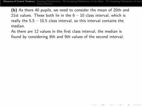
(b) As there 40 pupils, we need to consider the mean of 20th and21st values. These both lie in the 6− 10 class interval, which isreally the 5.5− 10.5 class interval, so this interval contains themedian.As there are 12 values in the first class interval, the median isfound by considering 8th and 9th values of the second interval.
Measures of Central Tendency Sampling Distributions The Sampling Distribution of the Mean The Sampling Distribution of the M
(b) As there 40 pupils, we need to consider the mean of 20th and21st values. These both lie in the 6− 10 class interval, which isreally the 5.5− 10.5 class interval, so this interval contains themedian.As there are 12 values in the first class interval, the median isfound by considering 8th and 9th values of the second interval.As there are 11 values in the second interval, the median isestimated as being
8.5
11of the way along the second interval.
Measures of Central Tendency Sampling Distributions The Sampling Distribution of the Mean The Sampling Distribution of the M
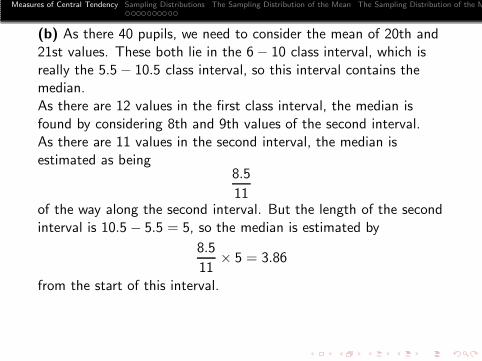
(b) As there 40 pupils, we need to consider the mean of 20th and21st values. These both lie in the 6− 10 class interval, which isreally the 5.5− 10.5 class interval, so this interval contains themedian.As there are 12 values in the first class interval, the median isfound by considering 8th and 9th values of the second interval.As there are 11 values in the second interval, the median isestimated as being
8.5
11of the way along the second interval. But the length of the secondinterval is 10.5 − 5.5 = 5, so the median is estimated by
8.5
11× 5 = 3.86
from the start of this interval.

Measures of Central Tendency Sampling Distributions The Sampling Distribution of the Mean The Sampling Distribution of the M
(b) As there 40 pupils, we need to consider the mean of 20th and21st values. These both lie in the 6− 10 class interval, which isreally the 5.5− 10.5 class interval, so this interval contains themedian.As there are 12 values in the first class interval, the median isfound by considering 8th and 9th values of the second interval.As there are 11 values in the second interval, the median isestimated as being
8.5
11of the way along the second interval. But the length of the secondinterval is 10.5 − 5.5 = 5, so the median is estimated by
8.5
11× 5 = 3.86
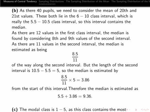
from the start of this interval.Therefore the median is estimated as
5.5 + 3.86 = 9.36.
Measures of Central Tendency Sampling Distributions The Sampling Distribution of the Mean The Sampling Distribution of the M
(b) As there 40 pupils, we need to consider the mean of 20th and21st values. These both lie in the 6− 10 class interval, which isreally the 5.5− 10.5 class interval, so this interval contains themedian.As there are 12 values in the first class interval, the median isfound by considering 8th and 9th values of the second interval.As there are 11 values in the second interval, the median isestimated as being
8.5
11of the way along the second interval. But the length of the secondinterval is 10.5 − 5.5 = 5, so the median is estimated by
8.5
11× 5 = 3.86
from the start of this interval.Therefore the median is estimated as
5.5 + 3.86 = 9.36.
(c) The modal class is 1− 5, as this class contains the most
Measures of Central Tendency Sampling Distributions The Sampling Distribution of the Mean The Sampling Distribution of the M
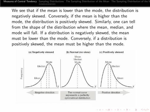
We see that if the mean is lower than the mode, the distribution isnegatively skewed. Conversely, if the mean is higher than themode, the distribution is positively skewed. Similarly, one can tellfrom the shape of the distribution where the mean, median, andmode will fall. If a distribution is negatively skewed, the meanmust be lower than the mode. Conversely, if a distribution ispositively skewed, the mean must be higher than the mode.
Measures of Central Tendency Sampling Distributions The Sampling Distribution of the Mean The Sampling Distribution of the M
Outline
1 Measures of Central Tendency
2 Sampling DistributionsPopulation and Sample. Statistical InferenceSampling With and Without ReplacementRandom Samples
3 The Sampling Distribution of the Mean
4 The Sampling Distribution of the Mean: Finite Population
Measures of Central Tendency Sampling Distributions The Sampling Distribution of the Mean The Sampling Distribution of the M
Population and Sample. Statistical Inference
Often in practice we are interested in drawing valid conclusionsabout a large group of individuals or objects.
Measures of Central Tendency Sampling Distributions The Sampling Distribution of the Mean The Sampling Distribution of the M
Population and Sample. Statistical Inference
Often in practice we are interested in drawing valid conclusionsabout a large group of individuals or objects. Instead of examiningthe entire group,
Measures of Central Tendency Sampling Distributions The Sampling Distribution of the Mean The Sampling Distribution of the M
Population and Sample. Statistical Inference
Often in practice we are interested in drawing valid conclusionsabout a large group of individuals or objects. Instead of examiningthe entire group, called the population,
Measures of Central Tendency Sampling Distributions The Sampling Distribution of the Mean The Sampling Distribution of the M
Population and Sample. Statistical Inference
Often in practice we are interested in drawing valid conclusionsabout a large group of individuals or objects. Instead of examiningthe entire group, called the population, which may be difficult orimpossible to do,
Measures of Central Tendency Sampling Distributions The Sampling Distribution of the Mean The Sampling Distribution of the M
Population and Sample. Statistical Inference
Often in practice we are interested in drawing valid conclusionsabout a large group of individuals or objects. Instead of examiningthe entire group, called the population, which may be difficult orimpossible to do, we may examine only a small part of thispopulation, which is called a sample.
Measures of Central Tendency Sampling Distributions The Sampling Distribution of the Mean The Sampling Distribution of the M
Population and Sample. Statistical Inference
Often in practice we are interested in drawing valid conclusionsabout a large group of individuals or objects. Instead of examiningthe entire group, called the population, which may be difficult orimpossible to do, we may examine only a small part of thispopulation, which is called a sample. We do this with the aim ofinferring certain facts about the population from results found inthe sample, a process known as statistical inference.
Measures of Central Tendency Sampling Distributions The Sampling Distribution of the Mean The Sampling Distribution of the M
Population and Sample. Statistical Inference
Often in practice we are interested in drawing valid conclusionsabout a large group of individuals or objects. Instead of examiningthe entire group, called the population, which may be difficult orimpossible to do, we may examine only a small part of thispopulation, which is called a sample. We do this with the aim ofinferring certain facts about the population from results found inthe sample, a process known as statistical inference. The processof obtaining samples is called sampling.
Measures of Central Tendency Sampling Distributions The Sampling Distribution of the Mean The Sampling Distribution of the M
Example 11
We may wish to draw conclusions about the heights (or weights)of 12,000 adult students (the population) by examining only 100students (a sample) selected from this population.
Example 12
We may wish to draw conclusions about the percentage ofdefective bolts produced in a factory during a given 6-day week byexamining 20 bolts each day produced at various times during theday. In this case all bolts produced during the week comprise thepopulation, while the 120 selected bolts constitute a sample.
Measures of Central Tendency Sampling Distributions The Sampling Distribution of the Mean The Sampling Distribution of the M
Example 13
We may wish to draw conclusions about the fairness of a particularcoin by tossing it repeatedly. The population consists of allpossible tosses of the coin. A sample could be obtained byexamining, say, the first 60 tosses of the coin and noting thepercentages of heads and tails.
Example 14
We may wish to draw conclusions about the colors of 200 marbles(the population) in an urn by selecting a sample of 20 marblesfrom the urn, where each marble selected is returned after its coloris observed.
Measures of Central Tendency Sampling Distributions The Sampling Distribution of the Mean The Sampling Distribution of the M
Several things should be noted. First, the word population doesnot necessarily have the same meaning as in everyday language,such as “the population of Abuja is 778.567.”
Measures of Central Tendency Sampling Distributions The Sampling Distribution of the Mean The Sampling Distribution of the M
Several things should be noted. First, the word population doesnot necessarily have the same meaning as in everyday language,such as “the population of Abuja is 778.567.” Second, the wordpopulation is often used to denote the observations ormeasurements rather than the individuals or objects.
Measures of Central Tendency Sampling Distributions The Sampling Distribution of the Mean The Sampling Distribution of the M
Several things should be noted. First, the word population doesnot necessarily have the same meaning as in everyday language,such as “the population of Abuja is 778.567.” Second, the wordpopulation is often used to denote the observations ormeasurements rather than the individuals or objects. In Example11 we can speak of the population of 12.000 heights (or weights)while in Example 14 we can speak of the population of all 200colors in the urn (some of which may be the same).
Measures of Central Tendency Sampling Distributions The Sampling Distribution of the Mean The Sampling Distribution of the M
Several things should be noted. First, the word population doesnot necessarily have the same meaning as in everyday language,such as “the population of Abuja is 778.567.” Second, the wordpopulation is often used to denote the observations ormeasurements rather than the individuals or objects. In Example11 we can speak of the population of 12.000 heights (or weights)while in Example 14 we can speak of the population of all 200colors in the urn (some of which may be the same). Third, thepopulation can be finite or infinite, the number being called thepopulation size, usually denoted by N.
Measures of Central Tendency Sampling Distributions The Sampling Distribution of the Mean The Sampling Distribution of the M
Several things should be noted. First, the word population doesnot necessarily have the same meaning as in everyday language,such as “the population of Abuja is 778.567.” Second, the wordpopulation is often used to denote the observations ormeasurements rather than the individuals or objects. In Example11 we can speak of the population of 12.000 heights (or weights)while in Example 14 we can speak of the population of all 200colors in the urn (some of which may be the same). Third, thepopulation can be finite or infinite, the number being called thepopulation size, usually denoted by N. Similarly the number in thesample is called the sample size, denoted by n, and is generallyfinite.
Measures of Central Tendency Sampling Distributions The Sampling Distribution of the Mean The Sampling Distribution of the M
Several things should be noted. First, the word population doesnot necessarily have the same meaning as in everyday language,such as “the population of Abuja is 778.567.” Second, the wordpopulation is often used to denote the observations ormeasurements rather than the individuals or objects. In Example11 we can speak of the population of 12.000 heights (or weights)while in Example 14 we can speak of the population of all 200colors in the urn (some of which may be the same). Third, thepopulation can be finite or infinite, the number being called thepopulation size, usually denoted by N. Similarly the number in thesample is called the sample size, denoted by n, and is generallyfinite. In Example 11, N = 12.000, n = 100, while in Example 13,N is infinite, n = 60.
Definition 15 (Population)
A set of numbers from which a sample is drawn is referred to as apopulation. The distribution of the numbers constituting apopulation is called population distribution.

Measures of Central Tendency Sampling Distributions The Sampling Distribution of the Mean The Sampling Distribution of the M
Sampling With and Without Replacement
If we draw an object from an urn, we have the choice of replacingor not replacing the object into the urn before we draw again.

Measures of Central Tendency Sampling Distributions The Sampling Distribution of the Mean The Sampling Distribution of the M
Sampling With and Without Replacement
If we draw an object from an urn, we have the choice of replacingor not replacing the object into the urn before we draw again. Inthe first case a particular object can come up again and again,whereas in the second it can come up only once.
Measures of Central Tendency Sampling Distributions The Sampling Distribution of the Mean The Sampling Distribution of the M
Sampling With and Without Replacement
If we draw an object from an urn, we have the choice of replacingor not replacing the object into the urn before we draw again. Inthe first case a particular object can come up again and again,whereas in the second it can come up only once. Sampling whereeach member of a population may be chosen more than once iscalled sampling with replacement, while sampling where eachmember cannot be chosen more than once is called samplingwithout replacement.
Measures of Central Tendency Sampling Distributions The Sampling Distribution of the Mean The Sampling Distribution of the M
Sampling With and Without Replacement
If we draw an object from an urn, we have the choice of replacingor not replacing the object into the urn before we draw again. Inthe first case a particular object can come up again and again,whereas in the second it can come up only once. Sampling whereeach member of a population may be chosen more than once iscalled sampling with replacement, while sampling where eachmember cannot be chosen more than once is called samplingwithout replacement.A finite population that is sampled with replacement cantheoretically be considered infinite since samples of any size can bedrawn without exhausting the population.
Measures of Central Tendency Sampling Distributions The Sampling Distribution of the Mean The Sampling Distribution of the M
Sampling With and Without Replacement
If we draw an object from an urn, we have the choice of replacingor not replacing the object into the urn before we draw again. Inthe first case a particular object can come up again and again,whereas in the second it can come up only once. Sampling whereeach member of a population may be chosen more than once iscalled sampling with replacement, while sampling where eachmember cannot be chosen more than once is called samplingwithout replacement.A finite population that is sampled with replacement cantheoretically be considered infinite since samples of any size can bedrawn without exhausting the population. For most practicalpurposes, sampling from a finite population that is very large canbe considered as sampling from an infinite population.
Measures of Central Tendency Sampling Distributions The Sampling Distribution of the Mean The Sampling Distribution of the M
Random Samples
Clearly, the reliability of conclusions drawn concerning a populationdepends on whether the sample is properly chosen so as torepresent the population sufficiently well, and one of the importantproblems of statistical inference is just how to choose a sample.
Measures of Central Tendency Sampling Distributions The Sampling Distribution of the Mean The Sampling Distribution of the M
Random Samples
Clearly, the reliability of conclusions drawn concerning a populationdepends on whether the sample is properly chosen so as torepresent the population sufficiently well, and one of the importantproblems of statistical inference is just how to choose a sample.One way to do this for finite populations is to make sure that eachmember of the population has the same chance of being in thesample, which is then often called a random sample.
Definition 16 (Random Sample)
If X1,X2, · · · ,Xn are independent and identically distributedrandom variables, we say that they constitute a random samplefrom the infinite population given by their common distribution.
Measures of Central Tendency Sampling Distributions The Sampling Distribution of the Mean The Sampling Distribution of the M
If f (x1, x2, · · · , xn) is the value of the joint distribution of such setof random variables at (x1, x2, · · · , xn), by virtue of independencewe can write
f (x1, x2, · · · , xn) =n∏
i=1
f (xi )
where f (xi ) is the value of the population distribution at xi .
Measures of Central Tendency Sampling Distributions The Sampling Distribution of the Mean The Sampling Distribution of the M
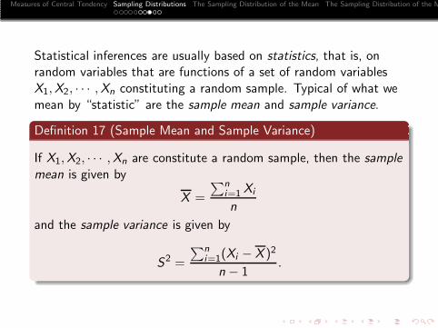
Statistical inferences are usually based on statistics, that is, onrandom variables that are functions of a set of random variablesX1,X2, · · · ,Xn constituting a random sample.
Measures of Central Tendency Sampling Distributions The Sampling Distribution of the Mean The Sampling Distribution of the M
Statistical inferences are usually based on statistics, that is, onrandom variables that are functions of a set of random variablesX1,X2, · · · ,Xn constituting a random sample. Typical of what wemean by “statistic” are the sample mean and sample variance.
Definition 17 (Sample Mean and Sample Variance)
If X1,X2, · · · ,Xn are constitute a random sample, then the samplemean is given by
X =
∑ni=1 Xi
n
and the sample variance is given by
S2 =
∑ni=1(Xi − X )2
n − 1.
Measures of Central Tendency Sampling Distributions The Sampling Distribution of the Mean The Sampling Distribution of the M
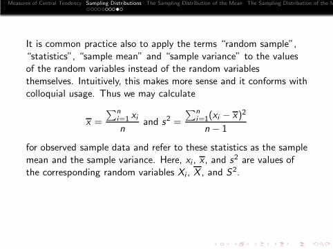
It is common practice also to apply the terms “random sample”,“statistics”, “sample mean” and “sample variance” to the valuesof the random variables instead of the random variablesthemselves.
Measures of Central Tendency Sampling Distributions The Sampling Distribution of the Mean The Sampling Distribution of the M
It is common practice also to apply the terms “random sample”,“statistics”, “sample mean” and “sample variance” to the valuesof the random variables instead of the random variablesthemselves. Intuitively, this makes more sense and it conforms withcolloquial usage.
Measures of Central Tendency Sampling Distributions The Sampling Distribution of the Mean The Sampling Distribution of the M
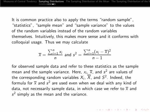
It is common practice also to apply the terms “random sample”,“statistics”, “sample mean” and “sample variance” to the valuesof the random variables instead of the random variablesthemselves. Intuitively, this makes more sense and it conforms withcolloquial usage. Thus we may calculate
x =
∑ni=1 xin
and s2 =
∑ni=1(xi − x)2
n − 1
for observed sample data and refer to these statistics as the samplemean and the sample variance.
Measures of Central Tendency Sampling Distributions The Sampling Distribution of the Mean The Sampling Distribution of the M
It is common practice also to apply the terms “random sample”,“statistics”, “sample mean” and “sample variance” to the valuesof the random variables instead of the random variablesthemselves. Intuitively, this makes more sense and it conforms withcolloquial usage. Thus we may calculate
x =
∑ni=1 xin
and s2 =
∑ni=1(xi − x)2
n − 1
for observed sample data and refer to these statistics as the samplemean and the sample variance. Here, xi , x , and s2 are values ofthe corresponding random variables Xi , X , and S2.
Measures of Central Tendency Sampling Distributions The Sampling Distribution of the Mean The Sampling Distribution of the M
It is common practice also to apply the terms “random sample”,“statistics”, “sample mean” and “sample variance” to the valuesof the random variables instead of the random variablesthemselves. Intuitively, this makes more sense and it conforms withcolloquial usage. Thus we may calculate
x =
∑ni=1 xin
and s2 =
∑ni=1(xi − x)2
n − 1
for observed sample data and refer to these statistics as the samplemean and the sample variance. Here, xi , x , and s2 are values ofthe corresponding random variables Xi , X , and S2. Indeed, theformula for x and s2 are used even when we deal with any kind ofdata, not necessarily sample data, in which case we refer to x ands2 simply as the mean and the variance.
Measures of Central Tendency Sampling Distributions The Sampling Distribution of the Mean The Sampling Distribution of the M
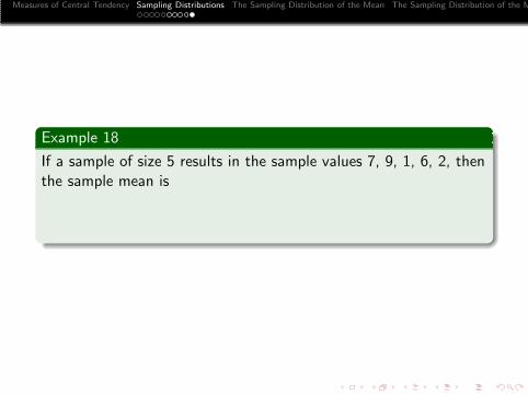
Example 18
If a sample of size 5 results in the sample values 7, 9, 1, 6, 2, thenthe sample mean is
Measures of Central Tendency Sampling Distributions The Sampling Distribution of the Mean The Sampling Distribution of the M
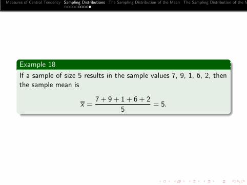
Example 18
If a sample of size 5 results in the sample values 7, 9, 1, 6, 2, thenthe sample mean is
x =7 + 9 + 1 + 6 + 2
5= 5.
Measures of Central Tendency Sampling Distributions The Sampling Distribution of the Mean The Sampling Distribution of the M
Outline
1 Measures of Central Tendency
2 Sampling DistributionsPopulation and Sample. Statistical InferenceSampling With and Without ReplacementRandom Samples
3 The Sampling Distribution of the Mean
4 The Sampling Distribution of the Mean: Finite Population
Measures of Central Tendency Sampling Distributions The Sampling Distribution of the Mean The Sampling Distribution of the M
The Sampling Distribution of the Mean
Let f (x) be the probability distribution of some given populationfrom which we draw a sample of size n.
Measures of Central Tendency Sampling Distributions The Sampling Distribution of the Mean The Sampling Distribution of the M
The Sampling Distribution of the Mean
Let f (x) be the probability distribution of some given populationfrom which we draw a sample of size n. Then it is natural to lookfor the probability distribution of the sample statistic X , which iscalled the sampling distribution for the sample mean, or thesampling distribution of means.
Measures of Central Tendency Sampling Distributions The Sampling Distribution of the Mean The Sampling Distribution of the M
The Sampling Distribution of the Mean
Let f (x) be the probability distribution of some given populationfrom which we draw a sample of size n. Then it is natural to lookfor the probability distribution of the sample statistic X , which iscalled the sampling distribution for the sample mean, or thesampling distribution of means. The following theorems areimportant in this connection.
Measures of Central Tendency Sampling Distributions The Sampling Distribution of the Mean The Sampling Distribution of the M
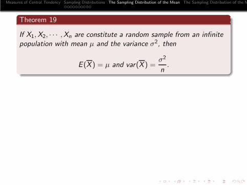
Theorem 19
If X1,X2, · · · ,Xn are constitute a random sample from an infinitepopulation with mean μ and the variance σ2, then
E (X ) = μ and var(X ) =σ2
n.
Measures of Central Tendency Sampling Distributions The Sampling Distribution of the Mean The Sampling Distribution of the M
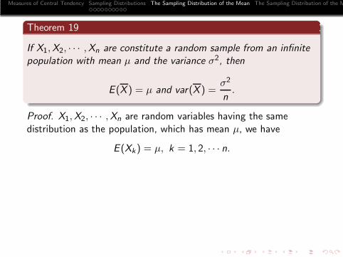
Theorem 19
If X1,X2, · · · ,Xn are constitute a random sample from an infinitepopulation with mean μ and the variance σ2, then
E (X ) = μ and var(X ) =σ2
n.
Proof. X1,X2, · · · ,Xn are random variables having the samedistribution as the population, which has mean μ, we have
E (Xk) = μ, k = 1, 2, · · · n.
Measures of Central Tendency Sampling Distributions The Sampling Distribution of the Mean The Sampling Distribution of the M
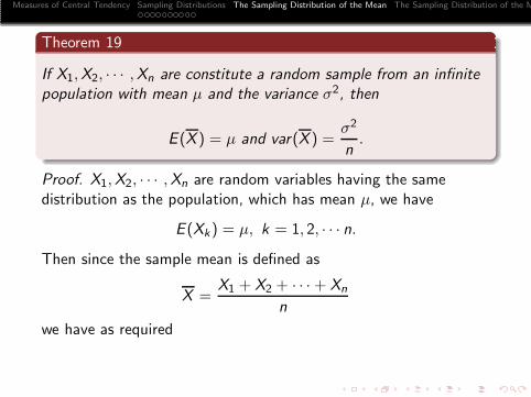
Theorem 19
If X1,X2, · · · ,Xn are constitute a random sample from an infinitepopulation with mean μ and the variance σ2, then
E (X ) = μ and var(X ) =σ2
n.
Proof. X1,X2, · · · ,Xn are random variables having the samedistribution as the population, which has mean μ, we have
E (Xk) = μ, k = 1, 2, · · · n.Then since the sample mean is defined as
X =X1 + X2 + · · ·+ Xn
n
we have as required
Measures of Central Tendency Sampling Distributions The Sampling Distribution of the Mean The Sampling Distribution of the M
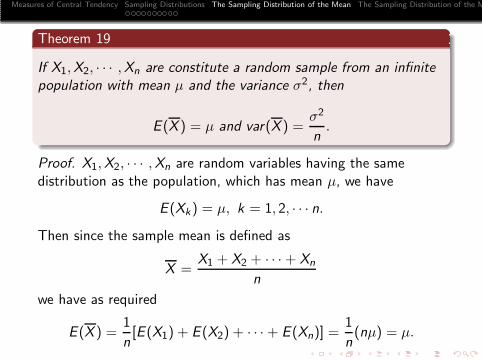
Theorem 19
If X1,X2, · · · ,Xn are constitute a random sample from an infinitepopulation with mean μ and the variance σ2, then
E (X ) = μ and var(X ) =σ2
n.
Proof. X1,X2, · · · ,Xn are random variables having the samedistribution as the population, which has mean μ, we have
E (Xk) = μ, k = 1, 2, · · · n.Then since the sample mean is defined as
X =X1 + X2 + · · ·+ Xn
n
we have as required
E (X ) =1
n[E (X1) + E (X2) + · · ·+ E (Xn)] =
1
n(nμ) = μ.
Measures of Central Tendency Sampling Distributions The Sampling Distribution of the Mean The Sampling Distribution of the M
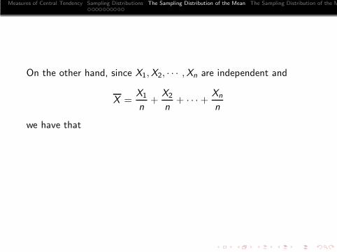
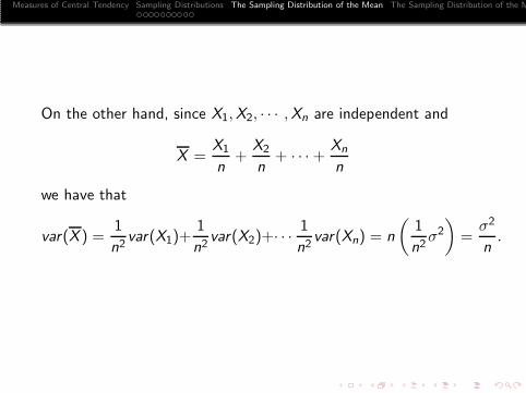
On the other hand, since X1,X2, · · · ,Xn are independent and
X =X1
n+
X2
n+ · · ·+ Xn
n
we have that
Measures of Central Tendency Sampling Distributions The Sampling Distribution of the Mean The Sampling Distribution of the M
On the other hand, since X1,X2, · · · ,Xn are independent and
X =X1
n+
X2
n+ · · ·+ Xn
n
we have that
var(X ) =1
n2var(X1)+
1
n2var(X2)+· · · 1
n2var(Xn) = n
(1
n2σ2
)=
σ2
n.
Measures of Central Tendency Sampling Distributions The Sampling Distribution of the Mean The Sampling Distribution of the M
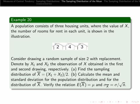
Example 20
A population consists of three housing units, where the value of X ,the number of rooms for rent in each unit, is shown in theillustration.
� � �
Consider drawing a random sample of size 2 with replacement.Denote by X1 and X2 the observation of X obtained in the firstand second drawing, respectively. (a) Find the samplingdistribution of X = (X1 + X2)/2. (b) Calculate the mean andstandard deviation for the population distribution and for thedistribution of X . Verify the relation E (X ) = μ and σX = σ/
√n.
Measures of Central Tendency Sampling Distributions The Sampling Distribution of the Mean The Sampling Distribution of the M
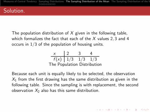
Solution.
The population distribution of X given in the following table,which formalizes the fact that each of the X values 2, 3 and 4occurs in 1/3 of the population of housing units.
x 2 3 4
f (x) 1/3 1/3 1/3The Population Distribution
Because each unit is equally likely to be selected, the observationX1 from the first drawing has the same distribution as given in thefollowing table. Since the sampling is with replacement, the secondobservation X2 also has this same distribution.
Measures of Central Tendency Sampling Distributions The Sampling Distribution of the Mean The Sampling Distribution of the M
Solution.
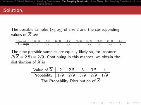
The possible samples (x1, x2) of size 2 and the correspondingvalues of X are
(x1, x2) (2, 2) (2, 3) (2, 4) (3, 2) (3, 3) (3, 4) (4, 2) (4, 3) (4, 4)
x =x1+x2
22 2.5 3 2.5 3 3.5 3 3.5 4
The nine possible samples are equally likely so, for instanceP(X = 2.5) = 2/9. Continuing in this manner, we obtain thedistribution of X is
Value of X 2 2.5 3 3.5 4
Probability 1/9 2/9 3/9 2/9 1/9
The Probability Distribution of X
Measures of Central Tendency Sampling Distributions The Sampling Distribution of the Mean The Sampling Distribution of the M
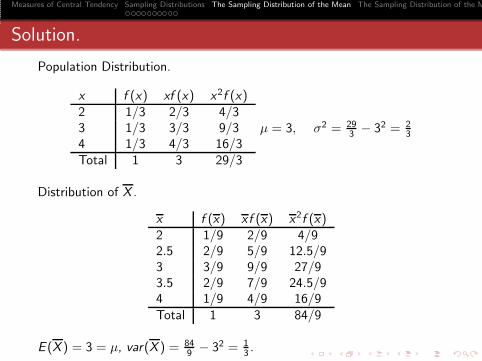
Solution.
Population Distribution.
x f (x) xf (x) x2f (x)2 1/3 2/3 4/33 1/3 3/3 9/34 1/3 4/3 16/3Total 1 3 29/3
μ = 3, σ2 = 293 − 32 = 2
3
Distribution of X .
x f (x) xf (x) x2f (x)2 1/9 2/9 4/92.5 2/9 5/9 12.5/93 3/9 9/9 27/93.5 2/9 7/9 24.5/94 1/9 4/9 16/9Total 1 3 84/9
E (X ) = 3 = μ, var(X ) = 849 − 32 = 1
3 .

Measures of Central Tendency Sampling Distributions The Sampling Distribution of the Mean The Sampling Distribution of the M
It is customary to write E (X ) as μX and var(X ) as σ2Xand σX as
the standard error of the mean.
Measures of Central Tendency Sampling Distributions The Sampling Distribution of the Mean The Sampling Distribution of the M
It is customary to write E (X ) as μX and var(X ) as σ2Xand σX as
the standard error of the mean. The formula for the standard errorof the mean, σX = σ/
√n, shows that the standard deviation of the
distribution of X decreases when n, the sample size, is increases.
Measures of Central Tendency Sampling Distributions The Sampling Distribution of the Mean The Sampling Distribution of the M
It is customary to write E (X ) as μX and var(X ) as σ2Xand σX as
the standard error of the mean. The formula for the standard errorof the mean, σX = σ/
√n, shows that the standard deviation of the
distribution of X decreases when n, the sample size, is increases.This means that when n becomes larger and we actually have moreinformation (the values of more random variables), we can expectvalues of X to be closer to μ, the quantity that they are intendedto estimate.
Measures of Central Tendency Sampling Distributions The Sampling Distribution of the Mean The Sampling Distribution of the M
It is customary to write E (X ) as μX and var(X ) as σ2Xand σX as
the standard error of the mean. The formula for the standard errorof the mean, σX = σ/
√n, shows that the standard deviation of the
distribution of X decreases when n, the sample size, is increases.This means that when n becomes larger and we actually have moreinformation (the values of more random variables), we can expectvalues of X to be closer to μ, the quantity that they are intendedto estimate. If we use Chebyshev’s theorem, we can express thisformally in the following way:
Theorem 21 (Law of Large Numbers)
For any positive constant c, the probability that X will take on avalue between μ− c and μ+ c is at least
1− σ2
nc2.
When n → ∞, this probability approaches 1.
Measures of Central Tendency Sampling Distributions The Sampling Distribution of the Mean The Sampling Distribution of the M
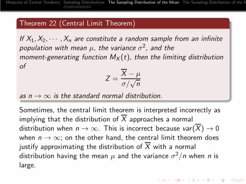
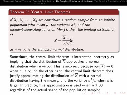
Theorem 22 (Central Limit Theorem)
If X1,X2, · · · ,Xn are constitute a random sample from an infinitepopulation with mean μ, the variance σ2, and themoment-generating function MX (t), then the limiting distributionof
Z =X − μ
σ/√n
as n → ∞ is the standard normal distribution.
Measures of Central Tendency Sampling Distributions The Sampling Distribution of the Mean The Sampling Distribution of the M
Theorem 22 (Central Limit Theorem)
If X1,X2, · · · ,Xn are constitute a random sample from an infinitepopulation with mean μ, the variance σ2, and themoment-generating function MX (t), then the limiting distributionof
Z =X − μ
σ/√n
as n → ∞ is the standard normal distribution.
Sometimes, the central limit theorem is interpreted incorrectly asimplying that the distribution of X approaches a normaldistribution when n → ∞.
Measures of Central Tendency Sampling Distributions The Sampling Distribution of the Mean The Sampling Distribution of the M
Theorem 22 (Central Limit Theorem)
If X1,X2, · · · ,Xn are constitute a random sample from an infinitepopulation with mean μ, the variance σ2, and themoment-generating function MX (t), then the limiting distributionof
Z =X − μ
σ/√n
as n → ∞ is the standard normal distribution.
Sometimes, the central limit theorem is interpreted incorrectly asimplying that the distribution of X approaches a normaldistribution when n → ∞. This is incorrect because var(X ) → 0when n → ∞; on the other hand, the central limit theorem doesjustify approximating the distribution of X with a normaldistribution having the mean μ and the variance σ2/n when n islarge.
Measures of Central Tendency Sampling Distributions The Sampling Distribution of the Mean The Sampling Distribution of the M
Theorem 22 (Central Limit Theorem)
If X1,X2, · · · ,Xn are constitute a random sample from an infinitepopulation with mean μ, the variance σ2, and themoment-generating function MX (t), then the limiting distributionof
Z =X − μ
σ/√n
as n → ∞ is the standard normal distribution.
Sometimes, the central limit theorem is interpreted incorrectly asimplying that the distribution of X approaches a normaldistribution when n → ∞. This is incorrect because var(X ) → 0when n → ∞; on the other hand, the central limit theorem doesjustify approximating the distribution of X with a normaldistribution having the mean μ and the variance σ2/n when n islarge. In practice, this approximation is used when n ≥ 30regardless of the actual shape of the population sampled.
Measures of Central Tendency Sampling Distributions The Sampling Distribution of the Mean The Sampling Distribution of the M
Example 23
A soft drink vending machine is set so that the amount of drinkdispensed is a random variable with mean of 200 milliliters and astandard deviation of 15 milliliters. What is the probability thatthe average (mean) amount dispensed in a random sample of size36 is at least 204 milliliters?
Measures of Central Tendency Sampling Distributions The Sampling Distribution of the Mean The Sampling Distribution of the M
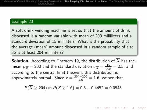
Example 23
A soft drink vending machine is set so that the amount of drinkdispensed is a random variable with mean of 200 milliliters and astandard deviation of 15 milliliters. What is the probability thatthe average (mean) amount dispensed in a random sample of size36 is at least 204 milliliters?
Solution. According to Theorem 19, the distribution of X has themean μX = 200 and the standard deviation σX = 15√
36= 2.5, and
according to the central limit theorem, this distribution isapproximately normal. Since z = 204−200
2.5 = 1.6, we see that
P(X ≥ 204) ≈ P(Z ≥ 1.6) = 0.5− 0.4452 = 0.0548.
Measures of Central Tendency Sampling Distributions The Sampling Distribution of the Mean The Sampling Distribution of the M
It is of interest to note that when the population we are samplingis normal, the distribution of X is a normal distribution regardlessof the size of n.
Measures of Central Tendency Sampling Distributions The Sampling Distribution of the Mean The Sampling Distribution of the M
It is of interest to note that when the population we are samplingis normal, the distribution of X is a normal distribution regardlessof the size of n.
Theorem 24
If X is the mean of a random sample of size n from a normalpopulation with mean μ and the variance σ2, its samplingdistribution is a normal distribution with mean μ and the varianceσ2/n.
Measures of Central Tendency Sampling Distributions The Sampling Distribution of the Mean The Sampling Distribution of the M
Outline
1 Measures of Central Tendency
2 Sampling DistributionsPopulation and Sample. Statistical InferenceSampling With and Without ReplacementRandom Samples
3 The Sampling Distribution of the Mean
4 The Sampling Distribution of the Mean: Finite Population
Measures of Central Tendency Sampling Distributions The Sampling Distribution of the Mean The Sampling Distribution of the M
The Sampling Distribution of the Mean: Finite Population
If an experiment consists of selecting one or more values from afinite set of numbers {c1, c2, · · · , cN}, this set is referred to as afinite population of size N.
Measures of Central Tendency Sampling Distributions The Sampling Distribution of the Mean The Sampling Distribution of the M
The Sampling Distribution of the Mean: Finite Population
If an experiment consists of selecting one or more values from afinite set of numbers {c1, c2, · · · , cN}, this set is referred to as afinite population of size N.In the definition that follows, it will beassumed that we are sampling without replacement from a finitepopulation of size N.
Definition 25 (Random Sample-Finite Population)
If X1 is the first value drawn from a finite population of size N, X2
is the second value drawn, . . . , Xn is the nth value drawn, and thejoint probability distribution of these n random variables is given by
f (x1, x2, · · · , xn) = 1
N(N − 1) · · · (N − n + 1)
for each ordered n-tuple of values of these random variables, thenX1,X2, · · · ,Xn are said to constitute a random sample from thegiven finite population.
Measures of Central Tendency Sampling Distributions The Sampling Distribution of the Mean The Sampling Distribution of the M
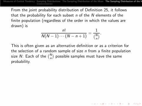
From the joint probability distribution of Definition 25, it followsthat the probability for each subset n of the N elements of thefinite population (regardless of the order in which the values aredrawn) is
n!
N(N − 1) · · · (N − n + 1)=
1(Nn
) .
Measures of Central Tendency Sampling Distributions The Sampling Distribution of the Mean The Sampling Distribution of the M
From the joint probability distribution of Definition 25, it followsthat the probability for each subset n of the N elements of thefinite population (regardless of the order in which the values aredrawn) is
n!
N(N − 1) · · · (N − n + 1)=
1(Nn
) .This is often given as an alternative definition or as a criterion forthe selection of a random sample of size n from a finite populationsize N:
Measures of Central Tendency Sampling Distributions The Sampling Distribution of the Mean The Sampling Distribution of the M
From the joint probability distribution of Definition 25, it followsthat the probability for each subset n of the N elements of thefinite population (regardless of the order in which the values aredrawn) is
n!
N(N − 1) · · · (N − n + 1)=
1(Nn
) .This is often given as an alternative definition or as a criterion forthe selection of a random sample of size n from a finite populationsize N: Each of the
(Nn
)possible samples must have the same
probability.
Measures of Central Tendency Sampling Distributions The Sampling Distribution of the Mean The Sampling Distribution of the M
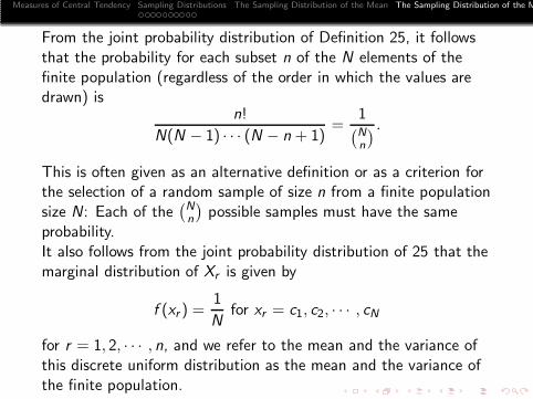
From the joint probability distribution of Definition 25, it followsthat the probability for each subset n of the N elements of thefinite population (regardless of the order in which the values aredrawn) is
n!
N(N − 1) · · · (N − n + 1)=
1(Nn
) .This is often given as an alternative definition or as a criterion forthe selection of a random sample of size n from a finite populationsize N: Each of the
(Nn
)possible samples must have the same
probability.It also follows from the joint probability distribution of 25 that themarginal distribution of Xr is given by
f (xr ) =1
Nfor xr = c1, c2, · · · , cN
for r = 1, 2, · · · , n, and we refer to the mean and the variance ofthis discrete uniform distribution as the mean and the variance ofthe finite population.
Measures of Central Tendency Sampling Distributions The Sampling Distribution of the Mean The Sampling Distribution of the M
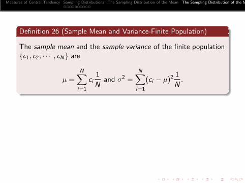
Definition 26 (Sample Mean and Variance-Finite Population)
The sample mean and the sample variance of the finite population{c1, c2, · · · , cN} are
μ =N∑i=1
ci1
Nand σ2 =
N∑i=1
(ci − μ)21
N.
Measures of Central Tendency Sampling Distributions The Sampling Distribution of the Mean The Sampling Distribution of the M
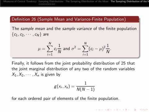
Definition 26 (Sample Mean and Variance-Finite Population)
The sample mean and the sample variance of the finite population{c1, c2, · · · , cN} are
μ =N∑i=1
ci1
Nand σ2 =
N∑i=1
(ci − μ)21
N.
Finally, it follows from the joint probability distribution of 25 thatthe joint marginal distribution of any two of the random variablesX1,X2, · · · ,Xn is given by
g(xr , xs) =1
N(N − 1)
for each ordered pair of elements of the finite population.
Measures of Central Tendency Sampling Distributions The Sampling Distribution of the Mean The Sampling Distribution of the M
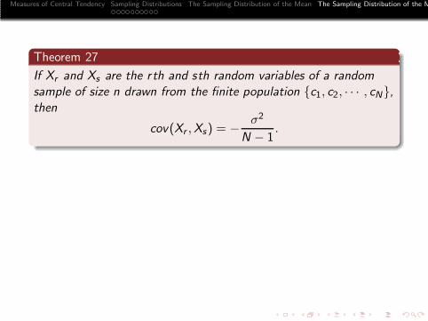
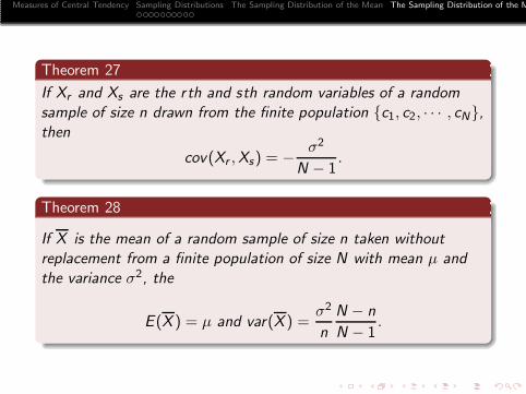
Theorem 27
If Xr and Xs are the rth and sth random variables of a randomsample of size n drawn from the finite population {c1, c2, · · · , cN},then
cov(Xr ,Xs) = − σ2
N − 1.
Measures of Central Tendency Sampling Distributions The Sampling Distribution of the Mean The Sampling Distribution of the M
Theorem 27
If Xr and Xs are the rth and sth random variables of a randomsample of size n drawn from the finite population {c1, c2, · · · , cN},then
cov(Xr ,Xs) = − σ2
N − 1.
Theorem 28
If X is the mean of a random sample of size n taken withoutreplacement from a finite population of size N with mean μ andthe variance σ2, the
E (X ) = μ and var(X ) =σ2
n
N − n
N − 1.
Measures of Central Tendency Sampling Distributions The Sampling Distribution of the Mean The Sampling Distribution of the M
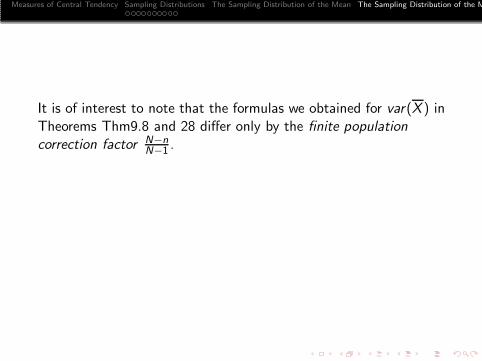
It is of interest to note that the formulas we obtained for var(X ) inTheorems Thm9.8 and 28 differ only by the finite populationcorrection factor N−n
N−1 .
Measures of Central Tendency Sampling Distributions The Sampling Distribution of the Mean The Sampling Distribution of the M
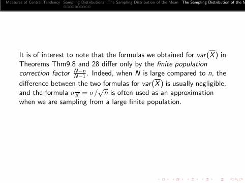
It is of interest to note that the formulas we obtained for var(X ) inTheorems Thm9.8 and 28 differ only by the finite populationcorrection factor N−n
N−1 . Indeed, when N is large compared to n, the
difference between the two formulas for var(X ) is usually negligible,and the formula σX = σ/
√n is often used as an approximation
when we are sampling from a large finite population.
Measures of Central Tendency Sampling Distributions The Sampling Distribution of the Mean The Sampling Distribution of the M
It is of interest to note that the formulas we obtained for var(X ) inTheorems Thm9.8 and 28 differ only by the finite populationcorrection factor N−n
N−1 . Indeed, when N is large compared to n, the
difference between the two formulas for var(X ) is usually negligible,and the formula σX = σ/
√n is often used as an approximation
when we are sampling from a large finite population. A generalrule of thumb is to use this approximation when the sampling doesnot constitute more than 5 percent of the population.
Measures of Central Tendency Sampling Distributions The Sampling Distribution of the Mean The Sampling Distribution of the M
Example 29
A population consists of the five numbers 2, 3, 6, 8, 11. Considerall possible samples of size two which can be drawn withreplacement from this population. Find (a) the mean of thepopulation, (b) the standard deviation of the population, (c) themean of the sampling distribution of means, (d) the standarddeviation of the sampling distribution of means, i.e., the standarderror of means.
Example 30
Solve Example 29 in case sampling is without replacement.
Measures of Central Tendency Sampling Distributions The Sampling Distribution of the Mean The Sampling Distribution of the M
Example 31
Assume that the heights of 3000 male students at a university arenormally distributed with mean 68.0 inches and standard deviation3.0 inches. If 80 samples consisting of 25 students each areobtained, what would be the mean and standard deviation of theresulting sample of means if sampling were done (a) withreplacement, (b) without replacement?
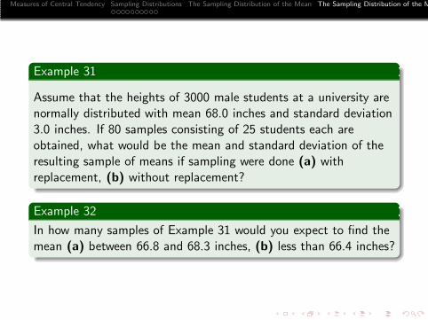
Example 32
In how many samples of Example 31 would you expect to find themean (a) between 66.8 and 68.3 inches, (b) less than 66.4 inches?
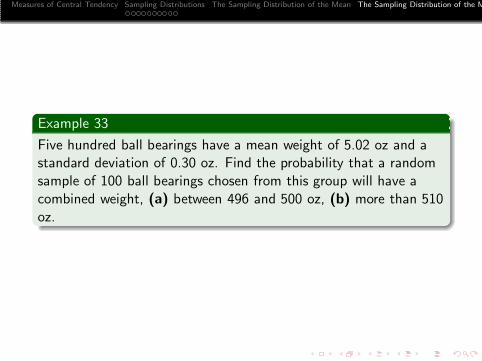
Measures of Central Tendency Sampling Distributions The Sampling Distribution of the Mean The Sampling Distribution of the M
Example 33
Five hundred ball bearings have a mean weight of 5.02 oz and astandard deviation of 0.30 oz. Find the probability that a randomsample of 100 ball bearings chosen from this group will have acombined weight, (a) between 496 and 500 oz, (b) more than 510oz.
Measures of Central Tendency Sampling Distributions The Sampling Distribution of the Mean The Sampling Distribution of the M
Thank You!!!