Lecture 7 Unconstrained nonlinear programming
43
Lecture 7 Unconstrained nonlinear programming Weinan E 1,2 and Tiejun Li 2 1 Department of Mathematics, Princeton University, [email protected] 2 School of Mathematical Sciences, Peking University, [email protected] No.1 Science Building, 1575
Transcript of Lecture 7 Unconstrained nonlinear programming

Lecture 7 Unconstrained nonlinear programming
Weinan E1,2 and Tiejun Li2
1Department of Mathematics,
Princeton University,
2School of Mathematical Sciences,
Peking University,
No.1 Science Building, 1575

Application examples Numerical methods
Outline
Application examples
Numerical methods

Application examples Numerical methods
Energy minimization: virtual drug design
I Virtual drug design is to find a best position of a ligand (a small protein
molecule) interacting with a large target protein molecule. It is equivalent
to an energy minimization problem.

Application examples Numerical methods
Energy minimization: protein folding
I Protein folding is to find the minimal energy state of a protein molecule
from its sequence structure. It is an outstanding open problem for global
optimization in the molecular mechanics.
Application examples Numerical methods
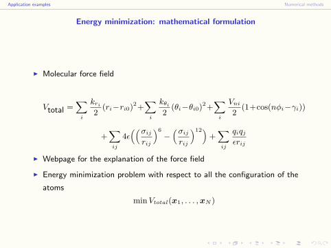
Energy minimization: mathematical formulation
I Molecular force field
Vtotal =∑
i
kri
2(ri−ri0)
2+∑
i
kθi
2(θi−θi0)
2+∑
i
Vni
2(1+cos(nφi−γi))
+∑ij
4ε((σij
rij
)6
−(σij
rij
)12)+
∑ij
qiqj
εrij
I Webpage for the explanation of the force field
I Energy minimization problem with respect to all the configuration of the
atoms
min Vtotal(x1, . . . , xN )
Application examples Numerical methods
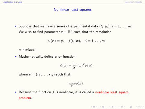
Nonlinear least squares
I Suppose that we have a series of experimental data (ti, yi), i = 1, . . . , m.
We wish to find parameter x ∈ Rn such that the remainder
ri(x) = yi − f(ti, x), i = 1, . . . , m
minimized.
I Mathematically, define error function
φ(x) =1
2r(x)T r(x)
where r = (r1, . . . , rm) such that
minx
φ(x).
I Because the function f is nonlinear, it is called a nonlinear least square
problem.

Application examples Numerical methods
Optimal control problem
I Classical optimal control problem:
min
∫ T
0
f(x, u)dt
such that the constraint
dx
dt= g(x, u), x(0) = x0, x(T ) = xT
is satisfied. Here u(t) is the control function, x(t) is the output.
I It is a nonlinear optimization in function space.
Application examples Numerical methods
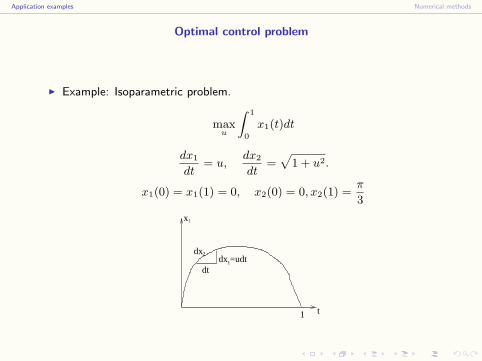
Optimal control problem
I Example: Isoparametric problem.
maxu
∫ 1
0
x1(t)dt
dx1
dt= u,
dx2
dt=
√1 + u2.
x1(0) = x1(1) = 0, x2(0) = 0, x2(1) =π
3
1 t
dtdx =udt1
dx2
x1

Application examples Numerical methods
Outline
Application examples
Numerical methods

Application examples Numerical methods
Iterations
I Iterative methods
Object: construct sequence {xk}∞k=1, such that xk converge to a fixed
vector x∗, and x∗ is the solution of the linear system.
I General iteration idea:
If we want to solve equations
g(x) = 0,
and the equation x = f(x) has the same solution as it, then construct
xk+1 = f(xk).
If xk → x∗, then x∗ = f(x∗), thus the root of g(x) is obtained.

Application examples Numerical methods
Convergence order
I Suppose an iterating sequence lim xn = x∗, and
|xn − x∗| ≤ εn
where εn is called error bound. If
limεn+1
εn= C,
when
1. 0 < C < 1, xn is called linear convergence;
q, q2, q3, · · · , qn, · · · , (q < 1)
2. C = 1, xn is called sublinear convergence;
1,1
2,1
3, · · · ,
1
n, · · ·
3. C = 0, xn is called superlinear convergence;
1,1
2!,
1
3!, · · · ,
1
n!, · · ·

Application examples Numerical methods
Convergence order
I If
limεn+1
εpn
= C, C > 0, p > 1
then xn is called p-th order convergence.
q, qp, qp2, · · · , qpn
, · · ·
I Numerical examples for different convergence orders
Application examples Numerical methods
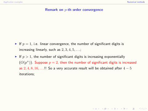
Remark on p-th order convergence
I If p = 1, i.e. linear convergence, the number of significant digits is
increasing linearly, such as 2, 3, 4, 5, . . .;
I If p > 1, the number of significant digits is increasing exponentially
(O(pn)). Suppose p = 2, then the number of significant digits is increased
as 2, 4, 8, 16, . . .!! So a very accurate result will be obtained after 4− 5
iterations;

Application examples Numerical methods
Golden section method
I Suppose there is a triplet (a, xk, c) and f(xk) < f(a), f(xk) < f(c), we
want to find xk+1 in (a, c) to perform a section. Suppose xk+1 is in
(a, xk).
a x ckx k+1
w
z1−w
I If f(xk+1) > f(xk), then the new search interval is (xk+1, c); If
f(xk+1) < f(xk), then the new search interval is (a, xk).

Application examples Numerical methods
Golden section method
I Define
w =xk − a
c− a, 1− w =
c− xk
c− a
and
z =xk − xk+1
c− a.
If we want to minimize the worst case possibility (for two cases), we must
make w = z + (1− w). (w > 12)
I Pay attention that w is also obtained from the previous stage of applying
same strategy. This scale similarity implies
z
w= 1− w
we have
w =
√5− 1
2≈ 0.618
This is called Golden section method.

Application examples Numerical methods
Golden section method
I Golden section method is a method to find the local minimum of a
function f .
I Golden section method is a linear convergence method. The contraction
coefficient is C = 0.618.
I Golden section method for Example
min ϕ(x) = 0.5− xe−x2
where a = 0, c = 2.
Application examples Numerical methods
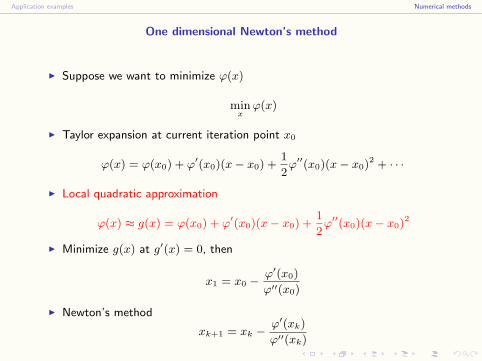
One dimensional Newton’s method
I Suppose we want to minimize ϕ(x)
minx
ϕ(x)
I Taylor expansion at current iteration point x0
ϕ(x) = ϕ(x0) + ϕ′(x0)(x− x0) +1
2ϕ′′(x0)(x− x0)
2 + · · ·
I Local quadratic approximation
ϕ(x) ≈ g(x) = ϕ(x0) + ϕ′(x0)(x− x0) +1
2ϕ′′(x0)(x− x0)
2
I Minimize g(x) at g′(x) = 0, then
x1 = x0 −ϕ′(x0)
ϕ′′(x0)
I Newton’s method
xk+1 = xk −ϕ′(xk)
ϕ′′(xk)

Application examples Numerical methods
One dimensional Newton’s method
I Graphical explanation
xkxk+1
Local parabolic approximation
I Example
min ϕ(x) = 0.5− xe−x2
where x0 = 0.5.
Application examples Numerical methods
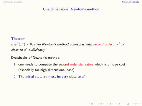
One dimensional Newton’s method
Theorem
If ϕ′′(x∗) 6= 0, then Newton’s method converges with second order if x0 is
close to x∗ sufficiently.
Drawbacks of Newton’s method:
1. one needs to compute the second order derivative which is a huge cost
(especially for high dimensional case).
2. The initial state x0 must be very close to x∗.

Application examples Numerical methods
High dimensional Newton’s method
I Suppose we want to minimize f(x), x ∈ Rn
minx
f(x)
I Taylor expansion at current iteration point x0
f(x) = f(x0) +∇f(x0) · (x− x0) +1
2(x− x0)
T∇2f(x0)(x− x0) + · · ·
I Local quadratic approximation
f(x) ≈ g(x) = f(x0) +∇f(x0) · (x−x0) +1
2(x−x0)
T Hf (x0)(x−x0)
where Hf is the Hessian matrix defined as (Hf )ij = ∂2f∂xi∂xj
.
I Minimize g(x) at ∇g(x) = 0, then
x1 = x0 −Hf (x0)−1 · ∇f(x0)
I Newton’s method
xk+1 = xk −Hf (xk)−1 · ∇f(xk)

Application examples Numerical methods
High dimensional Newton’s method
Example
min f(x1, x2) = 100(x2 − x21)
2 + (x1 − 1)2
Initial state x0 = (−1.2, 1).

Application examples Numerical methods
Steepest decent method
I Basic idea: Find a series of decent directions pk and corresponding
stepsize αk such that the iterations
xk+1 = xk + αkpk
and
f(xk+1) ≤ f(xk).
I The negative gradient direction −∇f is the “steepest” decent direction,
so choose
pk := −∇f(xk)
and choose αk such that
minα
f(xk + αpk)

Application examples Numerical methods
Inexact line search
I To find α such that
minα
f(xk + αpk)
is equivalent to perform a one dimensional minimization. But it is enough
to find an approximate α by the following inexact line search method.
I Inexact line search is to make the following type of the decent criterion
f(xk)− f(xk+1) ≥ ε0
is satisfied.

Application examples Numerical methods
Inexact line search
I An example of inexact line search strategy by half increment (or
decrement) method:
[a0, b0] = [0, +∞), α0 = 1; [a1, b1] = [0, 1], α1 =1
2
[a2, b2] = [0,1
2], α2 =
1
4; [a3, b3] = [
1
4,1
2], α3 =
3
8
· · · · · · · · · · · ·
a=0 b=1
3/81/4 1/2

Application examples Numerical methods
Steepest decent method
Steepest decent method for example
min f(x1, x2) = 100(x2 − x21)
2 + (x1 − 1)2
Initial state x0 = (−1.2, 1).

Application examples Numerical methods
Dumped Newton’s method
I If the initial value of Newton’s method is not near the minimum point, a
strategy is to apply dumped Newton’s method.
I Choose the decent direction as the Newton’s direction
pk := −H−1f (xk)∇f(xk)
and perform the inexact line search for
minα
f(xk + αpk)

Application examples Numerical methods
Conjugate gradient method
Recalling conjugate gradient method for quadratic function
ϕ(x) =1
2xT Ax− bT x
1. Initial step: x0, p0 = r0 = b−Ax0
2. Suppose we have xk, rk, pk, the CGM step
2.1 Search the optimal αk along pk;
αk =(rk)T pk
(pk)T Apk
2.2 Update xk and gradient direction rk;
xk+1 = xk + αkpk, rk+1 = b−Axk+1
2.3 According to the calculation before to form new search direction pk+1
βk = −(rk+1)T Apk
(pk)T Apk
, pk+1 = rk+1 + βkpk

Application examples Numerical methods
Conjugate gradient method
I Local quadratic approximation of general nonlinear optimization
f(x) ≈ f(x0) +∇f(x0) · (x− x0) +1
2(x− x0)
T Hf (x0)(x− x0)
where Hf (x0) is the Hessian of f at x0.
I Apply conjugate gradient method to the quadratic function above
successively.
I The computation of βk needs the formation of Hessian matrix Hf (x0)
which is a formidable task!
I Equivalent transformation in the quadratic case
βk = − (rk+1)T Apk
(pk)T Apk
=‖∇ϕ(xk+1)‖2
‖∇ϕ(xk)‖2
This formula does NOT need the computation of Hessian matrix.

Application examples Numerical methods
Conjugate gradient method for nonlinear optimization
Formally generalize CGM to nonlinear optimization
1. Given initial x0 and ε > 0;
2. Compute g0 = ∇f(x0) and p0 = −g0, k = 0;
3. Compute λk from
minλ
f(xk + λpk)
and
xk+1 = xk + λkpk, gk+1 = ∇f(xk+1)
4. If ‖gk+1‖ ≤ ε, the iteration is over. Otherwise compute
µk+1 =‖gk+1‖2
‖gk‖2
pk+1 = −gk+1 + µk+1pk
Set k = k + 1, iterate until convergence.

Application examples Numerical methods
Conjugate gradient method
In realistic computations, because there is only n conjugate gradient directions
for n dimensional problem, it often restarts from current point after n
iterations.
Application examples Numerical methods
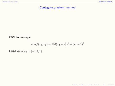
Conjugate gradient method
CGM for example
min f(x1, x2) = 100(x2 − x21)
2 + (x1 − 1)2
Initial state x0 = (−1.2, 1).

Application examples Numerical methods
Variable metric method
I A general form of iterations
xk+1 = xk − λkHk∇f(xk)
1. If Hk = I, it is steepest decent method;
2. If Hk = [∇2f(xk)]−1, it is dumped Newton’s method.
I In order to keep the fast convergence of Newton’s method, we hope to
approximate [∇2f(xk)]−1 as Hk with reduced computational efforts as
Hk+1 = Hk + Ck,
where Ck is a correction matrix which is easily computed.

Application examples Numerical methods
Variable metric method
I First consider quadratic function
f(x) = a + bT x +1
2xT Gx
we have
∇f(x) = b + Gx
I Define g(x) = ∇f(x), gk = g(xk), then
gk+1 − gk = G(xk+1 − xk).
Define
∆xk = xk+1 − xk, ∆gk = gk+1 − gk
we have
G∆xk = ∆gk.
Application examples Numerical methods
Variable metric method
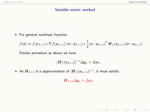
I For general nonlinear function
f(x) ≈ f(xk+1)+∇f(xk+1)·(x−xk+1)+1
2(x−xk+1)
T Hf (xk+1)(x−xk+1).
Similar procedure as above we have
[Hf (xk+1)]−1∆gk = ∆xk.
I As Hk+1 is a approximation of [Hf (xk+1)]−1, it must satisfy
Hk+1∆gk = ∆xk.
Application examples Numerical methods
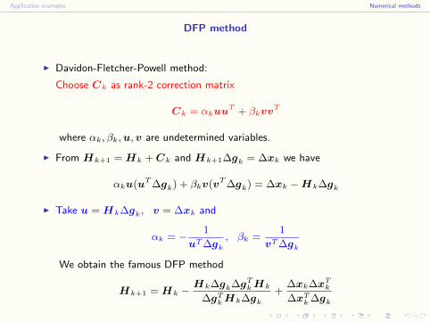
DFP method
I Davidon-Fletcher-Powell method:
Choose Ck as rank-2 correction matrix
Ck = αkuuT + βkvvT
where αk, βk, u, v are undetermined variables.
I From Hk+1 = Hk + Ck and Hk+1∆gk = ∆xk we have
αku(uT ∆gk) + βkv(vT ∆gk) = ∆xk −Hk∆gk
I Take u = Hk∆gk, v = ∆xk and
αk = − 1
uT ∆gk
, βk =1
vT ∆gk
We obtain the famous DFP method
Hk+1 = Hk −Hk∆gk∆gT
k Hk
∆gTk Hk∆gk
+∆xk∆xT
k
∆xTk ∆gk

Application examples Numerical methods
Remark on DFP method
I If f(x) is quadratic and H0 = I, then the result will converge in n steps
theoretically;
I If f(x) is strictly convex, the DFP method is convergent globally.
I If Hk is SPD and gk 6= 0, then Hk+1 is SPD also.

Application examples Numerical methods
DFP method
DFP method for example
min f(x1, x2) = 100(x2 − x21)
2 + (x1 − 1)2
Initial state x0 = (−1.2, 1).

Application examples Numerical methods
BFGS method
I The most popular variable metric method is BFGS
(Broyden-Fletcher-Goldfarb-Shanno) method shown as below
Hk+1 = Hk −Hk∆gk∆gT
k Hk
∆gTk Hk∆gk
+∆xk∆xT
k
∆xTk ∆gk
+ (∆gTk Hk∆gk)vkvT
k
where
vk =∆xk
∆xTk ∆gk
− Hk∆gk
∆gTk Hk∆gk
I BFGS is more stable than DFP method;
I BFGS is also a rank-2 correction method for Hk.

Application examples Numerical methods
Nonlinear least squares
I Mathematically, nonlinear least squares is to minimize
φ(x) =1
2r(x)T r(x)
I We have
∇φ(x) = JT (x)r(x), Hφ(x) = JT (x)J(x) +
m∑i=1
ri(x)Hri(x)
where J(x) is the Jacobian matrix of r(x).
I Direct Newton’s method for increment sk in nonlinear least squares
Hφ(xk)sk = −∇φ(xk)

Application examples Numerical methods
Gauss-Newton method
I If make the assumption that the residual ri(x) is very small, we will drop
the term∑m
i=1 ri(x)Hri(x) in Newton’s method and we obtain
Gauss-Newton method
(JT (xk)J(xk))sk = −∇φ(xk)
I Gauss-Newton method is equivalent to solve a sequence of linear least
squares problems to approximate the nonlinear least squares.
Application examples Numerical methods
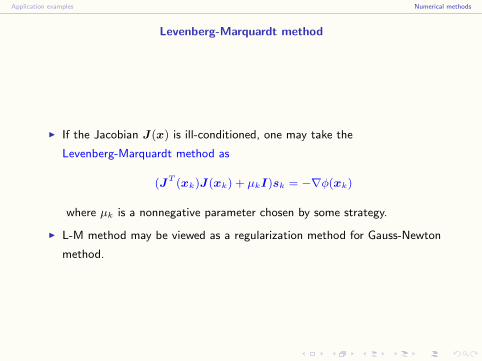
Levenberg-Marquardt method
I If the Jacobian J(x) is ill-conditioned, one may take the
Levenberg-Marquardt method as
(JT (xk)J(xk) + µkI)sk = −∇φ(xk)
where µk is a nonnegative parameter chosen by some strategy.
I L-M method may be viewed as a regularization method for Gauss-Newton
method.
Application examples Numerical methods
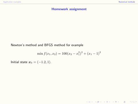
Homework assignment
Newton’s method and BFGS method for example
min f(x1, x2) = 100(x2 − x21)
2 + (x1 − 1)2
Initial state x0 = (−1.2, 1).

Application examples Numerical methods
References
1. /�©§�Æ�§¢^�`z�{§�ënó�ÆÑ��§1n
�§2004"
2. J.F. Bonnans et al., Numerical optimization: Theoretical and practical
aspects, Universitext, Springer, Berlin, 2003.
![Nonlinear Programming Models Fabio Schoen Introductionfor all x,y ∈ Ω,λ ∈ [0,1] Nonlinear Programming Models – p. 5 Convex Functions x y Nonlinear Programming Models – p.](https://static.fdocuments.in/doc/165x107/60025c042470c9743d105bb3/nonlinear-programming-models-fabio-schoen-for-all-xy-a-a-01-nonlinear.jpg)