Lecture 7: Introduction to MIMO Systems
85
The University of Newcastle ELEC4410 Control System Design Lecture 7: Introduction to MIMO Systems School of Electrical Engineering and Computer Science The University of Newcastle Lecture 7: Introduction to MIMO Systems – p. 1/35
Transcript of Lecture 7: Introduction to MIMO Systems
The University of Newcastle
ELEC4410
Control System Design
Lecture 7: Introduction to MIMO Systems
School of Electrical Engineering and Computer Science
The University of Newcastle
Lecture 7: Introduction to MIMO Systems – p. 1/35

The University of Newcastle
Outline
MIMO Systems
Lecture 7: Introduction to MIMO Systems – p. 2/35

The University of Newcastle
Outline
MIMO Systems
Transfer Matrices, Poles and Zeros
Lecture 7: Introduction to MIMO Systems – p. 2/35

The University of Newcastle
Outline
MIMO Systems
Transfer Matrices, Poles and Zeros
Stability
Lecture 7: Introduction to MIMO Systems – p. 2/35
The University of Newcastle
Outline
MIMO Systems
Transfer Matrices, Poles and Zeros
Stability
Interaction, Decoupling and Diagonal Dominance
Lecture 7: Introduction to MIMO Systems – p. 2/35

The University of Newcastle
Outline
MIMO Systems
Transfer Matrices, Poles and Zeros
Stability
Interaction, Decoupling and Diagonal Dominance
Sensitivities, Performance and Robustness
Lecture 7: Introduction to MIMO Systems – p. 2/35
The University of Newcastle
Outline
MIMO Systems
Transfer Matrices, Poles and Zeros
Stability
Interaction, Decoupling and Diagonal Dominance
Sensitivities, Performance and Robustness
MIMO IMC Control
Lecture 7: Introduction to MIMO Systems – p. 2/35
The University of Newcastle
Outline
MIMO Systems
Transfer Matrices, Poles and Zeros
Stability
Interaction, Decoupling and Diagonal Dominance
Sensitivities, Performance and Robustness
MIMO IMC Control
References: Control System Design, Goodwin, Graebe &
Salgado.
Multivariable Feedback Control: Analysis and Design, Skogestad
& Postlethwaite.
Lecture 7: Introduction to MIMO Systems – p. 2/35
The University of Newcastle
MIMO Systems
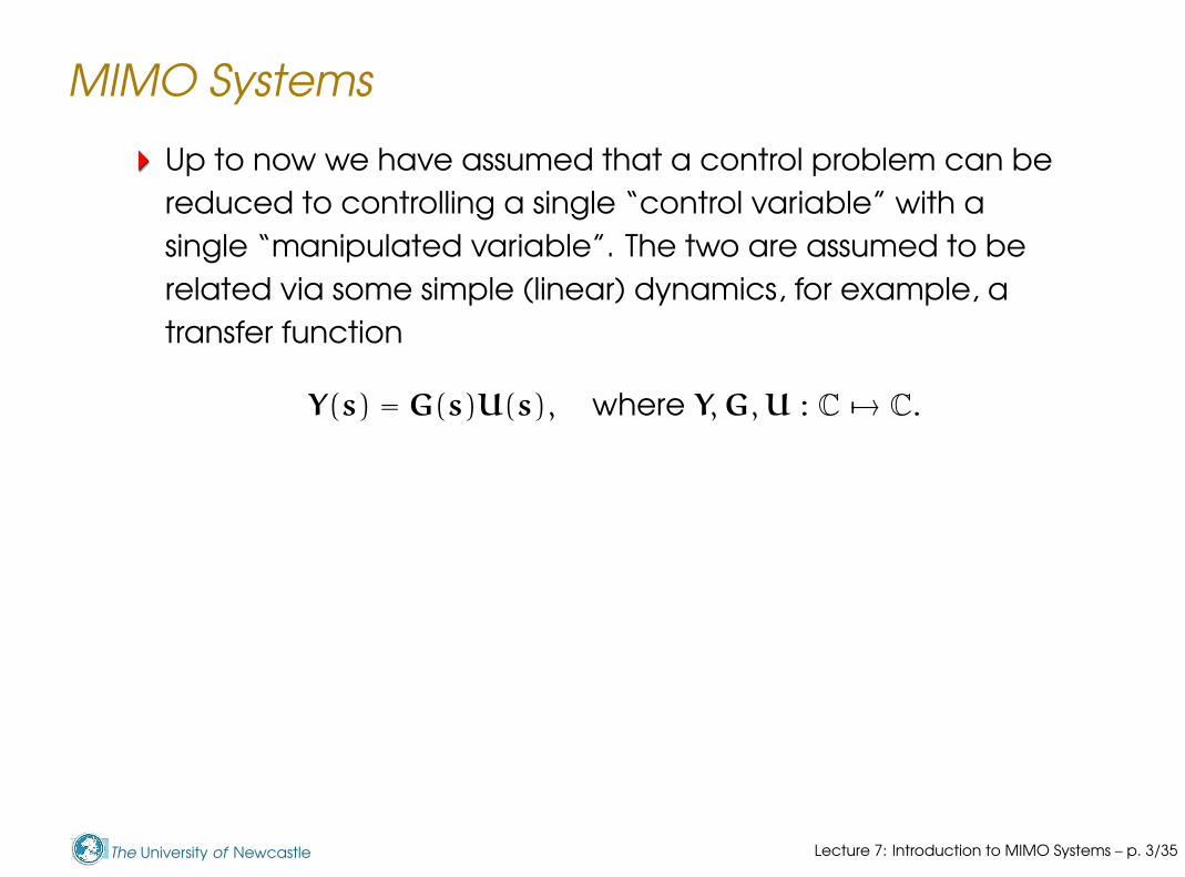
Up to now we have assumed that a control problem can be
reduced to controlling a single “control variable” with a
single “manipulated variable”. The two are assumed to be
related via some simple (linear) dynamics, for example, a
transfer function
Y(s) = G(s)U(s), where Y, G, U : C 7→ C.
Lecture 7: Introduction to MIMO Systems – p. 3/35

The University of Newcastle
MIMO Systems
Up to now we have assumed that a control problem can be
reduced to controlling a single “control variable” with a
single “manipulated variable”. The two are assumed to be
related via some simple (linear) dynamics, for example, a
transfer function
Y(s) = G(s)U(s), where Y, G, U : C 7→ C.
However, in most cases, a system has more than one
manipulated variable and more than one control input, and
the interactions between these are such that the model
cannot be further reduced.
A system in which the input and the output are vectors,
rather than scalars, is a system with Multiple Inputs and
Multiple Outputs (a MIMO system), sometimes also called a
multivariable system.
Lecture 7: Introduction to MIMO Systems – p. 3/35

The University of Newcastle
Example: Control of an Aircraft
Wilbur Wright said in 1901:
Men know how to construct airplanes. Men also know how to
build engines. Inability to balance and steer still confronts
students on the flying problem. When this one feature has been
worked out, the age of flying will have arrived, for all other
difficulties are of minor importance.
Lecture 7: Introduction to MIMO Systems – p. 4/35

The University of Newcastle
Example: Control of an Aircraft
Wilbur Wright said in 1901:
Men know how to construct airplanes. Men also know how to
build engines. Inability to balance and steer still confronts
students on the flying problem. When this one feature has been
worked out, the age of flying will have arrived, for all other
difficulties are of minor importance.
The Wright Brothers
solved the control problem
and flew the Kitty Hawk
on december 17, 1903.
Lecture 7: Introduction to MIMO Systems – p. 4/35
The University of Newcastle
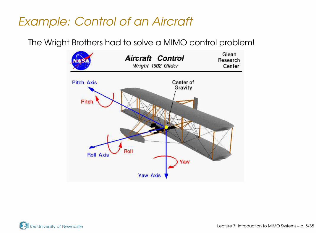
Example: Control of an Aircraft
The Wright Brothers had to solve a MIMO control problem!
Lecture 7: Introduction to MIMO Systems – p. 5/35

The University of Newcastle
Example: Copper Heap Bioleaching
Heap bioleaching is a process used to extract copper and other
metals from large amounts of heaped ore with low grade
content, based on the action of chemolithotrophic bacteria.
Lecture 7: Introduction to MIMO Systems – p. 6/35
The University of Newcastle
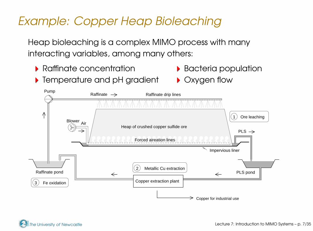
Example: Copper Heap Bioleaching
Heap bioleaching is a complex MIMO process with many
interacting variables, among many others:
Raffinate concentration Bacteria population
Temperature and pH gradient Oxygen flow
Copper for industrial use
PumpRaffinate drip lines
Raffinate pond
Copper extraction plant
Impervious liner
PLS pond2 Metallic Cu extraction
1 Ore leaching
3 Fe oxidation
Raffinate
AirBlowerHeap of crushed copper sulfide ore
Forced aireation lines
PLS
Lecture 7: Introduction to MIMO Systems – p. 7/35
The University of Newcastle
Transfer Matrices
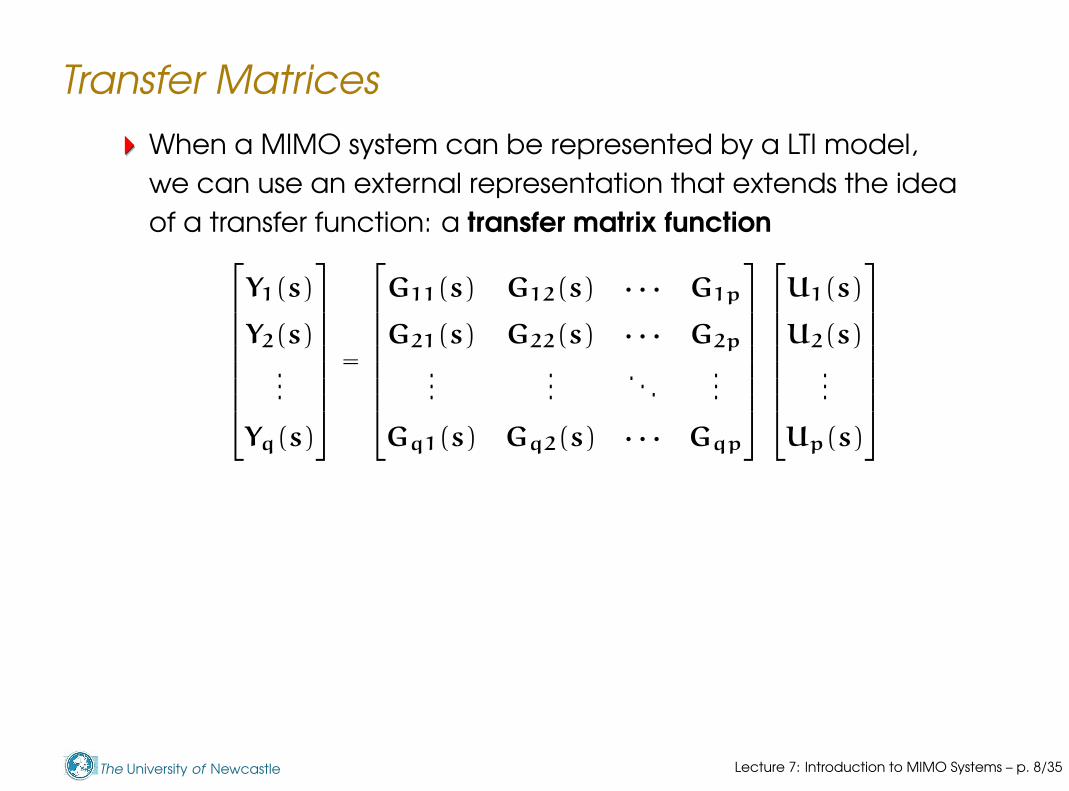
When a MIMO system can be represented by a LTI model,
we can use an external representation that extends the idea
of a transfer function: a transfer matrix function
Y1(s)
Y2(s)
...
Yq(s)
=
G11(s) G12(s) · · · G1p
G21(s) G22(s) · · · G2p
......
. . ....
Gq1(s) Gq2(s) · · · Gqp
U1(s)
U2(s)
...
Up(s)
Lecture 7: Introduction to MIMO Systems – p. 8/35

The University of Newcastle
Transfer Matrices
When a MIMO system can be represented by a LTI model,
we can use an external representation that extends the idea
of a transfer function: a transfer matrix function
Y1(s)
Y2(s)
...
Yq(s)
=
G11(s) G12(s) · · · G1p
G21(s) G22(s) · · · G2p
......
. . ....
Gq1(s) Gq2(s) · · · Gqp
U1(s)
U2(s)
...
Up(s)
We can still write
Y(s) = G(s)U(s),
but now Y ∈ Cq, U ∈ C
p, and G ∈ Cq×p. Besides gain and
phase in G(s), for MIMO systems also directions play a
fundamental role.
Lecture 7: Introduction to MIMO Systems – p. 8/35
The University of Newcastle
Example: Four Tank Apparatus
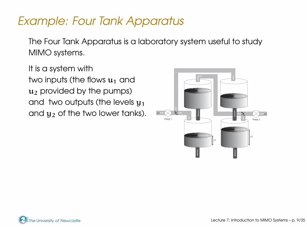
The Four Tank Apparatus is a laboratory system useful to study
MIMO systems.
It is a system with
two inputs (the flows u1 and
u2 provided by the pumps)
and two outputs (the levels y1
and y2 of the two lower tanks).
Lecture 7: Introduction to MIMO Systems – p. 9/35
The University of Newcastle
Example: Four Tank Apparatus
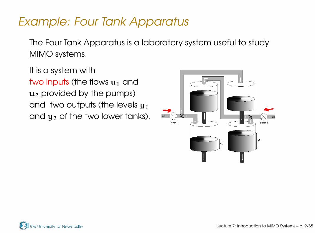
The Four Tank Apparatus is a laboratory system useful to study
MIMO systems.
It is a system with
two inputs (the flows u1 and
u2 provided by the pumps)
and two outputs (the levels y1
and y2 of the two lower tanks).
Lecture 7: Introduction to MIMO Systems – p. 9/35

The University of Newcastle
Example: Four Tank Apparatus
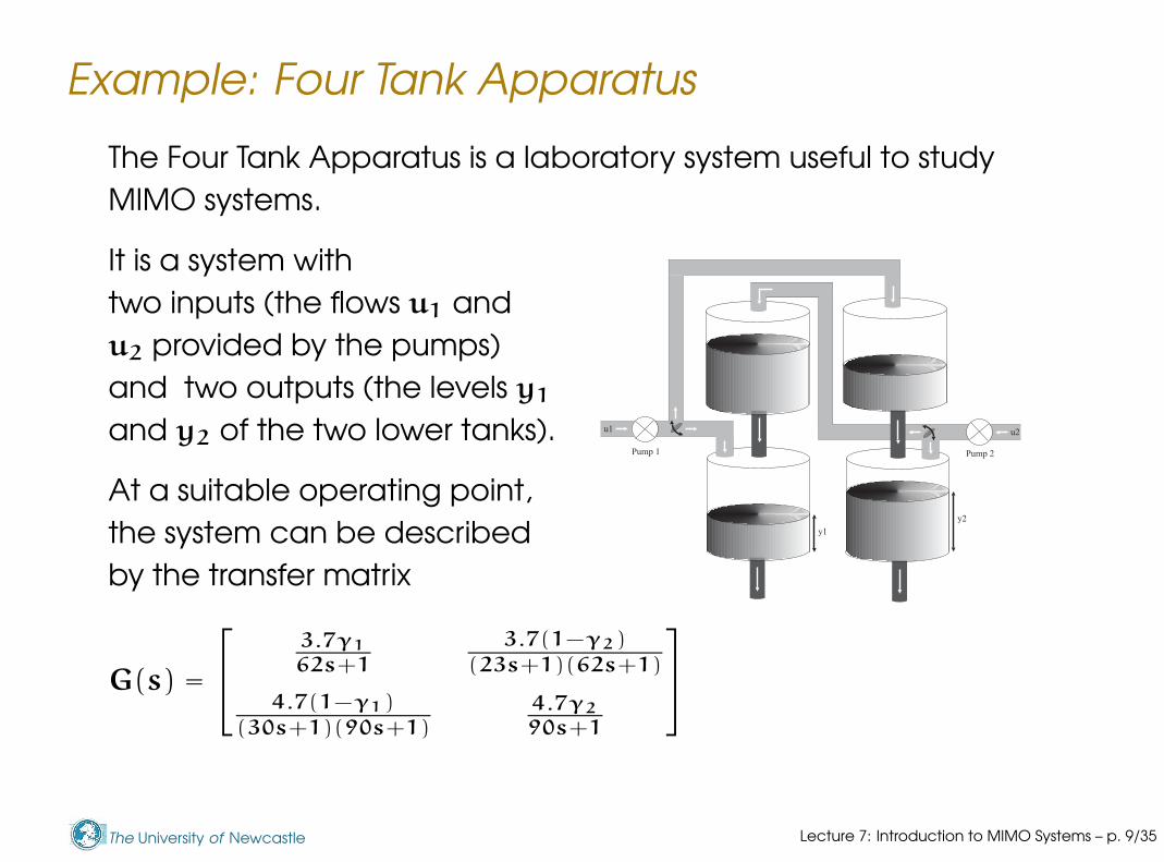
The Four Tank Apparatus is a laboratory system useful to study
MIMO systems.
It is a system with
two inputs (the flows u1 and
u2 provided by the pumps)
and two outputs (the levels y1
and y2 of the two lower tanks).
Lecture 7: Introduction to MIMO Systems – p. 9/35
The University of Newcastle
Example: Four Tank Apparatus
The Four Tank Apparatus is a laboratory system useful to study
MIMO systems.
It is a system with
two inputs (the flows u1 and
u2 provided by the pumps)
and two outputs (the levels y1
and y2 of the two lower tanks).
At a suitable operating point,
the system can be described
by the transfer matrix
G(s) =
3.7γ1
62s+1
3.7(1−γ2)
(23s+1)(62s+1)
4.7(1−γ1)
(30s+1)(90s+1)
4.7γ2
90s+1
Lecture 7: Introduction to MIMO Systems – p. 9/35
The University of Newcastle
Poles of a MIMO System
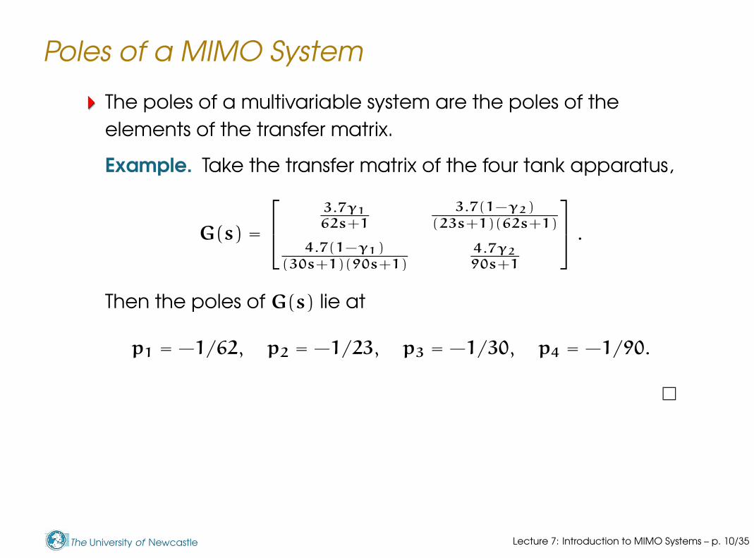
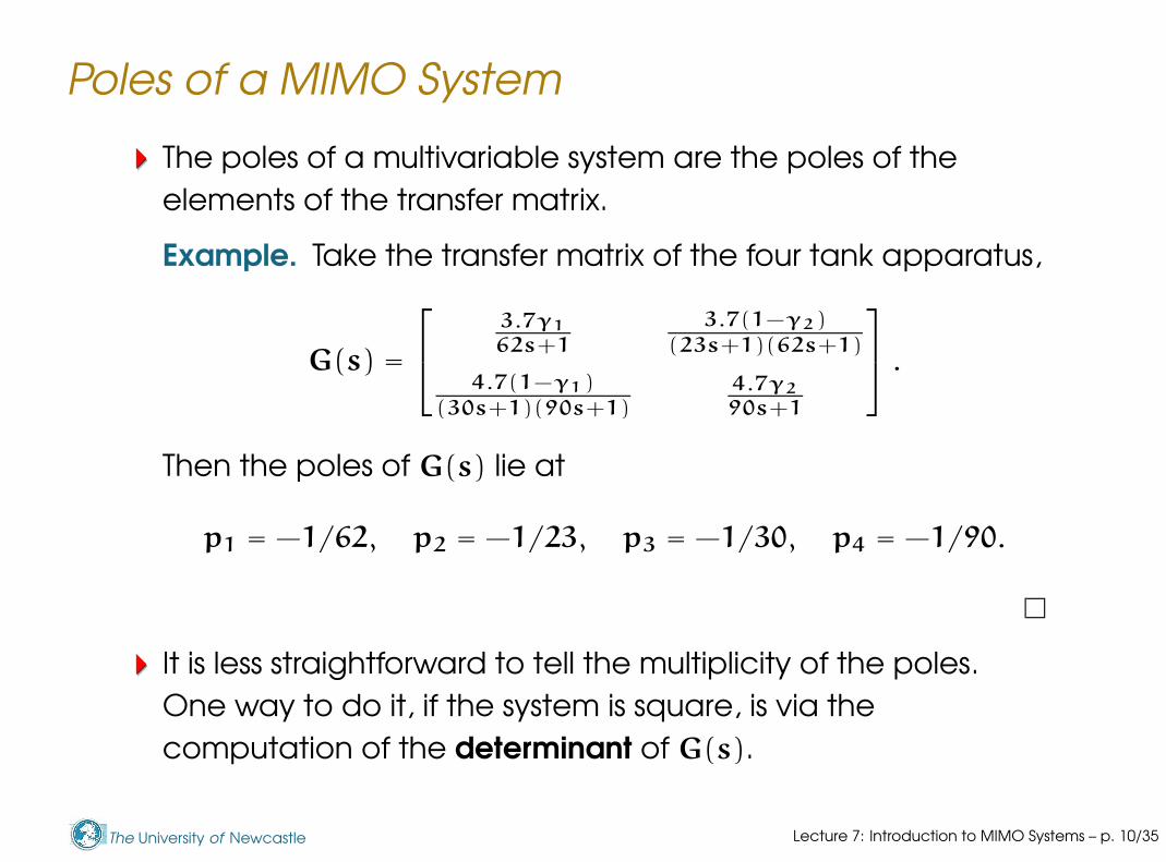
The poles of a multivariable system are the poles of the
elements of the transfer matrix.
Example. Take the transfer matrix of the four tank apparatus,
G(s) =
3.7γ1
62s+1
3.7(1−γ2)
(23s+1)(62s+1)
4.7(1−γ1)
(30s+1)(90s+1)
4.7γ2
90s+1
.
Then the poles of G(s) lie at
p1 = −1/62, p2 = −1/23, p3 = −1/30, p4 = −1/90.
Lecture 7: Introduction to MIMO Systems – p. 10/35
The University of Newcastle
Poles of a MIMO System
The poles of a multivariable system are the poles of the
elements of the transfer matrix.
Example. Take the transfer matrix of the four tank apparatus,
G(s) =
3.7γ1
62s+1
3.7(1−γ2)
(23s+1)(62s+1)
4.7(1−γ1)
(30s+1)(90s+1)
4.7γ2
90s+1
.
Then the poles of G(s) lie at
p1 = −1/62, p2 = −1/23, p3 = −1/30, p4 = −1/90.
It is less straightforward to tell the multiplicity of the poles.
One way to do it, if the system is square, is via the
computation of the determinant of G(s).
Lecture 7: Introduction to MIMO Systems – p. 10/35
The University of Newcastle
Poles of a MIMO System
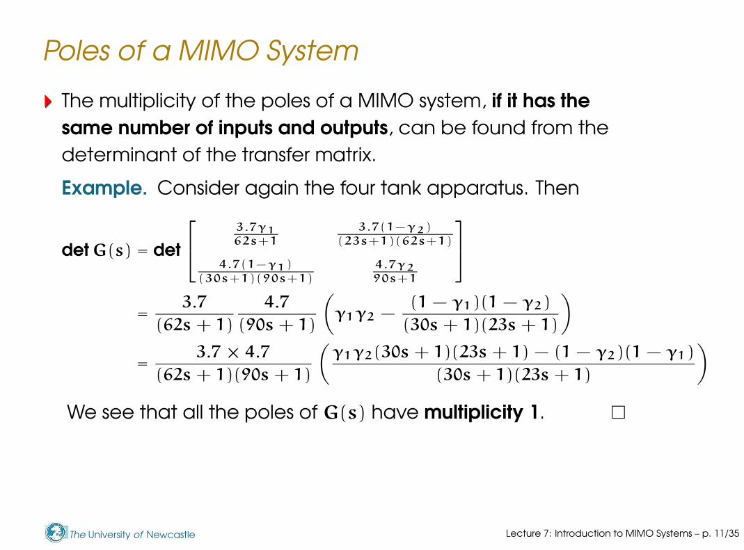
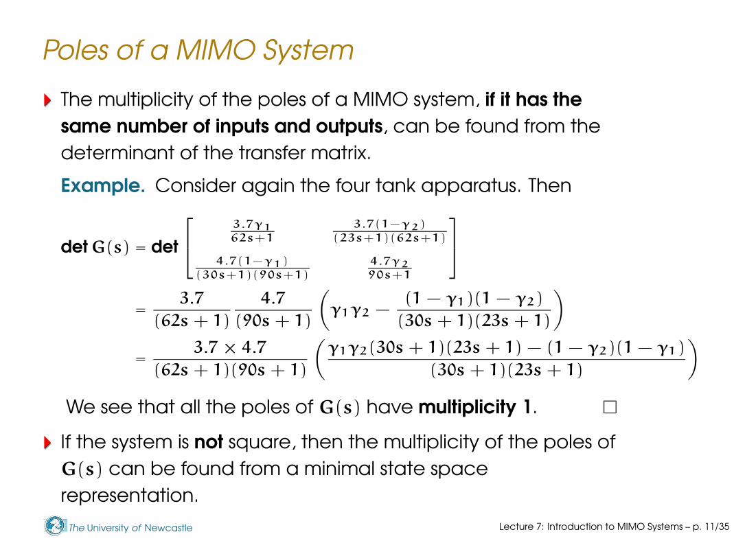
The multiplicity of the poles of a MIMO system, if it has the
same number of inputs and outputs, can be found from the
determinant of the transfer matrix.
Example. Consider again the four tank apparatus. Then
det G(s) = det
3.7γ1
62s+1
3.7(1−γ2)
(23s+1)(62s+1)
4.7(1−γ1)
(30s+1)(90s+1)
4.7γ2
90s+1
=3.7
(62s + 1)
4.7
(90s + 1)
(
γ1γ2 −(1 − γ1)(1 − γ2)
(30s + 1)(23s + 1)
)
=3.7 × 4.7
(62s + 1)(90s + 1)
(
γ1γ2(30s + 1)(23s + 1) − (1 − γ2)(1 − γ1)
(30s + 1)(23s + 1)
)
We see that all the poles of G(s) have multiplicity 1.
Lecture 7: Introduction to MIMO Systems – p. 11/35
The University of Newcastle
Poles of a MIMO System
The multiplicity of the poles of a MIMO system, if it has the
same number of inputs and outputs, can be found from the
determinant of the transfer matrix.
Example. Consider again the four tank apparatus. Then
det G(s) = det
3.7γ1
62s+1
3.7(1−γ2)
(23s+1)(62s+1)
4.7(1−γ1)
(30s+1)(90s+1)
4.7γ2
90s+1
=3.7
(62s + 1)
4.7
(90s + 1)
(
γ1γ2 −(1 − γ1)(1 − γ2)
(30s + 1)(23s + 1)
)
=3.7 × 4.7
(62s + 1)(90s + 1)
(
γ1γ2(30s + 1)(23s + 1) − (1 − γ2)(1 − γ1)
(30s + 1)(23s + 1)
)
We see that all the poles of G(s) have multiplicity 1.
If the system is not square, then the multiplicity of the poles of
G(s) can be found from a minimal state space
representation.
Lecture 7: Introduction to MIMO Systems – p. 11/35
The University of Newcastle
Poles of a MIMO System
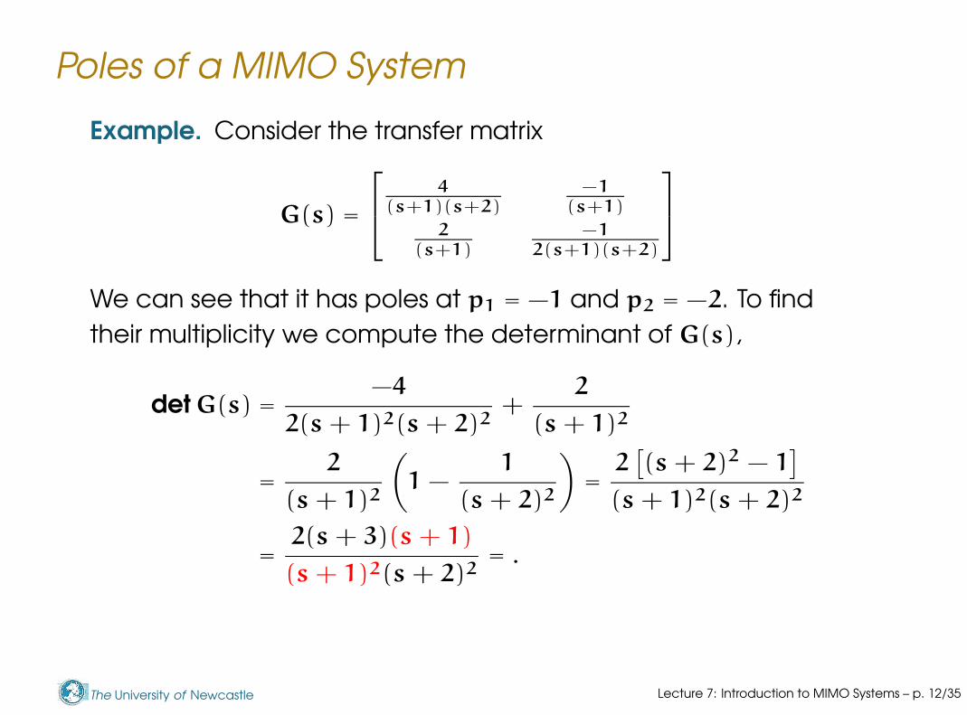
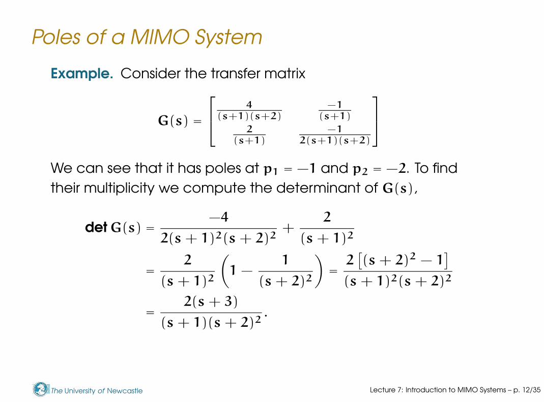
Example. Consider the transfer matrix
G(s) =
4(s+1)(s+2)
−1(s+1)
2(s+1)
−12(s+1)(s+2)
We can see that it has poles at p1 = −1 and p2 = −2. To find
their multiplicity we compute the determinant of G(s),
det G(s) =−4
2(s + 1)2(s + 2)2+
2
(s + 1)2
=2
(s + 1)2
(
1 −1
(s + 2)2
)
=2
[
(s + 2)2 − 1]
(s + 1)2(s + 2)2
=2(s + 3)(s + 1)
(s + 1)2(s + 2)2= .
Lecture 7: Introduction to MIMO Systems – p. 12/35
The University of Newcastle
Poles of a MIMO System
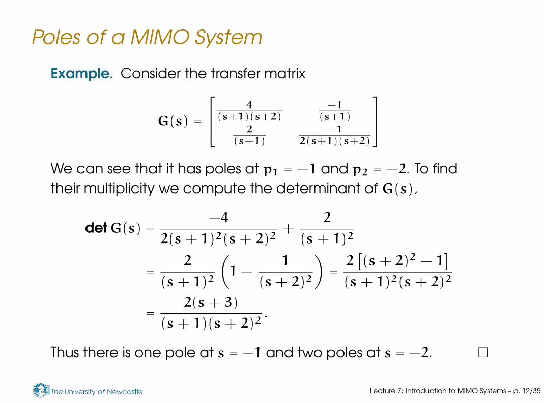
Example. Consider the transfer matrix
G(s) =
4(s+1)(s+2)
−1(s+1)
2(s+1)
−12(s+1)(s+2)
We can see that it has poles at p1 = −1 and p2 = −2. To find
their multiplicity we compute the determinant of G(s),
det G(s) =−4
2(s + 1)2(s + 2)2+
2
(s + 1)2
=2
(s + 1)2
(
1 −1
(s + 2)2
)
=2
[
(s + 2)2 − 1]
(s + 1)2(s + 2)2
=2(s + 3)
(s + 1)(s + 2)2.
Lecture 7: Introduction to MIMO Systems – p. 12/35
The University of Newcastle
Poles of a MIMO System
Example. Consider the transfer matrix
G(s) =
4(s+1)(s+2)
−1(s+1)
2(s+1)
−12(s+1)(s+2)
We can see that it has poles at p1 = −1 and p2 = −2. To find
their multiplicity we compute the determinant of G(s),
det G(s) =−4
2(s + 1)2(s + 2)2+
2
(s + 1)2
=2
(s + 1)2
(
1 −1
(s + 2)2
)
=2
[
(s + 2)2 − 1]
(s + 1)2(s + 2)2
=2(s + 3)
(s + 1)(s + 2)2.
Thus there is one pole at s = −1 and two poles at s = −2.
Lecture 7: Introduction to MIMO Systems – p. 12/35
The University of Newcastle
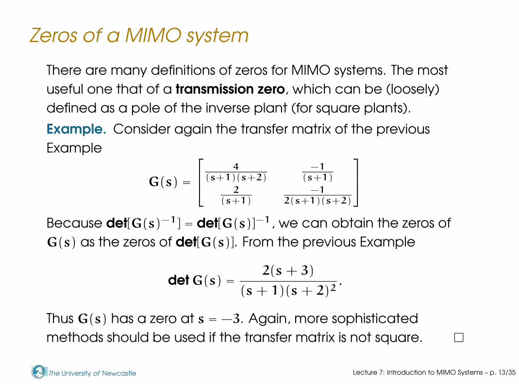
Zeros of a MIMO system
There are many definitions of zeros for MIMO systems. The most
useful one that of a transmission zero, which can be (loosely)
defined as a pole of the inverse plant (for square plants).
Example. Consider again the transfer matrix of the previous
Example
G(s) =
4(s+1)(s+2)
−1(s+1)
2(s+1)
−12(s+1)(s+2)
Because det[G(s)−1] = det[G(s)]−1, we can obtain the zeros of
G(s) as the zeros of det[G(s)]. From the previous Example
det G(s) =2(s + 3)
(s + 1)(s + 2)2.
Thus G(s) has a zero at s = −3. Again, more sophisticated
methods should be used if the transfer matrix is not square.
Lecture 7: Introduction to MIMO Systems – p. 13/35

The University of Newcastle
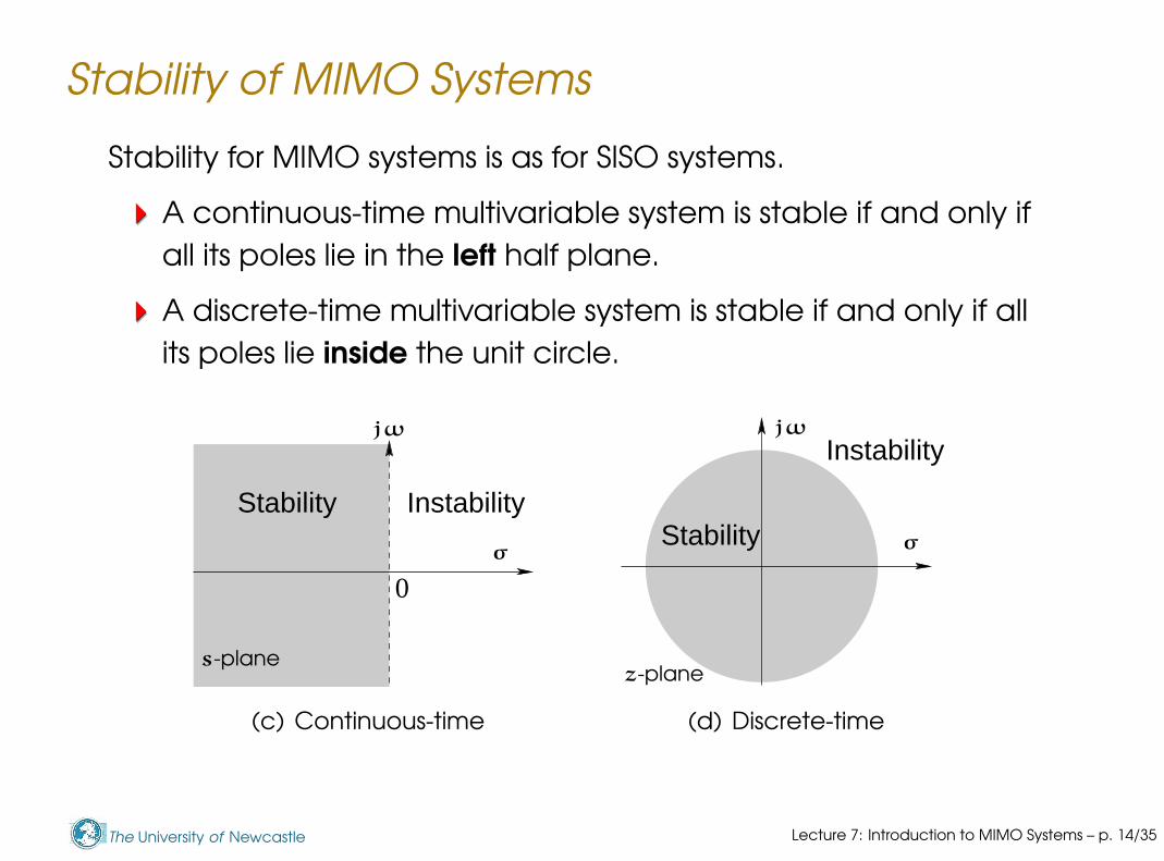
Stability of MIMO Systems
Stability for MIMO systems is as for SISO systems.
A continuous-time multivariable system is stable if and only if
all its poles lie in the left half plane.
InstabilityStability
0
jω
σ
s-plane
(a) Continuous-time
Lecture 7: Introduction to MIMO Systems – p. 14/35
The University of Newcastle
Stability of MIMO Systems
Stability for MIMO systems is as for SISO systems.
A continuous-time multivariable system is stable if and only if
all its poles lie in the left half plane.
A discrete-time multivariable system is stable if and only if all
its poles lie inside the unit circle.
InstabilityStability
0
jω
σ
s-plane
(c) Continuous-time
Instability
Stability
z-plane
σ
jω
(d) Discrete-time
Lecture 7: Introduction to MIMO Systems – p. 14/35
The University of Newcastle
Minimum Phase MIMO Systems
As for a SISO system, a MIMO system is said to be minimum phase
if it has no zeros outside the stability region. Otherwise, it is called
nonminimum phase.
A continuous-time multivariable system is minimum phase if
all its zeros lie in the left half plane.
Lecture 7: Introduction to MIMO Systems – p. 15/35
The University of Newcastle
Minimum Phase MIMO Systems
As for a SISO system, a MIMO system is said to be minimum phase
if it has no zeros outside the stability region. Otherwise, it is called
nonminimum phase.
A continuous-time multivariable system is minimum phase if
all its zeros lie in the left half plane.
A discrete-time multivariable system is minimum phase if all its
zeros lie inside the unit circle.
Lecture 7: Introduction to MIMO Systems – p. 15/35
The University of Newcastle
Minimum Phase MIMO Systems
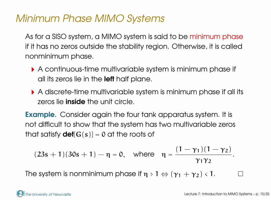
As for a SISO system, a MIMO system is said to be minimum phase
if it has no zeros outside the stability region. Otherwise, it is called
nonminimum phase.
A continuous-time multivariable system is minimum phase if
all its zeros lie in the left half plane.
A discrete-time multivariable system is minimum phase if all its
zeros lie inside the unit circle.
Example. Consider again the four tank apparatus system. It is
not difficult to show that the system has two multivariable zeros
that satisfy det[G(s)] = 0 at the roots of
(23s + 1)(30s + 1) − η = 0, where η =(1 − γ1)(1 − γ2)
γ1γ2
.
The system is nonminimum phase if η > 1 ⇔ (γ1 + γ2) < 1.
Lecture 7: Introduction to MIMO Systems – p. 15/35
The University of Newcastle
Interaction and Decoupling
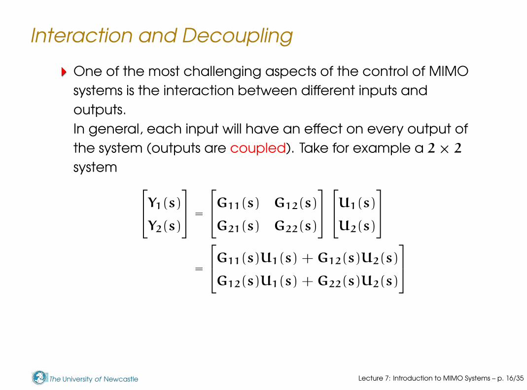
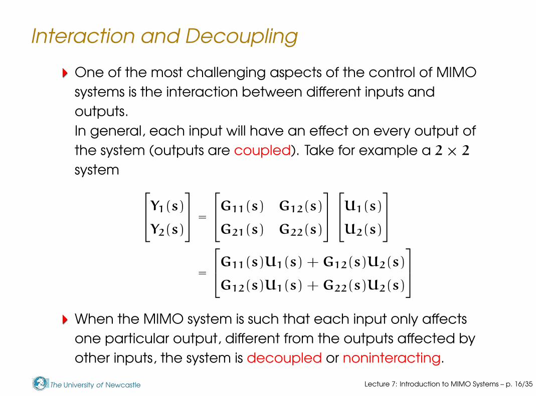
One of the most challenging aspects of the control of MIMO
systems is the interaction between different inputs and
outputs.
In general, each input will have an effect on every output of
the system (outputs are coupled). Take for example a 2 × 2
system
Y1(s)
Y2(s)
=
G11(s) G12(s)
G21(s) G22(s)
U1(s)
U2(s)
=
G11(s)U1(s) + G12(s)U2(s)
G12(s)U1(s) + G22(s)U2(s)
Lecture 7: Introduction to MIMO Systems – p. 16/35
The University of Newcastle
Interaction and Decoupling
One of the most challenging aspects of the control of MIMO
systems is the interaction between different inputs and
outputs.
In general, each input will have an effect on every output of
the system (outputs are coupled). Take for example a 2 × 2
system
Y1(s)
Y2(s)
=
G11(s) G12(s)
G21(s) G22(s)
U1(s)
U2(s)
=
G11(s)U1(s) + G12(s)U2(s)
G12(s)U1(s) + G22(s)U2(s)
When the MIMO system is such that each input only affects
one particular output, different from the outputs affected by
other inputs, the system is decoupled or noninteracting.
Lecture 7: Introduction to MIMO Systems – p. 16/35

The University of Newcastle
Interaction and Decoupling
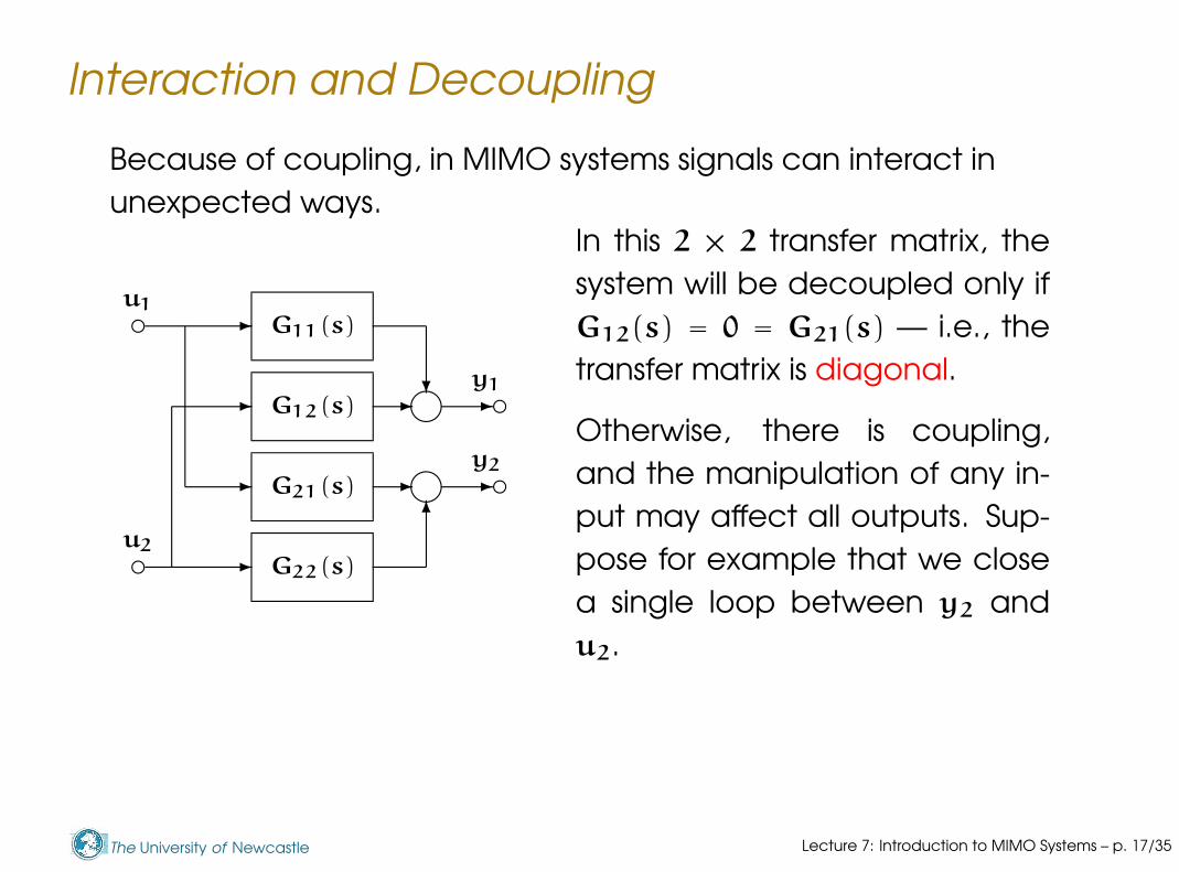
Because of coupling, in MIMO systems signals can interact in
unexpected ways.
G12(s)
G11(s)u1
u2
G22(s)
G21(s)y2
y1i
i
c
c
c
c
-
-
- ?
-
-
-
6
-
-
In this 2 × 2 transfer matrix, the
system will be decoupled only if
G12(s) = 0 = G21(s) — i.e., the
transfer matrix is diagonal.
Lecture 7: Introduction to MIMO Systems – p. 17/35
The University of Newcastle
Interaction and Decoupling
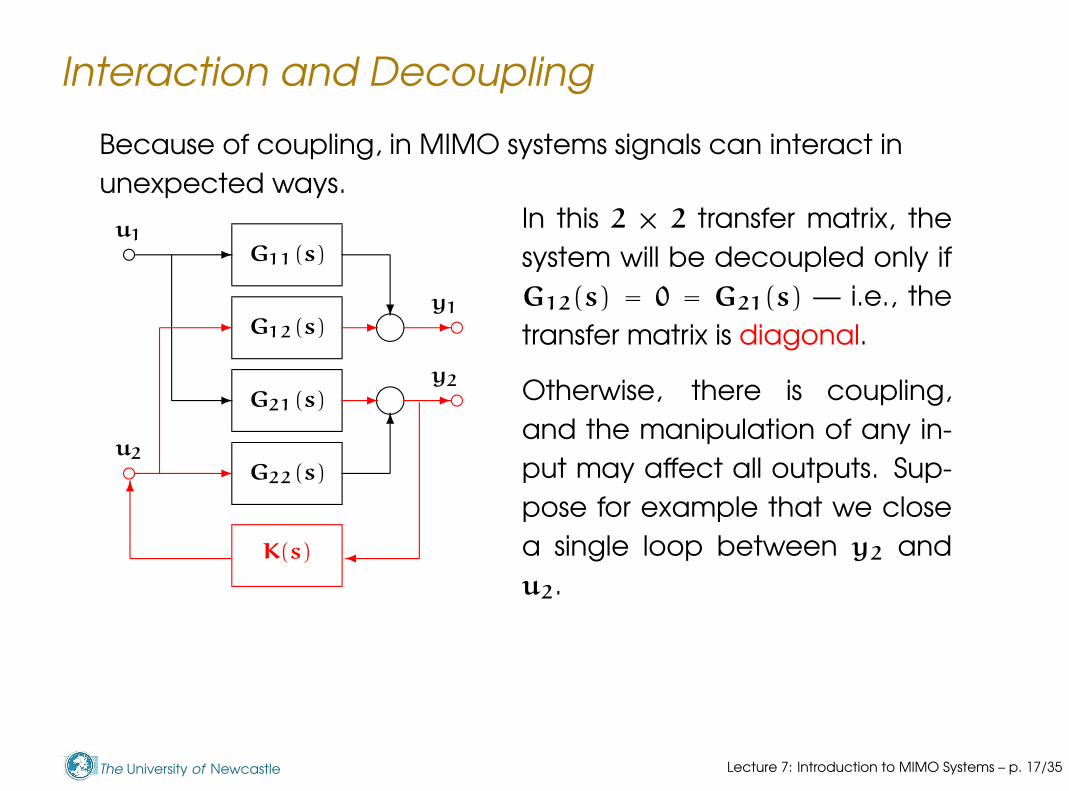
Because of coupling, in MIMO systems signals can interact in
unexpected ways.
G12(s)
G11(s)u1
u2
G22(s)
G21(s)y2
y1i
i
c
c
c
c
-
-
- ?
-
-
-
6
-
-
In this 2 × 2 transfer matrix, the
system will be decoupled only if
G12(s) = 0 = G21(s) — i.e., the
transfer matrix is diagonal.
Otherwise, there is coupling,
and the manipulation of any in-
put may affect all outputs. Sup-
pose for example that we close
a single loop between y2 and
u2.
Lecture 7: Introduction to MIMO Systems – p. 17/35
The University of Newcastle
Interaction and Decoupling
Because of coupling, in MIMO systems signals can interact in
unexpected ways.
G12(s)
G11(s)u1
u2
G22(s)
G21(s)y2
y1
K(s)
i
i
c
c
c
c
-
-
?
6
¾
6-
- -
- -
-
In this 2 × 2 transfer matrix, the
system will be decoupled only if
G12(s) = 0 = G21(s) — i.e., the
transfer matrix is diagonal.
Otherwise, there is coupling,
and the manipulation of any in-
put may affect all outputs. Sup-
pose for example that we close
a single loop between y2 and
u2.
Lecture 7: Introduction to MIMO Systems – p. 17/35

The University of Newcastle
Interaction and Decoupling
Because of coupling, in MIMO systems signals can interact in
unexpected ways.
G12(s)
G11(s)u1
u2
G22(s)
G21(s)y2
y1
K(s)
i
i
c
c
c
c
-
-
?
6
¾
6-
- -
- -
-
In this 2 × 2 transfer matrix, the
system will be decoupled only if
G12(s) = 0 = G21(s) — i.e., the
transfer matrix is diagonal.
Otherwise, there is coupling,
and the manipulation of any in-
put may affect all outputs. Sup-
pose for example that we close
a single loop between y2 and
u2.
Both outputs will be affected!
Lecture 7: Introduction to MIMO Systems – p. 17/35
The University of Newcastle
Interaction and Decoupling
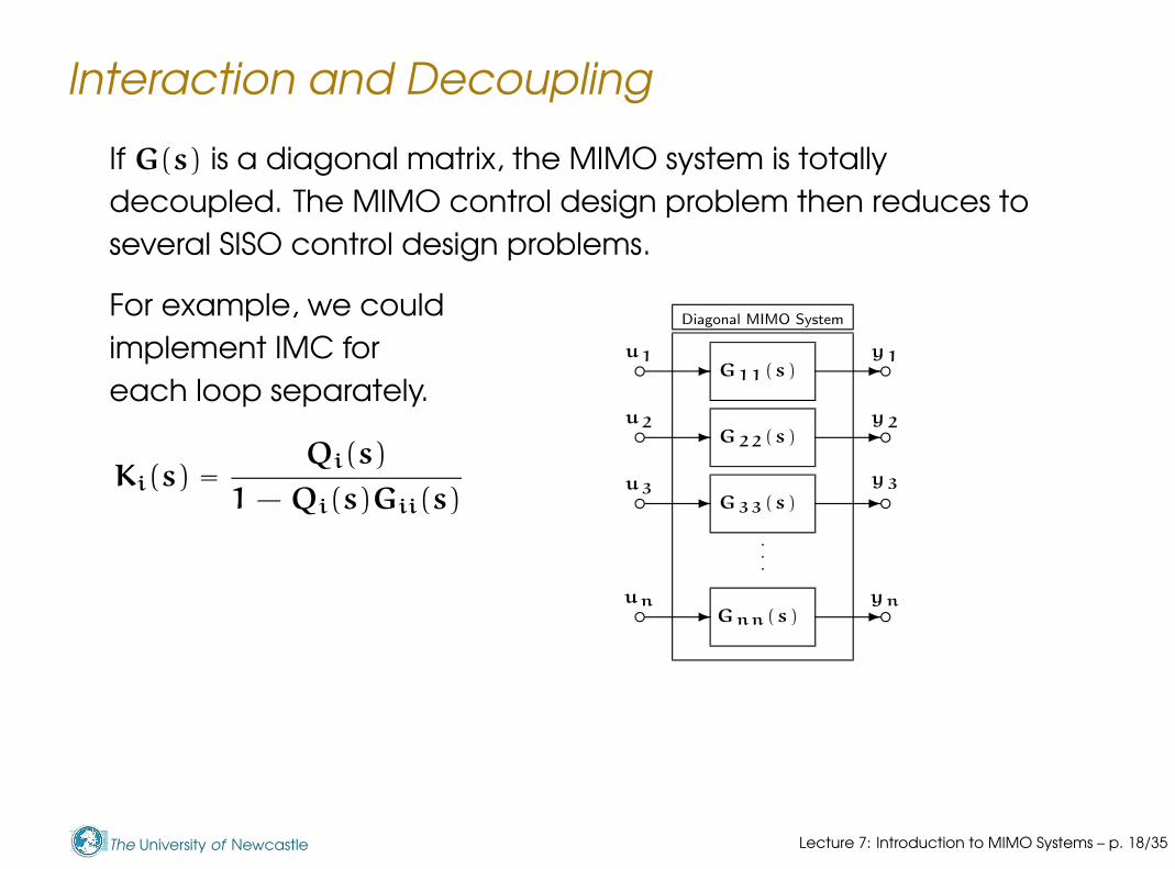
If G(s) is a diagonal matrix, the MIMO system is totally
decoupled. The MIMO control design problem then reduces to
several SISO control design problems.
For example, we could
b b
b b
b b
b b
- -
- -
- -
- -
.
.
.
Gnn(s)
G33(s)
G22(s)
G11(s)y1
y2
y3
yn
u1
u2
u3
un
Diagonal MIMO System
implement IMC for
each loop separately.
Ki(s) =Qi(s)
1 − Qi(s)Gii(s)
Lecture 7: Introduction to MIMO Systems – p. 18/35

The University of Newcastle
Interaction and Decoupling
If G(s) is a diagonal matrix, the MIMO system is totally
decoupled. The MIMO control design problem then reduces to
several SISO control design problems.
For example, we could
b b
b b
b b
b b-
-
-
--
-
-
-
- -
- -
- -
- -
Kn(s)
K3(s)
K2(s)
K1(s)
.
.
.
Gnn(s)
G33(s)
G22(s)
G11(s)y1
y2
y3
yn
u1
u2
u3
un
.
.
.
Diagonal MIMO System
implement IMC for
each loop separately.
Ki(s) =Qi(s)
1 − Qi(s)Gii(s)
Lecture 7: Introduction to MIMO Systems – p. 18/35

The University of Newcastle
Diagonal Dominance
Non-diagonal plants cannot, in general, be approached as
a multiple SISO problem, because of coupling. However, in
some cases a plant is sufficiently diagonal, which still makes it
easier to control.
Lecture 7: Introduction to MIMO Systems – p. 19/35
The University of Newcastle
Diagonal Dominance
Non-diagonal plants cannot, in general, be approached as
a multiple SISO problem, because of coupling. However, in
some cases a plant is sufficiently diagonal, which still makes it
easier to control.
Loosely, a diagonally dominant plant has a transfer matrix in
which the transfer functions on the diagonal are greater in
magnitude than the off-diagonal elements.
Lecture 7: Introduction to MIMO Systems – p. 19/35

The University of Newcastle
Diagonal Dominance
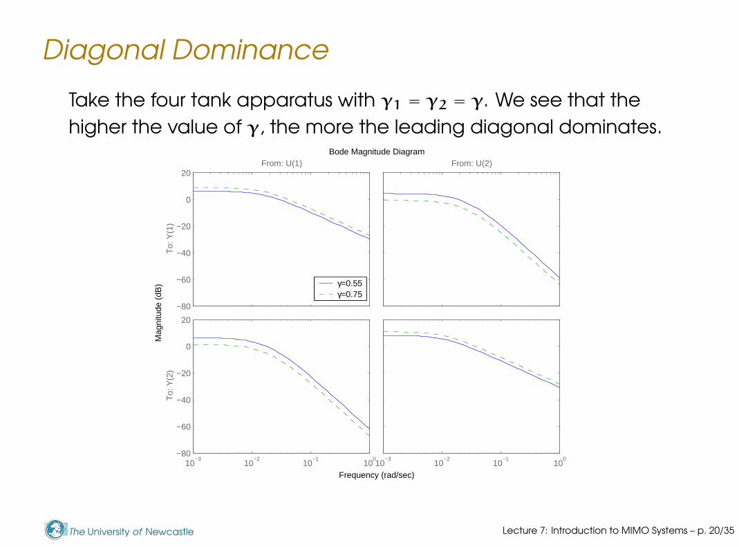
Take the four tank apparatus with γ1 = γ2 = γ. We see that the
higher the value of γ, the more the leading diagonal dominates.Bode Magnitude Diagram
Frequency (rad/sec)
Mag
nitu
de (
dB)
−60
−40
−20
0
20From: U(1)
To:
Y(1
)
γ=0.55
10−3
10−2
10−1
100
−80
−60
−40
−20
0
20
To:
Y(2
)From: U(2)
10−3
10−2
10−1
100
Lecture 7: Introduction to MIMO Systems – p. 20/35
The University of Newcastle
Diagonal Dominance
Take the four tank apparatus with γ1 = γ2 = γ. We see that the
higher the value of γ, the more the leading diagonal dominates.Bode Magnitude Diagram
Frequency (rad/sec)
Mag
nitu
de (
dB)
−80
−60
−40
−20
0
20From: U(1)
To:
Y(1
)
γ=0.55γ=0.75
10−3
10−2
10−1
100
−80
−60
−40
−20
0
20
To:
Y(2
)From: U(2)
10−3
10−2
10−1
100
Lecture 7: Introduction to MIMO Systems – p. 20/35
The University of Newcastle
Diagonal Dominance
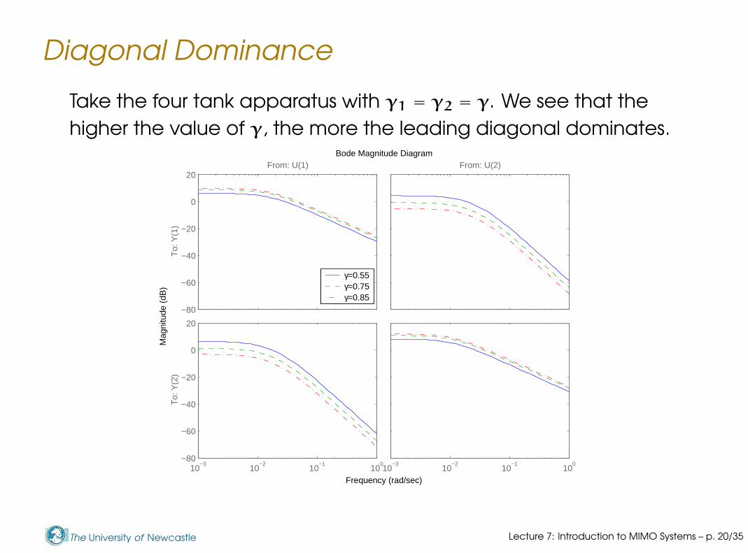
Take the four tank apparatus with γ1 = γ2 = γ. We see that the
higher the value of γ, the more the leading diagonal dominates.Bode Magnitude Diagram
Frequency (rad/sec)
Mag
nitu
de (
dB)
−80
−60
−40
−20
0
20From: U(1)
To:
Y(1
)
γ=0.55γ=0.75γ=0.85
10−3
10−2
10−1
100
−80
−60
−40
−20
0
20
To:
Y(2
)From: U(2)
10−3
10−2
10−1
100
Lecture 7: Introduction to MIMO Systems – p. 20/35

The University of Newcastle
Diagonal Dominance
Take the four tank apparatus with γ1 = γ2 = γ. We see that the
higher the value of γ, the more the leading diagonal dominates.Bode Magnitude Diagram
Frequency (rad/sec)
Mag
nitu
de (
dB)
−80
−60
−40
−20
0
20From: U(1)
To:
Y(1
)
γ=0.55γ=0.75γ=0.85γ=0.95
10−3
10−2
10−1
100
−100
−50
0
50
To:
Y(2
)
From: U(2)
10−3
10−2
10−1
100
Lecture 7: Introduction to MIMO Systems – p. 20/35
The University of Newcastle
Diagonal Dominance
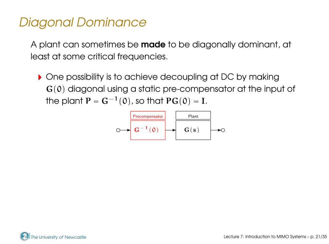
A plant can sometimes be made to be diagonally dominant, at
least at some critical frequencies.
One possibility is to achieve decoupling at DC by making
G(0) diagonal using a static pre-compensator at the input of
the plant P = G−1(0), so that PG(0) = I.
c c
Precompensator Plant
--- G(s)G−1(0)
Lecture 7: Introduction to MIMO Systems – p. 21/35

The University of Newcastle
Diagonal Dominance
A plant can sometimes be made to be diagonally dominant, at
least at some critical frequencies.
One possibility is to achieve decoupling at DC by making
G(0) diagonal using a static pre-compensator at the input of
the plant P = G−1(0), so that PG(0) = I.
c c
Precompensator Plant
--- G(s)G−1(0)
For the four tank example, the pre-compensator is
P =
3.7γ 3.7(1 − γ)
4.7(1 − γ) 4.7γ
−1
=1
3.7 × 4.7(2γ − 1)
4.7γ 3.7(γ − 1)
4.7(γ − 1) 3.7γ
Lecture 7: Introduction to MIMO Systems – p. 21/35
The University of Newcastle
Diagonal Dominance
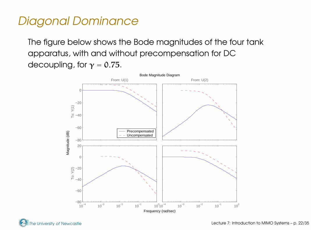
The figure below shows the Bode magnitudes of the four tank
apparatus, with and without precompensation for DC
decoupling, for γ = 0.75.Bode Magnitude Diagram
Frequency (rad/sec)
Mag
nitu
de (
dB)
−80
−60
−40
−20
0
From: U(1)
To:
Y(1
)
PrecompensatedUncompensated
10−4
10−3
10−2
10−1
100
−80
−60
−40
−20
0
20
To:
Y(2
)
From: U(2)
10−4
10−3
10−2
10−1
100
Lecture 7: Introduction to MIMO Systems – p. 22/35
The University of Newcastle
Decentralised Control and the RGA
If a plant transfer matrix is diagonally dominant, it may be
possible to design a good controller by considering each
input-output pair as a separate loop. This approach is sometimes
called decentralised control.
An important issue in decentralised control design is the
appropriate selection of input-output pairs (Note that they
will not in general be arranged so that G(s) is diagonal).
Lecture 7: Introduction to MIMO Systems – p. 23/35
The University of Newcastle
Decentralised Control and the RGA
If a plant transfer matrix is diagonally dominant, it may be
possible to design a good controller by considering each
input-output pair as a separate loop. This approach is sometimes
called decentralised control.
An important issue in decentralised control design is the
appropriate selection of input-output pairs (Note that they
will not in general be arranged so that G(s) is diagonal).
One way of choosing the pairing is via the relative gain array
(RGA) Λ, given by
Λ = G(0) . ∗ G−1(0)T
where .∗ denotes element-wise multiplication.
Lecture 7: Introduction to MIMO Systems – p. 23/35

The University of Newcastle
Decentralised Control and the RGA
If a plant transfer matrix is diagonally dominant, it may be
possible to design a good controller by considering each
input-output pair as a separate loop. This approach is sometimes
called decentralised control.
An important issue in decentralised control design is the
appropriate selection of input-output pairs (Note that they
will not in general be arranged so that G(s) is diagonal).
One way of choosing the pairing is via the relative gain array
(RGA) Λ, given by
Λ = G(0) . ∗ G−1(0)T
where .∗ denotes element-wise multiplication.
Each row and column in the RGA always sums to 1, and the
values are independent of units (e.g., A or mA, m or mm).
Lecture 7: Introduction to MIMO Systems – p. 23/35
The University of Newcastle
Decentralised Control and the RGA
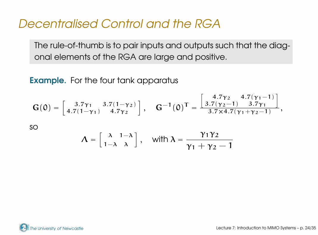
The rule-of-thumb is to pair inputs and outputs such that the diag-
onal elements of the RGA are large and positive.
Lecture 7: Introduction to MIMO Systems – p. 24/35
The University of Newcastle
Decentralised Control and the RGA
The rule-of-thumb is to pair inputs and outputs such that the diag-
onal elements of the RGA are large and positive.
Example. For the four tank apparatus
G(0) =[
3.7γ1 3.7(1−γ2)
4.7(1−γ1) 4.7γ2
]
, G−1(0)T =
[
4.7γ2 4.7(γ1−1)
3.7(γ2−1) 3.7γ1
]
3.7×4.7(γ1+γ2−1),
so
Λ =[
λ 1−λ
1−λ λ
]
, with λ =γ1γ2
γ1 + γ2 − 1
Lecture 7: Introduction to MIMO Systems – p. 24/35

The University of Newcastle
Decentralised Control and the RGA
The rule-of-thumb is to pair inputs and outputs such that the diag-
onal elements of the RGA are large and positive.
Example. For the four tank apparatus
G(0) =[
3.7γ1 3.7(1−γ2)
4.7(1−γ1) 4.7γ2
]
, G−1(0)T =
[
4.7γ2 4.7(γ1−1)
3.7(γ2−1) 3.7γ1
]
3.7×4.7(γ1+γ2−1),
so
Λ =[
λ 1−λ
1−λ λ
]
, with λ =γ1γ2
γ1 + γ2 − 1
If γ1 = γ2 = γ, and γ = 1, the RGA rule suggests the pairing
(u1, y1) and (u2, y2). On the other hand, if γ = 0, the pairing
suggested is the opposite, (u1, y2), (u2, y1).
Lecture 7: Introduction to MIMO Systems – p. 24/35

The University of Newcastle
MIMO Sensitivity Functions
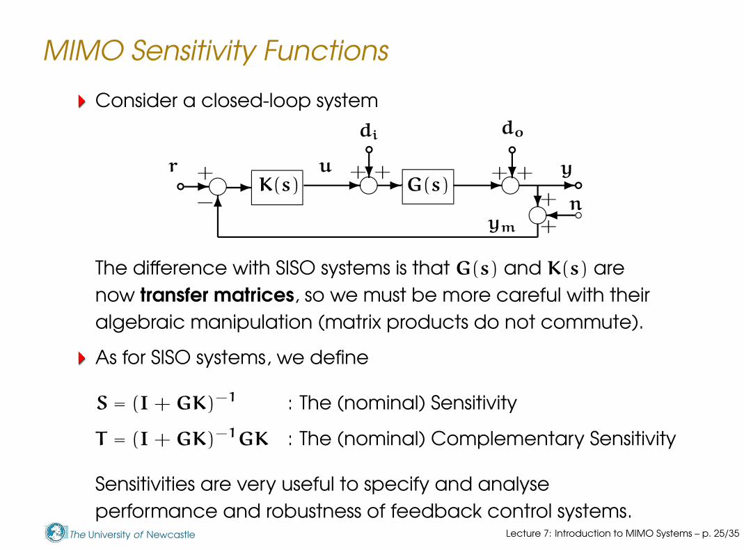
Consider a closed-loop system
h h h
h
- - - ?
6 ¾
?+
+
+b
b
bb
b ..- - -?
r
do
G(s)+ + y+
−K(s)
+u
di
nym
The difference with SISO systems is that G(s) and K(s) are
now transfer matrices, so we must be more careful with their
algebraic manipulation (matrix products do not commute).
Lecture 7: Introduction to MIMO Systems – p. 25/35
The University of Newcastle
MIMO Sensitivity Functions
Consider a closed-loop system
h h h
h
- - - ?
6 ¾
?+
+
+b
b
bb
b ..- - -?
r
do
G(s)+ + y+
−K(s)
+u
di
nym
The difference with SISO systems is that G(s) and K(s) are
now transfer matrices, so we must be more careful with their
algebraic manipulation (matrix products do not commute).
As for SISO systems, we define
S = (I + GK)−1 : The (nominal) Sensitivity
T = (I + GK)−1GK : The (nominal) Complementary Sensitivity
Sensitivities are very useful to specify and analyse
performance and robustness of feedback control systems.Lecture 7: Introduction to MIMO Systems – p. 25/35
The University of Newcastle
Performance and Robustness
Many of the measures of performance and robustness of
MIMO systems can be expressed in terms of the gains of the
sensitivities.
Lecture 7: Introduction to MIMO Systems – p. 26/35
The University of Newcastle
Performance and Robustness
Many of the measures of performance and robustness of
MIMO systems can be expressed in terms of the gains of the
sensitivities.
However, it is certainly difficult to specify desired
performance for n × n scalar transfer functions, if say we
have a n-input n-output plant.
We often obtain more useful results if we consider the
principal gains rather than the gains of each element in the
transfer function matrix.
The principal gains are the singular values of the complex
transfer function matrix.
σi(jω) =
√
eig [G(jω)GH(jω)]
where (.)H denotes the conjugate transpose.
Lecture 7: Introduction to MIMO Systems – p. 26/35
The University of Newcastle
Performance and Robustness
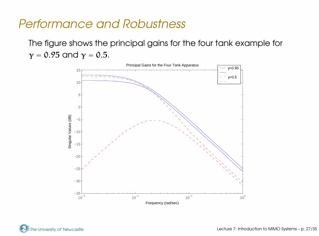
The figure shows the principal gains for the four tank example for
γ = 0.95 and γ = 0.5.Principal Gains for the Four Tank Apparatus
Frequency (rad/sec)
Sin
gula
r V
alue
s (d
B)
10−3
10−2
10−1
100
−35
−30
−25
−20
−15
−10
−5
0
5
10
15γ=0.95 γ=0.5
Lecture 7: Introduction to MIMO Systems – p. 27/35
The University of Newcastle
Performance and Robustness
If we have a result for a SISO (single-input single-output) system
requiring an upper bound on a certain gain, then it is likely to
generalise to a MIMO (multivariable) system as requiring an
upper bound on the corresponding maximum principal gain.
σmax(jω) = maxi
σi(jω)
For the SISO case good tracking in some bandwidth 0 ≤ ω ≤ B
requires T ≈ 1. This in turn requires S ≈ 0 in the corresponding
bandwidth.
For the MIMO case this becomes the requirement σmax(S) ≈ 0
within that range of frequencies. This is equivalent to the
requirement that
T ≈ I, for ω ∈ [0, B]
In MATLAB the principal gains can be computed with the
function sigma.Lecture 7: Introduction to MIMO Systems – p. 28/35

The University of Newcastle
MIMO Control Design
The generalisation of IMC design methodology for square MIMO
systems is straightforward. The parameterisation of all controllers
that yield a stable closed-loop system for a stable plant with
nominal model G0(s) is given by
K(s) = [I − Q(s)G0(s)]−1Q(s) = Q(s)[I − G0(s)Q(s)]−1,
where Q(s) is any stable proper transfer matrix.
Lecture 7: Introduction to MIMO Systems – p. 29/35

The University of Newcastle
MIMO Control Design
The generalisation of IMC design methodology for square MIMO
systems is straightforward. The parameterisation of all controllers
that yield a stable closed-loop system for a stable plant with
nominal model G0(s) is given by
K(s) = [I − Q(s)G0(s)]−1Q(s) = Q(s)[I − G0(s)Q(s)]−1,
where Q(s) is any stable proper transfer matrix.
Example. Consider again the 2-input, 2-output plant
represented by
G(s) =
4(s+1)(s+2)
−1(s+1)
2(s+1)
−12(s+1)(s+2)
Lecture 7: Introduction to MIMO Systems – p. 29/35
The University of Newcastle
MIMO Control Design
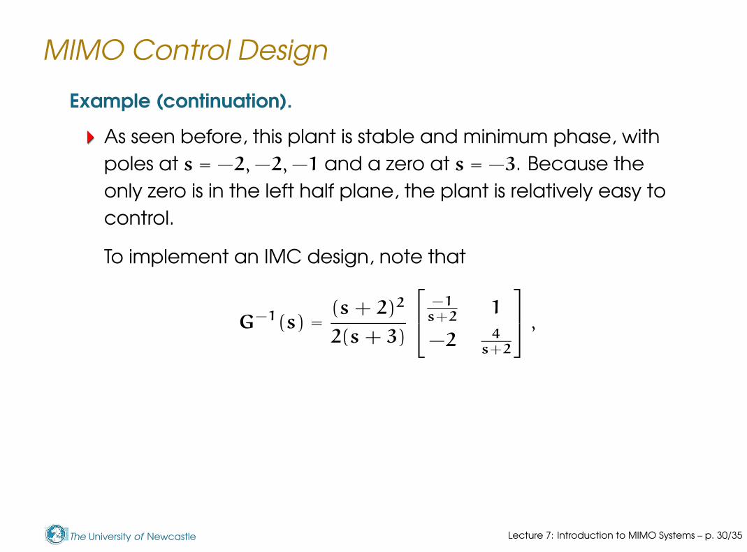
Example (continuation).
As seen before, this plant is stable and minimum phase, with
poles at s = −2, −2, −1 and a zero at s = −3. Because the
only zero is in the left half plane, the plant is relatively easy to
control.
To implement an IMC design, note that
G−1(s) =(s + 2)2
2(s + 3)
−1s+2
1
−2 4s+2
,
Lecture 7: Introduction to MIMO Systems – p. 30/35
The University of Newcastle
MIMO Control Design
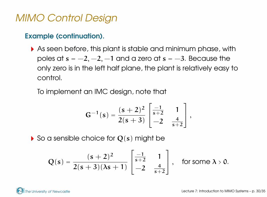
Example (continuation).
As seen before, this plant is stable and minimum phase, with
poles at s = −2, −2, −1 and a zero at s = −3. Because the
only zero is in the left half plane, the plant is relatively easy to
control.
To implement an IMC design, note that
G−1(s) =(s + 2)2
2(s + 3)
−1s+2
1
−2 4s+2
,
So a sensible choice for Q(s) might be
Q(s) =(s + 2)2
2(s + 3)(λs + 1)
−1s+2
1
−2 4s+2
, for some λ > 0.
Lecture 7: Introduction to MIMO Systems – p. 30/35

The University of Newcastle
MIMO Control Design
Example (continuation). We implement in Simulink this IMC
design for λ = 1, including step references and input
disturbances.Disturbances
References
Y
U
Step3
Step2
Step1
Step
G0
LTI System2
G
LTI System1
Q
LTI System
2
2
2
2
2
2
2
22
2
2
2
2
22
Lecture 7: Introduction to MIMO Systems – p. 31/35
The University of Newcastle
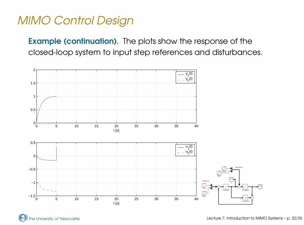
MIMO Control Design
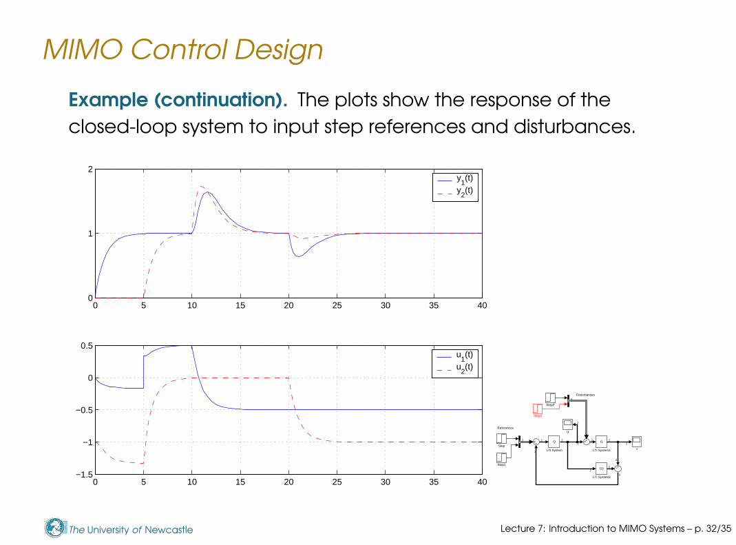
Example (continuation). The plots show the response of the
closed-loop system to input step references and disturbances.
0 5 10 15 20 25 30 35 40−1.5
−1
−0.5
0
0.5
t [s]
u1(t)
u2(t)
0 5 10 15 20 25 30 35 400
0.5
1
1.5
2
t [s]
y1(t)
y2(t)
Disturbances
References
Y
U
Step3
Step2
Step1
Step
G0
LTI System2
G
LTI System1
Q
LTI System
2
2
2
2
2
2
2
22
2
2
2
2
22
Lecture 7: Introduction to MIMO Systems – p. 32/35
The University of Newcastle
MIMO Control Design
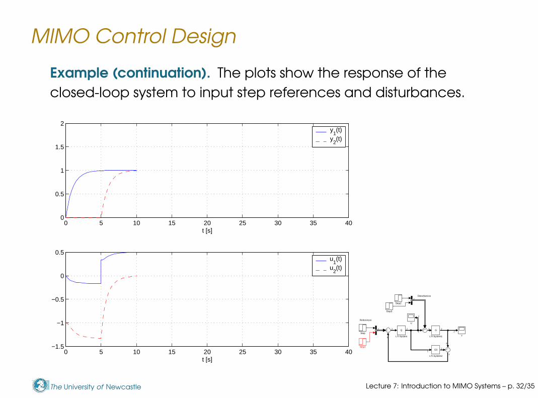
Example (continuation). The plots show the response of the
closed-loop system to input step references and disturbances.
0 5 10 15 20 25 30 35 40−1.5
−1
−0.5
0
0.5
t [s]
u1(t)
u2(t)
0 5 10 15 20 25 30 35 400
0.5
1
1.5
2
t [s]
y1(t)
y2(t)
Disturbances
References
Y
U
Step3
Step2
Step1
Step
G0
LTI System2
G
LTI System1
Q
LTI System
2
2
2
2
2
2
2
22
2
2
2
2
22
Lecture 7: Introduction to MIMO Systems – p. 32/35

The University of Newcastle
MIMO Control Design
Example (continuation). The plots show the response of the
closed-loop system to input step references and disturbances.
0 5 10 15 20 25 30 35 40−1.5
−1
−0.5
0
0.5
t [s]
u1(t)
u2(t)
0 5 10 15 20 25 30 35 400
0.5
1
1.5
2
t [s]
y1(t)
y2(t)
Disturbances
References
Y
U
Step3
Step2
Step1
Step
G0
LTI System2
G
LTI System1
Q
LTI System
2
2
2
2
2
2
2
22
2
2
2
2
22
Lecture 7: Introduction to MIMO Systems – p. 32/35
The University of Newcastle
MIMO Control Design
Example (continuation). The plots show the response of the
closed-loop system to input step references and disturbances.
0 5 10 15 20 25 30 35 40−1.5
−1
−0.5
0
0.5u
1(t)
u2(t)
0 5 10 15 20 25 30 35 400
1
2y
1(t)
y2(t)
Disturbances
References
Y
U
Step3
Step2
Step1
Step
G0
LTI System2
G
LTI System1
Q
LTI System
2
2
2
2
2
2
2
22
2
2
2
2
22
Lecture 7: Introduction to MIMO Systems – p. 32/35
The University of Newcastle
Difficulties of MIMO IMC Design
However, in general the choice of a suitable matrix Q(s) for a
MIMO IMC design becomes much more complicated than in
SISO systems.
In particular, the key attributes in the synthesis of Q(s)
relative-degree (i.e., zeros at infinity)
inverse stability (i.e., NMP zeros)
exhibit significant complexity in MIMO systems and require
additional tools to account for directionality issues.
Lecture 7: Introduction to MIMO Systems – p. 33/35
The University of Newcastle
Difficulties of MIMO IMC Design
However, in general the choice of a suitable matrix Q(s) for a
MIMO IMC design becomes much more complicated than in
SISO systems.
In particular, the key attributes in the synthesis of Q(s)
relative-degree (i.e., zeros at infinity)
inverse stability (i.e., NMP zeros)
exhibit significant complexity in MIMO systems and require
additional tools to account for directionality issues.
In addition, the computations associated with IMC design
can get very arduous for other than low dimension, square
MIMO systems.
How can we deal with possibly difficult, nonsquare, large
scale MIMO systems?
Use state space control design!
Lecture 7: Introduction to MIMO Systems – p. 33/35
The University of Newcastle
Summary
SISO transfer functions generalise to MIMO as transfer matrix
functions, with the associated (although more subtle)
concepts of poles and zeros. Transfer matrix manipulations
are more complex, since matrix products do not commute.
Lecture 7: Introduction to MIMO Systems – p. 34/35

The University of Newcastle
Summary
SISO transfer functions generalise to MIMO as transfer matrix
functions, with the associated (although more subtle)
concepts of poles and zeros. Transfer matrix manipulations
are more complex, since matrix products do not commute.
Many control problems require multiple inputs to be
manipulated simultaneously in an orchestrated manner. A
key difficulty in achieving an appropriate orchestration of the
inputs is the multivariable directionality, or coupling.
Lecture 7: Introduction to MIMO Systems – p. 34/35
The University of Newcastle
Summary
SISO transfer functions generalise to MIMO as transfer matrix
functions, with the associated (although more subtle)
concepts of poles and zeros. Transfer matrix manipulations
are more complex, since matrix products do not commute.
Many control problems require multiple inputs to be
manipulated simultaneously in an orchestrated manner. A
key difficulty in achieving an appropriate orchestration of the
inputs is the multivariable directionality, or coupling.
Decentralised control might be an option when the plant is
diagonally dominant. A practical rule to pair inputs and
outputs is based on the Relative Gain Array.
Lecture 7: Introduction to MIMO Systems – p. 34/35
The University of Newcastle
Summary
The concepts of stability, sensitivity functions, performance
and robustness, generalise directly to MIMO systems.
Lecture 7: Introduction to MIMO Systems – p. 35/35
The University of Newcastle
Summary
The concepts of stability, sensitivity functions, performance
and robustness, generalise directly to MIMO systems.
IMC design for MIMO systems is essentially the same as for
SISO systems. Yet, the synthesis process is more subtle, and
the required computations may get much more involved.
We will come back to MIMO systems with State Space
System Theory and Control Design.
Lecture 7: Introduction to MIMO Systems – p. 35/35