Lecture 7: Decision Trees - GitHub Pages
87
Lecture 7: Decision Trees Instructor: Saravanan Thirumuruganathan CSE 5334 Saravanan Thirumuruganathan
Transcript of Lecture 7: Decision Trees - GitHub Pages

Lecture 7: Decision Trees
Instructor: Saravanan Thirumuruganathan
CSE 5334 Saravanan Thirumuruganathan

Outline
1 Geometric Perspective of Classification
2 Decision Trees
CSE 5334 Saravanan Thirumuruganathan

Geometric Perspective ofClassification
CSE 5334 Saravanan Thirumuruganathan

Perspective of Classification
Algorithmic
Geometric
Probabilistic
. . .
CSE 5334 Saravanan Thirumuruganathan

Geometric Perspective of Classification
Gives some intuition for model selection
Understand the distribution of data
Understand the expressiveness and limitations of variousclassifiers
CSE 5334 Saravanan Thirumuruganathan

Feature Space1
Feature Vector: d-dimensional vector of features describingthe object
Feature Space: The vector space associated with featurevectors
1DMA BookCSE 5334 Saravanan Thirumuruganathan

Feature Space in Classification
CSE 5334 Saravanan Thirumuruganathan

Geometric Perspective of Classification
Decision Region: A partition of feature space such that allfeature vectors in it are assigned to same class.
Decision Boundary: Boundaries between neighboringdecision regions
CSE 5334 Saravanan Thirumuruganathan

Geometric Perspective of Classification
Objective of a classifier is to approximate the “real” decisionboundary as much as possible
Most classification algorithm has specific expressiveness andlimitations
If they align, then classifier does a good approximation
CSE 5334 Saravanan Thirumuruganathan

Linear Decision Boundary
CSE 5334 Saravanan Thirumuruganathan

Piecewise Linear Decision Boundary2
2ISLR BookCSE 5334 Saravanan Thirumuruganathan

Quadratic Decision Boundary3
3Figshare.comCSE 5334 Saravanan Thirumuruganathan

Non-linear Decision Boundary4
4ISLR BookCSE 5334 Saravanan Thirumuruganathan

Complex Decision Boundary5
5ISLR Book CSE 5334 Saravanan Thirumuruganathan
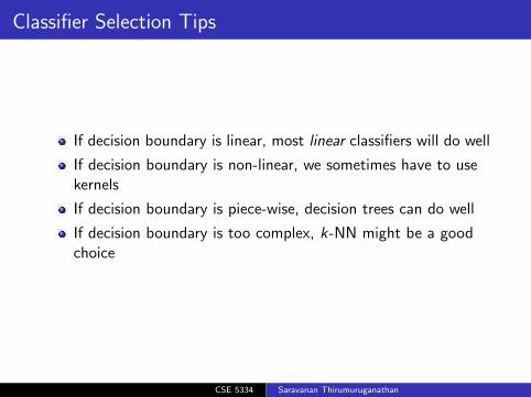
Classifier Selection Tips
If decision boundary is linear, most linear classifiers will do well
If decision boundary is non-linear, we sometimes have to usekernels
If decision boundary is piece-wise, decision trees can do well
If decision boundary is too complex, k-NN might be a goodchoice
CSE 5334 Saravanan Thirumuruganathan

k-NN Decision Boundary6
Asymptotically Consistent: With infinite training data andlarge enough k , k-NN approaches the best possible classifier(Bayes Optimal)
With infinite training data and large enough k , k-NN couldapproximate most possible decision boundaries
6ISLR BookCSE 5334 Saravanan Thirumuruganathan

Decision Trees
CSE 5334 Saravanan Thirumuruganathan

Strategies for Classifiers
Parametric Models: Makes some assumption about datadistribution such as density and often use explicit probabilitymodels
Non-parametric Models: No prior assumption of data anddetermine decision boundaries directly.
k-NNDecision tree
CSE 5334 Saravanan Thirumuruganathan

Tree7
7http:
//statweb.stanford.edu/~lpekelis/talks/13_datafest_cart_talk.pdfCSE 5334 Saravanan Thirumuruganathan

Binary Decision Tree8
8http:
//statweb.stanford.edu/~lpekelis/talks/13_datafest_cart_talk.pdfCSE 5334 Saravanan Thirumuruganathan

20 Question Intuition9
9http://www.idiap.ch/~fleuret/files/EE613/EE613-slides-6.pdf
CSE 5334 Saravanan Thirumuruganathan

Decision Tree for Selfie Stick10
10The Oatmeal ComicsCSE 5334 Saravanan Thirumuruganathan

Decision Trees and Rules11
11http://artint.info/slides/ch07/lect3.pdf
CSE 5334 Saravanan Thirumuruganathan

Decision Trees and Rules12
long → skips
short ∧ new → reads
short ∧ follow Up ∧ known →reads
short ∧ follow Up ∧ unknown →skips
12http://artint.info/slides/ch07/lect3.pdf
CSE 5334 Saravanan Thirumuruganathan

Building Decision Trees Intuition13
Horsepower Weight Mileage95 low low
90 low low
70 low high
86 low high
76 high low
88 high low
Table: Car Mileage Prediction from 1971
13http://spark-summit.org/wp-content/uploads/2014/07/
Scalable-Distributed-Decision-Trees-in-Spark-Made-Das-Sparks-Talwalkar.
CSE 5334 Saravanan Thirumuruganathan

Building Decision Trees Intuition
Horsepower Weight Mileage95 low low
90 low low
70 low high
86 low high
76 high low
88 high low
Table: Car Mileage Prediction from 1971
CSE 5334 Saravanan Thirumuruganathan

Building Decision Trees Intuition
CSE 5334 Saravanan Thirumuruganathan

Building Decision Trees Intuition
Horsepower Weight Mileage95 low low
90 low low
70 low high
86 low high
Table: Car Mileage Prediction from 1971
CSE 5334 Saravanan Thirumuruganathan

Building Decision Trees Intuition
CSE 5334 Saravanan Thirumuruganathan

Building Decision Trees Intuition
CSE 5334 Saravanan Thirumuruganathan
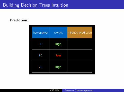
Building Decision Trees Intuition
Prediction:
CSE 5334 Saravanan Thirumuruganathan

Building Decision Trees Intuition
Prediction:
CSE 5334 Saravanan Thirumuruganathan

Learning Decision Trees
CSE 5334 Saravanan Thirumuruganathan

Decision Trees
Defined by a hierarchy of rules (in form of a tree)
Rules form the internal nodes of the tree (topmost internalnode = root)
Each rule (internal node) tests the value of some property thedata
Leaf nodes make the prediction
CSE 5334 Saravanan Thirumuruganathan

Decision Tree Learning
Objective:
Use the training data to construct a good decision tree
Use the constructed Decision tree to predict labels for testinputs
CSE 5334 Saravanan Thirumuruganathan

Decision Tree Learning
Identifying the region (blue or green) a point lies in
A classification problem (blue vs green)Each input has 2 features: co-ordinates {x1, x2} in the 2Dplane
Once learned, the decision tree can be used to predict theregion (blue/green) of a new test point
CSE 5334 Saravanan Thirumuruganathan

Decision Tree Learning
CSE 5334 Saravanan Thirumuruganathan

Expressiveness of Decision Trees
CSE 5334 Saravanan Thirumuruganathan

Expressiveness of Decision Trees
Decision tree divides feature space into axis-parallelrectangles
Each rectangle is labelled with one of the C classes
Any partition of feature space by recursive binary splitting canbe simulated by Decision Trees
CSE 5334 Saravanan Thirumuruganathan

Expressiveness of Decision Trees
Feature space on left can be simulated by Decision tree but notthe one on right.
CSE 5334 Saravanan Thirumuruganathan

Expressiveness of Decision Trees
Feature space on left can be simulated by Decision tree but notthe one on right.
CSE 5334 Saravanan Thirumuruganathan

Expressiveness of Decision Tree
Can express any logicalfunction on input attributes
Can express any booleanfunction
For boolean functions,path to leaf gives truthtable row
Could require exponentiallymany nodes
cyl = 3 ∨ (cyl =4∧(maker = asia∨maker =europe)) ∨ . . .
CSE 5334 Saravanan Thirumuruganathan

Hypothesis Space
Exponential search space wrt set of attributes
If there are d boolean attributes, then the search space has
22d
trees
If d = 6, then it is approximately18, 446, 744, 073, 709, 551, 616 (or approximately 1.8× 10¹⁸)If there are d boolean attributes, each truth table has 2d rowsHence there must be 22d truth tables that can take all possiblevariationsAlternate argument: the number of trees is same as
number of bolean functions with d variables= number of distinct truth tables with 2d rows = 22
d
NP-Complete to find optimal decision tree
Idea: Use greedy approach to find a locally optimal tree
CSE 5334 Saravanan Thirumuruganathan

Decision Tree Learning Algorithms
1966: Hunt and colleagues from Psychology developed firstknown algorithm for human concept learning
1977: Breiman, Friedman and others from Statisticsdeveloped CART
1979: Quinlan developed proto-ID3
1986: Quinlan published ID3 paper
1993: Quinlan’s updated algorithm C4.5
1980’s and 90’s: Improvements for handling noise, continuousattributes, missing data, non-axis parallel DTs, betterheuristics for pruning, overfitting, combining DTs
CSE 5334 Saravanan Thirumuruganathan

Decision Tree Learning Algorithms
Main Loop:
1 Let A be the “best” decision attribute for next node
2 Assign A as decision attribute for node
3 For each value of A, create a new descendent of node
4 Sort training examples to leaf nodes
5 If training examples are perfectly classified, then STOP elseiterate over leaf nodes
CSE 5334 Saravanan Thirumuruganathan

Recursive Algorithm for Learning Decision Trees
CSE 5334 Saravanan Thirumuruganathan

Decision Tree Learning
Greedy Approach: Build tree, top-down by choosing oneattribute at a time
Choices are locally optimal and may or may not be globallyoptimal
Major issues
Selecting the next attributeGiven an attribute, how to specify the split conditionDetermining termination condition
CSE 5334 Saravanan Thirumuruganathan

Termination Condition
Stop expanding a node further when:
It consist of examples all having the same label
Or we run out of features to test!
CSE 5334 Saravanan Thirumuruganathan
Termination Condition
Stop expanding a node further when:
It consist of examples all having the same label
Or we run out of features to test!
CSE 5334 Saravanan Thirumuruganathan

How to Specify Test Condition?
Depends on attribute types
NominalOrdinalContinuous
Depends on number of ways to split
2-way splitMulti-way split
CSE 5334 Saravanan Thirumuruganathan

Splitting based on Nominal Attributes
CSE 5334 Saravanan Thirumuruganathan

Splitting based on Ordinal Attributes
CSE 5334 Saravanan Thirumuruganathan
Splitting based on Continuous Attributes
How to split continuous attributes such as Age, Income etc
Discretization to form an ordinal categorical attribute
Static: discretize once at the beginningDynamic: find ranges by equal interval bucketing, equalfrequency bucketing, percentiles, clustering etc
Binary Decision: (A < v)or(A ≥ v)
Consider all possible split and find the best cutOften, computationally intensive
CSE 5334 Saravanan Thirumuruganathan

Splitting based on Continuous Attributes
CSE 5334 Saravanan Thirumuruganathan

Choosing the next Attribute - I
CSE 5334 Saravanan Thirumuruganathan

Choosing the next Attribute - II14
14http://www.cedar.buffalo.edu/~srihari/CSE574/Chap16/Chap16.
1-InformationGain.pdf
CSE 5334 Saravanan Thirumuruganathan

Choosing the next Attribute - III
CSE 5334 Saravanan Thirumuruganathan

Choosing an Attribute
Good Attribute
for one value we get all instances as positivefor other value we get all instances as negative
Bad Attribute
it provides no discriminationattribute is immaterial to the decisionfor each value we have same number of positive and negativeinstances
CSE 5334 Saravanan Thirumuruganathan

How to Find the Best Split?
CSE 5334 Saravanan Thirumuruganathan

Measures of Node Impurity
Gini Index
Entropy
Misclassification Error
CSE 5334 Saravanan Thirumuruganathan

Gini Index
An important measure of statistical dispersion
Used in Economics to measure income inequality in countries
Proposed by Corrado Gini
CSE 5334 Saravanan Thirumuruganathan

Gini Index
CSE 5334 Saravanan Thirumuruganathan

Gini Index
CSE 5334 Saravanan Thirumuruganathan

Splitting Based on Gini
Used in CART, SLIQ, SPRINT
When a node p is split into k partitions (children), the qualityof split is computed as,
Ginisplit =k∑
i=1
ninGini(i)
ni = number of records at child in = number of records at node p
CSE 5334 Saravanan Thirumuruganathan

Gini Index for Binary Attributes
CSE 5334 Saravanan Thirumuruganathan

Gini Index for Categorical Attributes
CSE 5334 Saravanan Thirumuruganathan

Entropy and Information Gain
You are watching a set of independent random samples of arandom variable X
Suppose the probabilities are equal:P(X = A) = P(X = B) = P(X = C ) = P(X = D) = 1
4
Suppose you see a text like BAAC
You want to transmit this information in a binarycommunication channel
How many bits will you need to transmit this information?
Simple idea: Represent each character via 2 bits:A = 00,B = 01,C = 10,D = 11
So, BAAC becomes 01000010
Communication Complexity: 2 on average bits per symbol
CSE 5334 Saravanan Thirumuruganathan

Entropy and Information Gain
Suppose you knew probabilities are unequal:P(X = A) = 1
2 ,P(X = B) = 14 ,P(X = C ) = P(X = D) = 1
8
It is now possible to send information 1.75 bits on average persymbol
Choose a frequency based code!
A = 0,B = 10,C = 110,D = 111
BAAC becomes 1000110
Requires only 7 bits for transmitting BAAC
CSE 5334 Saravanan Thirumuruganathan

Entropy
CSE 5334 Saravanan Thirumuruganathan

Entropy
CSE 5334 Saravanan Thirumuruganathan

Entropy
CSE 5334 Saravanan Thirumuruganathan

Entropy
CSE 5334 Saravanan Thirumuruganathan

Splitting based on Classification Error
Classification error at node t is
Error(t) = 1−maxiP(i |t)
Measures misclassification error made by a node.
Minimum (0.0) when all records belong to one class, implyingmost interesting informationMaximum (1− 1
nc) when records are equally distributed among
all classes, implying least interesting information
CSE 5334 Saravanan Thirumuruganathan

Classification Error
CSE 5334 Saravanan Thirumuruganathan

Comparison among Splitting Criteria
CSE 5334 Saravanan Thirumuruganathan

Splitting Criteria
Gini Index (CART, SLIQ, SPRINT):
select attribute that minimize impurity of a split
Information Gain (ID3, C4.5)
select attribute with largest information gain
Normalized Gain ratio (C4.5)
normalize different domains of attributes
Distance normalized measures (Lopez de Mantaras)
define a distance metric between partitions of the datachose the one closest to the perfect partition
χ2 contingency table statistics (CHAID)
measures correlation between each attribute and the class labelselect attribute with maximal correlation
CSE 5334 Saravanan Thirumuruganathan

Overfitting in Decision Trees
Decision trees will always overfit in the absence of label noise
Simple strategies for fixing:
Fixed depthFixed number of leavesGrow the tree till the gain is above some thresholdPost pruning
CSE 5334 Saravanan Thirumuruganathan

Trees vs Linear Models
CSE 5334 Saravanan Thirumuruganathan

Advantages and Disadvantages
Very easy to explain to people.
Some people believe that decision trees more closely mirrorhuman decision-making
Trees can be displayed graphically, and are easily interpretedeven by a non-expert (especially if they are small)
Trees can easily handle qualitative predictors without the needto create dummy variables.
Inexpensive to construct
Extremely fast at classifying new data
Unfortunately, trees generally do not have the same level ofpredictive accuracy as other classifiers
CSE 5334 Saravanan Thirumuruganathan

Summary
Major Concepts:Geometric interpretation of Classification
Decision trees
CSE 5334 Saravanan Thirumuruganathan

Slide Material References
Slides from ISLR book
Slides by Piyush Rai
Slides for Chapter 4 from “Introduction to Data Mining” bookby Tan, Steinbach, Kumar
Slides from Andrew Moore, CMU
See also the footnotes
CSE 5334 Saravanan Thirumuruganathan