Lecture 6:

• Maximum Likelihood • Neyman-Pearson Lemma • Wilk’s Theorem • Extended Likelihood

We wish to express the likelihood for a given set of data to have resulted from a particular model of probability distributions:

for independent events

Maximum Likelihood

More likely data sets for H(q) will have a higher combined probability (i.e. likelihood)

likelihood data set

conditional probability

assuming a particular hypothesis defined by a set of parameters q

L = P (D |H(q))

more practical to compute

log L =n

∑i=1

log [P (xi |H(q))]

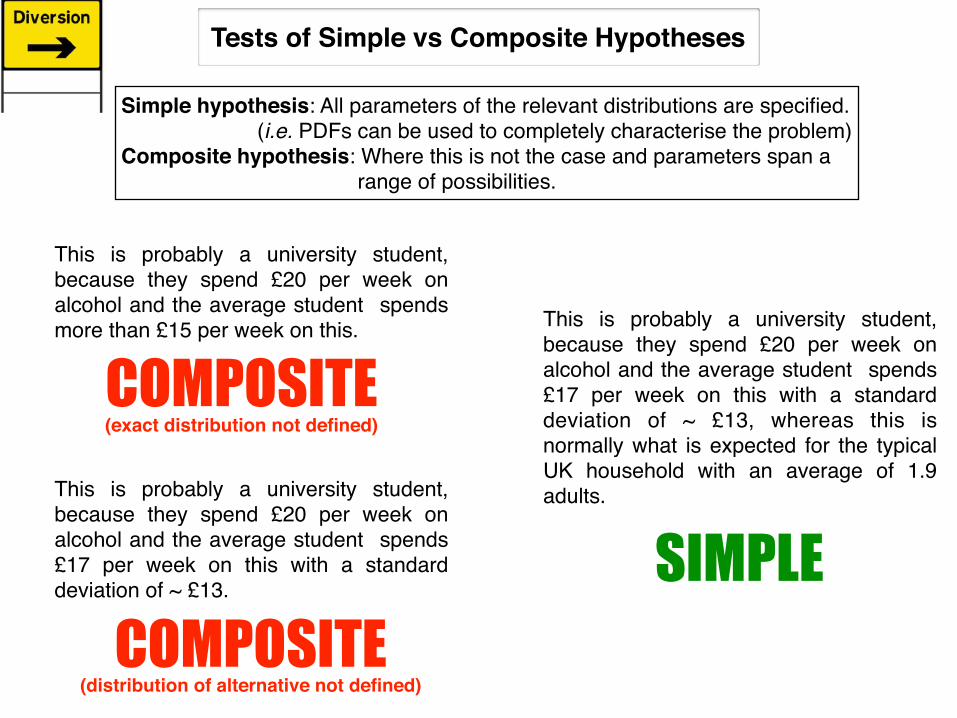
Simple hypothesis: All parameters of the relevant distributions are specified. (i.e. PDFs can be used to completely characterise the problem)Composite hypothesis: Where this is not the case and parameters span a range of possibilities.

This is probably a university student, because they spend £20 per week on alcohol and the average student spends more than £15 per week on this.

This is probably a university student, because they spend £20 per week on alcohol and the average student spends £17 per week on this with a standard deviation of ~ £13.

This is probably a university student, because they spend £20 per week on alcohol and the average student spends £17 per week on this with a standard deviation of ~ £13, whereas this is normally what is expected for the typical UK household with an average of 1.9 adults.

SIMPLE

COMPOSITE(exact distribution not defined)

COMPOSITE(distribution of alternative not defined)

Tests of Simple vs Composite Hypotheses

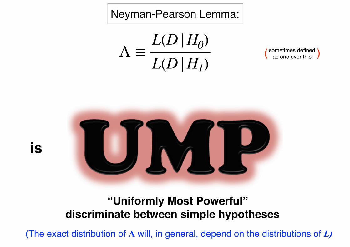
Λ ≡ L(D |H0)L(D |H1)

Neyman-Pearson Lemma:

“Uniformly Most Powerful”discriminate between simple hypotheses

is

(The exact distribution of Λ will, in general, depend on the distributions of L)

sometimes defined as one over this( )

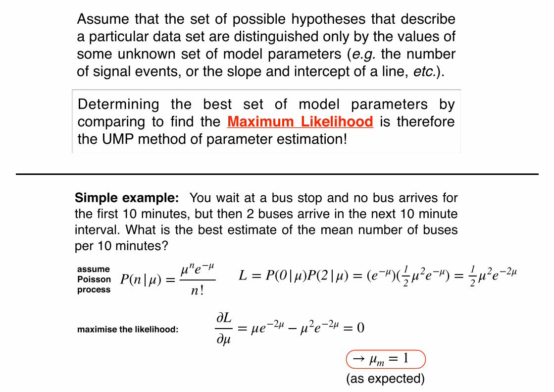
Assume that the set of possible hypotheses that describe a particular data set are distinguished only by the values of some unknown set of model parameters (e.g. the number of signal events, or the slope and intercept of a line, etc.).

Determining the best set of model parameters by comparing to find the Maximum Likelihood is therefore the UMP method of parameter estimation!

Simple example: You wait at a bus stop and no bus arrives for the first 10 minutes, but then 2 buses arrive in the next 10 minute interval. What is the best estimate of the mean number of buses per 10 minutes?

P(n |μ) = μne−μ

n!assume Poisson process

L = P(0 |μ)P(2 |μ) = (e−μ)( 12 μ2e−μ) = 1

2 μ2e−2μ

→ μm = 1(as expected)

maximise the likelihood:∂L∂μ

= μe−2μ − μ2e−2μ = 0

constant

Thus, maximising L = maximising logL = minimising -2logL is equivalent to the Method of Least Squares in this limit !!

=NX

i=1

log1p2⇡�i

�NX

i=1

(xi � µi)2

2�2i

Consider the case where uncertainties on data points are normally distributed. Assume that the mean values and variances, µi and σi, are predicted at each data point by some model. Then we have:

logL =NX

i=1

log

1p2⇡�i

exp

✓� (xi � µi)2

2�2i

◆�log L

thus, �2 logL = �2NX

i=1

log1p2⇡�i

+NX

i=1

(xi � µi)2

�2i

log L

looks like χ2

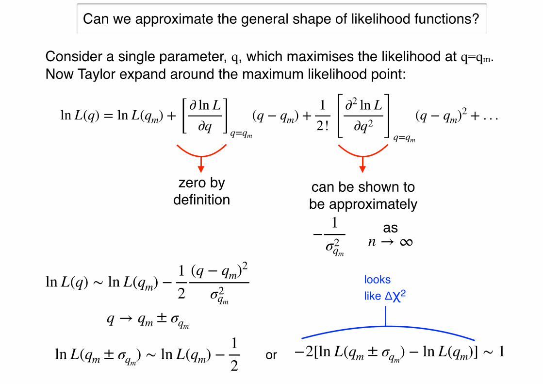
Consider a single parameter, q, which maximises the likelihood at q=qm. Now Taylor expand around the maximum likelihood point:

ln L(q) = ln L(qm) + [ ∂ ln L∂q ]

q=qm

(q − qm) + 12! [ ∂2 ln L

∂q2 ]q=qm

(q − qm)2 + . . .

zero by definition

can be shown to be approximately

− 1σ2qm

asn → ∞

ln L(q) ∼ ln L(qm) − 12

(q − qm)2

σ2qm

ln L(qm ± σqm) ∼ ln L(qm) − 1

2

Can we approximate the general shape of likelihood functions?

q → qm ± σqm

−2[ln L(qm ± σqm) − ln L(qm)] ∼ 1or

looks like Δχ2

Wilks’ Theorem

−2[ln L(qo) − ln L(q)] = − 2 ln ( L(qo)L(q) ) ≡ − 2 ln LR ∼ χ2

d

more generally:

where qo are the set of model parameters that define the default (null) hypothesis,and the d = DoF = the difference in the number of model parameters constrained

• For nes!d hypo"eses (i.e. a con$nuous %ansi$on &om one hypo"esis ' "e next)• Away &om boundaries in likelihood space

• In "e limit of large amounts of data

Legal Sta!ment:

However, for example, in the case of Poisson distributions, this actually works pretty well even for small numbers of events and also near μ=0. But generally need to check. Can do this, for example, by generating simulated data sets under a given hypothesis to directly look at the distribution of likelihood estimates.

(i.e. how many extra degrees of freedom one model has compared to the other)

Example:

A newly commissioned underground neutrino detector sees a rate of internal radioactive contamination decreasing as a function of time. 10 events are observed over a period of 15 consecutive days. Determine the best fit mean decay time in order to determine the source of the contamination.

P(t) = 1to

e− tto

decay probability:

to = mean decay lifetime

best fit value

~1σ ~1σ

Numerical Optimisation(Minimisation/Maximisation)

Simplest - “Grid Search”: Systematically step through possible parameter values on an n-dimensional grid of some pre-defined resolution to find the best values.

Pros: Simple and robustCons: Inefficient

Q U I C K W O R D

Other approaches usually require an initial guess for the parameter values (or “seed”) and then progress though parameter space in a direction and with a variable step size based on how successive function evaluations change. These typically make use numerical function derivatives to follow a gradient decent path. There is generally some convergence criteria to specify when sufficient accuracy has been achieved and/or when the function evaluations no longer seems to be changing very much (i.e. second derivatives are close to zero).

Depending on the nature of the problem, the function space can be irregular and may contain local minima, particularly when dealing with multiple dimensions and parameters have correlations or degeneracies (i.e. where different parameter combinations can produce similar solutions). Discontinuities such as “hard” physical boundaries can cause particular problems, as can binned PDFs created with limited statistics.

Numerous algorithms exist to sample parameter space, bounce out of local minima, smooth out irregularities, deal with hard boundaries, etc. These may makes use of parallel processing, machine learning, Markov chains, simulated annealing… THIS IS A VAST AREA!

local minimum

global minimum

model parameter value

χ2 o

r -2l

n(L

)fu

nctio

n su

ch a

s

Always important to look at your parameter space

−2 log L =n

∑i=1

− 2 log [P (xi |H(q))]

=k

∑i=1

− 2 log [P (xi |H(q))] +n

∑i=k+1

− 2 log [P (xi |H(q))]Likelihood for the same hypothesis, but a different set of data. Could even be from a different experiment and assessed in a completely different way, so long as it is eventually turned into a probability.

Likelihood for one set of data under H(q).

Can jointly analyse multiple data sets from multiple experiments to determine the best overall parameter estimations by adding together their likelihoods over the same parameter space

It’s always good to show your likelihood space as part of the presentation of results both as an overall summary of the relevant information content of your data and to allow for such joint analyses

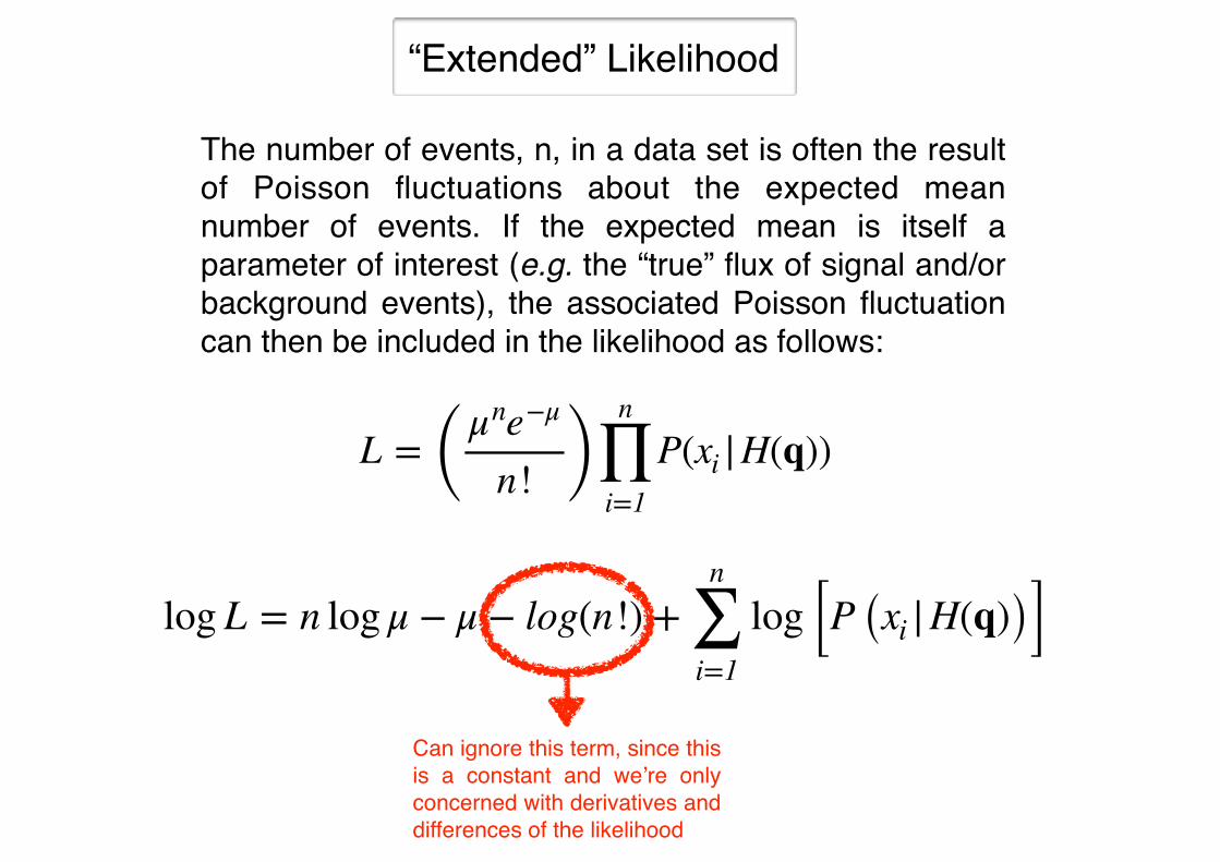
“Extended” Likelihood

The number of events, n, in a data set is often the result of Poisson fluctuations about the expected mean number of events. If the expected mean is itself a parameter of interest (e.g. the “true” flux of signal and/or background events), the associated Poisson fluctuation can then be included in the likelihood as follows:

L = ( μne−μ

n! )n

∏i=1

P(xi |H(q))

log L = n log μ − μ − log(n!) +n

∑i=1

log [P (xi |H(q))]Can ignore this term, since this is a constant and we’re only concerned with derivatives and differences of the likelihood

Example of a 2-component model of signal and background:

An Experiment Searching for Rare Interactions

Reconstructed energy and position could be correlated (e.g. higher energy events could be easier to reconstruct accurately). So, form 2-D histograms to preserve these correlations and normalise these to one to produce PDFs for each type of event class:

“Energy”“Radius”

“Radius” “Energy”

Simulation and/or Calibration Data

signal signal

background background

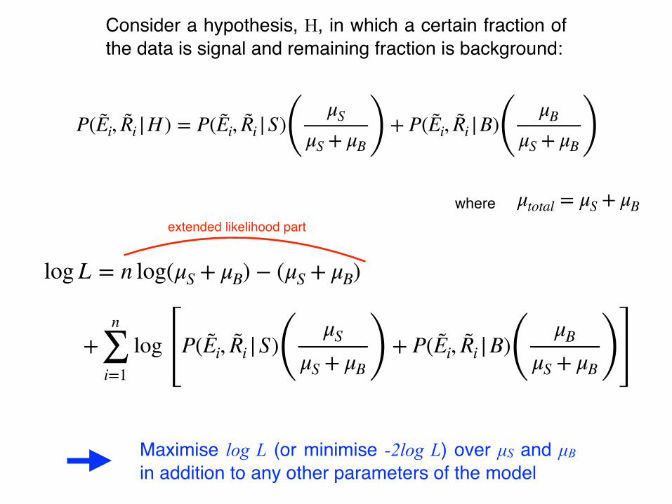
Consider a hypothesis, H, in which a certain fraction of the data is signal and remaining fraction is background:

log L = n log(μS + μB) − (μS + μB)

+n

∑i=1

log P(Ei, Ri |S)( μS

μS + μB ) + P(Ei, Ri |B)( μB

μS + μB )

P(Ei, Ri |H ) = P(Ei, Ri |S)( μS

μS + μB ) + P(Ei, Ri |B)( μB

μS + μB )μtotal = μS + μBwhere

Maximise log L (or minimise -2log L) over µS and µB in addition to any other parameters of the model

extended likelihood part

best esEmate +1σ-1σ

1

0 1 2 3 4 5 6 7 8 9 10

significance

μS

−2 log Lmax

We’re particularly interested in the value and significance of the signal, so look at the projection where the likelihood is maximised over all other free parameters as μS is varied: