Lecture 6: Time Propagation

Outline:

• Ordinary functions of operators

– Powers

– Functions of diagonal operators

• Solving Schrödinger's equation

– Time-independent Hamiltonian

– The Unitary time-evolution operator

– Unitary operators and probability in QM

– Iterative solution

– Eigenvector expansion

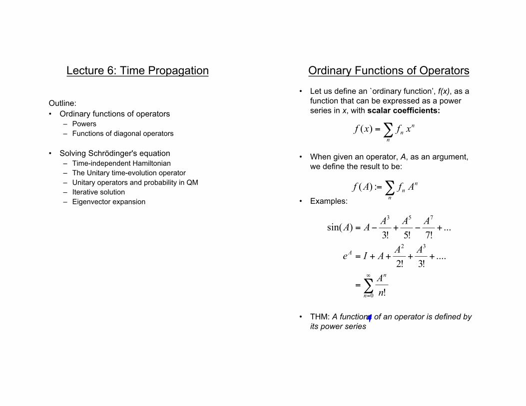
Ordinary Functions of Operators

• Let us define an `ordinary function’, f(x), as a

function that can be expressed as a power

series in x, with scalar coefficients:

• When given an operator, A, as an argument,

we define the result to be:

• Examples:

• THM: A functions of an operator is defined by

its power series

n

n

n xfxf !=)(

n

n

n AfAf !=:)(

!"

=

=

++++=

+#+#=

0

32

753

!

....!3!2

...!7!5!3

)sin(

n

n

A

n

A

AAAIe

AAAAA

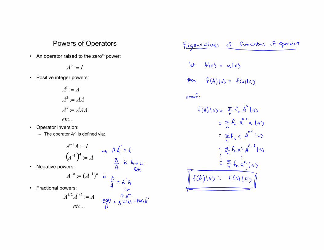
Powers of Operators

• An operator raised to the zeroth power:

• Positive integer powers:

• Operator inversion:

– The operator A-1 is defined via:

• Negative powers:

• Fractional powers:

...

:

:

:

3

2

1

etc

AAAA

AAA

AA

=

=

=

IA =:0

( ) AA

IAA

=

=

!!

!

:

:

11

1

nnAA )(: 1!!

=

...

:2/12/1

etc

AAA =

Functions of Diagonal Operators

• Diagonal operators have the form:

• They can be expressed in Dirac notation as:

• Every operator is diagonal in the basis of

its own eigenvectors

• They have the property:

– let C and D be diagonal matrices

• From which it follows that:

!!!!!!

"

#

$$$$$$

%

&

=

Md

d

d

d

D

L

MOMMM

L

L

L

000

000

000

000

3

2

1

nndD

M

n

n!=

=1

nnd

mmnndcDC

M

n

n

M

n

m

M

m

n

!

!!

=

= =

=

=

1

2

1 1

( )

( )( )

( )

( )!!!!!!

"

#

$$$$$$

%

&

=

Mdf

df

df

df

Df

L

MOMMM

L

L

L

000

000

000

000

3

2

1

Solving Schrödinger’s Equation

• When the Hamiltonian is not explicitly time-

dependent, Schrödinger's Equation is readily

integrated:

– Proof:

)()( tHh

it

dt

d!! "=

)0()( / !! hiHtet"

=

)0(!

)0(0

/ !!m

tHi

dt

de

dt

dmm

m

iHt "#

=

$%&

'()

*$=h

h

)0(!

1

1

!m

mtHi

mm

m

"#

=

$ %&

'()

*"=h

)0()!1(

11

1

!"

#$

%&'

(""=

"")

=

*m

tHi

Hi

mm

m hh

)0(!0

!n

tHi

Hi

nn

n

"#

=

$%

&'(

)**=hh

)0(/ !h

h

iHtHei ""=

)(tHi

!h

"=

The Unitary Time-Evolution Operator

• In general, the time-evolution operator is

defined as:

– The operator U(t,t0) must be Unitary ( U†=U-1 ) topreserve the norm of |!(t)"

• For the case where H is not explicitly time-

dependent, we see from the exact solution

that:

• In the more general case where H=H(t), the

above is not necessarily valid

– In this case we must find an equation for U(t,t0).

– We start from Schrödinger's Equation:

– Which we now write as:

– Since this must be true for any initial state,|!(t0)", it follows that:

)(),()( 00 tttUt !! =

h/)(

00),(ttiH

ettU!!

=

)()( tHh

it

dt

d!! "=

)(),()(),( 0000 tttUHh

itttU

dt

d!! "=

),(),( 00 ttUHh

ittU

dt

d!=

Unitary Operators and probability in QM

Solving the Time-Evolution Operator

Equation

• Since |!(t0)"=U(t0,t0)|!(t0)", it is clear that:

• The equation of motion:

• Can be formally integrated:

• Or re-expressed via the definition of thederivative as:

• With t0=t, this gives infinitesimal time evolutionoperator:

• So that (for numerical purposes):

– Where and

1),( 00 =ttU

),()(),( 00 ttUtHh

ittU

dt

d!=

),()(1),( 00

0

ttUtHtdh

ittU

t

t

!!!"= #

),()(1),(

),()(),(),(

00

000

ttUdttHh

itdttU

ttUtHh

i

dt

ttUtdttU

!"

#$%

&'=+

'='+

dttHh

itdttU )(1),( !=+

!"

#$%

&'!"

#$%

&'!"

#$%

&'=

+++=

()

()

dttHi

dttHi

dttHi

tdttUtdttUtdttUttU

NN

NNN

)(1)(1)(1lim

),(),(),(lim),(

01

00110

hhK

h

K

dtmttm

+=0

Nttdt /)( 0!=

Can this be simplified further?

• We have found the most general result is

• This can be re-written as:

• Note that:

– Only in the case [A,B]=0

• Thus can we write:

– ONLY if the Hamiltonian satisfies:

!"

#$%

&'!"

#$%

&'!"

#$%

&'=

+++=

()

()

dttHi

dttHi

dttHi

tdttUtdttUtdttUttU

NN

NNN

)(1)(1)(1lim

),(),(),(lim),(

01

00110

hhK

h

K

dttHi

dttHi

dttHi

N

eeettUN )()()(

0

12

...lim),( hhh!!!

"#=

BABAeee

+=

)(

00),(

tHtdit

t

ettU

!!" #=

h

[ ] tttHtH !"=! ,0)(),(

Iterative solution:

• We have:

• Start with:

• The iterative form of the equation is:

• Which gives

– Note: the “I” is an integration constant fitted to the

initial conditions

• The final solution is:

),()(),( 00 ttUtHh

ittU

dt

d!=

IttU =),( 00

),()(),( 001 ttUtHh

ittU

dt

dnn

!=+

!"=t

t

tHdti

IttU0

)(),( 1101h

( )

( )

( )

...

)()()(

)()(

)(),(

123123

3

1212

2

110

2

0

3

00

2

00

0

+

+

+

+=

!!!

!!

!

"

"

"

tHtHtHdtdtdt

tHtHdtdt

tHdtIttU

t

t

t

t

t

t

i

t

t

t

t

i

t

t

i

h

h

h

),(),( 00 ttUttU !=

Eigenvector expansion

• For the case where H is not explicitly

time-dependent, it is most common to

use the eigenvector basis to express

the evolution operator.

– The eigenvectors of H are defined by the

eigenvalue equation:

– Note the following:

nnnH !!! h=

n

ti

n

iHt nee !!!""

=h/

mnnm

n

nn

!""

""

=

=# 1

Eigenvector Expansion cont.

• Start from:

• Apply the bra #$n|!:

• Integration then gives:

• We can express the state vector as:

!! Hdt

di =h

)(

)()(

t

tHtdt

di

nn

nn

!""

!"!"

h

h

=

=

)0()( !"!" "

n

ti

n

net#

=

)0(

)()(

!""

!""!

"n

ti

n

n

n

n

n

ne

tt

#$

$

=

=

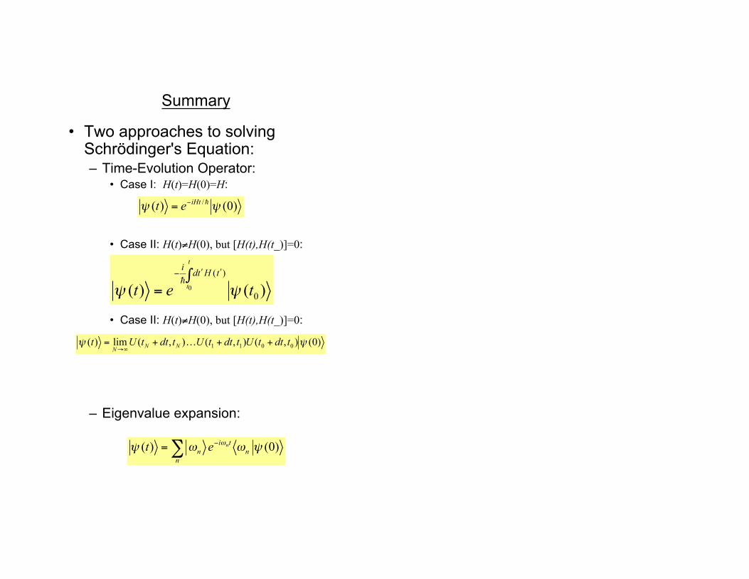
Summary

• Two approaches to solvingSchrödinger's Equation:– Time-Evolution Operator:

• Case I: H(t)=H(0)=H:

• Case II: H(t)%H(0), but [H(t),H(t_)]=0:

• Case II: H(t)%H(0), but [H(t),H(t_)]=0:

– Eigenvalue expansion:

)0()( / !! hiHtet"

=

)0(),(),(),(lim)( 0011 !! tdttUtdttUtdttUtNN

N

+++="#

K

)0()( !""! "n

ti

n

n

net#$=

)()( 0

)(

0 tet

tHtdit

t !!""# $

=h