Lecture 6 The Sun: From the

Core to the Photosphere

Aims, learning outcomes, and overview

Aim: To introduce some of the physics associated with the Sun’s interior andphotosphere, including the energy release and transport processes, and to describeobservational characteristics and modelling approaches of these regions.

Learning outcomes: At the end of this lecture, students are expected to:

• identify and describe qualitatively the different layers of the solar interior,from the core to the photosphere, including the basic physics;

• understand the energy production mechanisms in the Sun and the transportmechanisms of radiation and convection operating inside the Sun;

• describe and explain qualitatively the basic characteristics of sun spots andsolar granulation;

• understand and describe qualitatively the basic techniques and results to dateof helioseismology;

• understand and describe qualitatively mechanisms for magnetic buoyancy anddynamos, and evidence for their operation at the Sun;

• be able to describe recent insights into solar physics provided by solar neutrinomeasurements.

Overview: This lecture presents a survey of some basic physics of the Sun, focusingon the Sun’s interior (from the core to the photosphere), recent developments inhelioseismology and the Sun’s rotation, ideas related to magnetic dynamos andbuoyancy, and recent results involving solar neutrinos.

6.1 Interior structure of the Sun

The structure of the Sun may be divided into the solar atmosphere, i.e. that partof the Sun above the visible surface, or photosphere, and the solar interior. Thesolar interior is divided into the core region, the radiative zone, and the convection

zone, in order of increasing distance from the centre. These divisions are based onthe mechanisms of generation and transport of energy. Figure 6.1 illustrates themultiple layers of the nominal Sun, ranging from the core to the convective zone tothe photosphere and then the various layers to the atmosphere. The photosphere is athin layer in which the solar plasma goes from being almost completely opaque (theinterior) to almost completely transparent (the atmosphere). Because we receive no

1

Figure 6.1: The multiple zones of the nominal Sun, from the solar interior to thecorona. Acoustic wave patterns amenable to helioseismology investigations as wellas magnetic loops are shown.

Quantity ValueRadius R = 6.96× 108 mDistance from Earth 1 AU = 1.50× 1011 mMass M = 1.99× 1030 kgAcceleration at surface g = GM/R2

= 274 m s−1

Luminosity L = 3.86× 1026 J s−1

Photospheric temperature 5762 KSolar age 4.60× 109 years

Table 6.1: Some physical properties of the Sun.

light from below the photosphere, we have limited information about conditions inthe solar interior. Our understanding is based on theoretical models, observationsof solar neutrinos, and inferences from helioseismology. The solar atmosphere isamenable to direct observation in many wavelengths.

Some basic physical properties of the Sun are listed in Table 6.1.

6.1.1 Interior

6.1.1 Core and radiative zone

Fusion of hydrogen to helium is the primary energy production mechanism in theSun, as is well known. This is made possible by the high internal temperature(≈ 1.5 × 107 K) and density (η ≈ 1.6 × 105 kg m−3). The principal set of reactionsinvolves the conversion of Hydrogen into Helium, in three steps called the proton-

proton cycle. A set of reactions involving heavier elements, the CNO cycle alsooccurs.

2

In detail the proton-proton cycle proceeds via the processes

1H +1 H → 2H + e+ + νe + Q1 (6.1)2H +1 H → 3He + γ + Q2 (6.2)

3He +3 He →4 He +1 H +1 H + γ + Q3 . (6.3)

Or alternatively, in summary,

4p+ →4 He2+ + 2e+ + 2νe + 2γ + Q4 . (6.4)

Thus energy is produced in the form of heat, gamma-rays, and electron neutrinos.The simplest approach is to assume that fusion takes place in the innermost

region of the core, with energy transported outwards from there by radiation. How-ever, once suitable hydrogen ions (protons) are exhausted in the core (as a resultof inadequate convection there), fusion is expected to take place in an annular ringthat moves outwards. (Nuclear burning in the ring is typically considered to be rel-evant to stars moving off the Main Sequence towards the asymptotic Giant branch,something that the Sun is not expected to do for several billion years.) Of course,the initial cause for the Sun’s central temperature exceeding the threshold for fusionto occur was due to conversion of gravitation potential energy into thermal energyas the solar nebula condensed and collapsed to form the Sun at its center. Outsidethe burning zone radiation propagates radially outwards, undergoing continual ab-sorption and re-emission so that it is predicted to take in excess of a million yearsfor radiation to travel from the core to the photosphere.

The core and radiative zones can be modelled with fluid equations (usually withthe magnetic terms neglected) that include source terms for energy production (e.g.,fusion) and loss (propagation) on their right hand sides. In these regions thermalpressure and radiation pressure balance the gravitational force.

Models for solar structure begin with the assumption of a hydrostatic balancebetween pressure and gravity [equation (2.37), with only pressure and gravity effectsincluded]:

dP

dr= −

Gmη

r2, (6.5)

where η is the local mass density, and m is the mass inside a sphere of radius r:

dm

dr= 4πr2η. (6.6)

Spherical symmetry is assumed, and the effects of rotation, flows, and magneticfields are ignored. Assuming an ideal gas we have P = NkBT where N is the totalnumber of particles per unit volume and T is the temperature. The mass densitycan be specified in terms of a mean atomic weight µ which is the average mass perparticle in units of the proton mass mH :

η = µmHN, (6.7)

and hence

P =kB

µmHηT. (6.8)

Here N , P , T, and η are all functions of r. More accurate models will also have µa function of r, due to burning of the nuclear fuel.

With the energy produced in the core, near the Sun’s center, the energy andassociated heat energy are expected to flow outward. This leads to a negativetemperature gradient outwards. Eventually as η decreases convection becomes amore important energy transfer mechanism than radiation, leading to a change inbehaviour and the start of the convection zone.

3

6.1.2 Convection zone

In the convective zone energy is transported primarily by convection, with hotterand less dense matter moving up (being buoyant) and cooler and denser materialmoving down. Different source terms are required in this region. Convection cellsvisible at and near the photosphere are directly observable manifestations of theconvection zone. Perhaps even more importantly, though, convection is vital forunderstanding magnetic fields on the Sun. This is due to multiple effects, includingevidence that the convection zone starts at the tachocline, the abrupt and narrowtransition between the convection and radiative zones, the concentration of magneticfields at the boundaries of convection zones (with resultant activity associated withmagnetic reconnection.

Furthermore, there is strong evidence from multiple sources (sun spots, helio-seismology, etc.) that the Sun rotates differentially from the base of the convectionzone to the photosphere (faster at the poles, slower at the equator). This behaviourappears to start at the tachocline and is considered vital for the origin of magneticfields on the Sun.

In the outer part of the Sun’s interior, the convection zone, convective energytransport dominates over radiative transport. Convection is the bulk motion ofa fluid in gas with a sufficient temperature gradient due to a simple instabilitydescribed by Schwarzschild in 1906. Consider a parcel of gas at a radius r withinthe Sun, with temperature T , pressure P and density η, as shown in Figure 6.2.Assume the gas is transported to a radius r + ∆r, where the ambient parametersare T + ∆T , P + ∆P , and η + ∆η. The raised parcel of gas is assumed to havetemperature T +δT , pressure P +δP and density η+δη. If the gas is moved quicklyenough so that the expansion of the parcel is adiabatic (i.e. P ∝ ηΓ, where Γ is theadiabatic index), then

δη

η=

1

Γ

∆P

P, (6.9)

where on the right hand side we have assumed that the lifting of the parcel is slowenough that the gas in the parcel remains in pressure balance with the ambient gas(δP = ∆P ). The parcel will continue to rise due to a buoyancy force if δη < ∆η,or equivalently,

δη

η<

∆η

η. (6.10)

From the ideal gas relationship (P ∝ ηT ),

∆η

η=

∆P

P−

∆T

T. (6.11)

Using equations (6.9) and (6.11) the instability criterion (6.10) may be rewritten as

∆T

T<

Γ − 1

Γ

∆P

P, (6.12)

or in the limit of small displacements,

dT

dr<

Γ − 1

Γ

T

P

dP

dr=

dT

dr

∣

∣

∣

∣

ad

. (6.13)

This is the Schwarzschild stability condition. Both gradients are negative, so thisequation says the parcel of gas will be unstable if the temperature gradient is suf-ficiently negative, i.e. sufficiently steep as a function of radius. Here the final formrepresents the temperature gradient in an ideal adiabatic gas.

In about the outer third of the solar atmosphere the temperature gradient issteeper than the adiabatic value (because the medium’s opacity has increased due

4

Figure 6.2: Set-up for deriva-tion of the Schwarzschild crite-rion for the convective instabil-ity.

to the decreasing temperature), and convection occurs. The actual process of con-vection is a complex dynamic process in which warm gas rises, and then cools andfalls again in convection cells. In a fluid of large viscosity convection cells are regularand stationary, but in the almost inviscid solar gas they become turbulent. Thereis no accepted, fully nonlinear theory for this turbulence, but an approximate “mix-ing length” theory can be developed and shown to yield reasonable agreement withobservations. This theory is not described further here.

Three of the crucial manifestations of the convection zone are the granulationand supergranulation cells visible near the photosphere and the Sun’s magneticfields. These are discussed further below.

6.1.3 A solar model

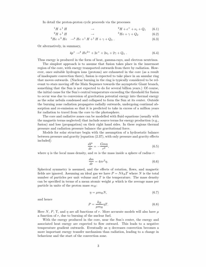
Models for the Sun from the core to the photosphere can then be constructed,typically in the time-stationary, zero average velocity limit. Appropriate conditionsinclude the Sun’s total mass m(R) = M and radiated energy flux (or luminosity)L(R) = L and η(R) = 0. That is the density of material is assumed to bezero at the photosphere. Figure 6.3 illustrates a set of results.

6.2 Photosphere

Figure 6.4 illustrates the output of the Sun across the electromagnetic spectrum.(This figure is at the end of the document.) The Sun’s atmosphere begins with thephotosphere, which is seen in visible light. The radiative output of the Sun peaks inthe visible, and the photospheric spectrum resembles a blackbody at a temperatureof almost 6000 K. However, the Sun’s spectrum in visible light is marked by a seriesof absorption lines called the the Fraunhofer lines. The photosphere is not uniformlybright but exhibits limb darkening, an effect which occurs because the temperatureof the subphotosphere increases with depth. The light we see comes from a fixedoptical depth along the line of sight, and as we move towards the limb, the obliqueincidence of the line of sight with the solar surface means that the originating depthcorresponds to a shallower radial depth into the Sun. Hence the light comes fromcooler material near the limb, and the limb appears darker.

6.2.1 Sunspots

The photosphere is also marked by sunspots, which have been observed sinceGalileo. Sunspots are relatively cool regions compared with the surrounding pho-tosphere, having T ≈ 4000 K. They also have relatively strong magnetic fields atthe surface (up to 0.4 Tesla or 4000 Gauss). It appears that the strong magnetic

5

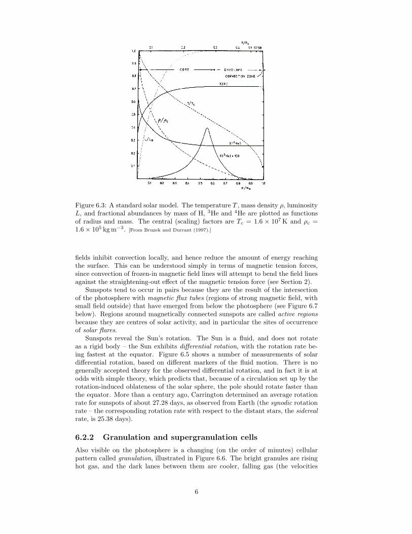
Figure 6.3: A standard solar model. The temperature T , mass density ρ, luminosityL, and fractional abundances by mass of H, 3He and 4He are plotted as functionsof radius and mass. The central (scaling) factors are Tc = 1.6 × 107 K and ρc =1.6 × 105 kg m−3. [From Bruzek and Durrant (1997).]

fields inhibit convection locally, and hence reduce the amount of energy reachingthe surface. This can be understood simply in terms of magnetic tension forces,since convection of frozen-in magnetic field lines will attempt to bend the field linesagainst the straightening-out effect of the magnetic tension force (see Section 2).

Sunspots tend to occur in pairs because they are the result of the intersectionof the photosphere with magnetic flux tubes (regions of strong magnetic field, withsmall field outside) that have emerged from below the photosphere (see Figure 6.7below). Regions around magnetically connected sunspots are called active regions

because they are centres of solar activity, and in particular the sites of occurrenceof solar flares.

Sunspots reveal the Sun’s rotation. The Sun is a fluid, and does not rotateas a rigid body – the Sun exhibits differential rotation, with the rotation rate be-ing fastest at the equator. Figure 6.5 shows a number of measurements of solardifferential rotation, based on different markers of the fluid motion. There is nogenerally accepted theory for the observed differential rotation, and in fact it is atodds with simple theory, which predicts that, because of a circulation set up by therotation-induced oblateness of the solar sphere, the pole should rotate faster thanthe equator. More than a century ago, Carrington determined an average rotationrate for sunspots of about 27.28 days, as observed from Earth (the synodic rotationrate – the corresponding rotation rate with respect to the distant stars, the sidereal

rate, is 25.38 days).

6.2.2 Granulation and supergranulation cells

Also visible on the photosphere is a changing (on the order of minutes) cellularpattern called granulation, illustrated in Figure 6.6. The bright granules are risinghot gas, and the dark lanes between them are cooler, falling gas (the velocities

6

Figure 6.4: The spectrum of the Sun. [From Golub and Pasachoff (1997).]

are around 1 kms−1). Granulation is direct evidence for the turbulent convectionoccurring below the photosphere. Granular diameters appear to follow a continuousdistribution, although they are usually not larger than about 2′′ (≈ 1.4 × 106 m).

There is also a larger scale organisation into supergranules with typical size3 × 107 m, which is visible in doppler velocity measurements of photospheric flows.The borders between supergranules correspond with the sites of emission in certainspectral lines (notably CaII) formed slightly higher in the solar atmosphere: thechromospheric network. The connection is provided by the magnetic field, whichtends to become concentrated in the intra-network lanes by the supergranular flowpattern. For reasons that are not well understood, additional heating occurs in thechromosphere at sites of enhanced magnetic field, as discussed in the next lecture.

6.3 Magnetic dynamos, buoyancy, and photospheric

fields

The magnetic field at the photosphere may be inferred from its effect on spectrallines in the low solar atmosphere – the Zeeman effect. Magnetographs are used toinfer the line of sight magnetic field, and vector magnetographs, or Stokes Polarime-ters may be used to infer the transverse magnetic field.

Flux emerges in sunspot regions because it is buoyant, as argued by Parker andunderstood very simply in terms of pressure balance. As shown in Lectures 2 and5, the Lorentz force may be interpreted as consisting of a magnetic tension andthe gradient of a magnetic pressure, B2/(2µ0), while normal momentum balanceinvolves the ram pressure, thermal pressure, and transverse magnetic field. For astable and static magnetic flux tube there must be a balance normal to the flux

7

Figure 6.5: Differential rotation. Rotation rates for sunspots (NN), photosphericplasma (HH), chromospheric plasma in Hα (L), photospheric magnetic field (WH),coronal plasma (SN), and features in Ca II (SW). [From Bruzek and Durrant (1997).]

Figure 6.6: The photosphere in whitelight, showing small sunspots and gran-ules. [From Stix (1989).]

8

tube’s surface of sum of the thermal fluid pressure and the magnetic pressure insidethe tube, and the thermal pressure outside the tube, neglecting the magnetic fieldoutside the tube and the ram pressure terms. In other words,

Pext = Pint + B2t/(2µ0), (6.14)

where Pint and Pext denote the internal and external gas pressures, respectively,and Bt is the magnetic field in the flux tube. Assuming the temperatures insideand outside the flux tube are equal, and that the fluid obeys the ideal gas equation(P ∝ ηT ), we have that

ηext − ηint

ηext

=B2

2µ0Pe

. (6.15)

Hence ηint < ηext, and the flux tube is buoyant.Figure 6.7) illustrates this process, as well as one effect counteracting it, that

of magnetic tension forces. Convection can also counteract this buoyancy process,especially when the field is weak and the magnetic pressure is small compared withthe thermal and ram pressure terms. The basic point, though, is that the magneticfields tend to be buoyant.

Figure 6.7: A flux tube beneath the photosphere (a). In (b), the flux tube hasemerged, and the regions of intersection with the photosphere may form sunspots.[From Choudhuri (1998).]

Figure 6.7 illustrates, then, why magnetic field lines tend to rise up, form pairsof sun spots, and form magnetic loops in the solar atmosphere. In the photosphereand higher the medium becomes increasingly ionized and the ratio of the magneticenergy density to the thermal energy density becomes large, so that the magneticfield now quantitatively affects the motion of the plasma.

Convection, together with the Sun’s rotation, is thought to be responsible forthe generation of intense localised magnetic fields observed at the surface of the Sun,and hence for solar activity, which is a variety of dynamic phenomena associatedwith magnetic fields. The solar dynamo (the mechanism generating the fields) wasoriginally thought by theorists to reside in the convection zone, but the resultsof helioseismology are inconsistent with the requirements of the models, and thedynamo is now believed to operate at the base of the convection zone, the tachocline,where there are strong radial gradients in the rotation rate. Values for the depth

9

Figure 6.8: Generation of toroidal magnetic field from a poloidal field due to differ-ential rotation. [From Pearson Prentice Hall 2005.]

of the convection zone, derived from helioseismology (§ 6.2), are typically close to0.7R.

Magnetic dynamo theory involves the magnetic induction equation (2.35 in Lec-ture 2)

∂B

∂t= ∇×(U ×B) +

1

µ0σ∇2B , (6.16)

an equation of motion for the magnetized fluid

η

[

∂U

∂t+ (U·∇)U

]

= −∇p + J ×B + ηg . (6.17)

an Ohm’s Law, plus whatever other equations are required to form a closed system.Rotation and convection, including the effects of turbulence, turn out to be vital. InEq. 6.16 the diffusion term is typically a loss term, so that magnetic amplificationinvolves the curl of U ×B term.

A dynamic magnetic dynamo involves flow and magnetic fields that can self-consistently maintain and/or amplify a magnetic field. This is often discussed interms of an α effect and an Ω effect. The Ω effect involves the generation of atoroidal magnetic field from a poloidal field in the presence of differential rotationfor frozen-in fields. This is illustrated in Figure 6.8: the differential rotation pullsthe initially poloidal field into the poloidal direction and wraps it around, generatinga poloidal field.

The re-generation of poloidal field from a toroidal field, the so-called α effectis more complicated. It involves magnetic turbulence that contributes a non-zerotime-averaged current in the Ohm’s Law, with

< J >= σ(< E > + < u > × < B > + < u′ ×B′ >) . (6.18)

When< u′ ×B′ >= α < B > (6.19)

then there is a current along the average magnetic field direction < B > and so amagnetic field is generated transverse to the average magnetic field. This allows apoloidal magnetic field to be generated from a toroidal field.

Thus differential rotation and turbulence appear to be required to form a per-sisting magnetic dynamo. Dynamo theory remains a very active area of research.

10

Figure 6.9: Snapshot of the Sun, showing the convective cells subject to helioseismicoscillations.

6.4 Helioseismology

Helioseismology is an exciting area of solar physics that has developed in the last fewdecades, focusing on wave propagation in the solar interior. The subject derives itsname from the analogy with the study of wave propagation in the Earth’s interior(seismology). Helioseismic observations have allowed accurate measurement of thedepth of the convection zone, as well as inference of the Sun’s internal rotationprofile and internal temperature – measurements that were previously thought tobe impossible to make.

Since 1960 it has been known that the surface of the Sun oscillates, with abouthalf of the Sun (at any time) occupied by oscillatory patches (period ≈ 5 min,amplitude ≈ 1 km s−1). The oscillations last about six or seven periods, and areas aslarge as 30, 000 km often oscillate in phase. Figure 6.9 illustrates these oscillations.

At first this was thought to be a local phenomenon, but now it is known thatthe oscillations are a superposition of global acoustic modes of the Sun. A theoryaccounting for the five-minute oscillations as standing acoustic waves, trapped inthe convection zone was presented by Ulrich and also Leibacher and Stein around1970. The observational confirmation of the theory was made by Deubner in 1975.Figure 6.10 shows one observational indication of the global nature of the modes,namely distinct peaks in the power spectrum of unresolved observations.

Figure 6.10: Power spectrum of global solar oscillations, from 3 months ofintegrated-light observations. [From Phillips (1992).]

11

The theoretical treatment of solar oscillations begins with the linearisation ofthe equation of motion and the continuity equation for perturbations of a gravita-tionally stratified, adiabatic fluid [see Stix (1989) for a more complete description].Rotation and the influence of a magnetic field are neglected in the basic theory.Fluid perturbations are expressed as expansions in spherical harmonics, so that, forexample, the radial component of the fluid displacement is written

ξ(r, t) = exp(iωt)ξr(r)Ym

l(θ, φ). (6.20)

For each degree l, there are many possible eigenfunctions ξr, which are labelled withan integer n, called the order of the mode. The value of n determines the numberof radial nodes in the eigenfunction. The degree l and azimuthal order m define thenumber of node circles on the sphere and the number of node circles passing throughthe poles, as shown in Figure 6.11. On a stationary Sun there are no poles, and sothe eigenfrequencies must be independent of m, a degeneracy that is analogous tothat in the quantum mechanical description of the energy levels of the Hydrogenatom. Rotation introduces a preferred axis and removes this degeneracy, splittingthe eigenfrequencies.

Figure 6.11: Node circles of spherical harmonics. [From Stix (1989).]

The restoring forces for solar oscillations are either pressure or buoyancy (grav-ity). For the 5-minute oscillations pressure is most important, and so the observedoscillations are called p-modes. The modes are thought to be continually excited byturbulence in the convection zone. The modes which have gravity as the restoringforce are called g-modes. Calculation suggests that these modes are predominantlytrapped in the solar interior, and are not detectable at the solar surface. Thereis considerable interest in the possibility of detecting g modes and using them forseismology, because they probe the deep interior of the Sun, but to date there hasbeen no generally accepted detection. There are also surface waves, called f-modes.

There are two observational approaches in helioseismology. Doppler measure-ments with no spatial resolution may be used to determine the signal of low-l modes.High-l modes require spatial resolution. The best helioseismic measurements todate have come from the Michelson Doppler Interferometer (MDI) instrument onthe Solar and Heliospheric Observer (SOHO) spacecraft.

Because the mode frequencies depend on the internal sound speed of the Sun,it is possible to take the observed spectrum of frequencies and solve the inverseproblem to obtain the sound speed as a function of radius. Figure 6.12 shows anexample, together with the sound speed predicted by a solar model. The curvesagree almost to within the thickness of the line (although in fact they disagreemore than the estimated errors). The base of the convection zone is detectable as achange in curvature at about 0.7R. The inversions are quite reliable, and confirmthe structure predicted by standard stellar evolution theory.

12

Figure 6.12: The inter-nal sound speed of theSun, inferred from he-lioseismology data, to-gether with sound speedpredicted by a standardsolar model. The agree-ment is within the thick-ness of the lines in thelarger picture. [From Deub-

ner & Gough (1984).]

The degree of splitting of the p-modes depends on the internal rotation of theSun. It is also possible to take the observed splittings and infer how the rotationrate varies inside the Sun. Figure 6.13 shows an example. The main featuresof the inferred rotation profile are that differential rotation ends at the base of theconvection zone, i.e. the radiative zone and core rotate (almost) rigidly, and that therotation in the convection zone is almost constant along radial lines. Hydrodynamicmodels of rotation have considerable difficulty accounting for these basic features.

Finally we mention a recent development, local helioseismology. By examiningthe correlations of p-mode oscillations on the surface of the Sun observed at highresolution, it is possible to infer the local variation of sound speed with depth. Itis also possible to infer the magnetic field as a function of position below sunspotsusing “sunquakes” and other localized sources of waves.

6.5 Solar neutrino observations and arguments for

fusion

Until early in the 20th century, it was believed that the Sun was continually col-lapsing, releasing gravitational potential energy in the process, and this process wasthought to power the Sun. The total gravitational potential energy of the Sun isabout

Ω = −GM2/R ≈ −4 × 1041 J, (6.21)

and the present luminosity of the Sun is L ≈ 3.9 × 1026 W. Assuming continualconversion of gravitational potential energy to solar output, at its present luminositythe Sun would last about the Kelvin-Helmholtz time,

τKH = Ω/L ≈ 1015 s ≈ 3 × 107 y. (6.22)

Hence until the early 1900s it was believed that the Sun and the Earth are a few tensof million years old. However, geological evidence pointed to a much older Earth

13

Figure 6.13: (Left) The internal rotation profile of the Sun, inferred from GONGhelioseismology. The units are nano-Hz. (Right) Cuts at different heliolatitudes forthe rotation rate as a function of radial distance, also from GONG.

14

(the currently accepted age for the Sun and the Earth is about 4.6×109 y). In 1929Eddington was among the first to argue that the Sun must be fueled by a subatomicsource of energy. A detailed theoretical explanation of the nuclear processes occur-ring in the Sun’s core was provided by Hans Bethe in 1939, although because thetemperature of the interior was thought to be higher than the accepted value today,Bethe favoured the CNO cycle as the dominant process. The final confirmation ofthe fusion hypothesis was the observational detection of solar neutrinos, which areproduced by the nuclear reactions in the Sun’s core.

Neutrinos are fundamental particles that have no charge and have a very small(or zero) mass. They interact only via the weak force, and the cross section forinteraction is very small, so matter is effectively transparent to neutrinos. Anenormous number of neutrinos are produced in the core of the Sun – of order1038 s−1. The longest-running experiment to detect solar neutrinos was started byRay Davies in 1967. The experiment is 1.5 km underground in the Homestake minein South Dakota, and consists of a tank containing 380,000 litres of cleaning fluid.The fluid contains a large number of Chlorine atoms. About every two days, oneChlorine atom undergoes the reaction

νe + 37Cl → e− + 37Ar. (6.23)

The 37Ar atom produced is subsequently detected by its decay back to 37Cl.After the Homestake experiment had been run for some time, it was realised that

too few neutrinos were being observed (by about a factor of three), compared withthe predictions from standard solar models. The observed deficit was known as thesolar neutrino problem. Figure 6.14 illustrates the results from the Homestake ex-periment and the theoretical predictions for that experiment (far left, labelled ‘Cl’).Subsequent solar neutrino experiments confirmed the deficit and its approximatevalue. The Japanese Kamiokande experiment (and the later Super-Kamiokande)used the scattering of neutrinos on electrons via detection of the Cerenkov radi-ation produced by the electrons. These experiments gave information about thedirection of flight of the neutrinos, and confirmed that the observed neutrinos comefrom the Sun.

The solar neutrino problem indicated a deficiency in either the understandingof the Sun (and hence of stellar modelling), or in the standard model for neutrinos.However, the consistency of solar models with heliospheric results suggested that theproblem was with the neutrino. According to the standard particle physics model,there are three varieties (flavours) of neutrino: the electron, tau, and mu neutrino.Solar neutrinos are generated as electron neutrinos, and only electron neutrinos aredetected by the Homestake and Kamiokande experiments. However, if the neutrinochanges its flavour enroute to Earth (oscillate), a deficit in neutrinos would beobserved. Further, if a neutrino is equally likely to arrive at Earth as any flavour,i.e. if there is strong mixing, then the detected flux would be reduced by a factorof three, reconciling theory and observations. For oscillations to occur, neutrinosrequire a finite rest mass, but the standard particle physics model says that theneutrino rest mass is zero. Recently, experimental evidence for neutrino oscillationswas obtained. The Sudbury Neutrino Observatory (SNO) has simultaneously runan experiment sensitive to only electron neutrinos and an experiment sensitive toall three neutrino flavours (Ahmad et al. 2002). The inferred flux for the secondexperiment was three times that of the first experiment, consistent with strongmixing. The total flux of neutrinos was found to be consistent with the standardsolar model, so that the neutrino problem finally appears to have been resolved. In2002 the Nobel Prize in Physics was partly awarded to Ray Davis and to MasatoshiKoshiba, the leader of the original Kamiokande experiment.

15

SAGE GALLEX

+GNOSuperK

Kamiokande

SNO SNO

Figure 6.14: Solar neutrino flux measurements from a variety of experiments andtheoretical predictions. On the far left are the original measurements from theHomestake experiment, and the theoretical predictions for that experiment. Resultsfor the Sudbury Neutrino Observatory (SNO) are shown at the far right. Theseresults appear to solve the solar neutrino problem. [From John Bahcall’s web pages:http://www.sns.ias.edu/∼jnb/.]

References

Ahmad, Q.R., et al. 2002, Phys. Rev. Lett., 89, 011301

Bahcall, J.N. 1989, Neutrino Astrophysics, Cambridge University Press, Cambridge

Bowers, R.L. and Deeming, T. 1984, Astrophysics I: Stars, Jones and Bartlett, Boston

Bruzek, A. and Durrant, C.J. (eds.) 1977, Illustrated Glossary for Solar and Solar-

terrestrial Physics, D. Reidel, Dordrecht

Choudhuri, A.R. 1998, The Physics of Fluids and Plasma: An Introduction for Astrophysi-

cists, Cambridge University Press, Cambridge

Cox, A.N., Livingston, W.C. and Matthews, M.S. (eds.) 1991, Solar Interior and Atmo-

sphere, University of Arizona Press, Tucson

Deubner, F.L. and Gough, D. 1984, Annual Reviews of Astronomy and Astrophysics 32,593

Gibson, E.G. 1973, The Quiet Sun, NASA SP-303

Golub, L. and Pasachoff, J.M. 1997, The Solar Corona, Cambridge University Press, Cam-bridge

Phillips, K. 1992, Guide to the Sun, Cambridge University Press, Cambridge

Stix, M. 1989, The Sun: An Introduction, Springer-Verlag, Berlin

16