Lecture 6 guidelines_and_assignment

Introduction to Applied Statistics and Applied Statistical Methods Practical guidelines

Prof. Dr. Chang Zhu page 1

Table of Contents

LECTURE 6 ..................................................................................................................................................... 2

LINEAR REGRESSION ..................................................................................................................................... 2

MULTIPLE REGRESSION ................................................................................................................................. 3

SPSS OUTPUT ............................................................................................................................................ 5

HYPOTHESIS TESTING ................................................................................................................................ 5

REPORT THE RESULTS ............................................................................................................................... 8

MODEL GENERALIZATION ......................................................................................................................... 9

ASSIGNMENT 6 ............................................................................................................................................ 13

References .................................................................................................................................................. 13



LECTURE 6

LINEAR REGRESSION

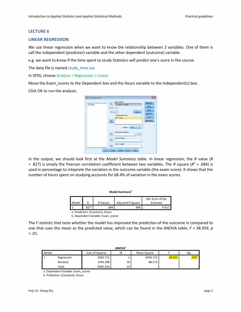
We use linear regression when we want to know the relationship between 2 variables. One of them is call the independent (predictor) variable and the other dependent (outcome) variable.

e.g. we want to know if the time spent to study Statistics will predict one’s score in the course.

The data file is named study_time.sav

In SPSS, choose Analyse > Regression > Linear

Move the Exam_scores to the Dependent box and the Hours variable to the Independent(s) box.

Click OK to run the analysis.

In the output, we should look first at the Model Summary table. In linear regression, the R value (R = .827) is simply the Pearson correlation coefficient between two variables. The R square (R2 = .684) is used in percentage to inteprete the variation in the outcome variable (the exam score): It shows that the number of hours spent on studying accounts for 68.4% of variation in the exam scores.

Model Summaryb

Model R R Square Adjusted R Square Std. Error of the

Estimate

1 .827a .684 .666 9.411

a. Predictors: (Constant), Hours b. Dependent Variable: Exam_scores

The F-statistic that tests whether the model has improved the prediction of the outcome in compared to one that uses the mean as the predicted value, which can be found in the ANOVA table, F = 38.959, p < .01.

ANOVAa

Model Sum of Squares df Mean Square F Sig.

1 Regression 3450.712 1 3450.712 38.959 .000b

Residual 1594.308 18 88.573

Total 5045.020 19

a. Dependent Variable: Exam_scores b. Predictors: (Constant), Hours



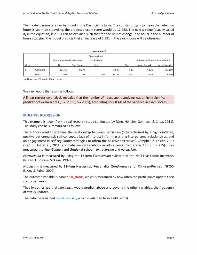
The model parameters can be found in the Coefficients table. The constant (b0) is to mean that when no hours is spent on studyding, the predicted exam score would be 12.762. The next b value (usually called b1 in the equation) is 2.391 can be explaied such that for one unit of change (one hour) in the number of hours studying, the model predicts that an increase of 2.391 in the exam score will be observed.

We can report the result as follows:

A linear regression analysis revealed that the number of hours spent studying was a highly significant

predictor of exam scores ( = .2.391, p = < .01), accounting for 68.4% of the variance in exam scores.

MULTIPLE REGRESSION

This example is taken from a real research study conducted by (Ong, Ho, Lim, Goh, Lee, & Chua, 2011). The study can be summarized as follow:

The authors want to examine the relationship between narcissism (“characterized by a highly inflated, positive but unrealistic self-concept, a lack of interest in forming strong interpersonal relationships, and an engagement in self-regulatory strategies to affirm the positive self-views”, Campbell & Foster, 2007 cited in Ong et al., 2011) and behavior on Facebook in adolescents from grade 7 to 9 (n= 275). They measured the Age, Gender, and Grade (at school), extraversion and narcissism.

Extraversion is measured by using the 12-item Extraversion subscale of the NEO Five-Factor Inventory (NEO-FFI, Costa & McCrae, 1992a)

Narcissism is measured by 12-item Narcissistic Personality Questionnaire for Children-Revised (NPQC-R, Ang & Raine, 2009).

The outcome variable is named FB_status, which is measured by how often the participants update their status per week.

They hypothesized that narcissism would predict, above and beyond the other variables, the frequency of status updates.

The data file is named narcissism.sav, which is adapted from Field (2013).

Coefficientsa

Model

Unstandardized Coefficients

Standardized

Coefficients

t Sig.

95.0% Confidence Interval for B

B Std. Error Beta Lower Bound Upper Bound

1 (Constant) 12.762 8.276 1.542 .140 -4.625 30.150

Hours 2.391 .383 .827 6.242 .000 1.586 3.196

a. Dependent Variable: Exam_scores

http://www.sciencedirect.com.ezproxy.vub.ac.be:2048/science/article/pii/S0191886910004654#b0030





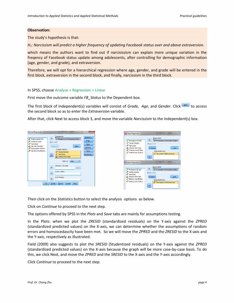
Observation:

The study’s hypothesis is that:

H1: Narcissism will predict a higher frequency of updating Facebook status over and above extraversion.

which means the authors want to find out if narcisissism can explain more unique variation in the freqency of Facebook status update among adolescents, after controlling for demographic information (age, gender, and grade), and extraversion.

Therefore, we will opt for a hierarchical regression where age, gender, and grade will be entered in the first block, extraversion in the second block, and finally, narcissism in the third block.

In SPSS, choose Analyse > Regression > Linear

First move the outcome variable FB_Status to the Dependent box.

The first block of Independent(s) variables will consist of Grade, Age, and Gender. Click to access the second block so as to enter the Extraversion variable.

After that, click Next to access block 3, and move the variable Narcissism to the Independent(s) box.

Then click on the Statistics button to select the analysis options as below.

Click on Continue to proceed to the next step.

The options offered by SPSS in the Plots and Save tabs are mainly for assumptions testing.

In the Plots: when we plot the ZRESID (standardized residuals) on the Y-axis against the ZPRED (standardized predicted values) on the X-axis, we can determine whether the assumptions of random errors and homoscedascity have been met. So we will move the ZPRED and the ZRESID to the X-axis and the Y-axis, respectively as illustrated.

Field (2009) also suggests to plot the SRESID (Studentized residuals) on the Y-axis against the ZPRED (standardized predicted values) on the X-axis because the graph will be more case-by-case basis. To do this, we click Next, and move the ZPRED and the SRESID to the X-axis and the Y-axis accordingly.

Click Continue to proceed to the next step.



The dialog box named Save (Saving regression analysis) helps us to evaluate how well our model fits the data and to detect any cases that have an influence on the model. Select the options as suggested, then click Continue to proceed to the next step.

The Option dialog box provides us with the option to choose the probability level for our analysis as well as whether to include a constant in the regression equation. For missing values, the recommended option is Exclude cases listwise.

SPSS OUTPUT

HYPOTHESIS TESTING

As with linear regression, we will look at 3 tables: Model Summary, Anova, and Coefficients to come up with the conclusion.

As we entered the variables in 3 blocks with the first block being the variables that have already been confirmed, and the final (third) block being the variable (Narcissism) of our interest, we will find 3 models in the Model Summary table:

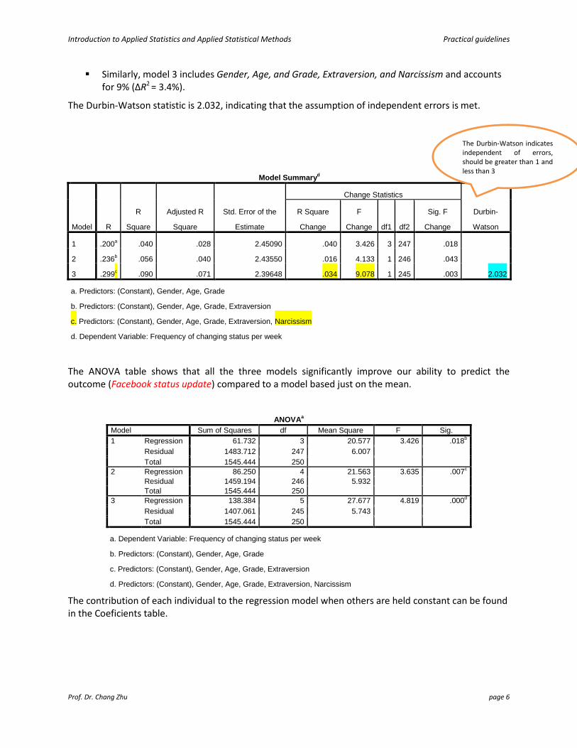
Model 1 includes Gender, Age, and Grade as predictors, and accounts for 4% in the variation in Facebook status update.

Model 2 includes Gender, Age, and Grade, and Extraversion, and accounts for 5.6% in the variation (R squared change indicated as ΔR2 is equal to 1.6%).



Similarly, model 3 includes Gender, Age, and Grade, Extraversion, and Narcissism and accounts for 9% (ΔR2 = 3.4%).

The Durbin-Watson statistic is 2.032, indicating that the assumption of independent errors is met.

Model Summaryd

Model R

R

Square

Adjusted R

Square

Std. Error of the

Estimate

Change Statistics

Durbin-

Watson

R Square

Change

F

Change df1 df2

Sig. F

Change

1 .200a .040 .028 2.45090 .040 3.426 3 247 .018

2 .236b .056 .040 2.43550 .016 4.133 1 246 .043

3 .299c .090 .071 2.39648 .034 9.078 1 245 .003 2.032

a. Predictors: (Constant), Gender, Age, Grade

b. Predictors: (Constant), Gender, Age, Grade, Extraversion

c. Predictors: (Constant), Gender, Age, Grade, Extraversion, Narcissism

d. Dependent Variable: Frequency of changing status per week

The ANOVA table shows that all the three models significantly improve our ability to predict the outcome (Facebook status update) compared to a model based just on the mean.

ANOVAa

Model Sum of Squares df Mean Square F Sig.

1 Regression 61.732 3 20.577 3.426 .018b

Residual 1483.712 247 6.007

Total 1545.444 250

2 Regression 86.250 4 21.563 3.635 .007c

Residual 1459.194 246 5.932

Total 1545.444 250

3 Regression 138.384 5 27.677 4.819 .000d

Residual 1407.061 245 5.743

Total 1545.444 250

a. Dependent Variable: Frequency of changing status per week

b. Predictors: (Constant), Gender, Age, Grade

c. Predictors: (Constant), Gender, Age, Grade, Extraversion

d. Predictors: (Constant), Gender, Age, Grade, Extraversion, Narcissism

The contribution of each individual to the regression model when others are held constant can be found in the Coeficients table.

The Durbin-Watson indicates independent of errors, should be greater than 1 and less than 3



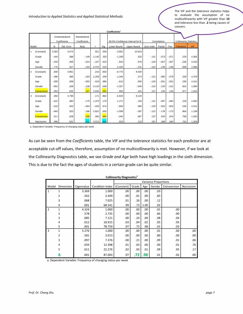
As can be seen from the Coefficients table, the VIF and the tolerance statistics for each predictor are at

acceptable cut-off values, therefore, assumption of no multicollinearity is met. However, if we look at

the Collinearity Diagnostics table, we see Grade and Age both have high loadings in the sixth dimension.

This is due to the fact the ages of students in a certain grade can be quite similar.

Collinearity Diagnosticsa

Model Dimension Eigenvalue Condition Index

Variance Proportions

(Constant) Grade Age Gender Extraversion Narcissism

1 1 3.369 1.000 .00 .00 .00 .03

2 .562 2.449 .00 .01 .00 .83

3 .068 7.025 .01 .26 .00 .12

4 .001 68.541 .99 .73 1.00 .02

2 1 4.324 1.000 .00 .00 .00 .01 .00

2 .578 2.735 .00 .00 .00 .84 .00

3 .085 7.121 .00 .24 .00 .08 .04

4 .012 18.915 .03 .04 .02 .05 .93

5 .001 78.759 .97 .72 .98 .01 .03

3 1 5.276 1.000 .00 .00 .00 .01 .00 .00

2 .581 3.013 .00 .00 .00 .80 .00 .00

3 .097 7.376 .00 .21 .00 .09 .01 .06

4 .034 12.398 .01 .03 .00 .00 .01 .76

5 .011 22.276 .02 .03 .01 .09 .95 .17

6 .001 87.003 .97 .72 .98 .01 .02 .00


Coefficientsa

Model

Unstandardized

Coefficients

Standardized

Coefficients

t Sig.

95.0% Confidence Interval for B Correlations Collinearity Statistics

B Std. Error Beta Lower Bound Upper Bound Zero-order Partial Part Tolerance VIF

1 (Constant) 3.383 3.674 .921 .358 -3.852 10.619

Grade -.444 .388 -.149 -1.145 .253 -1.208 .320 -.131 -.073 -.071 .229 4.365

Age -.033 .309 -.014 -.107 .915 -.642 .576 -.129 -.007 -.007 .236 4.233

Gender -.775 .327 -.153 -2.370 .019 -1.420 -.131 -.122 -.149 -.148 .936 1.068

2 (Constant) .830 3.861 .215 .830 -6.775 8.434

Grade -.486 .386 -.163 -1.259 .209 -1.246 .274 -.131 -.080 -.078 .228 4.378

Age -.006 .308 -.002 -.019 .985 -.612 .600 -.129 -.001 -.001 .236 4.241

Gender -.691 .328 -.136 -2.110 .036 -1.337 -.046 -.122 -.133 -.131 .921 1.085

Extraversion .052 .025 .127 2.033 .043 .002 .101 .137 .129 .126 .977 1.024

3 (Constant) .650 3.799 .171 .864 -6.833 8.134

Grade -.522 .380 -.175 -1.375 .170 -1.271 .226 -.131 -.087 -.084 .228 4.382

Age -.010 .303 -.004 -.033 .974 -.606 .586 -.129 -.002 -.002 .236 4.241

Gender -.943 .333 -.186 -2.831 .005 -1.599 -.287 -.122 -.178 -.173 .864 1.158

Extraversion .011 .028 .028 .394 .694 -.045 .067 .137 .025 .024 .758 1.320

Narcissism .066 .022 .212 3.013 .003 .023 .110 .187 .189 .184 .752 1.329


The VIF and the tolerance statistics helps to evaluate the assumption of no multicollinearity with VIF greater than 10 and tolerance less than .2 being causes of concern.



If we look at model 3, i.e. after controlling for grade, age, gender, it’s found that narcissism significantly

predicts the frequency of Facebook status update over and above/beyond extraversion (β = .21, p <.01)

REPORT THE RESULTS

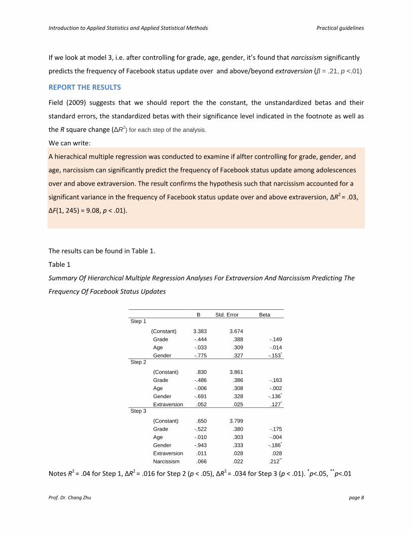
Field (2009) suggests that we should report the the constant, the unstandardized betas and their

standard errors, the standardized betas with their significance level indicated in the footnote as well as

the R square change (ΔR2) for each step of the analysis.

We can write:

A hierachical multiple regression was conducted to examine if alfter controlling for grade, gender, and

age, narcissism can significantly predict the frequency of Facebook status update among adolescences

over and above extraversion. The result confirms the hypothesis such that narcissism accounted for a

significant variance in the frequency of Facebook status update over and above extraversion, ΔR2 = .03,

ΔF(1, 245) = 9.08, p < .01).

The results can be found in Table 1.

Table 1

Summary Of Hierarchical Multiple Regression Analyses For Extraversion And Narcissism Predicting The

Frequency Of Facebook Status Updates

B Std. Error Beta

Step 1

(Constant) 3.383 3.674

Grade -.444 .388 -.149

Age -.033 .309 -.014

Gender -.775 .327 -.153*

Step 2

(Constant) .830 3.861

Grade -.486 .386 -.163

Age -.006 .308 -.002

Gender -.691 .328 -.136*

Extraversion .052 .025 .127*

Step 3

(Constant) .650 3.799

Grade -.522 .380 -.175

Age -.010 .303 -.004

Gender -.943 .333 -.186*

Extraversion .011 .028 .028

Narcissism .066 .022 .212**

Notes R2 = .04 for Step 1, ΔR2 = .016 for Step 2 (p < .05), ΔR2 = .034 for Step 3 (p < .01). *p<.05, **p<.01



MODEL GENERALIZATION

To evaluate whether we generalize our model to make generalization about a different

sample/population we should look at the following graphs that we have requested in the analysis.

The first two are the histogram and the normal probability plot with the standardized predicted values

(ZPRED) against the standardized residuals (ZRESID). As can be seen, the histogram and the P-P plot

show that deviation from normality has been found.

The scatter plots also indicate that there is problem of heteroscedasticity in the data. Field notes that “In

a situation in which the assumptions of linearity and homoscedasticity are met, the points are randomly

and evenly dispersed throughout the plot” (p. 247). So the scatter plots obtained from the study’s data

demonstrate that the distribution of residuals are not random, but follow almost a certain linear pattern.

So the assumption of homoscedasticity has not been met.



Next comes the 5 partial scatterplots of the residuals of the outcome variable (FB status update) and

each of the five predictors (grade, age, gender, extraversion, and narcissism). We can also identify any

outliers if any in the partial scatterplots. Here we just look at 2 partial scatter plots as an example, and

we notice: (1) there a linear relationship between the gender, narcissism and the Facebook update

status; (2) there are 2 outliers.

Actually, we can already identify which are the outliers in the table named Casewise Diagnostics. In this

case, they are case 131 and 231 because we can see that their Facebook status update per week is 14

while the model predicts just 2.31 (residual = 11.68) and 2.26 (residual = 11.73) accordingly.

Casewise Diagnosticsa

Case Number Std. Residual

Frequency of

changing status

per week Predicted Value Residual

131 4.878 14.00 2.3104 11.68955

231 4.896 14.00 2.2676 11.73244


To see if these two cases will have significant influence on the accuracy of our regression model we will

examine if they exceed the conventional cut-off values of the following influential statistics (Field, 2009):

Calculate the average leverage (number of predictor plus 1, divided by the sample size or

(k+1)/n), look for value greater than two or three times this average value. So for our data, the

leverage value is (5+1)/251=0.024

Cook’s distance: value above 1 indicates an influencing case.

Mahalanobis distance, value above 15 (sample size = 100) is cause of concern.

Absolute DFbeta greater than 1 is a problem.

Standardized DFFit as close to zero indicates good fit.



Calculate the upper and lower limit of acceptable values for the covariance ratio (CVR), using the

following equations. Any cases outside these limits are a problem.

upper limit for CVR: 1 + 3(k+1)/n = 1 + 3(5+1)/251 = 1.071

lower limit for CVR: 1 - 3(k+1)/n = 1 - 3(5+1)/251 = 0.928

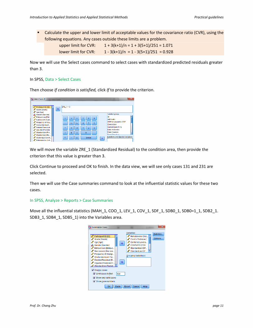
Now we will use the Select cases command to select cases with standardized predicted residuals greater

than 3.

In SPSS, Data > Select Cases

Then choose If condition is satisfied, click If to provide the criterion.

We will move the variable ZRE_1 (Standardized Residual) to the condition area, then provide the

criterion that this value is greater than 3.

Click Continue to proceed and OK to finish. In the data view, we will see only cases 131 and 231 are

selected.

Then we will use the Case summaries command to look at the influential statistic values for these two

cases.

In SPSS, Analyze > Reports > Case Summaries

Move all the influential statistics (MAH_1, COO_1, LEV_1, COV_1, SDF_1, SDB0_1, SDB0=1_1, SDB2_1.

SDB3_1, SDB4_1, SDB5_1) into the Variables area.



Under the Display cases area, choose the options as suggested, then click OK to finish. In the output, we

can compare the influential statistics for the two cases with the cut-off values.

As obtained from the Case Summaries table, the two cases satisfy most of the criteria, except for the

Covariance Ratio and the standardized DFFit. Therefore, we can keep these two cases because according

to Field (2009), the Cook’s and the Mahalanobis distance for the two cases are acceptable, indicating

that they can cause a little, but not big influence on the regression model.

Case Summariesa

cases

Mahalanobis

Distance

Cook's

Distance

Centered

Leverage

Value COVRATIO

Standardized

DFFIT

Standardized

DFBETA

Intercept

Standardized

DFBETA

Grade

Standardized

DFBETA

Age

Standardized

DFBETA

Gender

Standardized

DFBETA

Extraversion

Standardized

DFBETA

Narcissism

131 3.99529 .08243 .01598 .55911 .73942 -.13512 .14031 -.01917 -.18263 .32825 .21441

231 1.53312 .04124 .00613 .55452 .52294 -.07824 -.09206 .03514 -.23134 .26096 -.02360

Total N 2 2 2 2 2 2 2 2 2 2 2

a. Limited to first 100 cases.

Conclusion: Using a number of diagnostic statistics to check accuracy of the model (the Durbin-Watson,

the VIF, the tolerance, the histogram, P-P plot, and scatter plots) and the influential cases, we can see

that the model fails to meet certain assumptions, especially the normal distribution of residuals and the

homoscedasticity. Therefore, we cannot generalize our model for the population. This is in accordance

with the limitations that Ong, Ho, Lim, Goh, Lee, and Chua (2011) have indicated in their paper.



ASSIGNMENT 6

(You can work alone or in group for this assignment. If you work in group, please stay in the same group of previous assignments and indicate the group members in the submission document).

We know from the Collinearity Diagnostics that age and grade are highly correlated so, it can be

redundant to include both in the regression model and also can affect the accuracy of the model.

Therefore, we will only retain Age in this assignment and see if there can be any improvement in the

regression model.

For this assignment, you’ll try to test the following hypothesis:

H1: Narcissism will predict a higher rating of one’s own profile photo over and above extraversion.

which means you will find out if narcisissism can explain more unique variation in rating of Facebook profile photo (profile_photo_rating) among adolescents, after controlling for demographic information (age and gender), and extraversion.

When reporting the results, you should include the following:

- A paragraph describe what method of regression you used, the variables included, which

hypothesis to test and whether it is supported with the R square and F change and the

significant p value.

- A table of report includes the constant, the unstandardized betas and their standard errors,

the standardized betas with their significance level indicated in the footnote as well as the R

square change (ΔR2) for each step of the analysis.

- Check if your model can be generalized by: looking at the histogram and the normal probability plot with the standardized

predicted values (ZPRED) against the standardized residuals (ZRESID), and the scatter plots;

analyzing if there are any influential outliers (criteria: value greater than 3 standard deviations, see how to obtain this on page 5). If you remove the outlier from the data set, re-run the analysis.

- Come up with a conclusion paragraph to see if the model can be generalized.

The data file is named narcissism.sav.

References

Field, A. (2009). Discovering statistics using SPSS. Sage publications.

Field, A. (2013). Discovering statistics using IBM SPSS Statistics. Sage publications

Ong, E. Y., Ho, J., Lim, J. C., Goh, D. H., Lee, C. S., & Chua, A. Y. (2011). Narcissism, extraversion and adolescents’ self-presentation on Facebook. Personality and Individual Differences, 50(2), 180-185.

Lecture 6 guidelines_and_assignment

Documents

Transcript of Lecture 6 guidelines_and_assignment