Lecture 6 Brittle Deformation - · PDF fileBrittle deformation is the permanent change that...

Brittle Deformation

Earth Structure (2nd Edition), 2004

W.W. Norton & Co, New York

Slide show by Ben van der Pluijm

© WW Norton, unless noted otherwise

Lecture 6

Brittle deformation

© EarthStructure (2nd ed) 29/23/2014

Types of brittle deformation Figure 6.4


Brittle deformation is the permanent change that occurs in a solid material due to the growth of fractures and/or due to sliding on fractures once they have formed.

Tensile Shear

crack fracture

A shear fracture, forming at an angle of about 30°to the σ1 direction. (d) A tensile crack that has been reoriented with respect to the remote stresses and becomes a fault by undergoing frictional sliding.

Orientation of the remote principal stress directions with respect to an intact rock body.

A tensile crack, forming parallel to σ1 and perpendicular to σ3

(which may be tensile).

A tensile crack that has been reoriented with respect to the remote stresses and becomes a fault by undergoing frictional sliding.

A tensile crack which has been reactivated as a

cataclastic shear zone.

A shear fracture that has evolved into a fault.

A shear fracture that has evolved into a cataclasticshear zone.

Brittle Deformation Processes



Atomic perspective

Strength Paradox: Rocks allow only few % elastic strain before ductile or brittle deformation.

σ = E . E = 1011 . 0.1 = 1010 Pa

Thus, theoretical strength is 1000’s Mpa

Practical strength 10’s MPa

FIGURE 6.3 A sketch illustrating what is meant by stretching and breaking of atomic bonds.

FIGURE 6.5 A cross-sectional sketch of a crystal lattice (balls are atoms and sticks are bonds) in which there is a crack. The crack is a plane of finite extent across which all atomic bonds are broken.

Four atoms arranged in a lattice at equilibrium.

The chemical bonds are represented by springs and

the atoms by spheres.

As a consequence of stretching of the lattice, some bonds stretch and

some shorten, and the angle between pairs of bonds changes.

If the bonds are stretched too far, they break, and elastic

strain is released

Tensile cracking Figures 6.6 and 6.7


Remote and local stress: stress concentration, C, is (2b/a) +1

Crack 1 x .02 µm: C = 100 ! - C becomes larger as cracks grow (larger is weaker) - cracks ‘runaway’

Stress concentration adjacent to a hole in an elastic sheet. If the sheet is subjected to a remote tensile stress at its ends (σr), then stress magnitudes at the sides of the holes are equal to Cσr, where the

stress concentration factor (C), is (2b/a) + 1.

For a circular hole, C = 3. For an elliptical hole, C > 3.

Illustration of a home experiment to

observe the importance of preexisting cracks in creating stress concentrations.

The larger preexisting cut propagates.

In the shaded area, a region called the process zone, the plastic strength of the material is exceeded and deforms.

An intact piece of paper is difficult to pull apart.

Two cuts, a large one and a small one, are made in the paper.

Axial experiments: Griffith cracks Figs. 6.8 and 6.9


Effect of preexisting (or Griffith) cracks: preferred activation

Development of a through-going crack in a block under tension.

When tensile stress (σt) is applied, Griffith

cracks open up

The largest, properly oriented cracks propagate

to form a through going crack.

Extension Compression

A cross section showing a rock cylinder with mesoscopic

cracks formed by the process of longitudinal splitting.

If you push down on the top of an envelope (whose ends have been cut off), the sides of the envelope will move apart.

An “envelope” model of

longitudinal splitting.

A tensile stress concentration

occurs at the ends of a Mode II crack

that is being loaded.

Reminder: crack modes Figs. 6.11 and 6.12


Shear cracks are not faults:as they propagate, they rotate into Mode I orientation (“wing cracks”)

2 Propagating shear-mode

cracks and the formation of

wing cracks.

Shear cracks Mode II sliding Mode III tearing

Tensile cracks Mode I

Mode I wing cracks form in thezones of tensile-crack concentration.

Shear fracture or crack is a surface across

which a rock loses continuity when the

shear stress parallel to the surface (a

traction) is sufficiently large.

Compression begins and volume

decreases due to crack closure.

Formation of shear fractures Fig. 6.14


(I, II) (III)

I, II III IV

Stress–strain plot (differential stress versus axial shortening) showing the stages

(I–IV) in a confined Compression experiment.

The labels indicate the process that accounts for the slope of the curve.

The changes in volume accompanying the

axial shortening illustrate the phenomenon of dilatancy; left of the dashed line, the sample volume decreases, whereas to the right of the dashed line the sample volume increases.

Schematic cross sections showing the behavior of rock cylinders during the successive stages of a confined compression experiment and accompanying stress–strain plot, emphasizing the behavior of Griffith cracks (cracks shown are much larger than real dimensions).

Merging of cracks along through-going shear fracture, loss of cohesion of the sample

and mesoscopic failure.Pre-deformation state, showing

open Griffith cracks.

Crack propagation and dilatancy (volume

increase)

Shear Failure Criteria – 1 Fig. 6.15

Coulomb failure criterion:

σs = C + µσn

σn is the normal stress across shear

fracture at instant of failure

σs is the shear stress parallel to fracture surface at failure

C is cohesion, a constant that specifies shear stress necessary to cause failure if normal stress across potential fracture plane equals zero

µ is a constant, known as coefficient of internal friction

Fracture surfaces (2 !) at ~30o to σ1


Mohr diagram showing Coulomb failure envelope based on a set of experiments with

increasing differential stress

Circles represent differential stress

states at the instant of shear failure

The envelope is represented by two straight lines, oonwhich the dots represent

failure planes

Why 30o instead of 45o fracture angle with σ1? Figs. 6.16 and 6.17


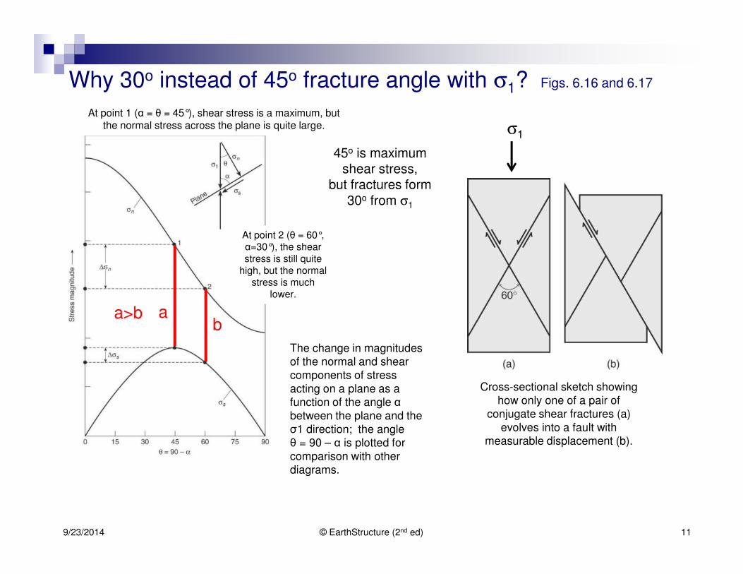
The change in magnitudes of the normal and shear components of stress acting on a plane as a function of the angle α between the plane and the σ1 direction; the angle θ = 90 – α is plotted for comparison with other diagrams.

At point 2 (θ = 60°, α=30°), the shear stress is still quite

high, but the normal stress is much

lower.

At point 1 (α = θ = 45°), shear stress is a maximum, but the normal stress across the plane is quite large.

a>bb

a

σ1

Cross-sectional sketch showing how only one of a pair of

conjugate shear fractures (a) evolves into a fault with

measurable displacement (b).

45o is maximum shear stress,

but fractures form

30o from σ1

Shear failure criteria – 2 Fig. 6.18

Parabolic failure envelope:

steeper near tensile field and shallower at high σn

Therefore, the value of α (the

angle between fault and σ1)

is not constant (compare

2α1, 2α2, and 2α3).

Fracture angle varies around 30o

Mohr-Coulomb criterion


Mohr failure envelope.

Shear failure criteria - 3


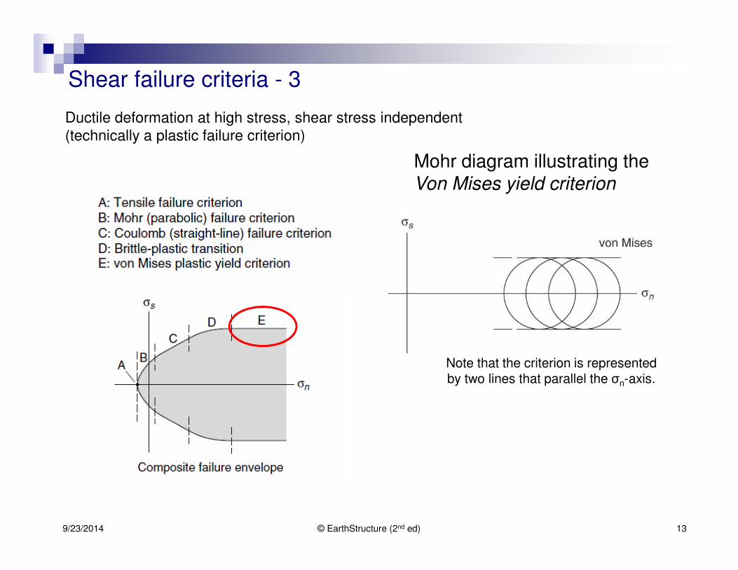
Ductile deformation at high stress, shear stress independent

(technically a plastic failure criterion)

Note that the criterion is represented by two lines that parallel the σn-axis.

Mohr diagram illustrating the Von Mises yield criterion

Composite Failure Envelope Fig. 6.21


A representative

composite failure

envelope on a Mohr

diagram.

Sketches of the fracture geometries that form during

failure. Note that the geometry depends on the part of the failure envelope

that represents failure conditions, because the

slope of the envelope is not constant.

Tensile crack: Griffith criterion

Shear fracture: Mohr-Coulomb criterion


Fault Types


Anderson’s Theory of Faulting

Faulting represents a response of rock to shear stress,

so it only occurs when the differential stress

(σd = σ1 – σ3 = 2σs) does not equal zero.

Because shear-stress magnitude on a plane changes

as a function of the orientation of the plane with

respect to the principal stresses, we should expect

a relationship between the orientation of faults

formed during a tectonic event and the trajectories

of principal stresses during that event.

Indeed, faults that initiate as Coulomb shear fractures

will form at an angle of about 30°to the σ1 direction

and contain the σ2 direction.

This relationship is called Anderson’s theory of

faulting.



σ1



• Recall the role of the normal stress, where the ratio of shear stress to normal stress on planes orientated at about 30°to σ1 is at a maximum. The Earth’s surface is a “free surface” (the contact between ground and air/fluid) that cannot, therefore, transmit a shear stress.

• Therefore, regional principal stresses are parallel or perpendicular to the surface of the Earth in the upper crust.

• Considering that gravitational body force is a major contributor to the stress state, and that this force acts vertically, stress trajectories in homogeneous, isotropic crust can maintain this geometry at depth.

states that in the Earth-surface reference

frame, normal faulting occurs where σ2 and σ3 are horizontal and σ1 is vertical, thrust

faulting occurs where σ1 and σ2 are horizontal and σ3 is vertical, and strike-slip faulting

occurs where σ1 and σ3 are horizontal and σ2 is vertical


• Moreover, the dip of thrust faults should be ∼30°, the dip of normal faults should be ∼60°, and the dip of strike-slip faults should be about vertical.

• For example, if the σ1 orientation at convergent margins is horizontal, Anderson’s theory predicts that thrust faults should form in this environment, and indeed belts of thrust faults form in collisional mountain belts.

• Anderson’s theory is a powerful tool for regional analysis, but we cannot use this theory to predict all fault geometries in the Earth’s crust for several reasons.

• First, faults do not necessarily initiate in intact rock.

• The frictional sliding strength of a preexisting surface is less than the shear failure strength of intact rock; thus, preexisting joint surfaces or faults may be reactivated before new faults initiate, even if the preexisting surfaces are not inclined at 30°to σ1 and do not contain the σ2 trajectory.

• Preexisting fractures that are not ideally oriented with respect to the principal stresses become oblique-slip faults.

Second, a fault surface is a material feature in a rock body whose orientation may change as the rock body containing the fault undergoes progressive deformation.

Thus, the fault may rotate into an orientation not predicted by Anderson’s theory

Frictional sliding


refers to movement on a surface that takes place when

shear stress parallel to surface exceeds frictional resistance to

sliding.

Amonton’s Laws of Friction:

•Frictional force is a function of normal

force.

•Frictional force is independent of

(apparent) area of contact.

•Frictional force is (mostly)

independent of material used.

(15th C da Vinci experiments)

The friction coefficients and, therefore, sliding forces (Ff) are equal for both objects, regardless of (apparent) contact area.

FIGURE 6.22 Frictional sliding of objects with same mass, but with different (apparent) contact areas.


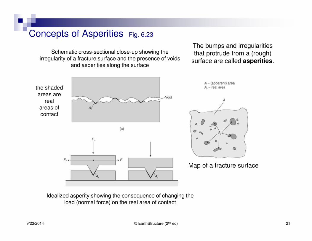
Concepts of Asperities Fig. 6.23

Real v. Apparent

Area of contact

Larger mass (F), deeperpenetration

Schematic cross-sectional close-up showing the irregularity of a fracture surface and the presence of voids

and asperities along the surface

Idealized asperity showing the consequence of changing the load (normal force) on the real area of contact

the shaded areas are

realareas of contact

Map of a fracture surface

The bumps and irregularities

that protrude from a (rough)

surface are called asperities.


Frictional Sliding Criteria (Byerlee’s Law) Fig. 6.24

Graph of shear stress and normal stress values

at the initiation of sliding on preexisting

fractures in a variety of rock types.

The best-fit line defines Byerlee’s

law, which is defined for two

regimes.

Byerlee’s Law depends on σn

For σn < 200 MPa, the best-fitting

criterion is σs = 0.85σn.

For 200 MPa <σn< 2000 MPa,

the best-fitting criterion is

σs = 50 MPa + 0.6σn.

coefficient of friction (µ)µ)µ)µ) is

a constant = σσσσs / σσσσn

µ = 0.6-0.85 (~0.7)


Sliding or Fracturing? Fig. 6.25

• Mohr diagram based on experiments with Blair dolomite, showing how a single stress

state (Mohr circle) would contact the frictional sliding envelope before it would contact

the Coulomb envelope (heavy line).

• Sliding occurs on surfaces between intersections with the friction envelope (marked by

shaded area for friction envelope µ = 0.85) before new fracture initiation.

Surface A in (b) is the Coulomb shear fracture that would form in an intact rock.

Preexisting surfaces B to E are surfaces that will slide with decreasing friction coefficients.

• Consider the geologic relevance of decreasing friction coefficients for stress state,

failure, and fracture orientation.coefficient of friction (µ) is constant = σs / σn


Effects of Fluids on Tensile Crack Growth Fig. 2.26

Hydrostatic (fluid) pressure

Pf = ρ ⋅ g ⋅ h, where ρ is density of water (1000 kg/m3), g is gravitational

constant (9.8 m/s2), and h is depth

Lithostatic pressure Pl = ρ ⋅ g ⋅ h, weight of overlying column

of rock (ρ = 2500–3000 kg/m3).

Graph of lithostatic versus hydrostatic pressure

as a function of depth in the Earth’s crust.

Fluid Pressure and Effective Stress


“outward push”

Mohr diagram showing how an increase

in pore pressure moves the Mohr circle

toward the origin.

σs = C + µ (σn – Pf) [fracturing]

σs = µ (σn – Pf) [sliding]

The increase in pore pressure decreases the mean stress (σmean), but does not change the magnitude

of differential stress (σ1 – σ3)

In other words, the diameter of the Mohr

circle remains constant, but its center moves to the

left.

Hydraulic fracturing

coefficient of friction (µ) is constant = σs / σn

(σn – Pf) is commonly labeled σn, the effective stress.

So, µeffective = µ (1 – Pf /σn)

µeffective ≤ µ

Slip and Earthquakes Looking ahead Fig. 8.36


Seismic slip (earthquake)

Aseismic slip (creep)

stress build-up then partial stress

release (“stress drop”).

Note: Stress drop is 1-10 MPa,

i.e. 1/10th of stress state !

stress drop

Laboratory frictional sliding experiment on

granite, showing stick-slip behavior. • The stress drops (dashed lines)

correspond to slip events.

• Associated microfracturing

activity is also indicated.

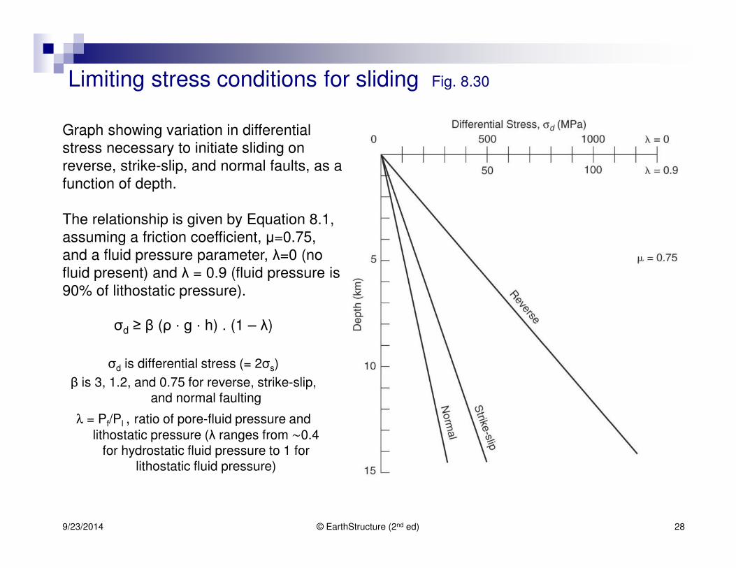
Limiting stress conditions for sliding Fig. 8.30

σd ≥ β (ρ ⋅ g ⋅ h) . (1 – λ)

σd is differential stress (= 2σs)

β is 3, 1.2, and 0.75 for reverse, strike-slip, and normal faulting

λ = Pf/Pl , ratio of pore-fluid pressure and

lithostatic pressure (λ ranges from ∼0.4 for hydrostatic fluid pressure to 1 for

lithostatic fluid pressure)


Graph showing variation in differential

stress necessary to initiate sliding on

reverse, strike-slip, and normal faults, as a

function of depth.

The relationship is given by Equation 8.1,

assuming a friction coefficient, µ=0.75,

and a fluid pressure parameter, λ=0 (no

fluid present) and λ = 0.9 (fluid pressure is

90% of lithostatic pressure).

Rate and Friction State


Lecture 6 Brittle Deformation - · PDF fileBrittle deformation is the permanent change that...

Documents

Transcript of Lecture 6 Brittle Deformation - · PDF fileBrittle deformation is the permanent change that...