Lecture 5 Short-Term Selection Response R = h 2 S.

Lecture 5Short-Term Selection

Response

R = h2 S

Applications of Artificial Selection

• Applications in agriculture and forestry • Creation of model systems of human diseases

and disorders• Construction of genetically divergent lines for

QTL mapping and gene expression (microarray) analysis

• Inferences about numbers of loci, effects and frequencies

• Evolutionary inferences: correlated characters, effects on fitness, long-term response, effect of mutations

Response to Selection

• Selection can change the distribution of phenotypes, and we typically measure this by changes in mean– This is a within-generation change

• Selection can also change the distribution of breeding values– This is the response to selection, the change

in the trait in the next generation (the between-generation change)

The Selection Differential and the Response to Selection

• The selection differential S measures the within-generation change in the mean– S = * -

• The response R is the between-generation change in the mean– R(t) = (t+1) - (t)

S

o

*p

R

( ) A Parental Generation

( ) B Offspring Generation

Truncation selection uppermost fraction

p chosen

Within-generationchange

Between-generationchange

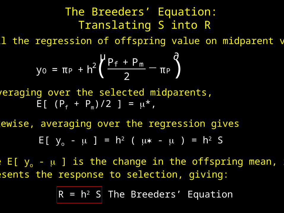
The Breeders’ Equation: Translating S into R

µ ∂yO = πP + h2 P f + Pm

2πP( )

Recall the regression of offspring value on midparent value

Averaging over the selected midparents, E[ (Pf + Pm)/2 ] = *,

E[ yo - ] = h2 ( - ) = h2 S

Likewise, averaging over the regression gives

Since E[ yo - ] is the change in the offspring mean, it represents the response to selection, giving:

R = h2 S The Breeders’ Equation

• Note that no matter how strong S, if h2 is small, the response is small

• S is a measure of selection, R the actual response. One can get lots of selection but no response

• If offspring are asexual clones of their parents, the breeders’ equation becomes – R = H2 S

• If males and females subjected to differing amounts of selection,– S = (Sf + Sm)/2– An Example: Selection on seed number in plants -- pollination

(males) is random, so that S = Sf/2

Response over multiple generations

• Strictly speaking, the breeders’ equation only holds for predicting a single generation of response from an unselected base population

• Practically speaking, the breeders’ equation is usually pretty good for 5-10 generations

• The validity for an initial h2 predicting response over several generations depends on:– The reliability of the initial h2 estimate– Absence of environmental change between

generations– The absence of genetic change between the

generation in which h2 was estimated and the generation in which selection is applied

(A)

S S

(B)

(C)

S

50% selectedVp = 4, S = 1.6



The selection differential is a function of boththe phenotypic variance and the fraction selected

The Selection Intensity, i

As the previous example shows, populations with thesame selection differential (S) may experience verydifferent amounts of selection

The selection intensity i provides a suitable measurefor comparisons between populations,

i =S

pVP

=S

æp

Selection Differential Under

Truncation Selection

E[z j z > T ] =Z 1

t

zp(z)ºT

dz = π +æ¢pT

ºT

Mean of truncated distribution

Height of the unit normal density functionat the truncation point T

P ( z > T)

Phenotypic standard deviationsHence, S = pT/ T

Likewise, i = S/ = pT/ T µ ∂ni ' 0:8+0:41 l

1p

° 1( )

pT = ¡∑T ° π

æ

∏

( )

Selection Intensity Versions of the Breeders’ Equation

R = h2S = h2 Sæp

æp = i h2æp

We can also write this as Since h2P = (2A/2

P) P = A(A/P) h A

R = i h A

Since h = correlation between phenotypic and breedingvalues, h = rPA

R = i rPAA

Response = Intensity * Accuracy * spread in Va

When we select an individual solely on their phenotype,the accuracy (correlation) between BV and phenotype is h

Accuracy of selectionMore generally, we can express the breedersequation as

R = i ruAA

Where we select individuals based on the index u(for example, the mean of n of their sibs).

ruA = the accuracy of using the measure u topredict an individual's breeding value = correlation between u and an individual's BV, A

Example: Estimating an individual’s BV withprogeny testing. For n progeny, ruA

2 = n/(n+a), where a = (4-h2)/h2

Overlapping Generations

Ry =im + if

Lm + Lf

h2p

Lx = Generation interval for sex x = Average age of parents when progeny are born

The yearly rate of response is

Trade-offs: Generation interval vs. selection intensity:If younger animals are used (decreasing L), i is also lower,as more of the newborn animals are needed as replacements

Generalized Breeder’s Equation

Ry =im + if

Lm + Lf

ruAA

Tradeoff between generation length L and accuracy r

The longer we wait to replace an individual, the moreaccurate the selection (i.e., we have time for progenytesting and using the values of its relatives)

Permanent Versus Transient Response

Considering epistasis and shared environmental values,the single-generation response follows from the midparent-offspring regression

R = h2 S +S

æ2z

µæ2

A A

2+

æ2A A A

4+¢¢¢+æ(Esi re;Eo) +æ(Edam;Eo)

∂

( )Breeder’s Equation

Response from epistasisResponse from shared environmental effects

Permanent component of responseTransient component of response --- contributesto short-term response. Decays away to zeroover the long-term

Response with Epistasis

R = Sµ

h2 +æ2

AA

2æ2z

∂

( )

R(1+ø) = Sµ

h2 +(1 ° c)ø æ2AA

2æ2z

∂

( )

The response after one generation of selection froman unselected base population with A x A epistasis is

The contribution to response from this single generationafter generations of no selection is

c is the average (pairwise) recombination between lociinvolved in A x A

Contribution to response from epistasis decays to zero aslinkage disequilibrium decays to zero

Response from additive effects (h2 S) is due to changes in allele frequencies and hence is permanent. Contribution from A x A due to linkage disequilibrium

R(t+ø) = th2 S + (1 ° c)ø RAA(t)

Why unselected base population? If history of previousselection, linkage disequilibrium may be present andthe mean can change as the disequilibrium decays

More generally, for t generation of selection followed by generations of no selection (but recombination)

Maternal Effects:Falconer’s dilution model

z = G + m zdam + e

Direct genetic effect on characterG = A + D + I. E[A] = (Asire + Adam)/2

Maternal effect passed from dam to offspring is justA fraction m of the dam’s phenotypic value

m can be negative --- results in the potential for a reversed response

The presence of the maternal effects means that responseis not necessarily linear and time lags can occur in response

Parent-offspring regression under the dilution model

In terms of parental breeding values,

E(zo j Adam; Asire;zdam) =Adam

2+

Asire

2+mzdam

Regression of BV on phenotype

A = πA +bAz (z ° πz ) +e

With no maternal effects, baz = h2

æA;M =mæ2A=(2 ° m)

With maternal effects, a covariance between BV and maternal effect arises, withThe resulting slope becomes bAz = h2 2/(2-m)

¢πz = Sdam

µh2

2 ° m+m

∂+ Ssire

h2

2 ° m

The response thus becomes

( )

109876543210

-0.15

-0.10

-0.05

0.00

0.05

0.10

Generation

Cu

mu

lati

ve R

esp

onse

to

Sel

ecti

on

(i

n t

erm

s of

S)

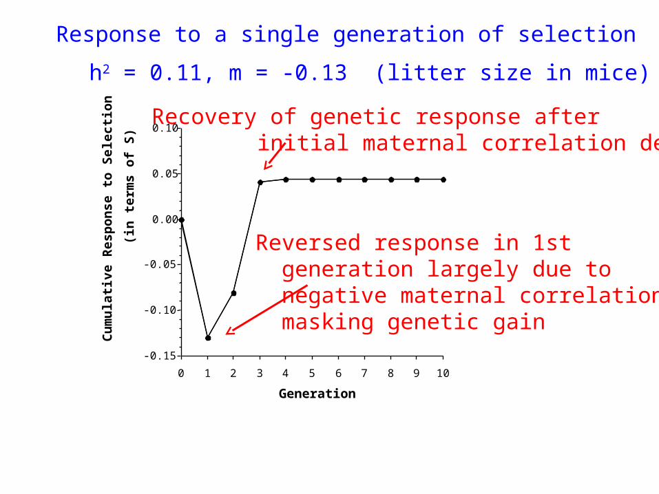
Response to a single generation of selection

Reversed response in 1st generation largely due to negative maternal correlation masking genetic gain

Recovery of genetic response after initial maternal correlation decays

h2 = 0.11, m = -0.13 (litter size in mice)

20151050

-1.0

-0.5

0.0

0.5

1.0

1.5

Generation

Cu

mu

lati

ve R

esp

onse

(in

un

its

of S

)

m = -0.25

m = -0.5

m = -0.75

h2 = 0.35

Selection occurs for 10 generations and then stops

Gene frequency changes under selection

Genotype A1A1 A1A2 A2A2

Fitnesses 1 1+s 1+2sAdditive fitnesses

Let q = freq(A2). The change in q from onegeneration of selection is:

¢q =sq(1 ° q)1+2sq

' sq(1 ° q) when j2sq j <<1

In finite population, genetic drift can overpowerselection. In particular, when 4Ne js j <<1drift overpowers the effects of selection

Strength of selection on a QTL


Contribution toCharacter

0 a 2a

Have to translate from the effects on a trait under selection to fitnesses on an underlying locus (or QTL)

Suppose the contributions to the trait are additive:

For a trait under selection (with intensity i) andphenotypic variance P

2, the induced fitnessesare additive with s = i (a / P )

Thus, drift overpowersselection on the QTL when 4Nejs j =

4Neja i jæP

<<1

More generally


Contribution to trait

0 a(1+k) 2a

Fitness 1 1+s(1+h) 1+2s

¢q ' 2q(1 ° q)[1+h(1 ° 2q)]

Change in allele frequency:

s = i (a / P )

Selection coefficients for a QTL

h = k

Changes in the Variance under Selection

The infinitesimal model --- each locus has a very smalleffect on the trait.

Under the infinitesimal, require many generations for significant change in allele frequencies

However, can have significant change in geneticvariances due to selection creating linkage disequilibrium

Under linkage equilibrium, freq(AB gamete) = freq(A)freq(B)

With positive linkage disequilibrium, f(AB) > f(A)f(B), so that AB gametes are more frequentWith negative linkage disequilibrium, f(AB) < f(A)f(B), so that AB gametes are less frequent

±æ2z =æ2

z °æ2z*

VA(1) = Va +d

Changes in VA with disequilibrium

Under the infinitesimal model, disequilibrium onlychanges the additive variance.Starting from an unselected base population, a single generation of selection generates a disequilibriumcontribution d to the additive variance

Additive genetic variance afterone generation of selection

Additive genetic variance in theunselected base population. Oftencalled the additive genic variance

disequilibrium

Changes in VA changes the phenotypic variance

Changes in VA and VP change the heritability

Within-generation changein the varianceA decrease in the variance

generates d < 0 and hencenegative disequilibrium

An increase in the variancegenerates d > 0 and hencepositive disequilibrium

d =æ2O °æ2

P =h4

2±æ2

z

The amount disequilibrium generated by a single generation of selection is

h2(1) =VA(1)VP (1)

=Va +dVP +d

VP (1) =VA(1) +VD +VE = VP +d

A “Breeders’ Equation” for Changes in Variance

d(0) = 0 (starting with an unselected base population)

d(t +1) =d(t)2

+h4(t)

2±æz(t)

Decay in previous disequilibrium from recombinationNew disequilibrium generated byselection that is passed onto thenext generation

d(t+1) =d(t)2

° kh4(t)

2æ2

z(t)

k > 0. Within-generationreduction in variance.negative disequilibrium, d < 0

k < 0. Within-generationincrease in variance.positive disequilibrium, d > 0

d(t+1) - d(t) measures the response in selectionon the variance (akin to R measuring the mean)

Within-generationchange in the variance-- akin to S

æ2z (t) = (1 ° k)æ2

z(t)

Many forms of selection (e.g., truncation) satisfyh2(t) =

VA (t)VP (t)

=Va +d(t)VP +d(t)

Lecture 5 Short-Term Selection Response R = h 2 S.

Documents

Transcript of Lecture 5 Short-Term Selection Response R = h 2 S.