Lecture 40 Sorting Techniques II

8/3/2019 Lecture 40 Sorting Techniques II

http://slidepdf.com/reader/full/lecture-40-sorting-techniques-ii 1/33

SortingTechniques



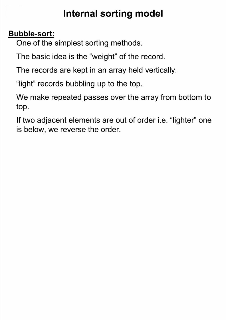
Bubble-sort:

One of the simplest sorting methods.

The basic idea is the ³weight´ of the record.

The records are kept in an array held vertically.

³light´ records bubbling up to the top.

We make repeated passes over the array from bottom to

top.

If two adjacent elements are out of order i.e. ³lighter´ oneis below, we reverse the order.

Internal sorting modelInternal sorting model



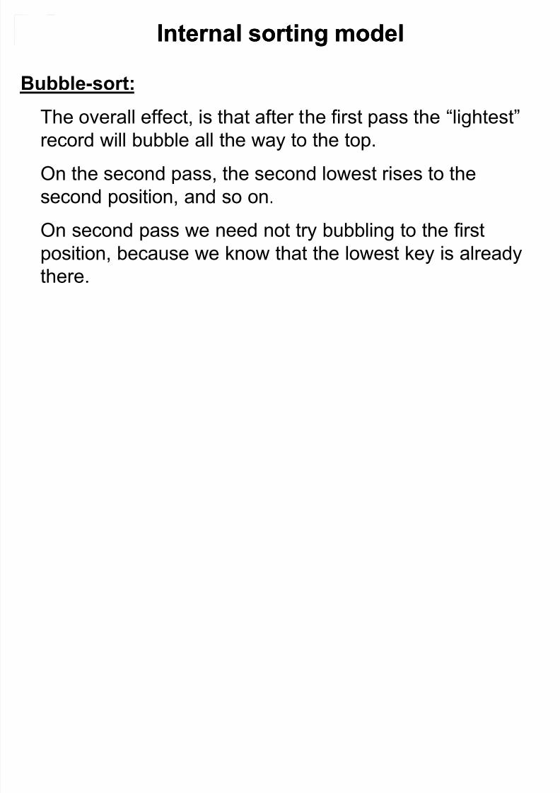
Bubble-sort:

The overall effect, is that after the first pass the ³lightest´

record will bubble all the way to the top.

On the second pass, the second lowest rises to the

second position, and so on.

On second pass we need not try bubbling to the first

position, because we know that the lowest key is already

there.




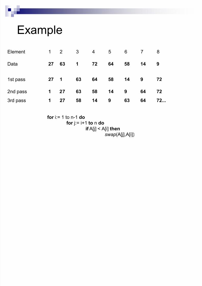
Example

Element 1 2 3 4 5 6 7 8

Data 27 63 1 72 64 58 14 9

1st pass 27 1 63 64 58 14 9 72

2nd pass 1 27 63 58 14 9 64 72

3rd pass 1 27 58 14 9 63 64 72...

f or i:= 1 to n-1 do

f or j:= i+1 to n do

if A[j] < A[i] then

swap( A[j],A[i])



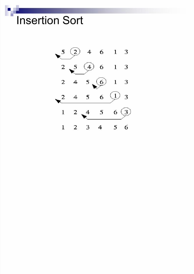
Insertion Sort

On the ith pass we ³insert´ the ith element A[i] into its rightful place

among A[1],A[2],«A[i-1] which were placed in sorted order.

After this insertion A[1],A[2],«A[i] are in sorted order.




Insertion SortA

1 n j

3 6 84 9 7 2 5 1

i

Strategy

Start ³empty handed´

Insert a card in the right

position of the already sortedhand

Continue until all cards are

inserted/sorted

for j=2 to length(A)

d o key=A[j]

³insert A[j] into the

sorted sequence A[1..j-1]´

i=j-1 while i>0 and A[i]>key

d o A[i+1]=A[i]

i--

A[i+1]:=key



Insertion Sort



Insertion Sort Time taken by Insertion Sort depends on

input: 1000 takes longer than 3 numbers

Can take different amounts of time to sort

2 input sequences of the same size

In general, the time taken by an algorithm

grows with the size of the input

Describe the running time of a program as

function of the size of input



Analysis of Algorithms Efficiency:

Running time

Space used

Efficiency as a function of input size:

Number of data elements (numbers, points)

A number of bits in an input number



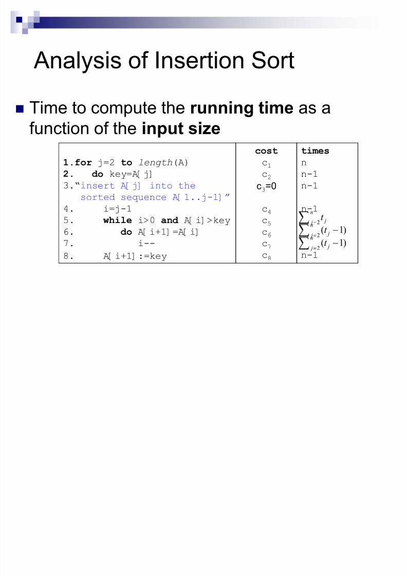
Analysis of Insertion Sort

1.for j=2 to length(A)

2. d o key=A[j]

3.³insert A[j] into the

sorted sequence A[1..j-1]´

4. i=j-1

5. while i>0 and A[i]>key

6. d o A[i+1]=A[i]

7. i--

8. A[i+1]:=key

cost

c1c2

c3=0

c4c5c6c7c8

times

n

n-1

n-1

n-1

n-1

2

n j jt

!§2( 1)

n

j jt

!§

2( 1)

n

j jt

!§

Time to compute the running time as a

function of the input size



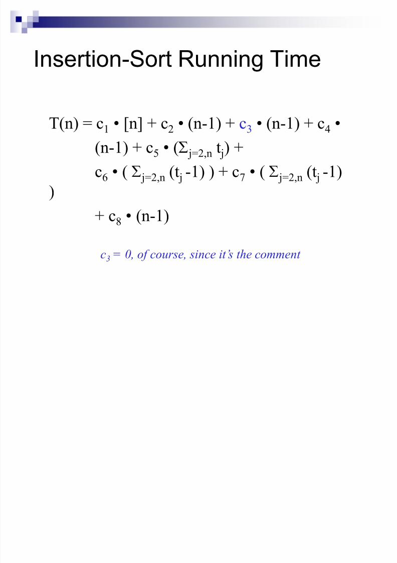
Insertion-Sort Running Time

T(n) = c1 [n] + c2 (n-1) + c3 (n-1) + c4

(n-1) + c5 (7 j=2,n t j) +

c6 ( 7 j=2,n (t j -1) ) + c7 ( 7 j=2,n (t j -1)

)

+ c8 (n-1)

c3 = 0, of course, since it¶ s the comment



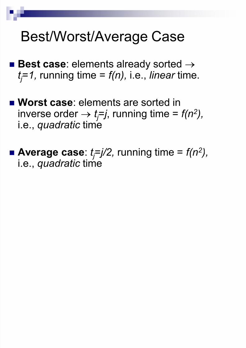
Best/Worst/Average Case Best case: elements already sortedp

t j =1, running time = f(n), i.e., li near time.

Worst case: elements are sorted ininverse order p t j =j , running time = f(n2 ),

i.e., quadratic time

Average case: t j =j/ 2 , running time = f(n2 ),i.e., quadratic time



Best Case Result

Occurs when array is already sorted.

For each j = 2, 3,«..n we find that A[i]<=key in line5 when I has its initial value of j-1.

T(n) =

c1 n + (c2 + c4) (n-1) + c5 (n-1)+ c8 (n-1)= n ( c1 + c2 + c4 + c5 + c8 )

+ ( -c2 ± c4 - c5 ± c8 )

= c9n + c10

= f 1(n1) + f 2(n

0)



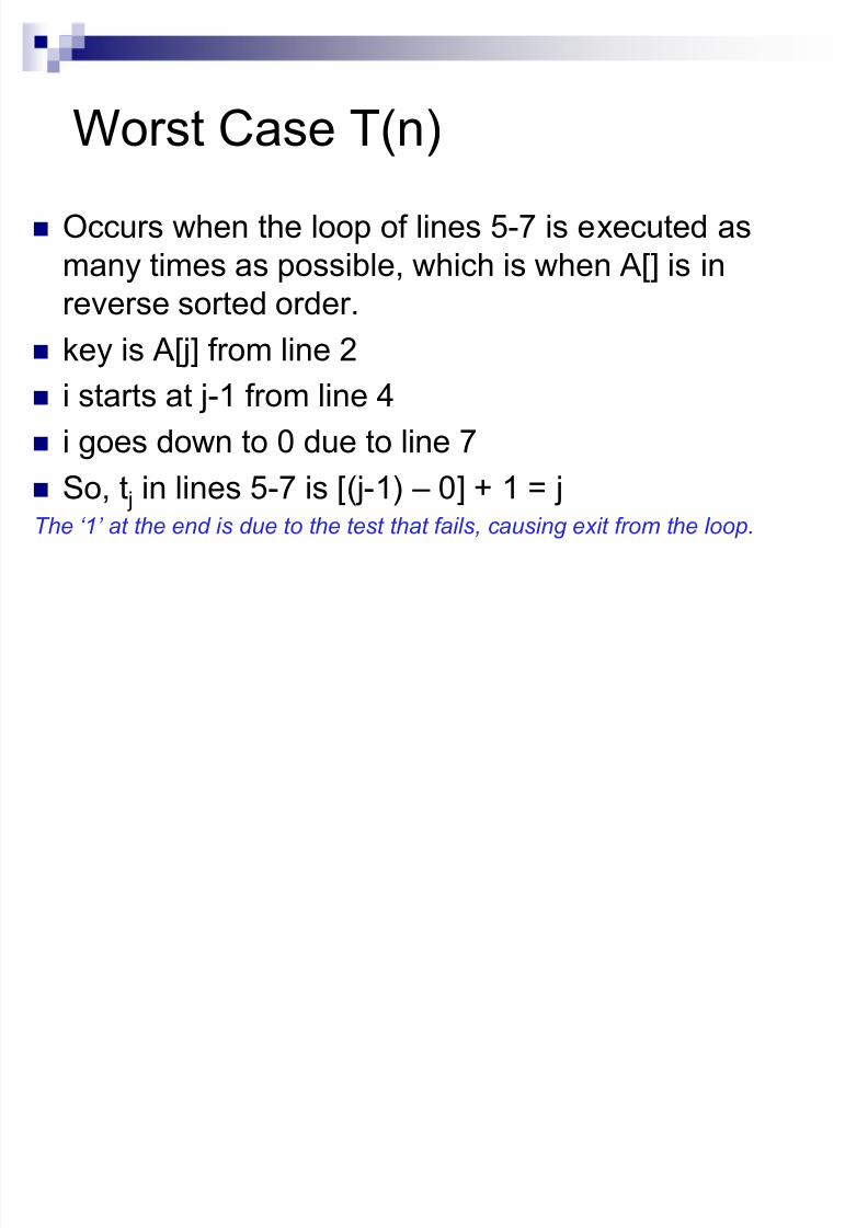
Worst Case T(n) Occurs when the loop of lines 5-7 is executed as

many times as possible, which is when A[] is in

reverse sorted order. key is A[j] from line 2

i starts at j-1 from line 4

i goes down to 0 due to line 7 So, t j in lines 5-7 is [( j-1) ± 0] + 1 = jThe µ1¶ at t he end i s d ue to t he t est t hat f ail s, c ausi ng ex it f r om t he loo p.



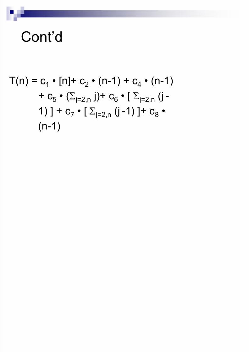
Cont¶d

T(n) = c1

[n]+ c2

(n-1) + c4

(n-1)

+ c5 (7 j=2,n j)+ c6 [ 7 j=2,n ( j -

1) ] + c7 [ 7 j=2,n ( j -1) ]+ c8

(n-1)



Cont¶d

T(n) =

c1 n + c2 (n-1) + c4 (n-1) + c8 (n-1)+ c5 (7 j=2,n j)

+ c6 [ 7 j=2,n ( j -1) ]+ c7 [ 7 j=2,n ( j -1) ]

= c9 n + c10 + c5 (7 j=2,n j) + c11

[7 j=2,n ( j -1) ]



Cont¶d

T(n) = c9 n + c10 + c5 (7 j=2,n j) + c11 [ 7 j=2,n ( j -1)]

But7 j=2,n j = [n(n+1)/2] ± 1

so that

7 j=2,n ( j-1) = 7 j=2,n j ± 7 j=2,n (1)

= [n(n+1)/2] ± 1 ± (n-2+1)= [n(n+1)/2] ± 1 ± n + 1 = n(n+1)/2 - n

= [n(n+1)-2n]/2 = [n(n+1-2)]/2 = n(n-1)/2



Cont¶d

In conclusion,

T(n) =c9 n + c10 + c5 [n(n+1)/2] ± 1 + c11 n(n-

1)/2

= c12 n2

+ c13 n + c14

= f 1(n2) + f 2(n

1) + f 3(n0)



Selection Sort Given an array of length n,

Search elements 0 through n-1 and select the smallest

Swap it with the element in location 0

Search elements 1 through n-1 and select the smallest Swap it with the element in location 1

Search elements 2 through n-1 and select the smallest

Swap it with the element in location 2

Search elements3

through n-1 and select the smallest Swap it with the element in location 3

Continue in this fashion until there¶s nothing left to

search



Example and analysis of Selection

Sort The Selection Sort might

swap an array element with

itself--this is harmless.

7 2 8 5 4

2 7 8 5 4

2 4 8 5 7

2 4 5 8 7

2 4 5 7 8



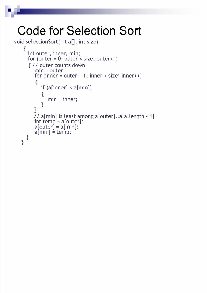
Code for Selection Sortvoid selectionSort(int a[], int size)

{int outer, inner, min;for (outer = 0; outer < size; outer++)

{ // outer counts down

min = outer;for (inner = outer + 1; inner < size; inner++)

{if (a[inner] < a[min])

{min = inner;

}

}// a[min] is least among a[outer]..a[a.length - 1]int temp = a[outer];a[outer] = a[min];a[min] = temp;

}

}



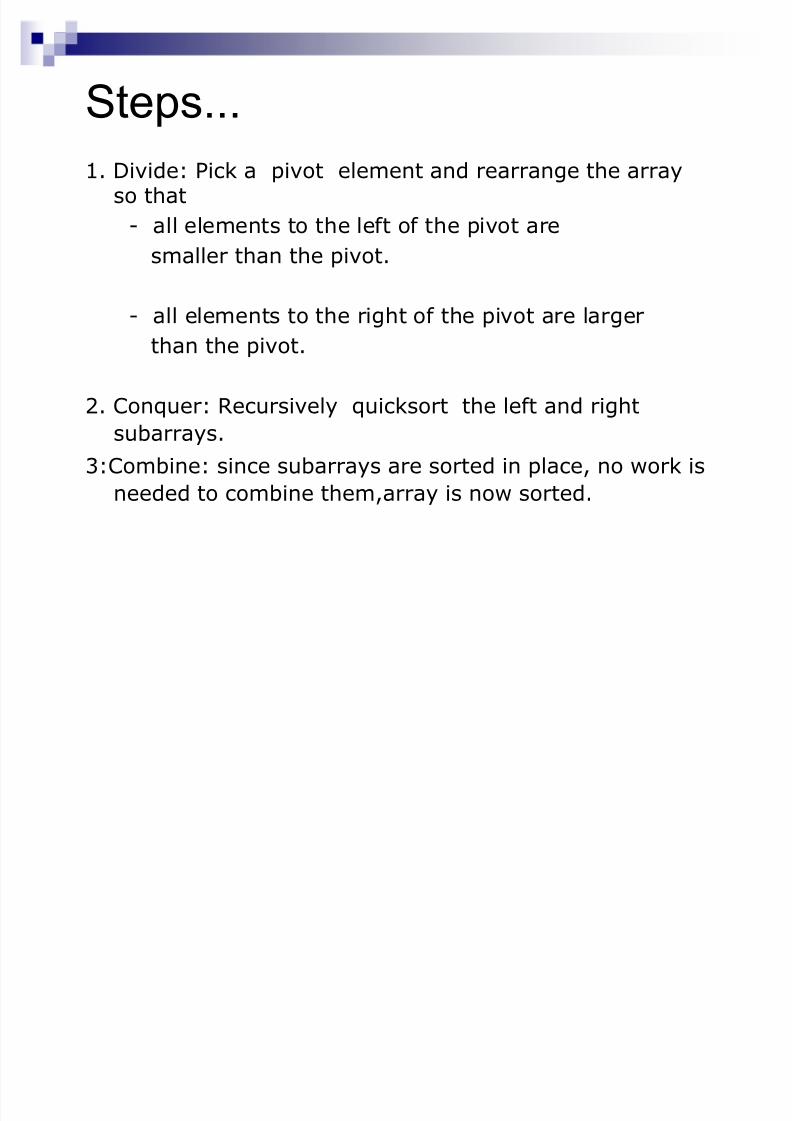
Quick Sort : Based on Divide and Conquer paradigm.

One of the fastest in-memory sorting algorithms (if not the fastest)

is a very efficient sorting algorithmdesigned by C.A.R.Hoare in 1960.

Consists of two phases:

Partition phaseSort phase

Quick Sort



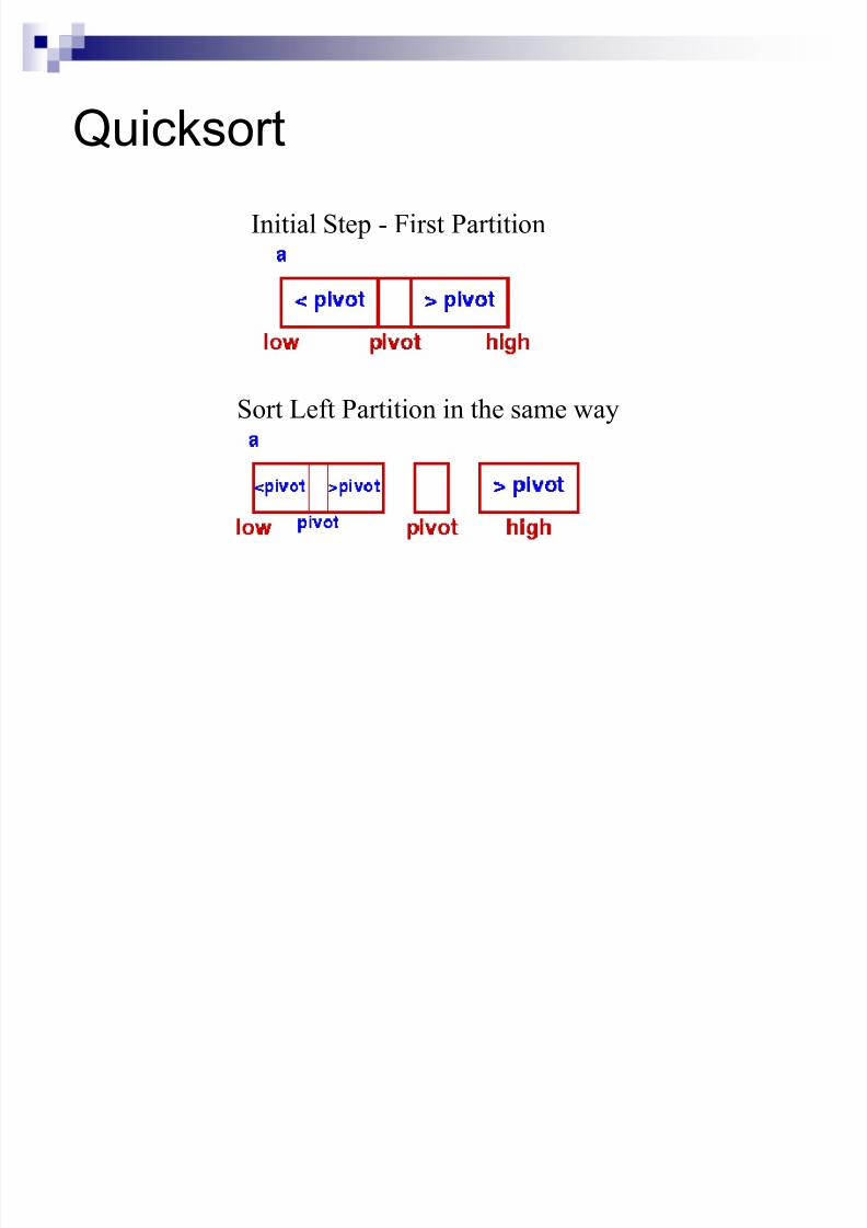
Quicksort

Sor t Left Par tition in the same way

Initial Step - Fir st Par tition



Quicksort ± Partition phase Goals:

Select pivot value

Move everything less than pivot value to the left of it Move everything greater than pivot value to the right

of it



Algorithm: Quick Sort

if ( r > l ) then j n partition ( A, l , r );QuickSort ( A, l , j - 1 );QuickSort ( A, j + 1 , r );

end of if.

Procedure QuickSort ( A, l , r )



9 8 2 3 88 34 5 10 11 0

5 8 2 3 0 9 34 11 10 88

Partition

l

r l j

r

A

A



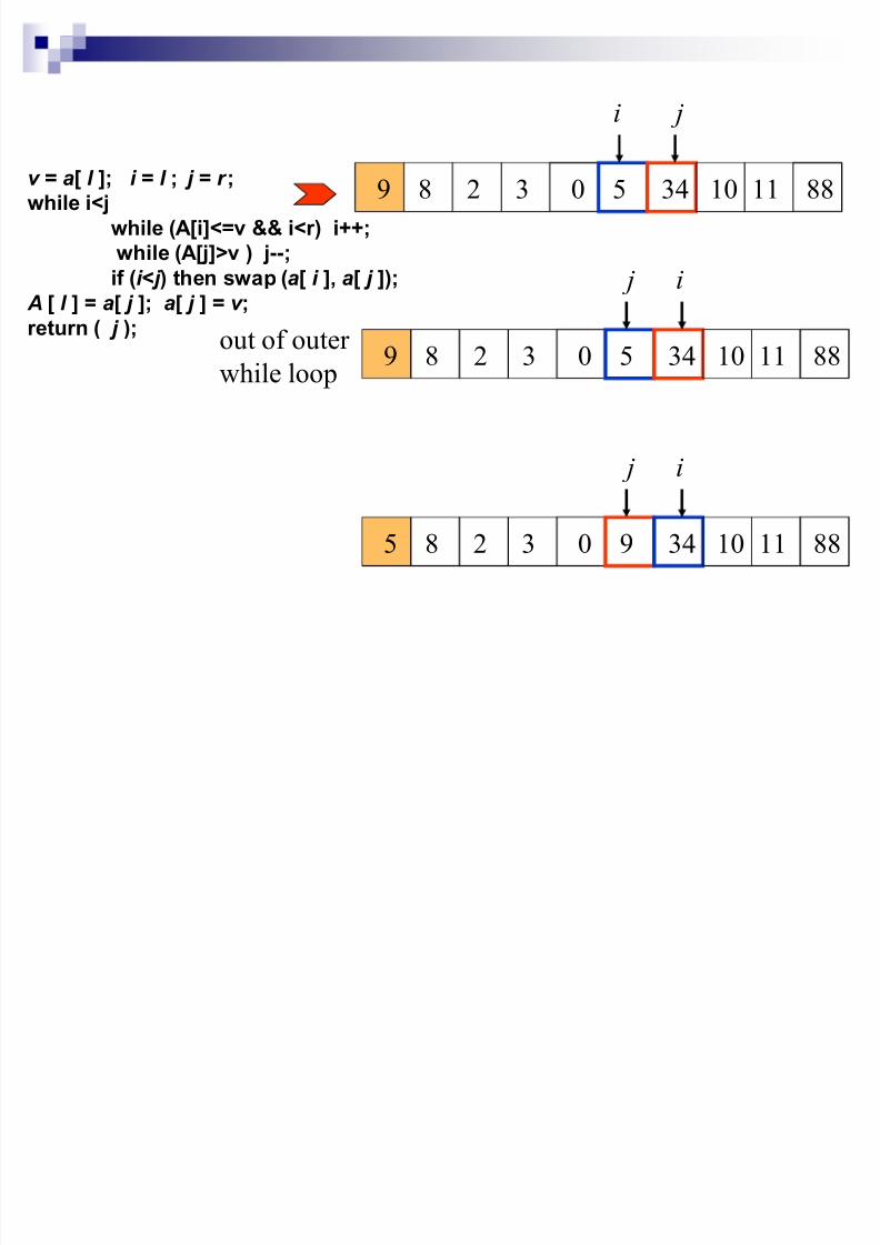
Algorithm: Partition

Function P artition ( A, l , r )

v n a[ l ]; i n l ; j n r ;

while i<jwhile (A[i]<=v && i<r) i++;while (A[ j]>v ) j--;if (i<j ) then swap (a[ i ], a[ j ]);

A [ l ] = a[ j ]; a[ j ] n v ;

return ( j );

There are various algorithms for partition.Above Algorithm is the most popular. This is because it doesnot need an extra array. Only 3 variables v ,i , and j.



9 8 2 3 88 34 5 10 11 0

i jv 9

9 8 2 3 88 34 5 10 11 0

i j

9 8 2 3 0 34 5 10 11 88

i j

9 8 2 3 0 34 5 10 11 88

i j

v = a[ l ]; i = l ; j = r ;

while i<j

while (A[i]<=v && i<r) i++;

while (A[j]>v ) j--;

if (i<j ) then swap (a[ i ], a[ j ]);

A [ l ] = a[ j ]; a[ j ] = v ;

return ( j );



9 8 2 3 0 5 34 10 11 88

i j

9 8 2 3 0 5 34 10 11 88

i j

5 8 2 3 0 9 34 10 11 88

i j

out of outer

while loo p

v = a[ l ]; i = l ; j = r ;

while i<j

while (A[i]<=v && i<r) i++;

while (A[j]>v ) j--;

if (i<j ) then swap (a[ i ], a[ j ]);

A [ l ]=

a[ j ]; a[ j ]=

v ;return ( j );



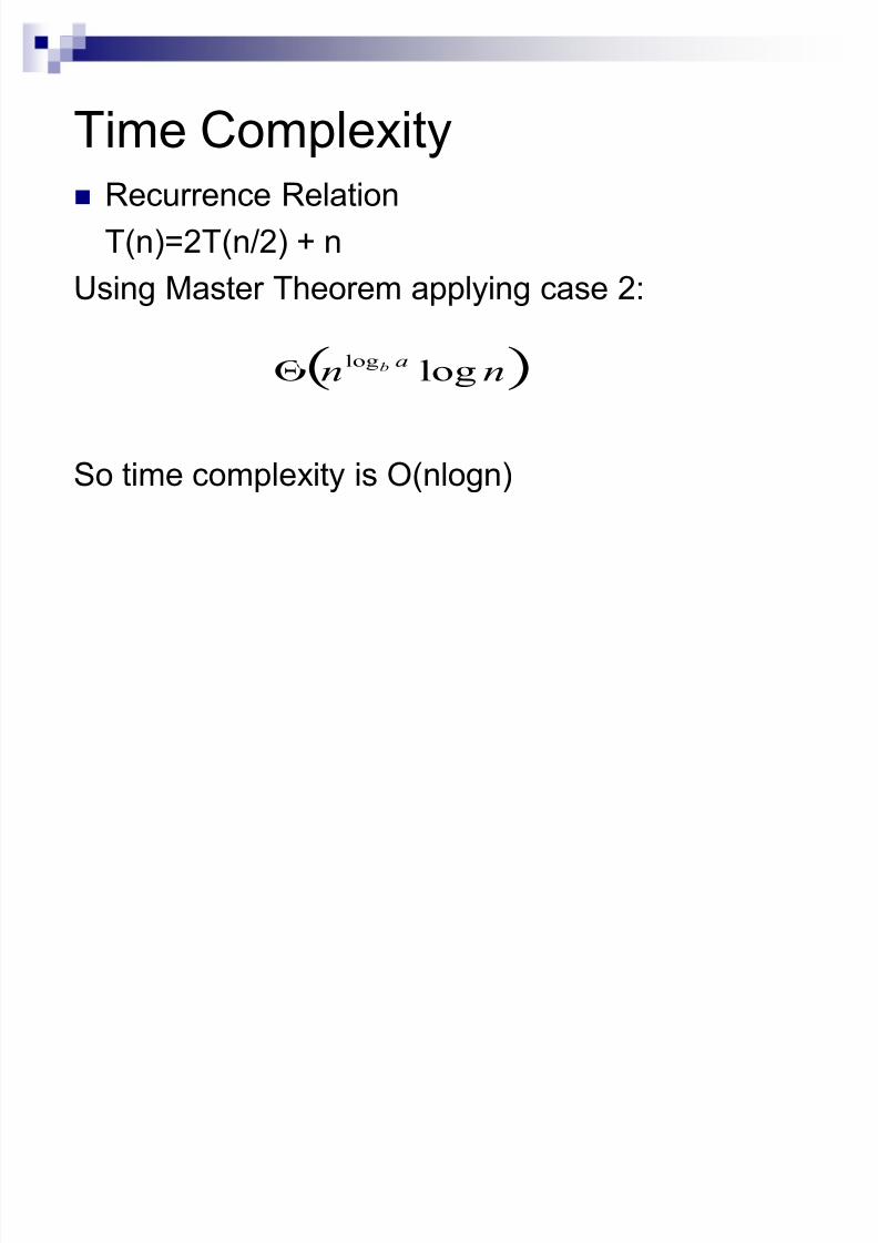
Time Complexity Recurrence Relation

T(n)=2T(n/2) + n

Using Master Theorem applying case 2:

So time complexity is O(nlogn)

nna

b loglog

5



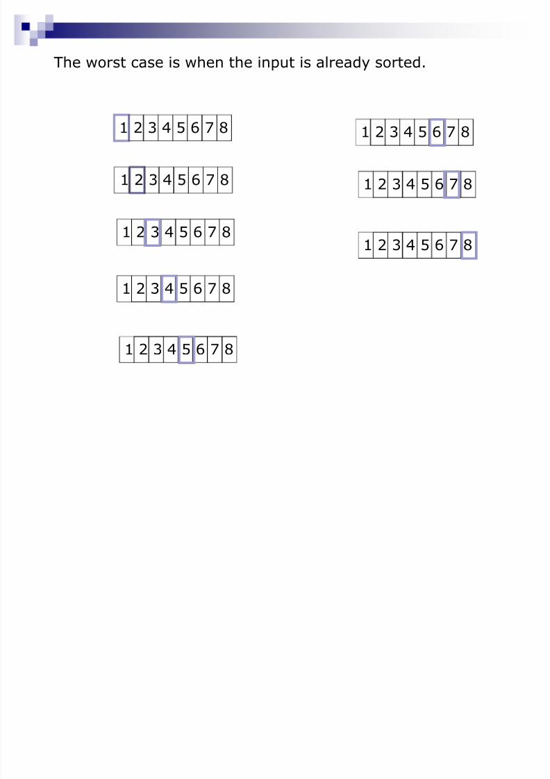
The worst case is when the input is already sorted.

1 2 3 4 5 6 7 8

1 2 3 4 5 6 7 8

1 2 3 4 5 6 7 8

1 2 3 4 5 6 7 8

1 2 3 4 5 6 7 8

1 2 3 4 5 6 7 8

1 2 3 4 5 6 7 8

1 2 3 4 5 6 7 8



Randomized Quick Sort

Randomize the input data before giving it to QuickSort. OR

In the partition phase, rather than choosing firstvalue to be the pivot value, choose a RANDOMvalue to be pivot value.

This makes Quick Sort run time independent of

input ordering So Worst case won¶t happen for SORTED inputs

but may only happen by worseness of randomnumber generator.

Lecture 40 Sorting Techniques II

Documents

Transcript of Lecture 40 Sorting Techniques II