Lecture 4 Visualization and Animation
25
1 Lecture 4 Visualization and Animation
Transcript of Lecture 4 Visualization and Animation

1
Lecture 4
Visualization and Animation
2
Use Mathematica to visualize
the motion of physical
systems
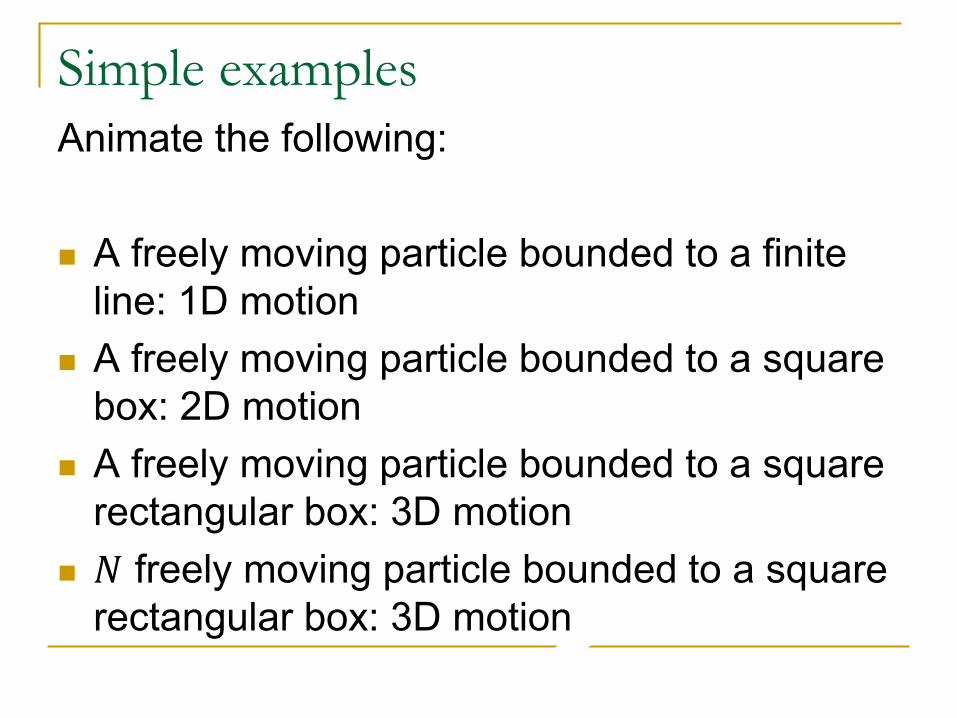
Simple examples
Animate the following:
A freely moving particle bounded to a finite
line: 1D motion
A freely moving particle bounded to a square
box: 2D motion
A freely moving particle bounded to a square
rectangular box: 3D motion
𝑁 freely moving particle bounded to a square
rectangular box: 3D motion
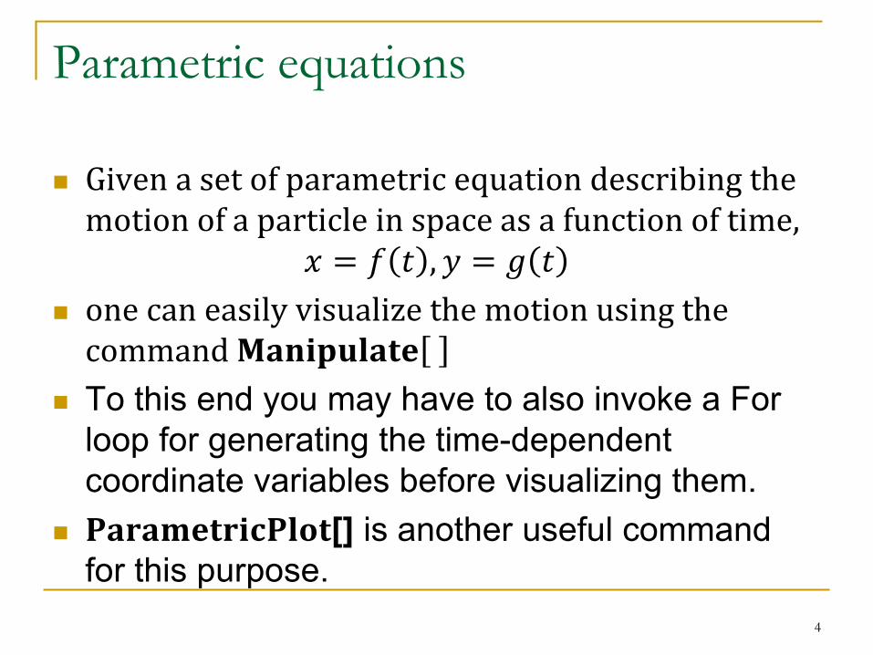
Parametric equations
Given a set of parametric equation describing the motion of a particle in space as a function of time,
𝑥 = 𝑓 𝑡 , 𝑦 = 𝑔 𝑡
one can easily visualize the motion using the command 𝐌𝐚𝐧𝐢𝐩𝐮𝐥𝐚𝐭𝐞
To this end you may have to also invoke a For
loop for generating the time-dependent
coordinate variables before visualizing them.
𝐏𝐚𝐫𝐚𝐦𝐞𝐭𝐫𝐢𝐜𝐏𝐥𝐨𝐭[] is another useful command
for this purpose.
4
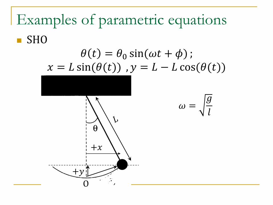
Examples of parametric equations
SHO𝜃 𝑡 = 𝜃0 sin(𝜔𝑡 + 𝜙) ;
𝑥 = 𝐿 sin(𝜃(𝑡)) , 𝑦 = 𝐿 − 𝐿 cos(𝜃(𝑡))
O
+𝑥
𝜔 =𝑔
𝑙
+𝑦
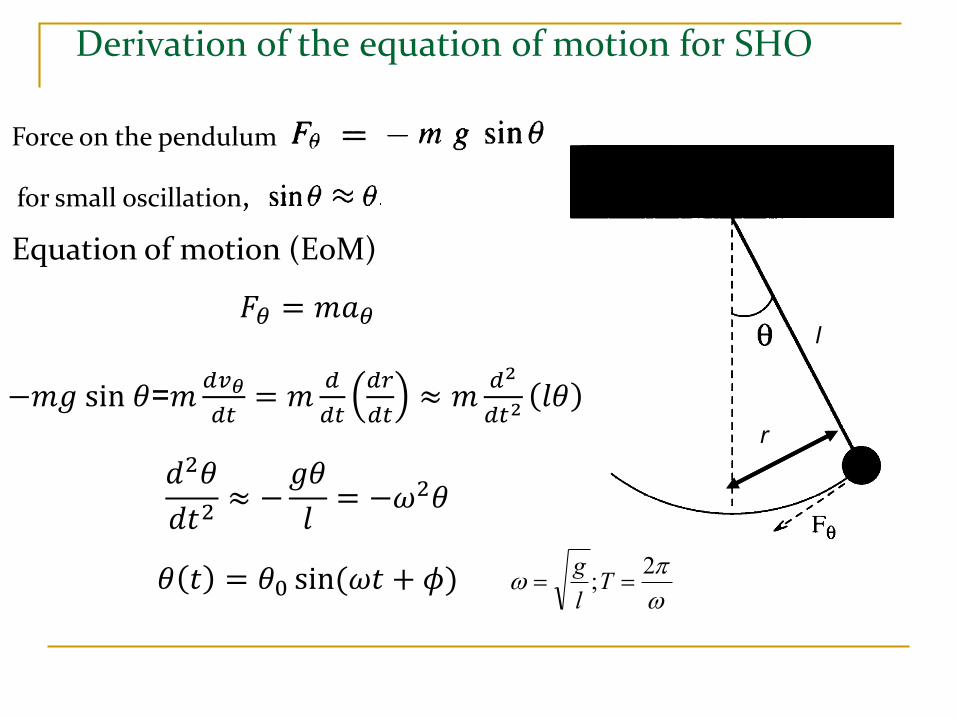
Derivation of the equation of motion for SHO
Equation of motion (EoM)
Force on the pendulum
2; Tl
g
for small oscillation,
𝐹𝜃 = 𝑚𝑎𝜃
−𝑚𝑔 sin 𝜃=𝑚𝑑𝑣𝜃
𝑑𝑡= 𝑚
𝑑
𝑑𝑡
𝑑𝑟
𝑑𝑡≈ 𝑚
𝑑2
𝑑𝑡2𝑙𝜃
𝑑2𝜃
𝑑𝑡2≈ −
𝑔𝜃
𝑙= −𝜔2𝜃
𝜃 𝑡 = 𝜃0 sin(𝜔𝑡 + 𝜙)
r
l
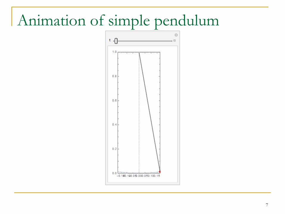
Animation of simple pendulum
7
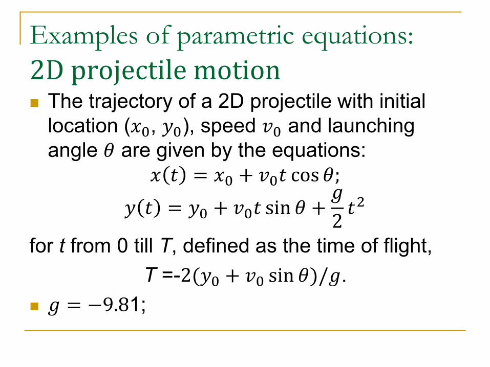
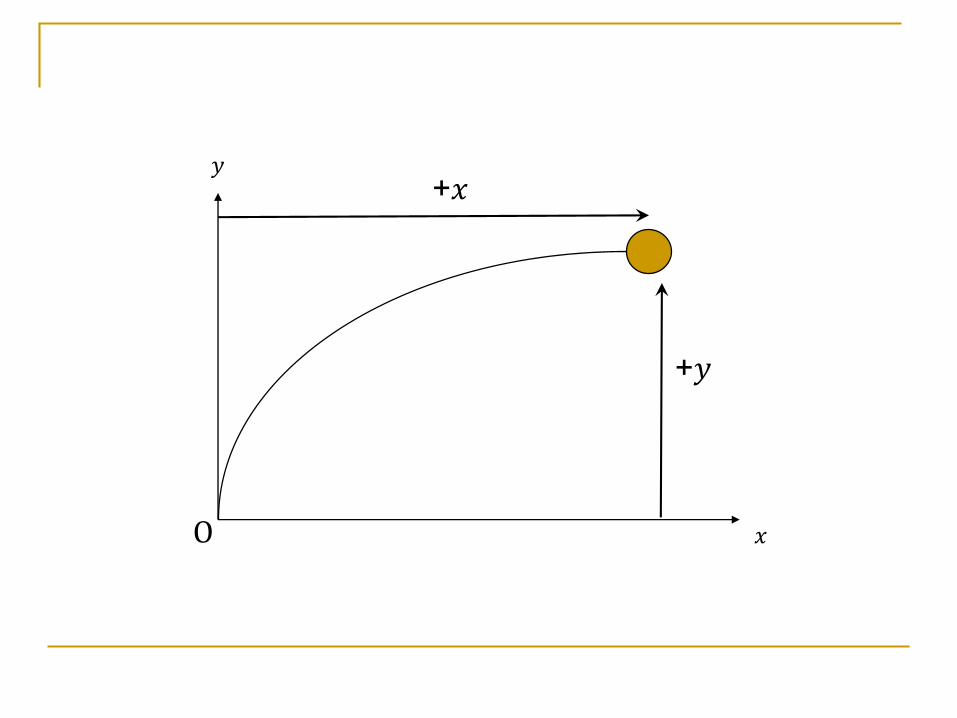
Examples of parametric equations:
2D projectile motion The trajectory of a 2D projectile with initial
location (𝑥0, 𝑦0), speed 𝑣0 and launching
angle 𝜃 are given by the equations:
𝑥 𝑡 = 𝑥0 + 𝑣0𝑡 cos 𝜃;
𝑦 𝑡 = 𝑦0 + 𝑣0𝑡 sin 𝜃 +𝑔
2𝑡2
for t from 0 till T, defined as the time of flight,
T =-2(𝑦0 + 𝑣0 sin 𝜃)/𝑔.
𝑔 = −9.81;
𝑥
𝑦+𝑥
+𝑦
O
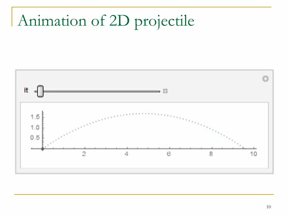
Animation of 2D projectile
10
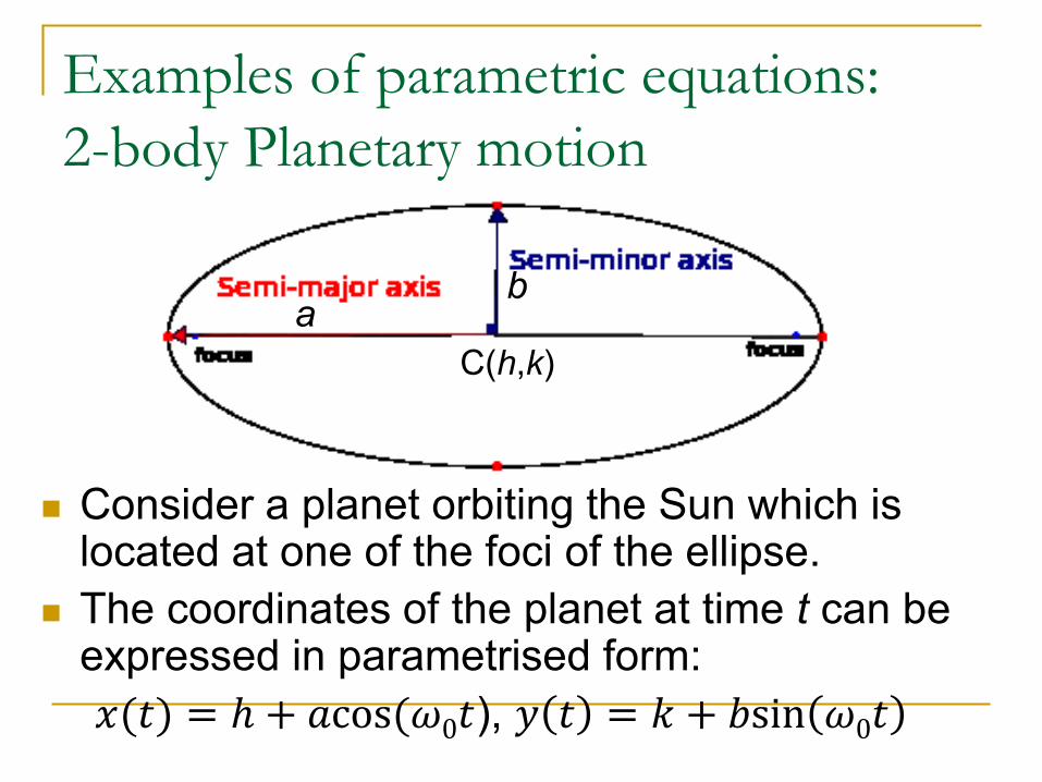
Consider a planet orbiting the Sun which islocated at one of the foci of the ellipse.
The coordinates of the planet at time t can be expressed in parametrised form:
𝑥(𝑡) = ℎ + 𝑎cos(𝜔0𝑡), 𝑦 𝑡 = 𝑘 + 𝑏sin 𝜔0𝑡
Examples of parametric equations:
2-body Planetary motion
C(h,k)
ba
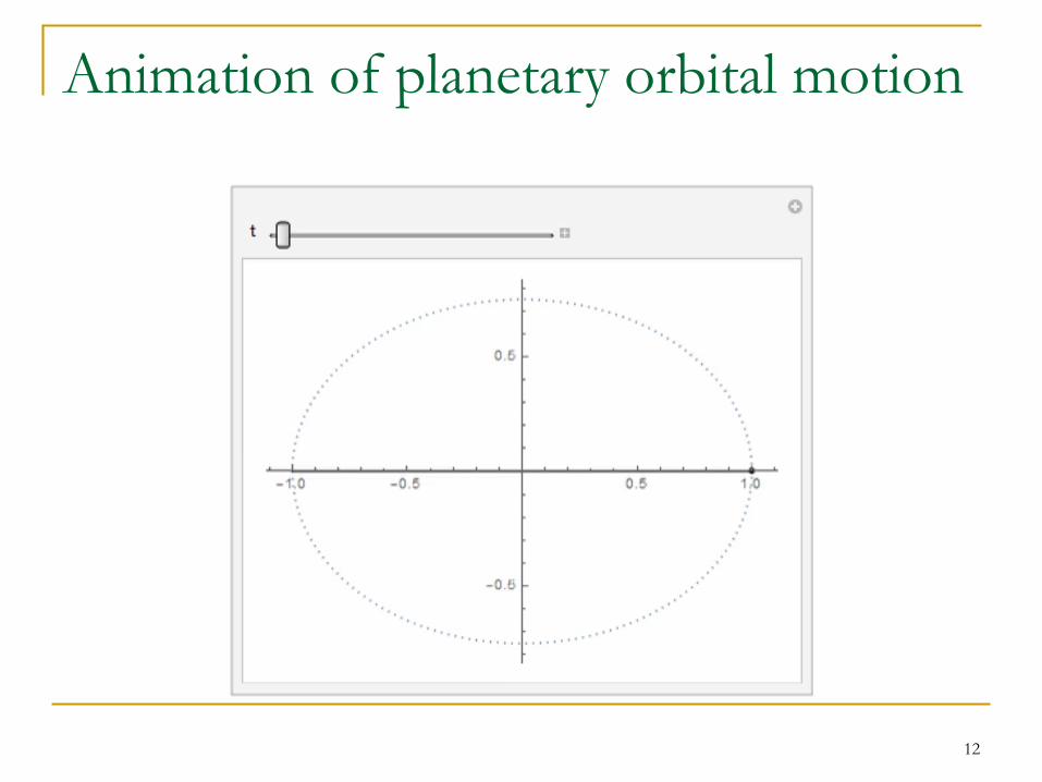
Animation of planetary orbital motion
12

Assignments
By using the corresponding parametric
equations for the (𝑥, 𝑦) coordinates,
1. Animate a SHO (w/o drag force and driving
force)
2. Animate 2D projectile motion (w/o drag force
and driving force)
3. Animate 2-body planetary motion
1D sinusoidal wave A sinusoidal wave is fundamentally
characterized by two quantities: wave number (equivalent to wave length) and angular frequency (frequency)
𝑘𝑥, 𝜔 or 𝜆, 𝑓 .
Wave number 𝑘𝑥 =2𝜋
𝜆; 𝜆 wave length
Angular frequency 𝜔 = 2𝜋𝑓; 𝑓 frequency
14
1D sinusoidal wave 𝜓 𝑥, 𝑡 = 𝐴 sin 𝜃(𝑥, 𝑡) ;
𝜃 𝑥, 𝑡 = 𝑘𝑥𝑥 − 𝜔𝑡 + 𝜙
Phase velocity of the wave can be obtained by
imposing the condition:𝜕𝜃(𝑥, 𝑡)
𝜕𝑡= 0
⇒ 𝑘𝑥𝜕𝑥
𝜕𝑡− 𝜔 = 0
⇒ 𝑣𝑥 =𝜕𝑥
𝜕𝑡=
𝜔
𝑘𝑥= 𝑓𝜆
𝑣𝑥 =𝜔
𝑘𝑥implies the wave is moving to the +𝑥
direction. 15
1D sinusoidal wave
If 𝜓 𝑥, 𝑡 = 𝐴 sin 𝜃(𝑥, 𝑡) , with
𝜃 𝑥, 𝑡 = 𝑘𝑥𝑥 + 𝜔𝑡 + 𝜙,
⇒ 𝑣𝑥 = −𝜔
𝑘𝑥
This wave is moving to the -𝑥 direction.
16
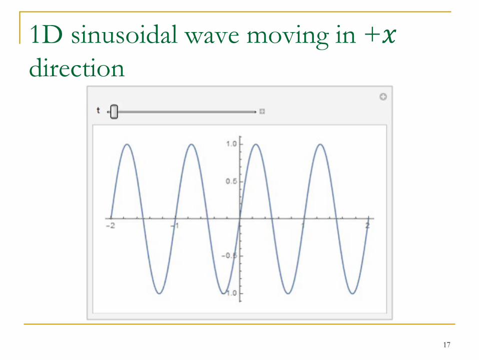
1D sinusoidal wave moving in +𝑥direction
17
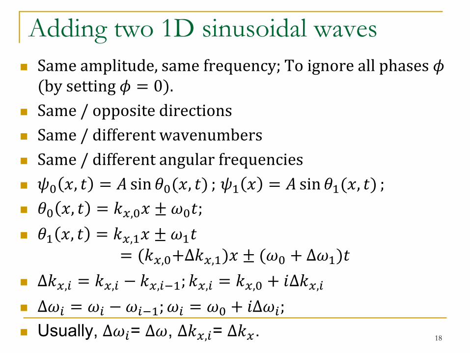
Adding two 1D sinusoidal waves
Same amplitude, same frequency; To ignore all phases 𝜙(by setting 𝜙 = 0).
Same / opposite directions
Same / different wavenumbers
Same / different angular frequencies
𝜓0 𝑥, 𝑡 = 𝐴 sin 𝜃0(𝑥, 𝑡) ; 𝜓1 𝑥 = 𝐴 sin 𝜃1(𝑥, 𝑡) ;
𝜃0 𝑥, 𝑡 = 𝑘𝑥,0𝑥 ± 𝜔0𝑡;
𝜃1 𝑥, 𝑡 = 𝑘𝑥,1𝑥 ± 𝜔1𝑡= (𝑘𝑥,0+Δ𝑘𝑥,1)𝑥 ± (𝜔0 + Δ𝜔1)𝑡
Δ𝑘𝑥,𝑖 = 𝑘𝑥,𝑖 − 𝑘𝑥,𝑖−1; 𝑘𝑥,𝑖 = 𝑘𝑥,0 + 𝑖Δ𝑘𝑥,𝑖
Δ𝜔𝑖 = 𝜔𝑖 −𝜔𝑖−1; 𝜔𝑖 = 𝜔0 + 𝑖Δ𝜔𝑖;
Usually, Δ𝜔𝑖= Δ𝜔, Δ𝑘𝑥,𝑖= Δ𝑘𝑥.18
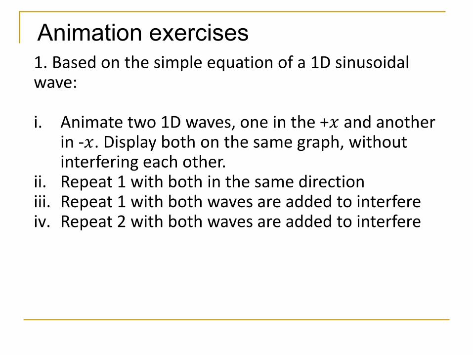
Animation exercises1. Based on the simple equation of a 1D sinusoidal wave:
i. Animate two 1D waves, one in the +𝑥 and another in -𝑥. Display both on the same graph, without interfering each other.
ii. Repeat 1 with both in the same directioniii. Repeat 1 with both waves are added to interfereiv. Repeat 2 with both waves are added to interfere
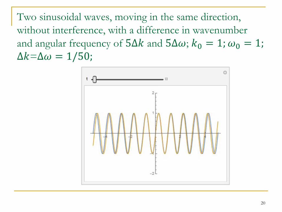
Two sinusoidal waves, moving in the same direction,
without interference, with a difference in wavenumber
and angular frequency of 5Δ𝑘 and 5Δ𝜔; 𝑘0 = 1;𝜔0 = 1;Δ𝑘=Δ𝜔 = 1/50;
20
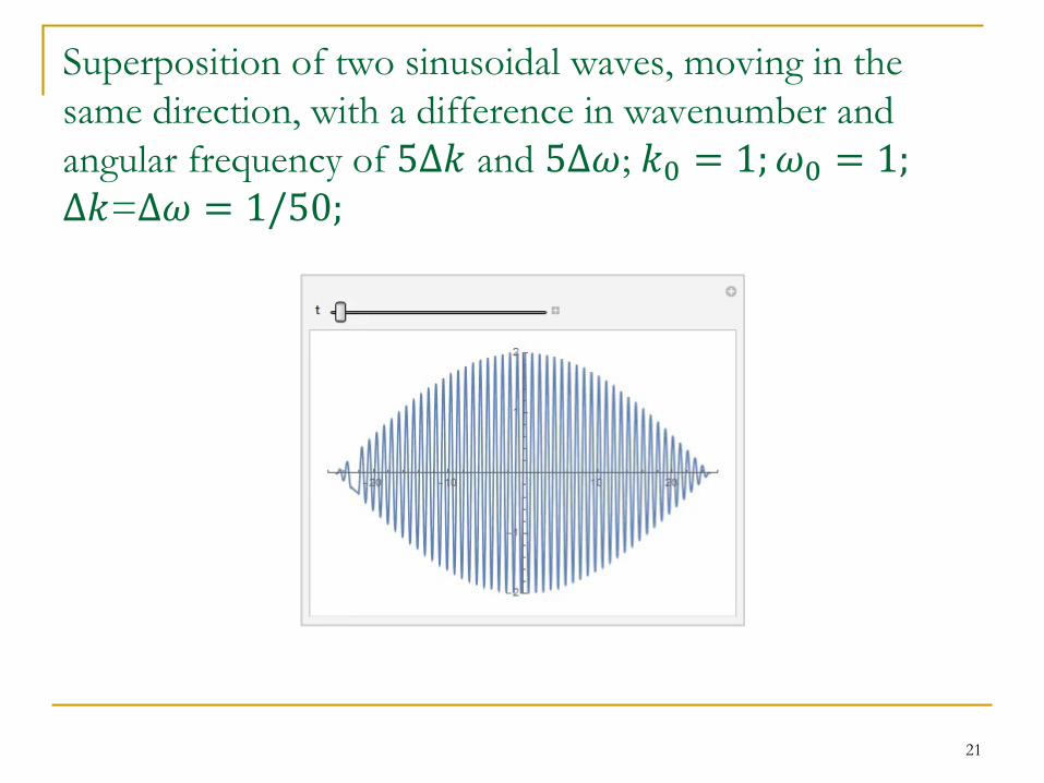
Superposition of two sinusoidal waves, moving in the
same direction, with a difference in wavenumber and
angular frequency of 5Δ𝑘 and 5Δ𝜔; 𝑘0 = 1;𝜔0 = 1;Δ𝑘=Δ𝜔 = 1/50;
21
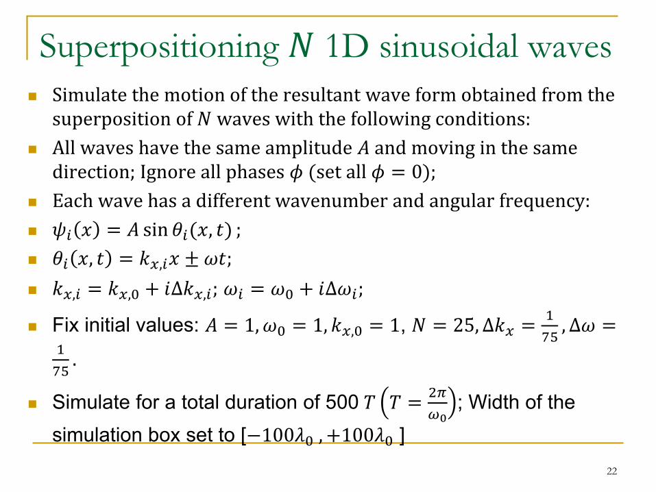
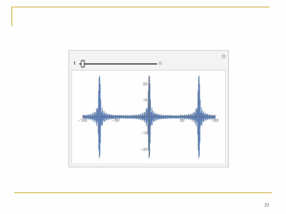
Superpositioning 𝑁 1D sinusoidal waves
Simulate the motion of the resultant wave form obtained from the superposition of 𝑁 waves with the following conditions:
All waves have the same amplitude 𝐴 and moving in the same direction; Ignore all phases 𝜙 (set all 𝜙 = 0);
Each wave has a different wavenumber and angular frequency:
𝜓𝑖 𝑥 = 𝐴 sin 𝜃𝑖(𝑥, 𝑡) ;
𝜃𝑖 𝑥, 𝑡 = 𝑘𝑥,𝑖𝑥 ± 𝜔𝑡;
𝑘𝑥,𝑖 = 𝑘𝑥,0 + 𝑖Δ𝑘𝑥,𝑖; 𝜔𝑖 = 𝜔0 + 𝑖Δ𝜔𝑖;
Fix initial values: 𝐴 = 1,𝜔0 = 1, 𝑘𝑥,0 = 1, 𝑁 = 25, Δ𝑘𝑥 =1
75, Δ𝜔 =
1
75.
Simulate for a total duration of 500 𝑇 𝑇 =2𝜋
𝜔0; Width of the
simulation box set to [−100𝜆0 , +100𝜆0 ]
22
23
Animation exercises1. Animate an outgoing 2D sinusoidal wave
2. Animate two outgoing 2D sinusoidal waves from two different origins that display interference.

More complicated examples
Damped, forced SHO
2D projectile motion with drag force from the
air
Three-body planetary motion
25