Lecture 4 — Symmetry in the solid state -Part IV: Brillouin zones and the symmetry of the band

structure.

1 Symmetry in Reciprocal Space — the Wigner-Seitz construc-tion and the Brillouin zones

Non-periodic phenomena in the crystal (elastic or inelastic) are described in terms ofgeneric (non-RL) reciprocal-space vectors and give rise to scattering outside theRL nodes.

In describing these phenomena, however, one encounters a problem: as one moves away from theRL origin, symmetry-related “portions” of reciprocal space will become very distant from eachother. In order to take full advantage of the reciprocal-space symmetry, it is therefore advanta-geous to bring symmetry-related parts of the reciprocal space together in a compact form.This is exactly what the Wigner-Seitz (W-S) constructions accomplish very cleverly. ”Brillouinzones” is the name that is given to the portions of the extended W-S contructions that are “broughtback together”. A very good description of the Wigner-Seitz and Brillouin constructions can befound in [3].

1.1 The Wigner-Seitz construction

The W-S construction is essentially a method to construct, for every Bravais lattice, a fully-symmetric unit cell that has the same volume of a primitive cell. As such, it can be applied toboth real and reciprocal spaces, but it is essentially employed only for the latter.

For a given lattice node τ , the W-S unit cell containing τ is the set of points that are closerto τ than to any other lattice node.

It is quite apparent that:

• Each W-S unit cell contains one and only one lattice node.

• Every point in space belongs to at least one W-S unit cell. Points belonging to more than onecell are boundary points between cells.

• From the previous two points, it is clear that the W-S unit cell has the same volume of aprimitive unit cell. In fact, it “tiles” the whole space completely with identical cells, eachcontaining only one lattice node.

1

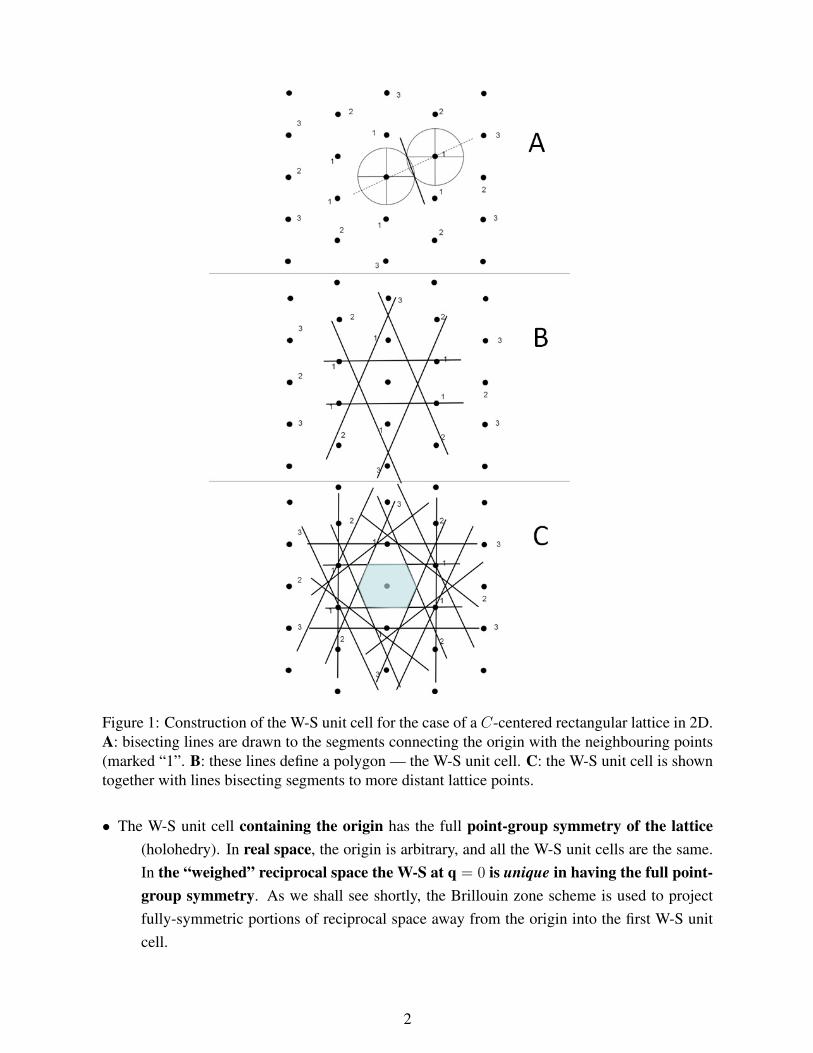
Figure 1: Construction of the W-S unit cell for the case of a C-centered rectangular lattice in 2D.A: bisecting lines are drawn to the segments connecting the origin with the neighbouring points(marked “1”. B: these lines define a polygon — the W-S unit cell. C: the W-S unit cell is showntogether with lines bisecting segments to more distant lattice points.

• The W-S unit cell containing the origin has the full point-group symmetry of the lattice(holohedry). In real space, the origin is arbitrary, and all the W-S unit cells are the same.In the “weighed” reciprocal space the W-S at q = 0 is unique in having the full point-group symmetry. As we shall see shortly, the Brillouin zone scheme is used to projectfully-symmetric portions of reciprocal space away from the origin into the first W-S unitcell.

2

A dummies’ guide to the W-S construction (fig. 1)

• Draw segments connecting the origin with the neighbouring points. The first “ring” of points(marked with “1” in fig. 1 A) should be sufficient, although these points may not all besymmetry-equivalent.

• Draw orthogonal lines bisecting the segments you just drew. These lines define a polygoncontaining the origin (fig. 1 B)— this is the W-S unit cell. In 3D, one would need to draworthogonal bisecting planes, yielding W-S polyhedra.

• Fig. 1 C shows an extended construction (to be used later) including lines bisecting thesegments to the second and third “rings”. As you can see, the new lines do not intersectthe original W-S unit cell.

• The whole space can be “tiled” with W-S cells (fig. 2).

1.1.1 “Reduction” to the first Wigner-Seitz unit cell (first Brillouin zone).

As anticipated, the main use of the W-S unit cell is in reciprocal space:

Every vector q in reciprocal space can be written as

q = k + τ (1)

where τ is a RL vector and k is within the first W-S unit cell. (i.e., the one containing theorigin). We more often say that k is the “equivalent” of q reduced to the first Brillouin zone(see here below).The repeated W-S scheme shown in fig. 2 is used to determine which τ should be used for agiven q — clearly, the one corresponding to the lattice node closer to it.

1.2 The extended W-S construction: higher Brillouin zones

We have just learned how to “reduce” every reciprocal-space point to the first W-S unit cell (orfirst Brillouin zone). But the question is: which “bits” of reciprocal space should be “reduced”together? One may be tempted to think that an entire W-S unit cell around a RL point should be“reduced” together — after all, one would only need a single RL vector to accomplish this. Itis readily seen, however, that this is not a good idea. As we mentioned before, higher W-S unitcells (i.e., other than the first) do not possess any symmetry, and we are specifically interestedin “reducing” together symmetry-related parts of reciprocal space. Therefore, a different con-struction, known as the extended W-S construction-is required to reduce symmetry-related

3

Figure 2: Repeated W-S cell scheme, showing how the entire space can be tiled with these cells.Each cell can be “reduced” to the first W-S cell with a single RL vector.

portions of reciprocal space simultaneously.

The first Brillouin zone coincides with the first W-S unit cell. Higher W-S unit cells areemphatically not Brilloun zones.

4

Figure 3: The extended W-S construction. The starting point is fig. 1 C. A A number is givento each polygon, according to how many lines are crossed to reach the origin. Polygons with thesame number belong to the same Brillouin zone. The figure shows the scheme for the first threeBrillouin zones. B Portions of a higher Brillouin zone can be reduced to the first Brillouin zonein the normal way, i.e., by using the repeated W-S construction (here, the reduction procedure isshown for the third zone). C When reduced, higher zones “tile” perfectly within the first W-Scell.

5

A dummies’ guide to the extended W-S construction (fig. 3)

• Start off in the same way as for the “normal” W-S construction, but with lines bisecting thesegments to higher-order “rings” of points, as per fig. 1 C.

• Many polygons of different shapes (polyhedra in 3D) will be obtained. Each of these will begiven a number according to how many lines (planes in 3D) are crossed to reach theorigin with a straight path. If m lines (planes) are crossed, the order of the Brillouinzone will be m+ 1.

• A Brillouin zone is formed by polygons (polyhedra) having the same number (fig. 3 A).

• As anticipated, the first Brillouin zone is also the first W-S cell (no line is crossed).

• The different portions of a Brillouin zone are “reduced” to the first Brillouin zone in thenormal way, i.e., using the repeated W-S construction (fig. 3 B).

• All the portions of a higher Brillouin zone will tile perfectly within the first Brillouin zone(fig. 3 C).

2 Symmetry of the electronic band structure

We will now apply the concepts introduced here above to describe a number of important prop-erties of all wave-like excitations in crystals that can be determined purely based on symmetryconsiderations. We will only consider the case of electronic wavefunctions, but it is important tostate that almost identical considerations can be applied to other wave-like excitations in crystals,such as phonons and spin waves (magnons).

The starting point of this discussion is the Bloch theorem, which you have already encounteredin previous courses. Later in the course we will present a general symmetry prospective of thistheorem, but here we will just quote the main results: the electronic eigenstates of a Hamiltonianwith a periodic potential are of the Bloch form:

ψk(r) = eik·ruk(r) (2)

where uk(r) has the periodicity of the crystal. We also recall that the crystal wavevector k canbe limited to the first Brillouin zone (BZ). In fact, a function ψk′(r) = eik

′·ruk′(r) with k′ outsidethe first BZ can be rewritten as

ψk′(r) = eik·r[eiτ ·ruk′(r)

](3)

6

k  

Figure 4: A set of typical 1-dimensional electronic dispersion curves in the reduced/repeatedzone scheme.

where k′ = τ +k, k is within the 1st BZ and τ is a reciprocal lattice vector (RLV ). Note that thefunction in square brackets has the periodicity of the crystal, so that eq. 3 is in the Bloch form.

The application of the Bloch theorem to 1-dimensional (1D) electronic wavefunctions, usingeither the nearly-free electron approximation or the tight-binding approximation leads to thetypical set of electronic dispersion curves (E vs. k relations) shown in fig. 4. We draw attentionto three important features of these curves:

Properties of the electronic dispersions in 1D

• They are symmetrical (i.e., even) around the origin.

• The left and right zone boundary points differ by the RLV 2π/a, and are also related bysymmetry.

• The slope of the dispersions is zero both at the zone centre and at the zone boundary. Werecall that the slope (or more generally the gradient of the dispersion is related to thegroup velocity of the wavefunctions in band n by:

vn(k) =1

~∂En(k)

∂k(4)

7

As we shall see shortly, these 1D properties do not give much of a clue of what goes on in 2Dand 3D. We will just state the corresponding properties in 2D and 3D, and proceed to give somejustification of these statements.

Properties of the electronic dispersions in 2D and 3D

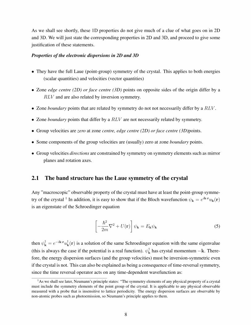
• They have the full Laue (point-group) symmetry of the crystal. This applies to both energies(scalar quantities) and velocities (vector quantities)

• Zone edge centre (2D) or face centre (3D) points on opposite sides of the origin differ by aRLV and are also related by inversion symmetry.

• Zone boundary points that are related by symmetry do not not necessarily differ by a RLV .

• Zone boundary points that differ by a RLV are not necessarily related by symmetry.

• Group velocities are zero at zone centre, edge centre (2D) or face centre (3D)points.

• Some components of the group velocities are (usually) zero at zone boundary points.

• Group velocities directions are constrained by symmetry on symmetry elements such as mirrorplanes and rotation axes.

2.1 The band structure has the Laue symmetry of the crystal

Any ”macroscopic” observable property of the crystal must have at least the point-group symme-try of the crystal 1 In addition, it is easy to show that if the Bloch wavefunction ψk = eik·ruk(r)

is an eigenstate of the Schroedinger equation

[− ~2

2m∇2 + U(r)

]ψk = Ekψk (5)

then ψ†k = e−ik·ru†k(r) is a solution of the same Schroedinger equation with the same eigenvalue

(this is always the case if the potential is a real function). ψ†k has crystal momentum −k. There-fore, the energy dispersion surfaces (and the group velocities) must be inversion-symmetric evenif the crystal is not. This can also be explained as being a consequence of time-reversal symmetry,since the time reversal operator acts on any time-dependent wavefunction as:

1As we shall see later, Neumann’s principle states: “The symmetry elements of any physical property of a crystalmust include the symmetry elements of the point group of the crystal. It is applicable to any physical observablemeasured with a probe that is insensitive to lattice periodicity. The energy dispersion surfaces are observable bynon-atomic probes such as photoemission, so Neumann’s principle applies to them.

8

Figure 5: (a)The Fermi surface of Sr2RuO4 (space group I4/mmm) from A. Damascelli et al.,Phys. Rev. Lett. 85, 5194 (2000) (ARPES experiment) and I. I. Mazin and D. J. Singh, Phys.Rev. Lett. 82, 4324 (1999), respectively. (b) The Fermi surface (top) and the band dispersion(bottom) of Bi2Te3 (space group R3̄m), as measured by ARPES by Y.L. Chen, J.G. Analytis,J.H. Chu, et al. Science 325, 178 (2009).

t→ −t, ψ(x, t)→ ψ∗(x,−t) (6)

The Laue symmetry of the electronic constant-energy surfaces, including of course the Fermisurface, can be seen beautifully using an experimental techniques called Angle-Resolved Pho-toemission Spectroscopy (ARPES). Very briefly, in ARPES the energy-momentum relations forelectrons in metals and semiconductors can be determined experimentally by illuminating a crys-tal with UV or soft-X-ray radiation of precisely known energy and direction and measuring theenergy and momentum of the photo-electrons ejected from the surface. Fig. 5 provides twographical illustration of ARPES data for crystals with different symmetries.

2.2 The group velocity is zero at zone-centre points and has additional con-straints at the zone boundary and on high-symmetry directions

The following conditions are a straightforward consequence of symmetry and the fact that veloc-ity is an ordinary (polar) vector.

• The group velocity at two points related by inversion in the BZ must be opposite.

• For points related by a mirror plane or a 2-fold axis, the components of the group velocityparallel and perpendicular to the plane or axis must be equal or opposite, respectively.

9

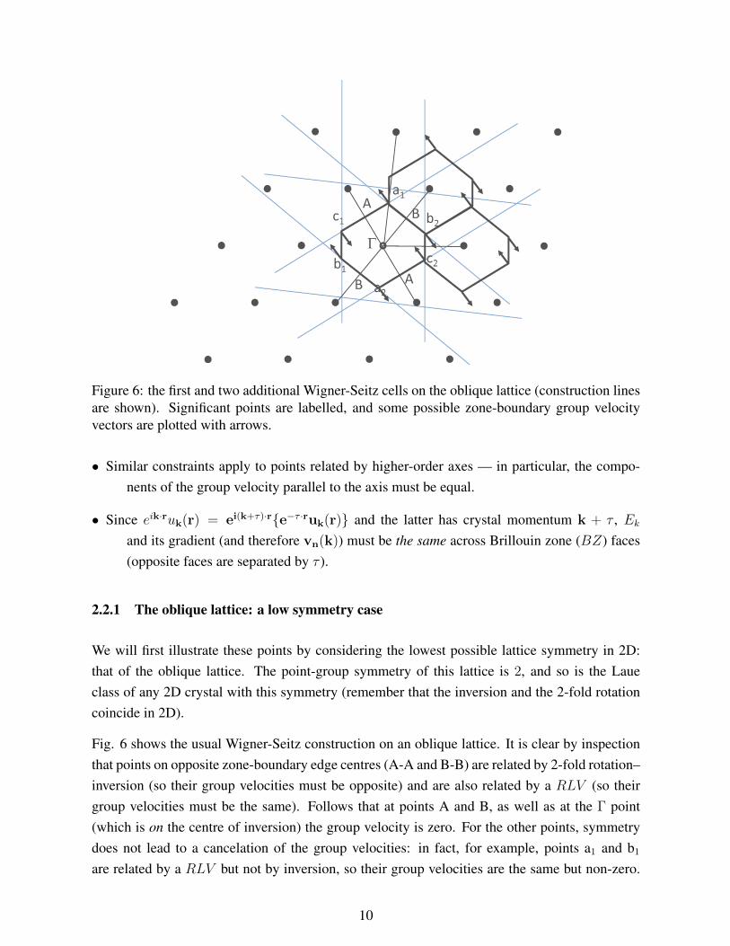
Figure 6: the first and two additional Wigner-Seitz cells on the oblique lattice (construction linesare shown). Significant points are labelled, and some possible zone-boundary group velocityvectors are plotted with arrows.

• Similar constraints apply to points related by higher-order axes — in particular, the compo-nents of the group velocity parallel to the axis must be equal.

• Since eik·ruk(r) = ei(k+τ)·r{e−τ ·ruk(r)} and the latter has crystal momentum k + τ , Ekand its gradient (and therefore vn(k)) must be the same across Brillouin zone (BZ) faces(opposite faces are separated by τ ).

2.2.1 The oblique lattice: a low symmetry case

We will first illustrate these points by considering the lowest possible lattice symmetry in 2D:that of the oblique lattice. The point-group symmetry of this lattice is 2, and so is the Laueclass of any 2D crystal with this symmetry (remember that the inversion and the 2-fold rotationcoincide in 2D).

Fig. 6 shows the usual Wigner-Seitz construction on an oblique lattice. It is clear by inspectionthat points on opposite zone-boundary edge centres (A-A and B-B) are related by 2-fold rotation–inversion (so their group velocities must be opposite) and are also related by a RLV (so theirgroup velocities must be the same). Follows that at points A and B, as well as at the Γ point(which is on the centre of inversion) the group velocity is zero. For the other points, symmetrydoes not lead to a cancelation of the group velocities: in fact, for example, points a1 and b1

are related by a RLV but not by inversion, so their group velocities are the same but non-zero.

10

Figure 7: Relation between the Wigner-Seitz cell and the conventional reciprocal-lattice unitcell on the oblique lattice. The latter is usually chosen as the first Brillouin zone on this lattice,because of its simpler shape.

Similarly, points c1 and c2 are related by inversion but not by aRLV , so their group velocities areopposite but not zero. For this reason points a1, a2, b1 etc. do not have any special significance. Itis therefore customary for this type of lattice (and for the related monoclinic and triclinic latticesin 3D) to use as the first Brillouin zone not the Wigner-Seitz cell, but the conventional reciprocal-lattice unit cell, which has a simpler parallelogram shape. The relation between these two cellsis shown in fig. 7.

2.2.2 The square lattice: a high symmetry case

A more symmetrical situation is show in fig. 8 for the square lattice (Laue symmetry 4mm).A tight-binding potential has been used to calculate constant-energy surfaces, and the groupvelocity field has been plotted using arrows. By applying similar symmetry and RLV relations,one can easily show that the group velocity is zero at the Γ point, and the BZ edge centres and atthe BZ corners. On the BZ edge the group velocity is parallel to the edge. Furthermore, insidethe BZ, the group velocity of points lying on the mirror planes is parallel to those planes.

3 Symmetry in the nearly-free electron model: degeneratewavefunctions

The considerations in the previous section are completely general, and are valid regardless of theshape and strength of the potential, provided that it has the required symmetry. However, one

11

Figure 8: Constant-energy surfaces and group velocity field on a square lattice, shown in therepeated zone scheme. The energy surfaces have been calculated using a tight-binding potential.

12

important class of problems you have already encountered involves the application of degener-ate perturbation theory to the free-electron Hamiltonian, perturbed by a weak periodic potentialU(r):

H = − ~2

2m∇2 + U(r) (7)

Since the potential is periodic, only degenerate points related by aRLV are allowed to “interact”in degenerate perturbation theory and give rise to non-zero matrix elements. The 1D case youhave already encountered is very simple: points inside the BZ have a degeneracy of one andcorrespond to travelling waves. Points at the zone boundary have a degeneracy of two, sincek = π/a and therefore k − (−k) = 2π/a is a RLV . The perturbed solutions are standing wave,and have a null group velocity, as we have seen (fig. 4). The situation is 2D and 3D is ratherdifferent, and this is where symmetry can help.

In a typical problem, one would be asked to calculate the energy gaps and the level structure at aparticular point, usually but not necessarily at the first Brillouin zone boundary. The first step inthe solution involves determining which and how many degenerate free-electron wavefunctionswith momenta differing by a RLV have a crystal wavevector at that particular point of the BZ.As we will see here below, symmetry can be very helpful in setting up this initial step, particularlyif the symmetry is sufficiently high. For the detailed calculation of the gaps, we will defer to the“band structure” part of the C3 course.

A dummies’ guide to nearly-free electron degenerate wavefunctions

• Draw a circle centred at the Γ point and passing through the BZ point you are asked toconsider (either in the first or in higher BZ — see fig. 9). Points on this circle correspondto free-electron wavefunctions having the same energy.

• Mark all the points on the circle that are symmetry-equivalent to your BZ point.

• Among these, group together the points that are related by a RLV . These points representthe degenerate multiplet you need to apply degenerate perturbation theory.

• Write the free-electron wavefunctions of your degenerate multiplet in Bloch form. You willfind that all the wavefunctions in each multiplet have the same crystal momentum. Func-tions in different multiplets have symmetry-related crystal momenta.

This construction is shown in fig. 9 in the case of the square lattice (point group 4mm) forboundary points between different Brillouin zones. One can see that:

• The degeneracy of points in the interior of the first BZ is always one, since no two points can

13

Figure 9: Construction of nearly-free electron degenerate wavefunctions for the square lattice(point group 4mm). Some special symmetry point are labelled. Relevant RLV s are also indi-cated.

differ by a RLV . This is not so for higher zones though (see lecture). For points on theboundary of zones or at the interior of higher zones, the formula DN/Mn = D1/M1 holds,where DN is the degeneracy of the multiplet in the higher zone (the quantity that normallywe are asked to find), MN is the multiplicity of that point (to be obtained by symmetry)and D1 and M1 are the values for the corresponding points within or at the boundary of the1st BZ.

• X-points: there are 4 such points, and are related in pairs by a RLV . Therefore, there are twosymmetry-equivalent doublets of free-electron wavefunctions (which will be split by theperiodic potential in two singlets).

• Y-points: there are 8 such points, and are related in pairs by a RLV . Therefore, there are foursymmetry-equivalent doublets of free-electron wavefunctions (which will be split by theperiodic potential in two singlets).

• M-points: there are 4 such points, all related byRLV s. Therefore, there is a single symmetry-equivalent quadruplet of free-electron wavefunctions (which will be split by the periodicpotential in two singlets and a doublet).

• X2-points: these are X-point in a higher Brillouin zone. There are 8 such points, related by

14

RLV s in groups of four. Therefore, there are two symmetry-equivalent quadruplets offree-electron wavefunctions (each will be split by the periodic potential in two singlets anda doublet). These two quadruplets will be brought back above (in energy) the previous twodoublets in the reduced-zone scheme.

4 Bibliography

Ashcroft & Mermin [3] is now a rather old book, but, sadly, it is probably still the best solid-state physics book around. It is a graduate-level book, but it is accessible to the interestedundergraduate.

References

[1] T. Hahn, ed., International tables for crystallography, vol. A (Kluver Academic Publisher,Do- drecht: Holland/Boston: USA/ London: UK, 2002), 5th ed.

[2] Paolo G. Radaelli, Symmetry in Crystallography: Understanding the International Tables ,Oxford University Press (2011)

[3] Neil W. Ashcroft and N. David Mermin, Solid State Physics, HRW International Editions,CBS Publishing Asia Ltd (1976)

15