L A M M P

Lecture 4 Monte Carlo Methods: Fundamentals

Short Course in Computational Biophotonics August 1-5, 2016

Laser Microbeam and Medical Program, Beckman Laser

Institute

Jerry Spanier

August 2, 2016

L A M M P

Teaching Objectives

In this lecture we stress • Importance of Monte Carlo simulation • Simplicity of analog simulation • Need for better methods • Alternative treatments of absorption: DAW, CAW • Equivalence of stochastic and analytic models. • Unreliability of intuition

L A M M P

• no restrictions on problem complexity • Statistical error is easy to estimate • Intuitively appealing way to learn about light-tissue interactions • Useful for assessing accuracy of other numerical methods (e.g.,

those based on diffusion theory) • As “virtual laboratory”, supports rapid and inexpensive numerical

experimentation with perfect control and repeatability However, accuracy increases with increasing N (= # of photon biographies simulated) but convergence is slow O(1/ ) Gold standard tool for validating measurements and estimating errors of approximation. Monte Carlo simulations use a large fraction of the world’s total computer resources.

Importance of Monte Carlo

N

L A M M P

Outline

• Analytic RTE Model • Prototype Problems • Introducing Stochastics • Stochastic RTE Model • Analog Monte Carlo • Non-Analog Monte Carlo: DAW, CAW • Equivalence of Analytic & Stochastic Models • Summary & Take-Home Messages

L A M M P

Analytic Model

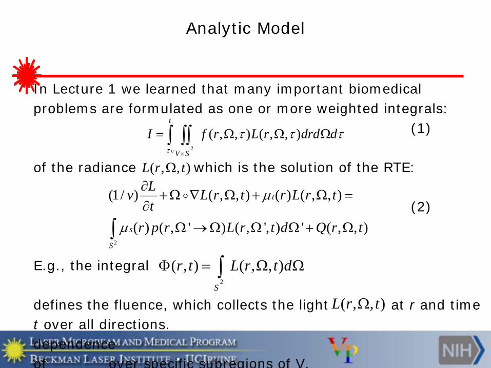
In Lecture 1 we learned that many important biomedical problems are formulated as one or more weighted integrals: (1) of the radiance which is the solution of the RTE: (2) E.g., the integral defines the fluence, which collects the light at r and time t over all directions. dependence of over specific subregions of V.

( , , )L r tΩ

2

(1/ ) ( , , ) ( ) ( , , )

( ) ( , ' ) ( , ', ) ' ( , , )

t

s

S

Lv L r t r L r tt

r p r L r t d Q r t

µ

µ

∂+Ω ∇ Ω + Ω =

∂Ω →Ω Ω Ω + Ω∫

2

( , ) ( , , )S

r t L r t dΦ = Ω Ω∫

0 2

( , , ) ( , , )t

V S

I f r L r drd dτ

τ τ τ×

= Ω Ω Ω∫ ∫∫

( , , )L r tΩ

L A M M P

Analytic Model Steady State

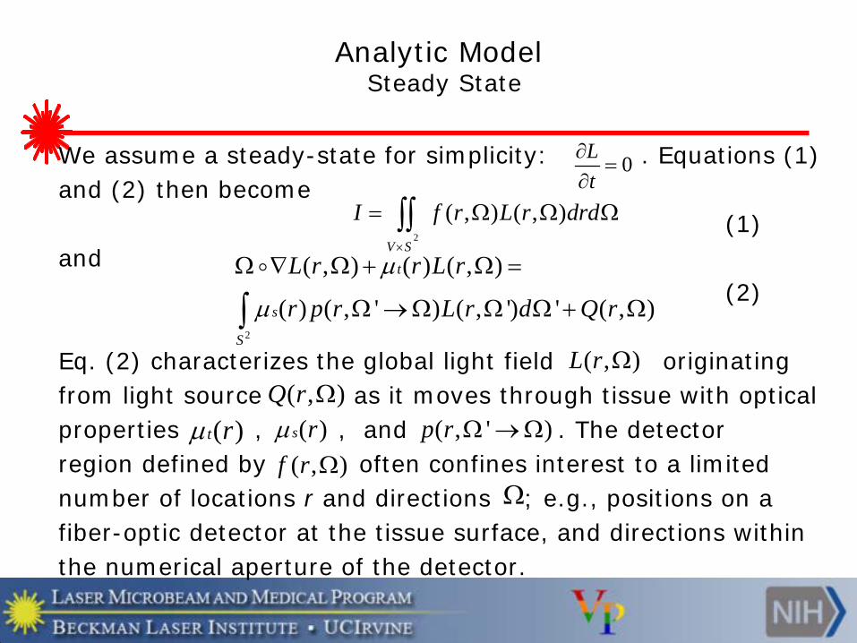
We assume a steady-state for simplicity: . Equations (1) and (2) then become (1) and (2) Eq. (2) characterizes the global light field originating from light source as it moves through tissue with optical properties , , and . The detector region defined by often confines interest to a limited number of locations r and directions ; e.g., positions on a fiber-optic detector at the tissue surface, and directions within the numerical aperture of the detector.

2

( , ) ( ) ( , )

( ) ( , ' ) ( , ') ' ( , )

t

s

S

L r r L r

r p r L r d Q r

µ

µ

Ω ∇ Ω + Ω =

Ω →Ω Ω Ω + Ω∫

2

( , ) ( , )V S

I f r L r drd×

= Ω Ω Ω∫∫

( , )Q r Ω( )s rµ ( , ' )p r Ω →Ω( )t rµ

0Lt

∂=

∂

( , )L r Ω

Ω( , )f r Ω

L A M M P

Analytic Model: Methods of Solution

Equations (1) and (2) constitute the analytic model for the RTE: (1) and (2) When the optical properties and the source are identified, any one of many deterministic numerical methods (finite difference, finite element, quadrature, etc.) can be used to produce an approximation to and, with specification of , to I as well. Sharp error bounds are hard to determine, however. Our focus is on Monte Carlo methods whose error analysis is easy, though statistical in nature.

2

( , ) ( ) ( , )

( ) ( , ' ) ( , ') ' ( , )

t

s

S

L r r L r

r p r L r d Q r

µ

µ

Ω ∇ Ω + Ω =

Ω →Ω Ω Ω + Ω∫

2

( , ) ( , )V S

I f r L r drd×

= Ω Ω Ω∫∫

( , )L r Ω ( , )f r Ω

L A M M P

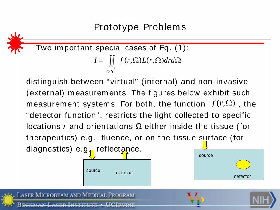
Prototype Problems

Two important special cases of Eq. (1):

distinguish between “virtual” (internal) and non-invasive (external) measurements The figures below exhibit such measurement systems. For both, the function , the “detector function”, restricts the light collected to specific locations r and orientations Ω either inside the tissue (for therapeutics) e.g., fluence, or on the tissue surface (for diagnostics) e.g., reflectance.

source

source

detector

2

( , ) ( , )V S

I f r L r drd×

= Ω Ω Ω∫∫

( , )f r Ω

detector

L A M M P

Example: Spatially-Resolved Diffuse Reflectance

where (ρ2 = x2 + y2) and S2- designates the full hemisphere of exiting directions at the tissue surface, z = 0 (matched n’s) The variables/parameters of interest to vary: Distance between source(s) & detector(s), Number and locations of detectors. In practice, light is collected over reduced numerical apertures and small surface areas that include the desired values of ρ; that is,

ρ

2

( ) ( , ) ( , , 0, )ρ−∆

= Ω = Ω Ω∫∫ ∫r S

R f r L x y z d dr

,( ) ( , , 0, )ρ

ρ ρρ

∆ ∆

∆Ω×∆

ΩΩ ≈ = Ω Ω

∆Ω×∆∫∫n

R L x y z d d

L A M M P

Example: Time-Resolved Diffuse Reflectance

Time-resolved measurements depend on introduction of a pulsed light source and collection of light that arrives at each detector at different times (equivalently, distances traversed) For both spatially- and time-resolved measurements, avoiding redundancy requires intelligent placement of detectors. This means positioning them for maximal sensitivity to different optical measures; e.g., absorption and scattering rates.

( , , ) ( , , 0, , )ρ ∆ ∆

∆Ω×∆

ΩΩ ≈ = Ω Ω

∆Ω×∆∫∫

t

nR t L x y z t d dt

t

L A M M P

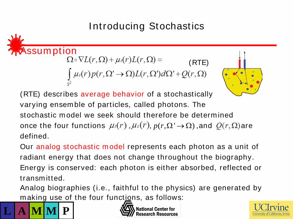
Introducing Stochastics

Assumption (RTE) (RTE) describes average behavior of a stochastically varying ensemble of particles, called photons. The stochastic model we seek should therefore be determined once the four functions , , ,and are defined. Our analog stochastic model represents each photon as a unit of radiant energy that does not change throughout the biography. Energy is conserved: each photon is either absorbed, reflected or transmitted. Analog biographies (i.e., faithful to the physics) are generated by making use of the four functions, as follows:

( , ' )p r Ω →Ω

L A M M P

• Source location & direction ~

• Distances between successive collisions from r’ along ~ ; reduces to in homogeneous case (produces correct total mean free path,1/µt)

• Absorption occurs at r with probability / • Scattering at r occurs with probability / • Scattering changes in direction at r ~ The process we’ve just described is the Analog Random

Walk (ARW) process. It creates photon biographies b, each of

Introducing Stochastics

( )( ')

0( ') exp ( ' )

r r lt tr r s dsµ µ

Ω − =− + Ω∫

exp( )t tlµ µ−

( , ) / ( , )Q r Q r drdΩ Ω Ω∫

0( , ') ( , cos )p r p r µ θ=Ω Ω =

0, 0( )r Ω

L A M M P

which is characterized by the sequence of interactions it generates: b = , , . ,… , where k =# collisions (is finite with prob 1 if > 0 for a set of of positive measure), b B = sample space of photon biographies The ARW process also induces a probability measure MAN on B This analog random walk process is simple, but it is often not

an efficient way to solve complex problems. A more general stochastic, or probabilistic, model for solving RTE problems has three components: 1. Sample space B 2. Probability measure M on B 3. Random variable, or estimator, : B R. We’ll discuss some non-analog processes shortly.

Analog Random Walks

,( )k kr Ω1, 1( )r Ω 2, 2( )r Ω

ξ →

rε

L A M M P

Statistical Error Analysis

The Monte Carlo error is assessed by computing the sample mean of the variance and standard deviation The relative error is and

( )1

1 N

iN iN bξ ξ

== ∑ξ

2

1

1 ( )1

N

N i Ni

bVarN

ξ ξ=

= − − ∑2

1

1 ( )1

N

N N i Ni

bVARN

σ ξ ξ=

= = − − ∑

L A M M P

Analog Monte Carlo: Photon Biographies in Cervical Tissue

L A M M P

Making the Movie: Input

Input: Tissue geometry & composition (dimensions, material decomposition, optical properties) Light source , initial collisions Intercollision transport T(r’→ 𝑟𝑟,Ω)= Collision mechanics ( 𝑟𝑟,Ω′ → Ω))= µs(r) /µt(r) 𝑝𝑝(𝑟𝑟,Ω′ → Ω) Termination (tally mechanism, escape, detector function f) Notice: Q, T, C characterize the integro-differential RTE, the steady state version of which is: (RTE)

'

0

( ') exp( ( ' ) )r r

t tr r s dsµ µ−

− + Ω∫

( , )Q r Ω

C

( , ) ( ' , ) ( ', ) 'S r T r r Q r drΩ = → Ω Ω∫

L A M M P

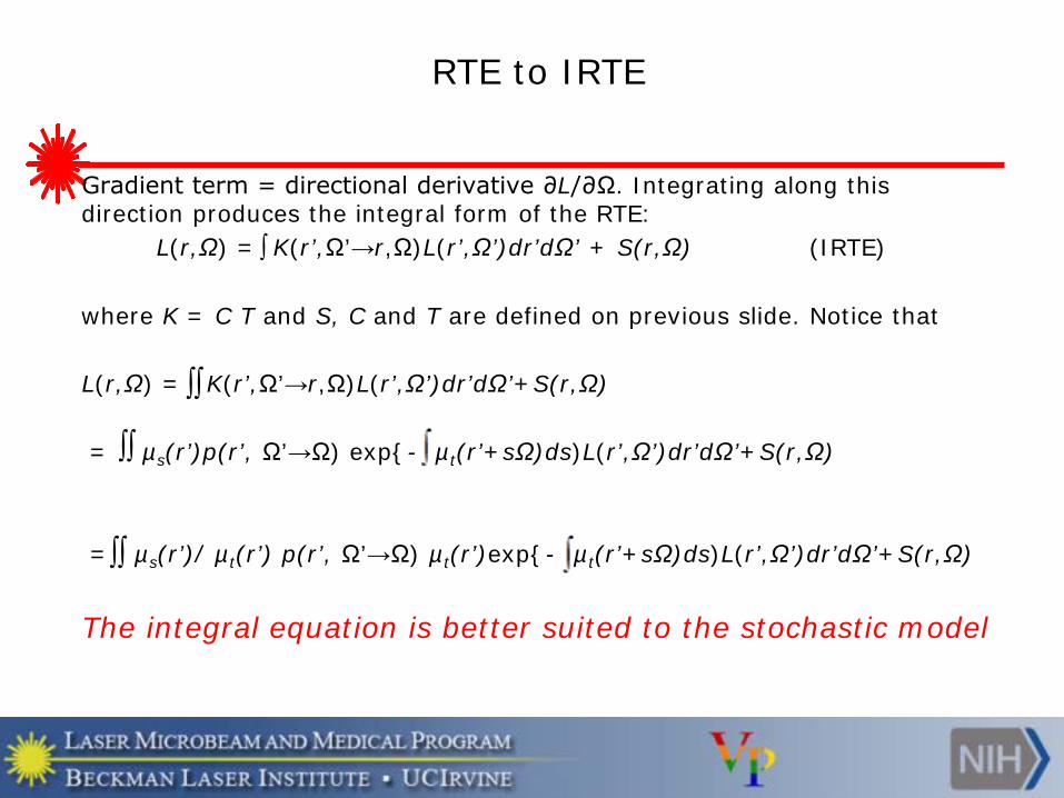
Gradient term = directional derivative ∂L/∂Ω. Integrating along this direction produces the integral form of the RTE: L(r,Ω) = K(r’,Ω’→r,Ω)L(r’,Ω’)dr’dΩ’ + S(r,Ω) (IRTE) where K = C·T and S, C and T are defined on previous slide. Notice that L(r,Ω) = K(r’,Ω’→r,Ω)L(r’,Ω’)dr’dΩ’+S(r,Ω) = µs(r’)p(r’, Ω’→Ω) exp- µt(r’+sΩ)ds)L(r’,Ω’)dr’dΩ’+S(r,Ω) = µs(r’)/ µt(r’) p(r’, Ω’→Ω) µt(r’)exp- µt(r’+sΩ)ds)L(r’,Ω’)dr’dΩ’+S(r,Ω)

The integral equation is better suited to the stochastic model

RTE to IRTE

∫

∫∫

∫∫

∫∫

L A M M P

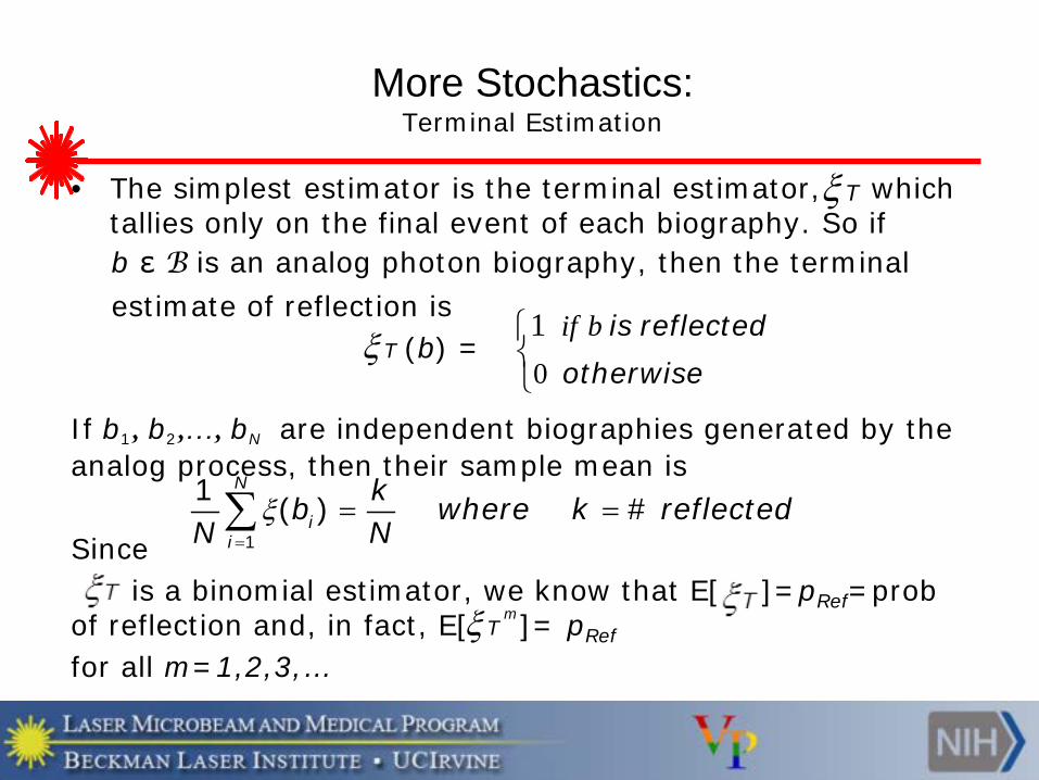
• The simplest estimator is the terminal estimator, which tallies only on the final event of each biography. So if

b ε B is an analog photon biography, then the terminal estimate of reflection is (b) = If b1, b2,…, bN are independent biographies generated by the analog process, then their sample mean is Since is a binomial estimator, we know that E[ ]=pRef=prob of reflection and, in fact, E[ ]= pRef for all m=1,2,3,…

More Stochastics: Terminal Estimation

1

1 ( ) #N

ii

kb where k reflectedN N

ξ=

= =∑

01 if b

is reflectedotherwise

Tξ

mTξ

Tξ

L A M M P

More Stochastics: Terminal Estimation (cont’d)

It follows that Var [ ] = p(1-p) RE [ ] = So if one places a detector very far from the source, the signal will be essentially 0 there, and terminal estimation will be useless. Remedy: Imagine that each photon is a packet with weight W of many individual photons that are transported together by ARW process. Set W = 1 initially. (W is just a scaling factor)

2(1 ) (1 ) 0p p p as pp p− −

= → ∞ →

L A M M P

Discrete Absorption Weighting (DAW)

In the ARW process, each photon is assigned a weight of 1 which never changes. Instead, think of each photon as a packet of photons with initial “strength” W = 1(scaling factor) that diminishes at each collision by absorbing a partial weight at that collision. The remaining weight, scatters there and continues in a new direction. This describes another random walk process, discrete absorption weighting, DAW, and a new estimator Characteristics of DAW: 1. Every photon packet exits the tissue 2. DAW takes more run time 3.

µµ

a

tW

Var Var[ ] [ ]DAW Tξ ξ<

DAWξ

L A M M P

Sketch of proof of (3) Possible values of are It is intuitively clear (and rigorously provable) that Where = probability that biography makes exactly collisions before exit. However, since each

Discrete Absorption Weighting (DAW) (cont’d)

L A M M P

DAW Movie

L A M M P

Analog vs. DAW Comparison Varying Source-Detector Separation

L A M M P

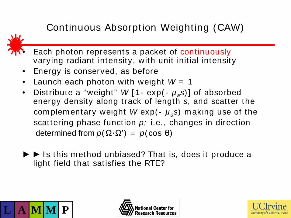
Continuous Absorption Weighting (CAW)

• Each photon represents a packet of continuously varying radiant intensity, with unit initial intensity

• Energy is conserved, as before • Launch each photon with weight W = 1 • Distribute a “weight” W·[1- exp(- µas)] of absorbed

energy density along track of length s, and scatter the complementary weight W·exp(- µas) making use of the scattering phase function p; i.e., changes in direction determined from p(Ω·Ω’) = p(cos θ) Is this method unbiased? That is, does it produce a

light field that satisfies the RTE?

L A M M P

Continuous Absorption Weighting (CAW)

• Each photon represents a packet of continuously varying radiant intensity, with unit initial intensity

• Energy is conserved, as before • Launch each photon with weight W = 1 • Distribute a “weight” W·[1- exp(- µas)] of absorbed

energy density along track of length s, and scatter the complementary weight W·exp(- µas) making use of the scattering phase function p; i.e., changes in direction determined from p(Ω·Ω’) = p(cos θ) Is this method unbiased? That is, does it produce a

light field that satisfies the RTE? Not unless the intercollision distances d ~ Rather than exp( )t tdµ µ−

L A M M P

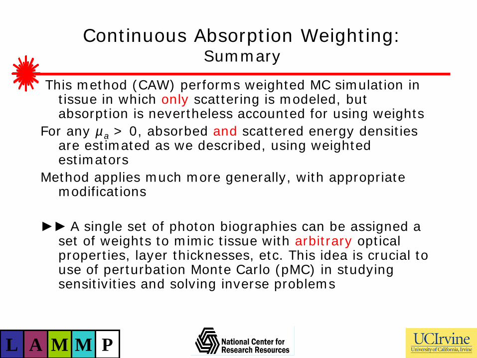
Continuous Absorption Weighting: Summary

This method (CAW) performs weighted MC simulation in tissue in which only scattering is modeled, but absorption is nevertheless accounted for using weights

For any µa > 0, absorbed and scattered energy densities are estimated as we described, using weighted estimators

Method applies much more generally, with appropriate modifications

A single set of photon biographies can be assigned a

set of weights to mimic tissue with arbitrary optical properties, layer thicknesses, etc. This idea is crucial to use of perturbation Monte Carlo (pMC) in studying sensitivities and solving inverse problems

L A M M P

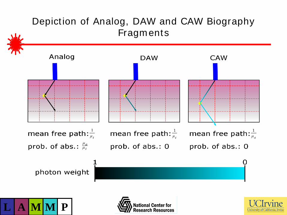
Depiction of Analog, DAW and CAW Biography Fragments

L A M M P

Analog 100k histories (+5)

L A M M P

DAW 100k histories (+5)

L A M M P

CAW 100k histories (+5)

L A M M P

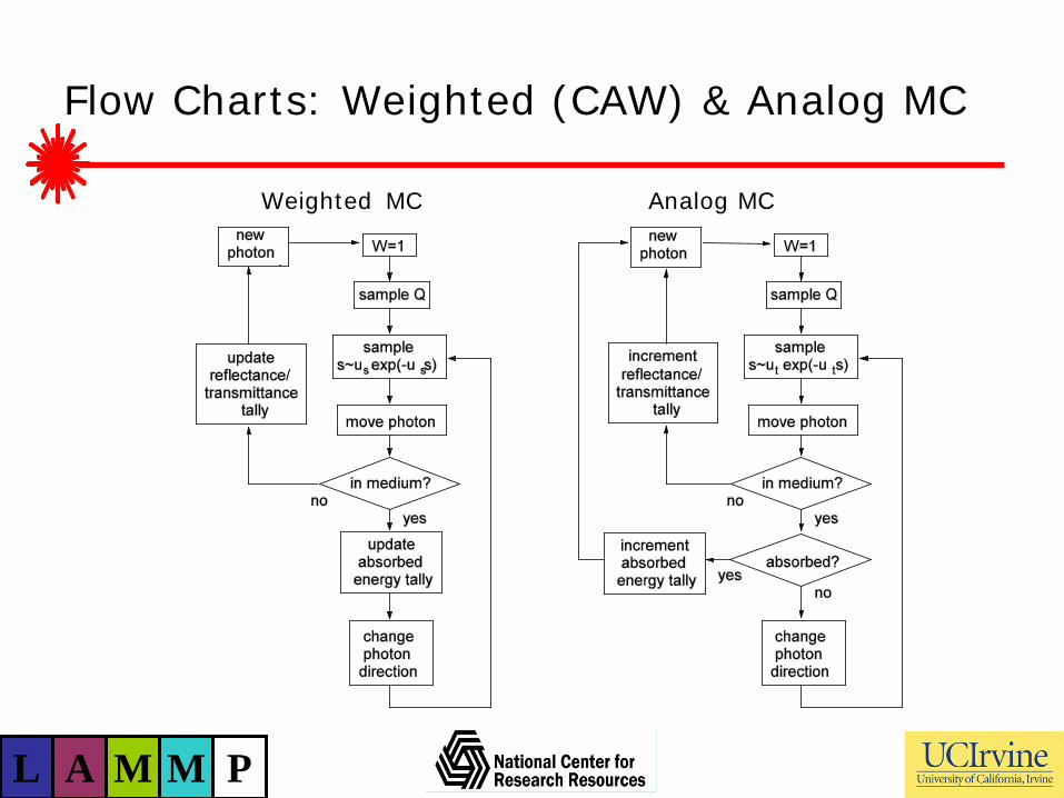
Flow Charts: Weighted (CAW) & Analog MC

Weighted MC Analog MC

L A M M P

MC Model Connections

Analytic Model:

Г, RTE + BC + f Stochastic Model:

Ω, M, ξ

Probability Model: Normalized Q, T, C

Simulation Model: Q, T, C, …,T, (P0,…,Pk) , ξ(P0,…, Pk)

⌠ fL= ⌠ ξdM

←

Sample Densities Generate Output

Generate

Input →

↓ ↑

L A M M P

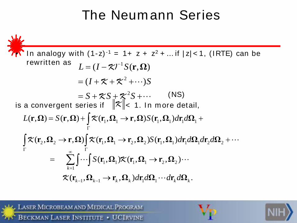
The Neumann Series

• In analogy with (1-z)-1 = 1+ z + z2 +… if |z|<1, (IRTE) can be rewritten as

(NS) is a convergent series if < 1. In more detail,

1

2

2

( ( , )( )

L I SI S

S S S

−= −

= + + + ⋅⋅⋅

= + + + ⋅⋅⋅

r ΩK)

K K

K KK

1 1 1 1 1 1

2 2 1 1 2 2 1 1 1 1 2 2

( , ) ( , ) ( , , ) ( , )

( , , ) ( , , ) ( , )

L S S d d

S d d d dΓ

Γ Γ

= + → +

→ → +

∫

∫ ∫

r Ω r Ω r Ω r Ω r Ω r Ω

r Ω r Ω r Ω r Ω r Ω r Ω r Ω

K

K K

1 1 1 1 2 21

1 1 1 1

( , ) ( , , )

( , , ) .k

k k k k k k

S

d d d d

∞

=

− −

= →

→

∑∫ ∫ r Ω r Ω r Ω

r Ω r Ω r Ω r Ω

K

K

L A M M P

The Neumann Series

• To show that

• we expand L in its Neumann series, multiply by f and integrate:

and then recognize the result as the representation

1 1 1 1 1 1

2 2 1 1 2 2 1 1 1 1 2 2

( , ) ( , ) ( , ) ( , )

( , ) ( , , ) ( , )

( , ) ( , , ) ( , , ) ( , )

Γ Γ

Γ Γ

Γ Γ Γ

Ω Ω = Ω Ω+

Ω Ω → +

Ω Ω → → +

∫ ∫

∫ ∫

∫ ∫ ∫

f r L drd f r S drd

f r drd S d d

f r drd S d d d d

r Ω r Ω

r Ω r Ω r Ω r Ω

r Ω r Ω r Ω r Ω r Ω r Ω r Ω

K

K K

( )ξ= ∫I b dB

M

( , ) ( , ) ( )I f r L r drd b dξΓ

= Ω Ω Ω =∫ ∫B

M

L A M M P

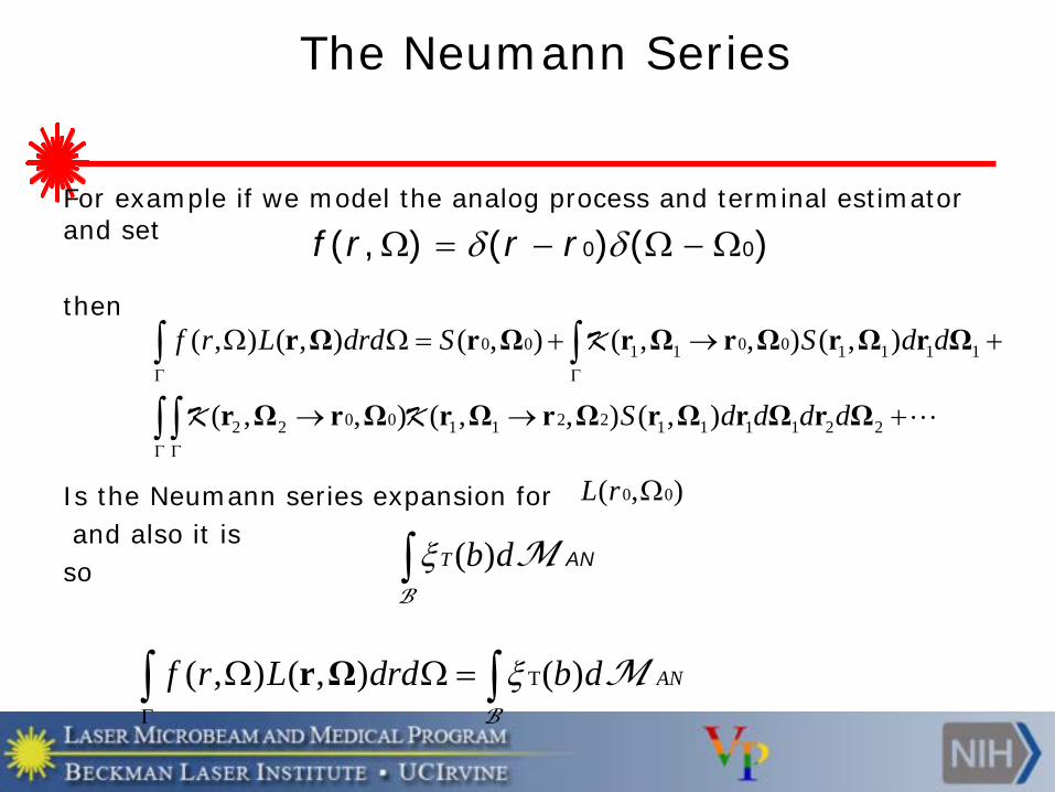
The Neumann Series

For example if we model the analog process and terminal estimator and set

then

Is the Neumann series expansion for and also it is so ( ) ANξ∫ T b d

B

M

0 0( , ) ( ) ( )f r r rδ δΩ = − Ω − Ω

T( , ) ( , ) ( )ξΓ

Ω Ω =∫ ∫ ANf r L drd b dr ΩB

M

0 0 0 01 1 1 1 1 1

0 0 2 22 2 1 1 1 1 1 1 2 2

( , ) ( , ) ( , ) ( , , ) ( , )

( , , ) ( , , ) ( , )Γ Γ

Γ Γ

Ω Ω = + → +

→ → +

∫ ∫

∫ ∫

f r L drd S S d d

S d d d d

r Ω r Ω r Ω r Ω r Ω r Ω

r Ω r Ω r Ω r Ω r Ω r Ω r Ω

K

K K

0 0( , )ΩL r

L A M M P

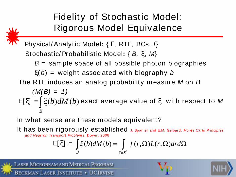
Fidelity of Stochastic Model: Rigorous Model Equivalence

Physical/Analytic Model: Γ, RTE, BCs, f Stochastic/Probabilistic Model: B, ξ, M B = sample space of all possible photon biographies ξ(b) = weight associated with biography b The RTE induces an analog probability measure M on B (M(B) = 1) E[ξ] = exact average value of ξ with respect to M In what sense are these models equivalent? It has been rigorously established J. Spanier and E.M. Gelbard, Monte Carlo Principles

and Neutron Transport Problems, Dover, 2008

E[ξ] = 2

( ) ( ) ( , ) ( , )B S

b dM b f r L r drdξΓ×

= Ω Ω Ω∫ ∫

ξ( ) ( )B

b dM b∫

L A M M P

Take Home Messages

• Analog Monte Carlo is easy and intuitive • Weighted Monte Carlo is preferred in most cases • Intuition is not a reliable indicator in simulation • The Neumann series is key to proving

unbiasedness and equivalence of analytic and stochastic models

There is room for more mathematicians to work in this area

L A M M P

Thanks to

Carole Hayakawa, Jennifer Nguyen and Shuang Zhao for creating the movies and some of the figures I used.