REVIEW OF IMAGE ENHANCEMENT TECHNIQUES USING HISTOGRAM EQUALIZATION
1
Digital Image Processing
Lecture # 4Histogram Equalization & Matching

2
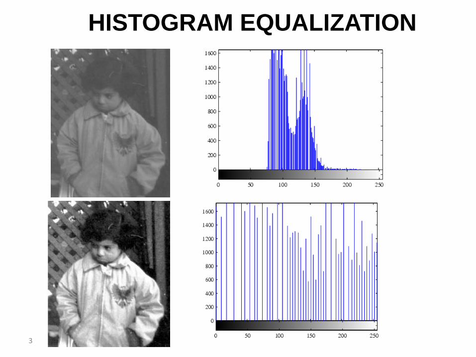
Histogram Equalization
Histogram equalization re-assigns the intensity values of pixels in the input
image such that the output image contains a uniform distribution of intensities
3
HISTOGRAM EQUALIZATION

4
AERIAL PHOTOGRAPH OF THE PENTAGON
Resulting image uses more of dynamic range.
Resulting histogram almost, but not completely, flat.

5
The Probability Distribution Function of an Image
255
0
Let I
g
A h g
Note that since is the number of pixels in
with value ,
is the number of pixels in . That is if is
rows by columns then .
Ih g
I g
A I I
R C A R C
Then,
1
I Ip g h gA
This is the probability that an arbitrary pixel from I has value g.

6
The Probability Distribution Function of an Image
• p(g) is the fraction of pixels in an image that have
intensity value g.
• p(g) is the probability that a pixel randomly selected
from the given image has intensity value g.
• Whereas the sum of the histogram h(g) over all g from
0 to 255 is equal to the number of pixels in the image,
the sum of p(g) over all g is 1.
• p is the normalized histogram of the image

7
The Cumulative Distribution Function of an Image
0
2550 0
0
1
,
g
Ig g
I I I
I
h
P g p hA
h
This is the probability that any given pixel from I has value less than or equal to g.
Let q = I(r,c) be the value of a randomly
selected pixel from I. Let g be a specific gray
level. The probability that q ≤ g is given by
where hI(γ ) is
the histogram of
image I.

8
The Cumulative Distribution Function of an Image
0
2550 0
0
1
,
g
Ig g
I I I
I
h
P g p hA
h
This is the probability that any given pixel from I has value less than or equal to g.
Let q = I(r,c) be the value of a randomly
selected pixel from I. Let g be a specific gray
level. The probability that q ≤ g is given by
where hI(γ ) is
the histogram of
image I.
Also called CDF for “Cumulative Distribution Function”.

9
The Cumulative Distribution Function of an Image
• P(g) is the fraction of pixels in an image that have intensity
values less than or equal to g.
• P(g) is the probability that a pixel randomly selected from
the given band has an intensity value less than or equal to
g.
• P(g) is the cumulative (or running) sum of p(g) from 0
through g inclusive.
• P(0) = p(0) and P(255) = 1;

10
Histogram Equalization
Let IP
The CDF itself is used as the LUT.
be the cumulative (probability) distribution function of I.
Task: remap image I so that its histogram is as close to
constant as possible

11
Histogram Equalization
The CDF (cumulative distribution) is the LUT for remapping.
CDF

12
Histogram Equalization
The CDF (cumulative distribution) is the LUT for remapping.
LUT

13
Histogram Equalization
The CDF (cumulative distribution) is the LUT for remapping.
LUT

14
Histogram Equalization

15
Histogram Equalization
after
before
Luminosity
, 255 , .IJ r c P I r c

16
HISTOGRAM EQUALIZATION IMPLEMENTATION
0 0 0 0
1 1 1 1
4 5 6 6
8 8 8 8
0
4
6
9
2 2 2 2
4 4 4 4
5 5 7 7
9 9 9 9
2
5
7
9
0 1 2 3 4 5 6 7 8 9Gray levels
Counts (h(rk)) 5 4 0 0 2 1 3 0 4 1r0 r1 r2 r3 r4 r5 r6
5/20 4/200 0
2/20 1/20 3/20 0 4/20 1/20Normalized h (P(rk))
cdf F(rk) 5/20 9/20 11/20 12/20 15/20 19/20 20/20
sk =round(9•F(rk)) 2 4 5 5 7 9 9
s0 s1 s2 s3 s4 s5 s6
17
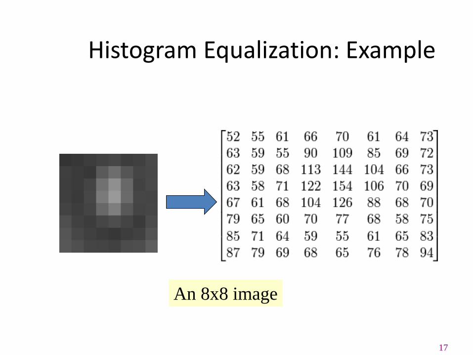
Histogram Equalization: Example
An 8x8 image

18
Histogram Equalization: Example
Image Histogram (Non-zero values)
Fill in the following table/histogram

19
Histogram Equalization: Example
Image Histogram (Non-zero values shown)

20
Histogram Equalization: Example

21
Histogram Equalization: Example
Cumulative Distribution Function (cdf)
Image Histogram/Prob Mass Function

22
Histogram Equalization: Example
Cumulative Distribution Function (cdf)

23
Histogram Equalization: Example
Cumulative Distribution Function (cdf)

24
Histogram Equalization: Example
Normalized Cumulative Distribution Function (cdf)
Divide each value by total number of
pixels (64) to get the normalized cdf

25
Histogram Equalization: Example
, 255 , .IJ r c P I r c
Original Image
183
( )(255. )
(255. 46 / 64 )
183
cdf rs round
M N
s round
s
(255. ( ))s round cdf r
If cdf is normalized
If cdf is NOT normalized

26
Histogram Equalization: Example

27
Histogram Equalization: Example
Original Image Corresponding histogram (red) and cumulative
histogram (black)
Image after histogram equalization Corresponding histogram (red) and cumulative
histogram (black)

28
Histogram Equalization: ExampleD
ark
im
ag
eB
rig
ht
imag
e
Equalized Histogram
Equalized Histogram

29
Histogram Equalization: ExampleL
ow
co
ntr
ast
Hig
h C
on
trast
Equalized Histogram
Equalized Histogram

30
HISTOGRAM MATCHING (SPECIFICATION)
• HISTOGRAM EQUALIZATION DOES NOT ALLOWINTERACTIVE IMAGE ENHANCEMENT ANDGENERATES ONLY ONE RESULT: ANAPPROXIMATION TO A UNIFORM HISTOGRAM.
• SOMETIMES THOUGH, WE NEED TO BE ABLE TOSPECIFY PARTICULAR HISTOGRAM SHAPESCAPABLE OF HIGHLIGHTING CERTAIN GRAY-LEVELRANGES.

31
HISTOGRAM SPECIFICATION• THE PROCEDURE FOR HISTOGRAM-SPECIFICATION BASED
ENHANCEMENT IS:
– EQUALIZE THE LEVELS OF THE ORIGINAL IMAGE USING:
k
j
j
kn
nrTs
0
)(
n: total number of pixels,
nj: number of pixels with gray level rj,
L: number of discrete gray levels
32
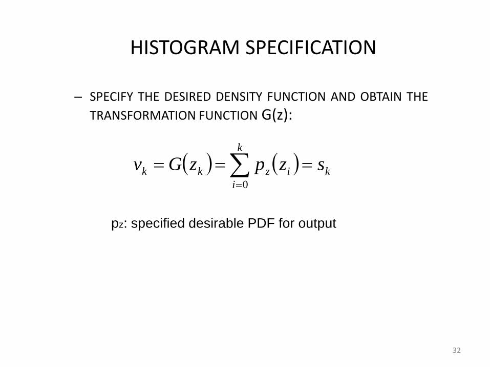
HISTOGRAM SPECIFICATION
– SPECIFY THE DESIRED DENSITY FUNCTION AND OBTAIN THE
TRANSFORMATION FUNCTION G(z):
pz: specified desirable PDF for output
ki
k
i
zkk szpzGv 0

33
HISTOGRAM SPECIFICATION
• THE NEW, PROCESSED VERSION OF THEORIGINAL IMAGE CONSISTS OF GRAYLEVELS CHARACTERIZED BY THE SPECIFIEDDENSITY pz(z).
)]([ )( 11 rTGzsGz In essence:
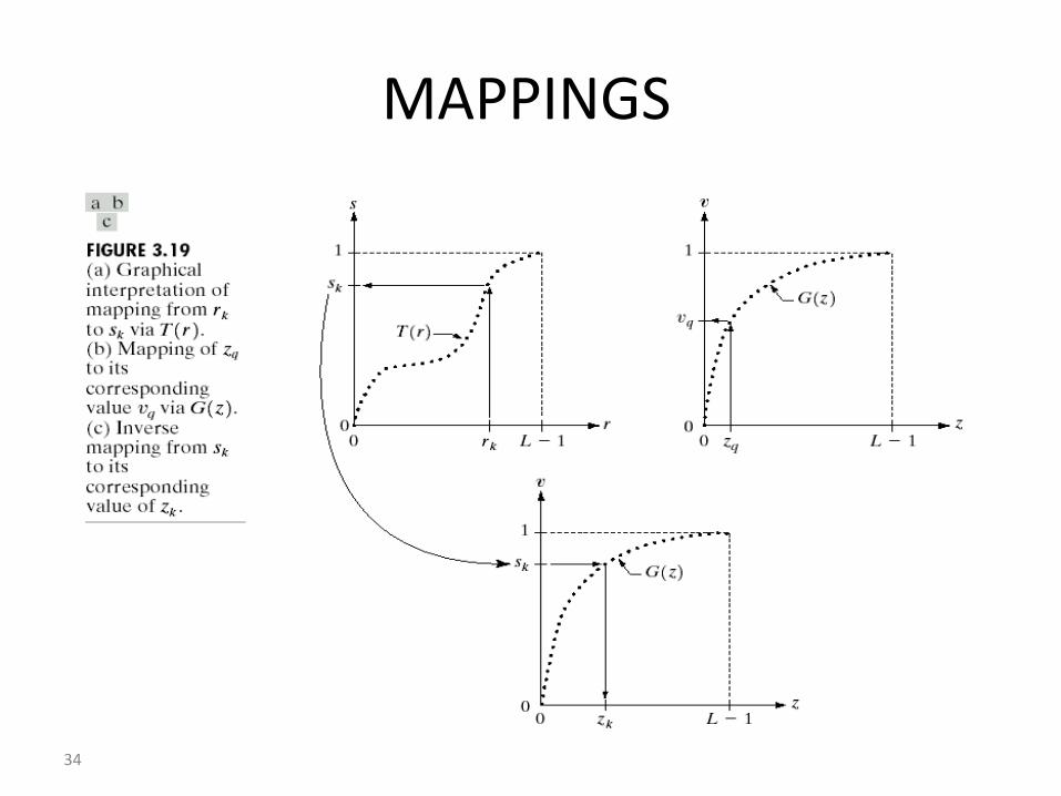
34
MAPPINGS
35
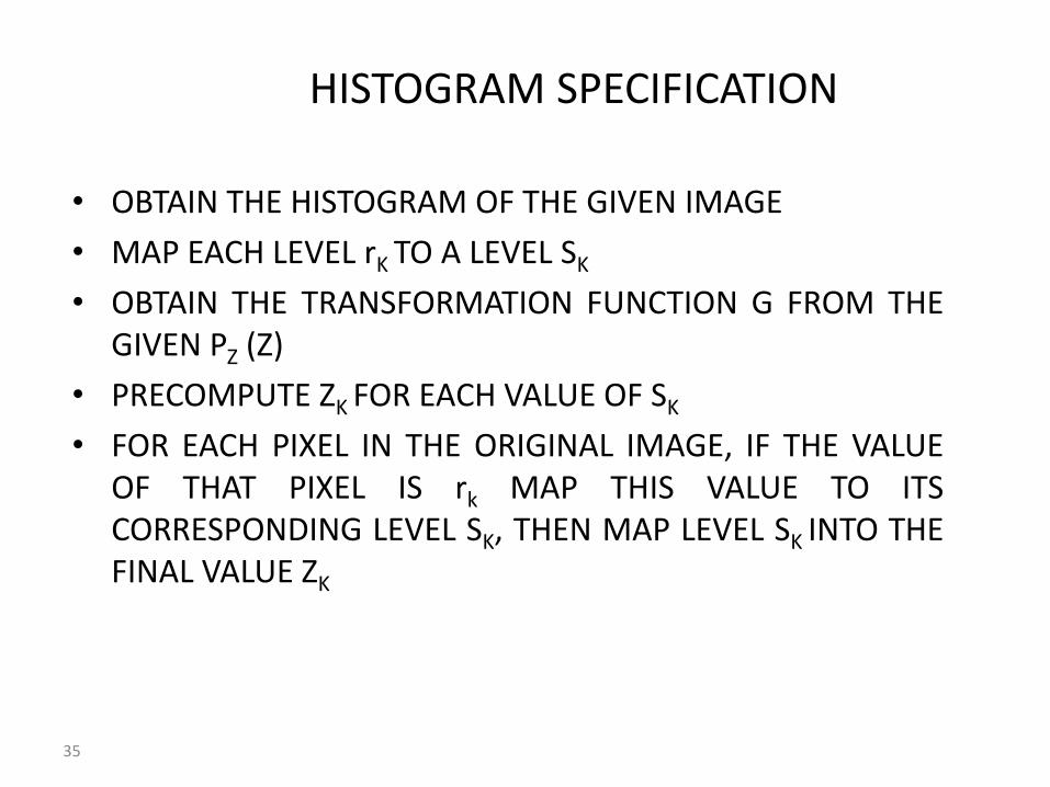
HISTOGRAM SPECIFICATION
• OBTAIN THE HISTOGRAM OF THE GIVEN IMAGE
• MAP EACH LEVEL rK TO A LEVEL SK
• OBTAIN THE TRANSFORMATION FUNCTION G FROM THEGIVEN PZ (Z)
• PRECOMPUTE ZK FOR EACH VALUE OF SK
• FOR EACH PIXEL IN THE ORIGINAL IMAGE, IF THE VALUEOF THAT PIXEL IS rk MAP THIS VALUE TO ITSCORRESPONDING LEVEL SK, THEN MAP LEVEL SK INTO THEFINAL VALUE ZK
36
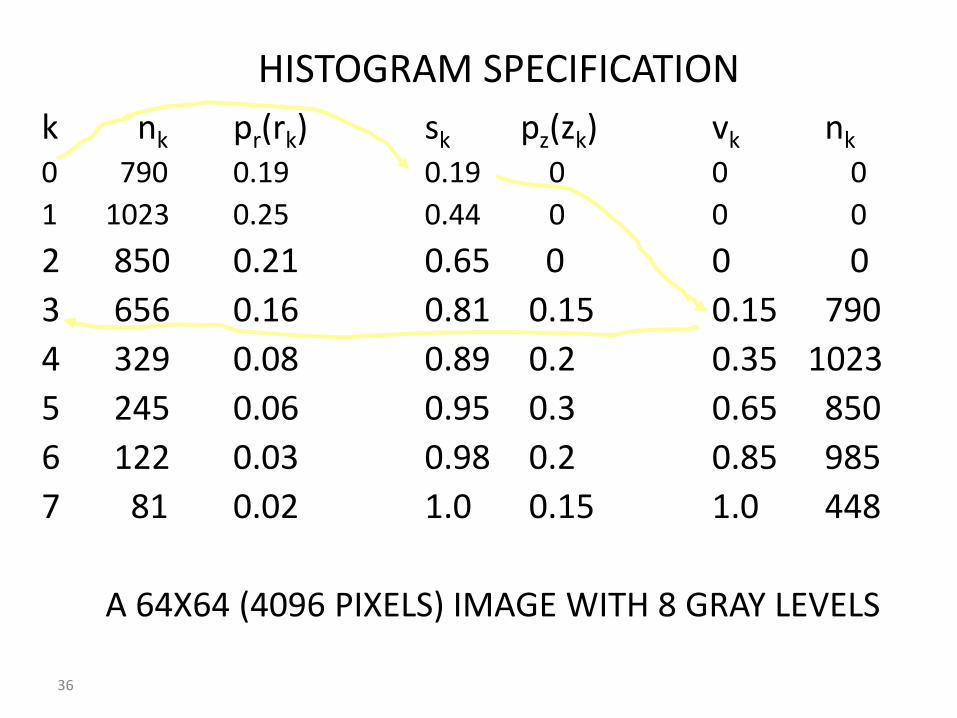
HISTOGRAM SPECIFICATION
k nk pr(rk) sk pz(zk) vk nk
0 790 0.19 0.19 0 0 0
1 1023 0.25 0.44 0 0 0
2 850 0.21 0.65 0 0 0
3 656 0.16 0.81 0.15 0.15 790
4 329 0.08 0.89 0.2 0.35 1023
5 245 0.06 0.95 0.3 0.65 850
6 122 0.03 0.98 0.2 0.85 985
7 81 0.02 1.0 0.15 1.0 448
A 64X64 (4096 PIXELS) IMAGE WITH 8 GRAY LEVELS

37
IMAGE ENHANCEMENT IN THE
SPATIAL DOMAIN

38
IMAGE ENHANCEMENT IN THE
SPATIAL DOMAIN

39

40
GLOBAL/LOCAL HISTOGRAM EQUALIZATION
• IT MAY BE NECESSARY TO ENHANCE DETAILS OVER SMALL AREAS IN THEIMAGE
• THE NUMBER OF PIXELS IN THESE AREAS MAY HAVE NEGLIGIBLE INFLUENCEON THE COMPUTATION OF A GLOBAL TRANSFORMATION WHOSE SHAPEDOES NOT NECESSARILY GUARANTEE THE DESIRED LOCAL ENHANCEMENT
• DEVISE TRANSFORMATION FUNCTIONS BASED ON THE GRAY LEVELDISTRIBUTION IN THE NEIGHBORHOOD OF EVERY PIXEL IN THE IMAGE
• THE PROCEDURE IS:– DEFINE A SQUARE (OR RECTANGULAR) NEIGHBORHOOD AND MOVE THE
CENTER OF THIS AREA FROM PIXEL TO PIXEL.– AT EACH LOCATION, THE HISTOGRAM OF THE POINTS IN THE
NEIGHBORHOOD IS COMPUTED AND EITHER A HISTOGRAMEQUALIZATION OR HISTOGRAM SPECIFICATION TRANSFORMATIONFUNCTION IS OBTAINED.
– THIS FUNCTION IS FINALLY USED TO MAP THE GRAY LEVEL OF THE PIXELCENTERED IN THE NEIGHBORHOOD.
– THE CENTER IS THEN MOVED TO AN ADJACENT PIXEL LOCATION AND THEPROCEDURE IS REPEATED.

41
GLOBAL/LOCAL HISTOGRAM EQUALIZATION

42
USE OF HISTOGRAM STATISTICS FOR IMAGE ENHANCEMENT (Global)
• LET r REPRESENT A GRAY LEVEL IN THE IMAGE [0, L-1], AND LET p(ri )DENOTE THE NORMALIZED HISTOGRAM COMPONENTCORRESPONDING TO THE ith VALUE OF r.
• THE nth MOMENT OF r ABOUT ITS MEAN IS DEFINED AS
• WHERE m IS THE MEAN VALUE OF r (AVERAGE GRAY LEVEL)
i
nL
i
in rpmrr
1
0
i
L
i i rprm
1
0

43
USE OF HISTOGRAM STATISTICS FOR IMAGE ENHANCEMENT (Global)
• THE SECOND MOMENT IS GIVEN BY
• WHICH IS THE VARIANCE OF r
• MEAN AS A MEASURE OF AVERAGE GRAY LEVEL IN THE IMAGE
• VARIANCE AS A MEASURE OF AVERAGE CONTRAST
i
L
i
i rpmrr
21
0
2

44
USE OF HISTOGRAM STATISTICS FOR IMAGE ENHANCEMENT (Local)
• LET (x,y) BE THE COORDINATES OF A PIXEL IN ANIMAGE, AND LET SX,Y DENOTE A NEIGBORHOOD OFSPECIFIED SIZE, CENTERED AT (x,y)
• THE MEAN VALUE mSXY OF THE PIXELS IN SX,Y IS
• THE GRAY LEVEL VARIANCE OF THE PIXELS INREGION SX,Y IS GIVEN BY
ts
Sts
tss rprmxy
xy ,
,
,
ts
Sts
stsS rpmrxy
xyxy ,
,
2
,
2
45
USE OF HISTOGRAM STATISTICS FOR IMAGE ENHANCEMENT
• THE GLOBAL MEAN AND VARIANCE ARE MEASUREDOVER AN ENTIRE IMAGE AND ARE USEFUL FORGROSS ADJUSTMENTS OF OVERALL INTENSITY ANDCONTRAST.
• A USE OF THESE MEASURES IN LOCALENHANCEMENT IS, WHERE THE LOCAL MEAN ANDVARIANCE ARE USED AS THE BASIS FOR MAKINGCHANGES THAT DEPEND ON IMAGECHARACTERISTICS IN A PREDEFINED REGION ABOUTEACH PIXEL IN THE IMAGE.

46
TUNGSTEN FILAMENT IMAGE

47
USE OF HISTOGRAM STATISTICS FOR IMAGE ENHANCEMENT
• A PIXEL AT POINT (x,y) IS CONSIDERED IF:– mSXY ≤ k0MG, where k0 is a positive constant less than 1.0, and MG is
global mean
– σsxy ≤ k2DG, where DG is the global standard deviation and k2 is apositive constant
– k1DG ≤ σsxy ,, with k1 < k2
• A PIXEL THAT MEETS ALL ABOVE CONDITIONS ISPROCESSED SIMPLY BY MULTIPLYING IT BY A SPECIFIEDCONSTANT, E, TO INCREASE OR DECREASE THE VALUE OFITS GRAY LEVEL RELATIVE TO THE REST OF THE IMAGE.
• THE VALUES OF PIXELS THAT DO NOT MEET THEENHANCEMENT CONDITIONS ARE LEFT UNCHANGED.

48
IMAGE ENHANCEMENT IN THESPATIAL DOMAIN

49
IMAGE ENHANCEMENT IN THE
SPATIAL DOMAIN

Readings from Book (3rd Edn.)
• 3.3 Histogram

51
Acknowledgements
Statistical Pattern Recognition: A Review – A.K Jain et al., PAMI (22) 2000
Pattern Recognition and Analysis Course – A.K. Jain, MSU
Pattern Classification” by Duda et al., John Wiley & Sons.
Digital Image Processing”, Rafael C. Gonzalez & Richard E. Woods, Addison-Wesley, 2002
Machine Vision: Automated Visual Inspection and Robot Vision”, David Vernon, Prentice Hall, 1991
www.eu.aibo.com/
Advances in Human Computer Interaction, Shane Pinder, InTech, Austria, October 2008
Mat
eria
l in
th
ese
slid
es h
as b
een
tak
en f
rom
, th
e fo
llow
ing
reso
urc
es