Lecture 3

Survival analysis

The slang

• Current life table– What is the life time now?

• Cohort life table– What is the life time of this group?

Problem• Do patients survive longer after treatment

A than after treatment B?

• Possible solutions:– ANOVA on mean survival time?– ANOVA on median survival time?

• Survival analysis– Aka. Actuarial / life table analysis

The example

Person-year of observation• In total: 15122 days ~ 41.4y• 11 patients died: 11/41.4y = 0.266 y-1

26.6 death/100y• 1000 patients in 1 y• or • 100 patients in 10y

Mortality rates• 11 of 25 patients died

• 11/25 = 44%

• When is the analysis done?

1-year survival rate• 6 patients dies the first year

• 25 patients started

• 24%

1-year survival rate• 3 patients less than 1 year

• 6/(25-3) = 27%

• Patient 7

• 24% -27%

Actuarial / life table anelysis• Patients on dialysis

• 180 day pariods

Actuarial / life table anelysis• Ni number of patients

starting a given period

Actuarial / life table anelysis• Wi number of patients

that have not yet been in the study long enough to finish this period

Actuarial / life table anelysis• Number exposed to risk:

• ni – wi/2

• Assuming that patients withdraw in the middle of the period on average.

Actuarial / life table anelysis• di : Number of patients

that died

Actuarial / life table anelysis• qi = di/(ni – wi/2)

• Proportion of patients terminating in the period

Actuarial / life table anelysis• pi = 1 - qi

• Proportion of patients surviving

Actuarial / life table anelysis• Si = pi pi-1 ...pi-N

• Cumulative proportion of surviving

• Conditional probability

Survival curves• How long will a

dialysis patient survive?

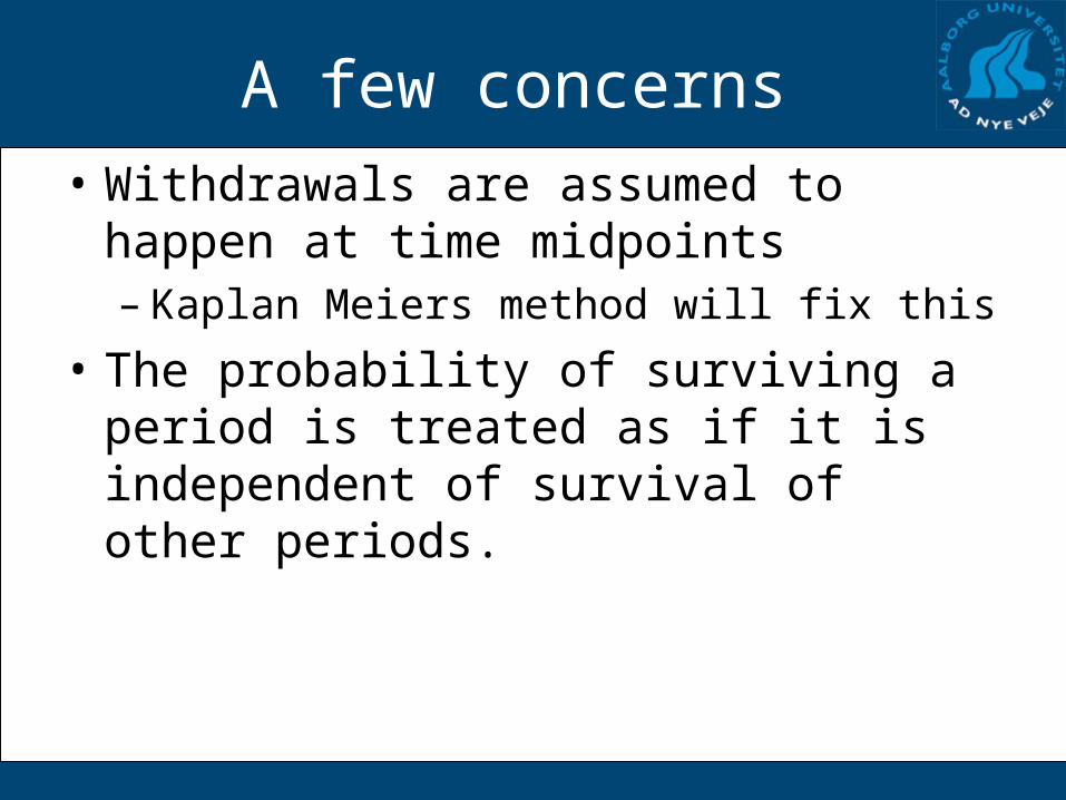
A few concerns • Withdrawals are assumed to happen at

time midpoints– Kaplan Meiers method will fix this

• The probability of surviving a period is treated as if it is independent of survival of other periods.

Kaplan-Meier product limit method

• Changes in the survival curve are calculated when an event occurs

• Withdrawals are ignored as events

Kaplan-Meier• Simple example with only

4 ”death-events”.

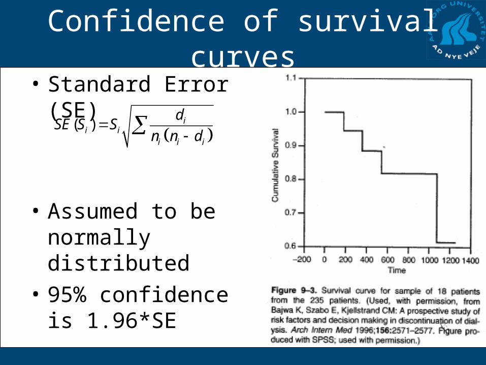
Confidence of survival curves• Standard Error (SE)

• Assumed to be normally distributed

• 95% confidence is 1.96*SE

( ) ii i

i i i

dSE S S

n n d

Confidence interval of the Kaplan-Meier method

( ) ii i

i i i

dSE S S

n n d

The Kaplan-Meier method

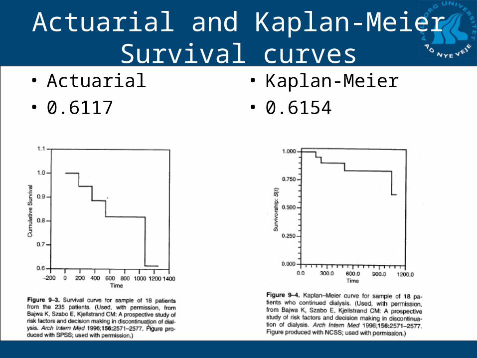
Actuarial and Kaplan-Meier Survival curves

• Actuarial• 0.6117

• Kaplan-Meier• 0.6154

Comparing survival curves

Comparing survival curves• Two principle methods

– Logrank statistics– Mantel Haenszel chi-square statistics

Logrank statistics

# #

#

deaths groupE

total

2

2 O E

E

Logrank statistics

Hazard ratio

1 1

2 2

Hazard ratio 4.13O E

O E

Mantel Haenszel chi-square statistics

Mantel Haenszel chi-square statistics

/

/

a d nOR

b c n

_ _( )

_i

Row total Col totalE a

Grand total

2

( )( )( )( )( )

( 1)i

a b b d a b c dV a

n n

2

i i

i

a E aMantel Haenszel

V a

Hazard function

dH

f c

log( )iH S