LECTURE 3: S R II

LECTURE 3:

SIMPLE REGRESSION II

Introductory EconometricsJan Zouhar

Population vs. sample regression function.

Residuals and their properties.

Goodness of fit.

Algebraic Properties of OLS Statistics

Jan Zouhar

2

Introductory Econometrics

Population Vs. Sample Regression Function

Jan ZouharIntroductory Econometrics

3

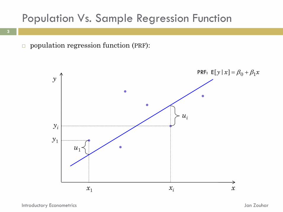
population regression function (PRF):

yi

xi x

y

x1

y1

PRF: E 0 1[ | ]y x x

ui

u1

Population Vs. Sample Regression Function (cont’d)


4

sample regression function (SRF):

yi

xi x

y

SRF: 0 1ˆ ˆy x

x1

y1

ˆiu

1u

ˆiy

1y

PRF

Goodness of Fit


5

we want to say something about how well the model fits our data

(the goal is to end up with a single number, ideally expressed as a

percentage)

we will make use of the following three things:

total sum of squares (SST)

explained sum of squares (SSE)

residual sum of squares (SSR)

2 21 1( )ˆ ˆn n

i i ii iSSR y y u

21( )n

iiSST y y

21( )ˆn

iiSSE y y

yi

xi x

yi

y

0 1ˆ ˆy x

SSTSSR

SSE

Goodness of Fit (cont’d)


6

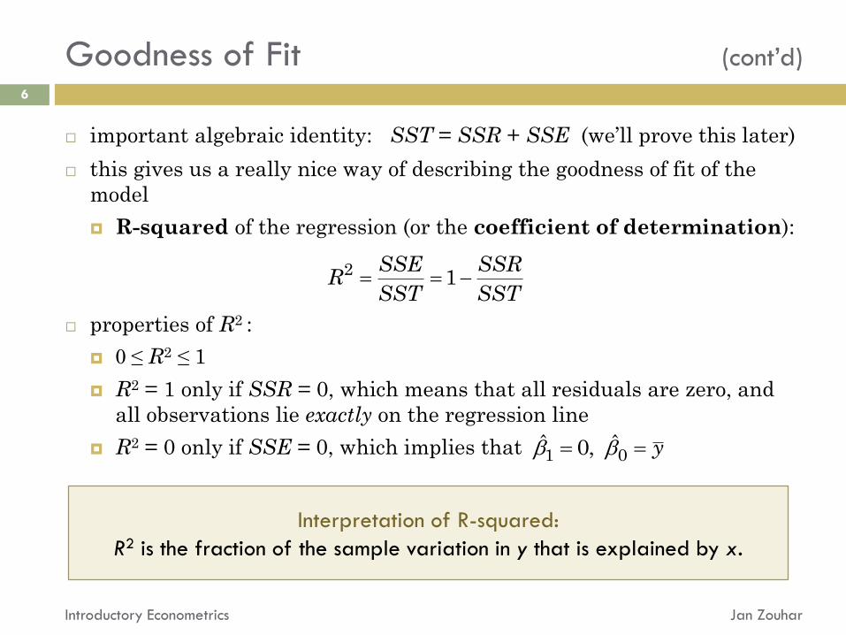
important algebraic identity: SST = SSR + SSE (we’ll prove this later)

this gives us a really nice way of describing the goodness of fit of the

model

R-squared of the regression (or the coefficient of determination):

properties of R2 :

0 ≤ R2 ≤ 1

R2 = 1 only if SSR = 0, which means that all residuals are zero, and

all observations lie exactly on the regression line

R2 = 0 only if SSE = 0, which implies that

2 1SSE SSR

RSST SST

1 0ˆ ˆ0, y

Interpretation of R-squared:

R2 is the fraction of the sample variation in y that is explained by x.

Goodness of Fit (cont’d)


7

Proof of the identity SST = SSR + SSE

first remember that we know something about the residuals (see

previous lecture):

it follows from these properties that and

e.g.,

now we’ll use this to show SST = SSR + SSE

ˆ

2 2

2

2 2

0

( ) ( )ˆ ˆ

[ ( ) ]ˆˆ

2 ( ) ( )ˆ ˆˆ ˆ

iu

i i i i

i i

i i i i

SSR SSE

y y y y y y

u y y

u u y y y y

SSR SSE

0ˆî iu y

0 1 0 1

0 0

ˆ ˆ ˆ ˆ( ) 0ˆˆ ˆ ˆ î i i i i i iu y u x u x u

( ) 0ˆî iu y y

1

1

0ˆ

0ˆ

nii

ni ii

u

x u

Changing units of measurement.

Functional form of regression models.

Units and Functional Form

Jan Zouhar

8


Changing the Units of Measurement


9

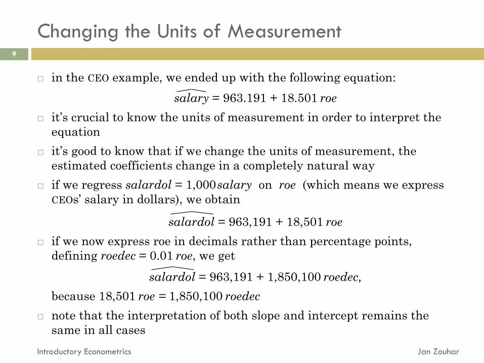
in the CEO example, we ended up with the following equation:

salary = 963.191 + 18.501 roe

it’s crucial to know the units of measurement in order to interpret the

equation

it’s good to know that if we change the units of measurement, the

estimated coefficients change in a completely natural way

if we regress salardol = 1,000salary on roe (which means we express

CEOs’ salary in dollars), we obtain

salardol = 963,191 + 18,501 roe

if we now express roe in decimals rather than percentage points,

defining roedec = 0.01 roe, we get

salardol = 963,191 + 1,850,100 roedec,

because 18,501 roe = 1,850,100 roedec

note that the interpretation of both slope and intercept remains the

same in all cases

Linear in parameters Non-linear in parameters

Functional Form


10

so far, we have only dealt with a linear relationship between x and y

this is really not as strong an assumption as you might think because we

can pick x and y to be whatever we want

as we’ve seen, changing the units doesn’t change anything; however, we

can pick a non-linear unit transform

example: E[ log(wage) | educ ] = β0 + β1 educ

E[ y | x ] = β0 + β1 x 1

→ this is still considered to be a linear regression model; the word linear

actually means linear in parameters

10

0

1

y x

yx

20 1 2

0 1log log

y x x

y x

Functional Form (cont’d)


11

which one of the following types of relationships seems more plausible:

with each additional year of education, a person’s monthly wage

increases by €50

with each additional year of education, a person’s monthly wage

increases by 5%

“5% each year” means:

if we denote E[wage|educ = 0] as w, then

E[wage|educ = 1] = w×1.05

E[wage|educ = 2] = w×1.052

E[wage|educ = 3] = w×1.053

……

E[wage|educ] = w×1.05educ

let’s generalize this type of relationship with parameters β0 and β1

1e0e

this brings us to the relationship E[wage|educ] = exp(β0 + β1 educ)

let’s focus on the meaning of β1 now

in the five-percent-a-year example, we had exp(β1) = 1.05

for β1 , this gives us , thus

this can be generalized: for a small β1, it holds

therefore, β1 tells us the (expected) percentage change in wage with

an additional year of education

0.049 0.051.05 e e



12

111 e

-1 0 1

0

1

2

1+1

exp(1)

β1

β1 exp(β1) %Δwage

0.02 1.020 2.0%

0.05 1.051 5.1%

0.20 1.221 22.1%

0.50 1.648 64.8%

1 0.05



13

note that wage = exp(β0 + β1 educ) ↔ log(wage) = β0 + β1 educ

logarithm transform is one of the basic econometric tools

the rule to remember: taking the log of one of the variables means we

shift from absolute changes to relative changes:

constant elasticity model: log y = β0 + β1 log x + u

x-elasticity of y:

regression function interpretation of β1

y = β0 + β1x Δy = β1Δx

log y = β0 + β1x %Δy = (100 β1) Δx

y = β0 + β1log x Δy = (0.01 β1) %Δx

log y = β0 + β1log x %Δy = β1%Δx

log %1 , log %

y y yxy x x x y x

E

Model 1: OLS, using observations 1-209

Dependent variable: salary

coefficient std. error t-ratio p-value

--------------------------------------------------------

const 963.191 213.240 4.517 1.05e-05 ***

roe 18.5012 11.1233 1.663 0.0978 *

Mean dependent var 1281.120 S.D. dependent var 1372.345

Sum squared resid 3.87e+08 S.E. of regression 1366.555

R-squared 0.013189 Adjusted R-squared 0.008421

F(1, 207) 2.766532 P-value(F) 0.097768

Log-likelihood -1804.543 Akaike criterion 3613.087

Schwarz criterion 3619.771 Hannan-Quinn 3615.789

SSR

Gretl Output: An Overview


14

sd 11

( )n

y SST

2 1SSE SSR

RSST SST

11

ˆn k

SSR

0 1ˆ ˆ,

1in

y y

OLS estimates as realizations of random

variables.

Mean and variance of the OLS estimator.

Classical Linear Regression

Jan Zouhar

15


A Note on Where We’re Heading…


16

as you’ve seen, we’ve only covered a small part of the Gretl output yet

gradually, we’ll build up the theory behind the following parts:

all of this tells us something about hypotheses tests about the β ’s

(this is important for empirical verification of economic theories)

Model 1: OLS, using observations 1-209

Dependent variable: salary

coefficient std. error t-ratio p-value

--------------------------------------------------------

const 963.191 213.240 4.517 1.05e-05 ***

roe 18.5012 11.1233 1.663 0.0978 *

Mean dependent var 1281.120 S.D. dependent var 1372.345

Sum squared resid 3.87e+08 S.E. of regression 1366.555

R-squared 0.013189 Adjusted R-squared 0.008421

F(1, 207) 2.766532 P-value(F) 0.097768

Log-likelihood -1804.543 Akaike criterion 3613.087

Schwarz criterion 3619.771 Hannan-Quinn 3615.789

OLS Estimator as a Random Variable


17

in our previous discussion, we always tried to estimate a population

regression function based on a (random) sample of the population

we believe there are real (population) values of β0 and β1 out there

however, we always end up with only their estimates β0 and β1

the value of these estimates depends on the specific sample we get the

data for → if we go and collect another sample, we’ll have different

estimates

→ because of random sampling, β0 and β1 can be treated as random

variables; the eventual values that we obtain are their realizations

note the difference between estimators (the RVs) and estimates

(eventual values)

it’s quite natural to ask questions like:

are my estimates accurate enough? What level of imprecision should I

count with?

is the OLS estimator unbiased? Or is it possible that, on average, the

estimates tend to overrate/underrate the intercept/slope?

îy îy

îy îy

Jan ZouharIntroductory Econometrics18

Wages vs. height in a (fictitious) population – complete data


Population regression function


Typically, we only know one sample


SRF vs PRF

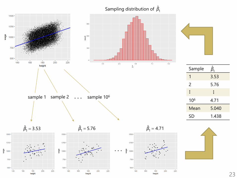
. . .sample 1 sample 2 sample 106

. . .

1ˆ 3.53β 1

ˆ 5.76β 1ˆ 4.71β

Sample

1 3.53

2 5.76

106 4.71

Mean 5.040

SD 1.438

1β

... ...

Sampling distribution of 1β

23

OLS Estimator as a Random Variable (cont’d)


26

if we translate these questions into the RV framework, we’ll be asking

about the variance and mean of β0 and β1

so far, it hasn’t really made a difference whether we took the descriptive,

causal or predictive approach

the estimates were the same, and so were their algebraic properties

the discussion about units and functional form were not related to all

of this

the goodness of fit wasn’t either

in order to say something about the properties of RVs β0 and β1, we need

to make some assumptions about the population and the sample

these will be mostly in line with the causal model

(note that the causal model was the one with the most assumptions)

e.g., the simple descriptive approach doesn’t really work with the

respective part of the Gretl output (!)

the set of assumptions (SLR.1 through SLR.6) we’ll introduce is often

referred to as the classical linear regression model (CLRM)

îy îy

îy îy

Assumptions of CLRM


27

we’ll introduce assumptions SLR.1 to SLR.4

(“SLR” stands for simple linear regression)

notice that in making this assumption we have really moved to the

“structural world”

we are really saying that this is the actual data-generating process

and our goal is to uncover the true parameters

Assumption SLR.1 (linear population model) :

In the population model, the dependent variable y is related to the

independent variable x and the error (or disturbance) u as

y = β0 + β1x + u

where β0 and β1 are the population intercept and slope

parameters, respectively.

Assumptions of CLRM (cont’d)


28

not all cross-sectional samples can be viewed as outcomes of random

samples, but many can be

with time series, we’ll have to put things differently

the next assumption effectively allows us to estimate the model

Assumption SLR.2 (random sampling):

We have a random sample of size n, (xi , yi ), i = 1,…, n

following the population model defined in SLR.1.

Assumption SLR.3 (sample variation in the explanatory variable):

The sample outcomes on x, namely {xi , i = 1,…, n}, are not all

the same value.



29

technically, the denominator for β1 is , which would be zero

if SLR.3 didn’t hold

in other words, how would you estimate the slope here:

note: in practical applications, SLR.3 always holds

educ

wage

13

21( )n

ii x x ˆiy



30

as you know, this assumption is the crucial one for causal interpretation;

at the same time, we need it in order to derive the theoretical properties

of the OLS estimator

as I’ve already noted, we make this assumption without being able to

check it by statistical means

therefore, in applications, its validity has to be argued from outside

(economic theories, common sense)

in practice, this means we have to rule out the y → x and y ← z → x

causation schemes (see lecture 2 for more details)

note that for our random sample, SLR.4 implies E[ui|x1,…,xn] = 0

we’ll use the shorthand notation x for x1,…,xn (e.g., E[ui|x] = 0)

Assumption SLR.4 (zero conditional mean of u):

The error u has an expected value of zero given any value of

the explanatory variable. In other words, E[u|x] = 0.

Mean of the OLS Estimator


31

you already know that under the assumption of random sampling

(SLR.2), β0 and β1 can be treated as RVs

our goal now is to find and

a short preview:

somehow, we want to use the assumption that E[u|x] = 0

this, however, can apply only when speaking about conditional

expectations of the estimates

therefore, we’ll first learn something about and

then we’ll use the law of iterated expectations (see our Exercise 1.13b

or Wooldridge, page 687) which tells us

we’ll start with

in order to use the assumption above, we need to express using u

ˆiy ˆiy

1E0E

x0ˆ[ | ]E E 1

ˆ[ | ] x

x

x

0 0

1 1

ˆ ˆ[ | ]

ˆ ˆ[ | ]

E E E

E E E

1

1

A Note on the Law of Iterated Expectations


32

an analogy to the following population problem

for simplicity, education classified into three categories

the average wage in the population:

500 × .20 + 700 × .50 + 800 × .30

or, in words, the weighted average, E(⋅), of the average wage in

individual categories, E[wage|educ]

E E E( ) [ | ]wage wage educ

education low medium high

average wage 500 700 800

% of the population 20 50 30

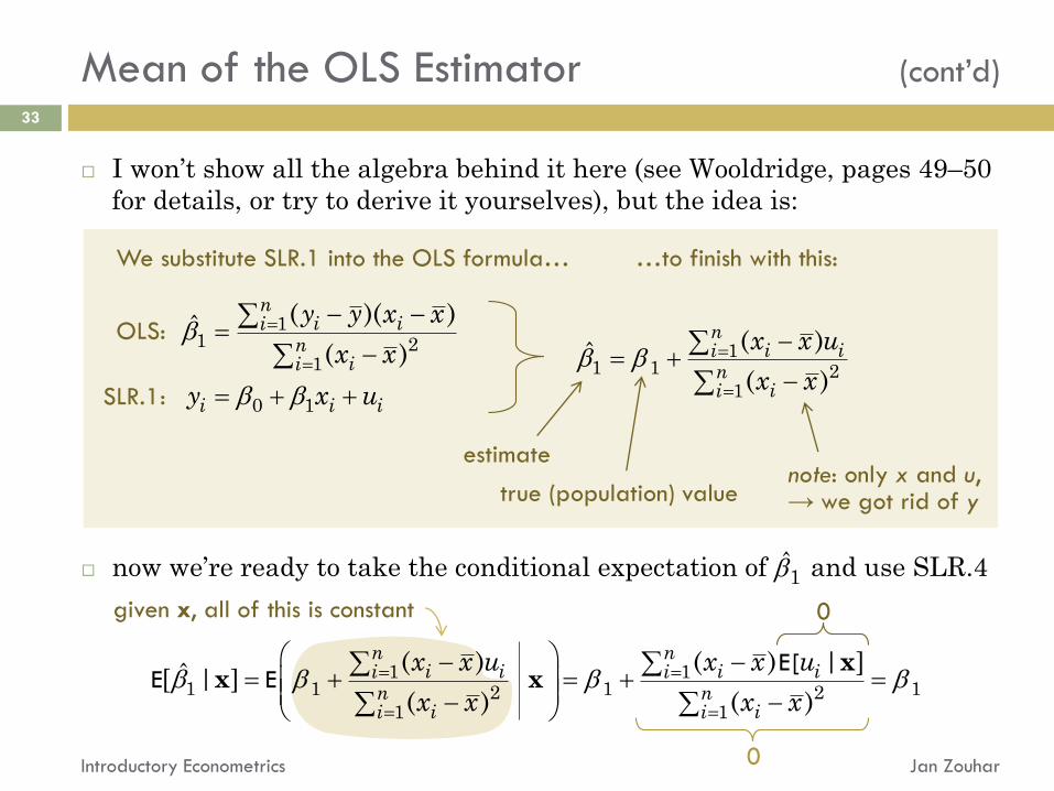
I won’t show all the algebra behind it here (see Wooldridge, pages 49–50

for details, or try to derive it yourselves), but the idea is:

now we’re ready to take the conditional expectation of and use SLR.4

xx x1 1

1 1 1 12 21 1

( ) ( ) | ]ˆ[ | ]( ) ( )

n ni i i ii i

n ni ii i

x x u x x u

x x x x

E[E E

Mean of the OLS Estimator (cont’d)


33

11 2

1

0 1

( )( )ˆ( )

ni ii

nii

i i i

y y x x

x x

y x u

11 1 2

1

( )ˆ( )

ni ii

nii

x x u

x x

estimate

true (population) valuenote: only x and u,→ we got rid of y

We substitute SLR.1 into the OLS formula… …to finish with this:

OLS:

SLR.1:

1

0

0

given x, all of this is constant



34

we have , and the law of iterated expectations tells us

this tells us that the OLS estimator is unbiased = it doesn’t

systematically overestimate/underestimate the true parameters

obviously, unbiasedness is a nice property

however, it is only a feature of the sampling distributions of β0 and β1

which says nothing about the estimate that we obtain for a given

sample

we hope that, if the sample we obtain is somehow “typical,” then our

estimate should be “near” the population value

from here, it’s easy to show the unbiasedness of :

first, note that (just averaging across the sample)

therefore,

and finally

x1 1ˆ[ | ] E

x1 1 1 1ˆ ˆ[ ] [ | ] ( ) E E E E

ˆˆ

0

0 1y x u

0 0 1 1 0 1 1 0

00

ˆ ˆ ˆ( ) ] ( )x u x u E E[ E E E

0 1 0 1 1ˆ ˆ ˆ( )y x x u OLS



35

revision: what did we need to show unbiasedness?

we started with SLR.1 and the OLS formula to get

note that in here, SLR.3 was implicitly used (no SLR.3, no slope)

then we needed SLR.2 and SLR.4:

…and finally we used the law of iterated expectations

→ to sum up, we needed all four SLR assumptions

even though one can sometimes doubt the validity of SLR.1 (linear

population relationship) or SLR.2 (true random sampling), SLR.4 is

typically the most the problematic one

11 1 2

1

( )ˆ( )

ni ii

nii

x x u

x x

SLR.4 + SLR.2

E[u|x] = 0

OLS + SLR.1

randomsampling

x1 1ˆ[ | ] Ex[ | ] 0iu E

Example: Math Performance Vs. Lunch Program


36

suppose we wish to estimate the effect of the federally funded school

lunch program on student performance. If anything, we expect the lunch

program to have a positive ceteris paribus effect on performance: all

other factors being equal, if a student who is too poor to eat regular

meals becomes eligible for the school lunch program, his or her

performance should improve.

math10 the percentage of tenth graders at a high school receiving

a passing score on a standardized mathematics exam

lnchprg the percentage of students who are eligible for the lunch

program

1. Open the lunch.gdt data file and regress math10 on lnchprg.

2. Do you think the estimated effect if lunch program is causal?

3. Or, do you think that the estimate is biased? Why? Explain why one of

the SLR assumptions is violated.

4. Suppose an estimator exhibits a downward bias. Is it possible that our

eventual estimate will be higher than the population parameter?

Accuracy of OLS Estimates, Efficiency


38

so far, we have only dealt with the mean value of our estimates

we know that with OLS there’s no bias, which means that on average,

OLS doesn’t overestimate/underestimate the true parameters

it’s good to know what happens on average, but normally we’re only

given one shot

unbiasedness actually tells us nothing about the accuracy of the

estimates

a good measure of accuracy (actually, the most widely-used one) is the

variance of the estimates

if two estimates (A and B) are both unbiased, and var A < var B, then A

is taken as the better of the two (more accurate)

we can also say that A is more efficient (we’ll have a more detailed

discussion on the efficiency of estimates later on)

in order to be able to derive a nice formula for the variance of the OLS

estimator, we need to adopt one more assumption about the variance

of u

Homoskedasticity


39

as with the conditional expectation of u (SLR.4), SLR.5 implies two

things:

1. var[u|x] is constant (not varying with x)

2. var u = σ2, i.e. the unconditional variance of u is σ2

note that once we know x, the only thing that can make y change is u

(our model is y = β0 + β1x + u, so u is the only non-constant term on the

right-hand side once x is known)

therefore, we can also re-write SLR.5 as var[y|x] = σ2

this is typically easier to interpret

Assumption SLR.5 (homoskedasticity):

Variance of u does not vary with x. More precisely, var[u|x] = σ2.

Homoskedasticity (cont’d)


40

a model satisfying our assumptions might look as follows

the conditional distributions of y have the same “width” (SLR.5) and

are centered about the PRF (SLR.4), which is linear (SLR.1)

y

x1x2

x3x

PRF: E 0 1[ | ]y x x pro

b(y

|x)



41

here, SLR.5 is violated: var[y|x] changes with x

we call this heteroskedasticity

note: the remaining assumptions are still fulfilled here

y

x1x2

x3x


b(y

|x)



42

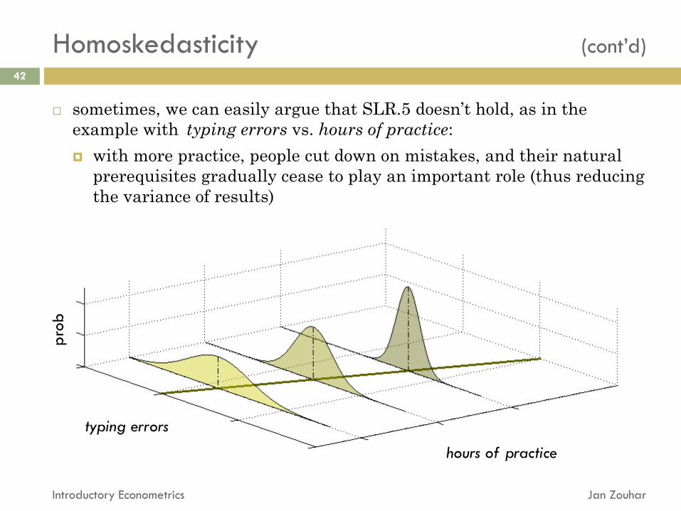
sometimes, we can easily argue that SLR.5 doesn’t hold, as in the

example with typing errors vs. hours of practice:

with more practice, people cut down on mistakes, and their natural

prerequisites gradually cease to play an important role (thus reducing

the variance of results)

typing errors

hours of practice

pro

b

Variance of the OLS Estimator


43

revision of the rules for variance calculations:

var(3u + 4) = 32 var u

var[Σui] = Σ var ui if ui are independent (for us, this is true

because of random sampling – SLR.2)

these rules apply to conditional variance as well

when we derived the mean of the OLS estimator, we used the following:

in order to simplify notation, we define , thus

note that SLR.5 and random sampling give us var[ui|x] = σ2

we can also write var[(xi – x )ui|x] = (xi – x )2σ2, because conditional on x,

(xi – x ) can be treated as a constant

11 1 2

1

( )ˆ( )

ni ii

nii

x x u

x x

2 21( )n

x iis x x

11 1 2

( )ˆn

i ii

x

x x u

s

–

–

–

Variance of the OLS Estimator (cont’d)


44

var 1ˆ[ | ] x var

var

var

11 2

1

2 2

12 2

2 21

2 2

2 212 2

2

2

( )

( )

( )

[( ) | ]

( )

( )

( )

( )

( )

ni ii

x

ni ii

x

ni ii

x

nii

x

nii

x

x

x x u

s

x x u

s

x x u

s

x x

s

x x

s

s

x

x

x



45

var 1ˆ[ | ] x

= (xi – x )2σ2–

= sx2

var

var

var

11 2

1

2 2

12 2

2 21

2 2

2 212 2

2

2

( )

( )

( )

[( ) | ]

( )

( )

( )

( )

( )

ni ii

x

ni ii

x

ni ii

x

nii

x

nii

x

x

x x u

s

x x u

s

x x u

s

x x

s

x x

s

s

x

x

x



46

put together, we have:

→ as far as the accuracy of is concerned…

…the less variance in the disturbances, the better

…the more variance in the explanatory variable, the better

on the meaning of conditional on x:

it’s the same as treating the xi as fixed in repeated samples

this is easily done in a computer simulation study

imagine we keep the x-values constant instead of generating them

at random each time, and for new samples, we generate u only

running the trials this way tells us something about the conditional

distribution of

var2

1 21

ˆ[ | ]( )nii x x

x

the variance of u

the sample variance

of x (times n – 1)

1

1

Estimating the Error Variance (σ2)


47

first note that as Eu = 0, it holds var u = Eu2

therefore, in our sample, is an unbiased estimator of var u = σ2

unfortunately, in practical applications this is useless, as we don’t know

the ui’s

instead of random errors, we’ll use the residuals (which we do know)

however, is not an unbiased estimator of σ2

the reason is that the residuals are not independent: we know that

therefore, if I tell you the first n – 2 residuals, you can tell me the

values of the remaining two (by solving the equations above)

it can be shown (see the Wooldridge book) that an unbiased estimator is

211

niinu

21 11 ˆ

niin nu SSR

1

1

0ˆ

0ˆ

nii

ni ii

u

x u

2 2112 2

ˆ ˆn SSRiin nu

Standard Errors of OLS Estimates


48

in the formula for , we needed σ2 in order to calculate the

conditional variance

once we have estimated the error variance, we can use it to estimate the

variance of the OLS estimator based on our sample

we’ll work with standard deviations rather than variances

the standard deviation of is the square root of its variance:

if we replace σ2 with estimate , we’ll obtain an estimate of ,

which is called the standard error of

var 1ˆ[ | ] x

1

sd2

1 2ˆ( )

( )ix x

se2

1 2

ˆˆ( )( )ix x

sd 1ˆ( )1

1

so far, we’ve discussed the basic characteristics of the OLS estimator

if we need to test hypotheses about the parameter values, we need to

know more than this: we need to know the sample distribution of the

OLS estimator

recall that in hypothesis testing, we use pictures like this

as you’ve seen in the simulation exercises, the OLS estimates have a

distribution that “looks somewhat like the normal distribution”

Sampling Distribution of the OLS Estimator


49

2.5% 2.5%

Sampling Distribution of the OLS Estimator (cont’d)


50

the frequency plot for the „wage vs. height“ example was:



51

there is a clear tendency towards normality: this obviously has

something to do with the central limit theorem (CLT)

the word “tendency” is related to the size of our sample here

for the CLT to take effect, we need many observations; the more

observations, the closer we are to normality

unfortunately, econometricians do not agree on a “safe” number of

observations (recommendations vary from 30 to hundreds)

in our exercise, 15 was already pretty good, but this depends on many

things

we’ll state a theorem about asymptotic normality of the OLS estimator

this theorem can put in many different versions (see Wooldridge, page

168)

the version I’ll show you is the easiest one to write down, and the most

useful in calculations

it works with standardized (or “Studentized”) estimates: se

ˆ

ˆ( )

j j

j



52

we can use this theorem to carry out hypothesis tests about β’s in case

our sample is large enough (but, what does “large enough” mean, eh?)

with a small sample, the theorem is rather useless; however, we can give

precise results here if we introduce another assumption:

Theorem: Asymptotic normality of the OLS estimator

Under the assumptions SLR.1 through SLR.5, as the sample size

increases, the distributions of standardized estimates converge towards

the standard normal distribution Normal(0,1).

Assumption SLR.6 (normality):

The population error u is independent of the explanatory variable and

is normally distributed with zero mean and variance σ2 :

u ~ Normal(0, σ2).



53

SLR.6 is much stronger than any of our previous assumptions

it actually implies both SLR.4 and SLR.5 (why?)

a succinct way to put the population assumptions (all but SLR.2) is:

y|x ~ Normal(β0 + β1 x, σ2)

y

x1x2

x3x


b(y

|x)

identical normal distributions



54

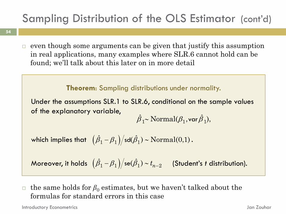
even though some arguments can be given that justify this assumption

in real applications, many examples where SLR.6 cannot hold can be

found; we’ll talk about this later on in more detail

the same holds for β0 estimates, but we haven’t talked about the

formulas for standard errors in this case

Theorem: Sampling distributions under normality.

Under the assumptions SLR.1 to SLR.6, conditional on the sample values

of the explanatory variable,

which implies that .

Moreover, it holds (Student’s t distribution).

sd1 1 1ˆ ˆ( ) Normal(0,1)

var1 1 1ˆ ˆNormal( , ),

se1 1 1 2ˆ ˆ( ) nt

Omitted Variable Bias: A Case for Multiple Regression


55

imagine we’re regressing y on x, even though there’s a substantial role of

the y ← z → x relationship

in ignoring z, we basically omitted an important variable from our

considerations

for the reasons we discussed earlier, SLR assumptions of model

y = β0 + β1x + u result in the following causal picture:

however, if there’s the y ← z → x influence, then necessarily u contains

z, and is therefore correlated with x

therefore, in the picture above

u

xy no correlation

between x and u

(SLR.4)

therefore, the correct version of our picture is

which already is a problem

a more precise picture should contain z

here, the connection between x and y leads through two paths: x → y

(direct influence) and x ← z → y (indirect influence)

Omitted Variable Bias (cont’d)


56

z

xy

u’

u

xyx and u

are correlated

u’ represents whatever is left in u

after we pull z out of it. We

assume here that u’ is correlated

with neither x nor z.

all of this was

u before



57

if we estimate the CLRM model y = β0 + β1x + u (despite knowing that the

SLR assumptions are not satisfied), the estimate of β1 captures both the

direct and indirect influence

therefore, is not unbiased anymore!

in fact, one can show that…

fortunately, there’s an easy way out of this problem: multiple regression

it suffices to estimate y = β0 + β1x + β2z + u instead (next lecture)

E corr corr1 1ˆ ( , ) ( , )

y

x

x z z y

omitted variable bias

indirect influence x ← z → y scaling factor

direct influence x → y

1



58

corr(x,z) corr(z,y) OVB

+ + +

+ – –

– + –

– – +

LECTURE 3:

SIMPLE REGRESSION II

Introductory EconometricsJan Zouhar

LECTURE 3: S R II

Documents

Transcript of LECTURE 3: S R II