Lecture 3 Probability and Measurement Error, Part 2.
65
Lecture 3 Probability and Measurement Error, Part 2
-
Upload
katherine-kennedy -
Category
Documents
-
view
236 -
download
3
Transcript of Lecture 3 Probability and Measurement Error, Part 2.

Lecture 3
Probability and Measurement Error, Part 2

SyllabusLecture 01 Describing Inverse ProblemsLecture 02 Probability and Measurement Error, Part 1Lecture 03 Probability and Measurement Error, Part 2 Lecture 04 The L2 Norm and Simple Least SquaresLecture 05 A Priori Information and Weighted Least SquaredLecture 06 Resolution and Generalized InversesLecture 07 Backus-Gilbert Inverse and the Trade Off of Resolution and VarianceLecture 08 The Principle of Maximum LikelihoodLecture 09 Inexact TheoriesLecture 10 Nonuniqueness and Localized AveragesLecture 11 Vector Spaces and Singular Value DecompositionLecture 12 Equality and Inequality ConstraintsLecture 13 L1 , L∞ Norm Problems and Linear ProgrammingLecture 14 Nonlinear Problems: Grid and Monte Carlo Searches Lecture 15 Nonlinear Problems: Newton’s Method Lecture 16 Nonlinear Problems: Simulated Annealing and Bootstrap Confidence Intervals Lecture 17 Factor AnalysisLecture 18 Varimax Factors, Empircal Orthogonal FunctionsLecture 19 Backus-Gilbert Theory for Continuous Problems; Radon’s ProblemLecture 20 Linear Operators and Their AdjointsLecture 21 Fréchet DerivativesLecture 22 Exemplary Inverse Problems, incl. Filter DesignLecture 23 Exemplary Inverse Problems, incl. Earthquake LocationLecture 24 Exemplary Inverse Problems, incl. Vibrational Problems

Purpose of the Lecture
review key points from last lecture
introduce conditional p.d.f.’s and Bayes theorem
discuss confidence intervals
explore ways to compute realizations of random variables

Part 1
review of the last lecture

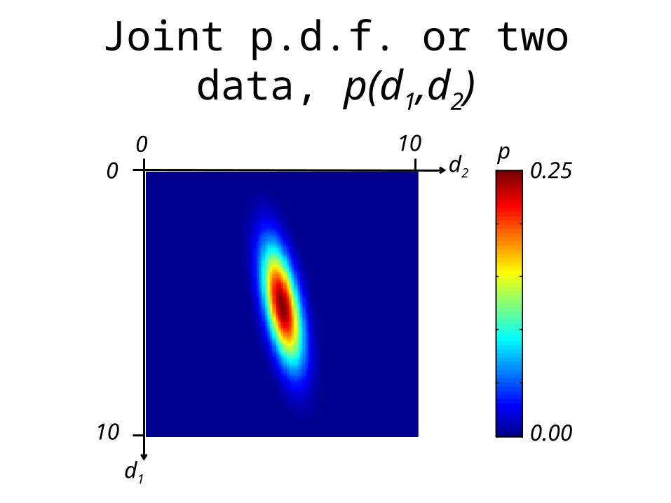
Joint probability density functions
p(d) =p(d1,d2,d3,d4…dN)probability that the data are near d
p(m) =p(m1,m2,m3,m4…mM)probability that the model parameters are near m
0
0.1
0.2
0.3
0.4
0.5
0.6
0.7
0.8
0.9
1
0
0.2
0.4
0.6
0.8
1
d1
d20 100
10 0.00
0.25pJoint p.d.f. or two data, p(d1,d2)

0
0.1
0.2
0.3
0.4
0.5
0.6
0.7
0.8
0.9
1
0
0.2
0.4
0.6
0.8
1
d1
d20 100
10 0.00
0.25p
<d1 >
<d2 >means <d1> and <d2>
0
0.1
0.2
0.3
0.4
0.5
0.6
0.7
0.8
0.9
1
0
0.2
0.4
0.6
0.8
1
d1
d20 100
10 0.00
0.25p
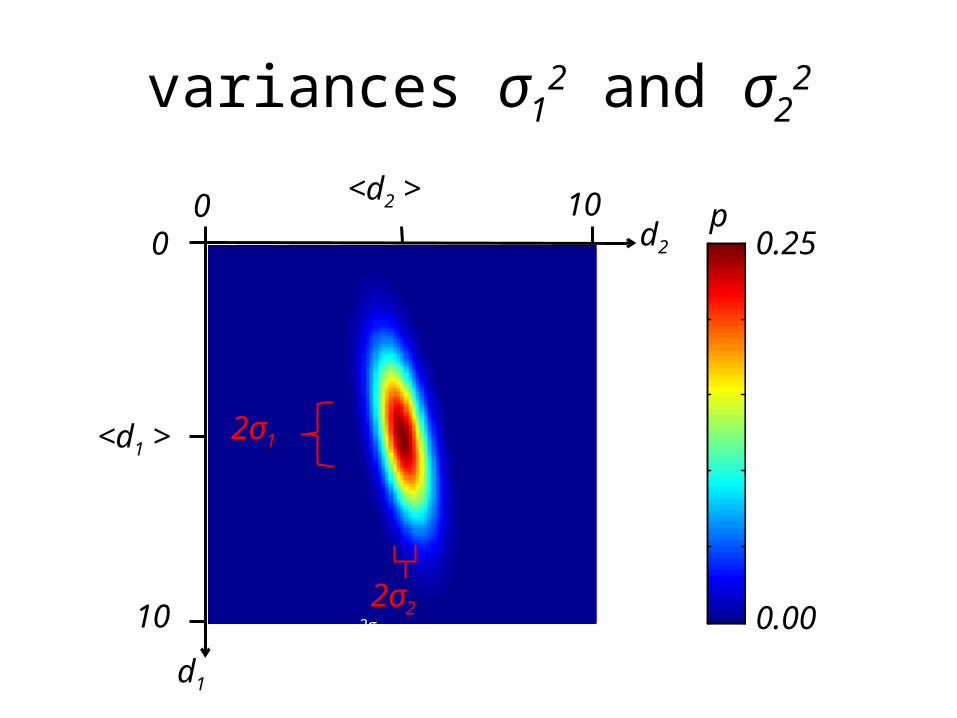
2σ1
2σ12σ2
<d1 >
<d2 >variances σ12 and σ22

0
0.1
0.2
0.3
0.4
0.5
0.6
0.7
0.8
0.9
1
0
0.2
0.4
0.6
0.8
1
d1
d20 100
10 0.00
0.25p
2σ1
2σ12σ2
θ<d1 >
<d2 >covariance – degree of correlation

summarizing a joint p.d.f.mean is a vector
covariance is a symmetric matrix
diagonal elements: variancesoff-diagonal elements: covariances

data with measurement
error
data analysis process
inferences with
uncertainty
error in measurementimplies
uncertainty in inferences

functions of random variables
given p(d)with m=f(d)
what is p(m) ?

given p(d) and m(d)then
det ∂d1/∂m1 ∂d1/∂m2 …∂d2/∂m1 ∂d2/∂m2 …………
Jacobian determinant

multivariate Gaussian example
N data, dGaussian p.d.f.
m=Md+vlinear relationship
M=N model parameters, m

given
and the linear relationm=Md+vwhat’s p(m) ?

answer
with

answer
withalso Gaussian
rule for error propagation
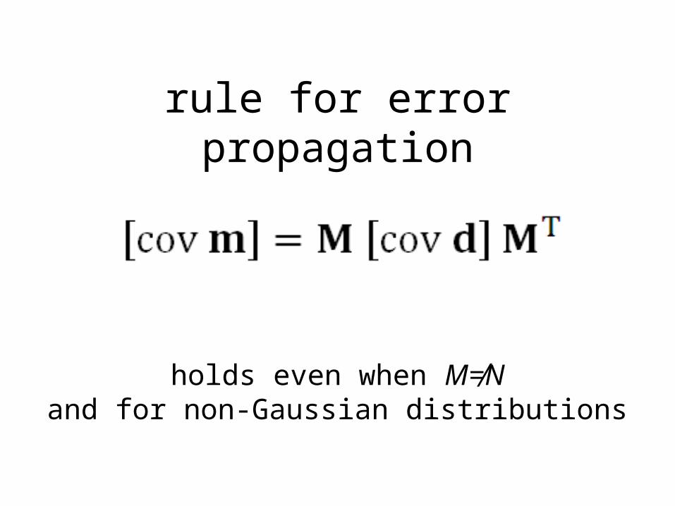
rule for error propagation
holds even when M≠Nand for non-Gaussian distributions

rule for error propagation
holds even when M≠Nand for non-Gaussian distributions
memorize

example
givengiven N uncorrelated Gaussian data with
uniform variance σd2and formula for sample mean
i

[cov d ] = σd2 I and
[cov m ] = σd2 MMT = σd2 N/N2 = (σd2 /N)I = σm2 Iorσm2 = (σd2 /N)

σm= σd /√N
so
error of sample meandecreases with number of data
decrease is rather slow , though, because of the square root

Part 2
conditional p.d.f.’s and Bayes theorem
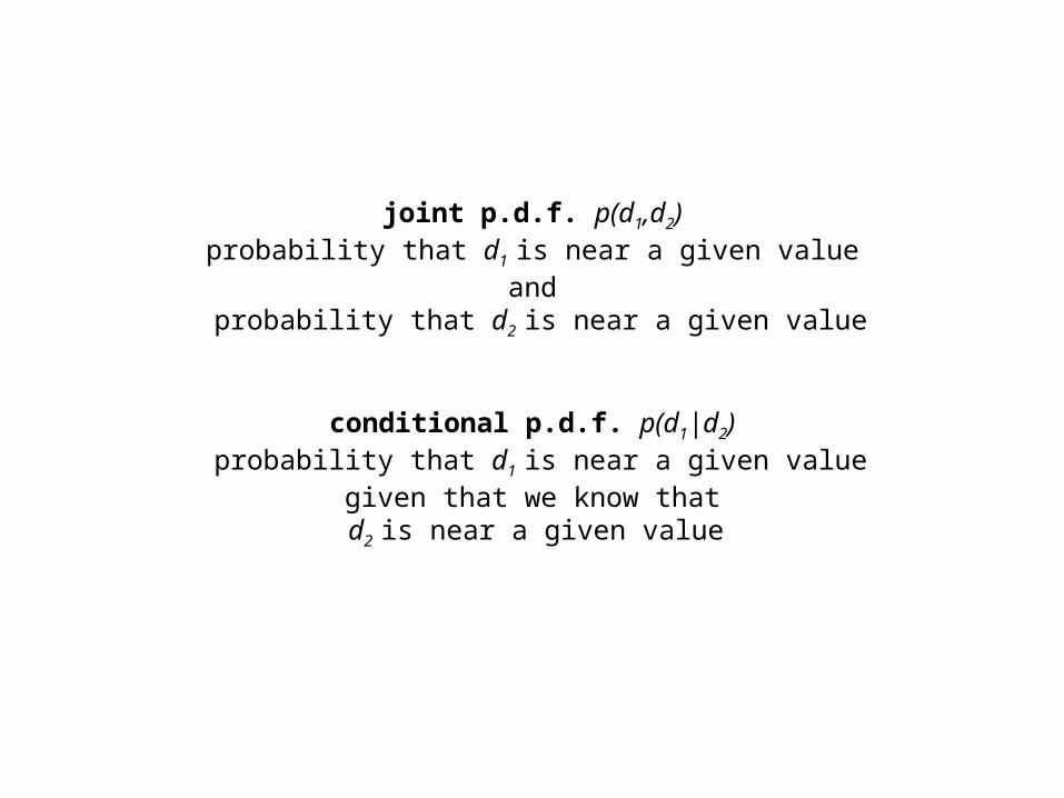
joint p.d.f. p(d1,d2)probability that d1 is near a given value
and probability that d2 is near a given value
conditional p.d.f. p(d1|d2) probability that d1 is near a given value
given that we know that d2 is near a given value

00.1
0.2
0.3
0.4
0.5
0.6
0.7
0.8
0.9
1
0
0.2
0.4
0.6
0.8
1
d1
d20 100
10 0.00
0.25pJoint p.d.f.

00.1
0.2
0.3
0.4
0.5
0.6
0.7
0.8
0.9
1
0
0.2
0.4
0.6
0.8
1
d1
d20 100
10 0.00
0.25p
2σ1
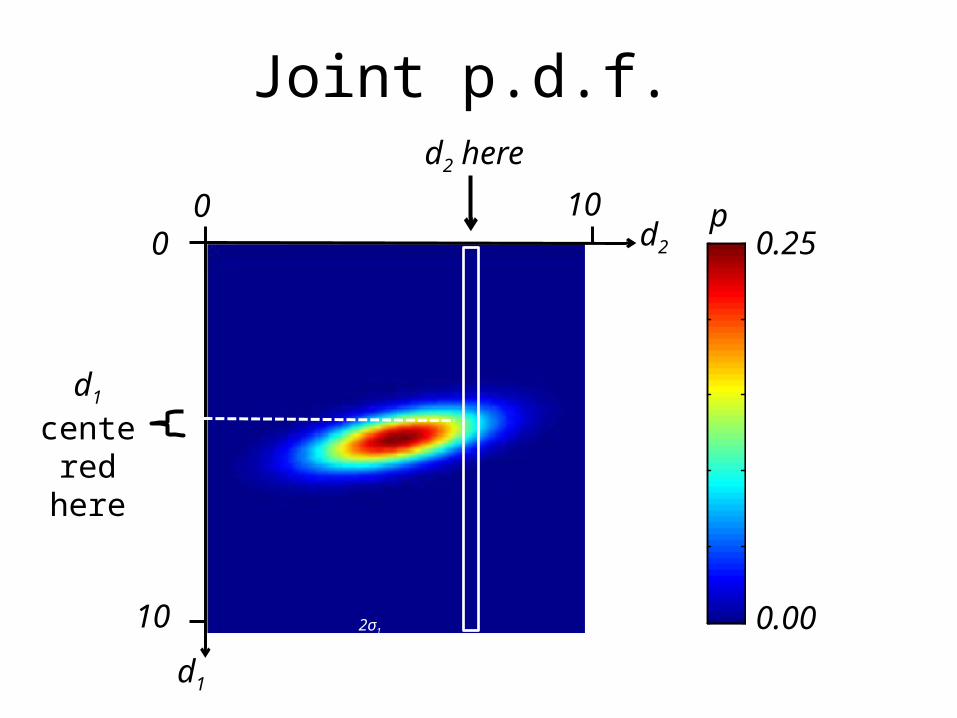
Joint p.d.f. d2 here
d1 centered
here
00.1
0.2
0.3
0.4
0.5
0.6
0.7
0.8
0.9
1
0
0.2
0.4
0.6
0.8
1
d1
d20 100
10 0.00
0.25p
2σ1
Joint p.d.f. d2 here
d1 centered
here

so, to convert ajoint p.d.f. p(d1,d2)
to a conditional p.d.f.’s p(d1|d2)evaluate the joint p.d.f. at d2
andnormalize the result to unit area


area under p.d.f. for fixed d2


similarlyconditional p.d.f. p(d2|d1)
probability that d2 is near a given valuegiven that we know that d1 is near a given value
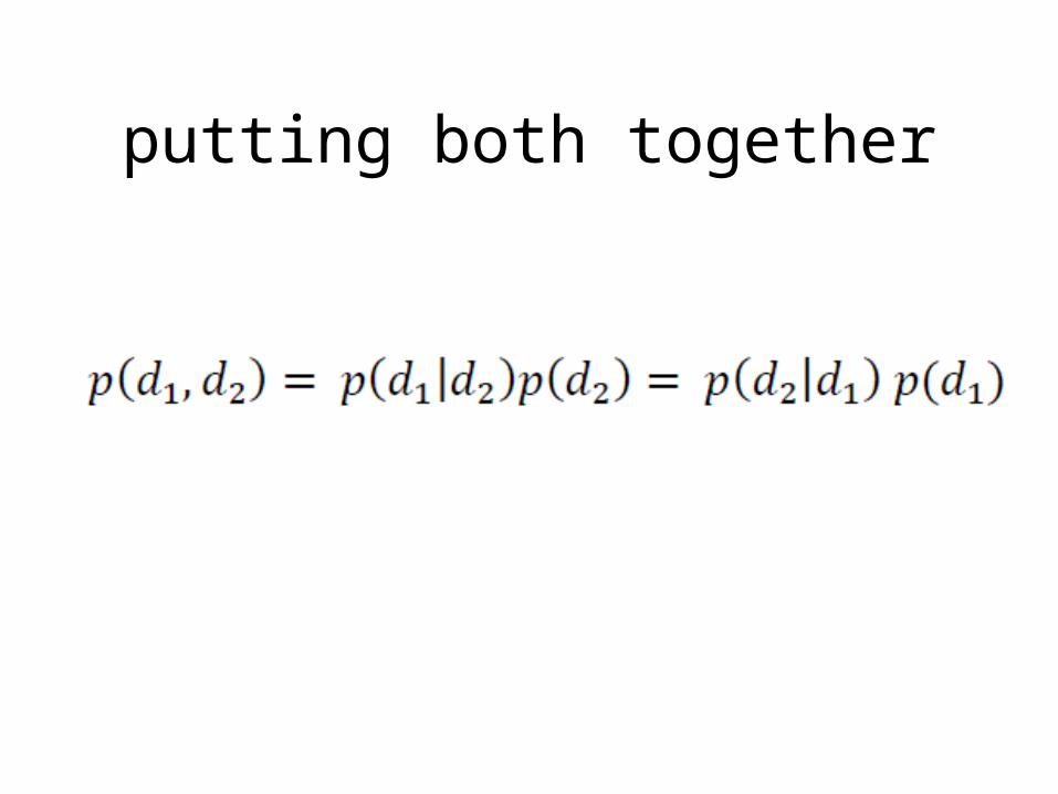
putting both together

rearranging to achieve a result calledBayes theorem

rearranging to achieve a result calledBayes theorem
three alternate ways to write p(d2)three alternate ways to write p(d1)

Importantp(d1|d2) ≠ p(d2|d1) exampleprobability that you will die given that you have pancreatic
cancer is 90%(fatality rate of pancreatic cancer is very high)
butprobability that a dead person died of pancreatic cancer is 1.3%
(most people die of something else)

Example using Sanddiscrete values
d1: grain size S=small B=Big
d2: weight L=Light H=heavy
joint p.d.f.

univariate p.d.f.’s
joint p.d.f.

univariate p.d.f.’s
joint p.d.f.
most grains are
small
most grains are
light
most grains are small and light
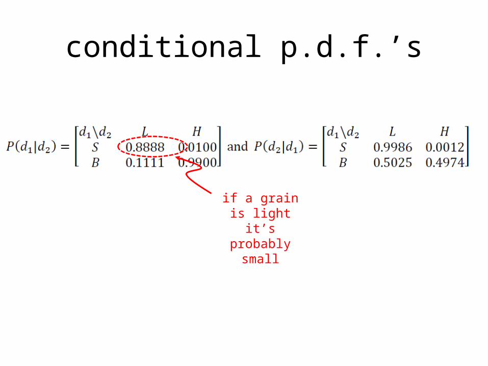
conditional p.d.f.’s
if a grain is light it’s probably
small

conditional p.d.f.’s
if a grain is heavy it’s
probably big

conditional p.d.f.’s
if a grain is small it’s probabilty
light

conditional p.d.f.’s
if a grain is big the chance is
about even that its light or heavy

If a grain is big the chance is about even that its light or heavy
?
What’s going on?

Bayes theoremprovides the answer
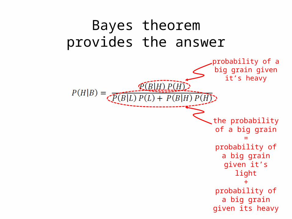
Bayes theoremprovides the answer
probability of a big grain given
it’s heavy
the probability of a big grain
=probability of a big
grain given it’s light
+probability of a big
grain given its heavy

Bayes theoremprovides the answer
only a few percent of light grains are big
butthere are a lot of light
grains
this term dominates the
result

before the observation: probability that its heavy is 10%, because heavy grains make up 10% of the total.
observation: the grain is big
after the observation: probability that the grain is heavy has risen to 49.74%
Bayesian Inferenceuse observations to update probabilities

Part 2
Confidence Intervals

suppose that we encounter in the literature the result
m1 = 50 ± 2 (95%) and m2 = 30 ± 1 (95%) what does it mean?
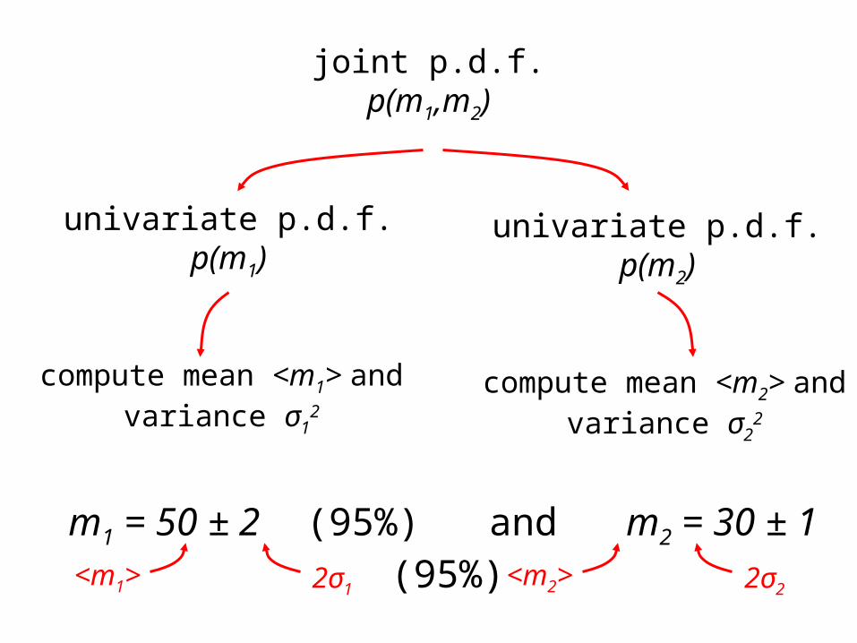
joint p.d.f.p(m1,m2)
m1 = 50 ± 2 (95%) and m2 = 30 ± 1 (95%) compute mean <m1> and
variance σ12
univariate p.d.f.p(m2)univariate p.d.f.p(m1)compute mean <m2> and
variance σ22
<m1> 2σ1 <m2> 2σ2

m1 = 50 ± 2 (95%) and m2 = 30 ± 1 (95%) irrespective of the value of m2, there is a
95% chance that m1 is between 48 and 52,
irrespective of the value of m1, there is a 95% chance that m1 is between 29 and 31,

So what’s the probability that both m1 and m2 are within 2σ of their
means?
That will depend upon the degree of correlation
For uncorrelated model parameters, it’s (0.95)2 = 0.90

0
0.1
0.2
0.3
0.4
0.5
0.6
0.7
0.8
0.9
1
m 1
m2
0
0.1
0.2
0.3
0.4
0.5
0.6
0.7
0.8
0.9
1
m 1m2
0
0.1
0.2
0.3
0.4
0.5
0.6
0.7
0.8
0.9
1
m 1
m2
m1 = <m1 >± 2σ1m2 = <m2 >± 2σ2
m1 = <m1 >± 2σ1andm2 = <m2 >± 2σ2

Suppose that you read a paper which states values and confidence
limits for 100 model parameters
What’s the probability that they all fall within their 2σ bounds?

Part 4
computing realizations of random variables

Why?
create noisy “synthetic” or “test” data
generate a suite of hypothetical models, all different from one another

MatLab function random()
can do many different p.d.f’s

But what do you do if MatLab doesn’t have the one you need?

It requires that you:1) evaluate the formula for p(d)2) already have a way to generate
realizations of Gaussian and Uniform p.d.f.’s
One possibility is to use the Metropolis-Hasting
algorithm

goal: generate a length N vector d that contains realizations of p(d)

steps:set di with i=1 to some reasonable valuenow for subsequent di+1
generate a proposed successor d’from a conditional p.d.f. q(d’|di)that returns a value near di
generate a number α from a uniformp.d.f. on the interval (0,1)
accept d’ as di+1 ifelse set di+1= di
repeat
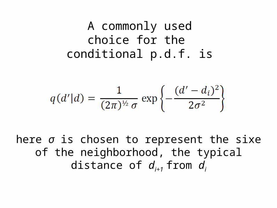
A commonly used choice for the conditional p.d.f.
is
here σ is chosen to represent the sixe of the neighborhood, the typical distance of di+1 from di

exampleexponential p.d.f.
p(d)=½c exp(-|d|/c)

-10 -5 0 5 100
0.05
0.1
0.15
0.2
0.25
0.3
d
p(d)
-10 -5 0 5 100
0.05
0.1
0.15
0.2
0.25
0.3
d
p(d)
Histogram of 5000 realizations