Lecture 3 - Probability and Bayes' rule › ... › Lectures › Lecture3.pdf · Lecture 3 -...

Lecture 3 - Probability and Bayes’ rule

DD2427

March 22, 2013

When probabilities are used

Probabilities are used to describe two quantities

• Frequencies of outcomes in random experiments.

- The probability of a coin toss landing as tails is 12 . Then if the

coin is tossed n times and kn “tails” are observed, it is

expected kn

n →12 as n→∞.

- The probability of temperature being between 10 and 11 at

midday in Stockholm during March.

• Degree of belief in propositions not involving random variables.

- the probability that Mr S. was the murderer of Mrs S. given

the evidence.

- the probability that this image contains a car given a

calculated feature vector.

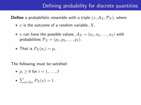
Defining probability for discrete quantities

Define a probabilistic ensemble with a triple (x,AX ,PX), where

• x is the outcome of a random variable, X,

• x can have the possible values, AX = (a1, a2, . . . , aI) withprobabilities PX = (p1, p2, . . . , pI).

• That is PX(ai) = pi.

The following must be satisfied:

• pi ≥ 0 for i = 1, . . . , I

•∑

x∈AX PX(x) = 1.

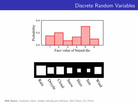
Discrete Random Variables

0.02 3 4 5 61

0.4

0.2

Face value of biased die

Pro

babi

lity

Rain

Drizzle

CloudSnow

Sleet

Sun

Wind

a) b)

0.02 3 4 5 61

0.4

0.2

Face value of biased die

Pro

babi

lity

Rain

Drizzle

CloudSnow

Sleet

Sun

Wind

a) b)

Slide Source: Computer vision: models, learning and inference. 2011 Simon J.D. Prince

A simple example

Let x be the outcome of throwing an unbiased die, then

AX = ‘1′, ‘2‘, ‘3‘, ‘4‘, ‘5‘, ‘6‘

PX =

1

6,1

6,1

6,1

6,1

6,1

6

Question:

PX(‘3‘) = ?

PX(‘5‘) = ?

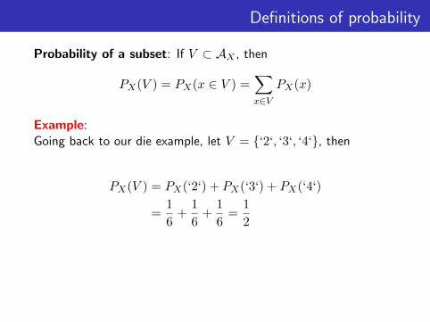
Definitions of probability

Probability of a subset: If V ⊂ AX , then

PX(V ) = PX(x ∈ V ) =∑x∈V

PX(x)

Example:Going back to our die example, let V = ‘2‘, ‘3‘, ‘4‘, then

PX(V ) = PX(‘2‘) + PX(‘3‘) + PX(‘4‘)

=1

6+

1

6+

1

6=

1

2

The simple example

Throwing an unbiased die

AX = ‘1‘, ‘2‘, ‘3‘, ‘4‘, ‘5‘, ‘6‘

PX =

1

6,1

6,1

6,1

6,1

6,1

6

Question:

If V = ‘2‘, ‘3‘, what is PX(V )?

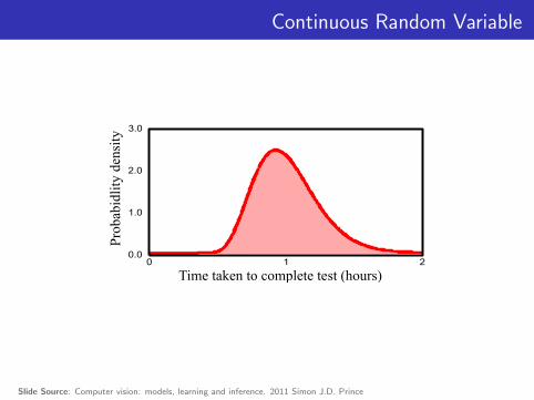
Continuous random variables

The outcome x of the random variable can also be continuous.

• In this case AX is an interval or union of intervals such asAX = (−∞,∞).

• Now pX(·) denotes the probability density function (pdf).

• It has the two properties:

1) pX(x) ≥ 0 ∀x ∈ AX ,

2)

∫x∈AX

pX(x) dx = 1.

Continuous Random Variable

0.010

2.0

1.0

Time taken to complete test (hours)

Pro

babi

dlity

den

sity

2

3.0


Continuous Random Variable

a bx

p(x)

The probability that a continuous random variable x lies betweenvalues a and b (with b > a) is defined to be

PX(a < x ≤ b) =

∫ b

x=apX(x) dx

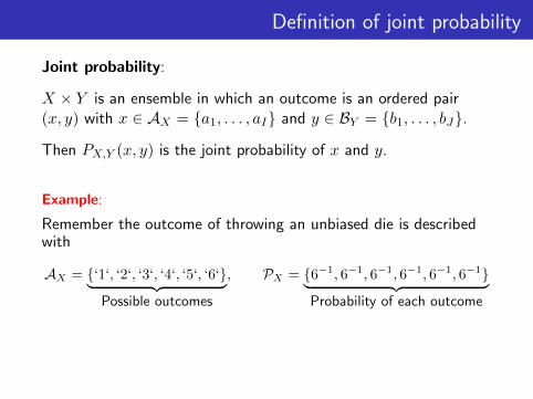
Definition of joint probability

Joint probability:

X × Y is an ensemble in which an outcome is an ordered pair(x, y) with x ∈ AX = a1, . . . , aI and y ∈ BY = b1, . . . , bJ.

Then PX,Y (x, y) is the joint probability of x and y.

Example:

Remember the outcome of throwing an unbiased die is describedwith

AX = ‘1‘, ‘2‘, ‘3‘, ‘4‘, ‘5‘, ‘6‘︸︷︷︸Possible outcomes

, PX = 6−1, 6−1, 6−1, 6−1, 6−1, 6−1︸︷︷︸Probability of each outcome

Definition of joint probability

Example ctd:

The output of two consecutive independent throws of an unbiased die:

Throw 1: AT1 = ‘1‘, ‘2‘, ‘3‘, ‘4‘, ‘5‘, ‘6‘PT1

= 6−1, 6−1, 6−1, 6−1, 6−1, 6−1

Throw 2: AT2= ‘1‘, ‘2‘, ‘3‘, ‘4‘, ‘5‘, ‘6‘

PT2 = 6−1, 6−1, 6−1, 6−1, 6−1, 6−1

Possible outcomes: AT1×T2 = (‘1‘, ‘1‘), (‘1‘, ‘2‘), (‘1‘, ‘3‘), . . . , (‘1‘, ‘6‘),

(‘2‘, ‘1‘), (‘2‘, ‘2‘), (‘2‘, ‘3‘), . . . , (‘2‘, ‘6‘),

. . . . . . . . . . . . . . . . . .(‘6‘, ‘1‘), (‘6‘, ‘2‘), (‘6‘, ‘3‘), . . . , (‘6‘, ‘6‘)

Probabilities: PT1×T2 =

136 ,

136 , · · · ,

136

Another example

Scenario:A person throws an unbiased die. If the outcome is even throwthis die again, otherwise throw a die biased towards ‘3‘ with

PX =

1

10,

1

10,1

2,

1

10,

1

10,

1

10

Questions:

What is the set, AT1×T2 , of possible outcomes?

What are the values in PT1×T2 ?

Joint Probabilitya) b) c)

d) e) f)


Joint Probability

a) b) c)

d) e) f)


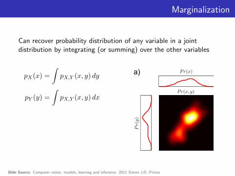
Marginalization

Can recover probability distribution of any variable in a jointdistribution by integrating (or summing) over the other variables

PX(ai) ≡∑

y∈AY

PX,Y (ai, y)

PY (bj) ≡∑

x∈AX

PX,Y (x, bj)

a) b) c)


Marginalization


pX(x) =

∫pX,Y (x, y) dy

pY (y) =

∫pX,Y (x, y) dx

a) b) c)


Marginalization


pX(x) =∑y

PX,Y (x, y)

PY (y) =

∫xPX,Y (x, y) dx

a) b) c)


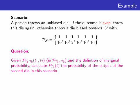
Example

Scenario:A person throws an unbiased die. If the outcome is even, throwthis die again, otherwise throw a die biased towards ‘3‘ with

PX =

1

10,

1

10,1

2,

1

10,

1

10,

1

10

Question:

Given PT1,T2(t1, t2) (ie PT1×T2) and the defintion of marginalprobability, calculate PT2(t) the probability of the output of thesecond die in this scenario.

Conditional Probability

• Conditional probability of X given Y = y1 is the relativepropensity of variable X to take different values given Y hasvalue y1.

• Written as PX|Y (x | y1).


Conditional Probability

• Conditional probability is extracted from joint probability

• Extract appropriate slice and normalize

pX|Y (x | y∗) =pX,Y (x,y∗)∫pX,Y (x,y∗) dx

=pX,Y (x,y∗)pY (y∗)


Conditional Probability (Discrete)

PX|Y (x | y∗) = PX,Y (x,y∗)∑x∈AX

PX,Y (x,y∗)=

PX,Y (x,y∗)

PY (y∗)

Example:

Revisiting our example modelling the output of two consecutiveindependent throws of an unbiased die then

PT2|T1(‘3‘ | ‘1‘) =PT1,T2(‘1‘, ‘3‘)

PT1(‘1‘)=

13616

=1

6

Example

Scenario:

A person throws an unbiased die. If the outcome is even, throwthis die again, otherwise throw a die biased towards ‘3‘ with

PX =

1

10,

1

10,1

2,

1

10,

1

10,

1

10

Question:

Calculate PT2|T1(‘3‘ | ‘1‘) and PT2|T1(‘3‘ | ‘2‘).

Rules of probability

• Product Rule: from definition of the conditional probability

PX,Y (x, y) = PX|Y (x | y)PY (y) = PY |X(y | x)PX(x)

• Sum/Chain Rule: rewriting marginal probability definition

PX(x) =∑y

PX,Y (x, y) =∑y

PX|Y (x | y)PY (y)

• Bayes’ Rule: from the product rule

PY |X(y | x) =PX|Y (x | y)PY (y)

PX(x)=

PX|Y (x | y)PY (y)∑y′ PX|Y (x | y′)PY (y′)

An Example

Problem: Jo has the test for a nasty disease. Let A be the r.v.denoting the state of Jo’s health and B the test results.

A =

1 if Jo has the disease,

0 Jo does not have the diseaseB =

1 if the test is positive,

0 if the test is negative.

The test is 95% reliable, that is

PB|A(1 | 1) = .95 PB|A(1 | 0) = .05

PB|A(0 | 1) = .05 PB|A(0 | 0) = .95

The final piece of background information is that 1% of peopleJo’s age and background have the disease.

Jo has the test and the result is positive.

What is the probability Jo has the disease?

Solution

The background information tells us

PA(1) = .01, PA(0) = .99

Jo would like to know how plausible it is that she has the disease.

This involves calculating PA|B(1 | 1) which is the probability of Johaving the disease given a positive test result.

Applying Bayes’ Rule:

PA|B(1 | 1) =PB|A(1 | 1)PA(1)

PB(1)

=PB|A(1 | 1)PA(1)

PB|A(1 | 1)PA(1) + PB|A(1 | 0)PA(0)

=.95× .01

.95× .01 + .05× .99= .16

Your Turn

Scenario: Your friend has two envelopes. One he calls the Winenvelope which has 100 dollars and four beads ( 2 red and 2 blue)in it. While the other the Lose envelope has three beads ( 1 redand 2 blue) and no money. You choose one of the envelopes atrandom and then your friend offers to sell it to you.

Question:

• How much should you pay for the envelope?

• Suppose before deciding you are allowed to draw one beadfrom the envelope.

If this bead is blue how much should you pay?

Inference is important

• Inference is the term given to the conclusions reached fromthe basis of evidence and reasoning.

• Most of this course will be devoted to inference of some form.

• Some examples:

I’ve got this evidence. What’s the chance that this conclusionis true?

- I’ve got a sore neck: How likely am I to have meningitis?

- My car detector has fired in this image: How likely is itthere is a car in the image?

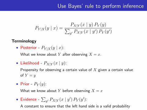
Use Bayes’ rule to perform inference

PY |X(y | x) =PX|Y (x | y)PY (y)∑y′ PX|Y (x | y′)PY (y′)

Terminology

• Posterior - PY |X(y | x):

What we know about Y after observing X = x.

• Likelihood - PX|Y (x | y):

Propensity for observing a certain value of X given a certain value

of Y = y

• Prior - PY (y):

What we know about Y before observing X = x

• Evidence -∑

y′ PX|Y (x | y′)PY (y′):

A constant to ensure that the left hand side is a valid probability

distribution

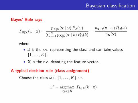
Bayesian classification

Bayes’ Rule says

PΩ|X(ω | x) =pX|Ω(x | ω)PΩ(ω)∑Kk=1 pX|Ω(x | k)PΩ(k)

=pX|Ω(x | ω)PΩ(ω)

pX(x)

where

• Ω is the r.v. representing the class and can take values1, . . . ,K.

• X is the r.v. denoting the feature vector.

A typical decision rule (class assignment)

Choose the class ω ∈ 1, . . . ,K s.t.

ω∗ = arg max1≤k≤K

PΩ|X(k | x)

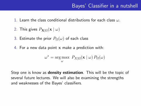
Bayes’ Classifier in a nutshell

1. Learn the class conditional distributions for each class ω.

2. This gives PX|Ω(x | ω)

3. Estimate the prior PΩ(ω) of each class

4. For a new data point x make a prediction with:

ω∗ = arg maxω

PX|Ω(x | ω)PΩ(ω)

Step one is know as density estimation. This will be the topic ofseveral future lectures. We will also be examining the strengthsand weaknesses of the Bayes’ classifiers.

Independence

If X and Y are independent then knowing that Y = y tells usnothing about variable X (and vice-versa) that is

PX|Y (x | y) = PX(x)

PY |X(y | x) = PY (y)

a) b)


Independence

If X and Y are independent then knowing that Y = y tells usnothing about variable X (and vice-versa) that is

pX|Y (x | y) = pX(x)

pY |X(y | x) = pY (y)

a) b)


Independence

When X and Y are independent then

PX,Y (x, y) = PX|Y (x | y)PY (y)

= PY |X(y | x)PX(x)

= PX(x)PY (y)

a) b)


Expectations

Expectation

Expectation tell us the average value of some function f(x) takinginto account the distribution of x.

Definition:

E [f(X)] =∑x∈AX

f(x)PX(x)

E [f(X)] =

∫x∈AX

f(x) pX(x) dx


Expectation

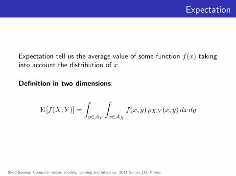
Expectation tell us the average value of some function f(x) takinginto account the distribution of x.

Definition in two dimensions:

E [f(X,Y )] =

∫y∈AY

∫x∈AX

f(x, y) pX,Y (x, y) dx dy


Expectation: Common Cases

Function f(X) Expectation

X mean, µXXk kth moment about zero(X − µX)k kth moment about the mean(X − µX)2 variance(X − µX)3 skew(X − µX)4 kurtosis(X − µX)(Y − µY ) covariance of X and Y

E [f(X)] =

∫x∈AX

f(x) pX(x) dx


Expectation: Rules

E [f(X)] =

∫x∈AX

f(x) pX(x) dx

Rule 1:

Expected value of a constant function f(X) = κ is a constant:

E [f(X)] =

∫xf(x) pX(x) dx

=

∫xκ pX(x) dx

= κ

∫xpX(x) dx

= κ


Expectation: Rules

E [f(X)] =

∫x∈AX

f(x) pX(x) dx

Rule 2:

Expected value of a function g(X) = κ f(x) then

E [g(X)] = E [κ f(X)] =

∫xκ f(x) pX(x) dx

= κ

∫xf(x) pX(x) dx

= κE [f(X)]


Expectation: Rules

E [f(X)] =

∫x∈AX

f(x) pX(x) dx

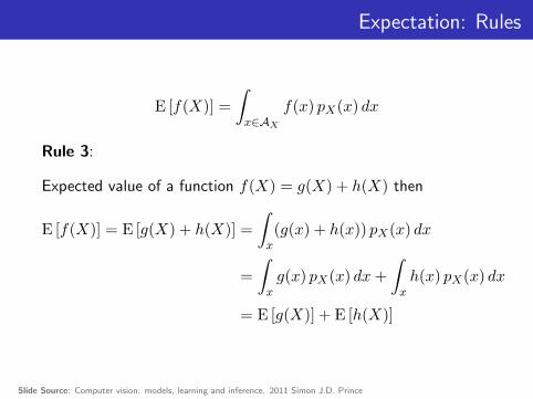
Rule 3:

Expected value of a function f(X) = g(X) + h(X) then

E [f(X)] = E [g(X) + h(X)] =

∫x(g(x) + h(x)) pX(x) dx

=

∫xg(x) pX(x) dx+

∫xh(x) pX(x) dx

= E [g(X)] + E [h(X)]


Expectation: Rules

E [f(X)] =

∫x∈AX

f(x) pX(x) dx

Rule 4:

If X and Y are independent r.v.’s the expected value of a functionf(X,Y ) = g(X)h(Y ) is

E [f(X,Y )] = E [g(X)h(Y )] =

∫y

∫xg(x)h(y) pX,Y (x, y) dx dy

=

∫y

∫xg(x)h(y) pX(x) pY (y) dx dy

=

∫xg(x) pX(x) dx

∫yh(y) pY (y) dy

= E [g(X)] E [h(Y )]


Expectation of a vector

Mean vector

E [X] = (E [X1] ,E [X2] , . . . ,E [Xp])T = (µX1 , . . . , µXp)

T = µX

Mean

Expectation of matrix

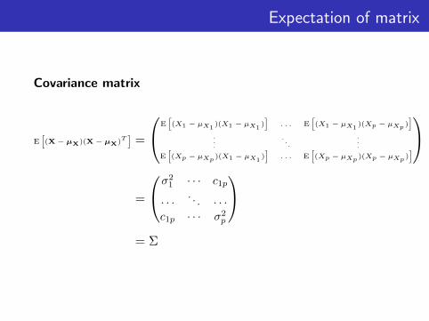
Covariance matrix

E[(X− µX)(X− µX)

T]

=

E[(X1 − µX1

)(X1 − µX1)]

. . . E[(X1 − µX1

)(Xp − µXp )]

.

.

.. . .

.

.

.

E[(Xp − µXp )(X1 − µX1

)]

. . . E[(Xp − µXp )(Xp − µXp )

]

=

σ21 · · · c1p

· · ·. . . · · ·

c1p · · · σ2p

= Σ

Covariance matrix

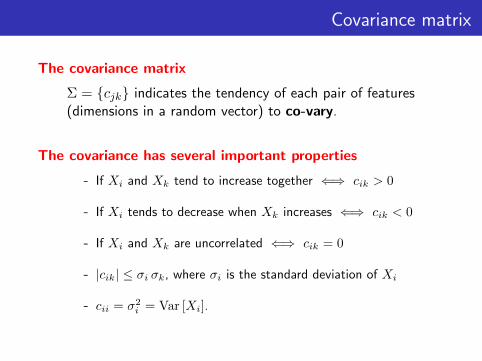
The covariance matrix

Σ = cjk indicates the tendency of each pair of features(dimensions in a random vector) to co-vary.

The covariance has several important properties

- If Xi and Xk tend to increase together ⇐⇒ cik > 0

- If Xi tends to decrease when Xk increases ⇐⇒ cik < 0

- If Xi and Xk are uncorrelated ⇐⇒ cik = 0

- |cik| ≤ σi σk, where σi is the standard deviation of Xi

- cii = σ2i = Var [Xi].

Covariance matrix

Covariance terms can be expressed as

cii = σ2i and cik = ρikσiσk

where ρik is called the correlation coefficient.

ρik = −1 ρik = − 12 ρik = 0 ρik = 1

2 ρik = 1

Introduction to Pattern AnalysisRicardo Gutierrez-OsunaTexas A&M University

17

Covariance matrix (1)! The covariance matrix indicates the tendency of each pair of features

(dimensions in a random vector) to vary together, i.e., to co-vary*! The covariance has several important properties

" If xi and xk tend to increase together, then cik>0" If xi tends to decrease when xk increases, then cik<0" If xi and xk are uncorrelated, then cik=0" |cik|!"i"k, where "i is the standard deviation of xi

" cii = "i2 = VAR(xi)

! The covariance terms can be expressed as

" where #ik is called the correlation coefficientkiikik

2iii candc ""#" $$

Xi

Xk

Cik=-"i"k#ik=-1

Xi

Xk

Cik=-½"i"k#ik=-½

Xi

Xk

Cik=0#ik=0

Xi

Xk

Cik=+½"i"k#ik=+½

Xi

Xk

Cik="i"k#ik=+1

*from http://www.engr.sjsu.edu/~knapp/HCIRODPR/PR_home.htm

Covariance matrix II

The covariance matrix can be reformulated as

Σ = E[(X− µX)(X− µX)T

]= E

[XXT

]−µXµTX = S−µXµTX

with

S = E[XXT

]=

E [X1X1] . . . E [X1Xp]... . . .

...E [XpX1] . . . E [XpXp]

S is called the auto-correlation matrix and contains the sameamount of information as the covariance matrix.


The covariance matrix can also be expressed as

Σ = ΓRΓ =

σ1 0 . . . 00 σ2 . . . 0...

.... . .

...0 0 . . . σp

1 ρ12 . . . ρ1pρ12 1 . . . ρ2p...

.... . .

...ρ1p ρ2p . . . 1

σ1 0 . . . 00 σ2 . . . 0...

.... . .

...0 0 . . . σp

• A convenient formulation since Γ contains the scales of thefeatures and R retains the essential information of therelationship between the features.

• R is the correlation matrix.


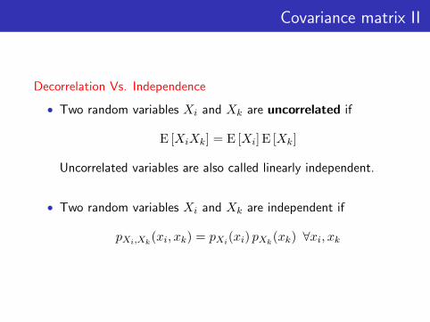
Decorrelation Vs. Independence

• Two random variables Xi and Xk are uncorrelated if

E [XiXk] = E [Xi] E [Xk]

Uncorrelated variables are also called linearly independent.

• Two random variables Xi and Xk are independent if

pXi,Xk(xi, xk) = pXi(xi) pXk(xk) ∀xi, xk

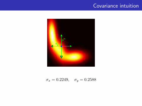
Covariance intuition

σx

σ y

σx = 0.2249, σy = 0.2588

Covariance intuition

• Eigenvectors of Σ are the orthogonal directions where there isthe most spread in the underlying distribution.

• The eigenvalues indicate the magnitude of the spread.

The Normal Distribution

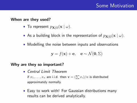
Some Motivation

When are they used?

• To represent pX|Ω(x | ω).

• As a building block in the representation of pX|Ω(x | ω).

• Modelling the noise between inputs and observations

y = f(x) + e, e ∼ N (0,Σ)

Why are they so important?

• Central Limit Theoremif x1, . . . , xn are i.i.d. then v = (

∑xi)/n is distributed

approximately normally.

• Easy to work with! For Gaussian distributions manyresults can be derived analytically.

Univariate Normal Distribution

• Univariate normal distribution is a pdf describing a continuousvariable:

pX(x) = 1√2πσ2

exp−1

2

(x−µσ

)2• Defined by 2 parameters µ and σ > 0.

(0.0,1.0)

(-3.4,0.25)

(1.5,4.41)

Prob

abili

ty D

ensi

ty

-6 60

• Will denote the Normal distribution by

N (µ, σ2)

Univariate Normal Distribution

pX(x) = 1√2πσ2

exp−1

2

(x−µσ

)2• If X ∼ N (x;µ, σ2) then

E [X] = µ

Var [X] = σ2

• Write X ∼ N (x;µ, σ2) to denote:

X is distributed Normally with mean µ and variance σ2.

The Central Limit Theorem

• Assume X1, X2, . . . , Xn are i.i.d. random variables with

E [Xi] = µ

Var [Xi] = σ2

• Define

Zn = f(X1, X2, . . . , Xn) =1

n

n∑i=1

Xi

then

pZn(z) = N (z;µ, σ2/n)

for sufficiently large n.

Illustration

• n = 1for j = 1 to 500

One sample, xj,1, is drawn from a uniform distribution.Compute and record zj =

∑ni=1 xj,i/n.


21

Central Limit Theorem! The central limit theorem states that given a distribution with a mean !

and variance "2, the sampling distribution of the mean approaches a normal distribution with a mean (!) and a variance "i

2/N as N, the sample size, increases.

" No matter what the shape of the original distribution is, the sampling distribution of the mean approaches a normal distribution

" Keep in mind that N is the sample size for each mean and not the number of samples

! A uniform distribution is used to illustrate the idea behind the Central Limit Theorem

" Five hundred experiments were performed using am uniform distribution

! For N=1, one sample was drawn from the distribution and its mean was recorded (for each of the 500 experiments)

" Obviously, the histogram shown a uniform density! For N=4, 4 samples were drawn from the

distribution and the mean of these 4 samples was recorded (for each of the 500 experiments)

" The histogram starts to show a Gaussian shape! And so on for N=7 and N=10! As N grows, the shape of the histograms resembles

a Normal distribution more closely

The histogram of the zj ’s shows a uniform density.

• n = 4for j = 1 to 500

Four samples, xj,1, . . . , xj,4, are drawn from a uniform distribution.Compute and record zj =

∑ni=1 xj,i/n.


21













The histogram of the zj ’s starts to show a Gaussian shape.

Illustration

• Similarly for n = 7


21













• Similarly for n = 10


21












a Normal distribution more closelyAs n grows the histogram increasingly resembles a Gaussian.

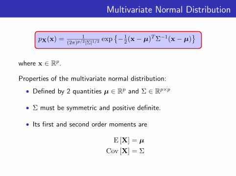
Multivariate Normal Distribution

pX(x) = 1(2π)p/2|Σ|1/2 exp

−1

2(x− µ)TΣ−1(x− µ)

where x ∈ Rp.

Properties of the multivariate normal distribution:

• Defined by 2 quantities µ ∈ Rp and Σ ∈ Rp×p

• Σ must be symmetric and positive definite.

• Its first and second order moments are

E [X] = µ

Cov [X] = Σ

General Gaussian

µ =

µ1

µ2

...µp

, Σ =

σ21 σ12 · · · σ1p

σ12 σ22 · · · σ2p

......

. . ....

σ1p σ2p · · · σ2p

−20 −15 −10 −5 0 5 10 15 20

−15

−10

−5

0

5

10

15

Axis-aligned Gaussian

µ =

µ1

µ2

...µp

, Σ =

σ21 0 · · · 0 0

0 σ22 · · · 0 0

......

. . ....

...0 0 · · · σ2

p−1 00 0 · · · 0 σ2

p

−25 −20 −15 −10 −5 0 5 10 15 20 25

−15

−10

−5

0

5

10

15

Spherical Gaussian

µ =

µ1

µ2

...µp

, Σ =

σ2 0 · · · 0 00 σ2 · · · 0 0...

.... . .

......

0 0 · · · σ2 00 0 · · · 0 σ2

−15 −10 −5 0 5 10 15−15

−10

−5

0

5

10

15

Degenerate Gaussian

µ =

µ1

µ2

...µp

, |Σ| = 0

Explicit Illustrations

5

-5

-5 5-5 5-5 5

5

-5

a ) c ) e )

b ) d ) f)

Spherical covariances Diagonal covariances Full covariances


Diagonal Covariance = Independence

• Say µ =(0 0

)Tand Σ =

(σ21 0

0 σ22

)then

pX1,X2(x1, x2) =1

2π√|Σ|

exp

−0.5

(x1 x2

)Σ−1

(x1x2

)

=1

2πσ1σ2exp

−0.5

(x1 x2

)(σ−21 00 σ−2

2

)(x1x2

)

=1

σ1

√2π

exp

− x21

2σ21

1

σ2

√2π

exp

− x22

2σ22

= pX1(x1) pX2(x2)

• Similarly can easily show

pX1,...,Xp(x1, . . . , xp) =

p∏i=1

pXp(xp)

when Σ = diag(σ21 , . . . , σ

2p)

Decomposition of the Covariance Matrix

• Say X ∼ N (x;µ,Σ)

• Assuming Σ is diagonalizable then Σ = U Σdiag U−1 where

∗ Each column of U is an eigenvector of Σ.

∗ Σdiag is a diagonal matrix whose diagonal elements are the

eigenvalues of Σ.

• Σ is symmetric =⇒ U−1 = UT =⇒ Σ = U Σdiag UT

• Therefore

pX(x) =1

2π√|Σ|

exp−0.5xTΣx

=

1

2π√|U Σdiag U−1|

exp−0.5xTU Σ−1

diag UT x

=1

2π√|U | |Σdiag| |U |−1

exp−0.5 (UTx)T Σ−1

diag (UT x), |AB| = |A||B|

=1

2π√|Σdiag|

exp−0.5x′T Σ−1

diag x′

= pX′(x′), x′= P

Tx

Decomposition of the Covariance Matrix

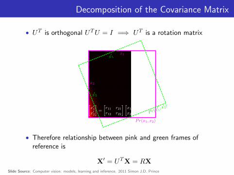
• UT is orthogonal UTU = I =⇒ UT is a rotation matrix

• Therefore relationship between pink and green frames ofreference is

X′ = UTX = RX


Transformation of Variables

b)a)

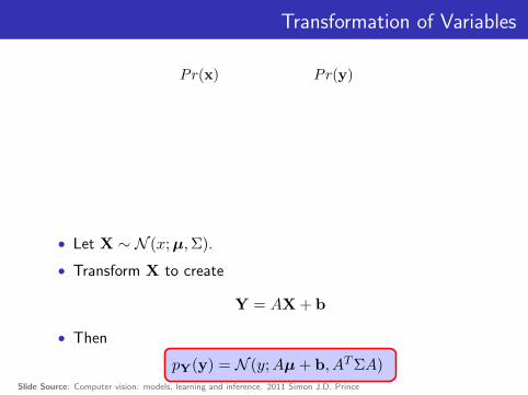
• Let X ∼ N (x;µ,Σ).

• Transform X to create

Y = AX + b

• Then

pY(y) = N (y;Aµ + b, ATΣA)Slide Source: Computer vision: models, learning and inference. 2011 Simon J.D. Prince

Marginal Distributions

• Marginal distributions of amultivariate normal are alsonormal

pX(x) = pX

((x1

x2

))= N

(x;

(µ1

µ2

),

(Σ11 ΣT21Σ21 Σ22

))• Then

pX1(x1) = N (x1;µ1,Σ11)

pX2(x2) = N (x2;µ2,Σ22)


Conditional Distributions

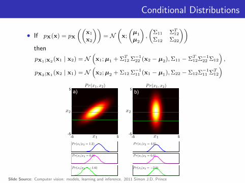
• If pX(x) = pX

((x1

x2

))= N

(x;

(µ1

µ2

),

(Σ11 ΣT12Σ12 Σ22

))then

pX1|X2(x1 | x2) = N

(x1;µ1 + ΣT12 Σ−1

22 (x2 − µ2),Σ11 − ΣT12Σ−122 Σ12

),

pX2|X1(x2 | x1) = N

(x2;µ2 + Σ12 Σ−1

11 (x1 − µ1),Σ22 − Σ12Σ−111 ΣT12

)a)

-5 5-5

5b)

-5 5-5

5


Conditional Distributions

a)

-5 5-5

5b)

-5 5-5

5

Note: For spherical / diagonal case, X1 and X2 are independentso all of the conditional distributions are the same.


Change of Variables

If

X | (Y = y) ∼ N (x; ay + b, σ2)

then

Y | (X = x) ∼ N (y; a′x+ b′, σ′2)

a) b)

0

1

0 1 0 10

1


Today’s assignment

Pen & Paper assignment

• Details available on the course website.

• You will be asked to perform some simple Bayesian reasoning.

• Mail me about any errors you spot in the Exercise notes.

• I will notify the class about errors spotted and corrections viathe course website and mailing list.

Lecture 3 - Probability and Bayes' rule › ... › Lectures › Lecture3.pdf · Lecture 3 -...

Documents

Transcript of Lecture 3 - Probability and Bayes' rule › ... › Lectures › Lecture3.pdf · Lecture 3 -...