Lecture 3 – Parallel Performance Theory - 1

Parallel Performance Theory - 1

Parallel Computing

CIS 410/510

Department of Computer and Information Science

Lecture 3 – Parallel Performance Theory - 1

Outline

• Performance scalability• Analytical performance measures• Amdahl’s law and Gustafson-Barsis’ law

2Introduction to Parallel Computing, University of Oregon, IPCC

Lecture 3 – Parallel Performance Theory - 1 3

What is Performance? In computing, performance is defined by 2 factors

❍ Computational requirements (what needs to be done)❍ Computing resources (what it costs to do it)

Computational problems translate to requirements Computing resources interplay and tradeoff

Time Energy

… and ultimately

MoneyHardware

Performance ~1

Resources for solution

Introduction to Parallel Computing, University of Oregon, IPCC

Lecture 3 – Parallel Performance Theory - 1

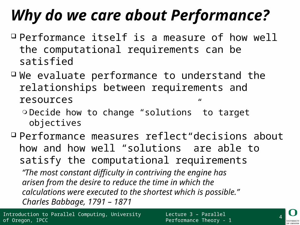
Why do we care about Performance? Performance itself is a measure of how well the

computational requirements can be satisfied We evaluate performance to understand the

relationships between requirements and resources❍ Decide how to change “solutions” to target objectives

Performance measures reflect decisions about how and how well “solutions” are able to satisfy the computational requirements

“The most constant difficulty in contriving the engine hasarisen from the desire to reduce the time in which thecalculations were executed to the shortest which is possible.”

Charles Babbage, 1791 – 1871

4Introduction to Parallel Computing, University of Oregon, IPCC

Lecture 3 – Parallel Performance Theory - 1

What is Parallel Performance? Here we are concerned with performance issues when

using a parallel computing environment❍ Performance with respect to parallel computation

Performance is the raison d’être for parallelism❍ Parallel performance versus sequential performance❍ If the “performance” is not better, parallelism is not necessary

Parallel processing includes techniques and technologies necessary to compute in parallel❍ Hardware, networks, operating systems, parallel libraries,

languages, compilers, algorithms, tools, … Parallelism must deliver performance

❍ How? How well?5Introduction to Parallel Computing, University of Oregon, IPCC

Lecture 3 – Parallel Performance Theory - 1

Performance Expectation (Loss)

• If each processor is rated at k MFLOPS and there are p processors, should we see k*p MFLOPS performance?

• If it takes 100 seconds on 1 processor, shouldn’t it take 10 seconds on 10 processors?

• Several causes affect performance– Each must be understood separately– But they interact with each other in complex ways

• Solution to one problem may create another• One problem may mask another

• Scaling (system, problem size) can change conditions• Need to understand performance space

6Introduction to Parallel Computing, University of Oregon, IPCC

Lecture 3 – Parallel Performance Theory - 1

Embarrassingly Parallel Computations

• An embarrassingly parallel computation is one that can be obviously divided into completely independent parts that can be executed simultaneously– In a truly embarrassingly parallel computation there is no

interaction between separate processes– In a nearly embarrassingly parallel computation results must

be distributed and collected/combined in some way• Embarrassingly parallel computations have potential to

achieve maximal speedup on parallel platforms– If it takes T time sequentially, there is the potential to

achieve T/P time running in parallel with P processors– What would cause this not to be the case always?

7Introduction to Parallel Computing, University of Oregon, IPCC

Lecture 3 – Parallel Performance Theory - 1 8

Scalability

• A program can scale up to use many processors– What does that mean?

• How do you evaluate scalability?• How do you evaluate scalability goodness?• Comparative evaluation

– If double the number of processors, what to expect?– Is scalability linear?

• Use parallel efficiency measure– Is efficiency retained as problem size increases?

• Apply performance metricsIntroduction to Parallel Computing, University of Oregon, IPCC

Lecture 3 – Parallel Performance Theory - 1

Performance and Scalability

• Evaluation– Sequential runtime (Tseq) is a function of

• problem size and architecture

– Parallel runtime (Tpar) is a function of• problem size and parallel architecture• # processors used in the execution

– Parallel performance affected by• algorithm + architecture

• Scalability– Ability of parallel algorithm to achieve performance gains

proportional to the number of processors and the size of the problem

9Introduction to Parallel Computing, University of Oregon, IPCC

Lecture 3 – Parallel Performance Theory - 1

Performance Metrics and Formulas

• T1 is the execution time on a single processor

• Tp is the execution time on a p processor system

• S(p) (Sp) is the speedup

• E(p) (Ep) is the efficiency

• Cost(p) (Cp) is the cost

• Parallel algorithm is cost-optimal– Parallel time = sequential time (Cp = T1 , Ep = 100%)

S( p) =T1

Tp

Efficiency =Sp

p

Cost = p Tp

10Introduction to Parallel Computing, University of Oregon, IPCC

Lecture 3 – Parallel Performance Theory - 1

Amdahl’s Law (Fixed Size Speedup)

• Let f be the fraction of a program that is sequential– 1-f is the fraction that can be parallelized

• Let T1 be the execution time on 1 processor

• Let Tp be the execution time on p processors

• Sp is the speedup

Sp = T1 / Tp

= T1 / (fT1 +(1-f)T1 /p))

= 1 / (f +(1-f)/p))

• As p Sp = 1 / f

11Introduction to Parallel Computing, University of Oregon, IPCC

Lecture 3 – Parallel Performance Theory - 1

Amdahl’s Law and Scalability

• Scalability– Ability of parallel algorithm to achieve performance gains

proportional to the number of processors and the size of the problem

• When does Amdahl’s Law apply?– When the problem size is fixed– Strong scaling (p∞, Sp = S∞ 1 / f )– Speedup bound is determined by the degree of sequential

execution time in the computation, not # processors!!!– Uhh, this is not good … Why?– Perfect efficiency is hard to achieve

• See original paper by Amdahl on webpage12Introduction to Parallel Computing, University of Oregon, IPCC

Lecture 3 – Parallel Performance Theory - 1

Gustafson-Barsis’ Law (Scaled Speedup)

• Often interested in larger problems when scaling– How big of a problem can be run (HPC Linpack)– Constrain problem size by parallel time

• Assume parallel time is kept constant– Tp = C = (f +(1-f)) * C

– fseq is the fraction of Tp spent in sequential execution

– fpar is the fraction of Tp spent in parallel execution

• What is the execution time on one processor?– Let C=1, then Ts = fseq + p(1 – fseq ) = 1 + (p-1)fpar

• What is the speedup in this case?– Sp = Ts / Tp = Ts / 1 = fseq + p(1 – fseq) = 1 + (p-1)fpar

13Introduction to Parallel Computing, University of Oregon, IPCC

Lecture 3 – Parallel Performance Theory - 1

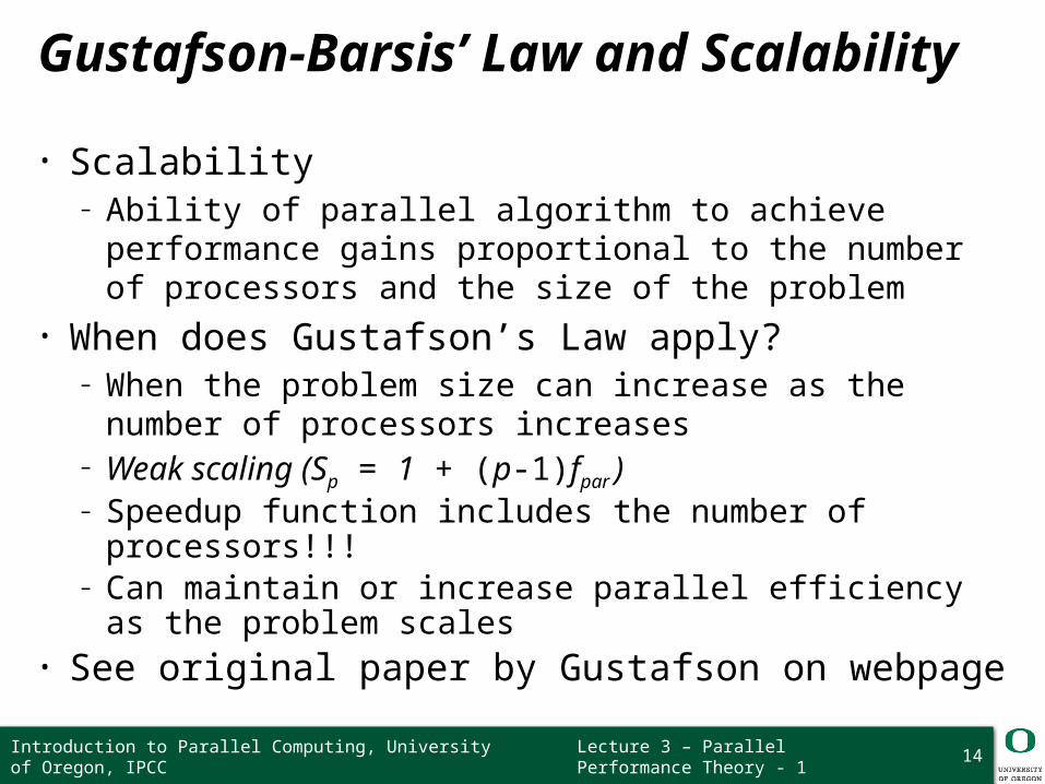
Gustafson-Barsis’ Law and Scalability

• Scalability– Ability of parallel algorithm to achieve performance gains

proportional to the number of processors and the size of the problem

• When does Gustafson’s Law apply?– When the problem size can increase as the number of

processors increases– Weak scaling (Sp = 1 + (p-1)fpar )– Speedup function includes the number of processors!!!– Can maintain or increase parallel efficiency as the problem

scales• See original paper by Gustafson on webpage

14Introduction to Parallel Computing, University of Oregon, IPCC

Lecture 3 – Parallel Performance Theory - 1

Amdahl versus Gustafson-Baris

15Introduction to Parallel Computing, University of Oregon, IPCC

Lecture 3 – Parallel Performance Theory - 1

Amdahl versus Gustafson-Baris

16Introduction to Parallel Computing, University of Oregon, IPCC

Lecture 3 – Parallel Performance Theory - 1

DAG Model of Computation Think of a program as a directed acyclic graph (DAG) of

tasks❍ A task can not execute until all the

inputs to the tasks are available❍ These come from outputs of earlier

executing tasks❍ DAG shows explicitly the task dependencies

Think of the hardware as consistingof workers (processors)

Consider a greedy scheduler ofthe DAG tasks to workers❍ No worker is idle while there

are tasks still to execute17Introduction to Parallel Computing, University of Oregon, IPCC

Lecture 3 – Parallel Performance Theory - 1

Work-Span Model

TP = time to run with P workers

T1 = work❍ Time for serial execution

◆execution of all tasks by 1 worker

❍ Sum of all work T∞ = span

❍ Time along the critical path Critical path

❍ Sequence of task execution (path) through DAG that takes the longest time to execute

❍ Assumes an infinite # workers available18Introduction to Parallel Computing, University of Oregon, IPCC

Lecture 3 – Parallel Performance Theory - 1

Work-Span Example Let each task take 1 unit of time DAG at the right has 7 tasks T1 = 7

❍ All tasks have to be executed❍ Tasks are executed in a serial order❍ Can the execute in any order?

T∞ = 5❍ Time along the critical path❍ In this case, it is the longest pathlength of

any task order that maintains necessary dependencies

19Introduction to Parallel Computing, University of Oregon, IPCC

Lecture 3 – Parallel Performance Theory - 1

Lower/Upper Bound on Greedy Scheduling Suppose we only have P workers We can write a work-span formula

to derive a lower bound on TP

❍ Max(T1 / P , T∞ ) ≤ TP

T∞ is the best possible execution time Brent’s Lemma derives an upper bound

❍ Capture the additional cost executingthe other tasks not on the critical path

❍ Assume can do so without overhead❍ TP ≤ (T1 - T∞ ) / P + T∞

20Introduction to Parallel Computing, University of Oregon, IPCC

Lecture 3 – Parallel Performance Theory - 1

Consider Brent’s Lemma for 2 Processors

T1 = 7

T∞ = 5

T2 ≤ (T1 - T∞ ) / P + T∞

≤ (7 – 5) / 2 + 5

≤ 6

21Introduction to Parallel Computing, University of Oregon, IPCC

Lecture 3 – Parallel Performance Theory - 1

Amdahl was an optimist!

22Introduction to Parallel Computing, University of Oregon, IPCC

Lecture 3 – Parallel Performance Theory - 1

Estimating Running Time

Scalability requires that T∞ be dominated by T1

TP ≈ T1 / P + T∞ if T∞ << T1

Increasing work hurts parallel execution proportionately

The span impacts scalability, even for finite P

23Introduction to Parallel Computing, University of Oregon, IPCC

Lecture 3 – Parallel Performance Theory - 1

Parallel Slack Sufficient parallelism implies linear speedup

24Introduction to Parallel Computing, University of Oregon, IPCC

Lecture 3 – Parallel Performance Theory - 1

Asymptotic Complexity Time complexity of an algorithm summarizes how

the execution time grows with input size Space complexity summarizes how memory

requirements grow with input size Standard work-span model considers only

computation, not communication or memory Asymptotic complexity is a strong indicator of

performance on large-enough problem sizes and reveals an algorithm’s fundamental limits

25Introduction to Parallel Computing, University of Oregon, IPCC

Lecture 3 – Parallel Performance Theory - 1

Definitions for Asymptotic Notation Let T(N) mean the execution time of an algorithm Big O notation

❍ T(N) is a member of O(f(N)) means thatT(N) ≤ cf(N) for constant c

Big Omega notation❍ T(N) is a member of Ω(f(N)) means that

T(N) ≥ cf(N) for constant c Big Theta notation

❍ T(N) is a member of Θ(f(N)) means thatc1f(n) ≤T(N) < c2f(N) for constants c1 and c2

26Introduction to Parallel Computing, University of Oregon, IPCC